Approximation-Robust Inference in Dynamic Discrete Choice

Abstract

Estimation and inference in dynamic discrete choice models often relies on approximation to lower the computational burden of dynamic programming. Unfortunately, the use of approximation can impart substantial bias in estimation and results in invalid confidence sets. We present a method for set estimation and inference that explicitly accounts for the use of approximation and is thus valid regardless of the approximation error. We show how one can account for the error from approximation at low computational cost. Our methodology allows researchers to assess the estimation error due to the use of approximation and thus more effectively manage the trade-off between bias and computational expedience. We provide simulation evidence to demonstrate the practicality of our approach.

Models of dynamic decision making have been applied to a wide range of important problems in empirical economics (see Keane et al., (2011) for a survey). In these models agents face a dynamic decision problem that can often be solved only numerically and at substantial computational cost. Estimation of these models generally requires that the empirical practitioner solve the agents’ dynamic programming problem for each candidate set of parameter values as the likelihood is maximized or GMM objective minimized. For estimation to be computationally feasible, the researcher may need to use approximate dynamic programming methods. The most common approach in empirical economics is approximation of the ‘value function’ or of related functions like the expected value function or the choice-specific expected value function. The function is iteratively interpolated between a small subset of states using say, polynomials, splines, or kernel regression.

Approximation of the solution to the dynamic programming problem has a long history both in operations research and in econometrics. Bellman et al., (1963) suggests a method based on polynomial approximation of the expected value function. Approximate dynamic programming methods were introduced to empirical economics by Keane & Wolpin, (1992) who developed an interpolation method designed for use in finite-horizon dynamic discrete choice models. More recent work includes that of Norets, (2012) who approximates the expected value function using artificial neural networks in the dynamic discrete choice setting.

In many cases value function approximation occurs implicitly. When the state space is continuous some kind of interpolation of the value function is unavoidable, and in many cases models with a discrete state-space implicitly approximate a true model with a continuous state-space.

Unfortunately, the use of approximation leads to inconsistent estimates, and confidence intervals that do not account for the approximation error are not asymptotically valid. One employs approximation methods hoping that the resulting bias is not of too great a magnitude. Without explicit bounds on the approximation error it is unclear how close the approximated value function is to the true value function and it is also unclear how sensitive the estimates are to the approximation error.

Monte Carlo simulation can be used to assess the biases due to approximation (see Keane & Wolpin, (1992)) but simulation studies are inherently limited. Firstly, the findings of simulation studies apply only to the specific model that is simulated. Secondly, one must be able to exactly solve the dynamic programming problem in order to simulate the data, which means that simulation studies can only be carried out on relatively simple models without a very large state space.

Ideally estimation and inference would explicitly account for the use of approximation. We show how this can be achieved. Using the contraction mapping property of the Bellman operator as well as some other features of the problem, we derive bounds on the differences between choices of the choice-specific expected value function. These bounds can be calculated at relatively little computational cost. Using these bounds one can attain a set estimate that must contain the infeasible estimate that could be evaluated if the researcher were able to fully solve the dynamic programming problem. The bounds can be used to achieve confidence sets that are valid regardless of the closeness of the approximation.

Bounds on the approximation error in approximate dynamic programming are considered in for example Arcidiacono et al., (2013), but these bounds are generally on the value function, expected value function, or choice-specific expected value function itself. The value function enters the likelihood only through the differences between the the expected values at different choices. We directly bound the latter and then, using these bounds, derive error bounds on the likelihood.

We develop set estimates and confidence sets that are asymptotically valid regardless of the distance between the exact value function. Our methodology is valid regardless of the method used to approximate the value function.

In short, we provide a methodology that allows researchers to conduct asymptotically valid inference and consistent set estimation, regardless of the accuracy of their value function approximation. Of course, if the approximation is poor then the resulting set estimates and confidence sets will be large, but if the approximation is close they will be small.

Our methodology allows a researcher to directly assess the closeness of their approximation, and balance the trade-off between ease of computation and accuracy of estimation. If the researcher observes that the set estimates and robust confidence intervals are very large compared to standard non-robust confidence sets, then they can decrease the coarseness of their discretization of the state space, increase the order of the approximating polynomial, etc. The tools presented in this paper also apply to novel methods of approximate dynamic programming like Q-learning. Economic researchers might be reluctant to try less well-established methods because they fear that the strength of the approximation may be poor. Our methodology can allay these fears because it allows researchers to explicitly assess the biases due to approximation error and perform estimation and inference that is robust to this type of error.

The paper is organized as follows: Section 1 describes the general model in which the results apply and provides background to the problem. Section 2 provides the derivation of bounds on the value function differences. Section 3 explains how the bounds can be used for estimation and inference that is robust to approximation. Section 4 provides Monte Carlo evidence of the efficacy of the method, and Section 5 concludes.

1 Background

Modeling Dynamic Discrete Choices

Consider an agent who at a each time $t$ is at some state $S_{t}\in\mathcal{S}$ and makes choice $D_{t}\in\mathcal{D}$. The ‘choice set’ $\mathcal{D}$ is assumed to be discrete, but we make no such assumption about the ‘state space’ $\mathcal{S}$. The state evolves according to a first-order Markov process in which the probability distribution of next period’s state may depend on both the current state $S_{t}$ and choice $D_{t}$, and is otherwise unrelated to the history of states and choices. The static utility of the agent in each period is given by $u(S_{t},D_{t})+\epsilon_{t}(D_{t})$ where $\epsilon_{t}$ is an additive iid random function from $\mathcal{D}$ to $\mathbb{R}$. We refer to $\epsilon_{t}$ as ‘shocks’ to the utility because they are not known to the agent prior to period $t$. We assume throughout that $E[\max_{d\in\mathcal{D}}\epsilon_{t}(d)]<\infty$. We assume the deterministic part of the utility $u$ is bounded, i.e., there exists a scalar $b<\infty$ so that $|u(s,d)|\leq b$ for all $s\in\mathcal{S}$ and $d\in\mathcal{D}$.

The agent sets $D_{t}=d(S_{t},\epsilon_{t})$, where $d(\cdot,\cdot)$ is a static decision rule that maximizes the expected discounted (by discount factor $\beta$) sum of utilities:

$$d\in\underset{d:S\times E\to D}{\arg\sup}E\bigg{[}\sum_{t=1}^{\infty}\beta^{t}u\big{(}S_{t},d(S_{t},\epsilon_{t})\big{)}+\epsilon_{t}\big{(}d(S_{t},\epsilon_{t})\big{)}\bigg{]}$$

There are potentially two sources of uncertainty in the agent’s problem. Firstly, $\epsilon_{t}$ is a random function. Secondly, the transition between states may be stochastic. We denote by $F_{s,d}$ the probability distribution of the random variable $S_{t+1}$ for an agent who at time $t$ is at state $S_{t}=s$ and chooses $D_{t}=d$. $F_{s,d}$ is referred to as the ‘transition distribution’ at $(s,d)$ and we refer to $F$, which maps from $(s,d)$ to $F_{s,d}$ as the ‘transition rule’. That the state in the next period depends on the decision in the current period is what makes the agent’s problem ‘dynamic’: the decision today effects not only today’s utility, but the utility tomorrow because it partially determines tomorrow’s state.

If the dynamic optimization problem is sufficiently regular, then the decision rule $d(s,\epsilon)$ is the unique solution to the following static optimization problem:

$$d(s,\epsilon)=\underset{d\in\mathcal{D}}{\arg\max}[u(s,d)+\epsilon(d)+\beta V(s,d)]$$

Where $V:\mathcal{S}\times\mathcal{D}\to\mathbb{R}$ is the unique fixed point of the non-linear operator $T:\mathbb{R}^{(\mathcal{S}\times\mathcal{D})}\to\mathbb{R}^{(\mathcal{S}\times\mathcal{D})}$ which is defined below:

$$T[V](s,d)=E\big{[}E[\max_{d^{\prime}}\,u(S_{t+1},d)+\beta V(S_{t+1},d)+\epsilon_{t+1}(d)|S_{t+1}]\big{|}S_{t}=s,D_{t}=d\big{]}$$ (1)

And so $V$ solves the non-linear operator equation:

$$V=T[V]$$ (2)

This characterization of the optimal decision rule is due to the work of Bellman (see Bellman, (1957)), and is therefore known as ‘Bellman’s principle of optimality’. We refer to $V$ as the ‘choice-specific expected value function’ or just as the ‘value function’ for short. Note that in the literature the ‘value function’ usually refers to instead to the quantity $\max_{d}u(s,d)+\epsilon(d)+\beta V(s,d)$ which is a function of both $s$ and $\epsilon$. $\beta V(s,d)$ is the expected discounted future returns from time $t+1$ onwards for an agent who, at time $t$, is at state $s$ and makes choice $d$, and acts optimally thereafter. We refer to (2) as the ‘Bellman equation’ and $T$ as the ‘Bellman operator’ although these terms are often used slightly differently (see Keane et al., (2011)).

Point Estimation

To create a statistical model within the dynamic discrete choice framework let us introduce a vector of parameters of interest $\theta$. $\theta$ may parameterize the utility function, the distribution of $\epsilon_{t}$, and the state transition rule $F$. For simplicity we focus on the case in which $\theta$ parameterizes the utility and distribution of $\epsilon_{t}$. Both the utility function and distribution of $\epsilon_{t}$ are treated as known up to the parameters $\theta$. To emphasize the dependence of the utility function on $\theta$ we let $u(s,d;\theta)$ be the deterministic part of the utility at state $s$ and from choice $d$ under the parameters $\theta$.

Note that the Bellman operator (1) depends on the utility function, thus the solution $V$ to the Bellman equation (2) depends on the parameters $\theta$ and discount factor $\beta$. In addition, the Bellman operator depends on the transition rule $F$ and therefore so does the solution $V$. To make clear this dependence we write $V_{(\theta,\beta,F)}(s,d)$ to denote the choice-specific expected value function at choice $d$ and state $s$ when the utility parameters are equal to $\theta$, the discount factor equals $\beta$, and the transition rule is $F$.

It will be convenient to define the differences in shocks, utilities and choice-specific values between pairs of choices $d$ and $d^{\prime}$:

$$\Delta_{d,d^{\prime}}\epsilon_{t} =\epsilon_{t}(d)-\epsilon_{t}(d^{\prime})$$

$$\Delta_{d,d^{\prime}}u(s;\theta) =u(s,d;\theta)-u(s,d^{\prime};\theta)$$

$$\Delta V_{(\theta,\beta,F)}(s,d,d^{\prime}) =V_{(\theta,\beta,F)}(s,d)-V_{(\theta,\beta,F)}(s,d^{\prime})$$

Given the model in the previous section, the probability that an agent at state $S_{t}=s$ makes decision $D_{t}=d$ is given by:

$$L_{(\theta,\beta;F)}(s,d)=P_{\theta}\bigg{[}\Delta_{d,d^{\prime}}\epsilon_{t}\geq\Delta_{d^{\prime},d}u(s;\theta)+\beta\Delta V_{(\theta,\beta,F)}(s,d^{\prime},d),\forall d^{\prime}\in\mathcal{D}\bigg{]}$$ (3)

Where $P_{\theta}$ is the probability given the distribution of $\epsilon_{t}$ which possibly depends on parameters $\theta$. If the transition rule $F$ were known then $L_{(\theta,\beta;F)}(S_{t},D_{t})$ is the likelihood of the observation $(S_{t},D_{t})$ at time $t$. If $F$ is unknown then it is a nuisance parameter. $F$ can be estimated directly from the data in a first stage either parametrically or nonparametrically. Let $\hat{F}$ be some estimate of $F$ that is evaluated in a first stage. With $F$ replaced by the estimate $\hat{F}$, the partial log-likelihood of the data $\{S_{t},D_{t}\}_{t=1}^{T}$ evaluated at parameters $\theta$ and $\beta$ is then given by:

$$\mathcal{L}_{\{S_{t},D_{t}\}_{t=1}^{T}}(\theta,\beta;\hat{F})=\sum_{t=1}^{T}\ln L_{(\theta,\beta;\hat{F})}(S_{t},D_{t})$$

An estimate of the parameters $\theta$ and $\beta$ is then given by:

$$(\hat{\theta},\hat{\beta})=\arg\max_{\theta,\beta}\mathcal{L}_{\{S_{t},D_{t}\}_{t=1}^{\infty}}(\theta;\beta,\hat{F})$$

Identification of the discount factor can be difficult (see Rust, (1987), Magnac & Thesmar, (2002), Abbring & ystein Daljord, (2020)), and so the discount factor may be calibrated in some applications. In this case one can simply plug-in the assumed value for $\beta$ and maximize the log-likelihood only over the argument $\theta$. The maximization problem above seldom admits a closed-form solution, and so numerical optimization methods are required. Thus, for a number of candidate values of $\theta$ and possibly $\beta$ one must evaluate $\mathcal{L}_{\{S_{t},D_{t}\}_{t=1}^{T}}(\theta,\beta;\hat{F})$ and/or its derivatives. In order to calculate $\mathcal{L}_{\{S_{t},D_{t}\}_{t=1}^{T}}(\theta,\beta;F)$ one must evaluate the value function differences $\Delta V_{(\theta,\beta,F)}(s,d^{\prime},d)$ at all choices in $\mathcal{D}$ and at all states observed in the data. This procedure is known as the ‘nested fixed point’ or NFXP algorithm because nested within each step of a numerical maximum likelihood procedure one applies an algorithm to find a fixed point of the Bellman operator (Wolpin, (1984), Rust, (1987)).

The standard method for evaluating $V$ at all realized states up to close approximation is ‘Bellman iteration’. To apply the method one begins with some guess of the solution $V_{(\theta,\beta,F)}(\cdot,\cdot)$ and then iteratively applies the Bellman operator until there is little change between iterations. Let us be more precise. Let $T_{(\theta,\beta,F)}$ be the Bellman operator (defined in (1)) when the parameters are set to values $\theta$, $\beta$ and $F$. For any $n\in\mathbb{N}$ and $\tilde{V}$, let $T_{(\theta,\beta,F)}^{n}[\tilde{V}]=\big{[}T_{(\theta,\beta,F)}^{n-1}[\tilde{V}]\big{]}$ and let $T_{(\theta,\beta,F)}^{1}[\tilde{V}]=T_{(\theta,\beta,F)}[\tilde{V}]$. Then for some initial guess $\tilde{V}_{0}$ one approximates $V_{(\theta,\beta,F)}(\cdot,\cdot)$ by $T_{(\theta,\beta,F)}^{n}[\tilde{V}_{0}](s,d)$ where $n$ is large enough that $T_{(\theta,\beta,F)}^{n}[\tilde{V}_{0}]$ and $T_{(\theta,\beta,F)}^{n-1}[\tilde{V}_{0}]$ sufficiently close in some sense. Because $T_{(\theta,\beta,F)}$ is a contraction mapping, one can show that for any bounded function $\tilde{V}_{0}$, $T_{(\theta,\beta,F)}^{n}[\tilde{V}_{0}]$ converges in the supremum norm to the unique fixed point of $T_{(\theta,\beta,F)}$ as $n\to\infty$.

Unfortunately, each iteration of the fixed point procedure above requires that one evaluate the right hand side of (1) at every state $s$ and choice $d$, not just those states and decisions observed in the data. If the state space is discrete but large then this can be computationally burdensome and if the state space is not discrete and finite it is generally impossible. This same problem applies for many alternative methods of finding a fixed point to the Bellman equation like Newton-Kantorovich.

An alternative to the NXFP algorithm, Mathematical Program with Equilibrium Constraints (MPEC) avoids the need for Bellman iteration (Su & Judd, (2012)). MPEC treats the estimation problem as a constrained optimization problem in which both $\theta$ and (possibly) $\beta$ and the value function itself are parameters and the the Bellman equation (2) is treated as a constraint. Thus in MPEC the number of scalar constraints is proportional to the cardinality of the state space. As such, when the state space is large MPEC may still be computationally burdensome.

In many cases, the RHS of (1) cannot be evaluated exactly even at a single state and choice. The expectation over the future states on the RHS of (1) generally does not have an analytical form and so must be evaluated by numerical methods. The inner expectation on the RHS of (1) may also be analytically intractable. For instance, this is the case when $\epsilon_{t}$ (understood as a vector with each entry corresponding to $\epsilon_{t}(d)$ for some $d\in\mathcal{D}$) is multivariate normal with a non-diagonal covariance matrix. This further compounds the computational burden of applying the Bellman operator at a large number of states.

To avoid the need to evaluate the RHS of the Bellman equation at a large and possibly infinite number of states, some kind of approximation is needed. For example, one may apply the Bellman operator at only some subset of states and then for other states approximate the value function as needed by interpolation. Let us denote by $\tilde{T}_{(\theta,\beta,F)}$ an approximate Bellman operator so that $\tilde{T}_{(\theta,\beta,F)}[\tilde{V}](s,d)=T_{(\theta,\beta,F)}[\tilde{V}](s,d)$ for all $s$ in some small, finite subset $\tilde{\mathcal{S}}\subset\mathcal{S}$ and all choices $d\in\mathcal{D}$ and for all other $s\in\mathcal{S}$ and $d\in\mathcal{D}$ takes some value given by interpolation. We refer to $\tilde{\mathcal{S}}$ as a ‘discrete grid’. It is important to note that in general, $\tilde{T}$ is not a contraction. The term ‘interpolation’ is used here as a catch-all for a range of different approaches that include fitting a parametric function by least squares, kernel methods and modern machine-learning regression techniques like random forests.

If one replaces $\Delta_{(\theta,\beta,F)}V(s;d^{\prime},d)$ in the expression for the likelihood (3) with an approximation, then one evaluates the log-likelihood with error. Thus the resulting maximum likelihood estimates will generally be inconsistent. When applying approximation methods one hopes that the approximated value function differences are close to the exact differences $\Delta_{(\theta,\beta,F)}V(s,d^{\prime},d)$, that the approximate log-likelihood is then close to the exact log-likelihood, and that the estimates are then close to the exact maximum likelihood estimates and the degree of inconsistency is therefore small. The need to bound the estimation error that results from value function approximation motivates the method described in the next section.

Finally, we note that a class of methods referred to as Conditional Choice Probability (CCP) methods side-step the need for dynamic programming entirely. This approach was introduced by Hotz & Miller, (1993), and the literature contains a number of different methods based on their approach, for example Aguirregabiria & Mira, (2007) and Bajari et al., (2007). These methods are based on the observation that under the structure of a given dynamic discrete choice model, the value function is often equal to an analytic (or easy to numerically compute) function of the choice probabilities of the agent at each state. Thus in a first stage one nonparametrically estimates from the data the probability of each discrete choice at each stage and plugs this in to get an estimate of the value function. However, these methods have certain drawbacks. The first-stage nonparametric choice probability estimation contributes to the variance and bias of the parameter estimates, and so the parameter estimates are generally inefficient compared to estimates based on dynamic programming. This is particularly problematic because the choice probabilities may be very imprecisely estimates at parts of the state space that are visited with very low probability (for further discussion see Aguirregabiria & Mira, (2007)).

Our method can be used regardless of the manner in which the value function is approximated or estimated and can therefore complement CCP methods. Firstly, our method allows for valid inference and consistent set estimation even when the conditional choice probabilities cannot be consistently estimated. Secondly, our inference method does not need to account for any first stage nonparametric estimation of the conditional choice probabilities and as such confidence sets based on our method could be smaller than those based on CCP point estimates.

2 Bounding the Approximation Error

In the previous section we discussed the need for approximation methods in the evaluation of the value function differences $\Delta_{(\theta,\beta,F)}V$ at the states observed in the data. In this section we describe how one can bound the difference between the exact value function differences $\Delta_{(\theta,\beta,F)}V$ and the differences from some approximate value function $\tilde{V}$. In Section 3 we show how these bounds can be used to achieve set estimation and inference that is valid regardless of the approximation error.

For ease of notation let us again suppress the arguments $\theta$, $\beta$, and $F$ in the value function $V$ and Bellman operator $T$. Theorem 1 below provides an upper bound on the distance between the exact value function differences $V(s,d)-V(s,d^{\prime})$ and the differences $\tilde{V}(s,d)-\tilde{V}(s,d^{\prime})$ for some approximate value function $\tilde{V}$. The theorem refers to a function $b(s,d,d^{\prime})$ defined as follows:

$$b(s,d,d^{\prime})=\frac{1-\beta[\sup_{s,s^{\prime}\in S,d,d^{\prime}\in D}\delta(F_{s,d},F_{s^{\prime},d^{\prime}})]+\beta\delta(F_{s,d},F_{s,d^{\prime}})}{1-\beta[\sup_{s,s^{\prime}\in S,d,d^{\prime}\in D}\delta(F_{s,d},F_{s^{\prime},d^{\prime}})]}$$

Where $\delta(F_{s,d},F_{s^{\prime},d^{\prime}})$ is the total variation distance between $F_{s,d}$ and $F_{s^{\prime},d^{\prime}}$.

Theorem 1.

Suppose $u$ is bounded and $E[\max_{d\in\mathcal{D}}\epsilon_{t}(d)]<\infty$. Let $V$ solve the Bellman equation (2) for transition rule $F$ and discount factor $\beta<1$. For any $d,d^{\prime}\in\mathcal{D}$ and $s\in\mathcal{S}$ and bounded function $\tilde{V}$ on $(\mathcal{S}\times\mathcal{D})$:

$$\big{|}\big{(}\tilde{V}(s,d)-\tilde{V}(s,d^{\prime})\big{)}-\Delta V(s,d,d^{\prime})\big{|}$$

$$\leq b(s,d,d^{\prime})\sup_{s,s^{\prime}\in S,d,d^{\prime}\in D}|[T[\tilde{V}](s^{\prime},d^{\prime})-T[\tilde{V}](s,d)]-[\tilde{V}(s^{\prime},d^{\prime})-\tilde{V}(s,d)]]|$$

The upper bound given in Theorem 1 does not involve the exact value function $V$. Instead it involves only the discount factor $\beta$, the transition law $F$, and the approximate value function $\tilde{V}$. The upper bound is small when the discount factor $\beta$ is small, when the transition distribution $F_{s,d}$ does not change much between states and choices, and when $\tilde{V}$ comes close to satisfying the Bellman equation. Note that in the case where the approximation is exact, i.e. $\tilde{V}=V$ the upper bound is equal to zero.

The total variation distance $\delta(F_{s,d},F_{s^{\prime},d^{\prime}})$, could be computed analytically or numerically depending on the transition law $F$ or first-stage estimate thereof. Note that the total variation distance must be bounded above by $1$ and so:

$$b(s,d,d^{\prime}) \leq\frac{1}{1-\beta}$$

The inequality above allows us to avoid calculating the total variation distance but results in a looser bound than that given in Theorem 1. In order to evaluate the upper-bound in Theorem 1 one must also evaluate the supremum over states $s$ and $s^{\prime}$ and choices $d$ and $d^{\prime}$ of the following quantity:

$$|T\tilde{V}(s,d)-T\tilde{V}(s^{\prime},d^{\prime})-[\tilde{V}(s,d)-\tilde{V}(s^{\prime},d^{\prime})]|$$

It may be feasible to directly evaluate the supremum of the above, however if $\mathcal{S}$ is large then evaluating the supremum is still computationally expensive. If $\mathcal{S}$ is continuous one could discretize the state space before finding the supremum, this of course will still result in approximation error, but this error may be acceptable because it is not compounded by repeated Bellman iteration. For the case where the supremum cannot be effectively computed we describe an algorithm that upper bounds the supremum and that can be run until the exact supremum and upper bound are arbitrarily close.

Define $\bar{b}_{\tilde{V}}$ by:

$$\bar{b}_{\tilde{V}}=\sup_{s,s^{\prime}\in S,d\in D}|u(s,d)+\beta\tilde{V}(s,d)-u(s^{\prime},d)-\beta\tilde{V}(s^{\prime},d)|$$

Note that $\bar{b}_{\tilde{V}}$ can be evaluated without applying the Bellman operator. Further, because $\bar{b}_{\tilde{V}}$ only involves $u$ and $\tilde{V}$ which are generally parametric functions, it may be possible to evaluate (or at least upper bound) $\bar{b}_{\tilde{V}}$ analytically.

Theorem 2 below motivates our algorithm.

Theorem 2.

Let $\mathcal{A}$ be a finite subset of $\mathcal{S}\times\mathcal{D}$, then:

$$\big{|}\big{(}\tilde{V}(s,d)-\tilde{V}(s,d^{\prime})\big{)}-\Delta V(s,d,d^{\prime})\big{|}$$

$$\leq b(s,d,d^{\prime})\sup_{s,s^{\prime}\in S,d,d^{\prime}\in D}\bigg{[}\min_{(s^{*},d^{*})\in\mathcal{A}}\{T[\tilde{V}](s^{*},d^{*})+\delta(F_{s,d},F_{s^{*},d^{*}})\bar{b}_{\tilde{V}}\}$$

$$-\max_{(s^{*},d^{*})\in\mathcal{A}}\{T[\tilde{V}](s^{*},d^{*})-\delta(F_{s^{\prime},d^{\prime}},F_{s^{*},d^{*}})\bar{b}_{\tilde{V}}\}-[\tilde{V}(s,d)-\tilde{V}(s^{\prime},d^{\prime})]\bigg{]}$$

The upper bound in Theorem 2 only requires that one apply the Bellman operator $T$ at those states and choices in the finite set $\mathcal{A}$. The supremum in the upper bound may have an analytical solution for some parametric choices of $\tilde{V}$.

If $\mathcal{A}$ is ‘dense’ in a certain sense, and the functions involved are uniformly continuous, then the bound in Theorem 2 is not very conservative compared to the bound in Theorem 1. We formalize this in Theorem 3 below. Theorem 2 suggests the following procedure to upper bound $\sup_{s,s^{\prime},d,d^{\prime}}|T[\tilde{V}](s,d)-T[\tilde{V}](s^{\prime},d^{\prime})-[\tilde{V}(s,d)-\tilde{V}(s^{\prime},d^{\prime})]|$. The algorithm returns a quantity $\bar{B}$ that is guaranteed (by Theorem 2) to upper bound $\sup_{s,s^{\prime},d,d^{\prime}}|T[\tilde{V}](s,d)-T[\tilde{V}](s^{\prime},d^{\prime})-[\tilde{V}(s,d)-\tilde{V}(s^{\prime},d^{\prime})]|$ and that is guaranteed to exceed this quantity by less than a desired tolerance $\tau$.

1. Choose some finite set of states and choices $\mathcal{A}\subset\mathcal{S}\times\mathcal{D}$. Evaluate $T[\tilde{V}](s,d)$ for each $(s,d)\in\mathcal{A}$. Evaluate $\bar{b}_{\tilde{V}}$.

2. Calculate $\bar{B}$ given by:

   $$\bar{B}= \sup_{s,s^{\prime}\in S,d,d^{\prime}\in D}\bigg{[}\min_{(s^{*},d^{*})\in\mathcal{A}}\{T[\tilde{V}](s^{*},d^{*})+\delta(F_{s,d},F_{s^{*},d^{*}})\bar{b}_{\tilde{V}}\}$$

   $$-\max_{(s^{*},d^{*})\in\mathcal{A}}\{T[\tilde{V}](s^{*},d^{*})-\delta(F_{s^{\prime},d^{\prime}},F_{s^{*},d^{*}})\bar{b}_{\tilde{V}}\}-[\tilde{V}(s,d)-\tilde{V}(s^{\prime},d^{\prime})]\bigg{]}$$

   Evaluate $\underline{B}$ by:

   $$\underline{B}=\max_{(s,d),(s^{\prime},d^{\prime})\in\mathcal{A}}\{|T[\tilde{V}](s,d)-T[\tilde{V}](s^{\prime},d^{\prime})-[\tilde{V}(s,d)-\tilde{V}(s^{\prime},d^{\prime})]|\}$$

3. If $\bar{B}-\underline{B}\leq\tau$ then we are done and $\bar{B}$ is the upper bound. If $\bar{B}-\underline{B}>\tau$ then increase the density of $\mathcal{A}$ and return to step 2 else continue to step 4.

4. Take as the bound $b(s,d,d^{\prime})\bar{B}$.

Note that at each iteration in the algorithm above, the upper bound $\bar{B}$ exceeds $\sup_{s,s^{\prime},d,d^{\prime}}|T[\tilde{V}](s,d)-T[\tilde{V}](s^{\prime},d^{\prime})-[\tilde{V}(s,d)-\tilde{V}(s^{\prime},d^{\prime})]|$. It is not too difficult to see that $\underline{B}$ lower bounds this quantity. Hence $\tau$ bounds the conservativeness of the upper bound $\bar{B}$. In Theorem 3 we provide simple conditions that ensure the algorithm above halts and therefore guarantees we find a bound $\bar{B}$ that is within $\tau$ of the quantity we wish to bound.

We define the density of $\mathcal{A}$ as the reciprocal of $\sup_{s\in\mathcal{S},d\in\mathcal{D}}\min_{(s^{\prime},d)\in\mathcal{A}}||s-s^{\prime}||$ (if the denominator is zero we take the density to be infinity).

Theorem 3.

If $\mathcal{S}\subset\mathbb{R}^{k}$ is compact and the functions $s\mapsto T[\tilde{V}](s,d)$, $s\mapsto\tilde{V}(s,d)$, and $(s,s^{\prime})\mapsto\delta(F_{s,d},F_{s^{\prime},d})$ are each uniformly continuous for all $d\in\mathcal{D}$, then as the density of $\mathcal{A}$ increases to infinity $\bar{B}-\underline{B}\to 0$.

Theorem 3 implies that the algorithm described above must eventually halt and thus ensure that $\bar{B}$ exceeds the bound in Theorem 1 by no more than the pre-specified tolerance $\tau$.

3 Subset Estimation and Robust Inference

Let us reintroduce parameters $\theta$, $\beta$, and $F$ into our notation for the value function $V$ and Bellman operator. For any bounded function $\tilde{V}$, The results in the previous section imply an upper-bound of the form:

$$\big{|}\big{(}\tilde{V}(s,d)-\tilde{V}(s,d^{\prime})\big{)}-\Delta_{(\theta,\beta,F)}V(s,d,d^{\prime})\big{)}\big{|}$$

$$\leq Q_{(\theta,\beta,F)}(s,d,d^{\prime};\tilde{V})$$

Where $Q_{(\theta,\beta,F)}$ is the bound given in Theorem 2 (or possibly Theorem 1 if this can be feasibly calculated) for the particular choice of $\theta$, $\beta$, $F$. Note then that for any $\tilde{V}$:

$$\Delta_{(\theta,\beta,F)}\tilde{V}(s;d^{\prime},d)-Q_{(\theta,\beta,F)}(s,d,d^{\prime};\tilde{V})$$

$$\leq \Delta_{(\theta,\beta,F)}V(s;d^{\prime},d)$$

$$\leq \Delta_{(\theta,\beta,F)}\tilde{V}(s;d^{\prime},d)+Q_{(\theta,\beta,F)}(s,d,d^{\prime};\tilde{V})$$

For any bounded function $\hat{V}:\mathcal{D}\to\mathbb{R}$ let:

$$L_{(\theta,\beta,F)}(s,d;\hat{V})=P_{\theta}\bigg{[}\Delta_{d,d^{\prime}}\epsilon_{t}\geq\Delta_{d^{\prime},d}u(s;\theta)+\beta\hat{V}(d^{\prime}),\forall d^{\prime}\in\mathcal{D},d^{\prime}\neq d\bigg{]}$$

Note that $L_{(\theta,\beta,F)}(s,d)=L_{(\theta,\beta,F)}\big{(}s,d;\Delta V_{(\theta,\beta,F)}(s,d,\cdot)\big{)}$. It is easy to see that $L_{(\theta,\beta,F)}(s,d;\hat{V})$ is monotonically decreasing in $\hat{V}(d^{\prime})$ for each $d^{\prime}\neq d$. As such, for any bounded $\tilde{V}:\mathcal{S}\times\mathcal{D}\to\mathbb{R}$:

$$L_{(\theta,\beta,F)}\big{(}s,d;\tilde{V}(s,\cdot)-\tilde{V}(s,d)+Q_{(\theta,\beta,F)}(s,d,\cdot;\tilde{V})\big{)}$$

$$\leq L_{(\theta,\beta,F)}(s,d)$$

$$\leq L_{(\theta,\beta,F)}\big{(}s,d;\tilde{V}(s,\cdot)-\tilde{V}(s,d)-Q_{(\theta,\beta,F)}(s,d,\cdot;\tilde{V})\big{)}$$

So we have found upper and lower bounds the likelihood. Thus we can define an upper- bound on the sample log likelihood of the data by:

$$\mathcal{L}_{\{S_{t},D_{t}\}_{t=1}^{T}}^{U}(\theta,\beta;F,\tilde{V})$$

$$= \sum_{t=1}^{T}\ln L_{(\theta,\beta,F)}\big{(}S_{t},D_{t};\tilde{V}(s,\cdot)-\tilde{V}(s,d)-Q_{(\theta,\beta,F)}(S_{t},D_{t},\cdot;\tilde{V})\big{)}$$

And a lower bound by:

$$\mathcal{L}_{\{S_{t},D_{t}\}_{t=1}^{T}}^{L}(\theta,\beta;F,\tilde{V})$$

$$= \sum_{t=1}^{T}\ln L_{(\theta,\beta,F)}\big{(}S_{t},D_{t};\tilde{V}(s,\cdot)-\tilde{V}(s,d)+Q_{(\theta,\beta,F)}(S_{t},D_{t},\cdot;\tilde{V})\big{)}$$

Now suppose that $\hat{\theta}^{*}$ and $\hat{\beta}^{*}$ maximize the exact log likelihood $\mathcal{L}_{\{S_{t},D_{t}\}_{t=1}^{T}}(\theta,\beta;\hat{F})$ (the log-likelihood obtained if the full dynamic programming solution were available). Suppose we have some approximate dynamic programming algorithm that, for each $\theta$, $\beta$ and $F$, provides an approximate value function $\tilde{V}_{(\theta,\beta,F)}$. It follows that:

$$\mathcal{L}_{\{S_{t},D_{t}\}_{t=1}^{T}}^{U}(\hat{\theta}^{*},\hat{\beta}^{*};\hat{F},\tilde{V}_{(\hat{\theta}^{*},\hat{\beta}^{*},\hat{F})})\geq\sup_{\theta,\beta}\mathcal{L}_{\{S_{t},D_{t}\}_{t=1}^{T}}^{L}(\theta,\beta;\hat{F},\tilde{V}_{(\theta,\beta,\hat{F})})$$

Note that the inequality above applies regardless of the algorithm used to generate $\tilde{V}_{(\theta,\beta,F)}$. The above implies that $(\hat{\theta}^{*},\hat{\beta}^{*})$ lies in the following set:

$$\bigg{[}(\theta,\beta):\mathcal{L}_{\{S_{t},D_{t}\}_{t=1}^{T}}^{U}(\theta,\beta;\hat{F},\tilde{V}_{(\theta,\beta,\hat{F})})\geq\sup_{\theta^{\prime},\beta^{\prime}}\mathcal{L}_{\{S_{t},D_{t}\}_{t=1}^{T}}^{L}(\theta^{\prime},\beta^{\prime};\hat{F},\tilde{V}_{(\theta^{\prime},\beta^{\prime},\hat{F})})\bigg{]}$$

The set above can be used as a set estimator for the true parameters $\theta$ and $\beta$. By construction the set estimator must contain the infeasible maximum likelihood estimates, that is, the estimates obtained if the full dynamic programming solution were available. If the infeasible maximum likelihood estimates $\hat{\theta}^{*}$ and $\hat{\beta}^{*}$ are consistent estimates, then set estimator is consistent (in the Hausdorff metric).

We can also use the upper and lower bounds on the likelihood to derive confidence sets that are valid regardless of the accuracy of the approximate value function $\tilde{V}_{(\theta,\beta,\hat{F})}$. The standard likelihood-ratio confidence set for the parameters is given by:

$$[(\theta,\beta):\>2\big{(}\sup_{\theta^{\prime},\beta^{\prime}}\mathcal{L}_{\{S_{t},D_{t}\}_{t=1}^{T}}(\theta^{\prime},\beta^{\prime};\hat{F})-\mathcal{L}_{\{S_{t},D_{t}\}_{t=1}^{T}}(\theta,\beta;\hat{F})\big{)}\leq c_{1-\alpha}]$$

where $c_{1-\alpha}$ is the $1-\alpha$-level critical value, usually the $\alpha$-quantile of the chi-squared distribution with degrees of freedom equal to the dimension of $\theta$ and $\beta$. The above is infeasible, it cannot be evaluated because $\mathcal{L}_{\{S_{t},D_{t}\}_{t=1}^{T}}$ incorporates the exact solution to the dynamic programming problem. However the confidence set above is necessarily a subset of the following feasible set:

$$[(\theta,\beta):\>2\big{(}\sup_{\theta^{\prime},\beta^{\prime}}\mathcal{L}_{\{S_{t},D_{t}\}_{t=1}^{T}}^{U}(\theta^{\prime},\beta^{\prime};\hat{F},\tilde{V}_{(\theta,\beta,\hat{F})})-\mathcal{L}_{\{S_{t},D_{t}\}_{t=1}^{T}}^{L}(\theta,\beta;\hat{F},\tilde{V}_{(\theta,\beta,\hat{F})})\big{)}\leq c_{1-\alpha}]$$

Thus, if the exact, infeasible likelihood ratio-based confidence set has asymptotically correct size, then so too must the feasible one based on approximate dynamic programming above.

4 Monte Carlo Exercise

As a practical demonstration of our methods we present a Monte Carlo simulation. We simulate data from a modified Rust model (Rust, (1987)). We apply our methods to account for approximation error in maximum likelihood estimates that employ approximate dynamic programming. We evaluate set estimates and robust confidence sets when the approximate dynamic programming is applied with differing degrees of coarseness. We compare our set estimates and robust confidence sets to conventional point estimates and confidence sets that do not account for the error due to approximation in the value function.

In the modified Rust model, at each period a decision maker chooses whether or not to send a bus engine for repairs. The choice set is binary $\mathcal{D}=\{0,1\}$ with $d=0$ representing the decision not to repair the engine and $d=1$ the decision to repair the engine. The state space is given by $\mathcal{S}=[0,20]$, each $s\in\mathcal{S}$ represents a possible value for the engine’s mileage given in thousands of miles. We treat the mileage as a metaphor for the general health the engine and thus it is possible for the mileage to decrease between periods. The cost of running (and not repairing) an engine increases with the mileage because with high mileage the engine becomes unreliable and fuel-hungry. At state $s$ running the engine incurs a cost of $-\theta_{1}{s}$ where $\theta_{1}$ is a scalar parameter. Repairing an engine incurs a fixed cost of $-\theta_{2}$ regardless of the mileage. Thus the deterministic parts of the utilities from the two choices at state $s$ are given by $u(s,0)=\theta_{1}{s}$ and $u(s,1)=\theta_{2}$.

In each period $t$ there is an additive, stochastic shock to both the cost of repair and non-repair. The cost shock to non-repair and repair in period $t$ are respectively $\epsilon_{t}(0)$ and $\epsilon_{t}(1)$. The shocks are iid and independent between the two choices, they are observed by the decision-maker before making a decision at time $t$ but are not known prior to $t$. We let the shocks be standard type-1 extreme value distributed. The bus’s route is subject to unexpected changes due to road closures and driver error, as such the mileage evolves stochastically. If the decision at time $t$ is $D_{t}$ and the engine has mileage $S_{t}$, then the mileage in period $t+1$ is distributed according to:

$$S_{t+1}|S_{t},D_{t}\sim\min\{\max\{0,S_{t}+1\{D_{t}=0\}\gamma_{1}+1\{D_{t}=1\}\gamma_{2}+U[-\gamma_{3},\gamma_{3}]\},50\}$$

Where $U[-\gamma_{3},\gamma_{3}]$ is a uniform random variable between $-\gamma_{3}$ and $\gamma_{3}$. $\gamma_{1}$, $\gamma_{2}$, and $\gamma_{3}$ are model parameters. In our simulations $\gamma_{2}$ is negative, thus repair of the engine reduces the mileage.

The modified replacement model differs from Rust’s original formulation in two key ways. Firstly, we treat the mileage as a continuous variable, In the original model estimated by Rust the mileage is discretized. Secondly, in the modified model the decision maker chooses whether or not to repair the engine, reducing its effective mileage by some fixed amount. In the original model the decision maker chooses whether or not to replace the engine, bringing the mileage down to zero. The use of a continuous state-space allows us to examine our method when the value function is approximated with different degrees of coarseness. Repairing rather than replacing the engine ensures that the total variation distance $\delta(F_{s,0},F_{s,1})$ is strictly less than unity even for large values of $s$. Without this feature the factor $b(s,d,d^{\prime})$ in the upper bound in Theorem 1 would be equal to $\frac{1}{1-\beta}$ when the mileage $s$ is large. Thus this modeling decision allows us to demonstrate the improvement our specific bound provides over the more crude bound with a factor of $\frac{1}{1-\beta}$ when the distribution of future states from different choices overlaps.

Note that in the model above:

$$b(s,d,d^{\prime})\leq\frac{1-\beta+\beta\min\{|\frac{\gamma_{1}-\gamma_{2}}{2\gamma_{3}}|,1\}}{1-\beta}$$

Note also that because $\epsilon_{t}(d)$ is independently type-1 extreme value distributed for each $d\in\mathcal{D}$ we have for any $\tilde{V}$:

$$T[\tilde{V}](s,d)=E\big{[}ln\big{(}\sum_{d\in\mathcal{D}}\exp(u(S_{t+1},d)+\beta\tilde{V}(S_{t+1},d)\big{)}\big{|}S_{t}=s,D_{t}=d\big{]}+c$$

Where $c$ is the Euler–Mascheroni constant. In order to generate data from the model we must solve for the value function. An exact solution is infeasible and so we apply approximate value function iteration. We employ a dense grid $\tilde{\mathcal{S}}$ that consists of $1001$ evenly spaced points between $0$ and $20$. We replace the outer expectation in the RHS above by an empirical expectation (over $100$ draws of $S_{t+1}$):

$$T[\tilde{V}](s,d)\approx\frac{1}{n}\sum_{i=1}^{n}ln\big{(}\sum_{d\in\mathcal{D}}\exp(u(S_{s,d,i},d)+\beta\tilde{V}(S_{s,d,i},d)\big{)}+c$$

Where $S_{s,d,i}$ is the $i^{th}$ draw from the distribution of $S_{t+1}$ given $S_{t}=s$ and $D_{t}=d$. We begin with an initial guess $V_{0}$ of the value function (our initial guess is that the function equals zero everywhere), and at the $j^{th}$ iteration we evaluate $T[V_{j}](s,d)$ for each $s$ in the dense grid $\tilde{\mathcal{S}}$ and each $d\in\mathcal{D}$. We then linearly interpolate the resulting function between the points in $\tilde{\mathcal{S}}$ in order to evaluate $V_{j+1}(S_{s,d,i},d)$ for each $d\in\mathcal{D}$, $s\in\tilde{\mathcal{S}}$ and $i\in\{1,...,n\}$. Note that the samples $\{\{\{S_{s,d,i}\}_{i=1}^{n}\}_{d\in\mathcal{D}}\}_{s\in\tilde{\mathcal{S}}}$ are drawn before the first iteration and do not change between iterations. We continue until the change in the value function between iterations is smaller than a pre-specified tolerance at all $s\in\tilde{\mathcal{S}}$ and $d\in\mathcal{D}$.

Each simulated dataset consists of $5000$ periods of data generated from the model above. Table 1 summarizes the data generating process and states the parameter values used in the simulation.

Table 1: DGP summary and Parameter Values

Model Parameters	DGP Summary
$\beta=$$0.8$	$\big{(}\epsilon_{t}(0),\epsilon_{t}(1)\big{)}\sim\text{independent type-1 extreme value}$
$\theta_{1}=-0.6$	$u(s,0)=\theta_{1}s$
$\theta_{2}=-4$	$u(s,1)=\theta_{2}$
$\gamma_{1}=1$	$\mathcal{S}=[0,20]$, $\mathcal{D}=\{0,1\}$
$\gamma_{2}=-1$	$S_{t+1}|S_{t},D_{t}=0\sim\min\{\max\{S_{t}+\gamma_{1}+U[-\gamma_{3},\gamma_{3}],20\},0\}$
$\gamma_{3}=5$	$S_{t+1}|S_{t},D_{t}=1\sim\min\{\max\{S_{t}+\gamma_{2}+U[-\gamma_{3},\gamma_{3}],20\},0\}$
$T=1000$	$\tilde{\mathcal{S}}=\{0,\frac{1}{50},\frac{2}{50},...,\frac{999}{50},20\}$

On each simulated dataset we apply maximum likelihood to estimate the parameters $\theta_{1}$ and $\theta_{2}$. We treat $\beta$, $\gamma_{1}$, $\gamma_{2}$, and $\gamma_{3}$ as known. For each candidate set of parameter values in the maximization routine we approximately solve the dynamic programming problem using Bellman iteration on a grid $\hat{\mathcal{S}}$ of evenly spaced points in the interval $[0,20]$ and interpolating as described in Section 1. The interpolation method used is linear interpolation. Let $\tilde{V}$ be an approximate value function. In order to evaluate the bound on the RHS of the inequality in Theorem 1 we maximize the following quantity over all $d,d^{\prime}\in\mathcal{D}$ and all $s,s^{\prime}\in\tilde{\mathcal{S}}$ where $\tilde{\mathcal{S}}$ is the dense grid used in the data generating process:

$$|[T[\tilde{V}](s^{\prime},d^{\prime})-T[\tilde{V}](s,d)]-[\tilde{V}(s^{\prime},d^{\prime})-\tilde{V}(s,d)]]|$$

We then multiply the above by the factor $\frac{1-\beta+\beta\min\{|\frac{\gamma_{1}-\gamma_{2}}{2\gamma_{3}}|,1\}}{1-\beta}$ to get the bound in Theorem 1.

To examine the coverage of our robust confidence set and set estimator we numerically maximize $\mathcal{L}_{\{S_{t},D_{t}\}_{t=1}^{T}}^{L}(\theta,\beta;F,\tilde{V}_{(\theta,\beta,F)})$ over $\theta$. The true parameters $(\theta_{1},\theta_{2})$ lie in the set estimator if:

$$\sup_{\theta}\mathcal{L}_{\{S_{t},D_{t}\}_{t=1}^{T}}^{L}(\theta,\beta;F,\tilde{V}_{(\theta,\beta,F)})-\mathcal{L}_{\{S_{t},D_{t}\}_{t=1}^{T}}^{U}\big{(}(\theta_{1},\theta_{2}),\beta;F,\tilde{V}_{(\theta,\beta,F)}\big{)}\leq 0$$

and the true parameters are contained in the robust confidence set if:

$$\sup_{\theta}\mathcal{L}_{\{S_{t},D_{t}\}_{t=1}^{T}}^{L}(\theta,\beta;F,\tilde{V}_{(\theta,\beta,F)})-\mathcal{L}_{\{S_{t},D_{t}\}_{t=1}^{T}}^{U}\big{(}(\theta_{1},\theta_{2}),\beta;F,\tilde{V}_{(\theta,\beta,F)}\big{)}\leq\frac{1}{2}c_{1-\alpha}$$

Where $c_{1-\alpha}$ is the $1-\alpha$-quantile of the chi-squared distribution with two degrees of freedom. The true parameters $(\theta_{1},\theta_{2})$ are in the non-robust likelihood-ratio confidence set if:

$$\sup_{\theta}\mathcal{L}_{\{S_{t},D_{t}\}_{t=1}^{T}}(\theta,\beta;F,\tilde{V}_{(\theta,\beta,F)})-\mathcal{L}_{\{S_{t},D_{t}\}_{t=1}^{T}}\big{(}(\theta_{1},\theta_{2}),\beta;F,\tilde{V}_{(\theta,\beta,F)}\big{)}\leq\frac{1}{2}c_{1-\alpha}$$

We use numerical methods to evaluate the supremum on the LHS above.

We apply our methodology with different densities for the grid $\hat{\mathcal{S}}$ that is used in the approximate dynamic programming routine. Since the grid density controls the coarseness of the approximation, this allows us to examine how our set estimation and inference procedures perform as the quality of the approximation changes.

Table 1 provides results from our simulations. Each column corresponds to different choice for $\hat{\mathcal{S}}$, the grid used to perform approximate dynamic programming in estimation. The figures in the first row are the mean (over $500$ simulations) squared errors of the maximum likelihood point estimates. In the second row are the frequencies with which the true parameters lie within the set estimate. In the third row are the frequencies with which the robust confidence sets contain the true parameters. Finally, in the fourth row are the frequencies with which the standard likelihood ratio-based confidence sets contain the true parameters.

Table 2: Simulation Results

	Number of points in $\hat{\mathcal{S}}$:
	$10$	$100$	$500$
Mean Squared Error	0.023	0.023	0.022
Set Estimator Coverage	1	1	0.908
Robust Confidence Set Coverage	1	1	0.996
Standard Confidence Set Coverage	0.702	0.942	0.938

We see that the standard non-robust confidence set has coverage much lower than $95\%$ when $\hat{\mathcal{S}}$ contains only $10$ points. This is not surprising, when the grid used for the approximate dynamic programming is sparse, the quality of approximation is low leading to biased point estimates and confidence sets with low coverage. When the number of points in $\hat{\mathcal{S}}$ is larger the coverage is close to the stated level of $95\%$. By contrast, the robust confidence set has coverage of at least $95\%$ regardless of the density of the grid used in the approximate dynamic programming. The robust confidence sets are based on worst-case scenarios for the approximation error and as such they are generally conservative, having coverage greater than the stated level. As the error from approximation is reduced and statistical noise dominates, the robust confidence sets should have coverage approaching the stated $95\%$ level, and indeed we do see that the coverage is slightly lower in the case of $\hat{\mathcal{S}}$ with $500$ points.

The set estimator is not required to cover the true parameters with any particular frequency, but is nonetheless interesting to observe its coverage in our simulations. We note that the set estimates cover the true parameters in $100\%$ of our simulations when $\hat{\mathcal{S}}$ has either $10$ or $100$ points. When the grid is made dense the set estimator should shrink around the maximum likelihood point estimates and the coverage should fall, and indeed when $\hat{\mathcal{S}}$ contains $500$ points the coverage of the set estimator is reduced to $91\%$.

To get a sense of what the set estimates and confidence sets look like, for each choice of $\hat{\mathcal{S}}$ we plot the sets for one simulation draw. We evaluate $\mathcal{L}_{\{S_{t},D_{t}\}_{t=1}^{T}}^{U}$ on a grid of values for $\theta_{1}$ and $\theta_{2}$. We then interpolate the function over a denser grid and for each set of parameters in this grid we compare $\mathcal{L}_{\{S_{t},D_{t}\}_{t=1}^{T}}^{U}$ and $\sup_{\theta}\mathcal{L}_{\{S_{t},D_{t}\}_{t=1}^{T}}^{L}(\theta,\beta;F,\tilde{V}_{(\theta,\beta,F)})$ to determine whether the parameters tlie inside the set estimate and robust confidence set. Similarly, we evaluate $\mathcal{L}_{\{S_{t},D_{t}\}_{t=1}^{T}}$ for each pair of parameter values on the same grid and interpolate to assess which points lie inside the standard non-robust confidence set.

We plot these sets in Figure 1 below. Also indicated in each sub-figure are the maximum likelihood point estimates and the true values of parameters $\theta_{1}$ and $\theta_{2}$. As one might expect, as $\hat{\mathcal{S}}$ grows dense, the robust confidence set shrinks and becomes close to the standard confidence set, and the set estimate shrinks around the MLE estimator.

In the case of $\hat{\mathcal{S}}$ with $10$ points, the approximation is weak and there is substantial undercoverage of the non-robust confidence set. We see from Sub-Figure 1.a that in this case the set estimates and robust confidence sets are very large, reflecting the poor strength of approximation. Note that because the worst-case approximation error dominates the statistical noise in this case, the robust confidence set and the set estimates are visibly indistinguishable. In the case of $\hat{\mathcal{S}}$ with $100$ points the approximation quality is improved and we see from Sub-Figure 1.b that the set estimates and confidence sets are much smaller, although still significantly larger than the non-robust confidence set, which (according to Table 1) has nearly correct coverage in this case. When $\hat{\mathcal{S}}$ contains $500$ points the approximation is good and we see from Sub-Figure 1.c that the robust confidence set is only a little larger than the non-robust, moreover in this case the set estimate is contained within the non-robust confidence set.

An empirical researcher using our methodology would see that in the case of $\hat{\mathcal{S}}$ with $10$ points, the robust confidence set and set estimate are impractically large, and should conclude that the quality of approximation is poor. The researcher can then decide to increase the density of the grid in order to achieve a better approximation. Thus our methodology allows the researcher to make a more informed decision about the approximation method and to better balance the trade-off between computational expedience and the bias due to approximate dynamic programming.

Figure 1: Simulated Set Estimates

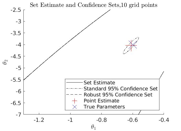
(a)

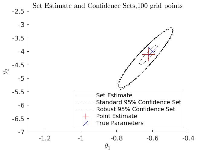
(b)

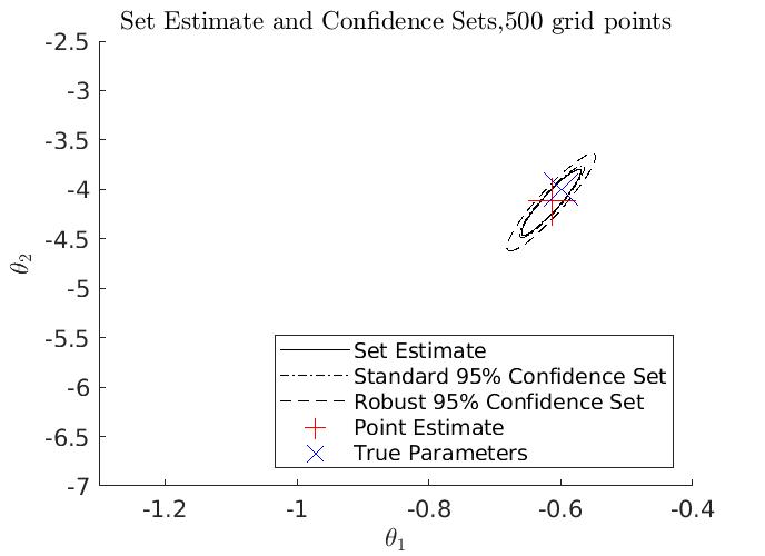
(c)

5 Conclusion

We develop an approach to estimation and inference in dynamic discrete choice models that directly accounts for error due to the use of approximate dynamic programming. We prove the validity of our approach and provide simulation evidence that our methodology is of practical use. Of course, our simulation results pertain to one particular model, and it is possible that the robust confidence sets are overly conservative in other settings. To better assess the practical efficacy of our methods we hope to implement the procedure on real data in future work.

The methodology detailed in the paper is very flexible in that it applies regardless of the approximation method used. It may be possible to refine our approach taking into account features of the specific approximate dynamic programming method used. It may also be possible to tighten our error bounds by incorporating information about the value function that can be derived analytically, for example, in some cases one can prove the value function is convex. This avenue may also be worth exploring in future research.

Appendix: Proofs

Proof Theorem 1.

By the definition of $T$ for any bounded functions $\tilde{V}$ and $\hat{V}$ that map from $\mathcal{S}\times\mathcal{D}$ to $\mathbb{R}$:

$$= T[\tilde{V}](s,d)-T[\tilde{V}](s^{\prime},d^{\prime})-\big{(}T[\hat{V}](s^{\prime},d^{\prime})-T[\hat{V}](s^{\prime},d^{\prime})\big{)}$$

$$= E[E[\max_{d^{\prime\prime}\in\mathcal{D}}\,u(S_{t+1},d^{\prime\prime})+\beta\tilde{V}(S_{t+1},d^{\prime\prime})+\epsilon_{t+1}(d^{\prime\prime})]|S_{t}=s,D_{t}=d]$$

$$- E[E[\max_{d^{\prime\prime}\in\mathcal{D}}\,u(s^{\prime},d^{\prime\prime})+\beta\tilde{V}(s^{\prime},d^{\prime\prime})+\epsilon_{t+1}(d^{\prime\prime})]|S_{t}=s^{\prime},D_{t}=d^{\prime}]$$

$$+ E[E[\max_{d^{\prime\prime}\in\mathcal{D}}\,u(S_{t+1},d^{\prime\prime})+\beta\hat{V}(S_{t+1},d^{\prime\prime})+\epsilon_{t+1}(d^{\prime\prime})]|S_{t}=s,D_{t}=d]$$

$$- E[E[\max_{d^{\prime\prime}\in\mathcal{D}}\,u(S_{t+1},d^{\prime\prime})+\beta\hat{V}(S_{t+1},d^{\prime\prime})+\epsilon_{t+1}(d^{\prime\prime})]|S_{t}=s^{\prime},D_{t}=d^{\prime}]$$

Because $\epsilon_{t+1}$ and $S_{t+1}$ are independent we can rewrite the right-hand side of the final equality above as an integral:

$$\int\bigg{(}E[\max_{d^{\prime\prime}\in\mathcal{D}}\,u(s^{\prime\prime},d^{\prime\prime})+\beta\tilde{V}(s^{\prime\prime},d^{\prime\prime})+\epsilon_{t}(d^{\prime\prime})]$$

$$-E[\max_{d^{\prime\prime}\in\mathcal{D}}\,u(s^{\prime\prime},d^{\prime\prime})+\beta\hat{V}(s^{\prime\prime},d^{\prime\prime})+\epsilon_{t}(d^{\prime\prime})]\bigg{)}d(F_{s,d}-F_{s^{\prime},d^{\prime}})$$

It is an elementary property of the total variation distance that for any bounded function $g:\mathcal{S}\to\mathbb{R}$:

$$\int g(s^{\prime\prime})d(F_{s,d}-F_{s^{\prime},d^{\prime}}) \leq \delta(F_{s,d},F_{s^{\prime},d^{\prime}})\big{(}\sup_{s\in\mathcal{S}}g(s)-\inf_{s\in\mathcal{S}}g(s)\big{)}$$

Since $u$, $\tilde{V}$, and $\hat{V}$ are bounded and $E[\max_{d\in\mathcal{D}}\epsilon_{t}(d)]<\infty$, $E[\max_{d\in\mathcal{D}}\,u(s,d)+\beta\tilde{V}(s,d)+\epsilon_{t}(d)]$ and $E[\max_{d\in\mathcal{D}}\,u(s,d)+\beta\hat{V}(s,d)+\epsilon_{t}(d)]$ are also uniformly bounded over $s\in\mathcal{S}$ and so applying the inequality above:

$$\int\bigg{(}E[\max_{d^{\prime\prime}\in\mathcal{D}}\,u(s^{\prime\prime},d^{\prime\prime})+\beta\tilde{V}(s^{\prime\prime},d^{\prime\prime})+\epsilon_{t}(d^{\prime\prime})]$$

$$-E[\max_{d^{\prime\prime}\in\mathcal{D}}\,u(s^{\prime\prime},d^{\prime\prime})+\beta\hat{V}(s^{\prime\prime},d^{\prime\prime})+\epsilon_{t}(d^{\prime\prime})]\bigg{)}d(F_{s,d}-F_{s^{\prime},d^{\prime}})$$

$$\leq \delta(F_{s,d},F_{s^{\prime},d^{\prime}})\sup_{s^{\prime\prime}\in\mathcal{S}}\bigg{(}E[\max_{d^{\prime\prime}\in\mathcal{D}}\,u(s^{\prime\prime},d^{\prime\prime})+\beta\tilde{V}(s^{\prime\prime},d^{\prime\prime})+\epsilon_{t}(d^{\prime\prime})]$$

$$-E[\max_{d^{\prime\prime}\in\mathcal{D}}\,u(s^{\prime\prime},d^{\prime\prime})+\beta\hat{V}(s^{\prime\prime},d^{\prime\prime})+\epsilon_{t}(d^{\prime\prime})]\bigg{)}$$

$$- \delta(F_{s,d},F_{s^{\prime},d^{\prime}})\inf_{s^{\prime\prime}\in\mathcal{S}}\bigg{(}E[\max_{d^{\prime\prime}\in\mathcal{D}}\,u(s^{\prime\prime},d^{\prime\prime})+\beta\tilde{V}(s^{\prime\prime},d^{\prime\prime})+\epsilon_{t}(d^{\prime\prime})]$$

$$-E[\max_{d^{\prime\prime}\in\mathcal{D}}\,u(s^{\prime\prime},d^{\prime\prime})+\beta\hat{V}(s^{\prime\prime},d^{\prime\prime})+\epsilon_{t}(d^{\prime\prime})]\bigg{)}$$

It is easy to see that:

$$\sup_{s\in\mathcal{S}}\bigg{(}E[\max_{d\in\mathcal{D}}\,u(s,d)+\beta\tilde{V}(s,d)+\epsilon_{t}(d)]$$

$$-E[\max_{d\in\mathcal{D}}\,u(s,d)+\beta\hat{V}(s,d)+\epsilon_{t}(d)]\bigg{)}$$

$$\leq \beta\sup_{s\in\mathcal{S}}\max_{d\in\mathcal{D}}\big{(}\tilde{V}(s,d)-\hat{V}(s,d)\big{)}$$

And:

$$\inf_{s\in\mathcal{S}}\bigg{(}E[\max_{d}\,u(s,d)+\beta\tilde{V}(s,d)+\epsilon_{t}(d)]$$

$$-E[\max_{d^{\prime\prime}}\,u(s,d)+\beta\hat{V}(s,d)+\epsilon_{t}(d)]\bigg{)}$$

$$\geq \beta\inf_{s}\min_{d\in\mathcal{D}}\big{(}\tilde{V}(s,d)-\hat{V}(s,d)\big{)}$$

Combining we get:

$$T[\tilde{V}](s,d)-T[\tilde{V}](s^{\prime},d^{\prime})-\big{(}T[\hat{V}](s^{\prime},d^{\prime})-T[\hat{V}](s^{\prime},d^{\prime})\big{)}$$

$$\leq \delta(F_{s,d},F_{s^{\prime},d^{\prime}})\beta\bigg{(}\sup_{s\in\mathcal{S}}\max_{d\in\mathcal{D}}\big{(}\tilde{V}(s,d)-\hat{V}(s,d)\big{)}-\inf_{s}\min_{d\in\mathcal{D}}\big{(}\tilde{V}(s,d)-\hat{V}(s,d)\big{)}\bigg{)}$$

$$= \delta(F_{s,d},F_{s^{\prime},d^{\prime}})\beta\sup_{s,s^{\prime}\in\mathcal{S},d,d^{\prime}\in\mathcal{D}}\big{|}\tilde{V}(s,d)-\tilde{V}(s^{\prime},d^{\prime})-\big{(}\hat{V}(s,d)-\hat{V}(s^{\prime},d^{\prime})\big{)}\big{|}$$

Since the same reasoning holds with $\tilde{V}$ and $\hat{V}$ switched we get:

$$\big{|}T[\tilde{V}](s,d)-T[\tilde{V}](s^{\prime},d^{\prime})-\big{(}T[\hat{V}](s^{\prime},d^{\prime})-T[\hat{V}](s^{\prime},d^{\prime})\big{)}\big{|}$$

$$\leq \delta(F_{s,d},F_{s^{\prime},d^{\prime}})\beta\sup_{s,s^{\prime}\in\mathcal{S},d,d^{\prime}\in\mathcal{D}}\big{|}\tilde{V}(s,d)-\tilde{V}(s^{\prime},d^{\prime})-\big{(}\hat{V}(s,d)-\hat{V}(s^{\prime},d^{\prime})\big{)}\big{|}$$

Now, $V$ is a fixed point of $T$ and it must be bounded because $u$ is bounded and $E[\max_{d\in\mathcal{D}}\epsilon_{t}(d)]<\infty$. Thus the above implies:

$$\big{|}T[\tilde{V}](s,d)-T[\tilde{V}](s^{\prime},d^{\prime})-\big{(}V(s^{\prime},d^{\prime})-V(s^{\prime},d^{\prime})\big{)}\big{|}$$ (4)

$$\leq \delta(F_{s,d},F_{s^{\prime},d^{\prime}})\beta\sup_{s,s^{\prime}\in\mathcal{S},d,d^{\prime}\in\mathcal{D}}\big{|}\tilde{V}(s,d)-\tilde{V}(s^{\prime},d^{\prime})-\big{(}V(s,d)-V(s^{\prime},d^{\prime})\big{)}\big{|}$$

Taking the supremum over both sides:

$$\sup_{s,s^{\prime}\in\mathcal{S},d,d^{\prime}\in\mathcal{D}}\big{|}T[\tilde{V}](s,d)-T[\tilde{V}](s^{\prime},d^{\prime})-\big{(}V(s^{\prime},d^{\prime})-V(s^{\prime},d^{\prime})\big{)}\big{|}$$

$$\leq \sup_{s,s^{\prime}\in\mathcal{S},d,d^{\prime}\in\mathcal{D}}\delta(F_{s,d},F_{s^{\prime},d^{\prime}})\beta\sup_{s,s^{\prime}\in\mathcal{S},d,d^{\prime}\in\mathcal{D}}\big{|}\tilde{V}(s,d)-\tilde{V}(s^{\prime},d^{\prime})-\big{(}V(s,d)-V(s^{\prime},d^{\prime})\big{)}\big{|}$$

By the reverse triangle inequality:

$$\sup_{s,s^{\prime}\in\mathcal{S},d,d^{\prime}\in\mathcal{D}}\big{|}\tilde{V}(s,d)-\tilde{V}(s^{\prime},d^{\prime})-\big{(}V(s^{\prime},d^{\prime})-V(s^{\prime},d^{\prime})\big{)}\big{|}$$

$$- \sup_{s,s^{\prime}\in\mathcal{S},d,d^{\prime}\in\mathcal{D}}\big{|}T[\tilde{V}](s,d)-T[\tilde{V}](s^{\prime},d^{\prime})-\big{(}\tilde{V}(s^{\prime},d^{\prime})-\tilde{V}(s^{\prime},d^{\prime})\big{)}\big{|}$$

$$\leq \sup_{s,s^{\prime}\in\mathcal{S},d,d^{\prime}\in\mathcal{D}}\delta(F_{s,d},F_{s^{\prime},d^{\prime}})\beta\sup_{s,s^{\prime}\in\mathcal{S},d,d^{\prime}\in\mathcal{D}}\big{|}\tilde{V}(s,d)-\tilde{V}(s^{\prime},d^{\prime})-\big{(}V(s,d)-V(s^{\prime},d^{\prime})\big{)}\big{|}$$

Since $\delta(F_{s,d},F_{s^{\prime},d^{\prime}})\beta\leq\beta<1$ we can solve to get:

$$\sup_{s,s^{\prime}\in\mathcal{S},d,d^{\prime}\in\mathcal{D}}\big{|}\tilde{V}(s,d)-\tilde{V}(s^{\prime},d^{\prime})-\big{(}V(s^{\prime},d^{\prime})-V(s^{\prime},d^{\prime})\big{)}\big{|}$$ (5)

$$\leq \frac{1}{1-\sup_{s,s^{\prime}\in\mathcal{S},d,d^{\prime}\in\mathcal{D}}\delta(F_{s,d},F_{s^{\prime},d^{\prime}})\beta}$$

$$\times \sup_{s,s^{\prime}\in\mathcal{S},d,d^{\prime}\in\mathcal{D}}\big{|}T[\tilde{V}](s,d)-T[\tilde{V}](s^{\prime},d^{\prime})-\big{(}\tilde{V}(s^{\prime},d^{\prime})-\tilde{V}(s^{\prime},d^{\prime})\big{)}\big{|}$$

Also by the triangle inequality:

$$|\tilde{V}(s,d)-\tilde{V}(s^{\prime},d^{\prime})-[V(s,d)-V(s^{\prime},d^{\prime})]|$$

$$\leq |T[\tilde{V}](s,d)-T[\tilde{V}](s^{\prime},d^{\prime})-[\tilde{V}(s,d)-\tilde{V}(s^{\prime},d^{\prime})]|$$

$$+ |T[\tilde{V}](s,d)-T[\tilde{V}](s^{\prime},d^{\prime})-[V(s,d)-V(s^{\prime},d^{\prime})]|$$

Substituting using (4) we get:

$$|\tilde{V}(s,d)-\tilde{V}(s^{\prime},d^{\prime})-[V(s,d)-V(s^{\prime},d^{\prime})]|$$

$$\leq |T[\tilde{V}](s,d)-T[\tilde{V}](s^{\prime},d^{\prime})-[\tilde{V}(s,d^{\prime})-\tilde{V}(s^{\prime},d^{\prime})]|$$

$$+ \delta(F_{s,d},F_{s^{\prime},d^{\prime}})\beta\sup_{s,s^{\prime}\in\mathcal{S},d,d^{\prime}\in\mathcal{D}}\big{|}\tilde{V}(s,d)-\tilde{V}(s^{\prime},d^{\prime})-\big{(}V(s,d)-V(s^{\prime},d^{\prime})\big{)}\big{|}$$

And so from (5):

$$|\tilde{V}(s,d)-\tilde{V}(s^{\prime},d^{\prime})-[V(s,d)-V(s^{\prime},d^{\prime})]|$$

$$\leq |T[\tilde{V}](s,d)-T[\tilde{V}](s^{\prime},d^{\prime})-[\tilde{V}(s,d^{\prime})-\tilde{V}(s^{\prime},d^{\prime})]|$$

$$+ \bigg{(}\frac{\delta(F_{s,d},F_{s^{\prime},d^{\prime}})\beta}{1-\sup_{s,s^{\prime}\in\mathcal{S},d,d^{\prime}\in\mathcal{D}}\delta(F_{s,d},F_{s^{\prime},d^{\prime}})\beta}$$

$$\times \sup_{s,s^{\prime}\in\mathcal{S},d,d^{\prime}\in\mathcal{D}}\big{|}T[\tilde{V}](s,d)-T[\tilde{V}](s^{\prime},d^{\prime})-\big{(}\tilde{V}(s^{\prime},d^{\prime})-\tilde{V}(s^{\prime},d^{\prime})\big{)}\big{|}\bigg{)}$$

Taking the supremum over the RHS we get:

$$|\tilde{V}(s,d)-\tilde{V}(s^{\prime},d^{\prime})-[V(s,d)-V(s^{\prime},d^{\prime})]|$$

$$\leq \bigg{(}\frac{1-\sup_{s,s^{\prime}\in\mathcal{S},d,d^{\prime}\in\mathcal{D}}\delta(F_{s,d},F_{s^{\prime},d^{\prime}})\beta+\delta(F_{s,d},F_{s^{\prime},d^{\prime}})\beta}{1-\sup_{s,s^{\prime}\in\mathcal{S},d,d^{\prime}\in\mathcal{D}}\delta(F_{s,d},F_{s^{\prime},d^{\prime}})\beta}$$

$$\times \sup_{s,s^{\prime}\in\mathcal{S},d,d^{\prime}\in\mathcal{D}}\big{|}T[\tilde{V}](s,d)-T[\tilde{V}](s^{\prime},d^{\prime})-\big{(}\tilde{V}(s^{\prime},d^{\prime})-\tilde{V}(s^{\prime},d^{\prime})\big{)}\big{|}\bigg{)}$$

The conclusion then follows immediately. ∎

Proof Theorem 2.

First we show that for any $s,s^{\prime}\in\mathcal{S}$ and $d,d^{\prime}\in\mathcal{D}$:

$$|T\tilde{V}(s,d)-T\tilde{V}(s^{\prime},d^{\prime})|\leq\delta(F_{s,d},F_{s^{\prime},d^{\prime}})\bar{b}_{\tilde{V}}$$

By the definition of $T$:

$$T[\tilde{V}](s,d)-T[\tilde{V}](s^{\prime},d^{\prime})$$

$$= E[E[\max_{d^{\prime\prime}\in\mathcal{D}}\,u(S_{t+1},d^{\prime\prime})+\beta\tilde{V}(S_{t+1},d^{\prime\prime})+\epsilon_{t+1}(d^{\prime\prime})]|S_{t}=s,D_{t}=d]$$

$$- E[E[\max_{d^{\prime\prime}\in\mathcal{D}}\,u(s^{\prime},d^{\prime\prime})+\beta\tilde{V}(s^{\prime},d^{\prime\prime})+\epsilon_{t+1}(d^{\prime\prime})]|S_{t}=s^{\prime},D_{t}=d^{\prime}]$$

Using independence of $\epsilon_{t+1}$ and $S_{t+1}$ the right-hand side above is equal to:

$$\int E[\max_{d^{\prime\prime}\in\mathcal{D}}\,u(s^{\prime\prime},d^{\prime\prime})+\beta\tilde{V}(s^{\prime\prime},d^{\prime\prime})+\epsilon_{t}(d^{\prime\prime})]d(F_{s,d}-F_{s^{\prime},d^{\prime}})$$

As in the proof of Theorem 1 we can apply elementary properties of the total variation distance to get:

$$\int g(x)d(F_{s,d}-F_{s^{\prime},d^{\prime}})\leq\delta(F_{s,d},F_{s^{\prime},d^{\prime}})\sup_{x,x^{\prime}\in\mathcal{S}(s,d)\cup\mathcal{S}(s^{\prime},d^{\prime})}g(x)-g(x^{\prime})$$

$$\int E[\max_{d^{\prime\prime}\in\mathcal{D}}\,u(s^{\prime\prime},d^{\prime\prime})+\beta\tilde{V}(s^{\prime\prime},d^{\prime\prime})+\epsilon_{t}(d^{\prime\prime})]d(F_{s,d}-F_{s^{\prime},d^{\prime}})$$

$$\leq \delta(F_{s,d},F_{s^{\prime},d^{\prime}})\bigg{(}\sup_{s^{\prime}\in\mathcal{S}}E[\max_{d^{\prime\prime}\in\mathcal{D}}\,u(s^{\prime\prime},d^{\prime\prime})+\beta\tilde{V}(s^{\prime\prime},d^{\prime\prime})+\epsilon_{t}(d^{\prime\prime})]$$

$$-\inf_{s^{\prime}\in\mathcal{S}}E[\max_{d^{\prime\prime}\in\mathcal{D}}\,u(s^{\prime\prime},d^{\prime\prime})+\beta\tilde{V}(s^{\prime\prime},d^{\prime\prime})+\epsilon_{t}(d^{\prime\prime})]\bigg{)}$$

$$= \delta(F_{s,d},F_{s^{\prime},d^{\prime}})\bigg{(}\sup_{s^{\prime},s\in\mathcal{S}}E[\max_{d^{\prime\prime}\in\mathcal{D}}\,u(s^{\prime\prime},d^{\prime\prime})+\beta\tilde{V}(s^{\prime\prime},d^{\prime\prime})+\epsilon_{t}(d^{\prime\prime})]$$

$$-E[\max_{d^{\prime\prime}\in\mathcal{D}}\,u(s^{\prime\prime},d^{\prime\prime})+\beta\tilde{V}(s^{\prime\prime},d^{\prime\prime})+\epsilon_{t}(d^{\prime\prime})]\bigg{)}$$

It is easy to see that for any $s^{\prime}\in\mathcal{S}$:

$$E[\max_{d\in\mathcal{D}}\,u(s,d)+\beta\tilde{V}(s,d)+\epsilon_{t}(d)]-E[\max_{d^{\prime}\in\mathcal{D}}\,u(s^{\prime},d)+\beta\tilde{V}(s^{\prime},d)+\epsilon_{t}(d)]\bigg{)}$$

$$\leq \max_{d\in\mathcal{D}}\,\big{(}u(s,d)+\beta\tilde{V}(s,d)-u(s^{\prime},d)+\beta\tilde{V}(s^{\prime},d)\big{)}$$

And so in all:

$$T[\tilde{V}](s,d)-T[\tilde{V}](s^{\prime},d^{\prime})$$

$$\leq \delta(F_{s,d},F_{s^{\prime},d^{\prime}})\sup_{s,s^{\prime}\in\mathcal{S},d\in\mathcal{D},}\,\big{(}u(s,d)+\beta\tilde{V}(s,d)-u(s^{\prime},d)+\beta\tilde{V}(s^{\prime},d)\big{)}$$

$$= \delta(F_{s,d},F_{s^{\prime},d^{\prime}})\big{|}\sup_{s,s^{\prime}\in\mathcal{S},d\in\mathcal{D},}\,\big{(}u(s,d)+\beta\tilde{V}(s,d)-u(s^{\prime},d)+\beta\tilde{V}(s^{\prime},d)\big{)}\big{|}$$

By symmetry:

$$|T[\tilde{V}](s,d)-T[\tilde{V}](s^{\prime},d^{\prime})|$$

$$\leq \delta(F_{s,d},F_{s^{\prime},d^{\prime}})\big{|}\sup_{s,s^{\prime}\in\mathcal{S},d\in\mathcal{D},}\,\big{(}u(s,d)+\beta\tilde{V}(s,d)-u(s^{\prime},d)+\beta\tilde{V}(s^{\prime},d)\big{)}\big{|}$$

$$= \delta(F_{s,d},F_{s^{\prime},d^{\prime}})\bar{b}_{\tilde{V}}$$

Now adding and subtracting terms, for any $(s^{*},d^{*}),(s^{**},d^{**})\in\mathcal{A}$:

$$T[\tilde{V}](s,d)-T[\tilde{V}](s^{\prime},d^{\prime})-[\tilde{V}(s,d)-\tilde{V}(s^{\prime},d^{\prime})]$$

$$= T[\tilde{V}](s^{*},d^{*})+T[\tilde{V}](s,d)-T[\tilde{V}](s^{*},d^{*})$$

$$- T[\tilde{V}](s^{**},d^{**})+T[\tilde{V}](s^{**},d^{**})-T[\tilde{V}](s^{\prime},d^{\prime})$$

$$- [\tilde{V}(s,d)-\tilde{V}(s^{\prime},d^{\prime})]$$

$$\leq T[\tilde{V}](s^{*},d^{*})+|T[\tilde{V}](s,d)-T[\tilde{V}](s^{*},d^{*})|$$

$$- T[\tilde{V}](s^{**},d^{**})+|T[\tilde{V}](s^{\prime},d^{\prime})-T[\tilde{V}](s^{**},d^{**})|$$

$$- [\tilde{V}(s,d)-\tilde{V}(s^{\prime},d^{\prime})]$$

Using the bound we derived earlier we get from the above:

$$T[\tilde{V}](s,d)-T[\tilde{V}](s^{\prime},d^{\prime})-[\tilde{V}(s,d)-\tilde{V}(s^{\prime},d^{\prime})]$$

$$\leq T[\tilde{V}](s^{*},d^{*})+\delta(F_{s,d},F_{s^{*},d^{*}})\bar{b}_{\tilde{V}}$$

$$- T[\tilde{V}](s^{**},d^{**})+\delta(F_{s^{\prime},d^{\prime}},F_{s^{**},d^{**}})\bar{b}_{\tilde{V}}$$

$$- [\tilde{V}(s,d)-\tilde{V}(s^{\prime},d^{\prime})]$$

Since the above holds for any $(s^{*},d^{*}),(s^{**},d^{**})\in\mathcal{A}$ we can choose these to minimize it:

$$T[\tilde{V}](s,d)-T[\tilde{V}](s^{\prime},d^{\prime})-[\tilde{V}(s,d)-\tilde{V}(s^{\prime},d^{\prime})]$$

$$\leq \min_{(s^{*},d^{*})\in\mathcal{A}}\{T[\tilde{V}](s^{*},d^{*})+\delta(F_{s,d},F_{s^{*},d^{*}})\bar{b}_{\tilde{V}}\}$$

$$- \max_{(s^{*},d^{*})\in\mathcal{A}}\{T[\tilde{V}](s^{*},d^{*})-\delta(F_{s^{\prime},d^{\prime}},F_{s^{*},d^{*}})\bar{b}_{\tilde{V}}\}$$

$$- [\tilde{V}(s,d)-\tilde{V}(s^{\prime},d^{\prime})]$$

Taking the supremum of both sides above over $s,s^{\prime}\in\mathcal{S}$ and $d,d^{\prime}\in\mathcal{D}$ and noting that by symmetry:

$$\sup_{s,s^{\prime}\in\mathcal{S},d,d^{\prime}\in\mathcal{D}}T[\tilde{V}](s,d)-T[\tilde{V}](s^{\prime},d^{\prime})-[\tilde{V}(s,d)-\tilde{V}(s^{\prime},d^{\prime})]>0$$

We get the result. ∎

Proof Theorem 3.

Let $B$ be defined by:

$$B=\sup_{s,s^{\prime}\in S,d,d^{\prime}\in D}|[T[\tilde{V}](s^{\prime},d^{\prime})-T[\tilde{V}](s,d)]-[\tilde{V}(s^{\prime},d^{\prime})-\tilde{V}(s,d)]]|$$

Fix some $\tau>0$. Recall $\underline{B}$ is defined by:

$$\underline{B} =\max_{(s,d),(s^{\prime},d^{\prime})\in\mathcal{A}}\{|T[\tilde{V}](s,d)-T[\tilde{V}](s^{\prime},d^{\prime})-[\tilde{V}(s,d)-\tilde{V}(s^{\prime},d^{\prime})]|\}$$

$$=\max_{(s,d)\in\mathcal{A}}\big{(}T[\tilde{V}](s,d)-\tilde{V}(s,d)\big{)}-\min_{(s^{\prime},d^{\prime})\in\mathcal{A}}\big{(}T[\tilde{V}](s^{\prime},d^{\prime})-\tilde{V}(s^{\prime},d^{\prime})\big{)}$$

A linear combination of two uniformly continuous functions is also uniformly continuous, and so $s\mapsto T[\tilde{V}](s,d)-\tilde{V}(s,d)$ is uniformly continuous for each $d\in\mathcal{D}$, there must exist some $\eta_{1}>0$ so that for every $d\in\mathcal{D}$:

$$\sup_{s,s^{\prime}\in\mathcal{S}:||s-s^{\prime}||\leq\eta}|\big{(}T[\tilde{V}](s,d)-\tilde{V}(s,d)\big{)}-\big{(}T[\tilde{V}](s^{\prime},d)-\tilde{V}(s^{\prime},d)\big{)}|\leq\frac{1}{4}\tau$$

So suppose that for any $d\in\mathcal{D}$ and $s\in\mathcal{S}$ there is an $s^{\prime}$ with $||s-s^{\prime}||\leq\eta_{1}$ and $(s^{\prime},d)\in\mathcal{A}$, then:

$$\sup_{s\in\mathcal{S},d\in\mathcal{D}}\min_{s^{\prime}\in\mathcal{S}:(s^{\prime},d)\in\mathcal{A}}|\big{(}T[\tilde{V}](s,d)-\tilde{V}(s,d)\big{)}-\big{(}T[\tilde{V}](s^{\prime},d)-\tilde{V}(s^{\prime},d)\big{)}|\leq\frac{1}{4}\tau$$

And so:

$$\sup_{s\in\mathcal{S},d\in\mathcal{D}}\big{(}T[\tilde{V}](s,d)-\tilde{V}(s,d)\big{)}-\max_{(s,d)\in\mathcal{A}}\big{(}T[\tilde{V}](s,d)-\tilde{V}(s,d)\big{)}\leq\frac{1}{4}\tau$$

And:

$$\inf_{s\in\mathcal{S},d\in\mathcal{D}}\big{(}T[\tilde{V}](s,d)-\tilde{V}(s,d)\big{)}-\min_{(s,d)\in\mathcal{A}}\big{(}T[\tilde{V}](s,d)-\tilde{V}(s,d)\big{)}\leq\frac{1}{4}\tau$$

And so:

$$B-\underline{B}\leq\frac{1}{2}\tau$$

Next, recall the definition of $\bar{B}$:

$$\bar{B}= \sup_{s,s^{\prime}\in S,d,d^{\prime}\in D}\bigg{[}\min_{(s^{*},d^{*})\in\mathcal{A}}\{T[\tilde{V}](s^{*},d^{*})+\delta(F_{s,d},F_{s^{*},d^{*}})\bar{b}_{\tilde{V}}\}$$

$$-\max_{(s^{*},d^{*})\in\mathcal{A}}\{T[\tilde{V}](s^{*},d^{*})-\delta(F_{s^{\prime},d^{\prime}},F_{s^{*},d^{*}})\bar{b}_{\tilde{V}}\}-[\tilde{V}(s,d)-\tilde{V}(s^{\prime},d^{\prime})]\bigg{]}$$

$$= \sup_{s,s^{\prime}\in S,d,d^{\prime}\in D}\bigg{[}\min_{(s^{*},d^{*})\in\mathcal{A}}\big{\{}T[\tilde{V}](s^{*},d^{*})-T[\tilde{V}](s,d)$$

$$+\big{(}\delta(F_{s,d},F_{s^{*},d^{*}})-\delta(F_{s,d},F_{s,d})\big{)}\bar{b}_{\tilde{V}}\big{\}}$$

$$+\min_{(s^{*},d^{*})\in\mathcal{A}}\big{\{}T[\tilde{V}](s^{\prime},d^{\prime})-T[\tilde{V}](s^{*},d^{*})$$

$$+\big{(}\delta(F_{s^{\prime},d^{\prime}},F_{s^{*},d^{*}})-\delta(F_{s^{\prime},d^{\prime}},F_{s^{\prime},d^{\prime}})\big{)}\bar{b}_{\tilde{V}}\big{\}}$$

$$-[\big{(}\tilde{V}(s,d)-T[\tilde{V}](s,d)\big{)}+\big{(}T[\tilde{V}](s^{\prime},d^{\prime})-\tilde{V}(s^{\prime},d^{\prime})\big{)}]\bigg{]}$$

Where we have used that $\delta(F_{s,d},F_{s,d})=\delta(F_{s^{\prime},d^{\prime}},F_{s^{\prime},d^{\prime}})=0$. By the triangle inequality, the RHS of the final equality above is bounded by:

$$2\sup_{s\in S,d\in D}\min_{(s^{*},d^{*})\in\mathcal{A}}|T[\tilde{V}](s^{*},d^{*})-T[\tilde{V}](s,d)+\big{(}\delta(F_{s,d},F_{s^{*},d^{*}})-\delta(F_{s,d},F_{s,d})\big{)}\bar{b}_{\tilde{V}}|$$

$$+ B$$

A linear combination of two uniformly continuous functions is uniformly continuous and so $(s,s^{\prime})\mapsto T[\tilde{V}](s,d)+\delta(F_{s^{\prime},d},F_{s,d})\bar{b}_{\tilde{V}}$ is uniformly continuous for all $d\in\mathcal{D}$. It follows that for some $\eta_{2}>0$:

$$\sup_{s,s^{\prime}\in S:||s-s^{\prime}||\leq\eta}|T[\tilde{V}](s^{\prime},d)-T[\tilde{V}](s,d)+\big{(}\delta(F_{s,d},F_{s^{\prime},d})-\delta(F_{s,d},F_{s,d})\big{)}\bar{b}_{\tilde{V}}|\leq\frac{1}{4}\tau$$

For all $d\in\mathcal{D}$. So suppose that for any $d\in\mathcal{D}$ and $s\in\mathcal{S}$ there is an $s^{\prime}$ with $||s-s^{\prime}||\leq\eta_{2}$ and $(s^{\prime},d)\in\mathcal{A}$, then:

$$\sup_{s\in S,d\in D}\min_{(s^{*},d^{*})\in\mathcal{A}}|T[\tilde{V}](s^{*},d^{*})-T[\tilde{V}](s,d)+\big{(}\delta(F_{s,d},F_{s^{*},d^{*}})-\delta(F_{s,d},F_{s,d})\big{)}\bar{b}_{\tilde{V}}|\leq\frac{1}{2}\tau$$

And so:

$$\bar{B}-B\leq\frac{1}{2}\tau$$

Finally, for dense enough $\mathcal{A}$, for any $d\in\mathcal{D}$ and $s\in\mathcal{S}$ there is an $s^{\prime}$ with $||s-s^{\prime}||\leq\min\{\eta_{1},\eta_{2}\}$ and $(s^{\prime},d)\in\mathcal{A}$ and hence:

$$\bar{B}-\underline{B}\leq\tau$$

$\tau$ was chosen arbitrarily and so as the density of $\mathcal{A}$ grows to infinity $\bar{B}-\underline{B}\to 0$. ∎

References

• Abbring & ystein Daljord, (2020) Abbring, & ystein Daljord. 2020. Identifying the Discount Factor in Dynamic Discrete Choice Models. Quantitive Economics.
• Aguirregabiria & Mira, (2002) Aguirregabiria, Victor, & Mira, Pedro. 2002. Swapping the Nested Fixed Point Algorithm: A Class of Estimators for Discrete Markov Decision Models. Econometrica, 70, 1519–1543.
• Aguirregabiria & Mira, (2007) Aguirregabiria, Victor, & Mira, Pedro. 2007. Sequential Estimation of Dynamic Discrete Games. Econometrica, 75, 1–53.
• Arcidiacono et al., (2013) Arcidiacono, Peter, Bayer, Patrick, Bugni, Federico A., & James, Jonathan. 2013. Approximating High-dimensional Dynamic Models: Sieve Value Function Iteration.
• Bajari et al., (2007) Bajari, Patrick, Benkard, C. Lanier, & Levin, Jonathan. 2007. Estimating Dynamic Models of Imperfect Competition. Econometrica, 75, 1331–1370.
• Bellman, (1957) Bellman, R. 1957. Dynamic Programming. Princeton University Press.
• Bellman et al., (1963) Bellman, Richard, Kalaba, Robert, & Kotkin, Bella. 1963. Polynomial Approximation–A New Computational Technique in Dynamic Programming: Allocation Processes. Mathematics of Computation, 17, 155.
• Hotz & Miller, (1993) Hotz, V. Joseph, & Miller, Robert A. 1993. Conditional Choice Probabilities and the Estimation of Dynamic Models. Review of Economic Studies, 60, 497.
• Keane & Wolpin, (1992) Keane, Michael P., & Wolpin, Kenneth I. 1992. The Solution and Estimation of Discrete Choice Dynamic Programming Models by Simulation and Interpolation: Monte Carlo Evidence. The Review of Economics and Statistics, 76(4), 684–672.
• Keane et al., (2011) Keane, Michael P., Todd, Petra E., & Wolpin, Kenneth I. 2011. The Structural Estimation of Behavioral Models: Discrete Choice Dynamic Programming Methods and Applications, Chapter 4, Handbook of Labor Economics Volume 4a.
• Magnac & Thesmar, (2002) Magnac, Thierry, & Thesmar, David. 2002. Identifying dynamic discrete decision processes. Econometrica. Journal of the Econometric Society, 70(2), 801–816.
• Norets, (2012) Norets, Andriy. 2012. Estimation of Dynamic Discrete Choice Models Using Artificial Neural Network Approximations. Econometric Reviews, 31, 84–106.
• Rust, (1987) Rust, John. 1987. Optimal Replacement of GMC Bus Engines: An Empirical Model of Harold Zurcher. Econometrica, 55, 999.
• Su & Judd, (2012) Su, Che-Lin, & Judd, Kenneth L. 2012. Constrained Optimization Approaches to Estimation of Structural Models. Econometrica.
• Wolpin, (1984) Wolpin, Kenneth I. 1984. An Estimable Dynamic Stochastic Model of Fertility and Child Mortality. Journal of Political Economy, 92, 852–874.