Knowledge Distillation for BERT Unsupervised Domain Adaptation

Abstract

A pre-trained language model, BERT, has brought significant performance improvements across a range of natural language processing tasks. Since the model is trained on a large corpus of diverse topics, it shows robust performance for domain shift problems in which data distributions at training (source data) and testing (target data) differ while sharing similarities. Despite its great improvements compared to previous models, it still suffers from performance degradation due to domain shifts. To mitigate such problems, we propose a simple but effective unsupervised domain adaptation method, adversarial adaptation with distillation (AAD), which combines the adversarial discriminative domain adaptation (ADDA) framework with knowledge distillation. We evaluate our approach in the task of cross-domain sentiment classification on 30 domain pairs, advancing the state-of-the-art performance for unsupervised domain adaptation in text sentiment classification.

1 Introduction

The cost of creating labeled data for a new machine learning task is often a major obstacle to the application of machine learning algorithms. In particular, the obstacle is more restrictive for deep learning architectures that require huge datasets to learn a good representation. Even if enough data are available for a particular problem, performance may degrade due to distribution changes in training, testing, and actual service.

Domain adaptation is a way for machine learning models trained on source domain data to maintain good performance on target domain data. In domain adaptation methods, semi-supervised methods require a small amount of labeling in a target domain while unsupervised methods do not. Although semi-supervised methods may provide better performance, unsupervised domain adaptation methods are more often noticeable and attractive because of the high cost of data annotation depending on the new domain.

With the development of deep neural networks, unsupervised domain adaptation methods have focused on learning to map source and target data into a common feature space. This is usually accomplished by optimizing the representation to minimize some measure of domain shifts such as maximum mean discrepancy (Tzeng et al., 2014) or correlation distances (Sun et al., 2016; Sun & Saenko, 2016). Particularly, adversarial domain adaptation methods have become more popular in recent years, seeking to minimize domain discrepancy distance through an adversarial objective (Ganin et al., 2016; Tzeng et al., 2017).

However, these methods appear to be unfavorable when applied to large-scale and pre-trained language models such as BERT (Devlin et al., 2018). Pre-trained language models (Peters et al., 2018; Radford, 2018; Devlin et al., 2018; Yang et al., 2019) have brought tremendous performance improvements in numerous natural language processing (NLP) tasks. With respect to domain shift issues, showing robust performance and outperforming existing models without domain adaptation, they still suffer from performance degradation due to domain shifts.

In this paper, we propose a novel adversarial domain adaptation method for pre-trained language models, called adversarial adaptation with distillation (AAD). This work is done on top of the framework, called adversarial discriminative domain adaptation (ADDA), proposed by Tzeng et al. (Tzeng et al., 2017). We observe that a catastrophic forgetting (Kirkpatrick et al., 2016) occurs when the ADDA framework is applied to the BERT model as opposed to when applied to deep convolutional neural networks. In ADDA, the fine-tuned source model is used as an initialization to prevent the target model from learning degenerate solutions because the target model is trained without label information. Unfortunately, this method alone does not prevent a catastrophic forgetting in BERT, resulting in random classification performance. To overcome this problem, we adopt the knowledge distillation method (Hinton et al., 2015), which is mainly used to improve the performance of a smaller model by transferring knowledge from a large model. We found that this method can serve as a regularization to maintain the information learned by the source data while enabling the resulting model to be domain adaptive and to avoid overfitting.

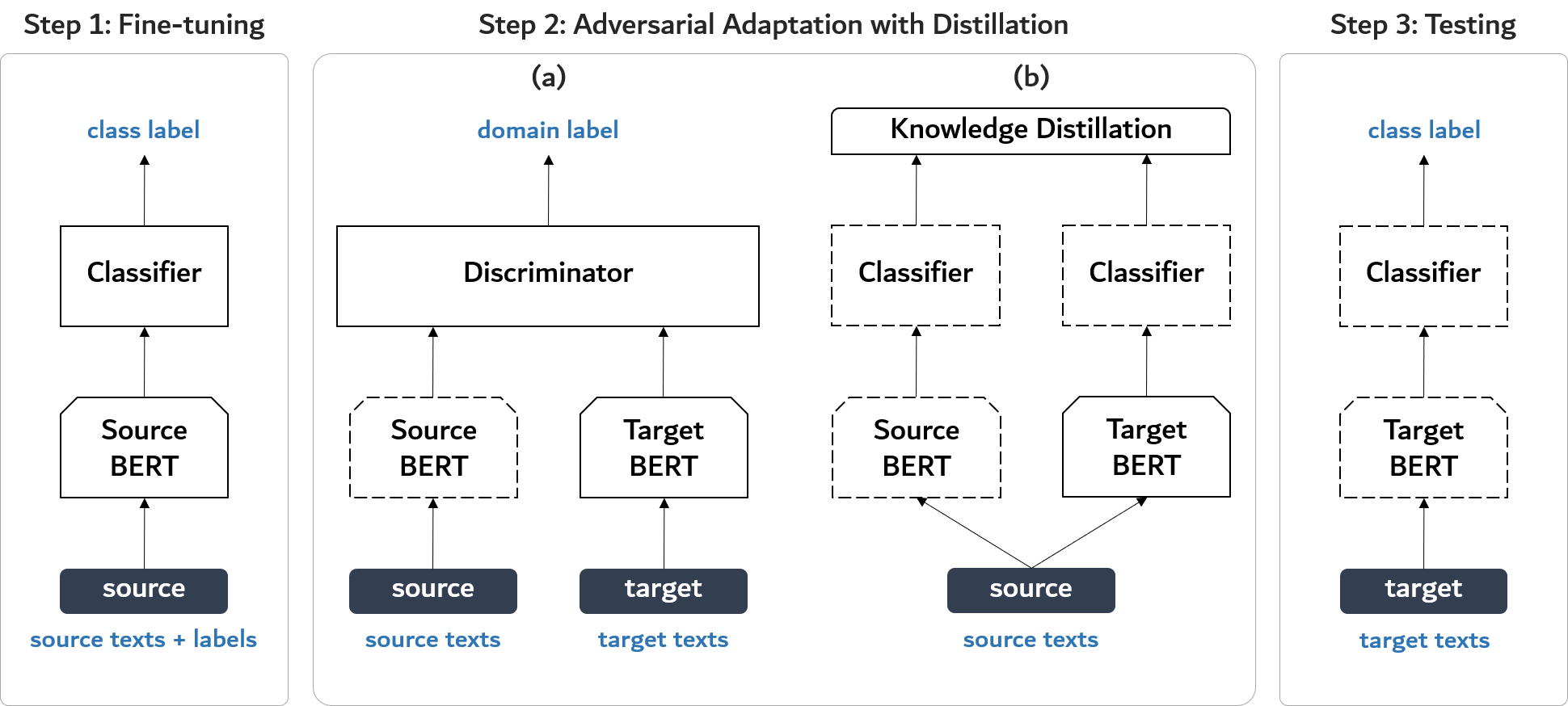
Figure 1: An overview of Adversarial Adaptation with Distillation. In Step 1, we first fine-tune a source BERT and a classifier on source labeled data. Next, in Step 2, after initializing the target BERT with weights of the fine-tuned source BERT, we perform adversarial learning and knowledge distillation simultaneously on the target BERT. Dashed line indicates fixed model parameters. Finally, in Step 3, the knowledge-distilled target BERT and the classifier predict class labels

2 Related Work

2.1 Unsupervised Domain Adaptation

Recently a large number of unsupervised domain adaptation methods have been studied. We present details of the studies that are most relevant to our paper. Recent studies have focused on transferring deep neural network representations learned from labeled source data to unlabeled target data.

Deep Domain Confusion (DDC) (Tzeng et al., 2014) introduces an adaptation layer to minimize Maximum Mean Discrepancy (MMD) in addition to classification loss on source data while the Deep Adaptation Network (DAN) (Long et al., 2015) applies multiple kernels to multiple layers. The deep Correlation Alignment (deep CORAL) (Sun & Saenko, 2016) minimizes the difference in second-order statistics between the source and target representations.

More recently, adversarial methods to minimize domain shifts have received much attention. The Domain Adversarial Neural Network (DANN) (Ganin et al., 2016) introduces a domain binary classification with a gradient reversal layer to train in the presence of domain confusion. Other studies have explored generative methods using Generative Adversarial Networks (GANs) (Goodfellow et al., 2014). A coupled generative adversarial network (CoGAN) (Liu & Tuzel, 2016) learns a joint distribution from the source and the target data with weight sharing constraints. Cycle-Consistent Adversarial Domain Adaptation (CyCADA) (Hoffman et al., 2018) uses cycle and semantic consistency for multi-level adaptation.

ADDA (Tzeng et al., 2017) was proposed as an adversarial framework that includes discriminative modeling, untied weight sharing, and a GAN-based loss. The source encoder is first trained with labeled source data and the weights are copied to the target encoder. Then, the target encoder and discriminator are alternately optimized in a two-player game like the original GAN setting. The discriminator learns to distinguish the target representations from the source representations while the encoder learns to trick the discriminator. Chadha et al. (Chadha & Andreopoulos, 2018) improved the ADDA framework by modifying the discriminator to jointly predict the source labels and distinguish inputs from the target domain as semi-supervised GANs (Kumar et al., 2017). Our study is similar to the work by Chadha et al. (2018) in that it also uses source information in the adversarial adaptation step. However, the difference is that the use of knowledge distillation, rather than the direct use of the source label, is the means to employ the source information in the network.

Besides, several unsupervised domain adaptation methods designed for NLP have also been proposed. Structural Corresponding Learning (SCL) (Blitzer et al., 2006) identifies correspondences among features from different domains by modeling their correlations with pivot features. Neural SCL (Ziser & Reichart, 2017) incorporates ideas of SCL and autoencoder neural networks. The Pivot Based Language Model (PBLM) (Ziser & Reichart, 2018) also combines the pivot-based idea of SCL with neural network based language modeling.

2.2 Knowledge Distillation

Knowledge Distillation (Hinton et al., 2015) (KD) is originally a model compression technique that aims to train a compact model (student) so that the knowledge of a well-trained larger model (teacher) is transferred to the student model. KD can be formulated by minimizing the following objective function

$$\mathcal{L}_{KD}=t^{2}\times\sum_{k}{-\textrm{softmax}(\boldsymbol{z}_{k}^{T}/t)\times\log(\textrm{softmax}(\boldsymbol{z}_{k}^{S}/t))}$$ (1)

where $\boldsymbol{z}^{S}$ and $\boldsymbol{z}^{T}$ are the logits predicted by the student and the teacher, respectively, and temperature value $t$ controls the degree of knowledge transfer. Equation 1 can be derived from the Kullback-Leibler (KL) divergence of the predicted distribution by the teacher from the predicted distribution by the student since the teacher model is fixed during training.

In supervised learning, the standard training objective is to minimize the cross-entropy between the distribution of the model’s predicted probability and that of one-hot-encoded labels’ true probability. However, this objective is prone to result in overfitting with repeated training epochs. Since a larger value for $t$ produces a softer probability distribution, knowledge distillation can mitigate this problem when incorporated with domain adaptation methods.

2.3 Bidirectional Encoder Representations from Transformers

BERT is a self-supervised approach for pre-training a deep transformer encoder (Vaswani et al., 2017). The BERT model is trained on a large corpus using masked language modeling and next sentence prediction. It has shown strong performance gains in many NLP tasks, and several variants have been proposed such as spanBERT (Joshi et al., 2019), distilBERT (Sanh et al., 2019), and RoBERTa (Liu et al., 2019). In this experiments, we use BERT, distilBERT and RoBERTa to evaluate our approach.

3 Adversarial Adaptation with Distillation

In this section, we introduce our unsupervised domain adaptation method, adversarial adaptation with distillation, which combines the ADDA framework (Tzeng et al., 2017) with knowledge distillation. We illustrate the proposed method in Figure 1.

Let us assume labeled source texts are given, $\mathbf{X}_{S}=\{(\boldsymbol{x}_{s}^{i})\}_{i=0}^{N_{s}}$, $\mathbf{y}_{S}=\{(y_{s}^{i})\}_{i=0}^{N_{s}}$ with $(\boldsymbol{x}_{s},y_{s})\sim(\mathbb{X}_{S},\mathbb{Y}_{S})$, and unlabeled target texts are also given, $\mathbf{X}_{T}=\{(\boldsymbol{x}_{t}^{i})\}_{i=0}^{N_{t}}$ with $\boldsymbol{x}_{t}\sim\mathbb{X}_{T}$. We also assume that the target data share the identical label space as the source data. The source encoder is represented by a function $E_{s}(\boldsymbol{x})$ where $\boldsymbol{x}$ is the input to the network, and likewise, $E_{t}(\boldsymbol{x})$ represents the target encoder. In addition, let us represent $C$ as a classifier function that maps the source encoder output to class probabilities and $D$ as a discriminator function that maps the encoder output (of either source or target) to domain probabilities. In unsupervised domain adaptation, the goal is to have better performance on target data by learning to minimize the distance between the representation of source data and that of target data without access to the target labels. Our proposed method consists of the following three steps: training the source encoder and the classifier on the source data, adapting the target encoder to align its representation with the source representation through both adversarial training and distillation, and finally inferring on the target data with the adapted target encoder and the trained classifier.

3.1 Step 1: Fine-tune the source encoder and the classifier

With access to the labeled source data, we first fine-tune the source encoder $E_{s}$ and the classifier $C$ on $\mathbf{X}_{S}$ and $\mathbf{y}_{S}$ using standard cross-entropy loss:

$$\min_{E_{s},C}\mathcal{L}_{S}(\mathbf{X}_{S},\mathbf{y}_{S})=\mathbb{E}_{(\boldsymbol{x}_{s},y_{s})\sim(\mathbb{X}_{S},\mathbb{Y}_{S})}-\sum_{k=1}^{K}\mathds{1}_{[k=y_{s}]}\log{C(E_{s}(\boldsymbol{x}_{s}))}$$ (2)

where $K$ is the number of classes. Then, after initializing the target-encoder parameters with the fine-tuned source-encoder parameters, we freeze the source-encoder parameters and the classifier.

3.2 Step 2: Adapt the target encoder via adversarial adaptation with distillation

In this step, we train the target encoder and the discriminator alternately in the original GAN setting as in the ADDA framework. This can be formulated by the following unconstrained optimization as in Step 2-(a) of Figure 1:

$$\begin{split}&\min_{D}~{}\mathcal{L}_{dis}(\mathbf{X}_{S},\mathbf{X}_{T})=\mathbb{E}_{\boldsymbol{x}_{s}\sim\mathbb{X}_{S}}-\log{D(E_{s}(\boldsymbol{x}_{s}))}+\mathbb{E}_{\boldsymbol{x}_{t}\sim\mathbb{X}_{T}}-\log{(1-D(E_{t}(\boldsymbol{x}_{t})))},\\ &\min_{E_{t}}~{}\mathcal{L}_{gen}(\mathbf{X}_{T})=\mathbb{E}_{\boldsymbol{x}_{t}\sim\mathbb{X}_{T}}-\log{D(E_{t}(\boldsymbol{x}_{t}))}.\end{split}$$ (3)

Since it has the untied weights from the source encoder, the target encoder is allowed to have more flexibility to learn specific domain features. However, the formulation easily leads to catastrophic forgetting, resulting in random classification performance due to the inaccessibility to class labels and the dissimilarity to the original task.

In order to enhance the stability of the adversarial training, one can think of using source labels directly as a supervised learning approach. However, this can cause the model to overfit the source domain data while possibly preventing a mode collapse in the adversarial adaptation. Knowledge distillation (Hinton et al., 2015), on the other hand, can provide the model with both flexibility for adversarial adaptation and the ability to retain class information with a large temperature value $t$. Therefore, we introduce knowledge distillation loss as in Step 2-(b) of Figure 1:

$$\mathcal{L}_{KD}(\mathbf{X}_{S})=t^{2}\times\mathbb{E}_{\boldsymbol{x}_{s}\sim\mathbb{X}_{S}}\sum_{k=1}^{K}{-\textrm{softmax}(\boldsymbol{z}_{k}^{S}/t)\times\log(\textrm{softmax}(\boldsymbol{z}_{k}^{T}/t))}$$ (4)

$\text{where}~{}\boldsymbol{z}^{S}=C(E_{s}(\boldsymbol{x}_{s})),~{}\boldsymbol{z}^{T}=C(E_{t}(\boldsymbol{x}_{s}))$. Thus, the final objective function for training target encoder becomes:

$$\min_{E_{t}}~{}\mathcal{L}_{T}(\mathbf{X}_{S},\mathbf{X}_{T})=\mathcal{L}_{gen}(\mathbf{X}_{T})+\mathcal{L}_{KD}(\mathbf{X}_{S}).$$ (5)

Finally, the second objective function in equation (3) is replaced with equation (5). Then, the discriminator and the target encoder are trained by alternately minimizing objective functions.

3.3 Step 3: Test the target encoder on the target data

We can now test the target encoder on the target data. As illustrated in Step 3 of Figure 1, we use the fine-tuned classifier for inference, obtaining the prediction as follows:

$$\hat{y}_{t}=\operatorname*{argmax}~{}C(E_{t}(\boldsymbol{x}_{t})).$$ (6)

Source $\rightarrow$ Target	Baseline	DDC	DANN	deep CORAL	AAD (Ours)
B $\rightarrow$ D	86.6	84.7$\pm$1.9	85.5$\pm$0.8	85.0$\pm$2.3	86.5$\pm$0.2
B $\rightarrow$ E	85.7	84.9$\pm$2.5	84.3$\pm$1.6	86.6$\pm$0.7	86.7∗$\pm$0.2
B $\rightarrow$ K	88.4	87.0$\pm$0.7	86.3$\pm$2.0	87.6$\pm$0.6	88.3$\pm$0.3
B $\rightarrow$ A	84.8	82.8$\pm$2.6	83.6$\pm$1.2	84.3$\pm$1.3	85.9∗$\pm$0.3
B $\rightarrow$ I	83.4	80.8$\pm$3.5	82.3$\pm$0.9	81.9$\pm$0.9	82.4$\pm$0.5
D $\rightarrow$ B	85.0	84.8$\pm$1.0	83.7$\pm$3.1	84.8$\pm$1.6	87.0∗$\pm$0.2
D $\rightarrow$ E	83.8	83.2$\pm$1.6	81.5$\pm$1.9	84.5$\pm$1.1	85.6∗$\pm$0.3
D $\rightarrow$ K	85.3	85.6$\pm$0.6	85.7$\pm$0.6	86.4∗$\pm$0.7	86.7∗$\pm$0.5
D $\rightarrow$ A	81.0	81.9$\pm$1.6	82.0$\pm$1.4	83.2∗$\pm$1.7	84.2∗$\pm$0.2
D $\rightarrow$ I	82.3	82.8$\pm$1.6	81.6$\pm$2.4	82.5$\pm$1.7	82.9∗$\pm$0.1
E $\rightarrow$ B	85.0	84.0$\pm$0.8	82.9$\pm$1.0	84.4$\pm$0.5	85.1$\pm$0.3
E $\rightarrow$ D	84.4	83.7$\pm$0.8	81.7$\pm$2.5	83.5$\pm$0.7	84.6$\pm$0.3
E $\rightarrow$ K	90.6	90.1$\pm$0.7	88.9$\pm$0.6	88.9$\pm$1.0	90.9∗$\pm$0.2
E $\rightarrow$ A	84.3	85.9∗$\pm$1.1	85.0$\pm$1.2	85.9∗$\pm$1.0	86.4∗$\pm$0.3
E $\rightarrow$ I	79.1	80.0$\pm$0.9	79.4$\pm$1.2	80.2$\pm$0.9	81.2∗$\pm$0.5
K $\rightarrow$ B	84.9	80.5$\pm$4.4	82.6$\pm$0.9	83.0$\pm$1.7	84.4$\pm$1.8
K $\rightarrow$ D	83.1	81.7$\pm$1.5	82.5$\pm$1.2	82.5$\pm$2.0	83.7∗$\pm$0.3
K $\rightarrow$ E	88.1	86.8$\pm$0.9	86.8$\pm$1.3	87.7$\pm$0.3	88.1$\pm$0.7
K $\rightarrow$ A	80.4	81.0$\pm$2.4	83.1∗$\pm$1.8	82.8$\pm$2.0	85.9∗$\pm$0.5
K $\rightarrow$ I	80.2	78.3$\pm$1.6	77.7$\pm$1.4	79.4$\pm$1.7	80.6$\pm$1.0
A $\rightarrow$ B	77.2	78.3$\pm$1.7	77.1$\pm$3.8	79.5$\pm$2.8	80.9∗$\pm$0.7
A $\rightarrow$ D	77.7	77.8$\pm$1.2	77.9$\pm$1.3	78.7$\pm$2.6	78.9$\pm$1.1
A $\rightarrow$ E	84.3	84.3$\pm$1.0	83.9$\pm$1.4	83.5$\pm$1.8	85.5∗$\pm$0.4
A $\rightarrow$ K	85.0	84.6$\pm$1.2	82.5$\pm$2.1	85.2$\pm$1.6	87.5∗$\pm$0.4
A $\rightarrow$ I	71.2	73.8$\pm$2.9	75.2∗$\pm$1.9	76.5∗$\pm$3.2	75.3∗$\pm$1.6
I $\rightarrow$ B	84.5	83.0$\pm$2.3	82.4$\pm$2.4	84.8$\pm$1.4	86.6∗$\pm$0.2
I $\rightarrow$ D	84.8	84.5$\pm$1.3	84.0$\pm$2.5	84.7$\pm$1.8	85.9∗$\pm$0.2
I $\rightarrow$ E	82.0	83.3$\pm$1.5	83.9∗$\pm$0.8	84.9∗$\pm$0.7	86.3∗$\pm$0.3
I $\rightarrow$ K	85.2	84.6$\pm$0.7	84.6$\pm$1.1	86.2$\pm$1.2	87.4∗$\pm$0.1
I $\rightarrow$ A	82.0	83.4∗$\pm$1.0	82.1$\pm$1.7	83.8$\pm$1.5	84.9∗$\pm$0.4
Average	83.3	82.9 (2†)	82.7 (3†)	83.8 (5†)	84.9 (21†)

Table 1: Sentiment classification accuracy with $\text{BERT}_{\text{BASE}}$ and other tested models including the proposed model ADD, on 30 cross-domain sentiment classification tasks is shown. The asterisk, ^∗, denotes a value greater than the baseline with a significance level of 0.05, and ^† represents the number of values significantly greater than the baseline.

Source $\rightarrow$ Target	Baseline	Supervised	$t=1$	$t=2$	$t=5$	$t=10$	$t=20$	$t=50$
B $\rightarrow$ D	86.6	84.3$\pm$2.6	86.2$\pm$0.7	86.0$\pm$1.2	86.1$\pm$1.2	85.9$\pm$1.1	86.5$\pm$0.2	86.0$\pm$1.1
B $\rightarrow$ E	85.7	85.1$\pm$1.2	85.3$\pm$0.7	85.9$\pm$0.4	86.7∗$\pm$0.5	86.3$\pm$0.4	86.7∗$\pm$0.2	86.4$\pm$0.5
B $\rightarrow$ K	88.4	88.0$\pm$0.5	87.9$\pm$0.6	88.1$\pm$0.6	88.1$\pm$0.5	88.2$\pm$0.3	88.3$\pm$0.3	88.2$\pm$0.3
B $\rightarrow$ A	84.8	85.5∗$\pm$0.5	86.0∗$\pm$0.3	85.7∗$\pm$0.2	85.9∗$\pm$0.4	86.0∗$\pm$0.2	85.9∗$\pm$0.3	85.9∗$\pm$0.2
B $\rightarrow$ I	83.4	80.1$\pm$3.2	82.2$\pm$0.7	82.1$\pm$1.0	81.6$\pm$1.0	82.2$\pm$0.8	82.4$\pm$0.5	82.4$\pm$0.6
D $\rightarrow$ B	85.0	86.0$\pm$1.4	86.8∗$\pm$0.4	87.0∗$\pm$0.2	87.0∗$\pm$0.3	87.0∗$\pm$0.1	87.0∗$\pm$0.2	87.0∗$\pm$0.2
D $\rightarrow$ E	83.8	84.2$\pm$1.1	84.9∗$\pm$0.6	85.4∗$\pm$0.3	85.4∗$\pm$0.2	85.4∗$\pm$0.3	85.6∗$\pm$0.3	85.5∗$\pm$0.3
D $\rightarrow$ K	85.3	87.0∗$\pm$0.2	86.5∗$\pm$0.6	86.7∗$\pm$0.2	86.7∗$\pm$0.5	86.8∗$\pm$0.6	86.7∗$\pm$0.5	86.7∗$\pm$0.7
D $\rightarrow$ A	81.0	84.6∗$\pm$0.6	84.8∗$\pm$0.6	84.6∗$\pm$0.8	84.1∗$\pm$0.6	84.3∗$\pm$0.6	84.2∗$\pm$0.2	84.2∗$\pm$0.7
D $\rightarrow$ I	82.3	83.0$\pm$0.6	82.9∗$\pm$0.5	82.9∗$\pm$0.4	82.8$\pm$0.5	82.8$\pm$0.5	82.9∗$\pm$0.1	82.8$\pm$0.5
E $\rightarrow$ B	85.0	84.3$\pm$0.9	84.6$\pm$0.6	84.7$\pm$0.3	84.9$\pm$0.4	85.1$\pm$0.5	85.1$\pm$0.3	85.0$\pm$0.5
E $\rightarrow$ D	84.4	84.3$\pm$0.6	83.7$\pm$1.6	84.7$\pm$0.5	84.8$\pm$0.4	84.7$\pm$0.2	84.6$\pm$0.3	84.8$\pm$0.3
E $\rightarrow$ K	90.6	90.3$\pm$0.3	90.6$\pm$0.4	90.6$\pm$0.1	90.7$\pm$0.3	90.6$\pm$0.4	90.9∗$\pm$0.2	90.7$\pm$0.4
E $\rightarrow$ A	84.3	85.8∗$\pm$0.9	86.6∗$\pm$0.4	86.3∗$\pm$0.2	86.0∗$\pm$0.7	86.1∗$\pm$0.6	86.4∗$\pm$0.3	86.1∗$\pm$0.6
E $\rightarrow$ I	79.1	79.8$\pm$2.1	80.5$\pm$1.2	80.7∗$\pm$0.3	80.9∗$\pm$0.5	80.8∗$\pm$0.3	81.2∗$\pm$0.5	80.9∗$\pm$0.4
K $\rightarrow$ B	84.9	82.4$\pm$3.2	82.2$\pm$4.6	84.4$\pm$1.5	85.0$\pm$0.2	85.1$\pm$0.2	84.4$\pm$1.8	85.1$\pm$0.3
K $\rightarrow$ D	83.1	83.1$\pm$0.7	81.9$\pm$2.4	82.5$\pm$1.1	83.0$\pm$1.2	82.9$\pm$2.1	83.7∗$\pm$0.3	82.6$\pm$2.2
K $\rightarrow$ E	88.1	88.3$\pm$0.4	88.0$\pm$0.5	88.0$\pm$0.4	88.1$\pm$0.4	88.0$\pm$0.4	88.1$\pm$0.7	88.4$\pm$0.3
K $\rightarrow$ A	80.4	85.7∗$\pm$1.0	85.7∗$\pm$0.7	85.8∗$\pm$0.2	84.5∗$\pm$1.7	85.5∗$\pm$0.8	85.9∗$\pm$0.5	85.3∗$\pm$0.6
K $\rightarrow$ I	80.2	77.8$\pm$3.1	78.0$\pm$4.8	79.4$\pm$1.6	79.3$\pm$1.5	80.3$\pm$1.1	80.6$\pm$1.0	80.1$\pm$1.8
A $\rightarrow$ B	77.2	78.3$\pm$1.7	79.8$\pm$2.2	79.8$\pm$1.9	80.9∗$\pm$0.6	80.8∗$\pm$0.7	80.9∗$\pm$0.7	80.8∗$\pm$0.6
A $\rightarrow$ D	77.7	79.8$\pm$2.2	77.5$\pm$2.3	79.3∗$\pm$1.3	79.0∗$\pm$0.9	78.8∗$\pm$0.7	78.9$\pm$1.1	78.7$\pm$0.7
A $\rightarrow$ E	84.3	84.2$\pm$2.9	84.5$\pm$1.3	85.1∗$\pm$0.5	85.0∗$\pm$0.4	84.9$\pm$0.5	85.5∗$\pm$0.4	85.0$\pm$0.5
A $\rightarrow$ K	85.0	87.1∗$\pm$0.5	86.1∗$\pm$0.5	87.0∗$\pm$0.4	87.0∗$\pm$0.3	87.0∗$\pm$0.2	87.5∗$\pm$0.4	87.0∗$\pm$0.3
A $\rightarrow$ I	71.2	77.0∗$\pm$0.5	69.8$\pm$10.8	65.7$\pm$12.8	70.2$\pm$10.7	68.5$\pm$9.7	75.3∗$\pm$1.6	68.6$\pm$9.6
I $\rightarrow$ B	84.5	86.4∗$\pm$0.9	87.0∗$\pm$0.4	86.7∗$\pm$0.2	86.7∗$\pm$0.1	86.6∗$\pm$0.3	86.6∗$\pm$0.2	86.7∗$\pm$0.3
I $\rightarrow$ D	84.8	85.5∗$\pm$0.4	86.2∗$\pm$0.1	86.2∗$\pm$0.3	85.9∗$\pm$0.3	85.9∗$\pm$0.3	85.9∗$\pm$0.2	85.9∗$\pm$0.4
I $\rightarrow$ E	82.0	86.5∗$\pm$0.2	86.2∗$\pm$0.2	86.1∗$\pm$0.4	86.1∗$\pm$0.3	86.1∗$\pm$0.3	86.3∗$\pm$0.3	86.1∗$\pm$0.2
I $\rightarrow$ K	85.2	87.3∗$\pm$0.4	86.7∗$\pm$0.6	87.0∗$\pm$0.2	87.0∗$\pm$0.3	87.0∗$\pm$0.3	87.4∗$\pm$0.1	87.0∗$\pm$0.3
I $\rightarrow$ A	82.0	84.9∗$\pm$0.6	84.9∗$\pm$0.1	83.9∗$\pm$0.6	83.8∗$\pm$0.7	83.7∗$\pm$0.6	84.9∗$\pm$0.4	83.9∗$\pm$0.7
Average	83.3	84.2 (12†)	84.1 (14†)	84.3 (17†)	84.4 (18†)	84.4 (16†)	84.9 $(21^{\dagger})$	84.5 $(15^{\dagger})$

Table 2: Experimental results with varying temperature values are shown. The asterisk, ^∗, denotes a value greater than the baseline with a significance level of 0.05, and ^† represents the number of values significantly greater than the baseline.

4 Experiments

4.1 Experimental protocol

In our experiments, we evaluate our approach for the task of cross-domain sentiment classification. We compare algorithms on the Airline review dataset (A) (Nguyen, 2015), IMDB dataset (I) (Maas et al., 2011), and Amazon reviews datasets (Blitzer et al., 2007) which contain four domains: books (B), dvds (D), electronics (E) and Kitchen appliances (K). In total, we perform 30 domain adaptation tasks. For each domain, we sample 2,000 labeled reviews, consisting of 1,000 positive and 1,000 negative reviews. Among all the source and target examples, we use 1,600 labeled source examples and 1,600 unlabeled target examples for training, and the remaining 400 labeled source examples are used for development. Then, we finally utilize all the labeled target examples for evaluation.

4.2 Baselines

Because of the powerfulness of a pre-training language model, fine-tuned BERT on a source dataset without any domain adaptation technique overwhelms the performance of existing unsupervised domain adaptation algorithms. Accordingly, we decide to use the fine-tuned BERT, which is trained on source data only, as a basic baseline, denoting it by $\text{BERT}_{\text{BASE}}$. Since baseline performance is obtained by the baseline model without any domain adaptation, the primary interest is to observe whether or not the proposed model exceeds the baseline model, and comparisons with other domain adaptation methods follow. Moreover, to see the baseline model effect, we also evaluate the model performance with the baseline models by DistilBERT (Sanh et al., 2019) and RoBERT (Liu et al., 2019) models respectively. In addition, we also consider DDC (Tzeng et al., 2014), DANN (Ganin et al., 2016), and deepCORAL (Sun & Saenko, 2016) methods applied to BERT because these are designed for deep neural network architectures. For the DDC method, we use a Gaussian kernel for the MMD loss because it shows better performance than a linear kernel.

4.3 Experimental results

To evaluate our proposed method, we experiment with the pre-trained $\text{BERT}_{\text{BASE}}$ uncased model implemented by HuggingFace (Wolf et al., 2019). Hyper-parameters and experimental details are described in Appendix A and experimental results with $\text{DistilBERT}_{\text{BASE}}$ and $\text{RoBERTa}_{\text{BASE}}$ are supplemented in Appendix B.

We perform five replications using different random seeds for each cross-domain pair and provide the average value and the standard deviation. We provide the results of one-sample Wilcoxon signed rank test for each algorithm as described in following tables, with baseline value as the population mean of the null hypothesis. We also perform one-sample t test, and the results are similar to those of Wilcoxon test. From Table 1, we notice that our proposed method, Adversarial Adaptation with Distillation (AAD), significantly outperforms the baseline on 21 among 30 dataset pairs and acheives as much as 1.6% performance gain on average over baseline. While DDC and DANN methods show worse performance than the baseline on average, the deep CORAL method shows better performance but still worse as much as 1.1% than AAD. We notice that, though their performance improves over baseline, the existing algorithms yield lower accuracy than AAD in most cases. In addition, since our algorithm has relatively small standard deviation values, we assert that it shows more stable performance improvements. On the contrary, other algorithms perform worse in many cases compared to that of baseline. This is due to the ADDA framework, on which our algorithm is based, which separates fine-tuning and domain adaptation procedures. Since the BERT model has a large number of parameters, the model performance is sensitive to training-related parameters and the training scheme.

4.4 Effect of the temperature value

In our algorithm, knowledge distillation (KD) is a major component, and the temperature $t$ in KD determines how much the model softens the distribution. To show the effect of the temperature value, we conduct the same experiments over $t$ from {1, 2, 5, 10, 20, 50}. We also compare them with the supervised learning approach which can be optimized by the following objective:

$$\min_{E_{t}}~{}\mathcal{L}_{T}(\mathbf{X}_{S},\mathbf{X}_{T},\mathbf{y}_{S})=\mathcal{L}_{gen}(\mathbf{X}_{T})+\mathbb{E}_{(\boldsymbol{x_{s}},y_{s})\sim(\mathbb{X}_{S},\mathbb{Y}_{S})}-\sum_{k=1}^{K}\mathds{1}_{[k=y_{s}]}\log{C(E_{t}(\boldsymbol{x_{s}}))}.$$ (7)

The results obtained by varying the value of temperature for KD and the supervised learning approach are summarized in Table 2. Except $t=1$, the knowledge distillation method consistently outperforms the supervised learning approach both in terms of average accuracy and the number of values significantly greater than the baseline. Furthermore, the results show that as the temperature value increases up to $20$, the proposed algorithm not only has better performance but also smaller standard deviation values by and large. When $t=50$, the performance decreases because it severely dilutes correct label information. These results indicate that the knowledge distillation method with the proper temperature value $t$ enables the BERT model to maintain class information as well as the flexibility for adversarial adaptation as explained in section 3.2.

5 Conclusions and Future Work

We presented a new method for BERT unsupervised domain adaptation which combines the ADDA framework and knowledge distillation. The direct application of ADDA to BERT resulted in catastrophic forgetting in terms of the original task. To overcome this problem, we adopted knowledge distillation and demonstrated that it can successfully integrate adversarial domain adaptation; thus the proposed method reliably improves performance on cross-domain sentiment classification tasks. We also analyzed how the algorithm works as the temperature value for knowledge distillation changes. Through the analysis, we found that a proper selection of temperature value is important since too large temperature values severely dilute correct label information, leading to performance degradation. In future, we would like to verify that our algorithm can be applied for domain adaptation in other natural language processing tasks. Our implementation is based on Pytorch (Paszke et al., 2017) and publicly available.

Appendix A Hyperparameters and Training Details

Since we use BERT as the main component in all experiments, we follow a similar training scheme for fine-tuned BERT suggested by the original BERT paper (Devlin et al., 2018). For all the experiments with our proposed method, source BERT and classifier is trained for 3 epochs with an Adam optimizer (Kingma & Ba, 2014) with a batch size of 64 and learning rate of 5e-5, $\beta_{1}$=0.9 and $\beta_{2}$=0.999 in step 1. In step 2, while target BERT and the discriminator is trained for 3 epochs with a batch size of 64 and learning rate of 1e-5, we also apply gradient clipping on the target encoder with gradient norm of 1.0 and on the discriminator with a clip value of 0.01 to make adversarial training more stable. For DDC, DANN, and deep CORAL methods, the models are trained with the same settings as step 1 for our method. In addition, we use a maximum sequence length of 128 for all tested methods.

For discriminator architecture, we use the following topology: linear(768, 3072) $\rightarrow$ leakyReLU(0.01) $\rightarrow$ linear(3072, 3072) $\rightarrow$ leakyReLU(0.01) $\rightarrow$ linear(3072, 1) $\rightarrow$ sigmoid().

Appendix B Further Experiments

In this section, we provide additional experimental results with baseline by DistilBERT and RoBERTa models summarized in Table 3-4. We again use HuggingFace’s implementation for pre-trained models.

Similar to the results by the baseline by the BERT uncased model, our proposed method with baseline by either DistilBERT or RoBERTa shows consistently better performance than the baseline and other algorithms.

Source $\rightarrow$ Target	Baseline	DDC	DANN	deep CORAL	AAD (Ours)
B $\rightarrow$ D	84.3	84.9$\pm$0.7	83.2$\pm$1.3	84.9$\pm$0.7	84.6$\pm$0.3
B $\rightarrow$ E	83.6	83.3$\pm$1.5	81.5$\pm$1.9	83.9$\pm$0.9	84.2∗$\pm$0.2
B $\rightarrow$ K	84.5	86.4∗$\pm$0.6	84.8$\pm$0.9	86.7∗$\pm$0.4	86.1∗$\pm$0.3
B $\rightarrow$ A	82.3	82.3$\pm$1.5	80.9$\pm$1.7	83.2$\pm$1.2	84.8∗$\pm$0.3
B $\rightarrow$ I	80.9	80.9$\pm$1.4	80.2$\pm$1.1	81.4$\pm$0.9	80.4$\pm$0.3
D $\rightarrow$ B	82.5	83.9∗$\pm$0.7	83.0$\pm$1.9	84.5∗$\pm$0.8	84.1∗$\pm$0.2
D $\rightarrow$ E	80.2	80.1$\pm$1.8	79.9$\pm$1.8	81.9∗$\pm$1.1	83.0∗$\pm$0.4
D $\rightarrow$ K	83.9	84.3$\pm$0.8	83.4$\pm$1.0	84.6$\pm$0.8	85.2∗$\pm$0.2
D $\rightarrow$ A	80.5	79.2$\pm$1.8	79.5$\pm$2.2	80.6$\pm$1.3	83.4∗$\pm$0.2
D $\rightarrow$ I	81.8	80.9$\pm$0.7	81.0$\pm$1.2	81.1$\pm$0.7	82.2∗$\pm$0.2
E $\rightarrow$ B	83.3	81.8$\pm$2.3	82.9$\pm$0.8	82.5$\pm$1.8	84.5∗$\pm$0.1
E $\rightarrow$ D	82.7	81.8$\pm$0.9	82.5$\pm$0.6	82.4$\pm$0.9	83.0∗$\pm$0.2
E $\rightarrow$ K	88.2	87.3$\pm$1.6	88.2$\pm$0.6	87.6$\pm$1.4	88.8∗$\pm$0.2
E $\rightarrow$ A	83.9	84.7∗$\pm$0.4	84.6$\pm$0.9	85.0∗$\pm$0.2	84.6∗$\pm$0.2
E $\rightarrow$ I	78.3	78.4$\pm$0.4	78.7$\pm$1.1	79.1∗$\pm$0.4	79.4∗$\pm$0.2
K $\rightarrow$ B	82.2	79.3$\pm$2.8	81.4$\pm$1.6	81.7$\pm$2.4	84.3∗$\pm$0.3
K $\rightarrow$ D	82.6	81.5$\pm$1.1	81.4$\pm$0.8	81.8$\pm$1.2	83.0∗$\pm$0.3
K $\rightarrow$ E	87.4	86.3$\pm$0.9	86.1$\pm$1.3	86.3$\pm$0.8	87.4$\pm$0.1
K $\rightarrow$ A	83.4	81.4$\pm$2.3	81.3$\pm$1.8	83.3$\pm$1.5	85.3∗$\pm$0.1
K $\rightarrow$ I	79.8	78.3$\pm$0.5	78.2$\pm$0.9	78.7$\pm$0.8	79.2$\pm$0.2
A $\rightarrow$ B	76.9	77.9$\pm$1.4	74.8$\pm$5.4	79.4∗$\pm$1.0	80.1∗$\pm$0.2
A $\rightarrow$ D	76.6	77.8$\pm$1.5	75.6$\pm$4.9	78.9∗$\pm$1.1	79.0∗$\pm$0.3
A $\rightarrow$ E	82.8	82.8$\pm$0.7	81.2$\pm$2.1	83.4∗$\pm$0.7	82.8$\pm$0.1
A $\rightarrow$ K	83.6	83.4$\pm$0.2	81.3$\pm$4.6	84.4∗$\pm$0.5	83.3$\pm$0.3
A $\rightarrow$ I	71.2	73.6$\pm$2.1	71.8$\pm$5.3	75.4∗$\pm$1.0	71.0$\pm$2.5
I $\rightarrow$ B	83.3	83.1$\pm$1.1	81.1$\pm$1.9	83.8$\pm$0.7	84.8∗$\pm$0.3
I $\rightarrow$ D	84.9	84.5$\pm$0.1	82.9$\pm$1.0	84.6$\pm$0.2	86.1∗$\pm$0.1
I $\rightarrow$ E	80.5	81.5∗$\pm$1.1	81.8$\pm$1.3	82.8∗$\pm$1.1	84.5∗$\pm$0.4
I $\rightarrow$ K	83.9	84.5$\pm$0.9	83.8$\pm$1.5	84.8∗$\pm$0.8	85.0∗$\pm$0.3
I $\rightarrow$ A	77.7	81.0∗$\pm$1.2	82.1∗$\pm$1.3	82.3∗$\pm$0.9	83.1∗$\pm$2.5
Average	81.9	81.9 (5†)	81.3 (1†)	82.7 (13†)	83.2 (23†)

Table 3: Sentiment classification accuracy with $\text{DistilBERT}_{\text{BASE}}$ and other tested models including the proposed model ADD on 30 cross-domain sentiment classification tasks is shown. The asterisk, ^∗, denotes that a value greater than the baseline with a significance level of 0.05, and ^† represents the number of values significantly greater than the baseline.

Source $\rightarrow$ Target	Baseline	DDC	DANN	deep CORAL	AAD (Ours)
B $\rightarrow$ D	88.4	88.2$\pm$0.5	87.4$\pm$1.0	87.1$\pm$0.9	88.5$\pm$0.2
B $\rightarrow$ E	90.0	89.5$\pm$0.8	88.1$\pm$1.3	88.9$\pm$1.8	90.1$\pm$0.3
B $\rightarrow$ K	90.9	90.4$\pm$1.6	90.6$\pm$1.6	90.3$\pm$2.0	92.2∗$\pm$0.1
B $\rightarrow$ A	85.4	85.0$\pm$1.3	83.3$\pm$2.1	85.1$\pm$2.3	87.0∗$\pm$0.4
B $\rightarrow$ I	86.3	86.1$\pm$0.6	86.3$\pm$0.8	85.4$\pm$0.7	86.2$\pm$0.2
D $\rightarrow$ B	87.4	89.6∗$\pm$0.9	88.1$\pm$1.6	88.9$\pm$1.5	89.6∗$\pm$0.1
D $\rightarrow$ E	89.9	86.4$\pm$3.5	85.4$\pm$4.2	87.9$\pm$3.8	90.2∗$\pm$0.2
D $\rightarrow$ K	88.9	89.6$\pm$1.8	88.0$\pm$1.5	90.0$\pm$0.9	91.5∗$\pm$0.3
D $\rightarrow$ A	85.3	82.8$\pm$4.7	84.0$\pm$1.5	84.5$\pm$1.3	86.7∗$\pm$0.2
D $\rightarrow$ I	87.2	85.8$\pm$0.8	86.1$\pm$0.7	85.9$\pm$2.1	87.4$\pm$0.3
E $\rightarrow$ B	85.4	86.7$\pm$1.4	86.5$\pm$0.9	88.2$\pm$1.6	88.6∗$\pm$0.3
E $\rightarrow$ D	83.8	85.3$\pm$1.8	84.1$\pm$1.6	86.0∗$\pm$0.6	87.4∗$\pm$0.6
E $\rightarrow$ K	92.5	92.0$\pm$1.0	91.2$\pm$1.8	91.9$\pm$0.7	93.1∗$\pm$0.1
E $\rightarrow$ A	83.9	86.7∗$\pm$0.7	86.5∗$\pm$0.9	86.8∗$\pm$1.5	87.2∗$\pm$0.6
E $\rightarrow$ I	78.9	82.2$\pm$3.2	82.2∗$\pm$1.4	83.1∗$\pm$1.3	85.2∗$\pm$0.1
K $\rightarrow$ B	87.7	88.7∗$\pm$0.8	86.3$\pm$1.3	88.0$\pm$0.9	88.9∗$\pm$0.3
K $\rightarrow$ D	86.7	85.8$\pm$1.8	84.7$\pm$1.9	86.3$\pm$0.7	86.1$\pm$0.3
K $\rightarrow$ E	90.2	89.0$\pm$1.8	90.0$\pm$1.4	90.3$\pm$1.2	90.9∗$\pm$0.2
K $\rightarrow$ A	86.4	82.9$\pm$2.5	84.6$\pm$3.2	85.4$\pm$1.1	86.6$\pm$0.2
K $\rightarrow$ I	85.1	83.1$\pm$2.1	84.0$\pm$2.0	84.7$\pm$1.0	85.0$\pm$0.2
A $\rightarrow$ B	84.1	80.1$\pm$4.1	79.9$\pm$3.1	84.5$\pm$3.6	82.8$\pm$1.6
A $\rightarrow$ D	83.2	79.9$\pm$3.0	81.4$\pm$2.0	83.2$\pm$0.6	84.2∗$\pm$0.6
A $\rightarrow$ E	86.9	86.1$\pm$2.7	86.6$\pm$3.0	88.0$\pm$2.8	87.8$\pm$0.8
A $\rightarrow$ K	87.2	85.4$\pm$3.6	88.4∗$\pm$1.2	86.3$\pm$4.5	89.7∗$\pm$0.5
A $\rightarrow$ I	81.9	77.7$\pm$5.3	77.4$\pm$3.0	82.0$\pm$1.9	82.3$\pm$0.6
I $\rightarrow$ B	90.0	86.6$\pm$2.1	86.2$\pm$4.0	89.6$\pm$0.9	89.9$\pm$0.3
I $\rightarrow$ D	87.4	86.8$\pm$1.1	87.4$\pm$0.7	86.1$\pm$2.8	88.7∗$\pm$0.1
I $\rightarrow$ E	88.6	85.0$\pm$4.0	85.9$\pm$2.2	88.2$\pm$1.8	89.5∗$\pm$0.3
I $\rightarrow$ K	90.8	85.4$\pm$5.1	86.6$\pm$2.7	90.6$\pm$1.2	90.6$\pm$0.3
I $\rightarrow$ A	85.7	84.6$\pm$2.2	84.5$\pm$1.9	86.1$\pm$0.8	86.1$\pm$0.8
Average	86.8	85.8 (3†)	85.7 (3†)	87.0 (3†)	88.0 (17†)

Table 4: Sentiment classification accuracy with $\text{RoBERTa}_{\text{BASE}}$ and other tested models including the proposed model ADD on 30 cross-domain sentiment classification tasks is shown. The asterisk, ^∗, denotes a value greater than the baseline with a significance level of 0.05, and ^† represents the number of values significantly greater than the baseline.

References

- Blitzer et al. (2006) John Blitzer, Ryan McDonald, and Fernando Pereira. Domain adaptation with structural correspondence learning. In Proceedings of the 2006 Conference on Empirical Methods in Natural Language Processing, pp. 120–128, Sydney, Australia, July 2006. Association for Computational Linguistics.
- Blitzer et al. (2007) John Blitzer, Mark Dredze, and Fernando Pereira. Biographies, Bollywood, boom-boxes and blenders: Domain adaptation for sentiment classification. In Proceedings of the 45th Annual Meeting of the Association of Computational Linguistics, pp. 440–447, Prague, Czech Republic, June 2007. Association for Computational Linguistics.
- Chadha & Andreopoulos (2018) Aaron Chadha and Yiannis Andreopoulos. Improving adversarial discriminative domain adaptation. ArXiv, abs/1809.03625, 2018.
- Devlin et al. (2018) Jacob Devlin, Ming-Wei Chang, Kenton Lee, and Kristina Toutanova. BERT: pre-training of deep bidirectional transformers for language understanding. CoRR, abs/1810.04805, 2018.
- Ganin et al. (2016) Yaroslav Ganin, Evgeniya Ustinova, Hana Ajakan, Pascal Germain, Hugo Larochelle, François Laviolette, Mario March, and Victor Lempitsky. Domain-adversarial training of neural networks. Journal of Machine Learning Research, 17(59):1–35, 2016.
- Goodfellow et al. (2014) Ian Goodfellow, Jean Pouget-Abadie, Mehdi Mirza, Bing Xu, David Warde-Farley, Sherjil Ozair, Aaron Courville, and Yoshua Bengio. Generative adversarial nets. In Z. Ghahramani, M. Welling, C. Cortes, N. D. Lawrence, and K. Q. Weinberger (eds.), Advances in Neural Information Processing Systems 27, pp. 2672–2680. Curran Associates, Inc., 2014.
- Hinton et al. (2015) Geoffrey Hinton, Oriol Vinyals, and Jeffrey Dean. Distilling the knowledge in a neural network. In NIPS Deep Learning and Representation Learning Workshop, 2015.
- Hoffman et al. (2018) Judy Hoffman, Eric Tzeng, Taesung Park, Jun-Yan Zhu, Phillip Isola, Kate Saenko, Alexei A. Efros, and Trevor Darrell. Cycada: Cycle-consistent adversarial domain adaptation. In Jennifer G. Dy and Andreas Krause (eds.), ICML, volume 80, pp. 1994–2003. PMLR, 2018.
- Joshi et al. (2019) Mandar Joshi, Danqi Chen, Yinhan Liu, Daniel S. Weld, Luke Zettlemoyer, and Omer Levy. Spanbert: Improving pre-training by representing and predicting spans. CoRR, abs/1907.10529, 2019.
- Kingma & Ba (2014) Diederik P. Kingma and Jimmy Ba. Adam: A method for stochastic optimization, 2014.
- Kirkpatrick et al. (2016) James Kirkpatrick, Razvan Pascanu, Neil Rabinowitz, Joel Veness, Guillaume Desjardins, Andrei A. Rusu, Kieran Milan, John Quan, Tiago Ramalho, Agnieszka Grabska-Barwinska, Demis Hassabis, Claudia Clopath, Dharshan Kumaran, and Raia Hadsell. Overcoming catastrophic forgetting in neural networks, 2016.
- Kumar et al. (2017) Abhishek Kumar, Prasanna Sattigeri, and P. Thomas Fletcher. Improved semi-supervised learning with gans using manifold invariances. CoRR, abs/1705.08850, 2017.
- Liu & Tuzel (2016) Ming-Yu Liu and Oncel Tuzel. Coupled generative adversarial networks. In D. D. Lee, M. Sugiyama, U. V. Luxburg, I. Guyon, and R. Garnett (eds.), Advances in Neural Information Processing Systems 29, pp. 469–477. Curran Associates, Inc., 2016.
- Liu et al. (2019) Yinhan Liu, Myle Ott, Naman Goyal, Jingfei Du, Mandar Joshi, Danqi Chen, Omer Levy, Mike Lewis, Luke Zettlemoyer, and Veselin Stoyanov. Roberta: A robustly optimized BERT pretraining approach. CoRR, abs/1907.11692, 2019.
- Long et al. (2015) Mingsheng Long, Yue Cao, Jianmin Wang, and Michael I. Jordan. Learning transferable features with deep adaptation networks. In Proceedings of the 32Nd International Conference on International Conference on Machine Learning - Volume 37, ICML’15, pp. 97–105. JMLR.org, 2015.
- Maas et al. (2011) Andrew L. Maas, Raymond E. Daly, Peter T. Pham, Dan Huang, Andrew Y. Ng, and Christopher Potts. Learning word vectors for sentiment analysis. In Proceedings of the 49th Annual Meeting of the Association for Computational Linguistics: Human Language Technologies, pp. 142–150, Portland, Oregon, USA, June 2011. Association for Computational Linguistics.
- Nguyen (2015) Quang Nguyen. The airline review dataset. Scraped from www.airlinequality.com, 2015.
- Paszke et al. (2017) Adam Paszke, Sam Gross, Soumith Chintala, Gregory Chanan, Edward Yang, Zachary DeVito, Zeming Lin, Alban Desmaison, Luca Antiga, and Adam Lerer. Automatic differentiation in PyTorch. In NIPS Autodiff Workshop, 2017.
- Peters et al. (2018) Matthew E. Peters, Mark Neumann, Mohit Iyyer, Matt Gardner, Christopher Clark, Kenton Lee, and Luke Zettlemoyer. Deep contextualized word representations. CoRR, abs/1802.05365, 2018.
- Radford (2018) Alec Radford. Improving language understanding by generative pre-training. 2018.
- Sanh et al. (2019) Victor Sanh, Lysandre Debut, Julien Chaumond, and Thomas Wolf. Distilbert, a distilled version of bert: smaller, faster, cheaper and lighter. In NeurIPS Workshop, 2019.
- Sun & Saenko (2016) Baochen Sun and Kate Saenko. Deep coral: Correlation alignment for deep domain adaptation. In ECCV Workshops, 2016.
- Sun et al. (2016) Baochen Sun, Jiashi Feng, and Kate Saenko. Return of frustratingly easy domain adaptation. In Proceedings of the Thirtieth AAAI Conference on Artificial Intelligence, AAAI’16, pp. 2058–2065. AAAI Press, 2016.
- Tzeng et al. (2014) Eric Tzeng, Judy Hoffman, Ning Zhang, Kate Saenko, and Trevor Darrell. Deep domain confusion: Maximizing for domain invariance. CoRR, abs/1412.3474, 2014.
- Tzeng et al. (2017) Eric Tzeng, Judy Hoffman, Kate Saenko, and Trevor Darrell. Adversarial discriminative domain adaptation. 2017 IEEE Conference on Computer Vision and Pattern Recognition (CVPR), pp. 2962–2971, 2017.
- Vaswani et al. (2017) Ashish Vaswani, Noam Shazeer, Niki Parmar, Jakob Uszkoreit, Llion Jones, Aidan N Gomez, Ł ukasz Kaiser, and Illia Polosukhin. Attention is all you need. In I. Guyon, U. V. Luxburg, S. Bengio, H. Wallach, R. Fergus, S. Vishwanathan, and R. Garnett (eds.), Advances in Neural Information Processing Systems 30, pp. 5998–6008. Curran Associates, Inc., 2017.
- Wolf et al. (2019) Thomas Wolf, Lysandre Debut, Victor Sanh, Julien Chaumond, Clement Delangue, Anthony Moi, Pierric Cistac, Tim Rault, Rémi Louf, Morgan Funtowicz, and Jamie Brew. Huggingface’s transformers: State-of-the-art natural language processing, 2019.
- Yang et al. (2019) Zhilin Yang, Zihang Dai, Yiming Yang, Jaime G. Carbonell, Ruslan Salakhutdinov, and Quoc V. Le. Xlnet: Generalized autoregressive pretraining for language understanding. CoRR, abs/1906.08237, 2019.
- Ziser & Reichart (2017) Yftah Ziser and Roi Reichart. Neural structural correspondence learning for domain adaptation. In Proceedings of the 21st Conference on Computational Natural Language Learning (CoNLL 2017), pp. 400–410, Vancouver, Canada, August 2017. Association for Computational Linguistics. doi: 10.18653/v1/K17-1040.
- Ziser & Reichart (2018) Yftah Ziser and Roi Reichart. Pivot based language modeling for improved neural domain adaptation. In Proceedings of the 2018 Conference of the North American Chapter of the Association for Computational Linguistics: Human Language Technologies, Volume 1 (Long Papers), pp. 1241–1251, New Orleans, Louisiana, June 2018. Association for Computational Linguistics. doi: 10.18653/v1/N18-1112.