High resolution weakly supervised localization architectures for medical images

Abstract

In medical imaging, Class-Activation Map (CAM) serves as the main explainability tool by pointing to the region of interest. Since the localization accuracy from CAM is constrained by the resolution of the model’s feature map, one may expect that segmentation models, which generally have large feature maps, would produce more accurate CAMs. However, we have found that this is not the case due to task mismatch. While segmentation models are developed for datasets with pixel-level annotation, only image-level annotation is available in most medical imaging datasets. Our experiments suggest that Global Average Pooling (GAP) and Group Normalization are the main culprits that worsen the localization accuracy of CAM. To address this issue, we propose Pyramid Localization Network (PYLON), a model for high-accuracy weakly-supervised localization that achieved 0.62 average point localization accuracy on NIH’s Chest X-Ray 14 dataset, compared to 0.45 for a traditional CAM model. Source code and extended results are available at https://github.com/cmb-chula/pylon.

Index Terms—  Chest x-ray, localization, explainability, class-activation map, weakly-supervised

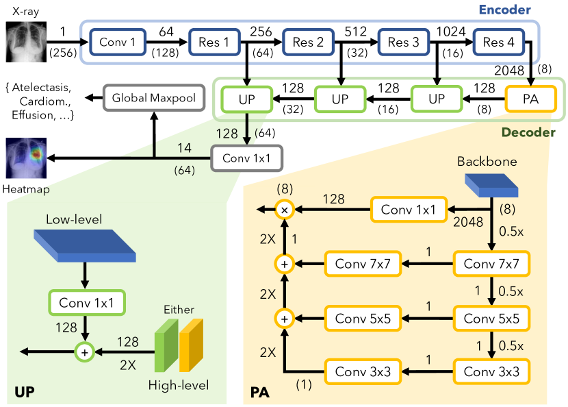
Fig. 1: Pyramid Localization Network (PYLON) with its Pyramid Attention (PA) and Upsampling (UP) modules. The model consists of two parts: an encoder and a decoder. The encoder could be ResNet, DenseNet or others. Here we assume the input of size $256\times 256$ and ResNet-50 as the encoder. Global Maxpool is used for image classification. Heatmap is the localization output. 2X refers to bilinear upsampling. 0.5X refers to max pooling. Each Conv is followed by a batch norm and a ReLU, except the Conv 1x1 before Global Maxpool which is not followed by any. The numbers denote the number of channels. The numbers in parentheses denote the size of the feature map.

1 Introduction

Class-Activation Map (CAM) [1, 2, 3] has been used for explaining a classification model’s decision by pointing to the region of high response for a specific class [4, 5, 6, 7]. In medical imaging, this helps clinicians quickly locate the region of interest and interpret the findings. Though CAM cannot provide precise boundaries of the region of interest, it can point localize with high accuracy. By pointing out the region of interest, CAM already provides an indispensable cue for radiologists and practitioners especially on small lesions, such as nodules, which are difficult to notice.

CAM, however, is not the only explainability method out there. Based on each method’s requirements, we can classify explainability methods into three categories: 1) requiring only input and output, e.g. SHAP [8] and LIME [9] 2) requiring the activations of some layers, e.g. CAM and its variants [1, 2, 3] 3) requiring the activations of all layers, e.g. [10, 11, 12]. Among these, CAM is the most popular for medical imaging due to its ease of use.

In chest x-ray for thorax diseases, the average size of abnormality in each class ranges from larger than $17\%$ (Cardiomegaly) to much smaller than $1\%$ (Nodule) of the total image area [7]. The size of the smallest class is so small, in fact, that it is even smaller than the resolution of a typical classification network’s last feature map. This clearly limits CAM’s ability to precisely localize objects in small classes.

CAM can be improved on four main fronts: 1) training schemes which include contrast-induced attention [13] and semi-supervised learning [6] 2) loss functions which include multi-instance learning [6] and its variant [14] 3) post-processing with CRF [14] and 4) architectures which include Blur pooling [15, 14] and high-resolution feature map [16]. We argue that the most straightforward way is to directly increase the feature map’s resolution which puts our work in the architecture category.

Usage of high resolution feature maps brings the design philosophy of our classification network closer to that of segmentation networks with large feature maps like [17, 18, 19]. Though related, these networks were designed for very different purposes under different assumptions. Naively applying CAM methods on segmentation models does not yield the good performance that one would expect. Our experiments suggest that Global Average Pooling (GAP) and Group Normalization [20] which are often utilized in segmentation networks should be avoided when adapting these models for a weakly-supervised localization task. To address this issue, we propose Pyramid Localization Network (PYLON), a model for high-accuracy weakly-supervised point localization. We demonstrated the localization accuracy on NIH’s Chest X-Ray 14 bounding-box annotated dataset [7].

2 Pyramid Localization Network

2.1 Naive implementation for higher resolution

In this subsection, we attempt to improve the localization performance of CAM by increasing the feature map’s resolution with segmentation models. A segmentation model consists of two parts: an encoder which could be ResNet [21], DenseNet [22] or others (usually known as backbones), and a decoder which is specific to each segmentation model. The two parts can be seen in Fig. 1. We consider three different decoder architectures, namely DeeplabV3+ [23], Feature Pyramid Network (FPN) [24, 25], and Pyramid Attention Network (PAN) [19], and a baseline model which contains only the encoder, which we call Backbone.

Class-activation map is obtained from the activations of the last feature map where each channel corresponds to a distinct class. 1x1 Conv is applied as needed to adjust the final number of channels to match the number of classes. Each channel is then globally max pooled to get a logit value for classification. The raw feature map before global pooling is output directly as the class-activation map (heatmap). Note that only image-level annotation is required to train the network. In our experiments, we used Chest X-Ray 14 dataset [7] as some of the images were annotated with bounding boxes that can be used for measuring the localization accuracy.

Results. We found CAMs produced by segmentation networks to be worse than those produced by the Backbone baseline in terms of localization despite having much higher resolution feature maps as seen in Table 2 and Fig. 2.

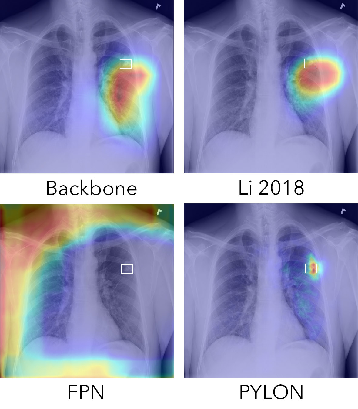
Fig. 2: Qualitative results for the class Nodule. Backbone and Li 2018 [6] produce low-resolution CAM. FPN produces unusable CAM highlighting only on the borders. PYLON (ours) produces highest localization accuracy. More qualitative results are available at https://github.com/cmb-chula/pylon.

2.2 Diagnosis and solution

In this subsection, we identify why segmentation models fail to produce accurate localization. The cause stems from the task mismatch. While segmentation models were designed for pixel-level annotation, only image-level annotation is available here, thereby making the task weakly-supervised. Without explicit guiding signal on the spatial information of the class object, this knowledge must be conveyed from the input image itself. This calls for a deep feature extractor with shift-equivariance property, i.e. a shifted input shifts the output by the same amount, that is able to preserve the spatial information from the input pixels through all the layers and present it on the corresponding locations of the output feature maps. Finally, these feature maps need to be transformed into class prediction. Without a proper care, the model may embed class information onto the spatial dimensions. A strategy to separate class information from spatial information is to generate one feature map for each class followed by global pooling for classification. This effectively preserves spatial information within each feature map and distributes class information along distinct feature maps. The combination of the two, shift-equivariant feature extractor and global pooling classifier produces a model with accurate class-activation maps.

The reason behind the high variance in localization accuracy of DeeplabV3+ (in Cardiomegaly) and PAN (overall) is that both networks utilize Global Average Pooling (GAP) in their decoders: in the Atrous Spatial Pyramid Pooling (ASPP) module in the case of DeeplabV3+, and in both the Feature Pyramid Attention (FPA) and the Global Attention Upsampling (GAU) modules in the case of PAN. It is clear that GAP destroys the localization information entirely, hence not shift equivariant. Even coupled with alternative paths, the localization accuracy takes a toll depending on the degree to which the GAP path is utilized. Some classes and some runs utilize the GAP path more than others resulting in poorer localization accuracy, and vice versa. To verify that this is the case, we removed all GAPs from both networks, and evaluate the changes in point localization accuracy (defined in section 3.2): DeeplabV3+’s accuracy increased from $0.35$ to $0.41$ due to lower variance in Cardiomegaly class, while PAN’s accuracy increased from $0.37$ to $0.57$ due to lower variance overall.

The failure of FPN [25] to localize (see Fig. 2) is another interesting case because there is no GAP in it. The problem is caused by group normalization layers [20] in its segmentation branch. The localization accuracy greatly improved from $0.08$ to $0.52$ by simply replacing group normalization with batch normalization [27]. This is unexpected because a group norm by itself should be shift equivariant. This suggests either a group norm coupled with other layers breaks this property, or there are more than one cause besides shift equivariancy. In any case, this opens up an opportunity for an interesting future work.

To summarize: Global Average Pooling and Group Normalization should not be used in models for weakly-supervised localization.

2.3 Pyramid Localization Network (PYLON)

With better understanding of what hinders localization accuracy, we design a new localization network by removing all global average pooling from PAN [19]. More specifically, we remove one in the Feature Pyramid Attention (FPA) module, and remove one in the Global Attention Upsampling (GAU) module. The new blocks are named PA and UP accordingly. Note that we propose to use 1x1 Conv in the UP module due to its superior localization ability. The new architecture is called Pyramid Localization Network (PYLON) and is depicted in Fig. 1 with detailed explanations. PYLON is simple in nature relying mostly on 1x1 Conv with little computation and memory overhead. The success of PYLON is to delegate work on its encoder which has seen continual developments [28].

Name	Atelectasis	Cardiom.	Effusion	Infiltration	Mass	Nodule	Pneumonia	Pneumoth.	Weighted avg.
$\mathbf{\mathbf{IoU}>0.25}$ or $\mathbf{\mathbf{IoR}>0.25}$
Backbone	$0.39\pm 0.02$	$1.0\pm 0.0$	$0.47\pm 0.04$	$0.67\pm 0.01$	$0.48\pm 0.02$	$0.01\pm 0.0$	$0.74\pm 0.02$	$0.17\pm 0.02$	$0.53\pm 0.01$
Li2018	$0.36\pm 0.02$	$0.99\pm 0.01$	$0.54\pm 0.02$	$0.73\pm 0.02$	$0.41\pm 0.05$	$0.04\pm 0.03$	$0.72\pm 0.04$	$\mathbf{0.23\pm 0.03}$	$0.54\pm 0.01$
PYLON (ours)	$\mathbf{0.63\pm 0.02}$	$1.0\pm 0.01$	$\mathbf{0.65\pm 0.01}$	$\mathbf{0.81\pm 0.03}$	$\mathbf{0.71\pm 0.04}$	$\mathbf{0.49\pm 0.05}$	$\mathbf{0.8\pm 0.03}$	$0.2\pm 0.02$	$\mathbf{0.68\pm 0.01}$
$\mathbf{\mathbf{IoU}>0.5}$ or $\mathbf{\mathbf{IoR}>0.5}$
Backbone	$0.17\pm 0.01$	$\mathbf{1.0\pm 0.0}$	$0.2\pm 0.03$	$0.36\pm 0.02$	$0.3\pm 0.02$	$0.0\pm 0.0$	$0.48\pm 0.04$	$0.12\pm 0.01$	$0.35\pm 0.01$
Li2018	$0.11\pm 0.01$	$0.97\pm 0.03$	$0.22\pm 0.01$	$0.44\pm 0.02$	$0.2\pm 0.03$	$0.0\pm 0.0$	$0.52\pm 0.05$	$0.13\pm 0.02$	$0.35\pm 0.01$
PYLON (ours)	$\mathbf{0.42\pm 0.03}$	$0.99\pm 0.01$	$\mathbf{0.48\pm 0.03}$	$\mathbf{0.59\pm 0.03}$	$\mathbf{0.61\pm 0.04}$	$\mathbf{0.35\pm 0.04}$	$\mathbf{0.7\pm 0.03}$	$\mathbf{0.15\pm 0.01}$	$\mathbf{0.55\pm 0.01}$

Table 1: Localization accuracy on Chest X-Ray 14 varying intersection thresholds.

Name	Atelectasis	Cardiom.	Effusion	Infiltration	Mass	Nodule	Pneumonia	Pneumoth.	Weighted avg.
Backbone	$0.32\pm 0.02$	$1.0\pm 0.0$	$0.3\pm 0.02$	$0.61\pm 0.03$	$0.4\pm 0.04$	$0.07\pm 0.01$	$0.56\pm 0.04$	$0.16\pm 0.01$	$0.45\pm 0.01$
Li2018	$0.32\pm 0.03$	$0.96\pm 0.04$	$0.5\pm 0.03$	$0.58\pm 0.02$	$0.44\pm 0.02$	$0.05\pm 0.02$	$0.59\pm 0.07$	$0.19\pm 0.04$	$0.48\pm 0.01$
DeeplabV3+∗	$0.18\pm 0.06$	$0.48\pm 0.44$	$0.34\pm 0.03$	$0.54\pm 0.07$	$0.52\pm 0.08$	$0.09\pm 0.01$	$0.47\pm 0.12$	$\mathbf{0.2\pm 0.01}$	$0.35\pm 0.07$
(No GAP)∗	$0.17\pm 0.06$	$0.92\pm 0.05$	$0.34\pm 0.1$	$0.53\pm 0.09$	$0.5\pm 0.1$	$0.08\pm 0.05$	$0.47\pm 0.1$	$0.18\pm 0.03$	$0.41\pm 0.01$
FPN	$0.06\pm 0.12$	$0.2\pm 0.45$	$0.11\pm 0.15$	$0.0\pm 0.0$	$0.06\pm 0.13$	$0.01\pm 0.01$	$0.1\pm 0.21$	$0.02\pm 0.04$	$0.08\pm 0.15$
(BN)	$0.42\pm 0.06$	$1.0\pm 0.0$	$0.4\pm 0.05$	$0.65\pm 0.04$	$0.56\pm 0.04$	$0.12\pm 0.05$	$0.68\pm 0.04$	$0.14\pm 0.01$	$0.52\pm 0.03$
PAN	$0.21\pm 0.23$	$0.63\pm 0.38$	$0.55\pm 0.1$	$0.27\pm 0.34$	$0.64\pm 0.04$	$0.02\pm 0.02$	$0.36\pm 0.31$	$0.16\pm 0.02$	$0.37\pm 0.18$
(No GAP)	$0.43\pm 0.05$	$0.99\pm 0.01$	$0.55\pm 0.01$	$0.67\pm 0.02$	$0.6\pm 0.04$	$0.33\pm 0.09$	$0.7\pm 0.03$	$0.14\pm 0.03$	$0.57\pm 0.02$
$\text{PYLON}_{\text{No PA}}$	$0.48\pm 0.03$	$0.98\pm 0.02$	$0.52\pm 0.04$	$0.67\pm 0.03$	$0.66\pm 0.02$	$\mathbf{0.48\pm 0.04}$	$0.7\pm 0.04$	$0.18\pm 0.01$	$0.6\pm 0.01$
$\text{PYLON}_{\text{ATT}}$	$0.5\pm 0.03$	$0.79\pm 0.44$	$\mathbf{0.57\pm 0.09}$	$0.65\pm 0.05$	$0.64\pm 0.03$	$0.39\pm 0.15$	$0.69\pm 0.04$	$0.16\pm 0.04$	$0.57\pm 0.09$
$\text{PYLON}_{\text{1UP}}$	$0.44\pm 0.1$	$0.99\pm 0.01$	$0.41\pm 0.08$	$0.67\pm 0.03$	$0.57\pm 0.05$	$0.14\pm 0.01$	$0.67\pm 0.04$	$0.16\pm 0.02$	$0.53\pm 0.03$
$\text{PYLON}_{\text{2UP}}$	$0.49\pm 0.03$	$1.0\pm 0.01$	$0.52\pm 0.05$	$0.68\pm 0.03$	$0.66\pm 0.02$	$0.41\pm 0.04$	$0.71\pm 0.03$	$0.17\pm 0.02$	$0.6\pm 0.01$
PYLON (ours)	$\mathbf{0.53\pm 0.03}$	$0.99\pm 0.01$	$0.56\pm 0.03$	$\mathbf{0.71\pm 0.03}$	$\mathbf{0.67\pm 0.04}$	$0.46\pm 0.03$	$\mathbf{0.72\pm 0.03}$	$0.18\pm 0.01$	$\mathbf{0.62\pm 0.01}$

Table 2: Point localization accuracy on Chest X-Ray 14. For segmentation networks i.e. DeeplabV3+, FPN, and PAN, we reported them as pairs with our proposed counterparts. ^∗DeeplabV3+ were run only 3 times due to high computation cost.

3 Experiments on Chest X-Ray

3.1 Dataset

Among large public chest x-ray datasets [7, 29, 30, 5], NIH’s Chest X-Ray 14 [7] is the only one that provides bounding-box level annotation. Chest X-Ray 14 comprises more than 100,000 frontal x-ray images among which lie almost 1,000 bounding box annotations across 880 images. This is used only for evaluating the quality of CAM. We used the reference train-test split, $86524:25596$. We further split the train part into train and validation sets, $78484:8040$. The validation set was used for model selection and learning rate reduction.

Note that the following variables affect the final performance. Split. We have found that random splits performed close to [4] and are much better than the official split used in our experiments. Image size. The size of the input image has a large effect on the localization accuracy. We resized the image (bicubic) to $256\times 256$ in all experiments.

3.2 Metric

There are no standard metrics for localization task. Thus, we report metrics used by several other works.

Localization accuracy. [6, 7] have proposed to use IoR, intersection over detected region, to quantify how much the predicted region intersects with the ground truth. The detected region is the binarization of the prediction after scaled to range of 0 to 1 without bounding box estimation. Following from [6], we used the binarization threshold of $0.5$. The localization accuracy is defined as the percentage of instances with either $\mathrm{IoR}>\tau$ or $\mathrm{IoU}>\tau$ where $\tau$ is some threshold, usually set to 0.1 [6] or 0.25 [7].

Point localization accuracy. This metric measures how often the model can pinpoint a location within a ground truth bounding box. It is defined as the percentage of instances where the pixel of the highest CAM value is within the ground truth bounding box. Similar metrics are used in [31, 10, 1]. We focus on this metric because it is invariant to thresholds.

Area Under ROC. AUROC has been used in previous works [4, 7, 5]. In this context, we aim to show that PYLON does not sacrifice the prediction prowess for interpretability.

3.3 Training details

Loss function. We used binary cross entropy with equal weights for multi-label classification. Optimizer. All models were trained with the batch size of 64 and Adam [32] with the learning rate of $10^{-4}$ and no weight decay. The learning rate is multiplied by 0.2 when the validation loss plateaus for more than a single epoch. The training stops when the learning rate reaches below $10^{-6}$. Backbone. All network encoders are ResNet-50 [21] pretrained on ImageNet. Augmentation. Random horizontal flip. Random resize crop from 0.7 to 1.0. Random rotation up to 90 degrees. Random brightness/contrast within $\pm 0.5$. Others. We ran each experiment with 5 different seeds and with Nvidia’s mixed-precision unless stated otherwise. We reported standard deviations as intervals.

3.4 Results

PYLON achieved highest localization accuracy. As baselines, we included our re-implementation results of Li 2018 [6] because it is well-known. We also included Backbone which is a plain ResNet-50 with max pooling which yields comparable results to CheXnet [4] and [7].

Under localization accuracy metric, shown in Table 1, we reported different thresholds, 0.25 and 0.5. PYLON came on top across all thresholds with larger gains on the stricter overlap thresholds. Under point localization accuracy metric, shown in Table 2, for most of the classes, PYLON outperformed other architectures by a large margin particularly in Nodule, which is the smallest and hence hardest of all. To allow fair comparison, we always bilinear interpolate the output of each network to match the input size, i.e. $256\times 256$.

PYLON does not sacrifice classification accuracy. We compared PYLON against Backbone, and found that both final macro average AUROCs are 0.82 and each class’ AUROC only differs within the margin of error.

3.5 Ablation studies

Each component in PYLON helps localization. The following experiments are to justify each component in PYLON: 1) $\text{PYLON}_{\text{No PA}}$; no PA module, replacing with 1x1 Conv, BN, ReLU instead, 2) $\text{PYLON}_{\text{ATT}}$; adding channel-wise attention in UP module like in GAU, The results in Table 2 support our design decisions, especially that of $\text{PYLON}_{\text{ATT}}$ whose high variance bolsters our intuition about GAP even if it is used in channel-wise attention which is not the main path.

Higher resolution feature maps help localization. This could be answered by reducing the number of UP modules from the original three to two and one, $\text{PYLON}_{\text{2UP}}$, $\text{PYLON}_{\text{1UP}}$. Following from Table 2, we see large improvement from $\text{1UP}\rightarrow\text{2UP}$, less so from $\text{2UP}\rightarrow\text{3UP}$, with Nodule being the most improved from higher resolution.

4 Conclusion

We identified that shift-equivariance is important for accurate weakly-supervised localization. This suggests avoiding Global Average Pooling in the model. Quite surprisingly, we also found that Group normalization hinders localization with a reason yet to be determined. With this knowledge, we designed PYLON which produces high resolution yet accurate CAM. It performed strongly in weakly-supervised localization task on Chest X-Ray 14 dataset across multiple metrics while not sacrificing prediction accuracy.

References

- [1] M Oquab, L Bottou, I Laptev, et al., “Is object localization for free? - weakly-supervised learning with convolutional neural networks,” in 2015 IEEE Conference on Computer Vision and Pattern Recognition (CVPR), June 2015, pp. 685–694.
- [2] B Zhou, A Khosla, A Lapedriza, et al., “Learning deep features for discriminative localization,” in 2016 IEEE Conference on Computer Vision and Pattern Recognition (CVPR), June 2016, pp. 2921–2929.
- [3] R R Selvaraju, M Cogswell, A Das, et al., “Grad-CAM: Visual explanations from deep networks via Gradient-Based localization,” in 2017 IEEE International Conference on Computer Vision (ICCV), Oct. 2017, pp. 618–626.
- [4] Pranav Rajpurkar, Jeremy Irvin, Kaylie Zhu, et al., “CheXNet: Radiologist-Level pneumonia detection on chest X-Rays with deep learning,” pp. 3–9, Nov. 2017.
- [5] Jeremy Irvin, Pranav Rajpurkar, Michael Ko, et al., “CheXpert: A large chest radiograph dataset with uncertainty labels and expert comparison,” AAAI, vol. 33, pp. 590–597, July 2019.
- [6] Z Li, C Wang, M Han, et al., “Thoracic disease identification and localization with limited supervision,” in 2018 IEEE/CVF Conference on Computer Vision and Pattern Recognition, June 2018, pp. 8290–8299.
- [7] X Wang, Y Peng, L Lu, et al., “ChestX-Ray8: Hospital-Scale chest X-Ray database and benchmarks on Weakly-Supervised classification and localization of common thorax diseases,” in 2017 IEEE Conference on Computer Vision and Pattern Recognition (CVPR), July 2017, pp. 3462–3471.
- [8] Scott M Lundberg and Su-In Lee, “A unified approach to interpreting model predictions,” in Advances in Neural Information Processing Systems 30 (NIPS 2017), I Guyon, U V Luxburg, S Bengio, et al., Eds. 2017, pp. 4765–4774, Curran Associates, Inc.
- [9] Marco Tulio Ribeiro, Sameer Singh, and Carlos Guestrin, ““why should I trust you?”: Explaining the predictions of any classifier,” in Proceedings of the 22nd ACM SIGKDD International Conference on Knowledge Discovery and Data Mining, New York, NY, USA, Aug. 2016, KDD ’16, pp. 1135–1144, Association for Computing Machinery.
- [10] Jianming Zhang, Sarah Adel Bargal, Zhe Lin, et al., “Top-Down neural attention by excitation backprop,” Int. J. Comput. Vis., vol. 126, no. 10, pp. 1084–1102, Oct. 2018.
- [11] Avanti Shrikumar, Peyton Greenside, and Anshul Kundaje, “Learning important features through propagating activation differences,” in Proceedings of the 34th International Conference on Machine Learning - Volume 70. Aug. 2017, ICML’17, pp. 3145–3153, JMLR.org.
- [12] Sebastian Bach, Alexander Binder, Grégoire Montavon, et al., “On Pixel-Wise explanations for Non-Linear classifier decisions by Layer-Wise relevance propagation,” PLoS One, vol. 10, no. 7, pp. e0130140, July 2015.
- [13] J Liu, G Zhao, Y Fei, et al., “Align, attend and locate: Chest X-Ray diagnosis via contrast induced attention network with limited supervision,” in 2019 IEEE/CVF International Conference on Computer Vision (ICCV), Oct. 2019, pp. 10631–10640.
- [14] Eyal Rozenberg, Daniel Freedman, and Alex Bronstein, “Localization with limited annotation for chest x-rays,” in Proceedings of the Machine Learning for Health NeurIPS Workshop 2019, Adrian V Dalca, Matthew B A McDermott, Emily Alsentzer, et al., Eds. 2020, vol. 116 of Proceedings of Machine Learning Research, pp. 52–65, PMLR.
- [15] Richard Zhang, “Making convolutional networks Shift-Invariant again,” in Proceedings of the 36th International Conference on Machine Learning, PMLR, Apr. 2019.
- [16] Li Yao, Jordan Prosky, Eric Poblenz, et al., “Weakly supervised medical diagnosis and localization from multiple resolutions,” Mar. 2018.
- [17] Olaf Ronneberger, Philipp Fischer, and Thomas Brox, “U-Net: Convolutional networks for biomedical image segmentation,” in Medical Image Computing and Computer-Assisted Intervention – MICCAI 2015. 2015, pp. 234–241, Springer International Publishing.
- [18] Liang-Chieh Chen, George Papandreou, Florian Schroff, et al., “Rethinking atrous convolution for semantic image segmentation,” June 2017.
- [19] Hanchao Li, Pengfei Xiong, Jie An, et al., “Pyramid attention network for semantic segmentation (BMVC 2018),” in 29th British Machine Vision Conference (BMVC 2018), May 2018.
- [20] Yuxin Wu and Kaiming He, “Group normalization,” in Computer Vision – ECCV 2018. 2018, pp. 3–19, Springer International Publishing.
- [21] K He, X Zhang, S Ren, et al., “Deep residual learning for image recognition,” in 2016 IEEE Conference on Computer Vision and Pattern Recognition (CVPR), June 2016, pp. 770–778.
- [22] Carl F Sabottke and Bradley M Spieler, “The effect of image resolution on deep learning in radiography,” Radiology: Artificial Intelligence, vol. 2, no. 1, pp. e190015, Jan. 2020.
- [23] Liang-Chieh Chen, Yukun Zhu, George Papandreou, et al., “Encoder-Decoder with atrous separable convolution for semantic image segmentation,” in Computer Vision – ECCV 2018. 2018, pp. 833–851, Springer International Publishing.
- [24] Alexander Kirillov, Kaiming He, Ross Girshick, et al., “A unified architecture for instance and semantic segmentation,” 2019.
- [25] Alexander Kirillov, Ross Girshick, Kaiming He, et al., “Panoptic feature pyramid networks,” in 2019 IEEE/CVF Conference on Computer Vision and Pattern Recognition (CVPR). June 2019, pp. 6392–6401, IEEE.
- [26] Pavel Yakubovskiy, “Segmentation models pytorch,” https://github.com/qubvel/segmentation_models.pytorch, 2020.
- [27] Sergey Ioffe and Christian Szegedy, “Batch normalization: Accelerating deep network training by reducing internal covariate shift,” in Proceedings of the 32nd International Conference on Machine Learning (ICML 2015). July 2015, ICML’15, pp. 448–456, JMLR.org.
- [28] Mingxing Tan and Quoc Le, “EfficientNet: Rethinking model scaling for convolutional neural networks,” in Proceedings of the 36th International Conference on Machine Learning, PMLR, Kamalika Chaudhuri and Ruslan Salakhutdinov, Eds., Long Beach, California, USA, 2019, vol. 97 of Proceedings of Machine Learning Research, pp. 6105–6114, PMLR.
- [29] Aurelia Bustos, Antonio Pertusa, Jose-Maria Salinas, et al., “PadChest: A large chest x-ray image dataset with multi-label annotated reports,” Med. Image Anal., vol. 66, pp. 101797, Aug. 2020.
- [30] Alistair E W Johnson, Tom J Pollard, Nathaniel R Greenbaum, et al., “MIMIC-CXR-JPG, a large publicly available database of labeled chest radiographs,” Jan. 2019.
- [31] Y Zhu, Y Zhou, Q Ye, et al., “Soft proposal networks for weakly supervised object localization,” in 2017 IEEE International Conference on Computer Vision (ICCV), Oct. 2017, pp. 1859–1868.
- [32] Diederik P Kingma and Jimmy Ba, “Adam: A method for stochastic optimization,” in 3rd International Conference on Learning Representations, ICLR 2015, 2015.