Supplementary Materials for “High-efficiency arbitrary quantum operation on a high-dimensional quantum system”

I Experimental Device and Setup

Our experimental system consists of a superconducting transmon qubit dispersively coupled to two rectangular microwave cavities, which are machined with high purity 5N5 aluminum. The transmon qubit is used as the ancilla, fabricated on a sapphire substrate with an energy relaxation time of $30~{}\mathrm{\mu s}$ and a pure dephasing time of $120~{}\mathrm{\mu s}$. The storage cavity has a single-photon lifetime of $143\,\mathrm{\mu s}$ with its lowest four Fock levels being employed as the qudit with a dimension of $d=4$. The ancilla qubit can be read out with a high fidelity through another cavity with a lifetime of 44 ns. The detailed geometry of the device and measurement setup can be found in our previous work Hu et al. (2019).

The system Hamiltonian is given by

$$H/\hbar=\omega_{\mathrm{s}}a^{\dagger}a+\omega_{\mathrm{a}}\left|e\right\rangle\left\langle e\right|-\chi_{\mathrm{s}}a^{\dagger}a\left|e\right\rangle\left\langle e\right|,$$ (S1)

where $a$ and $a^{\dagger}$ are the ladder operators of the storage cavity with a mode frequency $\omega_{s}/2\pi=7.634~{}\mathrm{GHz}$, $\omega_{a}/2\pi=5.692~{}\mathrm{GHz}$ is the transition frequency of the transmon between the ground state $\left|g\right\rangle$ and the excited state $\left|e\right\rangle$, and $\chi_{s}/2\pi=1.90~{}\mathrm{MHz}$ is the dispersive coupling strength between the transmon and the storage cavity.

The general architecture and scheme for realizing the arbitrary quantum operation (AQuO) are illustrated in Fig. 1 in the main text. The AQuO can be realized in three steps: (i) a unitary gate on the composite of the quantum system and the ancilla, (ii) the readout of the ancilla, and (iii) the reset of the ancilla.

Step (i) corresponds to a universal control of the closed composite of the quantum system and the ancilla. According to the nonlinear interaction Eq. (S1), an arbitrary unitary gate could be realized by using selective number-dependent arbitrary phase gates (SNAP) Krastanov et al. (2015); Heeres et al. (2017) on the ancilla in combination with displacement gates on the cavity. In this work, we instead use the gradient ascent pulse engineering (GRAPE) method Khaneja et al. (2005); De Fouquieres et al. (2011) to numerically optimize the control pulses based on carefully calibrated experimental parameters to realize the unitary gates. We note that the GRAPE pulse length is mainly limited by the dispersive coupling strength $\chi_{s}$, and for a moderate $d\leq 5$, the pulse length is pretty independent of the number $d$ of the Fock levels that are employed. However, when $d$ gets even larger, the higher-order terms of the cavity-transmon interaction and decoherence effects will start to matter, demanding higher control precision and longer pulse length. The control microwave drives are generated by field-programmable gate arrays (FPGAs) based on all previously recorded ancilla measurement outcomes in the classical register. The fast real-time adaptive control is the key technology for AQuO and is also realized with the FPGAs with home-made logics.

For step (ii), the quantum state of the ancilla qubit is read out with the assistance of a readout cavity mode and a Josephson parametric amplifier Hatridge et al. (2011); Murch et al. (2013). The readout results are requisite, registered, and processed by the FPGAs. With our current experimental apparatus, the readout fidelities are $>$99.9% for $\left|g\right\rangle$ and 98.9% for $\left|e\right\rangle$ of the ancilla qubit with a measurement time of $320~{}\mathrm{ns}$.

In step (iii), to reset the ancilla qubit requires no effect on the photonic system during the resetting process. In our experiment, we use the measurement-based adaptive control to reset the ancilla qubit by applying a $\pi$-pulse conditional on the measurement outcome $\left|e\right\rangle$ of the ancilla.

In addition to the realization of AQuOs with the circuit in Fig. 1 in the main text, we also need to characterize the performance of AQuOs by process tomography Nielsen and Chuang (2000). The process tomography of the AQuOs is realized with the assistance of the ancilla by preparing the qudit into a set of linearly independent basis states and performing the state tomography on the output of the AQuOs. The initialization and measurement of the qudit are achieved via the encoding and decoding gates based on the universal control of the composite photonic qudit-ancilla system via the GRAPE method. For example, the encoding and decoding gates for the odd-parity subspace stabilization are

$$\begin{split}\left|0\right\rangle\left|g\right\rangle\to\left|1\right\rangle\left|g\right\rangle,\\ \left|0\right\rangle\left|e\right\rangle\to\left|3\right\rangle\left|g\right\rangle,\end{split}$$ (S2)

and

$$\begin{split}\left|1\right\rangle\left|g\right\rangle\to\left|0\right\rangle\left|g\right\rangle,\\ \left|3\right\rangle\left|g\right\rangle\to\left|0\right\rangle\left|e\right\rangle,\end{split}$$ (S3)

respectively.

II Basics about quantum operations

II.1 Kraus operators

The open quantum system dynamics has many representations, such as superoperators in Liouville space, Kraus operators, Choi matrix, and system-environment representations Gilchrist et al. (2005); Nielsen and Chuang (2000). The Kraus representation of a quantum operation can be written as Nielsen and Chuang (2000)

$$\rho_{s}\mapsto\mathcal{E}\left(\rho_{s}\right)=\sum_{j=0}^{l-1}E_{j}\rho_{s}E_{j}^{\dagger},$$ (S4)

where $1\leq l\leq d^{2}$ ($d$ is the Hilbert space dimension), $\rho_{s}$ is the density matrix of the quantum system, and the Kraus operators satisfy

$$\sum_{j=0}^{l-1}E_{j}^{\dagger}E_{j}=\mathbf{I},$$ (S5)

where $\mathbf{I}$ is the unity matrix.

Without being limited by the experimental resources, the conventional approach to realize an AQuO on a $d$-dimensional quantum system is to introduce an extra ancillary system serving as the environment to dilate the whole Hilbert space. A unitary gate on the composite quantum system-ancilla is then implemented followed by the ancilla reset. For an ancilla with a dimension of $l$, the unitary gate is given by

$$U=\begin{pmatrix}E_{0}&*&...&*\\ E_{1}&*&...&*\\ ...&*&...&*\\ E_{l-1}&*&...&*\end{pmatrix},$$ (S6)

with the dimension of the whole system being $d\times l$. Here, ‘*’ means the specific matrix element is trivial because it will not affect the target quantum system. We then have:

$$U\left[\left|0\right\rangle\left\langle 0\right|\otimes\rho_{s}\right]U^{\dagger}=\Sigma_{j_{1}j_{2}}\left|j_{1}\right\rangle\left\langle j_{2}\right|\otimes E_{j_{1}}\rho_{s}E_{j_{2}}^{\dagger}.$$ (S7)

Here, $E_{j}$ is the Kraus operator with a dimension of $d$, the subscript $j$ denotes the outcome of the ancilla in its orthonormal basis $\left|j\right\rangle$ ($j\in\left\{0,...,l-1\right\}$) after implementing the unitary gate $U$, and the initial state of the ancilla is $\left|0\right\rangle$. Tracing out the ancilla, one gets the quantum operation

$$\mathcal{E}(\rho_{s})=\Sigma_{j=0}^{l-1}E_{j}\rho_{s}E_{j}^{\dagger}.$$ (S8)

Note that the quantum operation is invariant with respect to the choice of the ancilla basis. Therefore, for an arbitrary ancilla basis $\left|\tilde{\psi}_{k}\right\rangle=\sum_{j=0}^{l-1}u_{kj}^{*}\left|j\right\rangle$ with an $\tilde{l}\times\tilde{l}$ unitary transformation $\boldsymbol{u}$ with a dimension $\tilde{l}\geq l$, we have the corresponding Kraus operator representation as

$$\mathrm{Tr}\left[U\left|0\right\rangle\left\langle 0\right|\otimes\rho_{\mathrm{s}}U^{\dagger}\right]$$

$$=\sum_{k=0}^{\tilde{l}-1}\left\langle\tilde{\psi}_{k}\right|\Sigma_{j_{1}j_{2}}\left|j_{1}\right\rangle\left\langle j_{2}\right|\otimes E_{j_{1}}\rho_{\mathrm{s}}E_{j_{2}}^{\dagger}\left|\tilde{\psi}_{k}\right\rangle$$

$$=\sum_{k=0}^{\tilde{l}-1}\left[\sum_{j_{1}}\langle\tilde{\psi}_{k}\left|j_{1}\right\rangle E_{j_{1}}\right]\rho_{\mathrm{s}}\left\{\left[\sum_{j_{2}}\langle\tilde{\psi}_{k}\left|j_{2}\right\rangle E_{j_{2}}\right]\right\}^{\dagger}$$

$$=\sum_{k=0}^{\tilde{l}-1}F_{k}\rho_{s}F_{k}^{\dagger},$$ (S9)

with $F_{k}=\sum_{j}u_{kj}E_{j}$.

This indicates that both the Kraus representation of an operation and the approach to realize a given quantum operation are not unique. The Kraus rank of an operation ($m$) is the number of the irreducible Kraus operator elements, which satisfies $1\leq m\leq d^{2}$. Therefore, for AQuOs this conventional method needs an ancilla with a dimension of $d^{2}$ and an arbitrary unitary gate on a $d^{3}$-dimensional Hilbert space.

II.2 Master equation

It is well-known that the continuous evolution of an open quantum system follows the master equation, in the Lindblad form as Pet ; Gardiner and Zoller (2004)

$$\frac{d}{dt}\rho_{s}\left(t\right) =\sum_{j=0}^{l-2}\kappa_{j}\left(2o_{j}\rho_{s}\left(t\right)o_{j}^{\dagger}-o_{j}^{\dagger}o_{j}\rho_{s}\left(t\right)-\rho_{s}\left(t\right)o_{j}^{\dagger}o_{j}\right).$$ (S10)

Here, $\kappa_{j}$ and $o_{j}$ are the rate and the operator for the $j$-th decoherence process, respectively. To mimic an arbitrary decoherence process of a quantum system, we could construct $l-1$ independent environments $\sum_{\omega}b_{j}\left(\omega\right)$, with $b_{j}\left(\omega\right)$ denoting the bosonic operator for a continuum mode at a frequency $\omega$ of the $j$-th environment, and realize the system-environment coupling Hamiltonian $H_{j}=\sum_{\omega}\left[g_{j}\left(\omega\right)b_{j}\left(\omega\right)o_{j}^{\dagger}+g_{j}^{*}(\omega)b_{j}^{\dagger}\left(\omega\right)o_{j}\right]$. For a Markovian environment, $g_{j}\left(\omega\right)\approx g_{j}$ is independent of $\omega$ and we could derive the Lindblad form of the master equation by tracing over the environments, and the corresponding decoherence rates $\kappa_{j}=g_{j}^{2}\rho_{j}$ with $\rho_{j}$ denoting the density of the continuum states for the $j$-th environment. Therefore, such an analog approach to realize the open quantum system evolution is resource demanding because of the challenges in the construction of Markovian environments and arbitrary system-environment interaction Hamiltonians.

II.3 Master equation to AQuO conversion

From another perspective, by discretizing the evolution into steps with $dt\rightarrow 0$, we have the dynamics of the open quantum system as

$$\rho_{s}\left(t+dt\right)= \rho_{s}\left(t\right)+\sum_{j=0}^{{l-2}}\mathcal{L}_{j}\left(\rho_{s}\right)dt$$

$$+\mathcal{O}\left[\sum_{j=0}^{{l-2}}\left(\kappa_{j}dt\right)^{2}\rho_{s}\left(t\right)\right].$$ (S11)

with Liouvillian $\mathcal{L}_{j}$ describing the incoherent evolution. Introducing the Kraus operators

$$E_{j} =\sqrt{2\kappa_{j}dt}o_{j},~{}\mathrm{for}~{}j\in\left[0,l-2\right]$$ (S12)

$$E_{l-1} =\mathbf{I}-\sum_{j=0}^{l-2}\kappa_{j}dto_{j}^{\dagger}o_{j},$$ (S13)

we have an equivalent operation on the system as

$$\rho_{s}\left(t+dt\right)=\mathcal{E}\left(\rho_{s}\left(t\right)\right)=\sum_{j=0}^{{l-1}}E_{j}\rho_{s}\left(t\right)E_{j}^{\dagger}+\mathcal{O}\left[\left(\kappa dt\right)^{2}\rho_{s}\left(t\right)\right].$$ (S14)

Therefore, the master equation evolution could be approximated by a repetitive implementation of Kraus operators with $\kappa dt\ll 1$.

II.4 Quantum trajectory simulation

The evolution of an open quantum system, i.e. the above derived master equation, could also be interpreted as a quantum jump process: the quantum system changes the environment state from $\left|0\right\rangle$ to $\left|j\right\rangle$ randomly and instantly. Therefore, the dynamics of the system follows a stochastic process

$$\rho_{s}\left(t+dt\right)\mapsto\frac{E_{j}\rho_{s}\left(t\right)E_{j}^{\dagger}}{p_{j}},$$ (S15)

with the jump probability of

$$p_{j}=\mathrm{Tr}\left[E_{j}\rho_{s}\left(t\right)E_{j}^{\dagger}\right].$$ (S16)

In numerical simulations, we can implement the quantum trajectory simulation by estimating $\left\{p_{j}\right\}$ and generating a random number $r\in\left[0,1\right]$, followed by choosing the $j$-th jump if $\sum_{i=0}^{j-1}p_{i}\leq r<\sum_{i=0}^{j}p_{i}$. In experiments, the AQuOs applied to the quantum system could be treated as generalized measurements by the ancilla, and the system randomly jumps and evolves conditional on the ancilla outcome $j$. When characterizing the system states, we repetitively perform the trajectories and thus obtain the results of unconditioned open system dynamics by averaging over many different trajectories. As indicated by Eq. (S9), the choice of the quantum jump operators to realize a quantum trajectory is not unique, and this property of the quantum trajectory simulation is known as unravelling Wiseman and Doherty (2005).

II.5 Quantum measurement

For a general measurement process, the ancilla interacts with the quantum system through a unitary gate that has a similar form as the environment-system interaction. According to Eq. (S7), the output of the ancilla reads

$$\mathrm{Tr}_{\mathrm{system}}\left\{U\left[\left|0\right\rangle\left\langle 0\right|\otimes\rho_{s}\right]U^{\dagger}\right\}$$

$$=\Sigma_{j_{1}j_{2}}\left|j_{1}\right\rangle\left\langle j_{2}\right|\otimes\mathrm{Tr}\left(E_{j_{1}}\rho_{s}E_{j_{2}}^{\dagger}\right).$$ (S17)

Therefore, for the ancilla measurement outcome of $\left|j\right\rangle$, we have the probability of

$$p_{j} =\left\langle j\right|\mathrm{Tr}_{\mathrm{system}}\left\{U\left[\left|0\right\rangle\left\langle 0\right|\otimes\rho_{s}\right]U^{\dagger}\right\}\left|j\right\rangle$$

$$=\mathrm{Tr}\left(E_{j}\rho_{s}E_{j}^{\dagger}\right)$$

$$=\mathrm{Tr}\left(M_{j}\rho_{s}\right),$$ (S18)

with a positive operator valued measure (POVM) $M_{j}=E_{j}^{\dagger}E_{j}$. Therefore, with the same setup for the AQuO, we can perform arbitrary POVMs on a qudit by recording the ancilla measurement output. As shown in Fig. 3 in the main text, the circuit to realize AQuOs is equivalent to a binary-tree structure. Therefore, the realization of POVMs by AQuO is equivalent to the binary search trees for generalized measurements proposed by Andersson and Oi Andersson and Oi (2008).

II.6 Process matrix

Representing the Kraus operators in a certain basis, the quantum operations can also be expressed by the process ($\chi$) matrix Gilchrist et al. (2005); Bhandari and Peters (2016)

$$\rho_{s}\rightarrow\sum_{m,n}\chi_{mn}\widetilde{E_{m}}\rho_{s}\widetilde{E_{n}}^{\dagger}.$$ (S19)

Here, for a $d$-dimensional system, the $\chi$ matrix contains $d^{4}-d^{2}$ independent parameters under the constraints $\sum_{m,n}\chi_{mn}\widetilde{E_{n}}^{\dagger}\widetilde{E_{m}}=\mathbf{I}$. When characterizing the $\chi$ matrix, we prepare a set of complete input states for each operation which are linearly independent in the density matrix representation. Then, we reconstruct $\chi$ matrix by tomography of the output states and represent it with a set of complete orthogonal operators.

For a qubit ($d=2$), we choose Pauli matrices as the operation basis. For $d=4$, we choose 16 operators that correspond to the tensor product of two Pauli operators by decomposing the system into two qubits. For $d=3$, we choose complete orthogonal operators Gell-Mann matrices $\{\Lambda_{i}\}$:

$$\Lambda_{1}=\begin{pmatrix}1&0&0\\ 0&1&0\\ 0&0&1\end{pmatrix}, \quad\Lambda_{2}=\sqrt{3/2}\begin{pmatrix}0&1&0\\ 1&0&0\\ 0&0&0\end{pmatrix},$$

$$\Lambda_{3}=\sqrt{3/2}\begin{pmatrix}0&-1&0\\ 1&0&0\\ 0&0&0\end{pmatrix}, \quad\Lambda_{4}=\sqrt{3/2}\begin{pmatrix}1&0&0\\ 0&-1&0\\ 0&0&0\end{pmatrix},$$

$$\Lambda_{5}=\sqrt{3/2}\begin{pmatrix}0&0&1\\ 0&0&0\\ 1&0&0\end{pmatrix}, \quad\Lambda_{6}=\sqrt{3/2}\begin{pmatrix}0&0&-1\\ 0&0&0\\ 1&0&0\end{pmatrix},$$

$$\Lambda_{7}=\sqrt{3/2}\begin{pmatrix}0&0&0\\ 0&0&1\\ 0&1&0\end{pmatrix}, \quad\Lambda_{8}=\sqrt{3/2}\begin{pmatrix}0&0&0\\ 0&0&-1\\ 0&1&0\end{pmatrix},$$

$$\Lambda_{9}=\sqrt{1/2}\begin{pmatrix}1&0&0\\ 0&1&0\\ 0&0&-2\end{pmatrix},$$

where the coefficient in each operator ensures the same inner product $\mathrm{Tr}(\Lambda_{i}^{\dagger}\Lambda_{i})=3$.

III Experimental construction of AQuOs

For a given target quantum operation, generally in the Kraus operator representation, we convert it to the system-environment representation and realize it using the quantum circuit that is shown in Fig. 1 in the main text.

For a rank-2 AQuO, since the ancilla has a dimension of two, we can directly construct the unitary gate that satisfies

$$U\left[\left|g\right\rangle\left\langle g\right|\otimes\rho_{s}\right]U^{\dagger}$$

$$= \left|g\right\rangle\left\langle g\right|\otimes E_{0}\rho_{s}E_{0}^{\dagger}+\left|e\right\rangle\left\langle e\right|\otimes E_{1}\rho_{s}E_{1}^{\dagger}$$

$$+\left|g\right\rangle\left\langle e\right|\otimes E_{0}\rho_{s}E_{1}^{\dagger}+\left|e\right\rangle\left\langle g\right|\otimes E_{1}\rho_{s}E_{0}^{\dagger}.$$ (S20)

As described in the previous sections, the AQuOs require universal control of the composite system-ancilla. We use the GRAPE method in our experiments to numerically optimize the drive pulses for the desired unitary gates with the device parameters that are all experimentally calibrated. For the optimization, a set of arbitrary and completely independent states have been chosen, and the control pulses are optimized to achieve the highest average fidelity of the output states compared with the expected ones from the target unitary gates. Since the unitary gates on the qudit with $d=4$ in our experiment only affect the first four Fock levels of the storage cavity mode, four completely independent states which are superpositions of the first four levels of the system in combination with the ground state of the ancilla are enough to constrain the target unitary. More states (over complete) for the constraints lead to a higher precision of the optimized control pulses, but cost more time in the optimization.

For AQuOs with higher ranks, we first decompose the AQuOs into a sequence of rank-2 AQuOs. All the rank-2 AQuOs could be constructed following the procedure described above. In the follows, we provide more details of the schemes presented in the main text.

III.1 Odd-parity stabilization

To stabilize the Hilbert space spanned by Fock states of odd parity, i.e. $\left\{\left|1\right\rangle,\,\left|3\right\rangle\right\}$ of the photonic qudit ($d=4$), we have engineered the quantum operation with two Kraus operators

$$E_{0}=\begin{pmatrix}0&0&0&0\\ 0&1&0&0\\ 0&0&0&0\\ 0&0&0&1\end{pmatrix},\quad E_{1}=\begin{pmatrix}0&0&0&0\\ 1&0&0&0\\ 0&0&0&0\\ 0&0&1&0\end{pmatrix}.$$ (S21)

We note that under these operators, any state in the odd-parity subspace $\mathrm{span}\left\{\left|1\right\rangle,\,\left|3\right\rangle\right\}$ is conserved. In contrast, any state outside the odd-parity subspace will be mapped into the odd-parity subspace.

It is also worth noting that a state satisfying $E_{1}\left|\psi_{D}\right\rangle=0$ would be a dark state that remains invariant under these operators. For instance, $\tilde{E}_{1}=\left|1\right\rangle\left\langle 0\right|+\left|1\right\rangle\left\langle 2\right|$ could map states back to the odd-parity subspace, however, there is a dark state $\frac{1}{\sqrt{2}}\left(\left|0\right\rangle-\left|2\right\rangle\right)$ outside the odd-parity subspace that could not be stabilized. Our choice of the Kraus operators has a matrix rank of two that avoids the dark states outside the odd-parity subspace.

III.2 Two-photon dissipation

To realize quantum Zeno blockade, we need a two-photon dissipation operation which converts populations from Fock energy levels $\left|3\right\rangle\rightarrow\left|1\right\rangle$ and $\left|2\right\rangle\rightarrow\left|0\right\rangle$ by eliminating two photons simultaneously. Conventionally, the two-photon dissipation has been applied in various experiments to allow the stabilization of non-classical states Touzard et al. (2018) and realize quantum gates between bosonic modes Franson et al. (2004). For the continuous variable case, the master equation of the two-photon dissipation process is

$$\frac{d}{dt}\rho_{s}=\frac{\kappa}{2}\left[2a^{2}\rho_{s}\left(a^{\dagger}\right)^{2}-\left(a^{\dagger}\right)^{2}a^{2}\rho_{s}-\rho_{s}\left(a^{\dagger}\right)^{2}a^{2}\right],$$ (S22)

with $\kappa$ being the decay rate. In a truncated space ($d=4$), we can approximate the process as

$$\frac{d}{dt}\rho_{s}=\frac{\kappa}{2}\left[2o\rho_{s}o^{\dagger}-o^{\dagger}o\rho_{s}-\rho_{s}o^{\dagger}o\right],$$ (S23)

with $o=\sqrt{2}\left|0\right\rangle\left\langle 2\right|+\sqrt{6}\left|1\right\rangle\left\langle 3\right|$. For $dt\rightarrow 0$, according to Eq. (S11), the equivalent Kraus operator representation is $E_{0}=\mathbf{I}-\frac{\kappa dt}{2}o^{\dagger}o$ and $E_{1}=\sqrt{\kappa dt}o$. For practical experiments, the AQuOs are implemented with a finite repetitive duration $t_{\mathrm{int}}$, thus we approximate the two-photon dissipation process through two Kraus operators

$$E_{0} =\begin{pmatrix}1&0&0&0\\ 0&1&0&0\\ 0&0&e^{-\kappa t_{{\rm{int}}}}&0\\ 0&0&0&e^{-3\kappa t_{{\rm{int}}}}\end{pmatrix},$$ (S24)

$$E_{1} =\begin{pmatrix}0&0&\sqrt{1-e^{-2\kappa t_{{\rm{int}}}}}&0\\ 0&0&0&\sqrt{1-e^{-6\kappa t_{{\rm{int}}}}}\\ 0&0&0&0\\ 0&0&0&0\end{pmatrix}.$$ (S25)

Here, $\kappa t_{{\rm{int}}}$ is the two-photon dissipation parameter for each implementation of the operation. For the simulation of quantum trajectory, the operation is implemented repetitively with an interval of $t_{{\rm{int}}}$, leading to an effective two-photon dissipation rate of $\kappa$.

III.3 AQuOs with arbitrary rank

In this section we will show a general method to construct an arbitrary quantum channel with arbitrary ranks of Kraus operators. As proposed by Shen $et~{}al$. Shen et al. (2017) and also schematically illustrated in Fig. 3 in the main text, an AQuO with an arbitrary rank could be realized by $n$-step adaptive implementations of the elementary rank-2 AQuOs (a binary tree with $n$ layers). Here, we take the full-rank AQuO ($\left\{E_{k}\right\}$, $k=0,...,15$) for a photonic qudit with $d=4$ as an example, which is illustrated in Fig. 3 in the main text.

(1) The first step is to decompose the AQuO into Kraus operators at each layer and construct the binary tree for the target AQuO. The first layer realizes the rank-2 AQuO:

$$A_{0}^{\dagger}A_{0} =E_{0}^{\dagger}E_{0}+...+E_{7}^{\dagger}E_{7},$$ (S26)

$$A_{1}^{\dagger}A_{1} =E_{8}^{\dagger}E_{8}+...+E_{15}^{\dagger}E_{15}.$$ (S27)

Therefore, we have

$$A_{0} =\sqrt{E_{0}^{\dagger}E_{0}+...+E_{7}^{\dagger}E_{7}},$$ (S28)

$$A_{1} =\sqrt{E_{8}^{\dagger}E_{8}+...+E_{15}^{\dagger}E_{15}}.$$ (S29)

Depending on the ancilla measurement output $\{0,1\}$, corresponding to the subscript of $A$, in the first layer, for example, we have

$$\left(B_{00}A_{0}\right)^{\dagger}\left(B_{00}A_{0}\right)=E_{0}^{\dagger}E_{0}+...+E_{3}^{\dagger}E_{3},$$ (S30)

and thus the second layer realizes

$$B_{00} =\sqrt{E_{0}^{\dagger}E_{0}+...+E_{3}^{\dagger}E_{3}}*A_{0}^{-1},$$ (S31)

$$B_{01} =\sqrt{E_{4}^{\dagger}E_{4}+...+E_{7}^{\dagger}E_{7}}*A_{0}^{-1},$$ (S32)

$$B_{10} =\sqrt{E_{8}^{\dagger}E_{8}+...+E_{11}^{\dagger}E_{11}}*A_{1}^{-1},$$ (S33)

$$B_{11} =\sqrt{E_{12}^{\dagger}E_{12}+...+E_{15}^{\dagger}E_{15}}*A_{1}^{-1}.$$ (S34)

Similarly, the third layer realizes

$$C_{000} =\sqrt{E_{0}^{\dagger}E_{0}+E_{1}^{\dagger}E_{1}}*(B_{00}A_{0})^{-1},$$ (S35)

$$C_{001} =\sqrt{E_{2}^{\dagger}E_{2}+E_{3}^{\dagger}E_{3}}*(B_{00}A_{0})^{-1},$$ (S36)

$$C_{010} =\sqrt{E_{4}^{\dagger}E_{4}+E_{5}^{\dagger}E_{5}}*(B_{01}A_{0})^{-1},$$ (S37)

$$C_{011} =\sqrt{E_{6}^{\dagger}E_{6}+E_{7}^{\dagger}E_{7}}*(B_{01}A_{0})^{-1},$$ (S38)

$$C_{100} =\sqrt{E_{8}^{\dagger}E_{8}+E_{9}^{\dagger}E_{9}}*(B_{10}A_{1})^{-1},$$ (S39)

$$C_{101} =\sqrt{E_{10}^{\dagger}E_{10}+E_{11}^{\dagger}E_{11}}*(B_{10}A_{1})^{-1},$$ (S40)

$$C_{110} =\sqrt{E_{12}^{\dagger}E_{12}+E_{13}^{\dagger}E_{13}}*(B_{11}A_{1})^{-1},$$ (S41)

$$C_{111} =\sqrt{E_{14}^{\dagger}E_{14}+E_{15}^{\dagger}E_{15}}*(B_{11}A_{1})^{-1},$$ (S42)

and the last layer realizes

$$\begin{split}D_{0000}=E_{0}*(C_{000}B_{00}A_{0})^{-1},\\ ...\quad\\ D_{1111}=E_{15}*(C_{111}B_{11}A_{1})^{-1}.\end{split}$$ (S43)

Therefore, after the implementation of four layers of AQuOs, we realize the Kraus operators $E_{k}=D_{ghij}C_{ghi}B_{gh}A_{g}$ with $k=8^{g}+4^{h}+2^{i}+1^{j}$, as expected. Here $g,h,i,j\in\{0,1\}$ are the measurment outcomes at each layer, respectively. In practice, the operators may not be invertible, which induces difficulties in calculating the target Kraus operators for the $m$-th layer $(m>1)$. For example, if $C_{ghi}B_{gh}A_{g}$ is not invertible, then $D_{ghij}$ in not well defined. To solve this problem, we can replace $(C_{ghi}B_{gh}A_{g})^{-1}$ with $(C_{ghi}B_{gh}A_{g}+\epsilon\mathbf{I}_{d\times d})^{-1}$, where $\epsilon\ll 1$ is a small positive number that makes $(C_{ghi}B_{gh}A_{g}+\epsilon\mathbf{I}_{d\times d})^{-1}$ meaningful. Finally, $(C_{ghi}B_{gh}A_{g}+\epsilon\mathbf{I}_{d\times d})^{-1}$ will be cancelled by $(C_{ghi}B_{gh}A_{g})$, so the constructed AQuOs will be unaffected for an infinitesimal $\epsilon\mathbf{I}_{d\times d}$.

(2) The second step is to construct the unitary gates for the rank-2 AQuOs at each layer in the binary-tree construction for the target AQuO (Fig. 3 in the main text). In the example of the rank-16 AQuO, when the operators $\left\{A_{g}\right\}$, $\left\{B_{gh}\right\}$, $\left\{C_{ghi}\right\}$, $\left\{D_{ghij}\right\}$ are calculated, we can construct the unitary gates on the composite system-ancilla according to Eq. (S7). Here, the unitary gates constructed by $\left\{B_{gh}\right\}$, $\left\{C_{ghi}\right\}$, $\left\{D_{ghij}\right\}$ may not be unitary in the whole space of the photonic qudit. For example,

$$U_{D\_ghi}=\begin{pmatrix}D_{ghi0}&*\\ D_{ghi1}&*\end{pmatrix}\quad$$ (S44)

may not be a unitary gate because $D_{ghi0}^{\dagger}D_{ghi0}+D_{ghi1}^{\dagger}D_{ghi1}$ may not be $\mathbf{I}_{4\times 4}$ for the photonic qudit with $d=4$, while $U_{D\_ghi}$ could be a unitary gate for a subspace of the qudit. We can use an unnormalized state $C_{ghi}B_{gh}A_{g}\left|\Psi\right\rangle$ ($\left|\Psi\right\rangle$ is an arbitrary state in the whole space of the qudit) to represent the arbitrary state in the subspace.

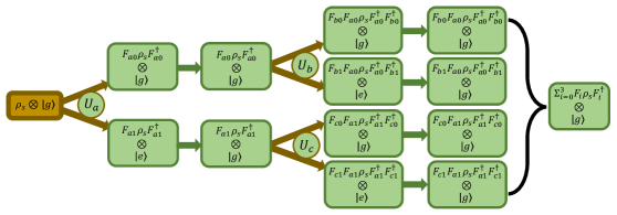
Figure S1: Flowchart illustration of the realization of the strictly incoherent operation (SIO).

III.4 Construction of Two SIOs

The rank-2 strictly incoherent operation (SIO) demonstrated in the main text is given by two Kraus operators

$$E_{0}=\begin{pmatrix}1&0&0&0\\ 0&1&0&0\\ 0&0&0&0\\ 0&0&0&0\end{pmatrix},\quad E_{1}=\begin{pmatrix}0&0&0&0\\ 0&0&0&0\\ 0&0&1&0\\ 0&0&0&1\end{pmatrix}.\quad$$ (S45)

This SIO could be realized directly via a rank-2 AQuO.

The rank-4 SIO is given by four Kraus operators

$$\begin{split}F_{0}=\begin{pmatrix}1&0&0&0\\ 0&0&0&0\\ 0&0&0&0\\ 0&0&0&0\end{pmatrix},\quad F_{1}=\begin{pmatrix}0&0&0&0\\ 0&1&0&0\\ 0&0&0&0\\ 0&0&0&0\end{pmatrix},\quad\\ F_{2}=\begin{pmatrix}0&0&0&0\\ 0&0&0&0\\ 0&0&1&0\\ 0&0&0&0\end{pmatrix},\quad F_{3}=\begin{pmatrix}0&0&0&0\\ 0&0&0&0\\ 0&0&0&0\\ 0&0&0&1\end{pmatrix}.\quad\end{split}$$ (S46)

According to the procedure in the previous section, the rank-4 SIO could be realized adaptively in a two-layer binary-tree construction, as shown by the flowchart in Fig. S1. As an example of the high-rank AQuOs, we provide the details of the operations as follows. For a binary-tree with two layers, there are three unitary gates on the composite system-ancilla:

$$U_{a}=\begin{pmatrix}F_{a0}&*\\ F_{a1}&*\end{pmatrix},\quad$$ (S47)

$$U_{b}=\begin{pmatrix}F_{b0}&*\\ F_{b1}&*\end{pmatrix},\quad$$ (S48)

$$U_{c}=\begin{pmatrix}F_{c0}&*\\ F_{c1}&*\end{pmatrix}.\quad$$ (S49)

Each unitary gate together with a measurement and reset of the ancilla realizes a rank-2 AQuO and the corresponding Kraus operators ({$F_{a0},F_{a1}$}; {$F_{b0},F_{b1}$}; {$F_{c0}$, $F_{c1}$}) in Fig. S1 are given by

$$F_{a0}=\begin{pmatrix}1&0&0&0\\ 0&1&0&0\\ 0&0&0&0\\ 0&0&0&0\end{pmatrix},\quad F_{a1}=\begin{pmatrix}0&0&0&0\\ 0&0&0&0\\ 0&0&1&0\\ 0&0&0&1\end{pmatrix},\quad$$ (S50)

$$F_{b0}=\begin{pmatrix}1&0&0&0\\ 0&0&0&0\\ 0&0&0&0\\ 0&0&0&0\end{pmatrix},\quad F_{b1}=\begin{pmatrix}0&0&0&0\\ 0&1&0&0\\ 0&0&0&0\\ 0&0&0&0\end{pmatrix},\quad$$ (S51)

$$F_{c0}=\begin{pmatrix}0&0&0&0\\ 0&0&0&0\\ 0&0&1&0\\ 0&0&0&0\end{pmatrix},\quad F_{c1}=\begin{pmatrix}0&0&0&0\\ 0&0&0&0\\ 0&0&0&0\\ 0&0&0&1\end{pmatrix}.$$ (S52)

It is easy to verify that $F_{0}=F_{b0}F_{a0}$, $F_{1}=F_{b1}F_{a0}$, $F_{2}=F_{c0}F_{a1}$, $F_{3}=F_{c1}F_{a1}$, and $F_{0},\,F_{1},\,F_{2},\,F_{3}$ are the set of Kraus operators [Eq. (S46)] that represent the target rank-4 SIO [$\varepsilon_{F}(\rho_{s})=\Sigma_{i=0}^{3}F_{i}\rho_{s}F_{i}^{\dagger}$] for the photonic qudit. It is worth noting that the construction of this SIO is equivalent to a projection measurement of the qudit onto the Fock state basis, i.e. the first AQuO implements the measurement to distinguish the subspace $\mathrm{span}\left\{\left|0\right\rangle,\left|1\right\rangle\right\}$ and $\mathrm{span}\left\{\left|2\right\rangle,\left|3\right\rangle\right\}$, while the subsequent AQuOs $\left\{F_{b0},F_{b1}\right\}$ and $\left\{F_{c0},F_{c1}\right\}$ realize the projections on the Fock states.

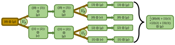
Figure S2: Flowchart illustration of the preparation of the maximally mixed state of the qudit by the AQuO architecture. The composite system-ancilla is initialized to $\left|0\right\rangle\otimes\left|g\right\rangle$.

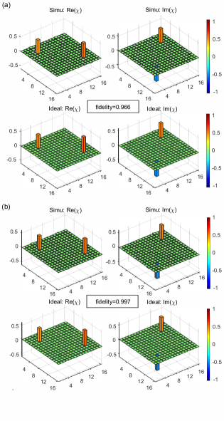
Figure S3: Simulated process fidelity of the odd-parity stabilization operation with (a) and without (b) the ancilla decoherence. Real (left) and imaginary (right) parts of $\chi$ matrix are respectively shown. $\chi_{\mathrm{simu}}$ (top panels) is numerically simulated through QuTip with the experimental pulses and system parameters, while $\chi_{\mathrm{ideal}}$ (bottom panels) is calculated by ideal numerical matrices. The numbers in the $x$ and $y$ axes correspond to the 16 operators which have the same Pauli matrix forms for two qubits but different basis states $\{\left|g\right\rangle\otimes(\left|1\right\rangle,\left|3\right\rangle),\left|e\right\rangle\otimes(\left|1\right\rangle,\left|3\right\rangle)\}$. The color bars represent the value of each matrix element.

III.5 State preparations

In the main text, to show the capability of AQuOs in arbitrary quantum state preparation, we have prepared two typical states, i.e. the maximum coherent state (MCS, $\left|\Psi\right\rangle=\frac{1}{\sqrt{d}}\sum\left|d\right\rangle$) and the maximally mixed state (MMS, $\rho_{s}=\frac{1}{d}\sum_{j=0}^{d}\left|d\right\rangle\left\langle d\right|\equiv\frac{1}{d}\mathbf{I}_{d\times d}$). For the pure state preparation, it could be realized by the previously demonstrated arbitrary unitary gate, by either GRAPE or SNAP Krastanov et al. (2015) approach, that transforms the initially pure state Fock $\left|0\right\rangle$ of the photonic qudit to an MCS $\left|\Psi\right\rangle=\frac{1}{2}(\left|0\right\rangle+\left|1\right\rangle+\left|2\right\rangle+\left|3\right\rangle)$. However, the MMS could not be prepared via unitary gates.

Figure S2 shows a flowchart of the scheme for preparing the MMS. The system is firstly initialized to a pure state of $\left|0\right\rangle\otimes\left|g\right\rangle$ (brown box). Circles represent unitary gates for the rank-2 AQuOs. At the first layer, $U_{A}$ maps the initial state to a pure state $\frac{1}{2}(\left|0\right\rangle+\left|3\right\rangle)\otimes\left|g\right\rangle+\frac{1}{2}(\left|1\right\rangle+\left|2\right\rangle)\otimes\left|e\right\rangle$. Then, the entanglement between the ancilla and the qudit is erased by flipping the ancilla state $\left|e\right\rangle$ to $\left|g\right\rangle$ while keeping $\left|g\right\rangle$ unchanged. After this step, the system is prepared in a mixed state. Then, in the second layer $U_{B}$ or $U_{C}$ is applied adaptively according to the measurement output of the ancilla in the first layer. Here, $U_{B}$ maps state $\frac{1}{\sqrt{2}}(\left|0\right\rangle+\left|3\right\rangle)\otimes\left|g\right\rangle$ to state $\frac{1}{\sqrt{2}}\left|3\right\rangle\otimes\left|g\right\rangle+\frac{1}{\sqrt{2}}\left|0\right\rangle\otimes\left|e\right\rangle$ and $U_{C}$ maps state $\frac{1}{\sqrt{2}}(\left|1\right\rangle+\left|2\right\rangle)\otimes\left|g\right\rangle$ to state $\frac{1}{\sqrt{2}}\left|2\right\rangle\otimes\left|g\right\rangle+\frac{1}{\sqrt{2}}\left|1\right\rangle\otimes\left|e\right\rangle$. By resetting the ancilla to $\left|g\right\rangle$, the final state of the composite system becomes $\rho=\frac{1}{4}\mathbf{I}_{4\times 4}\otimes\left|g\right\rangle\left\langle g\right|$.

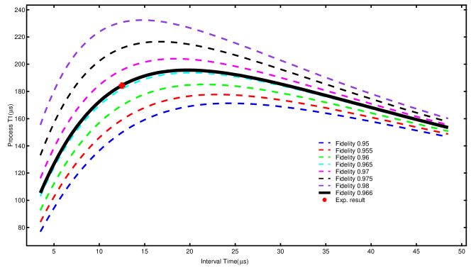
Figure S4: Process fidelity decay time $T_{1}$ of the stabilized odd-parity subspace as a function of the interval time for different gate fidelities.

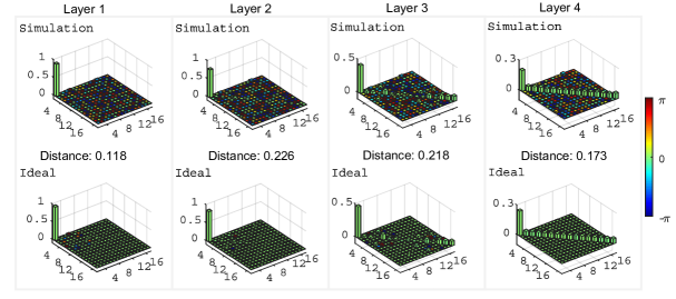
Figure S5: $\chi$ matrix of the 4-level SIC-POVMs at each layer of the binary-tree method. Top panels: $\chi_{\mathrm{simu}}$ is numerically simulated through QuTip with the experimental GRAPE pulses and system parameters including the decoherence. Bottom panels: $\chi_{\mathrm{ideal}}$ is obtained from the numerically simulated ideal AQuO. The height of each matrix bar indicates the absolute value of corresponding element in the $\chi$ matrix, and the color corresponds to the complex angle. Diamond distance between $\chi_{\mathrm{simu}}$ and $\chi_{\mathrm{ideal}}$ at each layer of the binary-tree construction is also shown.

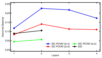
Figure S6: Diamond distance at each layer of the binary-tree construction for different AQuOs.

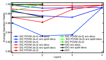
Figure S7: Average operation fidelity at each layer of the binary-tree construction for different AQuOs. Solid dots, hollow dots, and stars respectively correspond to the practical experimental condition including all decoherence and imperfections, the condition excluding the ancilla decoherence, and the condition excluding all decoherence. Different colors represent different AQuOs.

IV Imperfections

IV.1 Optimal interval time for quantum trajectory simulations

In the quantum trajectory simulations, we choose a certain interval and repetitively implement the AQuOs. In principle, the continuous evolution of an open quantum system could be simulated perfectly with ideal unitary operations on the composite system-ancilla with infinitesimal operation time and fast adaptive control. However, in practical experimental system, there is non-negligible decoherence of the ancilla and the photonic qudit. Because of the finite $T_{1}$ and $T_{2}$ of the ancilla, the fidelities of the unitary gates are limited for the GRAPE pulses that are optimized based on an ideal ancilla. Considering the errors of the unitary gates, if we implement AQuOs too frequently with a short interval between sequential AQuOs, significant gate errors would accumulate in the experiments. On the other hand, the qudit would bear more photon loss errors due to energy dissipation if the interval is too long. The trade-off between gate errors and qudit photon loss errors leads to an optimal interval time in the simulation of quantum trajectories. In this section, we systematically investigate the optimal interval via numerical simulations of the experimental procedure including the system decoherence.

Figure S3 shows the simulated fidelities of the unitary gates in the odd-parity stabilization operation with and without the ancilla decoherence in QuTip Johansson et al. (2012, 2013). The process ($\chi$) matrix in Fig. S3 are obtained based on the initial states $\left|g\right\rangle\otimes(\left|0\right\rangle,\left|1\right\rangle,\left|2\right\rangle,\left|3\right\rangle)$ and measured in four bases $\{\left|g\right\rangle\otimes(\left|1\right\rangle,\left|3\right\rangle),\left|e\right\rangle\otimes(\left|1\right\rangle,\left|3\right\rangle)\}$. However, in the presence of decoherence and the imperfection of the GRAPE pulse, the final photonic qudit could have non-negligible leakage to the higher energy levels after the unitary gate, which cannot be detected in the simulation. Therefore, the trace of the obtained output density matrix is smaller than 1. To overcome this problem, we treat the leakage as an appropriate maximally mixed state within the final detection space such that the trace of the output density matrix becomes 1. This treatment of the leakage outside the qudit computational space is valid and similar to the real experiment where the leaked qudit states will be decoded to a mixed state of the ancilla for the final detection. From the numerical results, we conclude that the gate error is mainly attributed to the decoherence of the ancilla qubit, and the resulted gate (process) fidelity is about $96.6\%$.

For the practical implementation of the unitary gates on the composite system-ancilla, a random error occurring during the gate evolution would induce unpredictable and random output due to the complex GRAPE control pulses. Therefore, we could approximate such a decoherence process as a depolarization channel acting on the system with an equal probability for all possible physical errors during the unitary gate. For a $d$-level system, the depolarization channel is given by

$$\mathcal{E}_{\mathrm{dpl}}(\rho) =p\frac{\mathbf{I}_{d\times d}}{d}+\left(1-p\right)\rho,$$ (S53)

where $\mathbf{I}_{d\times d}$ is the $d\times d$ identity matrix and $p$ is the depolarization probability. This indicates that the output is equivalent to replace the quantum state by an MMS with a probability $p$.

Then, the process fidelity of the operation compared with the ideal identity operation is

$$F_{\chi} =\left(1-p\right)\frac{d^{2}-1}{d^{2}}+\frac{1}{d^{2}}$$ (S54)

For our case of $d=4$, the probability of the depolarization channel is given by

$$p =1-(0.966-\frac{1}{16})/\frac{15}{16}=0.036.$$ (S55)

In our experiments, we actually realize an effective operation approximated by $\mathcal{\mathcal{E}_{\mathrm{dpl}}}\circ\mathcal{E}_{\mathrm{Target}}$ when we are targeting to realize an AQuO $\mathcal{E}_{\mathrm{Target}}$. For the quantum trajectory simulations, we repetitively implement the AQuOs with an interval of $t_{\mathrm{int}}$. With $p\ll 1$, the whole dynamics of the system follows the target quantum trajectory evolution, while the system simultaneously couples to a depolarization channel with a rate of $p/t_{\mathrm{int}}$ and a single photon decay channel with a rate of $\kappa_{\mathrm{s}}$, where $\kappa_{\mathrm{s}}$ is the intrinsic decay rate of the storage cavity. So, for the quantum trajectory simulations, there is an optimal interval time that balances the photon decay rate, the dephasing rate $\propto K\kappa_{s}t_{\mathrm{int}}$ induced by the photon decay error and self-Kerr effect ($K$), and the effective depolarization rate $p/t_{\mathrm{int}}$.

To optimize $t_{\mathrm{int}}$, we numerically simulate the process fidelity decay time $T_{1}$ with the above depolarization approximation. Figure S4 shows the process fidelity decay time $T_{1}$ as a function of $t_{\mathrm{int}}$ for different gate fidelities. The black solid line correspondes to a gate fidelity of $96.6\%$ and the red cross correspondes to the experimental result for $t_{\mathrm{int}}=12.5~{}\mathrm{\mu s}$. The simulation results suggest the process fidelity decay time $T_{1}$ could exceed $180~{}\mathrm{\mu s}$ if the optimal interval time around $15~{}\mathrm{\mu s}$ is chosen and a gate fidelity $\geq 96.6\%$ is achieved. In practice, there is also the Kerr effect that would induce extra phases and should be compensated by carefully designing the GRAPE pulses. Therefore, the GRAPE pulse should be numerically optimized for each given interval time. Considering the finite numerical precision and parameter fluctuations in the numerical optimization, there is a fluctuation of the infidelity varying from case to case. Comparing the numerical estimation and the experimental result, the experimental process fidelity decay time $T_{1}=184.3~{}\mathrm{\mu s}$ agrees well with simulation.

IV.2 Process matrix and diamond distance

To characterize the performance of the AQuOs in practical quantum systems, we compare the practical and the ideal $\chi$ matrices of a rank-16 AQuO for a symmetric informationally complete positive operator-valued measure (SIC-POVM) realized in Fig. 3 in the main text. The $\chi$ matrices are obtained after implementing each layer of the binary tree. $\chi_{\mathrm{simu}}$ is numerically simulated through QuTip with the experimental GRAPE pulses and system parameters including the decoherence, while $\chi_{\mathrm{ideal}}$ is obtained from the numerically simulated ideal AQuO. The results are shown in Fig. S5. It is worth mentioning that after implementing the entire four layers of a SIC-POVM we could reconstruct the input quantum state by recording the probability of measuring each POVM element.

In this section, to characterize the performance of the SIC-POVM we treat it as a quantum operation which could be verified by the $\chi$ matrix. Since there are numerical errors in the ideal $\chi$ matrix due to finite numerical precisions, we set the matrix element’s complex angle to be 0 if the element’s absolute value is smaller than $10^{-6}$ for the clarity of the ideal $\chi$ matrix. Comparing the simulated and the ideal matrices, it can be seen that our experimental system could realize the AQuO with small imperfections at each step of the binary-tree implementation.

To quantify the performance of each quantum operation in practice, we evaluate the diamond distance ($D_{\diamond}$) between the numerically simulated ideal AQuO and the physically realizable one. For simplicity, the physically realizable AQuOs are also numerically simulated with the exact experimental pulses and parameters. Then we have

$$D_{\diamond} =||\chi_{\mathrm{simu}}-\chi_{\mathrm{ideal}}||_{\diamond}$$ (S56)

$$=\mathrm{sup}_{\rho}||(\chi_{\mathrm{simu}}\otimes\mathbf{I})(\rho)-(\chi_{\mathrm{ideal}}\otimes\mathbf{I})(\rho)||_{1},$$ (S57)

where the trace norm is defined as

$$||T||_{1}\equiv\mathrm{Tr}\sqrt{T^{\dagger}T}.$$ (S58)

The $D_{\diamond}$ quantifies the difference between two AQuOs as it is related to the upper bound of the success probability

$$p_{\mathrm{succ}}=\frac{1}{2}+\frac{1}{4}D_{\diamond}$$ (S59)

in the single-shot discrimination of two quantum operations by using an ancilla in the discrimination ($0\leq D_{\diamond}\leq 2$). When $D_{\diamond}=2$, the two operations could be perfectly distinguished.

In Fig. S5, the calculated diamond distance between the practically simulated and ideal $\chi$ matrices are labeled. To further study the contribution of the imperfections when realizing AQuOs, $D_{\diamond}$’s of SIC-POVMs for $d=2$, 3 and 4 are also investigated, and the results are summarized in Fig. S6. From the results, we find $D_{\diamond}$ for most operations increases with the number of layers in the binary-tree construction. There are also some extraordinary results: $D_{\diamond}$’s of SIC-POVMs for $d=4$ (blue points) and $d=3$ (red points) decrease when implementing the entire layers of the binary tree. Although there are coherent errors from the pulse imperfections and numerical calculations, we conjecture that these coherent errors will be reduced by the incoherent operations. Based on the process matrix of implementing the SIC-POVM ($\chi$ matrix of entire layers) in Fig. S5, the process of SIC-POVMs corresponds to a depolarization channel which is an incoherent operation. That is the reason for the diamond distance to decrease when implementing entire layers of the binary tree. In Fig. S6, two SIOs (black points) are presented: the implementation of one layer corresponds to the rank-2 SIO with the Kraus operators in Eq. (S45) and implementation of two layers corresponds to the rank-4 SIO with the Kraus operators in Eq. (S46). For comparison, we also show the average operation fidelities

$$\mathcal{F}(\chi_{\mathrm{ideal}},\chi_{\mathrm{simu}})=\left[\mathrm{Tr}\sqrt{\sqrt{\chi_{\mathrm{ideal}}}\chi_{\mathrm{simu}}\sqrt{\chi_{\mathrm{ideal}}}}\right]^{2}$$ (S60)

of different AQuOs in Fig S7.

V State reconstruction and SIC-POVMs

V.1 Density matrix reconstruction

As shown in the main text and also Sec. II.5, the POVM could be realized by recording the outputs of the ancilla with the AQuO architecture. In contrast to many other experiments of POVM, the probabilities of POVM elements acting on state $\rho_{s}$ could all be measured unconditionally by the AQuO setup. Therefore, it is convenient to reconstruct the density matrix of a quantum system $\rho_{s}$ from measurement results of a SIC-POVM, since $\rho_{s}$ can be easily reconstructed by a linear transformation of the probabilities $p_{k}=\mathrm{Tr}(M_{k}\rho_{s})$ from the SIC-POVM $\left\{M_{k}\right\}$. For the schematic shown in Fig. 3(b) in the main text, the system’s SIC-POVM has 16 elements for a qudit with $d=4$. In the experiment, $p_{k}$ directly equals to $p_{ghij}$, the joint probability of the four measurement outcomes of the ancilla in the binary-tree construction. For example, $k=7$ corresponds to $ghij=0111$.

In experiments, a non-positive semi-definite density matrix might be reconstructed from $\left\{p_{k}\right\}$ by the linear transformation due to physical errors. So, maximum likelihood estimation instead of a linear transformation is used in practice to find a set of probabilities $\left\{p_{k}^{\prime}\right\}$, based on which the reconstructed density matrix is Hermitian and positive semi-definite and has the minimum distance from the one based on $\left\{p_{k}\right\}$.

Subjecting the reconstructed density matrix to Hermitian and semi-definite, we evaluate the quantum state fidelity by

$$\mathcal{F}(\rho_{\mathrm{T}},\rho)=\left[\mathrm{Tr}\sqrt{\sqrt{\rho_{\mathrm{T}}}\rho\sqrt{\rho_{\mathrm{T}}}}\right]^{2}.$$ (S61)

Here, $\rho$ is the density matrix derived in experiment and $\rho_{\mathrm{T}}$ is the ideal target density matrix. The relative entropy of coherence is given by

$$\mathcal{C}(\rho)=S(\rho_{\mathrm{diag}})-S(\rho).$$ (S62)

Here, $S$ is the von Neumann entropy and $\rho_{\mathrm{diag}}$ is the state obtained by removing the off-diagonal elements of $\rho$ in the Fock basis Streltsov et al. (2017).

V.2 Calibration of SIC-POVMs

The elements of a SIC-POVM read

$$M_{k}=\frac{1}{d}\left|\phi_{k}\right\rangle\left\langle\phi_{k}\right|,$$ (S63)

where $k\in\{0,1,...,d^{2}\}$ and the basis state $\left|\phi_{i}\right\rangle$ can be generated by operating $d^{2}$ displacement operators on the fiducial vectors Bent et al. (2015), i.e.

$$\left|\phi_{i}\right\rangle=D_{jk}\left|\phi_{f}\right\rangle,$$ (S64)

where $j,k=\{1,2,...,d\}$, $d$ is dimension of system, $\left|\phi_{f}\right\rangle$ is the fiducial state, and $D_{jk}$ is the displacement operator that is given by Bent et al. (2015); Renes et al. (2004)

$$D_{jk}=\omega_{d}^{jk/2}\Sigma_{m}\omega_{d}^{jm}\left|k\oplus m\right\rangle\left\langle m\right|.$$ (S65)

Here, $\omega_{d}=e^{i\frac{2\pi}{d}}$, $\left|m\right\rangle$ is Fock state, and $\bigoplus$ represents the addition modulo $d$. The fiducial vectors (not unique) in our experiment for dimensions $d=2$, 3, 4 are

$$\left|\phi_{f}\right\rangle_{d=2}=\begin{pmatrix}0.8881+0.0000i\\ 0.3251-0.3250i\end{pmatrix},\quad$$ (S66)

$$\left|\phi_{f}\right\rangle_{d=3}=\begin{pmatrix}0.8124+0.0000i\\ 0.1677+0.2911i\\ 0.2386+0.4125i\end{pmatrix},\quad$$ (S67)

and

$$\left|\phi_{f}\right\rangle_{d=4}=\begin{pmatrix}0.2012+0.0000i\\ -0.3076+0.2570i\\ 0.0000+0.4857i\\ -0.1064+0.7427i\end{pmatrix},\quad$$ (S68)

respectively.

To evaluate the performance of a SIC-POVM, we first prepare all basis states, and then characterize these states via the SIC-POVM. Figure S8 shows the experimental results of the state tomography of all basis states by using the SIC-POVM. The average fidelities for all basis states of the SIC-POVM are $96.80\%$, $89.61\%$, and $83.63\%$ for $d=2$, $3$, and $4$, respectively. We notice that the fidelities of some states are higher than the average fidelity of the basis states, and we suppose it is because the probability of measuring the basis state is mostly distributed along only one SIC-POVM element ($25\%$ for $d=4$) while the general states are not the case. For example, the most probability of the measurement outcomes for the MCS ($d=4$) is evenly distributed along four different SIC-POVM elements, while for the MMS the measurement probability is evenly distributed along all SIC-POVM elements. We suppose that a state with more evenly distributed probability of measuring the SIC-POVM elements will be robust against errors in the state reconstruction and tends to have a higher state fidelity.

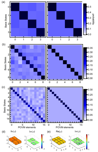
Figure S8: Characterization of SIC-POVMs. (a-c) Characterization of SIC-POVMs for $d=2$, 3, 4: experiment (left) and theory (right). $x$-axis presents different SIC-POVM elements $M_{x}=1/d\left|\phi_{x}\right\rangle\left\langle\phi_{x}\right|$, $y$-axis indicates different prepared basis states $\left|\phi_{y}\right\rangle$, and the color represents the probabilities of prepared states measured along the SIC-POVM elements ($p\left(x,y\right)=\mathrm{Tr}\left[M_{x}\left|\phi_{y}\right\rangle\left\langle\phi_{y}\right|\right]$). (d, e) State tomography of the maximum coherent state for $d=2$ (fidelity is 99.44$\%$) and $d=3$ (fidelity is 95.59$\%$), respectively, by using SIC-POVMs.

V.3 Comparison with Wigner tomography

Conventionally, the states encoded in the storage cavity are characterized by Wigner tomography in the superconducting quantum circuit platform. In this work, we demonstrate the quantum state reconstruction by a SIC-POVM unconditionally, and find that our AQuO approach can greatly save measurement time compared to the conventional approach. Therefore, SIC-POVMs provide an efficient means of quantum state tomography for a quantum system with any finite dimensions Bent et al. (2015); Renes et al. (2004).

Comparing the SIC-POVM and conventional Wigner tomography, the required experimental measurement time of quantum state tomography on a qudit with $d=4$ by a SIC-POVM (about $3$ minutes) is about $200$ times shorter than that by Wigner tomography (about $10$ hours with the same experimental setup). However, the states reconstructed by the SIC-POVM have slightly lower fidelities ($92.52\%$ for the MCS and $98.83\%$ for the MMS) than those by Wigner tomography ($99.57\%$ for the MCS and $99.73\%$ for the MMS). This is because that we use a four-layer binary-tree method to implement the SIC-POVM for the prepared states, and the operation errors accumulate in this process (four steps of rank-2 AQuOs for $d=4$).

References

- Hu et al. (2019) L. Hu, Y. Ma, W. Cai, X. Mu, Y. Xu, W. Wang, Y. Wu, H. Wang, Y. Song, C. Zou, and et al., “Quantum error correction and universal gate set on a binomial bosonic logical qubit,” Nat. Phys. 15, 503 (2019).
- Krastanov et al. (2015) S. Krastanov, V. V. Albert, C. Shen, C.-L. Zou, R. W. Heeres, B. Vlastakis, R. J. Schoelkopf, and L. Jiang, “Universal control of an oscillator with dispersive coupling to a qubit,” Phys. Rev. A 92, 040303 (2015).
- Heeres et al. (2017) R. W. Heeres, P. Reinhold, N. Ofek, L. Frunzio, L. Jiang, M. H. Devoret, and R. J. Schoelkopf, “Implementing a universal gate set on a logical qubit encoded in an oscillator,” Nat. Commun. 8, 94 (2017).
- Khaneja et al. (2005) N. Khaneja, T. Reiss, C. Kehlet, T. Schulte-Herbrüggen, and S. J. Glaser, “Optimal control of coupled spin dynamics: design of nmr pulse sequences by gradient ascent algorithms,” J. Magn. Reson. 172, 296 (2005).
- De Fouquieres et al. (2011) P. De Fouquieres, S. Schirmer, S. Glaser, and I. Kuprov, “Second order gradient ascent pulse engineering,” J. Magn. Reson. 212, 412 (2011).
- Hatridge et al. (2011) M. Hatridge, R. Vijay, D. H. Slichter, J. Clarke, and I. Siddiqi, “Dispersive magnetometry with a quantum limited SQUID parametric amplifier,” Phys. Rev. B 83, 134501 (2011).
- Murch et al. (2013) K. W. Murch, S. J. Weber, C. Macklin, and I. Siddiqi, “Observing single quantum trajectories of a superconducting quantum bit,” Nature 502, 211 (2013).
- Nielsen and Chuang (2000) M. A. Nielsen and I. L. Chuang, Quantum Computation and Quantum Information (Cambridge Univ. Press, 2000).
- Gilchrist et al. (2005) A. Gilchrist, N. K. Langford, and M. A. Nielsen, “Distance measures to compare real and ideal quantum processes,” Phys. Rev. A 71, 062310 (2005).
- (10) The theory of open quantum systems (Oxford University Press on Demand).
- Gardiner and Zoller (2004) C. Gardiner and P. Zoller, Quantum noise: a handbook of Markovian and non-Markovian quantum stochastic methods with applications to quantum optics, Vol. 56 (Springer Science & Business Media, 2004).
- Wiseman and Doherty (2005) H. M. Wiseman and A. C. Doherty, “Optimal unravellings for feedback control in linear quantum systems,” Phys. Rev. Lett. 94, 070405 (2005).
- Andersson and Oi (2008) E. Andersson and D. K. L. Oi, “Binary search trees for generalized measurements,” Phys. Rev. A 77, 052104 (2008).
- Bhandari and Peters (2016) R. Bhandari and N. A. Peters, “On the general constraints in single qubit quantum process tomography,” Sci. Rep. 6, 26004 (2016).
- Touzard et al. (2018) S. Touzard, A. Grimm, Z. Leghtas, S. O. Mundhada, P. Reinhold, C. Axline, M. Reagor, K. Chou, J. Blumoff, and K. M. e. a. Sliwa, “Coherent oscillations inside a quantum manifold stabilized by dissipation,” Phys. Rev. X 8, 021005 (2018).
- Franson et al. (2004) J. D. Franson, B. C. Jacobs, and T. B. Pittman, “Quantum computing using single photons and the zeno effect,” Phys. Rev. A 70, 062302 (2004).
- Shen et al. (2017) C. Shen, K. Noh, V. V. Albert, S. Krastanov, M. H. Devoret, R. J. Schoelkopf, S. M. Girvin, and L. Jiang, “Quantum channel construction with circuit quantum electrodynamics,” Phys. Rev. B 95, 134501 (2017).
- Johansson et al. (2012) J. R. Johansson, P. D. Nation, and F. Nori, “QuTiP: An open-source Python framework for the dynamics of open quantum systems,” Comput. Phys. Commun. 183, 1760 (2012).
- Johansson et al. (2013) J. R. Johansson, P. D. Nation, and F. Nori, “QuTiP 2: A Python framework for the dynamics of open quantum systems,” Comput. Phys. Commun. 184, 1234 (2013).
- Streltsov et al. (2017) A. Streltsov, G. Adesso, and M. B. Plenio, “Colloquium : Quantum coherence as a resource,” Rev. Mod. Phys. 89, 041003 (2017).
- Bent et al. (2015) N. Bent, H. Qassim, A. A. Tahir, D. Sych, G. Leuchs, L. L. Sánchez-Soto, E. Karimi, and R. W. Boyd, “Experimental realization of quantum tomography of photonic qudits via symmetric informationally complete positive operator-valued measures,” Phys. Rev. X 5, 041006 (2015).
- Renes et al. (2004) J. M. Renes, R. Blume-Kohout, A. J. Scott, and C. M. Caves, “Symmetric informationally complete quantum measurements,” J. Math. Phys. 45, 2171 (2004).