Oscillations of 2D ESTER models

Abstract

Context. Recent numerical and theoretical considerations have shown that low-degree acoustic modes in rapidly rotating stars follow an asymptotic formula. In parallel, recent studies have revealed the presence of regular pulsation frequency patterns in rapidly rotating $\delta$ Scuti stars that seem to match theoretical expectations.

Aims. In this context, a key question is whether strong gradients or discontinuities can adversely affect the asymptotic frequency pattern to the point of hindering its identification. Other important questions are how rotational splittings are affected by the 2D rotation profiles expected from baroclinic effects and whether it is possible to probe the rotation profile using these splittings.

Methods. In order to address these questions, we numerically calculate stellar pulsation modes in continuous and discontinuous rapidly rotating models produced by the 2D ESTER (Evolution STEllaire en Rotation) code. This code self-consistently calculates the rotation profile based on baroclinic effects and uses a spectral multi-domain approach, thus making it possible to introduce discontinuities at the domain interfaces without loss of numerical accuracy. The pulsation calculations are carried out using an adiabatic version of the Two-dimensional Oscillation Program (TOP) code. The variational principle is then used to confirm the high numerical accuracy of the pulsation frequencies and to derive an integral formula for the generalised rotational splittings. Acoustic glitch theory, combined with ray dynamics, is applied to the discontinuous models in order to interpret their pulsation spectra.

Results. Our results show that the generalised rotational splittings are very well approximated by the integral formula, except for modes involved in avoided crossings. This potentially allows the application of inverse theory for probing the rotation profile. We also show that glitch theory applied along the island mode orbit can correctly predict the periodicity of the glitch frequency pattern produced by the discontinuity or $\Gamma_{1}$ dip related to the He II ionisation zone in some of the models. Furthermore, the asymptotic frequency pattern remains sufficiently well preserved to potentially allow its detection in observed stars.

1 Introduction

Much effort has gone into producing realistic models of rapidly rotating stars. This includes the pioneering works by Roxburgh et al. (1965), Ostriker & Mark (1968), and Jackson (1970) and continues on in the present with various 1D codes (e.g. Palacios et al. 2003, Eggenberger et al. 2008, Marques et al. 2013) as well as 2D codes such as the one from the Evolution STEllaire en Rotation (ESTER) project (Rieutord & Espinosa Lara 2009, Espinosa Lara & Rieutord 2013, Rieutord et al. 2016). An extensive monograph on the effects of rotation on stellar structure and evolution has also recently been published (Maeder 2009). In parallel, much work has gone into calculating pulsation spectra in such models in order to interpret observations from recent space missions such as CoRoT (Baglin et al. 2009, Auvergne et al. 2009), Kepler (Borucki et al. 2009), and TESS (Ricker et al. 2015). Some of the most recent works include Lovekin & Deupree (2008), Lovekin et al. (2009), Lignières & Georgeot (2008, 2009), Ballot et al. (2010), Reese et al. (2009, 2013), Ouazzani et al. (2015), and Ouazzani et al. (2017). Of these works, only Ouazzani et al. (2015) addresses pulsations in baroclinic stellar models, that is, models in which surfaces of constant pressure, temperature, or density do not coincide. This is a major ingredient of realistic models, as rotating stars are expected to be baroclinic (e.g. Zahn 1992). The work by Ouazzani et al. (2015) used stellar models from Roxburgh (2006) in which the rotation profile is imposed beforehand rather than being calculated in a self-consistent way using energy conservation. In contrast, the ESTER code deduces the rotation profile in a self-consistent way when constructing stellar models. Hence, it is important to study pulsation modes in such models.

One of the first signatures of rotation on stellar pulsations is rotational splittings, the frequency differences between consecutive modes with the same radial order and harmonic degree but different azimuthal orders. At slow rotation rates, rotational splittings can be used to invert 1D or 2D rotation profiles using a first-order perturbative approach (e.g. Deheuvels et al. 2014, Schou et al. 1998, Thompson et al. 2003). At high rotation rates, higher-order effects come into play and must be addressed before meaningful information on the rotation profile can be deduced (e.g. Soufi et al. 1998, Suárez et al. 2009). In this context, a particularly interesting quantity to investigate is the generalised rotational splitting, namely the frequency difference between prograde modes and their retrograde counterparts. In particular, Ouazzani & Goupil (2012) showed that it is possible to distinguish between third-order effects of rotation and latitudinal differential rotation in such splittings. At higher rotation rates, Reese et al. (2009) showed that such splittings are a weighted integral of the rotation profile, provided the degree of differential rotation is not too large. This would potentially provide the basis for carrying out rotation inversions in such stars. This work, however, was restricted to cylindrical rotation profiles and furthermore neglected the influence of the Coriolis force in the integrals. This raises the open questions of whether such weighted integrals can be generalised to general 2D rotation profiles, and if so, how accurate they are.

Another important consideration concerns frequency separations. Indeed, a number of recent studies have shown that the pulsation frequencies of low-degree acoustic modes of rapidly rotating stars follow an asymptotic formula. Such a formula was first explored on an empirical basis (Lignières et al. 2006, Reese et al. 2008, 2009) before being justified using ray dynamics (Lignières & Georgeot 2008, 2009, Pasek et al. 2011, 2012). Reese et al. (2017) studied theoretical pulsation spectra with realistic mode visibilities in rapidly rotating $1.8$ and $2$ M_⊙ stellar models based on the self-consistent field (SCF) method (Jackson et al. 2005, MacGregor et al. 2007). They showed that it may be possible, depending on the configuration, to detect the rotating counterpart to the large frequency separation, or half its value, as well as frequency spacings corresponding to multiples of the rotation rate. More recently, Mirouh et al. (2019) set up a machine learning algorithm to automatically identify to which class a given mode belongs. They went on to characterise the large frequency separation in a large set of models at different rotation rates and with different core compositions (thus mimicking the effects of stellar evolution), and showed a tight scaling relation between it and the stellar mean-density. From an observational point of view, recurrent frequency spacings have been detected in a number of $\delta$ Scuti stars (Mantegazza et al. 2012, Suárez et al. 2014, García Hernández et al. 2009, 2013, Paparó et al. 2016), including a very recent study involving interferometry, spectroscopy, and space photometry (Bouchaud et al. 2020), and interpreted as the large frequency separation or half its value. García Hernández et al. (2015) studied a number of $\delta$ Scuti pulsators in binary systems, for which independent estimates of the mass and radius are available, and have shown that this separation scales with the mean density, as expected based on the calculations in Reese et al. (2008). Ensemble asteroseismology has recently been applied to CoRoT $\delta$ Scuti stars by Michel et al. (2017) who also found regular patterns related to the large separation, although we note that Bowman & Kurtz (2018) applied a similar strategy to Kepler $\delta$ Scuti stars without the same degree of success. Finally, in the very recent work by Bedding et al. (2020), the pulsation spectra of 57 $\delta$ Scuti stars observed by TESS and three by Kepler were matched to axisymmetric $\ell=0$ and $\ell=1$ modes from non-rotating models via echelle diagrams. Such modes were shown to be relatively invariant as a function of rotation rate up to $\sim 0.5\,\Omega_{\mathrm{K}}$ using pulsation calculations in SCF models, apart from a scale factor related to the mean density, thus justifying the use of non-rotating models.

However, it is unclear to what extent the asymptotic formula would hold in the presence of discontinuities within the stellar model. Based on results previously obtained in non-rotating models with sharp gradients (e.g. Monteiro et al. 1994), one can expect the asymptotic formula to still apply albeit with a supplementary oscillatory component. However, it is not clear how strong this component is, how it behaves in the presence of rapid rotation, and whether it can hinder the interpretation of observed oscillation spectra in rapidly rotating stars, as discussed in Breger et al. (2012). The recent works by Bouabid et al. (2013) and Ouazzani et al. (2017) have shown, using the traditional approximation and full 2D pulsation calculations, respectively, how a sharp gradient around the core of rotating $\gamma$ Dor stars affects g-modes. In particular, they show the presence of a periodic component in the period spacings of such modes, analogous to what was found in the non-rotating case (Miglio et al. 2008), in agreement with observations from the Kepler mission (e.g. Van Reeth et al. 2015). Likewise, similar observations in SPB stars have also revealed an oscillatory behaviour in the period spacing of their g-modes (e.g. Pápics et al. 2017). A similar study is needed for acoustic modes in rapidly rotating stars.

In order to address the above questions, we investigate low-degree acoustic modes in rapidly rotating stellar models from the ESTER code. One of the advantages of the ESTER code is its multi-domain spectral approach, ideal for introducing discontinuities while retaining a high numerical accuracy. The pulsation modes are calculated using a multi-domain spectral version of the Two-dimensional Oscillation Program (TOP, Reese et al. 2006, 2009). The article is organised as follows: the following section describes stellar models based on the ESTER code. This is then followed by a description of the pulsation calculations as well as the variational principle, with a particular emphasis on the effects of discontinuities. Section 4 deals with generalised rotational splittings. Section 5 then goes on to describe the effects of discontinuities, both on the pulsation frequencies and on the eigenmodes. This is then followed by the conclusion.

2 Stellar models based on the ESTER code

The aim of the ESTER project is to produce and evolve self-consistent stellar models of rapidly rotating stars. Consequently, a fully 2D approach is used in order to solve the relevant fluid equations while taking into account energy conservation when modelling the stationary structure of the star. This leads to centrifugal deformation of the stellar structure, as well as more subtle effects, namely differential rotation and meridional circulation, resulting from baroclinicity. Consequently, the rotation profile depends on both the radial coordinate and colatitude, and the isobars, isochores, and isotherms are distinct.

In terms of microphysics, it is possible to apply various equations of state (EOS) in ESTER. These include: the ideal gas law with or without radiation pressure, the OPAL EOS (Rogers & Nayfonov 2002), and FreeEOS (Irwin 2012). In what follows, we applied the ideal gas law (without radiation pressure) in the discontinuous models (see below) and one of the continuous models, in order to avoid introducing numerical errors coming from a tabulated EOS, and the OPAL EOS in the other continuous model for the sake of realism. In terms of opacities, there are two options currently implemented: Kramer’s opacities and OPAL opacities (Iglesias & Rogers 1996). We used Kramer’s opacities in conjunction with the ideal gas law to rely entirely on analytical expressions thus reducing numerical errors, and OPAL opacities with the OPAL EOS for the sake of realism and consistency. Models with Kramer’s opacity have significantly larger radii and hence lower mean densities.

Currently, the ESTER code has some limitations. Firstly, it is unable to simulate convective envelopes. Indeed, applying a strong entropy diffusion as is done in the convective core is too approximate for the envelope. Various numerical difficulties have so far prevented the code from converging to a convective solution in such regions. Accordingly, ESTER is currently not suitable for stars with masses below $\sim 1.6$ M_⊙. Secondly, the ESTER code is unable to simulate time evolution using a full chain of nuclear reactions. However, it is possible to alter the core composition in order to mimic the effects of stellar evolution or to include a rudimentary implementation of hydrogen combustion.

From a numerical point of view, the star is divided into multiple domains in the radial direction. There are two main reasons for doing this. First, this allows us to overcome the limitations inherent to using a spectral approach with its imposed collocation grid. In particular, it enables us to have a high resolution near the surface where it is needed. The second reason is that one can place a discontinuity between two domains without losing spectral accuracy. This goes hand in hand with the use of a dedicated coordinate system, $(\zeta,\theta,\phi)$, where $\zeta$ is a surface-fitting radial coordinate that is constant across the stellar surface and across the surfaces which delimit the boundary between consecutive domains (see Rieutord et al. 2016, for more details).

In this study, we use 2 $M_{\odot}$ stellar models at $70\%$ of the Keplerian break-up rotation rate. We note that this value is not too far from the rotation rates of Rasalhague ($\alpha$ Oph) for which $\Omega\sim 0.64\Omega_{\mathrm{K}}$ (see e.g. Deupree 2011, Mirouh et al. 2017, and references therein) and Altair for which $\Omega=0.74\Omega_{\mathrm{K}}$ (Bouchaud et al. 2020), two well-studied $\delta$ Scuti stars with photometric observations from the space missions MOST and WIRE respectively. These models use a spectral approach based on Chebyshev polynomials in the radial direction, and spherical harmonics in the horizontal directions. The radial direction is subdivided into eight domains, the resolution in each domain being 30, 55, 45, 40, 40, 50, 70, and 70, that is, a total of 400 radial points. In the horizontal directions, 22 or 32 points on half of a Gauss-Legendre collocation grid are used depending on the model, thus corresponding to 22 or 32 spherical harmonics with even $\ell$ values. Density discontinuities are achieved by modifying the hydrogen content abruptly. Table 1 gives the characteristics of the five models (Mreal, M, M6, M7, and M7b) involved in this study. In all of the models, $Z=0.02$ everywhere. Figure 1 shows where the discontinuity is located in model M6, and Fig. 2 gives the density and sound velocity profiles in the M, M6, and M7 models.

Table 1: Characteristics of the models used in this study. $X_{\mathrm{int}}$ and $X_{\mathrm{ext}}$ are the hydrogen contents below and above the discontinuity, respectively. $R_{\mathrm{disc}}/R_{\mathrm{eq}}$ gives the equatorial radius at the discontinuity, normalised by the star’s equatorial radius. We note that models Mreal and M are smooth.

Model name	$X_{\mathrm{int}}$	$X_{\mathrm{ext}}$	$R_{\mathrm{disc}}/R_{\mathrm{eq}}$	$\rho_{0}^{+}/\rho_{0}^{-}$	$c_{0}^{+}/c_{0}^{-}$	EOS	Opacities
Mreal	0.70	0.70	n.a.	1	1	OPAL	OPAL
M	0.70	0.70	n.a.	1	1	Ideal gas	Kramer
M6	0.07	0.70	0.857074	0.513889	1.394972	Ideal gas	Kramer
M7	0.07	0.70	0.962678	0.513889	1.394972	Ideal gas	Kramer
M7b	0.70	0.07	0.991861	1.945946	0.716860	Ideal gas	Kramer

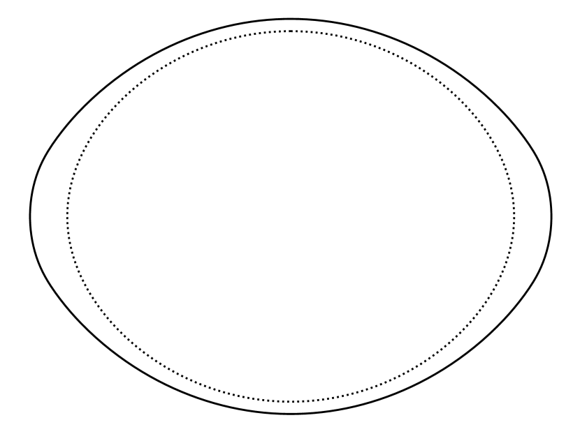
Figure 1: Meridional cross-section of model M6 showing where the discontinuity is located. The other models have a discontinuity closer to the surface.

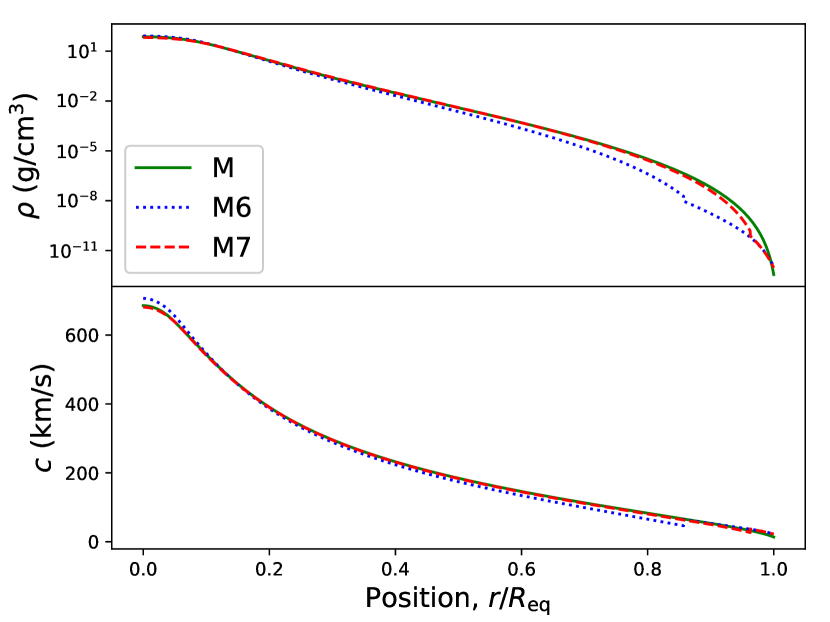
Figure 2: Density (upper panel) and sound velocity (lower panel) profiles along the equator in models M, M6, and M7.

Models Mreal and M are our most realistic models, and serve as a reference, since they do not feature ad hoc discontinuities. Models M6 and M7 include a drop in density near the surface for two different radii, while M7b includes an increase in density near the surface. In realistic models, such as Mreal, such discontinuities are not expected. Instead, more subtle phenomena, such as dips in the $\Gamma_{1}$ profile due to the hydrogen and helium ionisation zones, occur near the stellar surface and can lead to a glitch pattern in the frequencies. However, it is still useful to test models with discontinuities as they exaggerate the phenomena we wish to study, namely acoustic glitches, and should thus make it easier to detect its signature in the pulsation spectrum. Furthermore, one can easily modify the different parameters related to the discontinuity such as depth and intensity in order to study its impact on the frequencies. Finally, the lack of radiation pressure in these models leads to flat $\Gamma_{1}$ profiles meaning that the only glitch signatures expected are those arising from the discontinuities, thus simplifying the subsequent analysis. Nonetheless, the realistic model also allows us to test acoustic glitches related to the $\Gamma_{1}$ profile.

We do note that stars can have a discontinuity around the core due to the depletion of hydrogen by nuclear reactions. However, acoustic modes are sensitive to the near-surface layers of stars and are thus not the most suitable for studying such discontinuities. This is particularly true of island modes as the ray trajectory orbits around which they are concentrated remain far away from the convective core for $\Omega\gtrsim 0.2\,\Omega_{\mathrm{K}}$ (at least for the models in this study). In order to probe such discontinuities, it is more useful to look at gravity-mode glitches (e.g. Miglio et al. 2008, Ouazzani et al. 2017), which is beyond the scope of the present article.

In model M7b, the denser layer is on top. At first sight, this may seem unrealistic, but density inversions can occur in the near-surface layers of stars such as the one shown in Fig. 3 for a $2$ M_⊙ non-rotating main sequence model from grid B of Marques et al. (2008). Such density inversions typically occur as a result of a sharp temperature drop in low density regions of the star (Marques, private communication). Furthermore, including a model with a denser layer on top allows us to test the Snell-Descartes law in different situations.

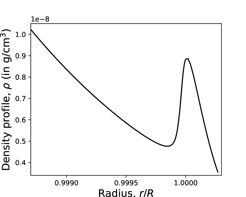
Figure 3: Near-surface density profile in a $2$ M_⊙ non-rotating main sequence model from grid B of Marques et al. (2008).

3 Pulsation calculations

The pulsation modes are calculated using the Two-dimensional Oscillation Program (TOP, Reese et al. 2006, 2009). This program fully takes into account the centrifugal deformation and has been set up to apply a multi-domain spectral approach, in accordance with the models from ESTER. The next subsections describe the set of pulsation equations, the interface conditions that apply between different domains, the boundary conditions, and the numerical approach.

3.1 Pulsation equations

The following set of equations are used to calculate pulsation modes. They are, respectively, the continuity equation, Euler’s equation, the adiabatic relation, and Poisson’s equation:

$$0 = \frac{\delta\rho}{\rho_{0}}+\@vec{\nabla}\cdot\@vec{\xi},$$ (1)

$$0 = \left(\omega+m\Omega\right)^{2}\@vec{\xi}-2i\left(\omega+m\Omega\right)\@vec{\Omega}\times\@vec{\xi}-\@vec{\Omega}\times\left(\@vec{\Omega}\times\@vec{\xi}\right)$$ (2)

$$-\@vec{\xi}\cdot\@vec{\nabla}\left(s\Omega^{2}\@vec{e}_{s}\right)-\frac{P_{0}}{\rho_{0}}\@vec{\nabla}\left(\frac{\delta p}{P_{0}}\right)+\frac{\@vec{\nabla}P_{0}}{\rho_{0}}\left(\frac{\delta\rho}{\rho_{0}}-\frac{\delta p}{P_{0}}\right)-\@vec{\nabla}\Psi$$

$$+\@vec{\nabla}\left(\frac{\@vec{\xi}\cdot\@vec{\nabla}P_{0}}{\rho_{0}}\right)+\left[\frac{\left(\@vec{\xi}\cdot\@vec{\nabla}P_{0}\right)\@vec{\nabla}\rho_{0}-\left(\@vec{\xi}\cdot\@vec{\nabla}\rho_{0}\right)\@vec{\nabla}P_{0}}{\rho_{0}^{2}}\right],$$

$$0 = \frac{\delta p}{P_{0}}-\Gamma_{1}\frac{\delta\rho}{\rho_{0}},$$ (3)

$$0 = \Delta\Psi-\Lambda\left(\rho_{0}\frac{\delta\rho}{\rho_{0}}-\@vec{\xi}\cdot\@vec{\nabla}\rho_{0}\right),$$ (4)

where quantities with the subscript ‘0’ are equilibrium quantities, those with ‘$\delta$’ in front Lagrangian perturbations, $\rho$ the density, $P$ the pressure, $\Psi$ the Eulerian gravitational potential perturbation, $\@vec{\xi}$ the Lagrangian displacement, $\Omega$ the rotation profile (which depends on $\zeta$, the surface-fitting radial coordinate, and $\theta$, the co-latitude), $\Lambda=4\pi G$, $G$ the gravitational constant, $s$ the distance from the rotation axis, and $\@vec{e}_{s}$ the associated unit vector. The term in square brackets (last line of Eq. (2)) does not cancel, since the stellar model is not barotropic. The Lagrangian density perturbation is eliminated in favour of the Lagrangian pressure perturbation using Eq. (3). In the above set of equations, we have neglected the meridional circulation, given that it is expected to have a negligible effect on the pulsation modes.

3.2 Non-dimensionalisation

The following reference length, pressure, and density scales are used:

$$R_{\mathrm{ref}}=R_{\mathrm{eq}},\qquad P_{\mathrm{ref}}=\frac{GM^{2}}{R_{\mathrm{eq}}^{4}},\qquad\rho_{\mathrm{ref}}=\frac{M}{R_{\mathrm{eq}}^{3}},$$ (5)

where $R_{\mathrm{eq}}$ is the equatorial radius and $M$ the mass. As a result of this choice of reference scales, the frequencies are non-dimensionalised by the inverse of the dynamic time scale:

$$\omega_{\mathrm{ref}}=\Omega_{\mathrm{K}}=\sqrt{\frac{GM}{R_{\mathrm{eq}}^{3}}}.$$ (6)

Using this non-dimensionalisation leads to the same set of pulsation equations as previously (Eqs. (1)-(4)) except that $\Lambda$ is now equal to $4\pi$.

3.3 Interface conditions

Given that ESTER models are calculated over multiple domains, interface conditions are needed to describe the relation between various quantities on either side of the different boundaries. Furthermore, care is needed when expressing these conditions given that some of the models contain discontinuities. The first condition is simply that the fluid domain is continuous. In other words, the deformation of the boundary must be the same on either side. This yields the following first order expression:

$$\@vec{\xi}_{-}\cdot\@vec{n}=\@vec{\xi}_{+}\cdot\@vec{n},$$ (7)

where $\@vec{n}$ is the normal to the unperturbed surface, and the subscripts ‘-’ and ‘+’ denote quantities below and above the boundary. This condition does allow the fluid to ‘slip’ along the boundary. A more detailed derivation is given in App. A.1.

A second condition is that the pressure remains continuous across the perturbed boundary. This condition is simply expressed as follows (see App. A.2):

$$\delta p_{-}=\delta p_{+}.$$ (8)

The third condition is the continuity of $\Psi$ and its gradient across the perturbed boundary. This is enforced by the following conditions (see App. A.3):

$$\Psi_{-} = \Psi_{+},$$ (9)

$$\partial_{\zeta}\Psi_{-}+\frac{\Lambda\rho_{-}\zeta^{2}r_{\zeta}}{r^{2}+r_{\theta}^{2}}\xi^{\zeta} = \partial_{\zeta}\Psi_{+}+\frac{\Lambda\rho_{+}\zeta^{2}r_{\zeta}}{r^{2}+r_{\theta}^{2}}\xi^{\zeta}.$$ (10)

3.4 Boundary conditions

As usual, various boundary conditions are needed to complete the system. In the centre, the solutions need to be regular. At the surface, we apply the simple mechanical boundary condition $\delta p=0$. We note that in Reese et al. (2013), a more complex condition was imposed in order to have a non-zero value for $\delta T/T_{0}$ at the surface, useful for mode visibility calculations. However, with such a condition, the pulsation equations do not derive from a variational principle. Here, since we are seeking to obtain accurate frequencies, we prefer the simpler boundary condition ($\delta p=0$), so that we can then apply the variational principle as a supplementary check on the accuracy. Finally, the gravitational potential must match a vacuum potential at infinity. This is achieved by extending the gravitational potential, thanks to Eqs. (9) and (10), into an external domain which encompasses the star and has a spherical outer boundary. The outer boundary condition is then (see Reese et al. 2006):

$$\frac{1}{r_{\zeta}}\frac{\mathrm{d}\Psi_{m}^{\ell}}{\mathrm{d}\zeta}+\frac{\ell+1}{r_{\mathrm{ext}}}\Psi_{m}^{\ell}=0,$$ (11)

where $r_{\zeta}=\partial_{\zeta}r=1-\varepsilon$, $r_{\mathrm{ext}}=2$, and where we have used a harmonic decomposition of $\Psi$, $\ell$ being the spherical harmonic degree.

3.5 Numerical approach

The above system of equations, as well as boundary and interface conditions, are discretised using the spherical harmonic basis for the angular coordinates $(\theta,\phi)$, and using Chebyshev polynomials in the radial direction. This leads to a generalised matrix eigenvalue problem of the form $Ax=\lambda Bx$. This problem is modified using a shift-invert approach to target frequencies around a given shift, $\sigma$, before being solved through the Arnoldi-Chebyshev approach (e.g. Braconnier 1993, Chatelin 2012).

The multi-domain spectral approach used in the radial direction leads to matrices $A$ and $B$ which are block tri-diagonal. The matrix $A-\sigma B$ (which intervenes in the shift-invert approach) can be efficiently factorised using successive factorisations of the diagonal blocks (including a corrective term from the non-diagonal blocks).

3.6 Accuracy of the pulsation calculations

3.6.1 Various numerical resolutions

In order to check the accuracy of the frequencies, it is useful to recalculate the pulsation modes using different radial resolutions or numbers of spherical harmonics. Accordingly, we recalculated $28$ to $30$ axisymmetric ($m=0$) modes in three of the models, using various resolutions. Table 2 gives the maximum relative differences on the pulsation frequencies. The first column corresponds to a $50\,\%$ increase in the number of spherical harmonics in the pulsation calculations, that is, the pulsation modes are calculated with $N_{\theta}=60$ rather $N_{\theta}=40$ spherical harmonics. The second column corresponds to a $\sim 50\,\%$ increase of the radial resolution in the pulsation calculations (after having interpolated the model). Specifically, the resolutions in the eight domains are 45, 85, 70, 60, 60, 75, 105, and 105, that is, a total of $N_{\mathrm{r}}=605$ points. Finally, the third column corresponds to $\sim 50\,\%$ increase of the radial resolution both in the model (that is, the model is calculated with ESTER using an increased radial resolution rather than being interpolated) and pulsation calculations.

Table 2: Maximum relative differences on pulsation frequencies using various resolutions in three of the models.

Model	$1.5\times N_{\theta}$	$1.5\times N_{\mathrm{r}}$	$1.5\times N_{\mathrm{r,\,mod}}$
Mreal	$1.2\times 10^{-5}$	$1.4\times 10^{-8}$	$3.2\times 10^{-5}$
M	$1.2\times 10^{-7}$	$3.4\times 10^{-12}$	$7.6\times 10^{-11}$
M6	$7.9\times 10^{-4}$	$2.8\times 10^{-11}$	–

Two trends can be seen in Table 2. First, modifying the resolution in both the model and the pulsation calculations has a greater impact than only modifying the resolution of the pulsation calculations. This is expected as the higher resolution will be taken into account in the ESTER convergence process when calculating the model in the former case. We note that no value is provided in the last column of Table 2 for model M6 since ESTER was unable to converge in that situation. Secondly, modifying the number of spherical harmonics in the pulsation calculations has a greater impact than modifying the radial resolution. This probably simply illustrates the need for a sufficient harmonic resolution to resolve the intricate island mode geometry, particularly in model M6. Overall, these differences remain small (especially bearing in mind these are the maximal differences), except possibly for the differences related to the harmonic resolution in model M6.

3.6.2 Variational principle

Another way of checking the accuracy of the pulsation calculations consists in comparing the numerical frequencies with those obtained using a variational formula. Such a formula is an integral relation between the frequencies and their associated eigenfunctions. According to the variational principle, the error on the variational frequency scales as the square of the error on the eigenfunctions (e.g. Christensen-Dalsgaard 1982). A general formulation of the variational principle in differentially rotating bodies has previously been obtained by Lynden-Bell & Ostriker (1967). However, the formulation of some of the terms, notably the use of Green’s theorem for the gravitational potential, is not the most suitable for numerical implementation. Previous, numerically-friendly expressions similar to those in Unno et al. (1989), have been obtained in Reese et al. (2006) and Reese et al. (2009), but these expressions were only obtained for uniform or cylindrical rotation profiles, assumed that the star is barotropic, and did not include the effects of discontinuities. In App. B, we give a full derivation for baroclinic models with 2D rotation profiles and discontinuities. The final expression is:

$$0 = \sum_{i}\mathop{{\int}}_{V_{i}}\mathop{{{{{\{}}}}}\left(\omega+m\Omega\right)^{2}\rho_{0}\@vec{\xi}\cdot\@vec{\eta}^{*}-2i\left(\omega+m\Omega\right)\rho_{0}\@vec{\Omega}\cdot\left(\@vec{\xi}\times\@vec{\eta}^{*}\right)$$ (12)

$$-\rho_{0}\left(\@vec{\Omega}\cdot\@vec{\xi}\right)\left(\@vec{\Omega}\cdot\@vec{\eta}^{*}\right)+\rho_{0}\Omega^{2}\@vec{\xi}\cdot\@vec{\eta}^{*}-\@vec{\eta}^{*}\cdot\left[\@vec{\xi}\cdot\@vec{\nabla}\left(\@vec{\nabla}P_{0}\right)\right]$$

$$-\rho_{0}\@vec{\eta}^{*}\cdot\left[\@vec{\xi}\cdot\@vec{\nabla}\left(\@vec{\nabla}\Psi_{0}\right)\right]-\frac{\pi^{*}P}{\Gamma_{1}P_{0}}+\frac{\left(\@vec{\xi}\cdot\@vec{\nabla}P_{0}\right)\left(\@vec{\eta}^{*}\cdot\@vec{\nabla}P_{0}\right)}{\Gamma_{1}P_{0}}\mathop{{{{{\}}}}}}\mathrm{dV}$$

$$+\sum_{i}\int_{S_{i}}\@vec{\xi}\cdot\left(\@vec{\nabla}P_{0}^{-}-\@vec{\nabla}P_{0}^{+}\right)\@vec{\eta}^{*}\cdot\@vec{\mathrm{dS}}+\int_{V_{\infty}}\frac{\@vec{\nabla}\Psi\cdot\@vec{\nabla}\Phi^{*}}{\Lambda}\mathrm{dV},$$

where $\Lambda$ is $4\pi G$ or $4\pi$ in the dimensionless case, $V_{i}$ are the different domains over which the stellar model is continuous, $S_{i}$ are the surfaces of the discontinuities (including the stellar surface), the subscripts ‘$+$’ and ‘$-$’ represent quantities right above and below the discontinuities, respectively ($\@vec{\nabla}P_{0}^{+}=\@vec{0}$ at the stellar surface), and $V_{\infty}$ is infinite space (including the star).

Figure 4 shows the relative differences between the numerical and variational frequencies for our models. In each case a set of 168 modes with quantum numbers $\tilde{n}=19$ to $30$, $\tilde{\ell}=0$ to $1$, $m=-3$ to $3$, was used. We recall that $\tilde{n}$ is the number of nodes along an island mode’s orbit whereas $\tilde{\ell}$ the number of nodes parallel to it. These are related to the usual quantum numbers, $(n,\ell,m)$, of pulsation modes in the non-rotating case via the relations $\tilde{n}=2n+\varepsilon$ and $\tilde{\ell}=\frac{\ell-|m|-\varepsilon}{2}$, where $\varepsilon\equiv\ell+m\,\mathrm{mod}\,2\equiv\tilde{n}\,\mathrm{mod}\,2$ corresponds to the mode’s parity, that is, symmetry with respect to the equatorial plane (Reese 2008). As can be seen in the figure, relative differences range from $10^{-11}$ to $10^{-4}$, apart from an outlier in model M6. This compares quite favourably with the typical accuracy obtained with space missions. For instance, Kepler observations spanned up to four years during the main mission thus leading to a Rayleigh resolution of $0.008\,\mu$Hz. The frequency at maximum amplitude of $\delta$ Scutis can reach approximately $700\,\mu$Hz (e.g. Bowman & Kurtz 2018) thus leading to a relative precision as low as $10^{-5}$ in the best cases. This is higher than the errors on most of the variational frequencies, except for model M6.

The very high accuracy which is reached in a number of cases is due to the use of spectral methods. Such an accuracy was not reached straight away but rather by repeating the calculation using the numerical frequency as the shift, $\sigma$, in the second calculation and refining the solution through supplementary iterations. Factors that decrease the accuracy (even in the second calculations) are the presence of a discontinuity in the stellar model, especially if it is sharp, and the occurrence of avoided crossings which lead to island modes which are ‘polluted’ by contributions from neighbouring modes.

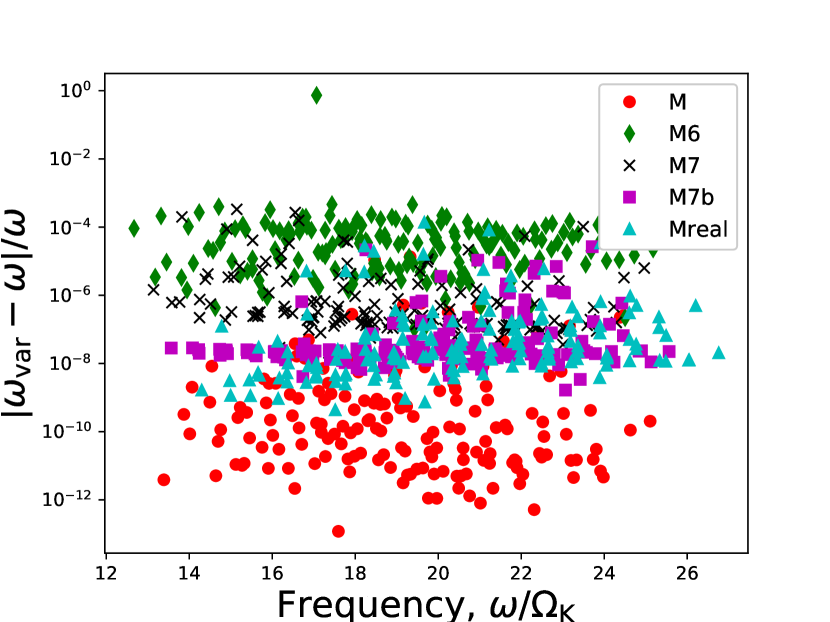
Figure 4: Relative differences between numerical and variational frequencies.

4 Rotation profile

4.1 An approximate rotation kernel

In order to understand the approximate effects of differential rotation on pulsation frequencies, we consider a prograde acoustic mode and its retrograde counterpart. The azimuthal orders of these modes will be denoted $-m$ and $m$, respectively. Furthermore, the subscript ‘+’ will designate the prograde mode and ‘-’ the retrograde mode. The variational principle can be expressed in the following approximate form for these two modes:

$$0\simeq(\omega_{\pm}\mp|m|\Omega_{\pm}^{\mathrm{eff}})^{2}+2(\omega_{\pm}\mp|m|\Omega_{\pm}^{\mathrm{eff}})\mathcal{C}_{\pm}+\mathrm{rest}_{\pm},$$ (13)

where we have used the following definitions/approximations:

$$\Omega_{\pm}^{\mathrm{eff}} = \frac{\int_{V}\Omega\rho_{0}\|\@vec{\xi}_{\pm}\|^{2}dV}{\int_{V}\rho_{0}\|\@vec{\xi}_{\pm}\|^{2}dV},$$ (14)

$$(\Omega_{\pm}^{2})^{\mathrm{eff}} = \frac{\int_{V}\Omega^{2}\rho_{0}\|\@vec{\xi}_{\pm}\|^{2}dV}{\int_{V}\rho_{0}\|\@vec{\xi}_{\pm}\|^{2}dV}\simeq\left(\Omega_{\pm}^{\mathrm{eff}}\right)^{2},$$ (15)

$$\mathcal{C}_{\pm} = \frac{i\int_{V}\rho_{0}\@vec{\Omega}\cdot\left(\@vec{\xi}_{\pm}^{*}\times\@vec{\xi}_{\pm}\right)dV}{\int_{V}\rho_{0}\left\|\@vec{\xi}_{\pm}\right\|^{2}dV},$$ (16)

$$\left(\mathcal{C}_{\pm}\Omega_{\pm}\right)^{\mathrm{eff}} = \frac{i\int_{V}\rho_{0}\Omega\@vec{\Omega}\cdot\left(\@vec{\xi}_{\pm}^{*}\times\@vec{\xi}_{\pm}\right)dV}{\int_{V}\rho_{0}\left\|\@vec{\xi}_{\pm}\right\|^{2}dV}\simeq\mathcal{C}_{\pm}\Omega_{\pm}^{\mathrm{eff}}.$$ (17)

If the two modes are of sufficiently high frequency so that the Coriolis force only has a small impact, and if the rotation profile is not too differential, then the two modes will be close to symmetric. This means that by taking the difference between Eq. 13 applied to the prograde mode, and the same equation applied to the retrograde mode, the terms ‘$\mathrm{rest}_{+}$’ and ‘$\mathrm{rest}_{-}$’ nearly cancel. Neglecting the difference between these two terms leads to the following equation:

$$(\omega_{+}-|m|\Omega_{+}^{\mathrm{eff}})^{2} + 2(\omega_{+}-|m|\Omega_{+}^{\mathrm{eff}})\mathcal{C}_{+}$$ (18)

$$\simeq (\omega_{-}+|m|\Omega_{-}^{\mathrm{eff}})^{2}+2(\omega_{-}+|m|\Omega_{-}^{\mathrm{eff}})\mathcal{C}_{-}.$$

This can be re-expressed as:

$$(\omega_{+}-|m|\Omega_{+}^{\mathrm{eff}})^{2} \left[1+\frac{2\mathcal{C}_{+}}{(\omega_{+}-|m|\Omega_{+}^{\mathrm{eff}})}\right]$$ (19)

$$\simeq (\omega_{-}+|m|\Omega_{-}^{\mathrm{eff}})^{2}\left[1+\frac{2\mathcal{C}_{-}}{(\omega_{-}+|m|\Omega_{-}^{\mathrm{eff}})}\right].$$

Taking the square-root of both sides and assuming $\mathcal{C}_{\pm}\ll(\omega_{\pm}\mp|m|\Omega_{\pm}^{\mathrm{eff}})$ leads to:

$$(\omega_{+}-|m|\Omega_{+}^{\mathrm{eff}}) \left[1+\frac{\mathcal{C}_{+}}{(\omega_{+}-|m|\Omega_{+}^{\mathrm{eff}})}\right]$$ (20)

$$\simeq (\omega_{-}+|m|\Omega_{-}^{\mathrm{eff}})\left[1+\frac{\mathcal{C}_{-}}{(\omega_{-}+|m|\Omega_{-}^{\mathrm{eff}})}\right].$$

This equation can finally be rearranged to yield:

$$\frac{\omega_{+}-\omega_{-}}{2|m|}\simeq\frac{\Omega_{+}^{\mathrm{eff}}+\Omega_{-}^{\mathrm{eff}}}{2}+\frac{-\mathcal{C}_{+}+\mathcal{C}_{-}}{2|m|}.$$ (21)

This equation is particularly interesting because it provides a linear relation between the generalised rotational splitting, which only depends on the frequency of the modes, and the rotation profile. The weighting function that intervenes in the integral is known as the rotation kernel and only depends on the eigenfunctions. If the Coriolis force is neglected, this equation reduces to the linearised version of Eq. (32) from Reese et al. (2009).

Figure 5 shows what a typical rotation kernel will look like for an island mode. As can be seen, the rotation kernel closely follows the geometry of the island mode much like in Reese et al. (2009). Accordingly, these modes are especially sensitive to the rotation rate in this region, in particular near the surface at mid-latitudes.

Figure 5: Rotation kernel for an island mode in model Mreal. The island mode is an $m=1$ mode which is symmetric with respect to the equator and has a frequency of $\nu=760.6\,\mu\mathrm{Hz}$.

In Figs. 6 and 7, we compare the generalised splittings with the right-hand sides of Eq. (21) for models M and Mreal, respectively. The latter is for a much more extensive set of modes. As can be seen, a good agreement is obtained in most cases, but there are some notable exceptions. Such exceptions typically occur for avoided crossings. Indeed, the geometry of the modes changes rapidly as a function of the rotation rate during avoided crossings thereby causing prograde modes and their retrograde counterparts to be at different parts of their avoided crossings and to have different geometric structures. Figure 8 provides an example of such modes. As a result, the terms ‘$\mathrm{rest}_{+}$’ and ‘$\mathrm{rest}_{-}$’ do not cancel each other out. This interpretation is confirmed in Table 3 which provides a detailed comparison between modes in this situation (Solutions 3 and 4) and those which are not undergoing an avoided crossing (Solutions 1 and 2). By including the difference between the terms ‘$\mathrm{rest}_{+}$’ and ‘$\mathrm{rest}_{-}$’ , it is possible to correct Eq. (21) and improve the agreement by a factor of 20 for Solutions 3 and 4. The supplementary rows in this Table also show that the approximations given in Eqs. (15) and (17) are well justified. Hence, apart from the cases involving avoided crossings, the agreement between the generalised splittings and the weighted integrals of the rotation profile (that is, the right-hand side of Eq. (21)) is excellent thus potentially providing the basis for probing the rotation profile via inversions.

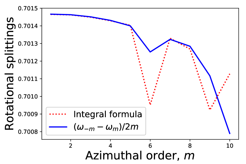
Figure 6: Comparison between generalised rotational splittings and the corresponding weighted integrals of the rotation profile for model M (see Eq. 21).

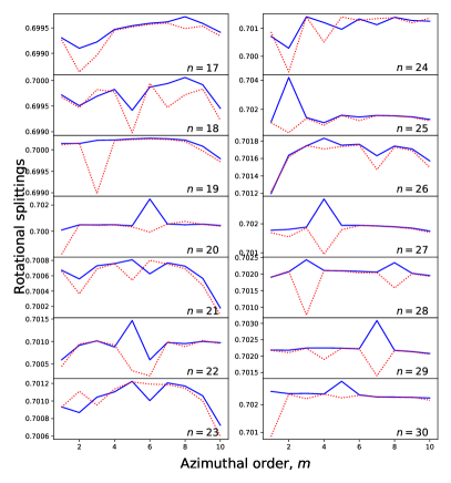
Figure 7: Same as Fig. 6 but for model Mreal and a more extensive set of modes.

Prograde	Retrograde

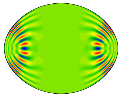
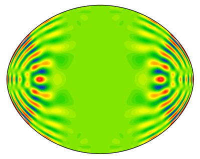
Figure 8: Meridional cross-sections of a prograde mode with $m=-6$ and its retrograde counterpart. The frequencies of these modes are, respectively, $610.2$ and $358.8$ $\mu$Hz. These modes are involved in avoided crossings with other modes (not shown). As a result of being at different stages of the avoided crossing, their geometry is different and applying Eq. (21) yields less accurate results.

Table 3: Generalised splittings versus weighted integrals of the rotation profile, and different terms from Eq. (13) for two pairs of prograde and retrograde modes. $\delta\omega_{\mathrm{var}}/\omega$ corresponds to the relative error on the variational frequency, and $\delta\omega_{\mathrm{var}}^{\mathrm{approx.}}/\omega$ is the same error when $\omega_{\mathrm{var}}$ is calculated using the approximations in Eqs. (15) and (17). The modes from the second pair, Solutions 3 and 4, are undergoing avoided crossings, whereas the other two modes are not.

Quantity	Solution 1	Solution 2	Solution 3	Solution 4
$m$	$-2$	$2$	-6	6
$\omega$	17.50030	14.69444	20.42777	12.01274
$\frac{\omega_{+}-\omega_{-}}{2|m|}$	0.70146		0.70125
$\frac{\Omega_{+}^{\mathrm{eff}}+\Omega_{-}^{\mathrm{eff}}}{2}+\frac{-\mathcal{C}_{+}+\mathcal{C}_{-}}{2|m|}$	0.70146		0.70095
$\delta\omega_{\mathrm{var}}/\omega$	$-8.50\times 10^{-11}$	$-5.18\times 10^{-11}$	$-3.42\times 10^{-10}$	$-1.09\times 10^{-6}$
$\delta\omega_{\mathrm{var}}^{\mathrm{approx.}}/\omega$	$2.01\times 10^{-7}$	$-9.84\times 10^{-8}$	$5.34\times 10^{-7}$	$-4.42\times 10^{-8}$
$\Omega_{\pm}^{\mathrm{eff}}$	0.70463	0.70464	0.70438	0.70436
$\left(\Omega_{\pm}^{2}\right)^{\mathrm{eff}}$	0.49651	0.49652	0.49615	0.49614
$\left(\Omega_{\pm}^{\mathrm{eff}}\right)^{2}$	0.49651	0.49651	0.49615	0.49613
$\mathcal{C}_{\pm}$	-0.04586	-0.05856	-0.03770	-0.07873
$\left(\mathcal{C}_{\pm}\Omega_{\pm}\right)^{\mathrm{eff}}$	-0.03234	-0.04128	-0.02657	-0.05544
$\mathcal{C}_{\pm}\Omega_{\pm}^{\mathrm{eff}}$	-0.03232	-0.04126	-0.02656	-0.05545
rest±	-257.94181	-257.94021	-261.76369	-261.64204

5 Acoustic glitches

We now turn our attention to pulsations in the discontinuous models and focus on acoustic glitches. We recall that glitches are regions in the star with a strong gradient or near discontinuity, which can lead to an oscillatory behaviour in the pulsation spectrum (e.g. Monteiro et al. 1994).

5.1 Frequencies

Figure 9 shows the pulsation frequencies obtained for the various models for modes with $\tilde{n}=19$ to $30$, $\tilde{\ell}=0$ to $1$, and $m=-3$ to $3$. As can be seen, these frequencies follow fairly closely the asymptotic formula given in Reese et al. (2009). However, a closer look reveals irregularities in the pulsation spectra of the discontinuous models. This is brought out more clearly with the frequency separations $\Delta_{\tilde{n}}=\omega_{\tilde{n}+1,\,\tilde{\ell},\,m}-\omega_{\tilde{n},\,\tilde{\ell},\,m}$. In Fig. 10, we plot averaged large separations, $\left<\Delta_{\tilde{n}}\right>=\left<\omega_{\tilde{n}+1,\,\tilde{\ell}}\right>-\left<\omega_{\tilde{n},\,\tilde{\ell}}\right>$, where $\left<\omega_{\tilde{n},\,\tilde{\ell}}\right>$ is the pulsation frequency averaged over the azimuthal orders $m=-3$ to $3$. This is done in order to reduce the effects of avoided crossings which tend to be more numerous in the discontinuous models and tend to mask the frequency variations caused by the glitch. Even then, the averaged large separations in the discontinuous models are more irregular than in the continuous model. This raises the question whether these variations can be explained by glitch theory.

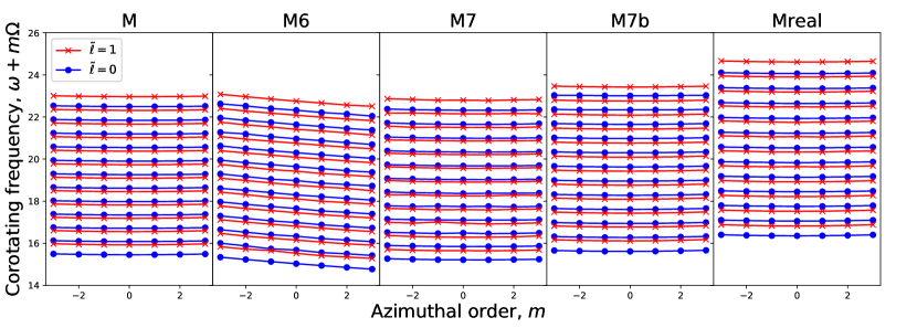
Figure 9: Corotating pulsation frequencies in models M, M6,M7,M7b, and Mreal. These frequencies are fairly well described by the empirical formula from Reese et al. (2009).

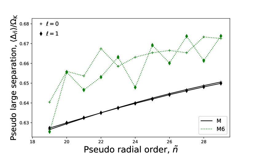
Figure 10: Averaged pseudo large frequency separations, $\left<{\Delta}_{\tilde{n}}\right>$, for the different models.

5.2 Glitch analysis and ray dynamics

In order to investigate the behaviour of the frequencies in a more detailed way, we carried out a simplified ray dynamics analysis. We used the following dispersion relation, valid for axisymmetric modes in the high frequency limit:

$$\omega^{2}=c_{0}^{2}k^{2},$$ (22)

where $k$ is the norm of the wave-vector. A simple reflection was used at the stellar surface, rather than a more realistic but complex approach involving the cut-off frequency (e.g. Lignières & Georgeot 2009). Furthermore, we applied the Snell-Descartes refraction law at the discontinuity:

$$\frac{\sin\vartheta_{+}}{c_{+}}=\frac{\sin\vartheta_{-}}{c_{-}},$$ (23)

where $\vartheta$ is the angle between the surface normal and the wave-vector, $c$ the local sound velocity, and the subscripts ‘$+$’ and ‘$-$’ the upper and lower domains at the discontinuity. We neglect the partial wave reflection at the discontinuity, since we are only searching for the island mode periodic orbit. A more complete description of the ray dynamics is provided in App. C. Figure 11 shows the periodic orbit for island modes superimposed on an island mode in model M6. As can be seen, the orbit reproduces very well the location of the mode.

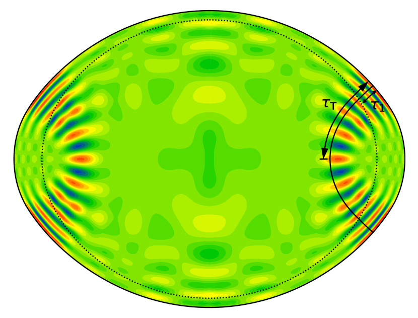
Figure 11: Island mode with periodic orbit superimposed, in model M6. The mode is axisymmetric with a frequency of 309.2 $\mu$Hz. The dotted line shows the location of the discontinuity. The acoustic travel times $\tau_{\mathrm{T}}$ and $\tau_{1}$ along the ray trajectory are illustrated.

Figure 12 then shows the sound velocity, density, and perturbed pressure ($\delta p/\sqrt{P_{0}}$) profiles calculated along the periodic orbit, both as a function of distance along the profile and acoustic travel time. As expected, a sharp transition in wavelength occurs at the discontinuity. Furthermore, when plotted as a function of acoustic travel time, the wave takes on a nearly sinusoidal behaviour as indicated by the comparison with the simple sine curve, apart from a phase shift at the discontinuity and a variable amplitude.

Figure 12: Sound velocity (first row), density (second row), and perturbed pressure ($\delta p/\sqrt{P_{0}}$, third row) profiles as a function of distance (first and second columns) and acoustic travel time (third column) along island periodic orbit. The second column is a zoom of the first column around the first discontinuity. The vertical light blue solid lines indicate the discontinuity and the vertical light blue dotted lines correspond to the equator. The dotted curve in the lower right panel is a simple sine curve with the same periodicity as the mode.

These observations provide the basis for a simple toy model which is described in App. D. According to this model, the frequencies are given to first order by:

$$\omega=\frac{1}{2\tau_{\mathrm{T}}}\left[n\pi+\epsilon\sin\left(n\pi\frac{\tau_{1}}{\tau_{\mathrm{T}}}\right)\right],$$ (24)

where $\tau_{\mathrm{T}}=\int_{\mathrm{surf.}}^{\mathrm{eq.}}\frac{dr}{c}$ is the acoustic travel time from the surface to the equator along the ray path, and $\tau_{1}=\int_{\mathrm{surf.}}^{\mathrm{disc.}}\frac{dr}{c}$, the acoustic travel time from the surface to the discontinuity, as illustrated in Fig. 11. The quantity $\epsilon$ is given by the relation:

$$\epsilon=\frac{k_{-}}{k_{+}}-1=\frac{c_{+}}{c_{-}}-1$$ (25)

and is treated as a small parameter. As shown in App. D, even for $\epsilon=0.39$ (for model M7), Eq. (24) gives an accurate estimate of the glitch period and a rough idea of its amplitude. However, we do not expect the toy model to give an accurate idea of the phase of the glitch pattern on the oscillation frequencies as it would require fully treating surface effects.

Table 4: Acoustic travel times in various models. The quantities $\tau_{\mathrm{T}}$ and $\tau_{1}$ are illustrated in Fig. 11.

Model name	$\tau_{\mathrm{T}}$ (in s)	$\tau_{1}$ (in s)
M	12240.8	–
M6	18330.7	7003.8
M7	16538.4	2153.3
M7b	12676.9	787.9
Mreal	6612.9	670.4

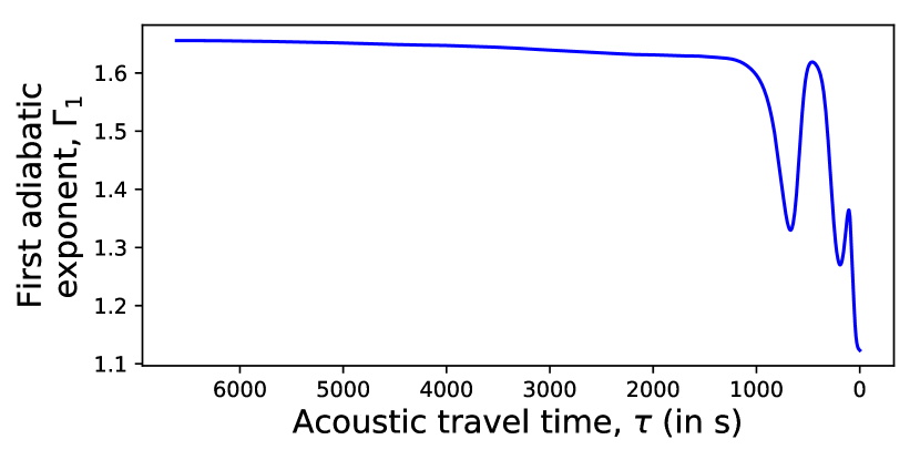
Figure 13: $\Gamma_{1}$ profile in model Mreal along the island mode orbit. The stellar surface corresponds to $\tau=0$ s on the right side, and the intersection of the equatorial plane with the orbit to $\tau=6612.9$ s on the left side.

Table 4 provides the acoustic travel times $\tau_{\mathrm{T}}$ and $\tau_{1}$ for the different models in our study. Although model Mreal is continuous, we included the $\tau_{1}$ value for the He II ionisation zone. Indeed, the $\Gamma_{1}$ profile undergoes a dip in that region, as illustrated in Fig. 13. Based on these values, Fig. 14 compares the predictions from the toy model with the $(\tilde{l},m)=(0,0)$ frequencies minus a second or third-order polynomial fit in order to isolate the glitch pattern. Indeed, using the large separations rather than the frequencies would tend to amplify the impact of avoided crossings thus making it harder to see the glitch pattern. We note that a second rather than third-order polynomial fit was used for model M7b given the relatively long period of the glitch pattern which can be mimicked up to some extent by a third- or higher-order polynomials. An ad hoc phase was added to the glitch pattern from the toy model given that this model is not expected to correctly predict the phase as described above. This allows us to focus on the period and amplitude of the glitch pattern to see how accurate the predictions are.

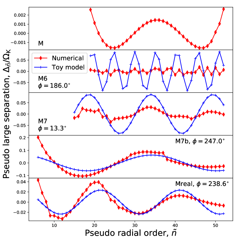
Figure 14: Frequencies of the $(\tilde{\ell},m)=(0,0)$ modes after subtraction of a third-order polynomial fit (or second order polynomial fit in the case M7b) versus the predicted glitch from the toy model. Each panel corresponds to a different model. An ad hoc phase, the value of which is indicated in each panel, has been added to the toy model to improve the agreement.

As can be seen from Fig. 14, a nice agreement is obtained for models M7b, Mreal, and to a lesser extent M7. This confirms that the toy model is able to correctly predict the periodicity of the glitch pattern, at least in some cases. The agreement on the amplitude is satisfactory for M7b but rather poor for M7. For model Mreal, an ad hoc amplitude was used for the predicted glitch pattern. Indeed, the toy model was specifically constructed for discontinuities and is therefore unable to predict the amplitude of the glitch pattern for a smoother transition such as what takes place in an ionisation zone. It is nonetheless interesting to note that the amplitude of this glitch pattern decreases at higher frequencies, as would be expected for such a transition. Model M is not expected to show a glitch pattern since it contains no discontinuities and the $\Gamma_{1}$ profile is very close to $5/3$ throughout the star, as a result of the ideal gas equation of state. The plot shows what is likely to be a fourth order polynomial residual as expected when subtracting a third-order polynomial fit, as confirmed by the much smaller scale of the $y$-axis. In contrast, no agreement is found between the toy model and the glitch pattern for model M6. The reasons for this lack of agreement are not entirely understood, but we do note that most of its island modes are undergoing avoided crossings in contrast to the other models. Avoided crossings typically cause the frequencies to deviate from their asymptotic values and could therefore easily mask a glitch pattern.

5.3 Pulsation mode geometry at the discontinuity

We now investigate in a detailed way the local geometric properties of the islands modes in the region where the periodic orbit intersects the discontinuity. Specifically, we check whether the wave amplitudes match the predictions from a local analysis, and whether the angle between the discontinuity and the orbit matches a numerical estimate based on the island mode.

As recalled in App. E, the pulsation mode including the reflected and refracted waves can locally be approximated as:

$$\left(\frac{\delta p}{P_{0}}\right)^{\pm}=\left[A_{1}^{\pm}\cos(\@vec{k}_{1}^{\pm}\cdot\@vec{x})+A_{2}^{\pm}\cos(\@vec{k}_{2}^{\pm}\cdot\@vec{x})\right]\exp(i\omega t),$$ (26)

where the superscripts ‘$+$’ and ‘$-$’ designate the upper and lower domains, respectively, $\@vec{k}_{1}^{\pm}$ and $\@vec{k}_{2}^{\pm}$ wave vectors, and where the amplitudes, $A_{1}^{\pm}$, $A_{2}^{\pm}$, are related via the relation:

$$\left[\begin{array}[]{c}A_{1}^{+}\\ A_{2}^{+}\end{array}\right]=\frac{1}{2}\left[\begin{array}[]{cc}1+\eta&1-\eta\\ 1-\eta&1+\eta\end{array}\right]\left[\begin{array}[]{c}A_{1}^{-}\\ A_{2}^{-}\end{array}\right],$$ (27)

where

$$\eta=\frac{\rho_{0}^{+}}{\rho_{0}^{-}}\frac{k_{\perp}^{-}}{k_{\perp}^{+}}.$$ (28)

and $k_{\perp}^{\pm}$ is the wave vector component perpendicular to the surface. When $k_{\parallel}\ll k_{\perp}$, the tangential component, the factor $\eta$ reduces to:

$$\eta\simeq\sqrt{\frac{\rho_{0}^{+}}{\rho_{0}^{-}}}=\frac{c_{0}^{-}}{c_{0}^{+}}.$$ (29)

We then investigate several $m=0$ island modes in different models to extract the amplitudes of the refracted and reflected waves and verify the above equations. We start by extracting the $\delta p/P_{0}$ profile as well as its horizontal and vertical gradients, $\@vec{\nabla}_{\parallel}(\delta p/P_{0})$, and $\left(\@vec{\nabla}_{\perp}(\delta p/P_{0})\right)^{\pm}$, just above and below the discontinuity. Since we are focusing on axisymmetric modes, the horizontal gradient is in the meridional plane – there is no component in the $\@vec{e}_{\phi}$ direction. Figure 16 shows a zoom on part of an island mode in model M6 and Fig. 16 shows the extracted profiles. The amplitudes of these profiles are estimated thanks to their maximum absolute values. Given that the $\left(\@vec{\nabla}_{\perp}(\delta p/P_{0})\right)^{\pm}$ profiles have the opposite sign to the $\@vec{\nabla}_{\parallel}(\delta p/P_{0})$ profile, these have negative amplitudes. The tangential wave vector component (which is the same above and below) is estimated by calculating the ratio between the amplitudes of $\@vec{\nabla}_{\parallel}(\delta p/P_{0})$ and $\delta p/P_{0}$. The normal components above and below the discontinuity are obtained via the dispersion relation, thus enforcing Snell-Descartes’ law. The individual wave amplitudes are obtained by calculating appropriate linear combinations of $\left(\@vec{\nabla}_{\perp}(\delta p/P_{0})\right)^{\pm}/k_{\perp}$ and $\left(\@vec{\nabla}_{\parallel}(\delta p/P_{0})\right)/k_{\parallel}$.

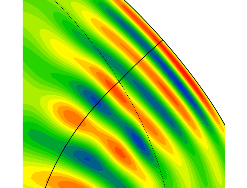
Figure 15: Zoom in on the island mode shown in Fig. 11 (in model M6). The discontinuity is shown using the dotted line, and the solid line corresponds to the island mode orbit. As can be seen, the wavelength decreases just above the discontinuity.

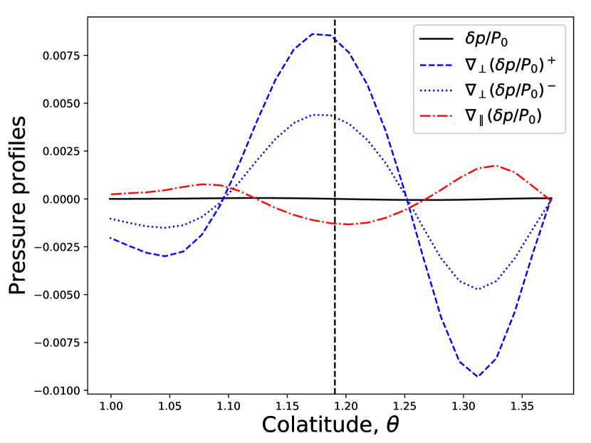
Figure 16: Extracted $\delta p/P_{0}$, $\@vec{\nabla}_{\parallel}(\delta p/P_{0})$, and $\@vec{\nabla}_{\perp}(\delta p/P_{0})^{\pm}$ profiles as a function of $\theta$ along the discontinuity shown in Fig. 16. The vertical dashed line shows colatitude where the island mode periodic orbit crosses the discontinuity.

Table 5 gives the wave vector components and amplitudes for island modes in three of the models. Given that the mode amplitude is arbitrary, we normalised the amplitudes by $A_{2}^{-}$. The quantities ‘$A_{1}^{+}$(theo)’ and ‘$A_{2}^{+}$(theo)’ correspond to the amplitudes deduced from $A_{1}^{-}$ and $A_{2}^{-}$ via Eq. (27). Apart from the $A_{1}^{+}$(theo) for model M6, these values accurately reproduce the numerically obtained amplitudes, $A_{1}^{+}$ and $A_{2}^{+}$, thus showing that the relationship on amplitudes is respected.

Table 5: Wave vector components and amplitudes at the discontinuity for island modes in three of the models.

	M6	M7	M7b
$\omega/\Omega_{\mathrm{K}}$	15.679	15.843	16.276
$c_{+}^{2}$	0.03083	0.01010	0.00201
$c_{-}^{2}$	0.01584	0.00519	0.00391
$k_{\parallel}$	30.480	7.457	5.177
$k_{\perp}^{+}$	83.935	157.434	362.831
$k_{\perp}^{-}$	120.782	219.736	260.074
$k_{\parallel}/k_{\perp}^{+}$	-0.363	-0.0474	-0.0143
$k_{\parallel}/k_{\perp}^{+}$(rays)	-0.260	-0.0369	-0.0078
$k_{\parallel}/k_{\perp}^{-}$	-0.252	-0.0339	-0.0199
$k_{\parallel}/k_{\perp}^{-}$(rays)	-0.184	-0.0264	-0.0109
$A_{1}^{-}$	-0.1475	0.1391	0.4057
$A_{2}^{-}$	1.0000	1.0000	1.0000
$A_{1}^{+}$	0.0061	0.2600	0.2888
$A_{1}^{+}$(theo)	0.0019	0.2608	0.2884
$A_{2}^{+}$	0.8463	0.8791	1.1169
$A_{2}^{+}$(theo)	0.8505	0.8783	1.1173

The quantities $k_{\parallel}$ and $k_{\perp}^{\pm}$ are the horizontal and vertical components of the wave vectors. The quantities $k_{\parallel}/k_{\perp}^{+}$ and $k_{\parallel}/k_{\perp}^{-}$ are given a negative sign since the amplitudes $A_{2}^{\pm}$ (corresponding to the wave vectors $\@vec{k}_{2}^{\pm}=k_{\parallel}\@vec{e}_{\parallel}-k_{\perp}^{\pm}\@vec{e}_{\perp}$) are larger (in absolute value) than the amplitudes $A_{1}^{\pm}$.

Another comparison carried out in Table 5 is between the incidence/departure angles of the wave vectors and the predictions from ray dynamics analysis. The quantities $k_{\parallel}/k_{\perp}^{\pm}$ correspond to the numerically determined values of $\tan\vartheta^{\pm}$ where $\vartheta^{\pm}$ are the angles between the surface normal and the wave vector. The quantities ‘$k_{\parallel}/k_{\perp}^{\pm}$(rays)’ are determined via ray dynamics. A comparison between the two shows some discrepancies but the values remain of the same order. These differences are likely due to the limited accuracy of our approach for extracting the wave vector components, and the fact that the mode behaviour is more complex than what is predicted by ray dynamics.

Finally, as can be seen from the values of $A_{1}^{\pm}$, the amplitudes of the secondary waves, although smaller, is not negligible. Hence, these can be expected to affect the phase shift that occurs at the discontinuity in the primary wave and may possibly lead to increased coupling with other modes due to the modified mode geometry, thereby leading to more avoided crossings.

5.4 Frequency patterns

We now briefly address the question of whether discontinuities can adversely affect frequency patterns to the point of hindering their detection in observed stars. A tool frequently used in solar-like stars is the so-called echelle diagram (e.g. Bedding et al. 2020), in which the frequencies are plotted as a function of the frequencies modulo the large separation. Due to the nearly equidistant frequency patterns in such stars, modes with the same spherical degree line up on vertical ridges in echelle diagrams. In Fig. 17, we produce similar echelle diagrams using the pseudo large separation, $\Delta_{\tilde{n}}$, and only plotting $m=0$ modes for the sake of clarity. Although the discontinuities lead to a more irregular behaviour, clear ridges remain for the different $\tilde{\ell}$ values. Reese et al. (2014) also reached a similar conclusion using histograms of frequency differences for 3 M_⊙ models with discontinuities. Indeed, they found that the pseudo large separation could still be identified in the discontinuous models.

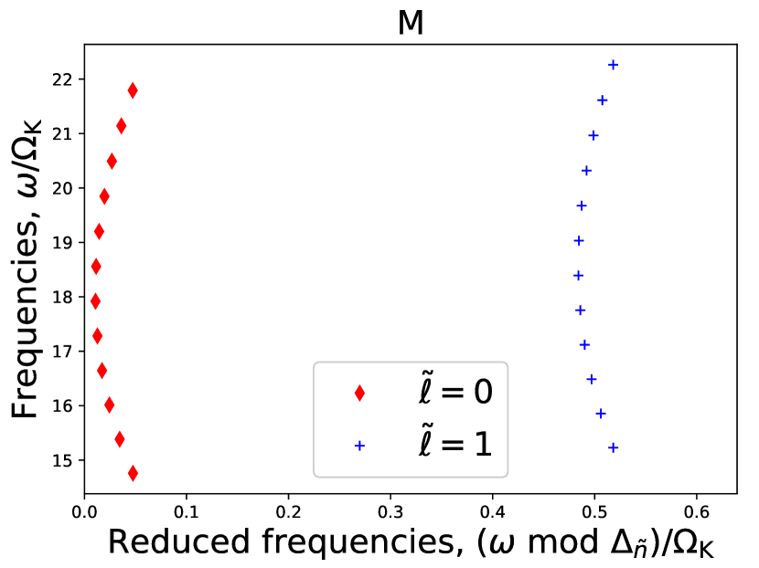
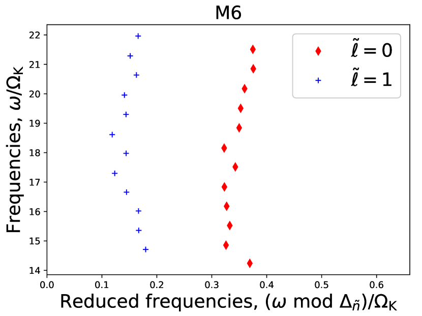
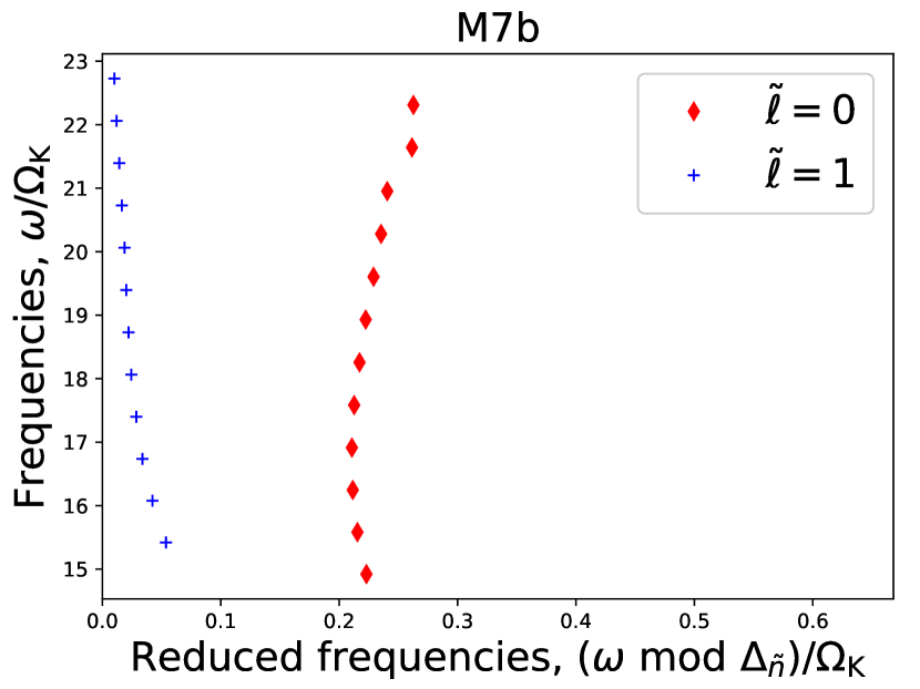
Figure 17: Echelle diagrams for the axisymmetric modes in four of the models.

We also carry out a more quantitative comparison between the pulsation frequencies and a fit based on a simplified version of the asymptotic formula for island mode frequencies (e.g. Reese et al. 2009):

$$\omega=\tilde{n}\Delta_{\tilde{n}}+\tilde{\ell}\Delta_{\tilde{\ell}}+m^{2}\Delta_{\tilde{m}}-m\Omega_{\mathrm{fit}}+\tilde{\alpha},$$ (30)

where $\Delta_{\tilde{n}}$, $\Delta_{\tilde{\ell}}$, $\Delta_{\tilde{m}}$, and $\tilde{\alpha}$ are various parameters related to the stellar structure (Lignières & Georgeot 2009, Pasek et al. 2012), and $\Omega_{\mathrm{fit}}$ an average value of the rotation rate appropriate for the set of modes under consideration. We therefore fit these parameters to reproduce the pulsation spectra of our models for the same set of modes as described in Sect. 3.6.2. Table 6 provides the root mean square differences and maximal differences between the numerical and asymptotic frequencies, normalised by the pseudo large separation, $\Delta_{\tilde{n}}$. As expected, the frequencies of model M are the closest to the asymptotic formula. The mean difference in the realistic model is intermediate between the best and worst model. In terms of maximal differences, model Mreal is among the best whereas model M6 is the worst model, very likely as a result of the increased number of avoided crossings affecting the modes. In all cases, the differences are a few percent of the pseudo large separation (which itself is half the classical large separation), meaning the frequency pattern is still well-preserved and should be possible to identify with a suitable analysis.

Table 6: Root mean square and maximal differences between numerical and asymptotic frequencies for the different models.

Model	$\sqrt{\left<\delta\omega^{2}\right>}/\Delta_{\tilde{n}}$	$\max|\delta\omega|/\Delta_{\tilde{n}}$
M	0.0198	0.0511
M6	0.0282	0.1207
M7	0.0326	0.0855
M7b	0.0224	0.0663
Mreal	0.0273	0.0548

Nonetheless, other factors may hinder finding the above frequency pattern. Indeed, the presence of chaotic modes with their own independent semi-random frequency organisation (Lignières & Georgeot 2009, Evano et al. 2019), or the lack of a clear understanding of the mechanisms responsible for mode selection and pulsation amplitudes both contribute to masking the frequency pattern associated with acoustic island modes.

6 Conclusion

In this work, we calculated, thanks to an adiabatic version of the TOP code, acoustic pulsation modes in rapidly rotating continuous and discontinuous stellar models based on the ESTER code. This allowed us to investigate various topics namely the variational principle for general 2D rotation profiles in discontinuous models, generalised rotational splittings, and acoustic glitches. Some of the important results are:

1. Generalised rotational splittings are well approximated via weighted integrals of the rotation profile using rotation kernels deduced from the variational principle, except for specific cases where avoided crossings lead to discrepancies. This raises the question as to how accurately the rotation profile can be recovered using inverse theory. In a forthcoming article, we plan to investigate this question using a variety of different rotation profiles. In this regard, the automatic mode classification algorithm described in Mirouh et al. (2019) can be used to efficiently identify pairs of prograde-retrograde modes.

2. Discontinuities alter the acoustic frequency patterns, but not to the point of preventing their detection in observed stars (especially taking into account the unrealistic nature of the discontinuities in our models), thus lending credence to recent detections of large frequency separations and ridges in echelle diagrams in $\delta$ Scuti stars (e.g. García Hernández et al. 2015, Bedding et al. 2020). The modifications to the frequency spectrum leads to glitch patterns the periodicity of which can be calculated in a simple way. Nonetheless, the presence of avoided crossings and possibly partial wave reflection at the discontinuity cause deviations from theoretical expectations in some cases. Accordingly, it may be possible to determine acoustic depths of sharp transitions using glitch patterns in observed frequencies.

In a forthcoming work, we plan to investigate acoustic pulsations of ESTER models using a non-adiabatic version of TOP. This will allow us to investigate other topics such as mode excitation and mode behaviour near the stellar surface.

Appendix A Interface conditions

A.1 Domain continuity

In order to ensure that the domain remains continuous, one needs the boundary on either side to be the same. We will now consider a point on the perturbed boundary. This point will be reached by fluid parcels on either side of the boundary. The spatial coordinates of the fluid parcel just below the boundary will be given by the formula:

$$\@vec{r}_{-}+\@vec{\xi}_{-}(\@vec{r}_{-},t).$$ (31)

An analogous formula applies for the spatial coordinates just outside the boundary. This leads to the following matching condition:

$$\@vec{r}_{-}+\@vec{\xi}_{-}(\@vec{r}_{-},t)=\@vec{r}_{+}+\@vec{\xi}_{+}(\@vec{r}_{+},t).$$ (32)

This matching relation is illustrated in Figure 18. It is important to bear in mind that $\@vec{r}_{-}$ is not necessarily equal to $\@vec{r}_{+}$, as illustrated in the figure, since the fluid may slip along either side of the boundary. However, one can rearrange this expression as follows:

$$\@vec{r}_{+}-\@vec{r}_{-}=\@vec{\xi}_{-}(\@vec{r}_{-},t)-\@vec{\xi}_{+}(\@vec{r}_{+},t).$$ (33)

Given that $\@vec{\xi}_{-}$ and $\@vec{\xi}_{+}$ are arbitrarily small, the difference $\@vec{r}_{+}-\@vec{r}_{-}$ is a vector tangent to the surface. Hence, calculating the dot product of the above equation and $\@vec{n}$, the normal to the surface, cancels out the left-hand side and yields:

$$\@vec{\xi}_{-}(\@vec{r}_{-},t)\cdot\@vec{n}=\@vec{\xi}_{+}(\@vec{r}_{+},t)\cdot\@vec{n}.$$ (34)

The difference between $\@vec{\xi}_{+}(\@vec{r}_{+},t)$ and $\@vec{\xi}_{+}(\@vec{r}_{-},t)$ is a second order term. Hence, the above condition reduces to Eq. (7).

Figure 18: Schematic illustration showing the movement of fluid parcels along either side of a boundary that is perturbed by a pulsation mode.

A.2 Condition on the pressure perturbation

The following condition ensures that the pressure remains continuous during the oscillatory movements:

$$P_{\mathrm{Total}}^{-}(\@vec{r}_{-}+\@vec{\xi}_{-},t)=P_{\mathrm{Total}}^{+}(\@vec{r}_{+}+\@vec{\xi}_{+},t),$$ (35)

where we have kept the same notation as above and where $P_{\mathrm{Total}}$ is the total pressure (equilibrium $+$ perturbation). This equation can be developed as follows:

$$P_{0}^{-}(\@vec{r}_{-})+\delta P_{-}(\@vec{r}_{-},t)=P_{0}^{+}(\@vec{r}_{+})+\delta P_{+}(\@vec{r}_{+},t).$$ (36)

We can then use Eq. (32) to develop, say, the right-hand side:

$$P_{0}^{+}(\@vec{r}_{+}) + \delta P_{+}(\@vec{r}_{+},t)$$

$$= P_{0}^{+}(\@vec{r}_{-}+\@vec{\xi}_{-}-\@vec{\xi}_{+})+\delta P_{+}(\@vec{r}_{-}+\@vec{\xi}_{-}-\@vec{\xi}_{+},t)$$

$$\simeq P_{0}^{+}(\@vec{r}_{-})+\left(\@vec{\xi}_{-}-\@vec{\xi}_{+}\right)\cdot\@vec{\nabla}P_{0}^{+}+\delta P_{+}(\@vec{r}_{-},t),$$

where we have neglected second order terms on the third line. Combining this with the previous equation leads to:

$$\delta P_{-}(\@vec{r}_{-},t)-\delta P_{+}(\@vec{r}_{-},t)=\left(\@vec{\xi}_{-}-\@vec{\xi}_{+}\right)\cdot\@vec{\nabla}P_{0}^{+},$$ (37)

where we have used the continuity of the equilibrium pressure. If the boundary coincides with an isobar, the right-hand side of the above equation cancels out because the difference $\@vec{\xi}_{-}-\@vec{\xi}_{+}$ is within the boundary. If the boundary is not an isobar, then in normal circumstances (that is, when the model is continuous), the difference $\@vec{\xi}_{-}-\@vec{\xi}_{+}$ will be $\@vec{0}$. Either way, this leads to the final condition, Eq. (8). There are, however, cases where the right-hand side may not cancel, for instance at the boundary of a convective core with a different chemical composition than the rest of the star. In such a situation, baroclinic flows are set up within the equilibrium model (Espinosa Lara & Rieutord 2013), and probably require setting a specific condition which takes these flows into account. Nonetheless, it is interesting to note that the above condition is in fact symmetric with respect to either side of the boundary. Indeed, the term $\left(\@vec{\xi}_{-}-\@vec{\xi}_{+}\right)\cdot\@vec{\nabla}P_{0}^{+}$ could be replaced by $\left(\@vec{\xi}_{-}-\@vec{\xi}_{+}\right)\cdot\@vec{\nabla}P_{0}^{-}$, since it only involves the gradient of the pressure along the boundary and the pressure is continuous across the boundary.

A.3 Condition on the perturbation to gravitational potential

In much the same way as the pressure, the gravitational potential and its gradient are kept continuous through the following relations:

$$\Psi_{\mathrm{Total}}^{-}(\@vec{r}_{-}+\@vec{\xi}_{-},t) = \Psi_{\mathrm{Total}}^{+}(\@vec{r}_{+}+\@vec{\xi}_{+},t),$$ (38)

$$\@vec{\nabla}\Psi_{\mathrm{Total}}^{-}(\@vec{r}_{-}+\@vec{\xi}_{-},t) = \@vec{\nabla}\Psi_{\mathrm{Total}}^{+}(\@vec{r}_{+}+\@vec{\xi}_{+},t),$$ (39)

where $\Psi_{\mathrm{Total}}$ is the total gravitational potential (equilibrium $+$ perturbation). At this point, however, we will take a different approach than above since we are dealing with the Eulerian rather than Lagrangian perturbation of the gravitational potential. Firstly, the sums $\@vec{r}_{+}+\@vec{\xi}_{+}$ can be replaced by $\@vec{r}_{-}+\@vec{\xi}_{-}$ or vice versa so as to have the same arguments everywhere. Therefore, in what follows we will use the generic notation $\@vec{r}+\@vec{\xi}$ which can be arbitrarily chosen as $\@vec{r}_{-}+\@vec{\xi}_{-}$ or $\@vec{r}_{+}+\@vec{\xi}_{+}$. Developing both sides of both equations, making use of the continuity of the equilibrium gravitational and its gradient to cancel zeroth order terms, and neglecting second order terms lead to the following equations:

$$\Psi_{-}(\@vec{r},t) + \@vec{\xi}(\@vec{r},t)\cdot\@vec{\nabla}\Psi_{0}^{-}(\@vec{r},t)$$ (40)

$$= \Psi_{+}(\@vec{r},t)+\@vec{\xi}(\@vec{r},t)\cdot\@vec{\nabla}\Psi_{0}^{+}(\@vec{r},t),$$

$$\@vec{\nabla}\Psi_{-}(\@vec{r},t) + \@vec{\xi}(\@vec{r},t)\cdot\@vec{\nabla}\left(\@vec{\nabla}\Psi_{0}^{-}(\@vec{r},t)\right)$$ (41)

$$= \@vec{\nabla}\Psi_{+}(\@vec{r},t)+\@vec{\xi}(\@vec{r},t)\cdot\@vec{\nabla}\left(\@vec{\nabla}\Psi_{0}^{+}(\@vec{r},t)\right).$$

Given that $\@vec{\nabla}\Psi_{0}$ is continuous, the first equation reduces to:

$$\Psi_{-}=\Psi_{+}.$$ (42)

In tensorial notation, the left-hand side of the second equation becomes:

$$\partial_{i}\Psi_{-}\@vec{E}^{i}_{-} + \tilde{\xi}^{j}\partial_{j}\left(\@vec{E}^{k}_{-}\partial_{k}\Psi_{0}^{-}\right)$$

$$= \partial_{i}\Psi_{-}\@vec{E}^{i}_{-}+\tilde{\xi}^{j}\left[\partial_{j}\left(\@vec{E}^{k}_{-}\right)\partial_{k}\Psi_{0}^{-}+\@vec{E}^{k}_{-}\partial_{jk}^{2}\Psi_{0}^{-}\right]$$

$$= \partial_{i}\Psi_{-}\@vec{E}^{i}_{-}+\tilde{\xi}^{j}\partial_{j}\left(\@vec{E}^{k}_{-}\right)\partial_{k}\Psi_{0}^{-}+\tilde{\xi}^{j}\partial_{ij}^{2}\Psi_{0}^{-}\@vec{E}^{i}_{-},$$

where $\@vec{E}_{i}$ is the natural basis, $\tilde{\xi}$ the components of $\@vec{\xi}$ over that basis, and $\@vec{E}^{i}$ the dual basis. Calculating the dot product of the above equation with $\@vec{E}_{i}^{-}$ yields:

$$\partial_{i}\Psi_{-}-\tilde{\xi}^{j}{\Gamma\!\!\scriptscriptstyle-}_{ij}^{k}\partial_{k}\Psi_{0}^{-}+\tilde{\xi}^{j}\partial_{ij}^{2}\Psi_{0}^{-},$$ (43)

where $\Gamma_{ij}^{k}=\partial_{i}\left(\@vec{E}_{j}\right)\cdot\@vec{E}^{k}=-\partial_{i}\left(\@vec{E}^{k}\right)\cdot\@vec{E}_{j}$ is the Christoffel symbol of the second kind. With our choice of mapping, only $\Gamma_{\zeta\zeta}^{\zeta}$ is discontinuous across the boundary, hence the notation ${\Gamma\!\!\scriptscriptstyle-}_{\zeta\zeta}^{\zeta}$ and ${\Gamma\!\!\scriptscriptstyle+}_{\zeta\zeta}^{\zeta}$. All of the other geometric quantities ($\@vec{E}_{i}$, $\@vec{E}^{i}$, $\Gamma_{ij}^{k}$ with $(i,j,k)\neq(\zeta,\zeta,\zeta)$) are continuous. Inserting this expression into the left-hand side of Eq. (41) and a similar expression in the right-hand side, and simplifying out continuous terms (geometric, $\Psi_{0}$, and $\@vec{\nabla}\Psi_{0}$) yields the following three relations:

$$\partial_{\zeta}\Psi_{-} + \left(\partial_{\zeta\zeta}^{2}\Psi_{0}^{-}-{\Gamma\!\!\scriptscriptstyle-}_{\zeta\zeta}^{\zeta}\partial_{\zeta}\Psi_{0}\right)\tilde{\xi}^{\zeta}$$ (44)

$$= \partial_{\zeta}\Psi_{+}+\left(\partial_{\zeta\zeta}^{2}\Psi_{0}^{+}-{\Gamma\!\!\scriptscriptstyle+}_{\zeta\zeta}^{\zeta}\partial_{\zeta}\Psi_{0}\right)\tilde{\xi}^{\zeta},$$

$$\partial_{\theta}\Psi_{-} = \partial_{\theta}\Psi_{+},$$ (45)

$$\partial_{\phi}\Psi_{-} = \partial_{\phi}\Psi_{+},$$ (46)

where we have made use of the fact that $\partial_{ij}^{2}\Psi_{0}$ is continuous if $(i,j)\neq(\zeta,\zeta)$. One will in fact notice that the latter two equations are also a direct consequence of Eq. (42).

At this point, it is useful to introduce Poisson’s equation in tensorial notation:

$$\Lambda\rho_{0} = \Delta\Psi_{0}=\@vec{\nabla}\cdot\@vec{\nabla}\Psi_{0}=\partial_{i}\left(\@vec{E}^{j}\partial_{j}\Psi_{0}\right)\cdot\@vec{E}^{i}$$ (47)

$$= g^{ij}\partial_{ij}^{2}\Psi_{0}+\partial_{i}\left(\@vec{E}^{j}\right)\cdot\@vec{E}^{i}\partial_{j}\Psi_{0}$$

$$= g^{ij}\partial_{ij}^{2}\Psi_{0}+\left[\partial_{i}\left(\@vec{E}^{j}\right)\cdot\@vec{E}_{k}\right]\left[\@vec{E}^{i}\cdot\@vec{E}^{k}\right]\partial_{j}\Psi_{0}$$

$$= g^{ij}\partial_{ij}^{2}\Psi_{0}-\Gamma_{ik}^{j}g^{ik}\partial_{j}\Psi_{0}$$

$$= g^{\zeta\zeta}\left(\partial^{2}_{\zeta\zeta}\Psi_{0}-\Gamma_{\zeta\zeta}^{\zeta}\partial_{\zeta}\Psi_{0}\right)+R,$$

where $\Lambda=4\pi G$ or $4\pi$ in the dimensional or dimensionless case, respectively, $g^{ij}=\@vec{E}^{i}\cdot\@vec{E}^{j}$ is the contravariant components of the metric tensor, and $R$ is a sum of terms which are continuous across the boundary. This last expression can then be used to simplify Eq. (44):

$$\partial_{\zeta}\Psi_{-}+\frac{\Lambda\rho_{0}^{-}-R_{-}}{g^{\zeta\zeta}}\tilde{\xi}^{\zeta}=\partial_{\zeta}\Psi_{+}+\frac{\Lambda\rho_{0}^{+}-R_{+}}{g^{\zeta\zeta}}\tilde{\xi}^{\zeta}.$$ (48)

The terms $R_{-}$ and $R_{+}$ cancel out since $R$ is continuous across the boundary. The remaining equation is then

$$\partial_{\zeta}\Psi_{-}+\frac{\Lambda\rho_{0}^{-}\zeta^{2}r_{\zeta}}{r^{2}+r_{\theta}^{2}}\xi^{\zeta}=\partial_{\zeta}\Psi_{+}+\frac{\Lambda\rho_{0}^{+}\zeta^{2}r_{\zeta}}{r^{2}+r_{\theta}^{2}}\xi^{\zeta},$$ (49)

where we have introduced $\xi^{\zeta}$, the $\zeta$ component of $\@vec{\xi}$ on the alternate basis (see, e.g. Eq. 31 of Reese et al. 2006). At this point, it is useful to recall that $\tilde{\xi}^{\zeta}$ and hence $\xi^{\zeta}$ are continuous across the boundary (see Eq. (34)). Hence, using $\@vec{r}_{-}+\@vec{\xi}_{-}$ or $\@vec{r}_{+}+\@vec{\xi}_{+}$ in Eq. (40) leads to the same results.

Appendix B Variational principle

B.1 General formula

In order to derive the variational formula which relates pulsation frequencies and their associated eigenfunctions, we start by calculating the dot product between Euler’s equation (Eq. (2)) and the product of the equilibrium density and the complex conjugate of a second displacement field, $\@vec{\eta}^{*}$, which at this point can be different from $\@vec{\xi}$, and integrate the total over the stellar volume, $V$:

$$0 = \mathop{{\int}}_{V}\mathop{{{\{}}}\left(\omega+m\Omega\right)^{2}\rho_{0}\@vec{\xi}\cdot\@vec{\eta}^{*}\underbrace{-2i\left(\omega+m\Omega\right)\rho_{0}\left(\@vec{\Omega}\times\@vec{\xi}\right)\cdot\@vec{\eta}^{*}}_{I}$$ (50)

$$\underbrace{-\rho_{0}\left[\@vec{\Omega}\times\left(\@vec{\Omega}\times\@vec{\xi}\right)\right]\cdot\@vec{\eta}^{*}}_{II}\underbrace{-\rho_{0}\@vec{\eta}^{*}\cdot\left[\@vec{\xi}\cdot\@vec{\nabla}\left(s\Omega^{2}\@vec{e}_{s}\right)\right]}_{III}$$

$$\underbrace{-P_{0}\@vec{\eta}^{*}\cdot\@vec{\nabla}\left(\frac{\delta p}{P_{0}}\right)}_{IV}\underbrace{+\@vec{\eta}^{*}\cdot\@vec{\nabla}P_{0}\left(\frac{\delta\rho}{\rho_{0}}-\frac{\delta p}{P_{0}}\right)}_{V}$$

$$\underbrace{-\rho_{0}\@vec{\eta}^{*}\cdot\@vec{\nabla}\Psi}_{VI}\underbrace{+\rho_{0}\@vec{\eta}^{*}\cdot\@vec{\nabla}\left(\frac{\@vec{\xi}\cdot\@vec{\nabla}P_{0}}{\rho_{0}}\right)}_{VII}$$

$$\underbrace{+\@vec{\eta}^{*}\cdot\left[\frac{\left(\@vec{\xi}\cdot\@vec{\nabla}P_{0}\right)\@vec{\nabla}\rho_{0}-\left(\@vec{\xi}\cdot\@vec{\nabla}\rho_{0}\right)\@vec{\nabla}P_{0}}{\rho_{0}}\right]}_{VIII}\mathop{{{\}}}}\mathrm{dV}.$$

At this point, the goal is to reformulate the above integral so that it is manifestly symmetric (in a Hermitian sense) with respect to $\@vec{\xi}$ and $\@vec{\eta}$. In what follows, it is very important to bear in mind that $\Omega$ and its associated vector $\@vec{\Omega}=\Omega\@vec{e}_{z}$ depend on $\zeta$ and $\theta$. This is different than the approach taken in Lynden-Bell & Ostriker (1967) where $\Omega$ is constant (differential rotation is, instead, taken into account as a background velocity field, $\@vec{v}_{0}$). Furthermore, given that the equilibrium model may be discontinuous, it will be important, for some of the terms, to decompose the stellar volume into subdomains, $V_{i}$, such that the model is continuous in each subdomain. Obviously, the relation $V=\cup_{i}V_{i}$ holds. Finally, when dealing with the gravitational potential, we will introduce the notation $V_{e}$ to represent an external domain which comprises all of the space outside the star, and $V_{\infty}$ to represent all of space, including the star.

Terms $I$ and $II$ can easily be rearranged into the following symmetric forms:

$$I = \int_{V}-2i\left(\omega+m\Omega\right)\rho_{0}\@vec{\Omega}\cdot\left(\@vec{\xi}\times\@vec{\eta}^{*}\right)\mathrm{dV},$$ (51)

$$II = \int_{V}\left\{-\rho_{0}\left(\@vec{\Omega}\cdot\@vec{\xi}\right)\left(\@vec{\Omega}\cdot\@vec{\eta}^{*}\right)+\rho_{0}\Omega^{2}\@vec{\xi}\cdot\@vec{\eta}^{*}\right\}\mathrm{dV}.$$ (52)

Term $III$ can be rewritten as:

$$III = -\int_{V}\rho_{0}\@vec{\eta}^{*}\cdot\left[\@vec{\xi}\cdot\@vec{\nabla}\left(\frac{\@vec{\nabla}P_{0}}{\rho_{0}}+\@vec{\nabla}\Psi_{0}\right)\right]\mathrm{dV}$$ (53)

$$= \sum_{i}\int_{V_{i}}\left\{\frac{\left(\@vec{\xi}\cdot\@vec{\nabla}\rho_{0}\right)\left(\@vec{\eta}^{*}\cdot\@vec{\nabla}P_{0}\right)}{\rho_{0}}-\@vec{\eta}^{*}\cdot\left[\@vec{\xi}\cdot\@vec{\nabla}\left(\@vec{\nabla}P_{0}\right)\right]\right.$$

$$\left.-\rho_{0}\@vec{\eta}^{*}\cdot\left[\@vec{\xi}\cdot\@vec{\nabla}\left(\@vec{\nabla}\Psi_{0}\right)\right]\right\}\mathrm{dV},$$

where we have made use of the hydrostatic equilibrium equation, in which we have neglected viscosity and meridional circulation. It is important to note that on the second and third line, the integral is carried out over $\sum_{i}V_{i}$. The reason for this is that $\@vec{\nabla}P_{0}$ may be discontinuous, meaning that $\@vec{\nabla}\left(\@vec{\nabla}P_{0}\right)$ has to be calculated over each separate subdomain, $V_{i}$. The last two terms are symmetric. This can be seen, for instance, by expressing them explicitly in terms of their Cartesian coordinates: $\@vec{\eta}^{*}\cdot\left[\@vec{\xi}\cdot\@vec{\nabla}\left(\@vec{\nabla}P_{0}\right)\right]=\left(\eta^{i}\right)^{*}\xi^{j}\partial_{ij}^{2}P_{0}$. The first term cancels out with the last part of term $VIII$.

When developing term $IV$, it is important to treat each domain, $V_{i}$, separately:

$$IV = \sum_{i}\int_{V_{i}}\left\{-\@vec{\nabla}\cdot\left(P_{0}\@vec{\eta}^{*}\frac{\delta p}{P_{0}}\right)+\frac{\delta p}{P_{0}}\@vec{\nabla}\cdot\left(P_{0}\@vec{\eta}^{*}\right)\right\}\mathrm{dV}$$ (54)

$$= -\sum_{i}\int_{B_{i}}\delta P\@vec{\eta}^{*}\cdot\@vec{\mathrm{dS}}+\sum_{i}\int_{V_{i}}\frac{\delta p}{P_{0}}\@vec{\nabla}\cdot\left(P_{0}\@vec{\eta}^{*}\right)\mathrm{dV},$$

where $B_{i}$ denotes the bounds of subdomain $V_{i}$. It turns out that the surface terms cancel out. Indeed, there are two possible cases. In the first case, the surface corresponds to an internal discontinuity. As explained in the previous section, both the normal component of the displacement and the Lagrangian pressure perturbation remain continuous across the discontinuity. Furthermore, there will be two surface terms, one for the domain just below the discontinuity and the other for the domain just above. The vector $\@vec{\mathrm{dS}}$ takes opposite signs in both surface terms since it is directed outwards from the domain. As a result, the two terms cancel. In the second case, the surface term corresponds to the stellar surface. As explained in Sect. 3.4, we impose the simple mechanical boundary condition $\delta p=0$, thereby cancelling this surface term.

Terms $IV$ and $V$ may be combined as follows:

$$IV+V = \sum_{i}\int_{V_{i}}\left[\left(\@vec{\eta}^{*}\cdot\@vec{\nabla}P_{0}\right)\left(\frac{\delta\rho}{\rho_{0}}-\frac{\delta p}{P_{0}}\right)\right.$$ (55)

$$\left.+\left(\@vec{\eta}^{*}\cdot\@vec{\nabla}P_{0}+P_{0}\@vec{\nabla}\cdot\@vec{\eta}^{*}\right)\frac{\delta p}{P_{0}}\right]\mathrm{dV}$$

$$= \sum_{i}\int_{V_{i}}\left[\left(\@vec{\eta}^{*}\cdot\@vec{\nabla}P_{0}\right)\frac{\delta\rho}{\rho_{0}}-\frac{\delta\tilde{\rho}^{*}\delta P}{\rho_{0}}\right]\mathrm{dV},$$

where we have made use of the continuity equation and introduced the Lagrangian density perturbation, $\delta\tilde{\rho}$ associated with $\@vec{\eta}$.

Term $VII$ is treated as follows:

$$VII = \sum_{i}\int_{V_{i}}\left[\@vec{\nabla}\cdot\left(\rho_{0}\@vec{\eta}^{*}\frac{\@vec{\xi}\cdot\@vec{\nabla}P_{0}}{\rho_{0}}\right)-\frac{\@vec{\xi}\cdot\@vec{\nabla}P_{0}}{\rho_{0}}\@vec{\nabla}\cdot\left(\rho_{0}\@vec{\eta}^{*}\right)\right]\mathrm{dV}$$ (56)

$$= \sum_{i}\int_{B_{i}}\left(\@vec{\xi}\cdot\@vec{\nabla}P_{0}\right)\@vec{\eta}^{*}\cdot\@vec{\mathrm{dS}}+\sum_{i}\int_{V_{i}}\left[\left(\@vec{\xi}\cdot\@vec{\nabla}P_{0}\right)\frac{\delta\tilde{\rho}^{*}}{\rho_{0}}\right.$$

$$\left.-\frac{\left(\@vec{\xi}\cdot\@vec{\nabla}P_{0}\right)\left(\@vec{\eta}^{*}\cdot\@vec{\nabla}\rho_{0}\right)}{\rho_{0}}\right]\mathrm{dV},$$

where we have once more made use of the continuity equation. In the above calculations, the surface terms do not cancel, but they are symmetric since both the discontinuities and the stellar surface follow isobars. The term on the last line cancels out with the first part of term $VIII$.

Last but not least, we deal with term $VI$. As has been shown in Unno et al. (1989) and Reese (2006), this term can be rearranged into an integral of the form $\frac{1}{\Lambda}\int_{V_{\infty}}\@vec{\nabla}\Psi\cdot\@vec{\nabla}\Phi^{*}\mathrm{dV}$, where $\Lambda=4\pi G$ or $4\pi$ in the dimensionless case, and $\Phi$ is the gravitational potential associated with the displacement field $\@vec{\eta}$. However, surface terms and terms arising from internal discontinuities were not dealt with in the above works. In what follows, we re-derive this expression, while keeping track of such terms:

$$VI = -\sum_{i}\int_{V_{i}}\@vec{\nabla}\cdot\left(\rho_{0}\@vec{\eta}^{*}\Psi\right)\mathrm{dV}+\sum_{i}\int_{V_{i}}\Psi\@vec{\nabla}\cdot\left(\rho_{0}\@vec{\eta}^{*}\right)\mathrm{dV}$$ (57)

$$= -\sum_{i}\int_{B_{i}}\rho_{0}\Psi\@vec{\eta}^{*}\cdot\@vec{\mathrm{dS}}-\sum_{i}\int_{V_{i}}\Psi\tilde{\rho}^{*}\mathrm{dV}$$

$$= -\sum_{i+e}\int_{B_{i}}\rho_{0}\Psi\@vec{\eta}^{*}\cdot\@vec{\mathrm{dS}}-\frac{1}{\Lambda}\sum_{i+e}\int_{V_{i}}\Psi\Delta\Phi^{*}\mathrm{dV}$$

$$= -\sum_{i+e}\int_{B_{i}}\rho_{0}\Psi\@vec{\eta}^{*}\cdot\@vec{\mathrm{dS}}-\frac{1}{\Lambda}\sum_{i+e}\int_{V_{i}}\@vec{\nabla}\cdot\left(\Psi\@vec{\nabla}\Phi^{*}\right)\mathrm{dV}$$

$$+\frac{1}{\Lambda}\sum_{i+e}\int_{V_{i}}\@vec{\nabla}\Psi\cdot\@vec{\nabla}\Phi^{*}\mathrm{dV}$$

$$= -\sum_{i+e}\int_{B_{i}}\underbrace{\Psi\left(\rho_{0}\@vec{\eta}^{*}+\frac{\@vec{\nabla}\Phi^{*}}{\Lambda}\right)\cdot\@vec{\mathrm{dS}}}_{(a)}+\frac{1}{\Lambda}\sum_{i+e}\int_{V_{i}}\@vec{\nabla}\Psi\cdot\@vec{\nabla}\Phi^{*}\mathrm{dV}$$

$$= \frac{1}{\Lambda}\sum_{i+e}\int_{V_{i}}\@vec{\nabla}\Psi\cdot\@vec{\nabla}\Phi^{*}\mathrm{dV},$$

where $\tilde{\rho}$ is the Eulerian density perturbation associated with $\@vec{\eta}$, the notation ‘$i+e$’ stands for internal domains plus the external domain $V_{e}$. Various steps in the above developments need further explanation. Firstly, on the third line, the external domain was incorporated along with internal domains. This step is justified because the supplementary terms are equal to zero. It must be noted that the surface associated with $V_{e}$, only includes the lower bound, that is, the stellar surface. Secondly, the divergence (or Ostrogradsky’s) theorem was used to transform volume integrals on lines one and four into surface integrals. While straightforward in most cases, it is not as obvious on line four for the external domain $V_{e}$. Indeed, it is not clear if some external boundary at infinity should be included or not. This problem can be dealt with in a rigorous way by considering an external domain, $\tilde{V}_{e}$, which is bounded by a sphere of radius $R_{e}$ and then taking the limit as $R_{e}$ goes to infinity. Such an approach was taken in Reese (2006) who showed that the external surface term goes to zero in such conditions. Finally, it is necessary to show that the surface terms cancel out. We first start by noting that the surface element, $\@vec{\mathrm{dS}}$, is parallel to the vector $\@vec{E}^{\zeta}$, and so may be written as $\tilde{\mathrm{dS}}\@vec{E}^{\zeta}$. Hence, the integrand in the surface terms may be written:

$$(a) = -\Psi\left[\rho_{0}\@vec{\eta}^{*}+\frac{\@vec{\nabla}\Phi^{*}}{\Lambda}\right]\cdot\@vec{E}^{\zeta}\tilde{\mathrm{dS}}$$ (58)

$$= -\Psi\left[\rho_{0}\left(\eta^{\zeta}\right)^{*}+\frac{g^{\zeta j}\partial_{j}\Phi^{*}}{\Lambda}\right]\tilde{\mathrm{dS}}$$

$$= -\Psi\left[\frac{g^{\zeta\zeta}}{\Lambda}\left(\partial_{\zeta}\Phi^{*}+\frac{\Lambda\rho_{0}\left(\eta^{\zeta}\right)^{*}}{g^{\zeta\zeta}}\right)+\frac{g^{\zeta,j\neq\zeta}\partial_{j\neq\zeta}\Phi^{*}}{\Lambda}\right]\tilde{\mathrm{dS}}.$$

Now, we recall that each internal boundary (either from a discontinuity or from the stellar surface) gives rise to two surface terms, one from the domain just below the boundary and the other from the domain just above. As can be seen in the above expression, these two surface terms will cancel out. Indeed, based on the interface conditions (Eqs. (9) and (10)) and the continuity of $g^{ij}$ (for our choice of coordinate system), the first part of the above expression is continuous across the boundary. Only $\tilde{\mathrm{dS}}$ changes signs given that the vector $\@vec{\mathrm{dS}}$ is always directed outwards from the corresponding domain.

We now combine the above formulas to obtain the following expression:

$$0 = \sum_{i}\mathop{{\int}}_{V_{i}}\mathop{{{{{\{}}}}}\left(\omega+m\Omega\right)^{2}\rho_{0}\@vec{\xi}\cdot\@vec{\eta}^{*}-2i\left(\omega+m\Omega\right)\rho_{0}\@vec{\Omega}\cdot\left(\@vec{\xi}\times\@vec{\eta}^{*}\right)$$ (59)

$$-\rho_{0}\left(\@vec{\Omega}\cdot\@vec{\xi}\right)\left(\@vec{\Omega}\cdot\@vec{\eta}^{*}\right)+\rho_{0}\Omega^{2}\@vec{\xi}\cdot\@vec{\eta}^{*}-\@vec{\eta}^{*}\cdot\left[\@vec{\xi}\cdot\@vec{\nabla}\left(\@vec{\nabla}P_{0}\right)\right]$$

$$-\rho_{0}\@vec{\eta}^{*}\cdot\left[\@vec{\xi}\cdot\@vec{\nabla}\left(\@vec{\nabla}\Psi_{0}\right)\right]+\left(\@vec{\eta}^{*}\cdot\@vec{\nabla}P_{0}\right)\frac{\delta\rho}{\rho_{0}}+\left(\@vec{\xi}\cdot\@vec{\nabla}P_{0}\right)\frac{\delta\tilde{\rho}^{*}}{\rho_{0}}$$

$$-\frac{\delta p\delta\tilde{\rho}^{*}}{\rho_{0}}\mathop{{{{{\}}}}}}\mathrm{dV}+\sum_{i}\int_{B_{i}}\left(\@vec{\xi}\cdot\@vec{\nabla}P_{0}\right)\@vec{\eta}^{*}\cdot\@vec{\mathrm{dS}}$$

$$-\int_{S}\delta P\@vec{\eta}^{*}\cdot\@vec{\mathrm{dS}}+\frac{1}{\Lambda}\sum_{i+e}\int_{V_{i}}\@vec{\nabla}\Psi\cdot\@vec{\nabla}\Phi^{*}\mathrm{dV}.$$

We note that at this stage, we have not yet made use of the adiabatic approximation (apart from cancelling out a surface term, thanks to the boundary condition $\delta p=0$, a condition which is usually applied in adiabatic calculations). We now use the adiabatic relation, $\frac{\delta\rho}{\rho_{0}}=\frac{1}{\Gamma_{1}}\frac{\delta p}{P_{0}}$, to replace the Lagrangian density variations by Lagrangian pressure perturbations, and then develop these in terms of Eulerian pressure perturbations and displacement fields. The final result is:

$$0 = \sum_{i}\mathop{{\int}}_{V_{i}}\mathop{{{{{\{}}}}}\left(\omega+m\Omega\right)^{2}\rho_{0}\@vec{\xi}\cdot\@vec{\eta}^{*}-2i\left(\omega+m\Omega\right)\rho_{0}\@vec{\Omega}\cdot\left(\@vec{\xi}\times\@vec{\eta}^{*}\right)$$ (60)

$$-\rho_{0}\left(\@vec{\Omega}\cdot\@vec{\xi}\right)\left(\@vec{\Omega}\cdot\@vec{\eta}^{*}\right)+\rho_{0}\Omega^{2}\@vec{\xi}\cdot\@vec{\eta}^{*}-\@vec{\eta}^{*}\cdot\left[\@vec{\xi}\cdot\@vec{\nabla}\left(\@vec{\nabla}P_{0}\right)\right]$$

$$-\rho_{0}\@vec{\eta}^{*}\cdot\left[\@vec{\xi}\cdot\@vec{\nabla}\left(\@vec{\nabla}\Psi_{0}\right)\right]-\frac{\pi^{*}P}{\Gamma_{1}P_{0}}+\frac{\left(\@vec{\xi}\cdot\@vec{\nabla}P_{0}\right)\left(\@vec{\eta}^{*}\cdot\@vec{\nabla}P_{0}\right)}{\Gamma_{1}P_{0}}\mathop{{{{{\}}}}}}\mathrm{dV}$$

$$+\sum_{i}\int_{B_{i}}\left(\@vec{\xi}\cdot\@vec{\nabla}P_{0}\right)\@vec{\eta}^{*}\cdot\@vec{\mathrm{dS}}+\frac{1}{\Lambda}\sum_{i+e}\int_{V_{i}}\@vec{\nabla}\Psi\cdot\@vec{\nabla}\Phi^{*}\mathrm{dV},$$

where $\pi$ is the Eulerian pressure perturbation associated with the displacement fields $\@vec{\eta}$. This expression is manifestly symmetric in $(\@vec{\xi},P,\Psi)$ and $(\@vec{\eta},\pi,\Phi)$ and consequently leads to the variational principle (Lynden-Bell & Ostriker 1967). A useful consequence of this is the quadratic convergence of the variational frequencies (obtained by assuming that $(\@vec{\xi},P,\Psi)=(\@vec{\eta},\pi,\Phi)$ and solving the above equation for $\omega$) to the true frequency, as a function of the error on the eigenfunctions (e.g. Christensen-Dalsgaard 1982).

B.2 Explicit formulas

In what follows, we provide explicit expressions for the different terms which intervene in Eq. (60), a number of which were already given in Reese et al. (2006). Such expressions are needed when evaluating numerically the variational frequency:

$$\|\@vec{\xi}\|^{2} = |\xi^{\zeta}|^{2}\frac{\zeta^{4}}{r^{4}}+|\xi^{\theta}|^{2}\frac{\zeta^{2}(r^{2}+r_{\theta}^{2})}{r^{4}r_{\zeta}^{2}}+|\xi^{\phi}|^{2}\frac{\zeta^{2}}{r^{2}r_{\zeta}^{2}}$$ (61)

$$+2\Re\left\{\left(\xi^{\zeta}\right)^{*}\xi^{\theta}\right\}\frac{\zeta^{3}r_{\theta}}{r^{4}r_{\zeta}},$$

$$i\@vec{\Omega}\cdot\left(\@vec{\xi}\times\@vec{\xi}^{*}\right) = 2\Omega\left[\left(\frac{\cos\theta}{r_{\zeta}}+\frac{r_{\theta}\sin\theta}{rr_{\zeta}}\right)\frac{\zeta^{2}\left(\xi_{r}^{\theta}\xi_{i}^{\phi}-\xi_{r}^{\phi}\xi_{i}^{\theta}\right)}{r^{2}r_{\zeta}}\right.$$ (62)

$$\left.+\frac{\zeta^{3}\sin\theta\left(\xi_{r}^{\zeta}\xi_{i}^{\phi}-\xi_{r}^{\phi}\xi_{i}^{\zeta}\right)}{r^{3}r_{\zeta}}\right],$$

$$\|\@vec{\nabla}\Psi\|^{2} = \frac{r^{2}+r_{\theta}^{2}}{r^{2}r_{\zeta}^{2}}\left|\partial_{\zeta}\Psi\right|^{2}+\frac{1}{r^{2}}\left|\partial_{\theta}\Psi\right|^{2}+\frac{1}{r^{2}\sin^{2}\theta}\left|\partial_{\phi}\Psi\right|^{2}$$ (63)

$$-\frac{2r_{\theta}}{r^{2}r_{\zeta}}\Re\left(\partial_{\zeta}\Psi^{*}\partial_{\theta}\Psi\right),$$

$$\left|\@vec{\Omega}\cdot\@vec{\xi}\right| = \Omega^{2}\left|\frac{\zeta^{2}r_{\zeta}\cos\theta}{r^{2}r_{\zeta}}\xi^{\zeta}+\frac{\zeta\left(r_{\theta}\cos\theta-r\sin\theta\right)}{r^{2}r_{\zeta}}\xi^{\theta}\right|^{2}.$$ (64)

The term $\@vec{\xi}^{*}\cdot\left[\@vec{\xi}\cdot\@vec{\nabla}\left(\@vec{\nabla}P_{0}\right)\right]$ can be developed through tensor analysis:

$$\@vec{\xi}^{*} \cdot \left[\@vec{\xi}\cdot\@vec{\nabla}\left(\@vec{\nabla}P_{0}\right)\right]$$ (65)

$$= \left(\tilde{\xi}^{j}\right)^{*}\@vec{E}_{j}\cdot\left\{\tilde{\xi}^{i}\partial_{i}\left[\left(\partial_{k}P_{0}\right)\@vec{E}^{k}\right]\right\}$$

$$= \left(\tilde{\xi}^{j}\right)^{*}\@vec{E}_{j}\cdot\left[\tilde{\xi}^{i}\left(\partial_{ik}^{2}P_{0}\right)\@vec{E}^{k}+\tilde{\xi}^{i}\left(\partial_{k}P_{0}\right)\left(\partial_{i}\@vec{E}^{k}\right)\right]$$

$$= \left(\tilde{\xi}^{j}\right)^{*}\tilde{\xi}^{i}\left(\partial_{ij}^{2}P_{0}-\Gamma_{ij}^{k}\partial_{k}P_{0}\right)$$

$$= \frac{\zeta^{4}}{r^{4}r_{\zeta}^{2}}\left(\partial_{\zeta\zeta}^{2}P_{0}-\frac{r_{\zeta\zeta}}{r_{\zeta}}\partial_{\zeta}P_{0}\right)\left|\xi^{\zeta}\right|^{2}$$

$$+\frac{2\zeta^{3}}{r^{4}r_{\zeta}^{2}}\left[\partial_{\zeta\theta}^{2}P_{0}-\left(\frac{r_{\zeta\theta}}{r_{\zeta}}-\frac{r_{\theta}}{r}\right)\partial_{\zeta}P_{0}-\frac{r_{\zeta}}{r}\partial_{\theta}P_{0}\right]\Re\left[\left(\xi^{\zeta}\right)^{*}\xi^{\theta}\right]$$

$$+\frac{\zeta^{2}}{r^{4}r_{\zeta}^{2}}\left(\partial_{\theta\theta}^{2}P_{0}-\frac{rr_{\theta\theta}-2r_{\theta}^{2}-r^{2}}{rr_{\zeta}}\partial_{\zeta}P_{0}-\frac{2r_{\theta}}{r}\partial_{\theta}P_{0}\right)\left|\xi^{\theta}\right|^{2}$$

$$+\frac{\zeta^{2}}{r^{4}r_{\zeta}^{2}}\left(\frac{r-r_{\theta}\cot\theta}{r_{\zeta}}\partial_{\zeta}P_{0}+\cot\theta\partial_{\theta}P_{0}\right)\left|\xi^{\phi}\right|^{2},$$

where we have expressed the displacement using the alternate components on the last line.

Appendix C Ray dynamics

Ray trajectories were calculated in the usual spherical coordinate system $(r,\theta,\phi)$ using the system of equations provided in Prat et al. (2016). We used $H=\omega^{2}=c_{0}^{2}k^{2}$ as the Hamiltonian function. This leads to the following system:

$$\frac{\mathrm{d}r}{\mathrm{d}t} = \frac{\partial H}{\partial k_{r}}=2c_{0}^{2}k_{r},$$ (66)

$$\frac{\mathrm{d}\theta}{\mathrm{d}t} = \frac{1}{r}\frac{\partial H}{\partial k_{\theta}}=\frac{2c_{0}^{2}k_{\theta}}{r},$$ (67)

$$\frac{\mathrm{d}k_{r}}{\mathrm{d}t} = -\frac{\partial H}{\partial r}+\frac{k_{\theta}}{r}\frac{\partial H}{\partial k_{\theta}}=-k^{2}\left(\frac{\partial c_{0}^{2}}{\partial r}\right)_{\theta}+\frac{2c_{0}^{2}k_{\theta}^{2}}{r},$$ (68)

$$\frac{\mathrm{d}k_{\theta}}{\mathrm{d}t} = -\frac{1}{r}\frac{\partial H}{\partial\theta}+\frac{k_{\theta}}{r}\frac{\partial H}{\partial k_{r}}=-\frac{k^{2}}{r}\left(\frac{\partial c_{0}^{2}}{\partial\theta}\right)_{r}+\frac{2c_{0}^{2}k_{r}k_{\theta}}{r}.$$ (69)

Although the ray trajectories are calculated in the spherical coordinate system, the various derivatives of $c_{0}^{2}$ are first calculated in the spheroidal coordinate system before being converted to the spherical system via the following relations:

$$\left(\frac{\partial c_{0}^{2}}{\partial r}\right)_{\theta} = \frac{1}{r_{\zeta}}\left(\frac{\partial c_{0}^{2}}{\partial\zeta}\right)_{\theta},$$ (70)

$$\left(\frac{\partial c_{0}^{2}}{\partial\theta}\right)_{r} = \left(\frac{\partial c_{0}^{2}}{\partial\theta}\right)_{\zeta}-\frac{r_{\theta}}{r_{\zeta}}\left(\frac{\partial c_{0}^{2}}{\partial\zeta}\right)_{\theta}.$$ (71)

The system of equations (66) to (69) is solved numerically for an initial position and wave vector using a fourth order Runge-Kutta method, except near discontinuities and the stellar surface where Heun’s third-order method (also a Runge-Kutta method) is used instead. Indeed at these locations, the step is adjusted so as to fall precisely on the relevant boundary, thus making it easier to apply a wave reflection or Snell-Descartes’ law, and the use of Heun’s method reduces the risk of overstepping this boundary, unlike the fourth order Runge-Kutta method.

Appendix D Toy model for glitches

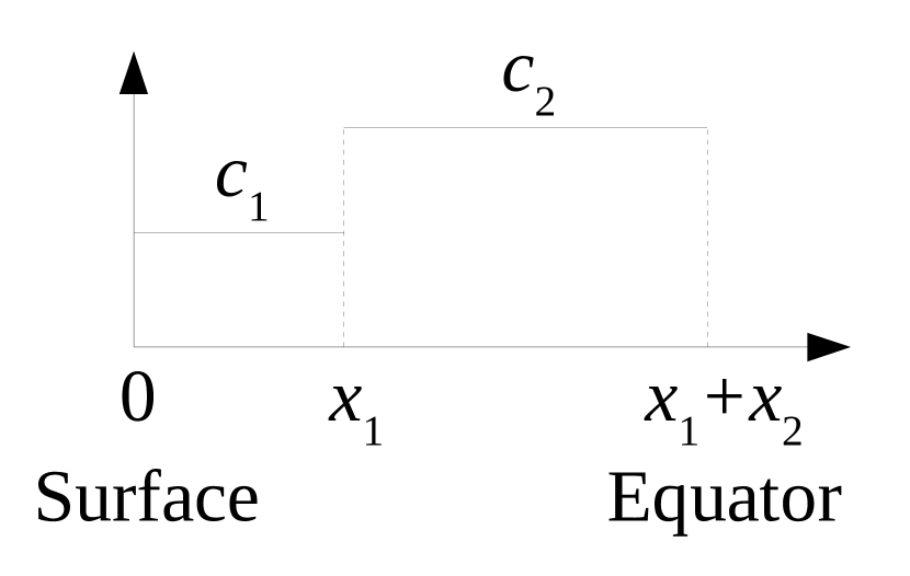
Figure 19: Sound velocity profile in toy model. Only half the model is shown, the other half (beyond the centre, that is, $x_{1}+x_{2}$) being symmetric.

In this section, we consider a 1D toy model representative of a sound wave travelling along an island mode ray path in the presence of a discontinuity. Figure 19 illustrates half of this model, the other half being deduced by symmetry. For the sake of simplicity, constant sound velocities, denoted $c_{1}$ and $c_{2}$, are used over the domains $[0,x_{1}[$ and $[x_{1},x_{\mathrm{T}}]$ (as well as their symmetric counterparts), where $x_{\mathrm{T}}=x_{1}+x_{2}$. We assume that the density is discontinuous between the two domains whereas the pressure and first adiabatic exponent are continuous, in accordance with our stellar models.

We then consider the following set of simplified pulsation equations:

$$0 = \frac{\delta\rho}{\rho_{0}}+\frac{\mathrm{d}\xi}{\mathrm{d}x},$$ (72)

$$-\omega^{2}\xi_{x} = -\frac{P_{0}}{\rho_{0}}\frac{\mathrm{d}}{\mathrm{d}x}\frac{\delta p}{P_{0}},$$ (73)

$$0 = \frac{\delta p}{P_{0}}-\Gamma_{1}\frac{\delta\rho}{\rho_{0}},$$ (74)

along with the boundary conditions:

$$\frac{\delta p}{P_{0}}(x=0)=0$$ (75)

at the surface and

$$\frac{\delta p}{P_{0}}(x=x_{T})=0\qquad\mbox{or}\qquad\frac{\mathrm{d}}{\mathrm{d}x}\frac{\delta p}{P_{0}}(x=x_{T})=0$$ (76)

at the equator (that is, at $x_{\mathrm{T}}$). The latter conditions come from the fact that pulsation modes are either antisymmetric or symmetric with respect to the equator. Finally, the following interface conditions apply at $x=x_{1}$:

$$\frac{\delta p}{P_{0}}(x=x_{1}^{-})=\frac{\delta p}{P_{0}}(x=x_{1}^{+}),\qquad\xi_{x}(x=x_{1}^{-})=\xi_{x}(x=x_{1}^{+}).$$ (77)

The pressure perturbation then takes on the following form:

$$\frac{\delta p}{P_{0}}=\left\{\begin{array}[]{ll}A_{1}\sin\left(k_{1}x\right)&\mbox{for}\quad x\in[0,x_{1}[,\\ A_{2}\sin\left(k_{2}(x-x_{\mathrm{T}})\right)\quad\mbox{or}&\hbox{\multirowsetup for $\quad x\in[x_{1},x_{\mathrm{T}}]$,}\\ \quad A_{2}\cos\left(k_{2}(x-x_{\mathrm{T}})\right)&\end{array}\right.$$ (78)

where $k_{i}=\omega/c_{i}$. The two options for the solution in the $[x_{1},x_{\mathrm{T}}]$ domain correspond to antisymmetric (or odd) and symmetric (or even) solutions, respectively. Enforcing the interface condition then leads to the following discriminants which define the eigenvalues:

$$\frac{\sin(\omega\tau_{1})\cos(\omega\tau_{2})}{k_{2}}+\frac{\sin(\omega\tau_{2})\cos(\omega\tau_{1})}{k_{1}}=0$$ (79)

for antisymmetric modes, or

$$-\frac{\sin(\omega\tau_{1})\sin(\omega\tau_{2})}{k_{2}}+\frac{\cos(\omega\tau_{2})\cos(\omega\tau_{1})}{k_{1}}=0$$ (80)

for symmetric modes, where $\tau_{i}=x_{i}/c_{i}$.

In the simple case where $c_{1}=c_{2}$, the solutions are

$$\omega_{k}=\frac{k\pi}{\tau_{\mathrm{T}}}\qquad\mbox{or}\qquad\omega_{k}=\frac{\left(k+\frac{1}{2}\right)\pi}{\tau_{\mathrm{T}}}$$ (81)

for odd and even modes respectively, and where $\tau_{\mathrm{T}}=\tau_{1}+\tau_{2}$.

When $c_{1}$ and $c_{2}$ differ, we can perform a first order perturbative analysis by introducing a small parameter $\epsilon$ as follows:

$$k_{2}=k_{1}(1+\epsilon).$$ (82)

This leads to the following corrections on odd and even modes respectively:

$$\delta\omega = \frac{(-1)^{k}}{2\tau_{\mathrm{T}}}\epsilon\sin(\omega_{0}(\tau_{1}-\tau_{2})),$$ (83)

$$\delta\omega = \frac{(-1)^{k}}{2\tau_{\mathrm{T}}}\epsilon\cos(\omega_{0}(\tau_{1}-\tau_{2})),$$ (84)

where $\omega_{0}$ corresponds to the unperturbed frequencies given in Eq. (81). Combining the even and odd cases and including both the zeroth and first order components yields:

$$\omega_{n}=\frac{1}{2\tau_{\mathrm{T}}}\left[n\pi+\epsilon\sin\left(n\pi\frac{\tau_{1}}{\tau_{\mathrm{T}}}\right)\right],$$ (85)

where odd values of $n$ correspond to even solutions and vice versa. The period of the frequency perturbation is analogous but somewhat simplified compared to the more general formula given in Monteiro et al. (1994) for non-rotating stars. Figure 20 compares large frequency separations using the first order expression above (Eq. (85)) and those obtained from exact solutions to the discriminants given in Eqs. (79) and (80) for of the values $\tau_{1}$ and $\tau_{\mathrm{T}}$ from model M7, the most extreme case. As can be seen, the first order expression gives an accurate idea of the period of the frequency deviation, and a rough idea of its amplitude.

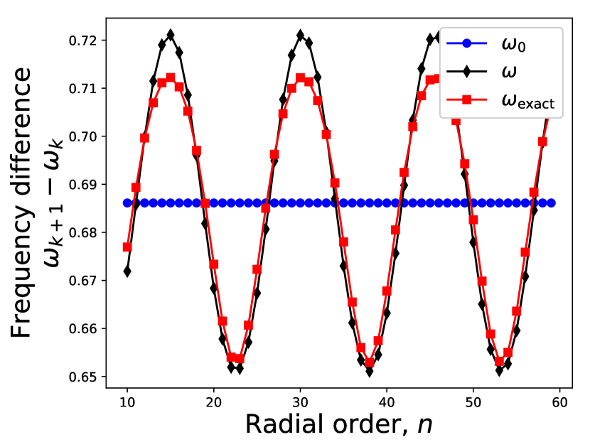
Figure 20: Large frequency separations for various calculations of the frequency: $\omega_{0}$ corresponds to the zeroth order expression (i.e. no perturbations to the sound velocity are included), $\omega$ to the first order approximation, and $\omega_{\mathrm{exact}}$ to exact solutions of the discriminant equations.

Appendix E Wave refraction and reflection

In this section, we recall some of the basic principles behind the Snell-Descartes law including partial wave reflection. A more complete treatment can be found in various textbooks such as Brekhovskikh (1980).

We begin with a simple plane-parallel model using Cartesian coordinates. This can also be thought of as a local approximation to a more complex system. A discontinuity in density is located at $z=0$. The media below and above this discontinuity is assumed to be uniform. Under these conditions, the fluid dynamic equations take on the following expressions:

$$0 = \frac{\delta\rho}{\rho_{0}}+\@vec{\nabla}\cdot\@vec{\xi},$$ (86)

$$\rho_{0}\frac{\partial^{2}\@vec{\xi}}{\partial t^{2}} = -P_{0}\@vec{\nabla}\frac{\delta p}{P_{0}},$$ (87)

$$\frac{\delta p}{P_{0}} = \Gamma_{1}\frac{\delta\rho}{\rho_{0}}.$$ (88)

The interface conditions, as explained in App. A, ensure the continuity of $\frac{\delta p}{P_{0}}$ and $\xi_{z}$. Combining these equations leads to:

$$\frac{\partial^{2}}{\partial t^{2}}\left(\frac{\delta p}{P_{0}}\right)=c_{0}^{2}\Delta\left(\frac{\delta p}{P_{0}}\right).$$ (89)

Because of the partial reflection at the boundary, we cannot consider a plane-parallel wave in isolation but have to include the reflected wave. For the sake of generality, we consider such a combination both above and below the discontinuity. The leads to following generic solution:

$$\left(\frac{\delta p}{P_{0}}\right)^{\pm}=A_{1}^{\pm}\exp(i\@vec{k}_{1}^{\pm}\cdot\@vec{x}+i\omega t)+A_{2}^{\pm}\exp(i\@vec{k}_{2}^{\pm}\cdot\@vec{x}+i\omega t),$$ (90)

where the superscripts ‘$+$’ and ‘$-$’ designate the upper and lower domains, respectively. The standing wave equivalent to the above solution would take on the expression:

$$\left(\frac{\delta p}{P_{0}}\right)^{\pm}=\left[A_{1}^{\pm}\cos(\@vec{k}_{1}^{\pm}\cdot\@vec{x})+A_{2}^{\pm}\cos(\@vec{k}_{2}^{\pm}\cdot\@vec{x})\right]\exp(i\omega t).$$ (91)

The wave vectors take on the following form:

$$\@vec{k}_{1}^{\pm}=\@vec{k}_{\parallel}+k_{z}^{\pm}\@vec{e}_{z},\qquad\@vec{k}_{2}^{\pm}=\@vec{k}_{\parallel}-k_{z}^{\pm}\@vec{e}_{z}.$$ (92)

The horizontal wave vector, $\@vec{k}_{\parallel}$, is preserved between the two domains as a result of the continuity of the horizontal gradient of $\frac{\delta p}{P_{0}}$ at the discontinuity. When combined with the dispersion relation, this leads to Snell-Descartes’ law.

The continuity of $\delta p/P_{0}$ leads to the relation:

$$A_{1}^{+}+A_{2}^{+}=A_{1}^{-}+A_{2}^{-}.$$ (93)

The continuity of $\xi_{z}$ leads to:

$$\frac{A_{1}^{+}-A_{2}^{+}}{\rho_{0}^{+}}=\frac{A_{1}^{-}-A_{2}^{-}}{\rho_{0}^{-}}.$$ (94)

Combining these two equations leads the following matrix relation between the amplitudes:

$$\left[\begin{array}[]{c}A_{1}^{+}\\ A_{2}^{+}\end{array}\right]=\frac{1}{2}\left[\begin{array}[]{cc}1+\eta&1-\eta\\ 1-\eta&1+\eta\end{array}\right]\left[\begin{array}[]{c}A_{1}^{-}\\ A_{2}^{-}\end{array}\right],$$ (95)

where

$$\eta=\frac{\rho_{0}^{+}}{\rho_{0}^{-}}\frac{k_{z}^{-}}{k_{z}^{+}}.$$ (96)

When the wave vector is nearly perpendicular to the discontinuity, that is, $k_{\parallel}\ll k_{z}$, $\eta$ takes on the following approximate expression:

$$\eta\simeq\sqrt{\frac{\rho_{0}^{+}}{\rho_{0}^{-}}}=\frac{c_{0}^{-}}{c_{0}^{+}}.$$ (97)