SiO Outflows as Tracers of Massive Star Formation in Infrared Dark Clouds

Abstract

To study the early phases of massive star formation, we present ALMA observations of SiO(5-4) emission and VLA observations of 6 cm continuum emission towards 32 Infrared Dark Cloud (IRDC) clumps, spatially resolved down to $\lesssim 0.05$ pc. Out of the 32 clumps, we detect SiO emission in 20 clumps, and in 11 of them the SiO emission is relatively strong and likely tracing protostellar outflows. Some SiO outflows are collimated, while others are less ordered. For the six strongest SiO outflows, we estimate basic outflow properties. In our entire sample, where there is SiO emission, we find 1.3 mm continuum and infrared emission nearby, but not vice versa. We build the spectral energy distributions (SEDs) of cores with 1.3 mm continuum emission and fit them with radiative transfer (RT) models. The low luminosities and stellar masses returned by SED fitting suggest these are early stage protostars. We see a slight trend of increasing SiO line luminosity with bolometric luminosity, which suggests more powerful shocks in the vicinity of more massive YSOs. We do not see a clear relation between the SiO luminosity and the evolutionary stage indicated by $L/M$. We conclude that as a protostar approaches a bolometric luminosity of $\sim 10^{2}\>L_{\odot}$, the shocks in the outflow are generally strong enough to form SiO emission. The VLA 6 cm observations toward the 15 clumps with the strongest SiO emission detect emission in four clumps, which is likely shock ionized jets associated with the more massive ones of these protostellar cores.

cont#1 (cont.)#2#3

1 Introduction

Massive stars play a key role in the regulation of galactic environments and galaxy evolution, yet there is no consensus on even the basics of their formation mechanism. Theories range from models based on Core Accretion, i.e., formation from massive self-gravitating cores (e.g., McKee & Tan 2003), to Competitive Accretion, i.e., chaotic clump-fed accretion concurrent with star cluster formation (e.g., Bonnell et al. 2001; Wang et al. 2010), to Protostellar Collisions (e.g., Bonnell et al. 1998; Bally & Zinnecker 2005).

Magneto-centrifugally driven protostellar outflows are thought to be an ubiquitous feature of ongoing formation of all masses of stars (e.g., Arce et al. 2007; Beltrán & de Wit 2016) and are likely to be essential or at least important for removing angular momentum from the accreting gas. Such outflows involving large scale magnetic fields threading the disk (i.e., “disk winds”; e.g., Königl & Pudritz 2000) and/or stellar magnetic fields (i.e., “x-winds”; e.g., Shu et al. 2000) lead to collimated bipolar outflows that can be the most obvious signpost of early star formation activity. Thus studies of the morphologies and kinematics of such outflows can help us understand protostellar activities from inner disk to core envelope scales and beyond. Whether protostellar outflow properties scale smoothly with the mass of the driving protostar will also shed light on how massive star formation differs from low-mass star formation. As one example, radio surveys have found an association of “radio jets”, i.e., collimated radio emission, and molecular outflows that appears to be a common phenomenon in both low-mass (Anglada 1996) and high-mass protostars (Purser et al. 2016; Rosero et al. 2016, 2019b).

With the development of high-resolution, high-sensitivity facilities like ALMA and VLA, more and more observations have been carried out towards massive star-forming regions. While most mm and radio surveys are towards more evolved massive protostars (e.g., Motte et al. 2018; CORE, Beuther et al. 2018; ATOMS, Liu et al. 2020; Rosero et al. 2016; Purser et al. 2016), the earlier stages remain relatively unexplored with only a few surveys being carried out recently (e.g., ASHES, Sanhueza et al. 2019; CORE-extension, Beuther et al. 2021). To study such early stages, we focus on protostars in Infrared Dark Clouds (IRDCs). IRDCs are cold ($T<$20 K), dense ($n_{\rm H}\gtrsim 10^{4}\>{\rm cm}^{-3}$) regions of molecular clouds that are opaque at wavelengths $\sim$10 $\rm\mu m$ or longer and thus appear dark against the diffuse Galactic background emission. They are likely to harbor the earliest stages of star formation (see, e.g., Tan et al. 2014; Sanhueza et al. 2019; Li et al. 2019b).

We have conducted a survey of 32 IRDC clumps with ALMA (see Table 1 in Kong et al. 2017). This high mass surface density sample was selected from 10 IRDCs (A-J) by the mid-infrared (Spitzer-IRAC 8 $\mu$m) extinction (MIREX) mapping methods of Butler & Tan (2009, 2012). The distances range from 2.4 kpc to 5.7 kpc. The first goal of this study was to find massive pre-stellar cores. About 100 such core candidates have been detected via their $\rm N_{2}D^{+}(3-2)$ emission (Kong et al. 2017).

Next, we identified 1.3 mm continuum cores in the 32 clumps (Liu et al. 2018). In total, 107 cores were found with a dendrogram algorithm with a mass range from 0.150 to 178 $M_{\odot}$ assuming a temperature of 20 K.

The ALMA observations are also sensitive to SiO(5-4) emission. SiO is believed to form through sputtering and grain-grain collisions of dust grains (e.g., Schilke et al. 1997; Caselli et al. 1997). Unlike CO, SiO emission does not suffer from confusion with easily excited ambient material. While SiO emission with a narrow velocity range may come from large-scale colliding gas flows (e.g., Jiménez-Serra et al. 2010; Cosentino et al. 2018, 2020), SiO emission with a broad velocity range is considered to be an effective tracer of fast shocks from protostellar outflows. In low-mass protostars, SiO jets are often detected and the detection rate increases with source luminosity (e.g., Podio et al. 2021). Here we use such SiO emission as a tracer of outflows, which are then signposts to help identify and characterize the protostars.

We have also carried out VLA follow-up observations towards our protostar sample to determine the onset of the appearance of radio continuum emission and thus diagnose when the protostars transition from a “radio quiet” to a “radio loud” phase.

The structure of the paper is as follows. In §2 we summarize the ALMA and VLA observations. We present the results of SiO outflows in §3 and 6 cm radio emission in §4. We discuss the implications of the results in §5. We summarize the conclusions in §6.

2 Observations

2.1 ALMA data

We use data from ALMA Cycle 2 project 2013.1.00806.S (PI: Tan), which observed 30 positions in IRDCs on 04-Jan-2015, 10-Apr-2015 and 23-Apr-2015, using 29 12 m antennas in the array. Track 1 with central $v_{\rm LSR}$ = 58 km/s includes clumps A1, A2, A3 ($v_{\rm LSR}\sim$66 km/s), B1, B2 ($v_{\rm LSR}\sim$26 km/s), C2, C3, C4, C5, C6, C7, C8, C9 ($v_{\rm LSR}\sim$79 km/s), E1, E2 ($v_{\rm LSR}\sim$80 km/s) with notations following Butler & Tan (2012) (see Table 1 in Kong et al. 2017 for a list of targets). Track 2 with central $v_{\rm LSR}$ = 66 km/s includes D1, D2 (also contains D4), D3, D5 (also contains D7), D6, D8, D9 ($v_{\rm LSR}\sim$87 km/s), F3, F4 ($v_{\rm LSR}\sim$58 km/s), H1, H2, H3, H4, H5, H6 ($v_{\rm LSR}\sim$44 km/s). In Track 1, J1924-2914 was used as the bandpass calibrator, J1832-1035 was used as the gain calibrator, and Neptune was the flux calibrator. In Track 2, J1751+0939 was used as the bandpass calibrator, J1851+0035 was used as the gain calibrator, and Titan was the flux calibrator. The total observing time including calibration was 2.4 hr. The actual on-source time was $\sim$2-3 min for each pointing.

The spectral set-up included a continuum band centered at 231.55 GHz (LSRK frame) with width 1.875 GHz from 230.615 GHz to 232.490 GHz. At 1.3 mm, the primary beam of ALMA 12m antennas is $\sim 27\arcsec$ (FWHM) and the largest recoverable scale for the array is $\sim 7\arcsec$. The data were processed using NRAO’s Common Astronomy Software Applications (CASA) package (McMullin et al. 2007). For reduction of the data, we used “Briggs” cleaning and set robust = 0.5. The continuum image reaches a 1$\sigma$ rms noise of 0.2 mJy in a synthesized beam of 1.2$\arcsec$ $\times$ 0.8$\arcsec$. The spectral line sensitivity per 0.2 $\rm km\>s^{-1}$ channel is $\sim$0.02 Jy beam^-1 for Track 1 and $\sim$0.03 Jy beam^-1 for Track 2. Other basebands were tuned to observe N₂D⁺(3-2), SiO(5-4), $\rm C^{18}O$ (2-1), DCN(3-2), DCO⁺(3-2) and $\rm CH_{3}OH(5_{1,4}-4_{2,2})$.

2.2 VLA data

The 6 cm (C-band) observations were made towards some of the clumps with strongest SiO in both C configuration and A configuration. The C configuration data taken in 2017 are from project code 17A-371 (PI: Liu) and include A1, A2, A3 in Cloud A (gain calibrator: J1832-1035, positional accuracy 0.01 - 0.15$\arcsec$), B1, B2 in Cloud B (gain calibrator: J1832-1035), C1 (RA: 18:42:46.498, DEC: -4:04:15.964), C2, C4, C5, C6, C9 in Cloud C (gain calibrator: J1832-1035), D1, D8 in Cloud D (gain calibrator: J1832-1035) and H5, H6 in Cloud H (gain calibrator: J1824+1044, positional accuracy $<$ 0.002$\arcsec$). The A configuration data taken in 2018 are from project code 18A-405 (PI: Liu) and include A1, A2, A3 in Cloud A (gain calibrator: J1832-1035), C1, C2, C4, C5, C6, C9 in Cloud C (gain calibrator: J1804+0101, positional accuracy $<$ 0.002$\arcsec$) and H5, H6 in Cloud H (gain calibrator: J1824+1044). 3C286 was used as flux density and bandpass calibrator for all the regions with both configurations. Both sets of data consist of two 2 GHz wide basebands (3 bit samplers) centered at 5.03 and 6.98 GHz, where the first baseband was divided into 16 spectral windows (SPWs), each with a bandwidth of 128 MHz and the second baseband was divided into 15 SPWs with 14 SPWs 128 MHz wide each and 1 SPW 2 MHz wide for the 6.7 GHz methanol maser. The data were recorded in 31 unique SPWs, 30 comprised of 64 channels with each channel being 2 MHz wide and 1 comprised of 512 channels with each channel being 3.906 kHz wide, resulting in a total bandwidth of 3842 MHz (before “flagging”). For sources in Cloud A and C the observations were made alternating on a target source for 9.5 minutes and a phase calibrator for 1 minute, for a total on-source time of 47.5 minutes. For sources in Cloud B, D and H the observations were made alternating on a target source for 8.5 minutes and a phase calibrator for 1 minute, for a total on-source time of 42.5 minutes.

The data were processed using NRAO’s CASA package (McMullin et al. 2007). We used the VLA pipeline CASA v5.1 for the A configuration and pipeline CASA v4.7.2 for the C configuration for calibration. We ran one additional pass of CASA’s flagdata task using the rflag algorithm on each target field to flag low-level interference. For Cloud A, C and H, for which we have data observed with both configurations, we used CASA’s concat task to combine the A configuration and C configuration data giving a factor of 3 times more weight to the A configuration data, allowing us to obtain a more Gaussian-like PSF at a similar resolution as the A-configuration data. We made mosaic images combining all the fields in the same cloud since there was substantial overlap in their primary beams to improve sensitivity and uv-coverage. For Cloud C we used “mosaic” gridder in CASA’s tclean task to jointly deconvolve all 6 fields. The continuum images were made using 29 of the 30 wide-band spectral windows, since one SPW was excluded due to possible contamination by maser emission. All images were deconvolved using the mtmfs mode of CASA’s tclean task and used nterms=2 to model the sources’ frequency dependencies. For Cloud A, B, D, H, we tried different approaches and concluded that the CASA linearmosaic tool gave us the optimal results. Note that mosaics of B and D clouds only include C configuration data. A list of the beam sizes and rms noise levels are shown in Table 1.

Table 1: VLA 6 cm Observations

Source	Configuration	Beam	Continuum	Continuum 3$\sigma$ rms
		Size	Detection	($\mu$Jy beam-1)
A1	A, C	0.659$\arcsec$ $\times$ 0.364$\arcsec$	Y	9.9
A2	A, C	0.659$\arcsec$ $\times$ 0.364$\arcsec$	N	15.0
A3	A, C	0.659$\arcsec$ $\times$ 0.364$\arcsec$	N	17.4
B1	C	4.685$\arcsec$ $\times$ 2.576$\arcsec$	N	18.6
B2	C	4.685$\arcsec$ $\times$ 2.576$\arcsec$	N	20.4
C1	A, C	0.481$\arcsec$ $\times$ 0.396$\arcsec$	N	15.0
C2	A, C	0.481$\arcsec$ $\times$ 0.396$\arcsec$	Y	9.0
C4	A, C	0.481$\arcsec$ $\times$ 0.396$\arcsec$	Y	8.1
C5	A, C	0.481$\arcsec$ $\times$ 0.396$\arcsec$	N	8.7
C6	A, C	0.481$\arcsec$ $\times$ 0.396$\arcsec$	N	12.6
C9	A, C	0.481$\arcsec$ $\times$ 0.396$\arcsec$	Y	13.8
D1	C	3.332$\arcsec$ $\times$ 2.701$\arcsec$	N	20.7
D8	C	3.332$\arcsec$ $\times$ 2.701$\arcsec$	N	25.2
H5	A, C	0.407$\arcsec$ $\times$ 0.326$\arcsec$	N	9.3
H6	A, C	0.407$\arcsec$ $\times$ 0.326$\arcsec$	N	9.0

3 SiO outflows

3.1 SiO detection

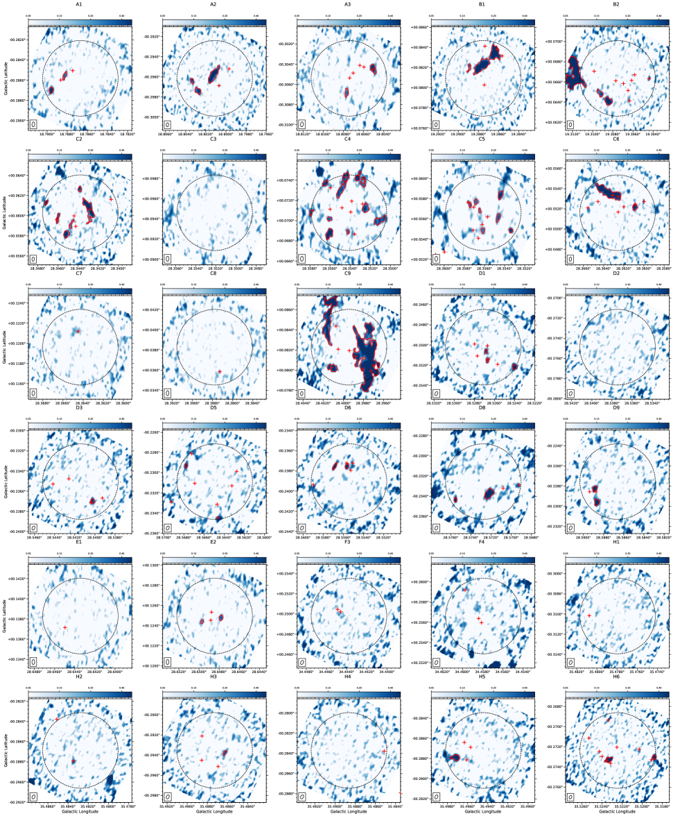
Figure 1: SiO(5-4) integrated intensity maps within $\pm$ 15 km $\rm s^{-1}$ relative to the cloud velocity of the 30 IRDC positions. The red contours show the trunk structures characterized by the dendrogram algorithm. The minimum threshold intensity required to identify a trunk structure is 3 $\sigma$. In the images prior to primary beam correction $\sigma\sim 50\>{\rm mJy\>km\>s}^{-1}\>{\rm beam}^{-1}$ for Clouds A, C, E; $\sigma\sim 40\>{\rm mJy\>km\>s^{-1}\>beam}^{-1}$ for Cloud B; and $\sigma\sim 74\>{\rm mJy\>km\>s^{-1}\>beam}^{-1}$ for Clouds D, F and H. The minimum area is one synthesized beam size. The black plus sign denotes the center of the field. The red plus signs denote the 1.3 mm continuum cores detected in Liu et al. (2018). The dotted circle in each panel denotes the primary beam. The synthesized beam is shown in the bottom left corner of each panel.

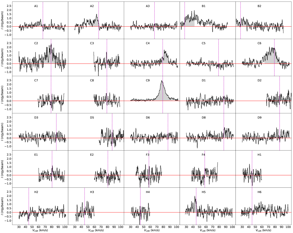
Figure 2: Spectra of SiO(5-4) emission of the 30 IRDC positions averaged within the primary beam. The flux of C9 has been reduced by a scale factor of 0.25 for ease of viewing. The dashed lines denote the estimates of the cloud LSR velocities. The grey area denotes emission within $\pm$15 km $\rm s^{-1}$ relative to the cloud velocity, which is used for identifying structures above 3 $\sigma$ in the integrated intensity maps of SiO(5-4).

Out of the 32 clumps observed, we have detected SiO(5-4) emission in 20 sources: A1, A2, A3, B1, B2, C2, C4, C5, C6, C9, D1, D3, D5, D6, D8, D9, E2, H3, H5, H6. We define a detection of SiO(5-4) emission with two methods. Method 1 is if there are at least 3 consecutive pixels with the peak emission greater than $3\sigma$ noise level in their spectra and the projected area of such pixels is larger than one beam size. Method 2 is if the integrated intensity of SiO(5-4) within $\pm$15 km $\rm s^{-1}$ relative to the cloud velocity is higher than the $3\sigma$ noise level and the area of such pixels is larger than one beam size (see Figure 1). We only consider emission inside the primary beam (except B2, see §3.2). When applying Method 2, the emission features were identified by the dendrogram algorithm (Rosolowsky et al. 2008), which is a code for identifying hierarchical structures. We set the minimum threshold intensity required to identify a parent tree structure (trunk) to be 3$\sigma$ and a minimum area of the synthesized beam size. We use the images prior to primary beam correction to identify cores. We use astrodendro, a python package to compute dendrogram statistics. Only A2, B1, B2, C2, C4, C5, C6, C9 are reported detection with Method 1. More detections are made with Method 2. This indicates the sources detected with Method 2, but not Method 1, generally have weak emission in each channel and their signal only starts to show up after integration. The spectra of the 30 IRDC positions averaged within the primary beam are shown in Figure 2. These figures also show the estimated systemic velocity of each cloud, adopted from Kong et al. (2017).

To identify the protostellar sources that are responsible for the generation of the SiO(5-4) emission, we search for 1.3 mm emission peaks that are in the vicinity. Although there is at least one continuum peak in every clump with SiO detection, it is ambiguous in many cases to tell the association of SiO and continuum peaks based only on their spatial distributions.

We are more confident about the protostellar nature of a continuum peak if it is associated with a dense gas tracer $\rm C^{18}O$(2-1), DCN(3-2) or DCO⁺(3-2). For each 1.3 mm continuum source identified in Liu et al. (2018), we define a 3$\arcsec$ $\times$ 3$\arcsec$ region centered at the continuum peak as the “core region” and derive the spectrum of each dense gas tracer within the core region. If there are more than 3 channels with signal above 2$\sigma$ noise level, and the peak channel as well as its neighboring channels have signal above a 2$\sigma$ noise level, then we consider there is detection of that line associated with the continuum core. We record the peak velocity of each line and take the mean value as the systemic velocity of the core. Generally $\rm C^{18}O$(2-1) is the most common tracer. DCN(3-2) and DCO⁺(3-2) can be relatively weak. The SiO detections and the association with 1.3 mm continuum emission peaks and dense gas tracers are summarized in Table 2.

Table 2: Integrated Flux Densities

Source	$d$	$L_{\rm SiO,total}$	SiO Detection				Plausible Driving Protostar										Photometry and SED Fitting
	(kpc)	(Jy km s-1 pc2)	No.	$l$	$b$	$S_{\nu}$	mm Peak	$l$	$b$	$M_{c,\rm raw}$	DCN	DCO+	C18O	CH3OH	N2D+	velocity	$l_{\rm ap}$	$b_{\rm ap}$	$R_{\rm ap}$	$L_{\rm bol}$
				($\arcdeg$)	($\arcdeg$)	(Jy km s-1)		($\arcdeg$)	($\arcdeg$)	($M_{\odot}$)						(km s$-1$)	($\arcdeg$)	($\arcdeg$)	($\arcsec$)	$L_{\odot}$
A1	4.8	2.733$\times 10^{8}$	1	18.78830	-0.28567	0.328	A1c2	18.78864	-0.28598	23.0	N	N	Y	N	Y	64.2	18.78897	-0.28477	16	5.771$\times 10^{2}$
			2	18.78963	-0.28711	0.616	A1c2	18.78864	-0.28598	23.0	N	N	Y	N	Y	64.2
A2	4.8	1.504e+09	1	18.80129	-0.29592	3.826	A2c2	18.80070	-0.29687	3.49	Y	Y	Y	N	N	55.2	18.80177	-0.29591	16	4.132$\times 10^{2}$
			2	18.80340	-0.29650	0.444
			3	18.80281	-0.29750	0.926
A3	4.8	3.706$\times 10^{8}$	1	18.80510	-0.30455	0.938	A3c3	18.80509	-0.30452	16.5	N	Y	Y	N	N	66.0	18.80612	-0.30392	16	4.194$\times 10^{2}$
			2	18.80772	-0.30693	0.342	A3c5	18.80738	-0.30536	0.971	N	Y	Y	N	Y	65.3
B1	2.4	9.686$\times 10^{8}$	1	19.28645	0.08332	5.959	B1c2	19.28614	0.08382	4.18	Y	Y	Y	N	N	26.8	19.28618	0.08371	11	8.106$\times 10^{1}$
			2	19.28777	0.08203	7.061	B1c2	19.28614	0.08382	4.18	Y	Y	Y	N	N	26.8
			3	19.28898	0.08192	0.361	B1c2	19.28614	0.08382	4.18	Y	Y	Y	N	N	26.8
B2	2.4	1.050e+10	1	19.31186	0.06678	35.549	B2c9	19.31166	0.06737	14.4	Y	N	Y	Y	N	26.0	19.31172	0.06726	15	2.976$\times 10^{2}$
							B2c10	19.31149	0.06633	2.31	Y	N	Y	Y	N	26.4
			2	19.30930	0.06477	0.700
			3	19.30850	0.06399	2.048
C2	5.0	2.350e+09	1	28.34389	0.06251	0.457											28.34574	0.06053	16	9.451$\times 10^{2}$
			2	28.34721	0.06116	0.439
			3	28.34298	0.06052	4.407	C2c2	28.34284	0.06061	48.5	Y	Y	Y	N	N	79.2
			4	28.34607	0.05962	0.624	C2c4	28.34610	0.05963	33.1	Y	Y	Y	Y	N	83.7
			5	28.34473	0.05901	0.372
			6	28.34523	0.05804	1.181
C4	5.0	2.899e+09	1	28.35328	0.07419	0.923											28.35456	0.07170	13	2.103$\times 10^{2}$
			2	28.35274	0.07370	0.593
			3	28.35651	0.07358	0.523	C4c2	28.35596	0.07326	9.65	Y	N	N	Y	N	94.8
			4	28.35475	0.07349	2.566	C4c1	28.35446	0.07388	16.8	N	N	Y	Y	N	83.1
			5	28.35254	0.07112	0.952	C4c4	28.35276	0.07166	6.87	N	N	Y	Y	N	81.3
			6	28.35791	0.07067	0.336
			7	28.35610	0.07006	0.284	C4c6	28.35599	0.07114	0.509
			8	28.35110	0.06992	1.303
			9	28.35427	0.06879	0.196	C4c8	28.35356	0.06867	3.10
			10	28.35612	0.06858	1.552
C5	5.0	7.864$\times 10^{8}$	1	28.35447	0.05825	0.768											28.35620	0.05782	15	2.618$\times 10^{2}$
			2	28.35690	0.05758	0.276	C5c2	28.35705	0.05718	1.13
			3	28.35751	0.05732	0.247	C5c1	28.35757	0.05759	1.68
			4	28.35653	0.05670	0.150
			5	28.35470	0.05602	0.492
			6	28.35621	0.05475	0.247
			7	28.35344	0.05475	0.323	C5c4	28.35622	0.05544	2.88
C6	5.0	3.511e+09	1	28.36350	0.05346	10.276	C6c1	28.36310	0.05336	9.30	N	N	Y	Y	Y	80.0	28.36315	0.05323	15	4.484$\times 10^{2}$
							C6c2	28.36258	0.05322	3.01	N	N	Y	Y	Y	81.0
			3	28.36096	0.05206	0.901	C6c5	28.36085	0.05246	8.77	N	N	Y	N	N	79.4
C9	5.0	1.981e+10	1	28.40145	0.08545	13.221											28.39708	0.08034	10	6.284$\times 10^{3}$
			2	28.39759	0.08080	63.052	C9c5	28.39701	0.08045	178	Y	Y	Y	Y	N	77.0
							C9c7	28.39806	0.08011	25.6	Y	Y	Y	Y	N	78.5
							C9c8	28.39726	0.07993	39.1	Y	Y	Y	Y	N	80.0
			3	28.40113	0.08011	1.883	C9c6	28.40118	0.08028	13.9	N	N	N	N	N
D1	5.7	5.574$\times 10^{8}$	1	28.52691	-0.25075	0.324											28.52727	-0.25093	15	2.957$\times 10^{2}$
			2	28.52675	-0.25162	0.288	D1c4	28.52666	-0.25146	5.34	N	Y	Y	N	Y	86.6
			3	28.52409	-0.25228	0.754
D3	5.7	2.144$\times 10^{8}$	1	28.54031	-0.23711	0.525	D3c4	28.54037	-0.23710	1.01	Y	Y	N	Y	N	88.1	28.54167	-0.23443	15	4.533$\times 10^{2}$
D5	5.7	1.531$\times 10^{8}$	1	28.56784	-0.22944	0.375	D5c1	28.56724	-0.22810	2.61	N	N	Y	N	N	87.4	28.56469	-0.23413	11	3.726$\times 10^{2}$
D6	5.7	4.713$\times 10^{8}$	1	28.55691	-0.23766	0.632											28.55816	-0.23847	15	2.758$\times 10^{2}$
			2	28.55571	-0.23766	0.522	D6c1	28.55565	-0.23721	8.65	Y	Y	Y	N	N	83.0
D8	5.7	1.413e+09	1	28.57227	-0.23388	2.960	D8c2	28.57080	-0.23321	0.843	N	N	Y	N	N	88.9	28.56960	-0.23314	11	2.330$\times 10^{2}$
			2	28.57559	-0.23445	0.500
D9	5.7	8.494$\times 10^{8}$	1	28.58892	-0.22837	0.894	D9c2	28.58877	-0.22855	28.3	N	Y	Y	N	N	86.3	28.58980	-0.22818	12	1.653$\times 10^{2}$
			2	28.58871	-0.22972	1.187	D9c2	28.58877	-0.22855	28.3	N	Y	Y	N	N	86.3
E1	5.1		0	-	-	-	-	-	-	-	-	-	-	-	-	-	28.64497	0.13900	15	1.743$\times 10^{2}$
E2	5.1	1.487$\times 10^{8}$	1	28.64787	0.12465	0.312	E2c2	28.64883	0.12454	3.72	N	N	Y	Y	N	78.7	28.64893	0.12560	15	2.083$\times 10^{2}$
			2	28.64975	0.12427	0.143	E2c2	28.64883	0.12454	3.72	N	N	Y	Y	N	78.7
F3	3.7		0	-	-	-	-	-	-	-	-	-	-	-	-	-	34.44478	0.25019	6	2.398$\times 10^{1}$
F4	3.7		0	-	-	-	-	-	-	-	-	-	-	-	-	-	34.45981	0.25909	15	8.865$\times 10^{1}$
H1	2.9		0	-	-	-	-	-	-	-	-	-	-	-	-	-	35.48076	-0.31016	15	8.717$\times 10^{1}$
H2	2.9		0	-	-	-	-	-	-	-	-	-	-	-	-	-	35.48380	-0.28637	10	3.910$\times 10^{1}$
H3	2.9	3.077$\times 10^{7}$	1	35.48633	-0.29391	0.291	H3c3	35.48693	-0.29513	5.86	N	Y	N	N	N	43.6	35.48765	-0.29326	11	3.370$\times 10^{1}$
H4	2.9		0	-	-	-	-	-	-	-	-	-	-	-	-	-	35.48504	-0.28344	10	6.373$\times 10^{1}$
H5	2.9	1.584$\times 10^{8}$	1	35.49724	-0.28803	1.499	H5c3	35.49611	-0.28813	6.39	N	N	Y	N	N	44.7	35.49653	-0.28683	11	5.030$\times 10^{1}$
H6	2.9	1.864$\times 10^{8}$	1	35.51886	-0.27317	0.647	H6c7	35.51908	-0.27330	0.363	N	Y	Y	N	N	47.5	35.52357	-0.27351	12	8.366$\times 10^{1}$
			2	35.52338	-0.27343	1.764	H6c8	35.52352	-0.27337	2.53	N	Y	Y	N	Y	45.2

3.2 Strong SiO Sources

There are 6 clumps (B1, B2, C2, C6, C9, H6) in which the peak of the SiO integrated intensity is stronger than 10$\sigma$, as well as being clearly associated with identified continuum sources. They are likely protostars driving SiO outflows. In this section we present the outflow morphologies, outflow kinematics and SED fitting results of the 6 protostar candidates which show strongest SiO outflow emission. As described in the previous sub-section, the radial velocity of the protostar is estimated from the dense gas tracers $\rm C^{18}O$(2-1), DCN(3-2) and DCO⁺(3-2). Once the source velocity is defined, the velocity range of the SiO(5-4) emission for the source is determined by looking at the SiO spectra pixel by pixel in the outflow area.

3.2.1 Morphology and Kinematics

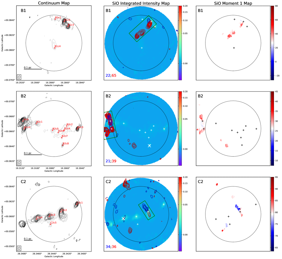
Figure 3: Left Column: 1.3 mm continuum maps. Contour levels are evenly spaced logarithmically, corresponding to 0.800, 1.15, 1.65, 2.36, 3.39, 4.86, 6.98, 10.0, 14.4, 20.6, 29.6, 42.5, 60.9, 87.4, 125, 180 $\rm mJy\ beam^{-1}$. The rms noise level in each image is $\sim\ 0.2\ \rm mJy\ beam^{-1}$, except for C9 that is dynamic range dominated and has an rms noise level of $\sim\ 0.6\ \rm mJy\ beam^{-1}$. The contours below 2 $\rm mJy\ beam^{-1}$ are dotted. Note, here we only show emission above the 3 $sigma$ noise level. The small red plus signs denote the peaks of the dendrogram-identified continuum cores (Liu et al. 2018). The large black plus sign denotes the center of the observation. The dashed circle shows the FWHM of the primary beam. A scale bar and beam size are shown in the lower left corner. Middle Column: Integrated intensity maps of SiO(5-4) emission (contours) over 1.3 mm continuum emission (color scale in Jy beam^-1). Contour levels start at 5$\sigma$ in steps of 4$\sigma$ noise level of the integrated intensity. The 1$\sigma$ noise values of the blue- and red-shifted outflows are written in the left corner in unit of mJy beam^-1 s^-1. The velocity ranges are listed in Table 3. The green rectangles denote the apertures for deriving the averaged spectra and averaged PV diagrams. The small white plus signs denote the peaks of the dendrogram-identified continuum cores (Liu et al. 2018). White X signs denote water masers detected by Wang et al. (2016). The dashed circle shows the primary beam. Right Column: Intensity weighted velocity (first moment) maps of SiO(5-4) emission (color scale in km s^-1). Note we only use pixels with emission stronger than 3$\sigma$ noise level for H6 and 4$\sigma$ noise level for the other sources. The small black plus signs denote the peaks of the dendrogram-identified continuum cores (Liu et al. 2018). The dashed circle shows the primary beam.

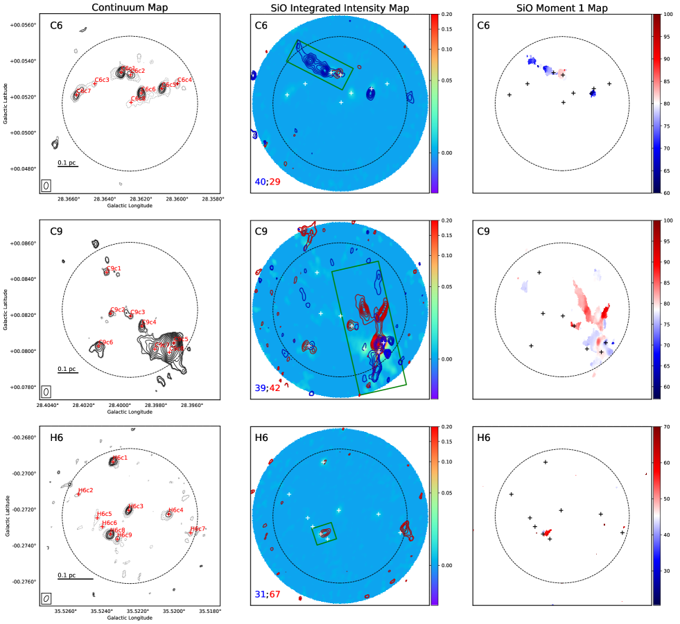
Figure 3: (cont.)

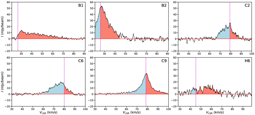
Figure 4: Averaged SiO(5-4) spectra extracted from the defined rectangular aperture of each source (see Figure 3). The dashed line denotes the systemic velocity of the 1.3 mm continuum sources. The blue and red areas denote the velocity range used to derive the blue- and red-shifted outflows, respectively.

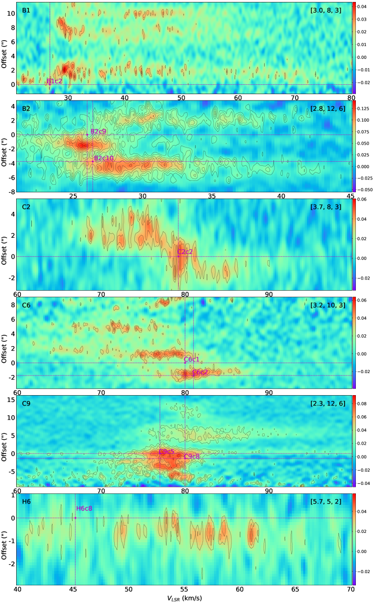
Figure 5: Averaged position-velocity diagram of SiO(5-4) emission along the long axis of the rectangles shown in Figure 3, i.e., the outflow axes. The offset from top to bottom corresponds to the offset from the reference position along the axis from east to west. The reference position is where the continuum peak is located. Other continuum peaks in the rectangle are also shown if any. Color scale is in Jy beam^-1. Contour level information is given in upper right: 1 $\sigma$ noise level in mJy beam^-1; lowest contour level in number of $\sigma$; then step size between each contour in number of $\sigma$.

We show the continuum maps, integrated intensity maps of SiO(5-4) and velocity maps of SiO(5-4) of these sources in Figure 3. The names of the continuum cores are the same with those in Liu et al. (2018). By checking the channel maps, we find that the SiO emission with very low velocity ($\rm\lesssim 3km~{}\rm s^{-1}$) also follows the shape of the outflow. Thus in our fiducial method we do not consider ambient gas as one would do with CO outflows. The averaged spectra of SiO(5-4), extracted from the defined rectangular apertures around each source, are shown in Figure  4. The velocity span of the SiO emission from these sources is $\sim$30 km $\rm s^{-1}$. The averaged position-velocity (PV) diagrams in the rectangular apertures along the outflow axes are shown in Figure 5. We can see there is large velocity dispersion at a certain position in all the sources.

Overall, some outflows appear quite collimated, like C2 and C6, while others are less ordered, like C9. The morphologies and kinematics of the six sources are discussed individually below.

Source B1: Since the spectral set-up only starts at 21 $\rm km\ s^{-1}$, we may miss some emission from blue-shifted velocities. The velocity range of SiO emission is $\sim$ 50 $\rm km\ s^{-1}$. As shown in Figure 3, the red-shifted component consists of three peaks. We do not see any more emission beyond the current displayed area. However, there may be more blue-shifted emission emerging to the west of the view and in that case the outflow axis would be oriented NW-SE. Otherwise, if the outflow axis is oriented N-S, then the origin of the two red-shifted SiO peaks in the east becomes less clear.

Source B2: There is very strong SiO emission located at the eastern edge of the primary beam. We used the same method in Liu et al. (2018) to identify continuum cores in the outflow region outside of the primary beam. Even though the noise is higher than inside the primary beam, we were still able to identify two cores B2c9 and B2c10. B2c9 has a mass of 14.4 $M_{\odot}$ and a mass surface density of 3.14 g cm^-2 (assuming 20 K dust temperature). Similarly, B2c10 has a mass of 2.31 $M_{\odot}$ and a mass surface density of 1.32 g cm^-2. The velocity range of SiO emission is $\sim$24 $\rm km\ s^{-1}$. Like B1, given the spectral setting we may only see part of the blue-shifted component. The outflow does not reveal a clear bipolar structure and the blue lobes and red lobes overlap as shown in Figure 3. There is also some red-shifted emission within the primary beam which may be connected to the eastern source(s).

Source C2: The 1.3 mm continuum image reveals five peaks. The velocity range of the SiO emission is $\sim$30 $\rm km\ s^{-1}$. The outflow is highly symmetric and highly collimated with a half-opening angle of about 23$\arcdeg$, as shown in Figure 3. Zhang et al. (2015) also observed this clump (G28.34 P1) via 1.3 mm continuum and multiple molecular lines including CO(2-1) and SiO(5-4) with a higher sensitivity, which shows similar results. They determined sub-fragmentation in the 1.3 mm continuum cores with 2D Gaussian fitting. From Figure 5 we can see C2 shows a “Hubble-law” velocity structure (e.g., Lada & Fich, 1996) and similar to the expectation of a single bow shock (Lee et al. 2000), in which the highest velocity appears at the tip followed by a low-velocity “wake” or “bow wing” and the velocity dispersion decreases significantly in the post shocked region closer to the protostar. Arc-like PV structures, similar to those seen in Fig. 5, have been seen in pulsed jet simulations (e.g., Stone & Norman 1993; Lee & Sahai 2004), indicating that this mechanism may be operating here.

Source C6: The velocity range of the SiO emission is about 30 $\rm km\ s^{-1}$. As shown in Figure 3, the two lobes are very asymmetric with the blue lobe extending much further and exhibiting higher velocities (see Figure 5). Similar asymmetry is also revealed in the CO(2-1) outflow, where there is strong blue-shifted emission but little red-shifted emission (Kong et al. 2019). It may be due to an inhomogeneous ambient cloud environment, which is denser in the south, or due to intrinsically variable jets. The blue-shifted outflow is highly collimated, consists of a chain of knots and also has a small wiggle, which resembles the SiO jets revealed in the HH 212 low-mass protostellar system (Lee et al. 2015), the V380 Ori NE region (Choi et al. 2017), and the CO outflow in Serpens South (Plunkett et al. 2015). The knotty feature suggests an episodic ejection mechanism (e.g., Qiu & Zhang 2009; Plunkett et al. 2015; Chen et al. 2016) or alternatively oblique shocks (Reipurth 1992; Guilloteau et al. 1992). The wiggle may be caused by jet precession (e.g., Choi et al. 2017) or instability in a magnetized jet (e.g., Lee et al. 2015). Since we do not see symmetric features in the red-shifted outflow, the orbiting source jet model of a protobinary (e.g., Lee et al. 2010) is not favored, though it is still possible if there is very dense ambient gas located where the red-shifted outflow should be. The PV diagram (see Figure 5) is similar to the SiO jet in H212 (Codella et al. 2007, see their Figure 2 Left). They suggested that the SiO lobes include a narrower and faster jet-like component distinct from the swept-up cavity and the high-velocity SiO is probably tracing the base of the large-scale molecular jet. The velocity structures look like “Hubble wedges” (Arce & Goodman 2001). Recent theoretical models of episodic protostellar outflows (e.g., Federrath et al. 2014; Offner & Arce 2014; Offner & Chaban 2017; Rohde et al. 2019) have been built to reproduce such features. A separate blue-shifted emission feature seems to be driven by the continuum core C6c5, which is associated with a CO(2-1) outflow (Kong et al. 2019). However, the systemic velocity of C6c5 cannot be determined accurately due to the weak emission of its dense gas tracers.

Figure 6: Integrated intensity map in C9 of: (a) $\rm DCO^{+}$(3-2), $\sigma$ = 19.8 mJy ${\rm beam^{-1}}$ km $\rm s^{-1}$; (b) DCN(3-2), $\sigma$ = 19.8 mJy ${\rm beam^{-1}}$ km $\rm s^{-1}$; (c) $\rm C^{18}O$(2-1), $\sigma$ = 35.3 mJy ${\rm beam^{-1}}$ km $\rm s^{-1}$; (d) $\rm CH_{3}OH(5_{1,4}-4_{2,2})$, $\sigma$ = 19.8 mJy ${\rm beam^{-1}}$ km $\rm s^{-1}$. All of these are integrated within $\pm$ 5 km $\rm s^{-1}$ respect to the cloud velocity. Contour levels start at 5$\sigma$ in steps of 4$\sigma$. The pink contours denote the SiO(5-4) emission of all the 360 velocity channels from 30 km $\rm s^{-1}$ to 102 km $\rm s^{-1}$, starting at 380 mJy ${\rm beam^{-1}}$ km $\rm s^{-1}$ in steps of 304 mJy ${\rm beam^{-1}}$ km $\rm s^{-1}$. The small white plus signs denote the positions of the continuum peaks. The large black plus sign denotes the center of view. The dashed circle shows the primary beam. A scale bar and beam size are shown in the lower left corner.

Figure 7: C9 SiO velocity components. (a) Integrated intensity maps of SiO(5-4) emission with low velocity components over continuum emission. Blue contours show emission from 67.0 $\rm km\ s^{-1}$ to 78.5 $\rm km\ s^{-1}$. Red contours show emission from 78.5 $\rm km\ s^{-1}$ to 90.0 $\rm km\ s^{-1}$. Contour levels start at 5$\sigma$ in steps of 4$\sigma$ with with $\sigma$ = 30.5 mJy ${\rm beam^{-1}}$ km $\rm s^{-1}$ for the red-shifted component and $\sigma$ = 30.7 mJy ${\rm beam^{-1}}$ km $\rm s^{-1}$ for the blue-shifted component. The small white plus signs denote the positions of the continuum peaks. The large black plus sign denotes the center of view. The dashed circle shows the primary beam. A scale bar and beam size are shown in the lower left corner. (b) The same as (a), but with high velocity components. Blue contours show emission from 60.0 $\rm km\ s^{-1}$ to 67.0 $\rm km\ s^{-1}$. Red contours show emission from 90.0 $\rm km\ s^{-1}$ to 100 $\rm km\ s^{-1}$. Contour levels start at 5$\sigma$ in steps of 4$\sigma$ with $\sigma$ = 28.6 mJy ${\rm beam^{-1}}$ km $\rm s^{-1}$ for the red-shifted component and $\sigma$ = 24.0 mJy ${\rm beam^{-1}}$ km $\rm s^{-1}$ for the blue-shifted component.

Source C9: The 1.3 mm continuum emission reveals 3 cores in the main outflow area as shown in Figure 3. The brightest core, C9c5, has a peak intensity as high as 197 mJy beam^-1, while the second brightest core, C9c8, to its south has a peak intensity of 85.3 mJy beam^-1. The systemic velocities of C9c5 and C9c8 are listed in Table 2. At the position of continuum core C9c7, the peak velocity of DCN is $\sim$80.0 $\rm km\ s^{-1}$ and the peak velocity of $\rm DCO^{+}$ is $\sim$79.6 $\rm km\ s^{-1}$, while that of $\rm C^{18}O$ is $\sim$75.9 $\rm km\ s^{-1}$. The systemic velocity of C9c4 and C9c6 cannot be determined accurately due to their weak emission in dense gas tracers. The velocity range of the SiO emission is about 40 $\rm km\ s^{-1}$. Figure 6 shows the emission from the dense gas tracers $\rm DCO^{+}$, DCN, $\rm C^{18}O$ and the hot gas tracer $\rm CH_{3}OH$. Their peaks essentially overlap with the continuum peaks. DCN and $\rm CH_{3}OH$ also show extended structures associated with the SiO outflows, while $\rm C^{18}O$ shows additional emission elsewhere. The disordered and asymmetric morphology of the SiO outflows is probably due to the crowded nature of the core region. Several velocity components are revealed from the PV diagram in Figure 5, with a hint of “Hubble wedge”. The most extended red-shifted emission lies mostly in the north and the most extended blue-shifted emission in the south. The morphology could be a result of a combination of the extended outflows from both C9c5 and C9c8. We further display the outflows in low-velocity ($<$ 10 $\rm km\ s^{-1}$ with respect to the systemic velocity) channels and high-velocity ($>$ 10 $\rm km\ s^{-1}$ with respect to the systemic velocity) channels in Figure 7. Together with further investigation in the channel map (not shown here), it is more likely that the two farthest high-velocity red-shifted components revealed in Figure 7(b) come from two distinctive outflows rather than consisting of one outflow cavity wall. In addition to the most extended north-south outflows, there seem to be three other smaller scale outflows from Figure 7(b). One has its blue- and red-shifted components overlapping at C9c5 and is probably driven by this source. The second one has its blue-shifted component to the west of C9c5 and red-shifted components to the east of C9c5, and these features are likely also driven by C9c5. The third one has its blue-shifted component to the southwest of C9c5. From the spacial distribution, this outflow could be driven by either C9c5 or C9c8, and its red-shifted component either lies also to the east of C9c5 or extends further. It is possible that there are more unresolved protostars other than C9c5 and C9c8 in the region that drive the multiple outflows, which would indicate a protobinary or multiple system within our resolution limit of 5000 AU and that they each drive an outflow of a different direction. Another possibility is that the outflow orientation may change over time as reported in other protostars (e.g., Cunningham et al. 2009; Plambeck et al. 2009; Principe et al. 2018; Goddi et al. 2018; Brogan et al. 2018). Nevertheless, the outflows associated with C9c6 and C9c4 are quite clear and relatively separate.

Source H6: The blue-shifted emission is quite weak in this source as shown in Figure 3. This may be partly due to missing blue-shifted channels in our spectral setup. The velocity range of the SiO outflow is about 30 $\rm km\ s^{-1}$.

3.2.2 Outflow Mass and Energetics

Following the method of Goldsmith & Langer (1999) with an assumption of optically thin thermal SiO(5-4) emission in local thermodynamic equilibrium (LTE), we calculate the mass of the SiO(5-4) outflows using

$$N_{u}=\frac{4\pi}{hcA_{\rm ul}}\int(S_{\nu}/\Omega)dv,$$ (1)

$$N_{\rm tot}=N_{u}\frac{U(T_{\rm ex})}{g_{u}}e^{\frac{E_{u}}{kT_{\rm ex}}},$$ (2)

$$M_{\rm out}=N_{\rm tot}\left[\frac{\rm H_{2}}{\rm SiO}\right]\mu_{g}m_{\rm H_{2}}D^{2},$$ (3)

where $S_{\nu}/\Omega$ is the SiO intensity at frequency $\nu$, $D$ is the source distance, $\mu_{g}\ =\ 1.36$ is the mean atomic weight and $m_{\rm H_{2}}$ is the mass of hydrogen molecule. We adopt an excitation temperature of 18 K and a ratio [H₂]/[SiO] of $10^{9}$, which are the typical values of IRDC protostellar sources in the survey of Sanhueza et al. (2012). The momentum and energy of the outflow are then derived following

$$P_{\rm out}=\sum M_{\rm out}(\Delta v)\Delta v$$ (4)

and

$$E_{\rm out}=\frac{1}{2}\sum M_{\rm out}(\Delta v)\Delta v^{2},$$ (5)

where $\Delta v$ denotes the outflow velocity relative to $v_{\rm cloud}$.

Table 3: Estimated Physical Parameters for SiO Outflows

Source	$v_{\rm sys}$	$v_{\rm blue}$	$M_{\rm out}^{\rm blue}$	$P_{\rm out}^{\rm blue}$	$L_{\rm flow}^{\rm blue}$	$t_{\rm dyn}^{\rm blue}$	$v_{\rm red}$	$M_{\rm out}^{\rm red}$	$P_{\rm out}^{\rm red}$	$L_{\rm flow}^{\rm red}$	$t_{\rm dyn}^{\rm red}$	$M_{\rm out}$	$P_{\rm out}$	$E_{\rm out}$	$\dot{M}_{\rm out}$	$\dot{P}_{\rm out}$
	$(\rm km\ s^{-1})$	$(\rm km\ s^{-1})$	$(M_{\odot})$	$(M_{\odot}$	(pc)	$(10^{3}$	$(\rm km\ s^{-1})$	$(M_{\odot})$	$(M_{\odot}$	(pc)	$(10^{3}$	$(M_{\odot})$	$(M_{\odot}$	$(10^{43}$	$(10^{-4}\ M_{\odot}$	$(10^{-4}\ M_{\odot}$
				$\rm km\ s^{-1})$		$\rm yr)$			$\rm km\ s^{-1})$		$\rm yr)$		$\rm km\ s^{-1})$	$\rm erg)$	$\rm yr^{-1})$	$\rm km\ s^{-1}yr^{-1})$
B1	26.8	21.0 $-$ 26.8	0.011	0.031	0.033	11.75 (8.10)	26.8 $-$ 80.0	0.192	2.703	0.131	9.10 (5.13)	0.204	2.735	33.738	0.221	5.310
	26.8	21.0 $-$ 26.8	0.011	0.031	0.033	5.59	26.8 $-$ 80.0	0.192	2.703	0.131	2.40	0.204	2.735	33.738	0.822	11.312
	26.8	21.0 $-$ 23.8	0.006	0.026	0.033	7.54 (7.26)	29.8 $-$ 80.0	0.174	2.292	0.131	9.70 (5.50)	0.180	2.318	26.672	0.187	4.202
	26.8	21.0 $-$ 23.8	0.006	0.026	0.033	5.59	29.8 $-$ 80.0	0.174	2.292	0.131	2.40	0.180	2.318	26.672	0.735	9.589
B2	26.2	21.0 $-$ 26.2	0.138	0.294	0.079	35.98 (24.06)	26.2 $-$ 45.0	0.384	1.531	0.150	36.79 (23.00)	0.522	1.825	5.354	0.143	0.788
	26.2	21.0 $-$ 26.2	0.138	0.294	0.079	14.77	26.2 $-$ 45.0	0.384	1.531	0.150	7.81	0.522	1.825	5.354	0.585	2.160
	26.2	21.0 $-$ 23.2	0.044	0.177	0.079	19.29 (18.78)	29.2 $-$ 45.0	0.267	0.956	0.150	41.00 (28.40)	0.311	1.133	2.831	0.088	0.431
	26.2	21.0 $-$ 23.2	0.044	0.177	0.079	14.77	29.2 $-$ 45.0	0.267	0.956	0.150	7.81	0.311	1.133	2.831	0.372	1.344
C2	79.2	65.0 $-$ 79.2	0.225	1.155	0.121	22.97 (15.74)	79.2 $-$ 95.0	0.145	1.431	0.081	8.06 (7.03)	0.370	2.587	12.441	0.278	2.771
	79.2	65.0 $-$ 79.2	0.225	1.155	0.121	8.31	79.2 $-$ 95.0	0.145	1.431	0.081	5.04	0.370	2.587	12.441	0.558	4.230
	79.2	65.0 $-$ 76.2	0.154	1.063	0.121	17.15 (14.79)	82.2 $-$ 95.0	0.079	0.797	0.081	7.87 (7.11)	0.233	1.860	8.705	0.190	1.839
	79.2	65.0 $-$ 76.2	0.154	1.063	0.121	8.31	82.2 $-$ 95.0	0.079	0.797	0.081	5.04	0.233	1.860	8.705	0.342	2.860
C6	80.0	60.0 $-$ 80.0	0.571	4.354	0.212	27.20 (18.50)	80.0 $-$ 90.0	0.179	2.953	0.079	4.67 (4.55)	0.750	7.307	49.392	0.593	8.840
	80.0	60.0 $-$ 80.0	0.571	4.354	0.212	10.37	80.0 $-$ 90.0	0.179	2.953	0.079	7.70	0.750	7.307	49.392	0.783	8.032
	80.0	60.0 $-$ 77.0	0.442	4.172	0.212	21.99 (17.85)	83.0 $-$ 90.0	0.092	1.586	0.079	4.45 (4.39)	0.534	5.758	38.150	0.407	5.950
	80.0	60.0 $-$ 77.0	0.442	4.172	0.212	10.37	83.0 $-$ 90.0	0.092	1.586	0.079	7.70	0.534	5.758	38.150	0.545	6.082
C9	78.5	60.0 $-$ 78.5	1.942	10.621	0.203	36.36 (20.25)	78.5 $-$ 100.0	2.256	28.378	0.392	30.48 (25.87)	4.197	38.999	262.490	1.274	16.214
	78.5	60.0 $-$ 78.5	1.942	10.621	0.203	10.75	78.5 $-$ 100.0	2.256	28.378	0.392	17.84	4.197	38.999	262.490	3.071	25.790
	78.5	60.0 $-$ 75.5	1.123	9.489	0.203	23.53 (18.48)	81.5 $-$ 100.0	1.360	16.752	0.392	31.14 (26.44)	2.483	26.241	172.524	0.914	11.469
	78.5	60.0 $-$ 75.5	1.123	9.489	0.203	10.75	81.5 $-$ 100.0	1.360	16.752	0.392	17.84	2.483	26.241	172.524	1.807	18.219
H6	45.2	40.0 $-$ 45.2	0.005	0.011	0.011	5.15 (3.77)	45.2 $-$ 70.0	0.025	0.176	0.039	5.34 (3.67)	0.030	0.187	0.925	0.057	0.510
	45.2	40.0 $-$ 45.2	0.005	0.011	0.011	2.11	45.2 $-$ 70.0	0.025	0.176	0.039	1.52	0.030	0.187	0.925	0.188	1.208
	45.2	40.0 $-$ 42.2	0.001	0.006	0.011	2.90 (2.86)	48.2 $-$ 70.0	0.023	0.122	0.039	7.25 (4.56)	0.025	0.128	0.518	0.037	0.288
	45.2	40.0 $-$ 42.2	0.001	0.006	0.011	2.11	48.2 $-$ 70.0	0.023	0.122	0.039	1.52	0.025	0.128	0.518	0.161	0.829

We investigate different methods to calculate the outflow properties by varying the velocity range of outflows and the assumed dynamical timescale. Our fiducial method involves integrating the outflow emission all the way to the systemic velocity of the source to calculate the outflow mass. As an alternative, we also try a case where velocities within $v_{\rm sys}\pm 3\rm km\ s^{-1}$ are assumed to be ambient material and so are not counted as being part of the outflow. For the dynamical timescale, our fiducial method assumes $t_{\rm dyn}=L_{\rm flow}/v_{\rm avg}$, where $L_{\rm flow}$ is the length of the flow extension and $v_{\rm avg}$ is the mass or momentum weighted average flow velocity relative to $v_{\rm sys}$. As an alternative way, we also consider $t_{\rm dyn}=L_{\rm flow}/v_{\rm max}$, where $v_{\rm max}$ is the maximum observed flow velocity relative to $v_{\rm sys}$. The combination of these two choices, leads to four methods and for each of these we estimate the total mass flow rate as $\dot{M}_{\rm out}=M_{\rm out}^{\rm blue}/t_{\rm dyn}^{\rm blue}+M_{\rm out}^{\rm red}/t_{\rm dyn}^{\rm red}$ and the total momentum flow rate as $\dot{P}_{\rm out}=P_{\rm out}^{\rm blue}/t_{\rm dyn}^{\rm blue}+P_{\rm out}^{\rm red}/t_{\rm dyn}^{\rm red}$. Note, if $t_{\rm dyn}$ is derived with an average outflow velocity, $\dot{M}_{\rm out}$ is derived using the mass weighted average velocity and $\dot{P}_{\rm out}$ is derived using the momentum weighted average velocity. Note also we only count those pixels with integrated intensity higher than the 3 $\sigma$ noise level. No correction for inclination to the line of sight, which is uncertain, is applied here. These results of the outflow properties derived using these various methods are listed in Table 3.

The derived total outflow masses range from about 0.03 to 4 $M_{\odot}$. The choice of whether to integrate all the way in to the systemic velocity can make a difference of up to about a factor of 1.7 in the mass estimation. The outflow dynamical timescales range from about 1,500 yr up to about 40,000 yr. The choice of whether to use average or maximum velocities to define this timescale can make a difference of up to a factor of about 5, which we thus see is one of the most important factors leading to systematic uncertainties in determination of outflow properties. However, in general we prefer to adopt values based on averaged velocities and consider those based on maximum velocities to be an extreme limiting case. Total mass outflow rates derived using our fiducial method range from (0.06 to 1.3) $\times 10^{-4}\>M_{\odot}\>\rm yr^{-1}$, while the fiducial method total momentum flow rates range from (0.5 to 16) $\times 10^{-4}\>M_{\odot}\>\rm km\>s^{-1}\>yr^{-1}$.

For comparison, low-mass protostars typically have molecular outflow mass fluxes as high as $\sim 10^{-6}\ M_{\odot}\ \rm yr^{-1}$ and momentum flow rates of $\sim 10^{-5}\ M_{\odot}\ \rm km\ s^{-1}\ yr^{-1}$, while mid- to early-B type protostars have mass outflow rates $10^{-5}$ to a few $\times\ 10^{-3}\ M_{\odot}\ \rm yr^{-1}$ and momentum flow rates $10^{-4}$ to $10^{-2}\ M_{\odot}\ \rm km\ s^{-1}\ yr^{-1}$ (e.g., Arce et al. 2007). Our sources are at the typical lower limit of mid- to early-B type protostar outflows. Based on the 1.3 mm continuum core mass, the C2 and C9 cores are likely to be high-mass protostellar objects. Compared with the massive molecular outflows traced by CO(2-1) in Beuther et al. (2002) and the massive outflows traced by SiO(5-4) in Gibb et al. (2007) and Sánchez-Monge et al. (2013b), the outflow mass $(M_{\rm out})$, mass outflow rate ($\dot{M}_{\rm out}$) and the mechanical force ($\dot{P}_{\rm out}$) of C9 are comparable to those in their sample with a similar outflow length. There are several possibilities causing the relatively low outflow parameters of the high-/intermediate-mass protostars in our sample. First, the high-mass protostars may be still at an early stage when the outflows have not formed completely. However, there are protostars in Sánchez-Monge et al. (2013b) and Csengeri et al. (2016) that are also very young (indicated by $L/M$) but having strong SiO outflow emission (see further discussion in §5.3). Second, SiO, as observed here, may not be tracing the full extent of the outflows. We will return to this point in §5.1, where a comparison of SiO and CO morphologies is made for a subset of the sources. This may also explain the low SiO-derived outflow masses compared with CO outflows in Beuther et al. (2002).

3.2.3 SED Modeling

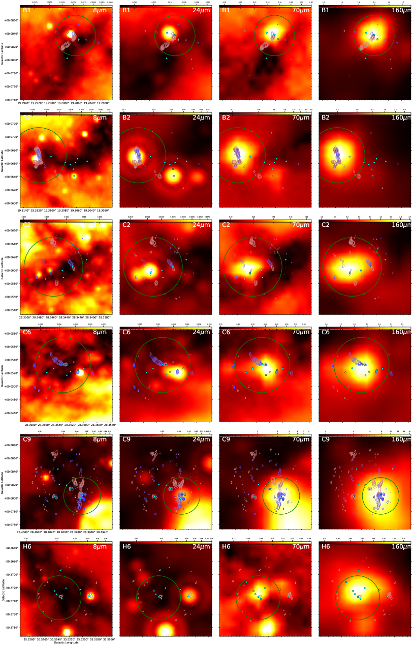
Figure 8: 8 $\mu$m, 24 $\mu$m, 70 $\mu$m and 160 $\mu$m emission of the detected protostars. The color scale is mJy pixel^-1. The blue and red contours denote the blue lobe and the red lobe of SiO outflows, contour levels the same as those in Figure 3. The green circle denotes the aperture size used for building SEDs. The aperture radius is 11″for B1, 15″ for B2, 16″ for C2, 15″ for C6, 10″ for C9 and 12″ for H6. The cyan dots denotes the positions of the 1.3 mm cores.

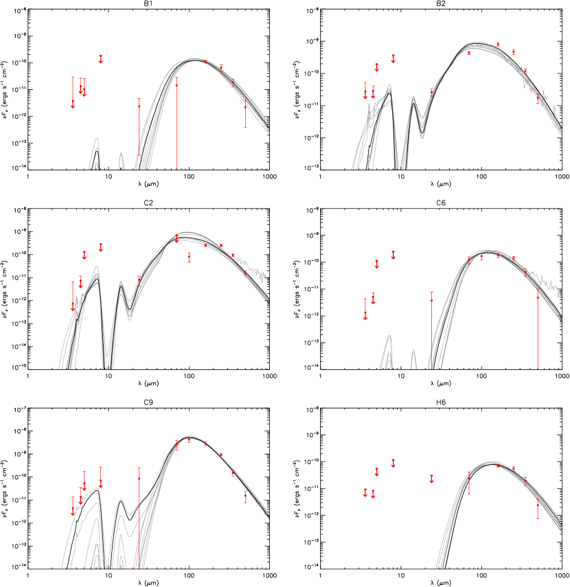
Figure 9: Protostar model fitting to the fixed aperture, background-subtracted SED data using the ZT model grid. For each source, the best fit model is shown with a solid black line and the next nine best models are shown with solid gray lines. Note that the data at $\lesssim 8\>{\rm\mu m}$ are treated as upper limits. If a background subtracted flux density is negative, the flux density without background subtraction is used as upper limits with a negligible error bar (see text). The model parameter results are listed in Table 4.

We investigate the IR emission of the sources that drive the six strongest SiO outflows with Spitzer and Herschel archival data, as shown in Figure 8. This allows us to better understand the nature of the protostars, i.e., by understanding the IR morphologies and comparing to SED models. Note the dynamic range of Figure 8 is set in such a way that faint sources can still show strong contrast. However, the SNR can be very low as in B1, C2, C6 at all wavelengths, B2 at 8 $\mu$m, and H6 at 70 $\mu$m and 160 $\mu$m. The C2, C6, C9 and H6 cores appear dark against the Galactic background at 8 $\mu$m, which indicates they are at an early evolutionary stage. We build spectral energy distributions (SEDs) of the six sources from 3.6 $\rm\mu m$ up to 500 $\rm\mu m$. Given the relatively large beam size of Herschel, we cannot resolve the individual cores revealed with ALMA and the SEDs represent emission from a larger scale region. The circular apertures are determined to include most of the source flux based on their 70 $\mu$m and 160 $\mu$m emission. For B1, C6, C9 and H6, we try to make the apertures centered at the protostar driving the main outflow. The typical aperture size is comparable to the primary beam size of our ALMA 1.3 mm observations.

We fit the fixed aperture, background-subtracted SEDs with the radiative transfer (RT) model developed by Zhang & Tan (2018), which describes the evolution of massive (and intermediate-mass) protostars based on the Turbulent Core model (MT03). The model is described by five physical parameters: the initial core mass ($M_{c}$), the mean mass surface density of the surrounding clump ($\Sigma_{\rm cl}$), the current protostellar mass ($m_{*}$), the foreground extinction ($A_{V}$), and the inclination angle of the outflow axis to the line of sight ($\theta_{\rm view}$). The models describe collapsing cores with bolometric luminosities ranging from 10 $L_{\odot}$ to $10^{7}\ L_{\odot}$ and envelope temperatures from 10 K to 100 K. The evolutionary timescales range from $10^{3}$ yr to $10^{6}$ yr. In the grid of models, $M_{c}$ is sampled at 10, 20, 30, 40, 50, 60, 80, 100, 120, 160, 200, 240, 320, 400, 480 $M_{\odot}$ and $\Sigma_{\rm cl}$ is sampled at 0.10, 0.32, 1, 3.2 $\rm g\ cm^{-2}$, for a total of 60 evolutionary tracks. Then along each track, $m_{*}$ is sampled at 0.5, 1, 2, 4, 8, 12, 16, 24, 32, 48, 64, 96, 128, 160 $M_{\odot}$ (but on each track, the sampling is limited by the final achieved stellar mass, with star formation efficiencies from the core typically being $\sim$ 0.5). There are then, in total, 432 physical models defined by different sets of ($M_{c}$, $\Sigma_{\rm cl}$, $m_{*}$).

The method of deriving SEDs is described in Appendix A. Here we set the data points at wavelengths $\lesssim 8\>{\rm\mu m}$ as upper limits given that PAH emission and transiently heated small grain emission are not well treated in the RT models. In addition, given the high background that can be present in IRDCs at certain wavelengths, sometimes the background subtracted flux density can be negative. In this situation, we use the flux density without background subtraction as upper limits too. These upper limits can be distinguished by a negligible error bar. We note that different aperture sizes can make a significant difference in the flux derived especially for faint sources whose boundaries are not clear. Since we do not know the real distribution of the measurement error, the absolute value of the $\chi^{2}$ is currently dominated by the size of measurement error and does not indicate the goodness of the model well. However, for the same source under the theoretical model we can tell which set of parameters describes the status of the protostar better by comparing their relative values of $\chi^{2}$. For convenience we show the 10 best models. Amongst the best 10 models there can be a significant variation in model parameters, even though the shape of the model SED does not change much, which illustrates degeneracies that exist in trying to constrain protostellar properties from only their MIR to FIR SEDs (see also De Buizer et al. 2017; Rosero et al. 2019a; Liu et al. 2019, 2020). Based on experience, when the best model returns a $\chi^{2}$ smaller than 1 it indicates there are too few valid data points constraining the fitting, so we would consider all the models with $\chi^{2}<2$ among the 10 best models as valid. When the best model returns a $\chi^{2}$ higher than 1, we would consider all the models with $\chi^{2}$ smaller than twice the $\chi^{2}$ of the best model among the 10 best models as valid. For more detailed discussion of the sensitivity of the model to choices in SED construction for faint sources in IRDCs, see Moser et al. (2020). We show the 10 best models for each source in Figure 9. The physical parameters derived are listed in Table 4. Note that these are distinct physical models with differing values of $M_{c}$, $\Sigma_{\rm cl}$ and $m_{*}$, i.e., we do not display simple variations of $\theta_{\rm view}$ or $A_{V}$ for each of these different physical models. The bottom line of each source shows the average results of the valid models. We take the geometric mean for all quantities of the accepted models except $A_{V}$ , $\theta_{\rm view}$, and $\theta_{w,\rm esc}$, where the arithmetic mean is used as in Moser et al. (2020).

By fitting the SEDs with the models, we assume there is one source dominating the infrared luminosity in an aperture. Overall the fitting is reasonable except that the SEDs of B1 and C2 are not clearly characterized due to their bright infrared background. The peaks of the model SEDs seem to locate at a shorter wavelength than the observed SED, which may result in a more evolved stage. In general, considering these six sources and all their 10 best fit models, we find protostellar masses $m_{*}\sim 0.5-8\>M_{\odot}$ accreting at rates of $\sim 10^{-5}-5\times 10^{-4}\>M_{\odot}\>\rm yr^{-1}$ inside cores of initial masses $M_{c}\sim 10-500\>M_{\odot}$ embedded in clumps with mass surface densities $\Sigma_{\rm cl}\sim 0.1-3\>\rm g\>cm^{-2}$ (the full range of $M_{c}$ and $\Sigma_{\rm cl}$ covered by the model grid, though individual sources are more constrained). The disk accretion rates are close to the SiO outflow mass loss rates. The isotropic bolometric luminosity $L_{\rm bol,iso}$ of C9, the most luminous source, is no larger than $10^{4}\>L_{\odot}$. For the other sources $L_{\rm bol,iso}\ \sim 10^{2}-10^{3}\>L_{\odot}$. The half opening angle returned by the best ten models is comparable to the measured half opening angle of the SiO outflow from the ALMA observations for B1. For the other sources generally the half opening angles returned by the models are smaller than what may be inferred from SiO morphologies, if these are to be explained with a single protostellar source. The implications of these SED fitting results are discussed in more detail in §5.2.

Table 4: Parameters of the Ten Best Fitted Models

Source	$\chi^{2}$/N	$M_{\rm c}$	$\Sigma_{\rm cl}$	$R_{core}$	$m_{*}$	$\theta_{\rm view}$	$A_{V}$	$M_{\rm env}$	$\theta_{w,\rm esc}$	$\dot{M}_{\rm disk}$	$L_{\rm bol,iso}$	$L_{\rm bol}$
		($M_{\odot}$)	(g $\rm cm^{-2}$)	(pc) ($\arcsec$)	($M_{\odot}$)	(deg)	(mag)	($M_{\odot}$)	(deg)	($M_{\odot}$/yr)	($L_{\odot}$)	($L_{\odot}$)
B1	1.07	30	0.1	0.13 ( 11 )	0.5	13	657.7	29	10	1.1$\times 10^{-5}$	2.9$\times 10^{2}$	9.0$\times 10^{1}$
$d$ = 2.4 kpc	1.09	20	0.1	0.10 ( 9 )	1.0	22	711.7	17	20	1.3$\times 10^{-5}$	2.7$\times 10^{2}$	1.5$\times 10^{2}$
$R_{ap}$ = 11 ″	1.10	40	0.1	0.15 ( 13 )	0.5	13	717.7	39	8	1.1$\times 10^{-5}$	2.2$\times 10^{2}$	8.8$\times 10^{1}$
= 0.13 pc	1.20	50	0.1	0.16 ( 14 )	0.5	13	755.8	49	7	1.2$\times 10^{-5}$	1.9$\times 10^{2}$	8.7$\times 10^{1}$
	1.31	20	0.1	0.10 ( 9 )	4.0	51	999.0	10	43	2.1$\times 10^{-5}$	2.9$\times 10^{2}$	6.8$\times 10^{2}$
	1.32	10	0.3	0.04 ( 4 )	1.0	29	922.9	8	28	2.5$\times 10^{-5}$	5.3$\times 10^{2}$	2.6$\times 10^{2}$
	1.34	60	0.1	0.18 ( 15 )	0.5	13	798.8	59	6	1.3$\times 10^{-5}$	1.7$\times 10^{2}$	8.7$\times 10^{1}$
	1.35	20	0.1	0.10 ( 9 )	0.5	22	468.5	19	13	9.6$\times 10^{-6}$	8.6$\times 10^{1}$	9.0$\times 10^{1}$
	1.37	20	0.1	0.10 ( 9 )	2.0	13	617.6	15	30	1.7$\times 10^{-5}$	8.3$\times 10^{2}$	1.9$\times 10^{2}$
	1.40	30	0.1	0.13 ( 11 )	2.0	89	1000.0	25	23	2.0$\times 10^{-5}$	1.4$\times 10^{2}$	2.4$\times 10^{2}$
Averages	1.25	27	0.1	0.11 ( 10 )	0.9	28	765.0	22	19	1.5$\times 10^{-5}$	2.5$\times 10^{2}$	1.5$\times 10^{2}$
B2	6.26	200	0.1	0.33 ( 28 )	2.0	13	233.2	194	7	3.5$\times 10^{-5}$	7.3$\times 10^{2}$	3.5$\times 10^{2}$
$d$ = 2.4 kpc	6.64	240	0.1	0.36 ( 31 )	1.0	13	126.1	240	4	2.6$\times 10^{-5}$	3.2$\times 10^{2}$	2.4$\times 10^{2}$
$R_{ap}$ = 15 ″	6.65	100	0.1	0.23 ( 20 )	2.0	13	279.3	97	11	2.9$\times 10^{-5}$	1.2$\times 10^{3}$	3.8$\times 10^{2}$
= 0.17 pc	6.72	120	0.1	0.25 ( 22 )	2.0	13	287.3	117	9	3.0$\times 10^{-5}$	1.2$\times 10^{3}$	4.3$\times 10^{2}$
	6.80	320	0.1	0.42 ( 36 )	1.0	13	81.1	315	3	2.8$\times 10^{-5}$	2.5$\times 10^{2}$	2.0$\times 10^{2}$
	7.04	160	0.1	0.29 ( 25 )	2.0	13	273.3	156	8	3.3$\times 10^{-5}$	1.0$\times 10^{3}$	4.3$\times 10^{2}$
	7.68	80	0.1	0.21 ( 18 )	2.0	13	277.3	75	12	2.7$\times 10^{-5}$	1.3$\times 10^{3}$	3.5$\times 10^{2}$
	7.92	320	0.3	0.23 ( 20 )	96.0	89	378.4	7	85	6.6$\times 10^{-5}$	2.2$\times 10^{3}$	1.2$\times 10^{6}$
	7.99	200	0.1	0.33 ( 28 )	1.0	13	101.1	197	4	2.5$\times 10^{-5}$	2.7$\times 10^{2}$	1.8$\times 10^{2}$
	7.99	160	0.1	0.29 ( 25 )	1.0	13	128.1	156	5	2.3$\times 10^{-5}$	3.3$\times 10^{2}$	2.0$\times 10^{2}$
Averages	7.14	173	0.1	0.29 ( 25 )	2.2	20	216.5	114	15	3.1$\times 10^{-5}$	6.9$\times 10^{2}$	6.7$\times 10^{2}$
C2	5.69	480	0.1	0.51 ( 21 )	4.0	13	253.3	474	6	6.1$\times 10^{-5}$	1.8$\times 10^{3}$	1.0$\times 10^{3}$
$d$ = 5.0 kpc	6.13	400	0.1	0.47 ( 19 )	4.0	13	266.3	390	7	5.8$\times 10^{-5}$	2.0$\times 10^{3}$	1.0$\times 10^{3}$
$R_{ap}$ = 16 ″	6.50	320	0.3	0.23 ( 10 )	96.0	62	520.5	7	85	6.6$\times 10^{-5}$	1.3$\times 10^{6}$	1.2$\times 10^{6}$
= 0.39 pc	8.54	480	0.1	0.51 ( 21 )	2.0	13	133.1	477	4	4.3$\times 10^{-5}$	7.4$\times 10^{2}$	5.7$\times 10^{2}$
	8.66	240	0.1	0.36 ( 15 )	4.0	13	289.3	229	9	5.1$\times 10^{-5}$	2.7$\times 10^{3}$	1.0$\times 10^{3}$
	9.19	320	0.3	0.23 ( 10 )	2.0	13	169.2	314	4	9.2$\times 10^{-5}$	1.4$\times 10^{3}$	1.1$\times 10^{3}$
	9.35	200	0.3	0.19 ( 8 )	4.0	13	328.3	193	9	1.1$\times 10^{-4}$	4.3$\times 10^{3}$	1.4$\times 10^{3}$
	9.53	200	0.3	0.19 ( 8 )	2.0	13	232.2	196	6	8.2$\times 10^{-5}$	2.0$\times 10^{3}$	1.2$\times 10^{3}$
	9.53	240	0.3	0.20 ( 8 )	2.0	13	226.2	235	5	8.6$\times 10^{-5}$	1.8$\times 10^{3}$	1.2$\times 10^{3}$
	9.55	160	0.3	0.17 ( 7 )	4.0	13	314.3	153	11	1.1$\times 10^{-4}$	4.3$\times 10^{3}$	1.2$\times 10^{3}$
Averages	8.12	285	0.2	0.28 ( 11 )	4.2	18	273.3	188	15	7.3$\times 10^{-5}$	3.9$\times 10^{3}$	2.1$\times 10^{3}$
C6	0.88	480	0.1	0.51 ( 21 )	2.0	13	642.6	477	4	4.3$\times 10^{-5}$	7.4$\times 10^{2}$	5.7$\times 10^{2}$
$d$ = 5.0 kpc	0.96	240	0.1	0.36 ( 15 )	4.0	13	935.9	229	9	5.1$\times 10^{-5}$	2.7$\times 10^{3}$	1.0$\times 10^{3}$
$R_{ap}$ = 15 ″	0.97	400	0.1	0.47 ( 19 )	2.0	13	591.6	391	4	4.1$\times 10^{-5}$	7.7$\times 10^{2}$	5.5$\times 10^{2}$
= 0.36 pc	1.10	400	0.1	0.47 ( 19 )	4.0	89	961.0	390	7	5.8$\times 10^{-5}$	9.4$\times 10^{2}$	1.0$\times 10^{3}$
	1.13	320	0.1	0.42 ( 17 )	4.0	13	536.5	308	7	5.5$\times 10^{-5}$	1.2$\times 10^{3}$	5.4$\times 10^{2}$
	1.20	480	0.1	0.51 ( 21 )	4.0	89	974.0	474	6	6.1$\times 10^{-5}$	9.2$\times 10^{2}$	1.0$\times 10^{3}$
	1.25	160	0.1	0.29 ( 12 )	4.0	13	757.8	151	12	4.5$\times 10^{-5}$	3.1$\times 10^{3}$	9.1$\times 10^{2}$
	1.27	200	0.3	0.19 ( 8 )	1.0	13	725.7	196	4	5.8$\times 10^{-5}$	6.5$\times 10^{2}$	5.2$\times 10^{2}$
	1.34	200	0.1	0.33 ( 14 )	4.0	13	605.6	194	10	4.8$\times 10^{-5}$	1.9$\times 10^{3}$	6.7$\times 10^{2}$
	1.42	320	0.3	0.23 ( 10 )	96.0	68	1000.0	7	85	6.6$\times 10^{-5}$	1.1$\times 10^{6}$	1.2$\times 10^{6}$
Averages	1.14	299	0.1	0.36 ( 15 )	4.2	33	773.1	198	15	5.2$\times 10^{-5}$	2.4$\times 10^{3}$	1.5$\times 10^{3}$
C9	1.14	160	3.2	0.05 ( 2 )	2.0	13	214.2	158	5	4.4$\times 10^{-4}$	8.5$\times 10^{3}$	5.2$\times 10^{3}$
$d$ = 5.0 kpc	1.20	120	3.2	0.05 ( 2 )	4.0	13	646.6	113	11	5.7$\times 10^{-4}$	4.0$\times 10^{4}$	1.1$\times 10^{4}$
$R_{ap}$ = 10 ″	1.25	120	3.2	0.05 ( 2 )	8.0	13	951.0	106	15	7.9$\times 10^{-4}$	1.2$\times 10^{5}$	1.9$\times 10^{4}$
= 0.24 pc	1.33	240	1.0	0.11 ( 5 )	8.0	13	854.9	223	11	4.0$\times 10^{-4}$	4.4$\times 10^{4}$	1.4$\times 10^{4}$
	1.35	400	1.0	0.15 ( 6 )	4.0	13	158.2	394	5	3.3$\times 10^{-4}$	6.7$\times 10^{3}$	4.7$\times 10^{3}$
	1.42	240	0.3	0.20 ( 8 )	12.0	86	1000.0	216	15	2.0$\times 10^{-4}$	3.1$\times 10^{4}$	4.1$\times 10^{4}$
	1.43	480	1.0	0.16 ( 7 )	4.0	13	233.2	478	5	3.4$\times 10^{-4}$	6.6$\times 10^{3}$	5.0$\times 10^{3}$
	1.43	400	0.1	0.47 ( 19 )	16.0	89	767.8	364	17	1.1$\times 10^{-4}$	2.7$\times 10^{4}$	3.8$\times 10^{4}$
	1.43	320	0.1	0.42 ( 17 )	24.0	89	927.9	256	27	1.2$\times 10^{-4}$	4.4$\times 10^{4}$	8.4$\times 10^{4}$
	1.44	100	3.2	0.04 ( 2 )	12.0	77	1000.0	77	20	9.4$\times 10^{-4}$	2.5$\times 10^{4}$	5.2$\times 10^{4}$
Averages	1.34	225	0.9	0.12 ( 5 )	7.3	42	675.4	204	13	3.4$\times 10^{-4}$	2.4$\times 10^{4}$	1.7$\times 10^{4}$
H6	0.56	80	0.1	0.21 ( 15 )	0.5	89	1000.0	79	5	1.4$\times 10^{-5}$	8.6$\times 10^{1}$	9.2$\times 10^{1}$
$d$ = 2.9 kpc	0.57	60	0.1	0.18 ( 13 )	0.5	34	888.9	59	6	1.3$\times 10^{-5}$	8.6$\times 10^{1}$	8.7$\times 10^{1}$
$R_{ap}$ = 12 ″	0.61	50	0.1	0.16 ( 12 )	0.5	22	841.8	49	7	1.2$\times 10^{-5}$	8.7$\times 10^{1}$	8.7$\times 10^{1}$
= 0.17 pc	0.65	100	0.1	0.23 ( 17 )	0.5	89	1000.0	99	4	1.5$\times 10^{-5}$	8.7$\times 10^{1}$	9.1$\times 10^{1}$
	0.68	30	0.1	0.13 ( 9 )	1.0	86	1000.0	27	15	1.5$\times 10^{-5}$	1.3$\times 10^{2}$	1.7$\times 10^{2}$
	0.71	120	0.1	0.25 ( 18 )	0.5	86	1000.0	118	4	1.5$\times 10^{-5}$	8.4$\times 10^{1}$	8.8$\times 10^{1}$
	0.72	40	0.1	0.15 ( 10 )	0.5	13	806.8	39	8	1.1$\times 10^{-5}$	2.2$\times 10^{2}$	8.8$\times 10^{1}$
	0.73	30	0.1	0.13 ( 9 )	2.0	89	1000.0	25	23	2.0$\times 10^{-5}$	1.4$\times 10^{2}$	2.4$\times 10^{2}$
	0.98	30	0.1	0.13 ( 9 )	0.5	22	703.7	29	10	1.1$\times 10^{-5}$	8.8$\times 10^{1}$	9.0$\times 10^{1}$
	1.01	40	0.1	0.15 ( 10 )	1.0	89	1000.0	38	12	1.6$\times 10^{-5}$	1.3$\times 10^{2}$	1.7$\times 10^{2}$
Averages	0.71	51	0.1	0.17 ( 12 )	0.7	62	924.1	49	10	1.4$\times 10^{-5}$	1.1$\times 10^{2}$	1.1$\times 10^{2}$

Note. — For each source, the values in the first row are derived using our fiducial method that uses the full velocity range for the integration of SiO emission and with $t_{\rm dyn}$ evaluated with an average outflow velocity. Values of $t_{\rm dyn}$ outside and inside parentheses use mass and momentum weighted velocities, respectively. The results in the second row for each source are derived in the same way as the first row, except that $t_{\rm dyn}$ is evaluated by using the maximum observed outflow velocity. The values in the third row are as as the first row, except that SiO emission within $\pm$ 3 km s^-1 of the systemic velocity is excluded. The values in the fourth row are derived in the same way as the third row, except that $t_{\rm dyn}$ is evaluated by using the maximum observed outflow velocity.

3.3 Weak SiO Sources

As shown in Figure 1, while in some clumps there is a good indication of the location of the driving source of the SiO emission, e.g., A1, D9, and E2, where a continuum source is located in between two patches of SiO emission, in other clumps the situation is more uncertain. The shape of the SiO emission also varies – in A1, A2 and C4 the main SiO emission is relatively elongated, in D8 and H5 it appears more rounded, and in other cases SiO is hardly resolved. We investigate the kinematics of the SiO(5-4) emission via the channel maps of each source and try to locate the driving source assuming the SiO emission comes from an outflow.

For the sources that show relatively strong SiO emission (see Figure 2), like A1, A2, C4, D8, H5, from their channel maps the velocity range of the SiO emission above 3$\sigma$ noise level exceeds 6 km $\rm s^{-1}$. Duarte-Cabral et al. (2014) suggested that narrow line SiO emission ($\sigma_{v}<$ 1.5 km s^-1, i.e., line width $<$ 3.5 km s^-1) appears unrelated to outflows, but rather traces large scale collapse of material onto massive dense cores (see also Cossentino et al. 2018, 2020). Thus, in this context, in these five sources it is more likely that SiO traces shocks from outflows. In A1 there are two components revealed in Figure 1, while the northern component appears to be red-shifted and the southern component appears to be blue-shifted (see also §4). In A2 the large extended emission in the center of the field (see Figure 1) shows a hint of bipolar structure with the blue-shifted emission to the east of the field center and the red-shifted emission to the west. In C4, D8 and H5, no clear bipolar structure is seen.

In other sources the signal to noise ratio of SiO emission is low and most of the time the emission above the 3$\sigma$ noise level in the channel maps appears as an unresolved peak and the velocity range does not exceed 4 km $\rm s^{-1}$. In D9 the northern component appears blue-shifted and the southern component red-shifted. In E2 there is a hint that the eastern component is blue-shifted relative to the source velocity and the western component red-shifted, though the emission is not stronger than the 2$\sigma$ noise level. There is hardly any bipolar outflow structure revealed in the other sources. Thus for these sources we are not sure whether the SiO emission comes from protostellar outflows.

Overall, in A1, A2, D9, and E2 there is a hint of bipolar structures revealed in the channel maps. For A1, D9, and E2, the continuum source located in the middle of the two patches of SiO emission is likely responsible for driving the elongated SiO outflows. In sources like A2, the driving source of SiO is ambiguous. The emission of the dense gas tracers at the continuum peaks and the SiO peaks are all very weak. D8 is another example of an ambiguous SiO driving source. The velocity range of the central SiO emission is as wide as 30 km $\rm s^{-1}$, thus the SiO is not likely from large-scale cloud collision (Duarte-Cabral et al. 2014). The integrated intensity of the central SiO is even higher than H6. In D1, D3 and D8 the 1.3 mm continuum cores are not associated with any detectable dense gas tracers.

The SED fitting results for these sources are presented in Appendix A. Most of the SEDs are not well defined, likely because most sources are very young and even appear dark against the background at 70 $\mu$m. The stellar masses of the valid models range from 0.5 $M_{\odot}$ to 4 $M_{\odot}$. The isotropic luminosities ranges from $10^{2}\>L_{\odot}$ to $10^{3}\>L_{\odot}$.

4 6 cm Radio Emission

We searched for 6 cm radio emission in the ALMA field of view ($\sim$ 27″in diameter) of each clump. Out of the 15 clumps that exhibit strong SiO outflows observed with VLA, we only detected radio emission above the 3 $\sigma$ noise level in four sources A1, C2, C4, C9. The peak positions and flux measurements of the 6 cm radio continuum are reported in Table 5. The radio continuum emission is shown in Figure 10. The emission in A1, C2 and C4 is hardly resolved, while the emission in C9 is resolved into two peaks. The negative artifacts are not significant with no stronger than -2 $\sigma$ level in C2 and C9 and no stronger than -3 $\sigma$ level in A1 and C4. We note that the low detection rate of 6 cm radio emission may be partly due to limited sensitivities. The sensitivities of the 6 cm images vary by a factor of almost 3, and the detections in A1, C2, and C4 come from images that achieves a higher sensitivity than others in the same cloud, while in the B and D cloud, where no 6 cm emission is detected, the sensitivity is much worse.

In Sanna et al. (2018), the detection rate of 22 GHz continuum emission towards 25 H₂O maser sites is 100% and they suggested H₂O masers are preferred signposts of bright radio thermal jets ($\gg$ 1mJy). Here we see coincidence of 6 GHz radio continuum emission and H₂O masers at C2c4 and C4c1.

We attempt to derive the in-band spectra index, $\alpha$, of the two sources in C9, i.e., assuming $F_{\nu}\propto\nu^{\alpha}$, by dividing the continuum data into two centered at 5.03 GHz and 6.98 GHz respectively. In A1, C2 and C4 the sources detected in the combined continuum data do not have enough signal to noise for such an estimate. We derive an $\alpha$ of -0.52 for C9r1 and -2.36 for C9r2. However, as discussed in Rosero et al. (2016), the in-band spectral index derived from only two data points can be highly uncertain and more measurements at other wavelengths are required for confirmation of these results.

There are offsets between the radio continuum peak and the 1.3mm continuum peak in all the sources, typically about 500 mas, i.e., about 1 VLA synthesized beam width and corresponding to $\sim$ 2500 AU. Such offsets likely indicate that the radio emission comes from jet lobes and/or that the offset is due to a gradient in the optical depth. Another possibility is that the offset is due to astrometric uncertainties in the VLA data, but this would require an uncertainty several times larger than we have estimated ($\lesssim$ 170 mas). This error takes into account the accuracy of the phase calibrator and VLA antenna positions, the transfer of solutions from the phase calibrator to the target, and the statistical error in measuring the source’s peak position. The unresolved emission in A1, C2 and C4 basically follows the direction and shape of the VLA beam and it is hard to compare with the direction of the outflows. The extension of the emission in C9 is not along the direction of the large scale north-south outflow. However, it could be related to the small scale outflows in the region.

Table 5: Parameters of 6 cm Radio Continuum

Source	R.A.	Decl.	$I_{\rm peak}$	$S_{\rm 6GHz}$
	(J2000)	(J2000)	($\mu$Jy beam-1)	($\mu$Jy)
A1	18:26:15.442	-12:41:37.505	14.44	24.14
C2r1	18:42:50.228	-4:03:21.022	31.37	24.80
C2r2	18:42:50.762	-4:03:11.534	21.79	68.65
C4	18:42:48.724	-4:02:21.433	13.16	5.85
C9r1	18:42:51.979	-3:59:54.534	40.05	47.70
C9r2	18:42:51.979	-3:59:53.734	35.87	46.97

Figure 10: 6 cm radio emission and SiO outflow emission over 1.3 mm continuum. White contours are the 6 cm radio continuum. Blue and red contours are the blue- and red-shifted SiO integrated intensity. Grayscale is the 1.3mm continuum. Plus signs denote the 1.3mm continuum peaks. The beam size of the ALMA 1.3 mm continuum observations is shown in the lower left corner. The beam size of the VLA 6 cm continuum observations is shown in the lower right corner. The images have a field of view of 16″$\times$ 16″.

5 Discussion

5.1 SiO Detection Rate

We have detected SiO(5-4) emission in 20 out of 32 IRDC clumps, a detection rate of 62%. Our sample has a distance range of 2.4-5.7 kpc. The cloud with the lowest detection rate, Cloud F, is located at a moderate distance of 3.7 kpc. The cloud with the highest detection rate, cloud D, happens to be located at the largest distance. Thus the detection rate does not appear to have a strong dependence on distance. López-Sepulcre et al. (2011) derived an SiO detection rate of 88% towards 20 high-mass ($M_{\rm clump}\gtrsim\ 100\>M_{\odot}$) IR-dark clumps (not detected at 8 $\mu$m with the Midcourse Space eXperient (MSX)) with SiO(2-1) and SiO(3-2). Csengeri et al. (2016) derived an SiO detection rate of 61% towards 217 IR-quiet clumps (a threshold of 289 Jy at 22 $\mu$m at 1 kpc) with SiO(2-1). In particular, the SiO detection rate is 94% for a subsample of clumps with $M_{\rm clump}>650\>M_{\odot}$ and 1 kpc $<d<$ 7 kpc. With a more evolved sample, Harju et al. (1998) derived an SiO detection rate of 38% for protostars above $10^{3}\>L_{\odot}$ with SiO(2-1) and SiO(3-2). Gibb et al. (2007) detected SiO emission in five out of 12 (42%) massive protostars with SiO(5-4). Li et al. (2019a) detected SiO(5-4) emission in 25 out of 44 IRDCs with a detection rate of 57%, and 32 out of 86 protostars in massive clumps (a subsample defined to be at the intermediate evolutionary stage between IRDCs and HII regions) with a detection rate of 37%.

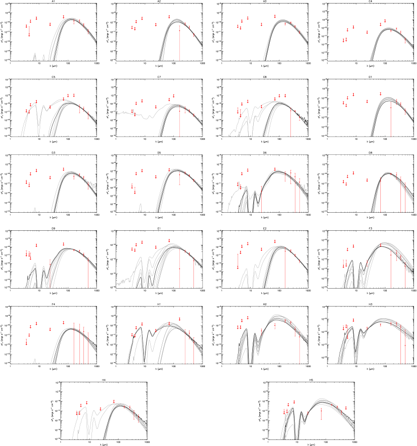
Figure 18: The same with Figure 9 but for weak SiO sources. The model parameter results are listed in Table 6.

Our result is similar to that of the full sample of Csengeri et al. (2016) and the IRDC sample of Li et al. (2019a). The clumps in our sample are not as massive as those of López-Sepulcre et al. (2011). In Liu et al. (2018), seven of the 1.3 mm continuum cores (C2c2, C2c3, C2c4, C9c5, C9c7, C9c8, D9c2) are high-mass protostellar candidates, i.e., with masses $>25\>M_{\odot}$, assuming a core-to-star efficiency of about 30%. Twelve others (A1c2, A3c3, C2c1, C4c1, C4c2, C6c1, C6c5, C6c6, C9c6, D5c6, D6c1, D6c4) are intermediate-mass protostellar candidates, i.e., with masses in the range 9 to 24 $M_{\odot}$. The non-detection of SiO tends to be in clumps with weak or non-detected 1.3 mm continuum emission ($M_{\rm core}<5\>M_{\odot}$, Liu et al. 2018), and dark against background up to 100 $\mu$m (except for source H2, see Figure 18 in Appendix A). This indicates in IRDCs, representative of the earliest evolutionary phases, shocked gas is more common in the higher mass regime. The non-detections may reflect the more diffuse clumps without star formation as suggested in Csengeri et al. (2016). However, as discussed in §3.1, there is possible large scale SiO emission in those regions, which is resolved out with our observations. On the other hand, we do see SiO emission in clumps with only low-mass 1.3 mm cores detected and low luminosity. Overall, compared with more evolved IR bright protostars in Harju et al. (1998) and Gibb et al. (2007), the detection rate of SiO in our sample, most of which have a luminosity $<\>10^{3}\>L_{\odot}$ and still appear dark against background at 70 $\mu$m, and other early stage IR-quiet protostars (López-Sepulcre et al. 2011, Csengeri et al. 2016, Li et al. 2019a), is higher.

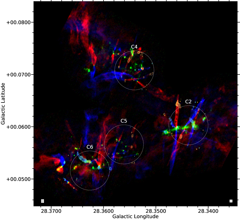
Figure 11: Map of molecular outflows in part of Cloud C. The RGB colorscale mosaic is the same with Figure 1 in Kong et al. (2019), where green represents 1.3 mm continuum emission observed with 0.5″resolution, blue represents blue-shifted CO(2-1) emission, integrated from 11.7 to 75.4 km s^-1, and red represents red-shifted CO(2-1) emission, integrated from 83.2 to 146.9 km s^-1. The cyan and orange contours represent blue- and red-shifted SiO outflows observed in this paper. Contour levels start at 5$\sigma$ in steps of 4$\sigma$ noise level of the integrated intensity (see Section 3.2.1. The dashed circles denote the primary beams of the observations presented in this paper. The beam size of the SiO outflows is shown in the lower left corner. The beam size of Kong et al. (2019) observations is shown in the lower right corner.

For sources in the C2, C4, C5 and C6 regions of Cloud C we are able to make a direct comparison of the SiO emission with previously reported CO(2-1) outflow data from Kong et al. (2019). As shown in Figure 11, we see that CO outflow emission is generally more common and more widespread than that from SiO, which is more “sparse”, i.e., localized to parts of a given CO outflow. The CO outflows are highly collimated. Because of its sparse appearance, SiO typically appears to have a less collimated morphology than the CO outflows. One reason why we do not see clear collimated outflows with SiO(5-4) as with CO(2-1) is the high critical density of the SiO(5-4) transition ($\sim 2.5\times 10^{6}\rm\>cm^{-3}$), implying that only high density shocked regions can be detected with this transition. Such high-density gas may also be confined in regions narrower than the synthesized beam, resulting in a diluted signal that is more difficult to detect than the more extended CO(2-1). Comparing to the results of Kong et al. (2019) and Liu et al. (2018), we find 3 overlapping identified 1.3 mm continuum sources (those with $<$ 1″difference in core coordinates) in C2 (C2c2, C2c3, C2c4), 4 in C4 (C4c1, C4c2, C4c6, C4c8), 4 in C5 (C5c2, C5c4, C5c5, C5c6), and 4 in C6 (C6c1, C6c2, C6c5, C6c6). In C2, the main SiO outflow driven by C2c2 does not align with the main CO outflow, but there seems to be a secondary weak CO in that direction especially revealed in the blue-shifted side. Other than that we see several patches of SiO emission overlapping with CO outflows with the same direction relative to the plane of sky. In C6 the main blue-shifted SiO outflow driven by C6c1 aligns very well with the blue-shifted CO outflow. The red-shifted SiO outflow in the opposite direction is relatively weak, and we do not see strong red-shifted CO outflow coming from the west of C6c1 either. The SiO emission associated with C6c5 aligns well with the bipolar CO outflow. Outside of the primary beam of C6 we also see several overlaps of the SiO emission with the CO outflows. In C4 and C5 the SiO emission is relatively weak, but, still, where we detect SiO emission, most of the time there are also CO outflows with the same direction relative to the plane of sky. Our results partly agree with the results in Li et al. (2019b), who detect SiO(5-4) emission only in 6 out of 17 IRDC protostellar sources with detected CO(2-1) outflows. They find that the SiO emission is much fainter and has a narrower velocity range ($10-15\rm km\ s^{-1}$) than that of the CO emission. While the strong SiO emission in their sample still overlaps with CO outflows, the weak SiO emission features are generally not associated with CO (see their Figure 2).

5.2 Characteristics of the Protostellar Sources

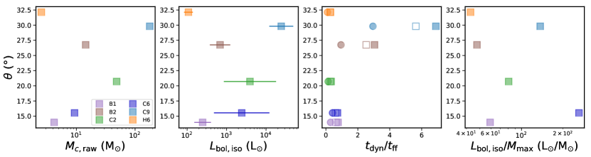
Figure 12: Outflow half opening angle $\theta$ versus the mm core mass $M_{c,\rm raw}$, isotropic bolometric luminosity $L_{\rm bol,iso}$, the ratio of outflow dynamical time scale over free-fall time scale $t_{\rm dyn}/t_{\rm ff}$, and luminosity to mass ratio $L_{\rm bol,iso}/M_{\rm max}$. The filled squares represent outflow parameters derived with the fiducial method, i.e., using the full velocity range and $t_{\rm dyn}$ derived with an average outflow velocity. The filled circles represent outflow parameters derived with the full velocity range and $t_{\rm dyn}$ derived with the maximum outflow velocity. The empty squares represent outflow parameters derived excluding the emission within $\pm$ 3 km s^-1 to the systemic velocity, which we consider coming from ambient gas, and $t_{\rm dyn}$ derived with an average outflow velocity. The error bar represents 95% geometric confidence interval of $L_{\rm bol,iso}$ among the valid models.

We investigate the potential correlations between outflow collimation and core mass, luminosity, time scale, luminosity-to-mass ratio, etc., for the strong SiO sources as shown in Figure 12. The half opening angles are directly measured from the SiO outflows associated with individual protostellar sources observed by ALMA. $M_{c,\rm raw}$ and $M_{\rm max}$ are derived from the 1.3 mm continuum emission. Note the outflow half opening angle and the dynamical time adopt the values of the representative flow of each source, i.e., red flow for B1, B2, H6 and blue flow for C2, C6 and C9. The free-fall time is derived from $t_{\rm ff}=\sqrt{\frac{3\pi}{32G\rho}}$. $\rho$ is derived from the 1.3mm dust continuum core mass from Liu et al. (2018). Here for $L_{\rm bol,iso}/M_{\rm max}$ in each source, we use the mass of the one main core driving the outflows (B1c2, B2c9, C2c2, C6c1, C9c5, H6c8) from Liu et al. (2018), which happens to be the most massive core in each field, and assumes the bolometric luminosity derived from the SED fitting mainly comes from this core. The collimation of the outflow lobes that are not very extended, like H6, may be influenced if they were to be corrected for inclination. Overall, if assuming the same inclination for every source, i.e., with no relative effects of inclination, we do not see apparent correlations between outflow opening angles and evolutionary stage. Note that if we exclude B2 and H6, which have a poorly defined outflow opening angle, we do see that the outflow opening angle increases as core mass and luminosity increase in the other four sources.

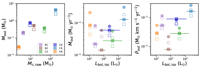
Figure 13: From left to right: outflow mass $M_{\rm out}$ versus the mm core mass $M_{c,\rm raw}$, outflow mass rate $\dot{M}_{\rm out}$ versus isotropic bolometric luminosity $L_{\rm bol,iso}$, outflow momentum rate $\dot{P}_{\rm out}$ versus isotropic bolometric luminosity $L_{\rm bol,iso}$. The symbols are the same with Figure 12, with the additional empty circles representing outflow parameters derived excluding the emission within $\pm$ 3 km s^-1 to the systemic velocity, which we consider coming from ambient gas, and $t_{\rm dyn}$ derived with the maximum outflow velocity.

We also investigate the mass entrainment of the strong SiO outflows as shown in Figure 13. The outflow mass seems to increase with the core mass, which is consistent with the results of Beuther et al. (2002). Previous outflow studies have also found correlation between the bolometric luminosity and the mechanical force and momentum, which holds over six orders of magnitude of $L_{\rm bol}$ (e.g., Figure 4 in Beuther et al. 2002, Figure 7 in Maud et al. 2015), and is interpreted as evidence for a single outflow mechanism that scales with the stellar luminosity, and the outflows motion being momentum driven. From the six sources presented here, the potential correlation of the mechanical force and mass entrainment rate with luminosity has significant scatter.

Since we can only resolve the protostellar cores down to a typical scale of 5000 AU, we are unable to further distinguish the outflow launching mechanism (e.g., the X-wind model (Shu et al. 2000) and the disk-wind model (Königl & Pudritz 2000)).

H₂O maser emission traces shocked gas propagating in dense regions ($n_{H_{2}}>10^{6}\rm\>cm^{-3}$) at velocities between 10 and 200 km s^-1 (e.g., Hollenbach et al. 2013) and is considered to be a signpost of protostellar outflows within a few 1000 AU of the driving source. Surveys have found H₂O masers associated with young stellar objects with luminosities of $1-10^{5}\>L_{\odot}$ (Wouterloot & Walmsley 1986; Churchwell et al. 1990; Palla et al. 1993; Claussen et al. 1996). Wang et al. (2006) observed $\rm H_{2}O$ maser emission toward a sample of 140 compact, cold IRDC cores with the VLA. All the 32 regions except for C9 are covered by their observation. Only at B2c8 (0.66 $M_{\odot}$), C2c4 (33 $M_{\odot}$), C4c1 (17 $M_{\odot}$), D5c1 (3.6 $M_{\odot}$) are water masers detected with emission higher than the detection limit of 1 Jy (see Figure 3). They have a relatively low detection rate of 12% and suggest that most of the IRDC cores have not yet formed high-mass protostars or are forming only low- or intermediate-mass protostars. While more of our sources are at an early evolutionary stage, as indicated by the SED fitting, we do have some massive cores in B2, C2 and D9 (C9 has the most massive cores and appears most evolved but it is not covered in the Wang et al. (2006) observations). We think sensitivity is likely to be a major limiting factor here. Our VLA observations are sensitive to CH₃OH masers, which trace high-mass star formation. The CH₃OH maser results will be presented in a later paper (Rosero et al. in prep.). From an initial inspection, it appears that there is only detection in the B2 and C9 clump (associated with the C9r1 core).

Compared with the SED fitting results of more evolved massive YSOs (De Buizer et al. 2017; Liu et al. 2019, 2020), the accretion rates $\dot{M}_{\rm disk}$ derived in our IRDC sample are about one order of magnitude lower even for the high-/intermediate-mass sources, though the photometry scale may be smaller by a factor of 2. Further comparison of protostellar properties of the sources studied here and those of the SOMA survey sample has been presented by Liu et al. (2020). The low luminosity, low accretion rates and low current stellar mass returned by SED fitting suggest the sources in our sample are at an early stage.

5.3 Strength of SiO Emission

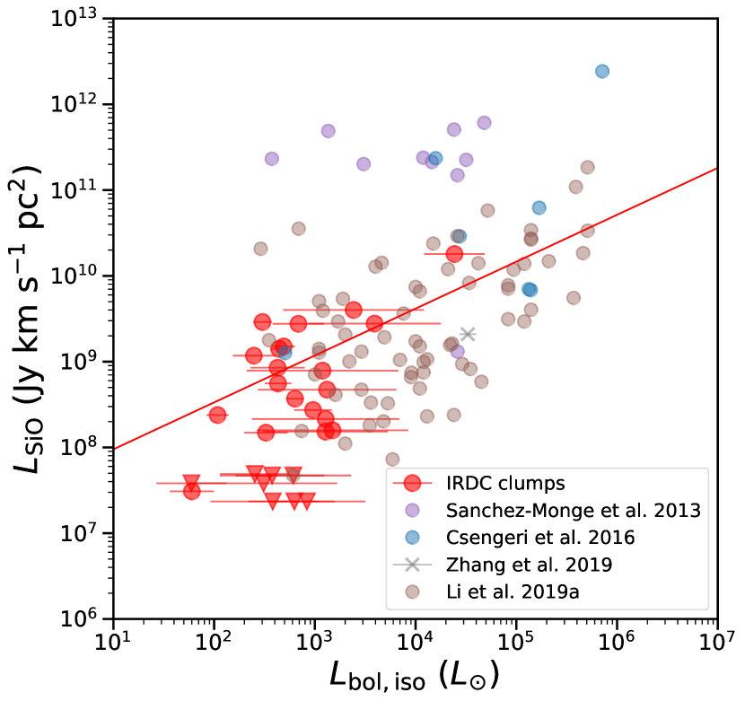
Figure 14: SiO(5-4) line luminosity $L_{\rm SiO}$ as a function of protostar bolometric luminosity $L_{\rm bol,iso}$. The red dots denote our SiO(5-4) data, while the red triangles indicate upper limits for SiO line luminosity. The error bar represents 95% geometric confidence interval of $L_{\rm bol,iso}$ among the valid models. The purple dots denote SiO(5-4) data from Sánchez-Monge et al. (2013b). The blue dots denote SiO(5-4) data from Csengeri et al. (2016). The brown dots denote SiO(5-4) data from Li et al. (2019). The gray cross denotes SiO(5-4) data from Zhang et al. (2019). The red line shows a linear fit $f(x)=0.55x+7.43$.

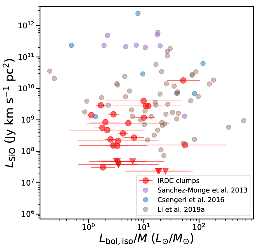
Figure 15: SiO(5-4) line luminosity $L_{\rm SiO}$ as a function of the bolometric luminosity-mass ratio $L_{\rm bol,iso}/M$. The markers are the same as in Figure 14. The error bar represents 95% geometric confidence interval of $L_{\rm bol,iso}$ among the valid models.

We measured the bolometric luminosity of the sources defined by their MIR emission (geometric mean $L_{\rm bol,iso}$ of the valid models in the ten best models of each source) and the SiO line luminosity inside the aperture to explore how SiO acts as an outflow tracer across the luminosity regime. The flux inside the contours denoting trunk structures in Figure 1 is used to calculate the SiO line luminosity. For the 6 sources for which we have accurate velocity range estimates, we remade their integrated intensity maps using the updated velocity range and derived new trunk structures with astrodendro. For the other sources, we adopted a universal velocity range of $\pm$15 km s^-1 relative to the systemic velocity for all the sources, given that the SNRs for more than half of the 32 sources are too low to determine a distinct velocity range. For most sources this velocity range represents the SiO emission well. We sum up flux from all the trunks inside the ALMA field of view for each source. Note that in B2 and C9, we only include part of the SiO which is inside the apertures shown in Figure 8. For all the other sources almost all the detected SiO emission falls inside the aperture used for photometry.

The results are shown in Figure 14. Where there is SiO, we can always find 1.3 mm continuum emission and some infrared emission nearby, but not vice versa. Those clumps with no detectable SiO emission are denoted with 3 $\sigma$ SiO detection thresholds in Figure 14. In C3 and D2 there is neither SiO or 1.3 mm continuum cores detected, so we think there are no protostars in these two clumps and do not measure the luminosities there. We also include measurement of SiO(5-4) from the literature. We notice there may be biases to combine the data due to differences in instrument and method. Nevertheless, we see a slight increasing trend of SiO line luminosity with the bolometric luminosity. We obtain a linear fit of $f(x)=(0.55\pm 0.09)x+(7.43\pm 0.37)$ and the Pearson correlation coefficient is $\sim$ 0.50. Our result is consistent with the results of Codella et al. (1999). They studied SiO emission towards both low- and high-mass YSOs and found a trend of brighter SiO emission from higher luminosity sources, suggesting more powerful shocks in the vicinity of more massive YSOs.

On the other hand, Motte et al. (2007) found that the SiO integrated intensities of the infrared-quiet cores are higher than those of the luminous infrared sources. Sakai et al. (2010) also found the SiO integrated intensities of some MSX sources are much lower than those of the MSX dark sources. They suggested that the SiO emission from the MSX sources traces relatively older shocks, whereas it mainly traces newly-formed shocks in the MSX dark sources, which results in the observed decrease in the SiO abundance and SiO line width in the late stage MSX sources. Sánchez-Monge et al. (2013b) argued that SiO is largely enhanced in the first evolutionary stages, probably owing to strong shocks produced by the protostellar jet. They suggested that as the object evolves, the power of the jet decreases and so does the SiO abundance.

To help break the degeneracy between mass and evolution, we also plot the SiO luminosity versus $L_{\rm bol,iso}/M$, as shown in Figure 15, together with data from literature. The $L_{\rm bol}/M$ ratio is commonly used as a tracer of evolutionary stage (e.g., Molinari et al. 2008; Ma et al. 2013; Urquhart et al. 2014; Leurini et al. 2014; Csengeri et al. 2016) with a higher value corresponding to a later stage. Here, $M$ is derived from the flux measurement of the archival 1.1mm Bolocam Galactic Plane Survey (BGPS) data (Ginsburg et al. 2013) in the same aperture used for constructing SEDs according to

$$M_{\rm dust}=\frac{F_{\nu}D^{2}}{B_{\nu}(T_{\rm dust})\kappa_{\nu}},$$ (6)

where $M_{\rm dust}$ is the dust mass, $F_{\nu}$ is the continuum flux at frequency $\nu$, $D$ is the source distance, and $B_{\nu}(T_{\rm dust})$ is the Planck function at dust temperature $T_{\rm dust}$ = 20 K. A common choice of $\kappa_{\nu}$ is predicted by the moderately coagulated thin ice mantle dust model of Ossenkopf & Henning (1994), with opacity per unit dust mass of $\kappa_{\rm 1.2mm,\ d}=0.899\rm\ cm^{2}g^{-1}$. A gas-to-refractory-component-dust-mass ratio of 141 is estimated by Draine (2011) so $\kappa_{\rm 1.2mm}=6.376\times 10^{-3}\rm\ cm^{2}g^{-1}$. Note in Sánchez-Monge et al. (2013b) and Csengeri et al. (2016), $M$ also represent the same scale with their $L_{\rm bol}$. Overall, we do not see clear relation between the SiO luminosity and the evolutionary stage.

A number of studies have found a decrease in SiO abundance with increasing $L/M$ in massive star-forming regions (e.g., Sánchez-Monge et al. 2013b; Leurini et al. 2014; Csengeri et al. 2016). However, in Sánchez-Monge et al. (2013b), SiO(2-1) and SiO(5-4) outflow energetics seem to remain constant with time (i.e., an increasing $L/M$). In Csengeri et al. (2016), SiO column density estimated from the LTE assumption and the (2-1) transition also seems to remain constant with time. In López-Sepulcre et al. (2011) there seems to be no apparent correlation between the SiO(2-1) line luminosity and $L/M$, though they claimed a dearth of points at low $L/M$ and low SiO luminosity. Li et al. (2019a) also find the SiO luminosities and the SiO abundance do not show apparent differences among various evolutionary stages in their sample from IRDCs to young H II regions.

The protostars in our sample mostly occupy a luminosity range of $10^{2}-10^{3}\ L_{\rm bol}$. Given the fact that most of them have SiO detection, it seems that as long as a protostar approaches a luminosity of $\sim\ 10^{2}\ L_{\rm bol}$, the shocks in the outflow are strong enough to form SiO emission.

5.4 Nature of the Radio Sources

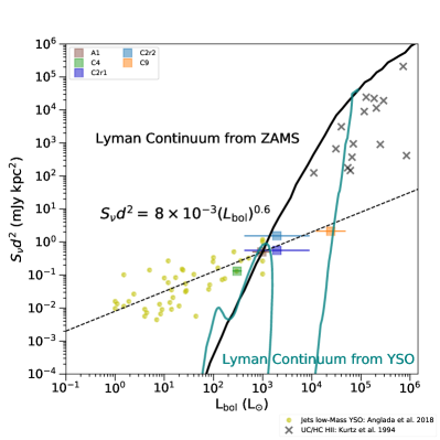
Figure 16: Radio luminosity scaled to 5 GHz (assuming a spectral index $\alpha=0.6$) versus the bolometric luminosity. Note for the two radio sources in C2 we adopt a luminosity value of $L_{\rm bol}$ of C2 divided by 2. The bolometric luminosity is given by the geometric mean value of the isotropic luminosity returned by the valid models for each source. The yellow circles represent ionized jets toward low-mass stars from Anglada (2018). The dashed line shows a power law relation for these sources, given by Anglada et al. (2015): $\left(\frac{S_{\nu}d^{2}}{\rm mJy\>kpc^{2}}\right)=8\times 10^{-3}\left(\frac{L_{\rm bol}}{L_{\odot}}\right)^{0.6}$. The $\times$ symbols are UC and HC HII regions from Kurtz et al. (1994). The black and the cyan continuous lines are the radio emission expected from optically thin H II regions powered by a single zero-age main-sequence (ZAMS) star at a given luminosity (Sánchez-Monge et al. 2013a) and from a YSO with $M_{\rm c}=60~{}M_{\odot}$ and $\Sigma_{\rm cl}=1~{}\rm g~{}cm^{-2}$ (Tanaka et al. 2016), respectively.

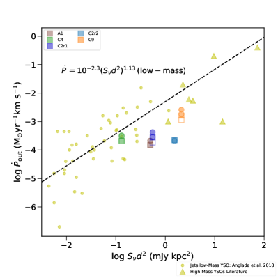
Figure 17: Momentum rate of the molecular outflow as a function of the radio luminosity at 5 GHz. The momentum rate values of the molecular outflow for our sources are measured from our SiO data; for the rest of the data the values are collected from the literature. The symbols for our sources are the same with Figure 13. The yellow circles represent ionized jets associated with low-mass protostars from Anglada et al. (2018). The yellow triangles represent ionized jets associated with high-mass stars (Rodríguez et al. 2008; Moscadelli et al. 2016). The dashed line relation shows the correlation found by Anglada (1995) derived for jets from low-mass stars.

As photoionization cannot account for the observed radio continuum emission of low luminosity objects, shock ionization has been proposed as a viable alternative mechanism (Curiel et al. 1987; González & Cantó 2002) and the correlation of the bolometric and radio luminosities is interpreted as a consequence of the accretion and outflow relationship (Anglada et al. 2018). Additionally, synchrotron emission could also arise from fast shocks in disks and jets (e.g., Carrasco-González et al. 2010). Based on the radio/bolometric luminosity comparison as shown in Figure 16, it seems the radio emission in A1, C2, C4 and C9 is more likely to be from shock ionized radio jets than a HC HII region. Note that for the two radio sources in C2 we adopt a luminosity value of $L_{\rm bol}$ of C2 divided by 2. More information is needed to confirm their nature, such as a robust spectral index derived from multi bands and resolved morphology. If they are shock ionized jets, they are likely to be detected because the cores are massive enough to drive strong shocks. We did not see clear relation between the radio emission detection and $L/M$ and $t_{\rm dyn}/t_{\rm ff}$ (not shown here), which indicate the evolutionary stage. It is likely that our sample is overall at an early stage and photoionization has not become significant enough yet to form a HC HII region, even for the high-mass cores C2 and C9, which would eventually evolve to HII regions based on their current core mass. A similar early-stage population prior to the onset of a HC H II region is also seen in Lim & De Buizer (2019), where half of the 41 MYSO candidates revealed by MIR in W51A have no detected radio continuum emission at centimeter wavelengths. However, we are not sure why other intermediate-mass cores with strong SiO outflows, e.g., the cores in C6, do not show detected shock ionized radio jets.

Also, it has been found previously that the outflow momentum rate is correlated with the radio luminosity, which can be explained by the shock ionization mechanism working in radio jets (Anglada et al. 2018). In particular, the shocked-induced ionization model implies $\left(\frac{S_{\nu}d^{2}}{\rm mJy\,kpc^{2}}\right)=10^{3.5}\eta\left(\frac{\dot{P}}{M_{\odot}\,\rm yr^{-1}\,km\,s^{-1}}\right)$ at $\nu=5$ GHz where $\eta$ is the ionization fraction. In Figure 17 we show the momentum rate ($\dot{P}$) of our SiO molecular outflows that are associated with centimeter emission as a function of the radio luminosity ($S_{\nu}d^{2}$) of the ionized jet estimated from our flux values at 5 GHz. The yellow triangles represent ionized jets associated with high-mass stars as collected from the literature (Rodríguez et al. (2008); Moscadelli et al. (2016)) and the yellow circles represent ionized jets associated with low-mass protostars from Anglada et al. (2018). The molecular outflow data from the literature are from observations using different spectral lines and telescopes, thus the scatter in the data. The outflow momentum rate estimates typically have considerable uncertainties of more than one order of magnitude (Anglada et al. 2018). The dashed line relation in Figure 17 shows the observational correlation found by Anglada (1995) derived for jets associated with low-mass stars with an ionization fraction of $\sim 10\%$. Despite the scatter in the data in Figure 17, our observations appear to suggest that the ionization fraction or the fraction of material that gets ionized by shocks may be higher than $\sim 10\%$ for high-mass protostars than for the low-mass counterpart (see Rosero et al. 2019b for a further discussion). However, a larger and homogeneous sample is required for drawing any conclusions.

If we assume the outflows are materials entrained by jets, there is a higher chance that the radio flux of the jet can be detected in sources that show brighter SiO outflows (see Figure  16 and 17). However, the mm cores associated with detected radio emission are not always the cores that drive the strongest SiO outflows or that have the highest bolometric luminosity (e.g., A1 and C4). Nevertheless, they are among the most massive ones in all the 32 clumps in our ALMA survey. A larger number of detections is required to derive any robust correlation between the radio flux and the core mass, the outflow strength. As discussed in § 4, the detection in our sample is partly limited by sensitivity.

We have a radio detection rate of $\sim$ 27% out of the 15 IRDC clumps with both SiO outflows and 1.3 mm continuum emission. In Rosero et al. (2016) detection rates of radio sources associated with the millimeter dust clumps within IRDCs with and without IR sources (CMC–IRs and CMCs, respectively), and hot molecular cores (HMCs) are 53%, 6%, and 100%, respectively. The majority of our 15 sources should belong to their CMC category. The low detection rate in our sample is consistent with increasing high-mass star formation activity from CMCs to HMCs. The offsets between the 1.3 mm continuum peak and the 6 cm continuum peak are typically $\sim$ 2500 AU, smaller than that of 4000 au and 10000 au for CMC–IRs and HMCs, respectively, in Rosero et al. (2016).

6 Conclusions

In this work, we have presented the results of ALMA observations of SiO(5-4) and VLA 6 cm radio observations made towards 32 IRDC clumps potentially harboring prestellar/protostellar sources. Our goal is to characterize a large number of protostars from low-mass to high-mass at the earliest phases with their outflow emission, and investigate the onset of SiO emission as shock tracers and the onset of ionization, to understand massive star formation. In summary, our main results and conclusions are as follows.

1. We have detected SiO(5-4) emission in 20 out of 32 IRDC clumps with a detection rate of 62%. From the non-detection in our sample and comparison with the SiO detection rate in other IR-dark clumps, it seems that at early evolutionary stages, shocked gas is more common in the higher mass regime. Compared with more evolved IR-bright protostars, the SiO detection rate is overall higher in early-stage protostars. Compared with CO outflows, which are generally highly collimated, the SiO outflows appear to be somewhat more disordered and fragmented, though most are still consistent with being collimated structures or parts of the collimated outflows.

2. In the 20 sources with detected SiO, 11 sources with relatively strong SiO emission seem to host SiO outflows based on their wide line widths. Most SiO outflows show bipolar structures though they can be highly asymmetric. Some SiO outflows are collimated while others are less ordered. There is evidence for successive ejection events as well as multiple outflows originating from $\lesssim$ 0.1pc, which can be due to outflow changing orientation over time. For the six protostellar sources with strongest SiO outflow emission, we do not see clear dependence of the collimation of the outflows on evolutionary stage.

3. For the six protostars with strongest SiO emission, we locate the protostellar sources driving the outflows, which appear as nearby mm continuum peaks, in position-velocity space utilizing dense gas tracers DCN(3-2), DCO⁺(3-2) and C¹⁸O(2-1). They have relatively low outflow masses, mass outflow rates and momentum flow rates, in spite of the fact that some of them are high-mass protostellar candidates based on their mm core masses. The outflow masses appear to increase with the core mass. We do not see a strong dependence of mechanical force and mass entrainment rate on bolometric luminosity.

4. Where there is SiO(5-4) emission seen, we can always find 1.3 mm continuum emission and some infrared emission nearby, but not vice versa. The low luminosity, low accretion rates and low current stellar mass returned by SED fitting suggest the sources in our sample are at an early evolutionary stage. With the entire sample and data from literature, we see a slight increasing trend of SiO line luminosity with the bolometric luminosity, which suggests more powerful shocks in the vicinity of more massive YSOs. We do not see clear relation between the SiO luminosity and the evolutionary stage indicated by $L/M$. Given the fact that most of our sample have SiO detection, it seems that as long as a protostar approaches a luminosity of $\sim\ 10^{2}\ L_{\odot}$, the shocks in the outflow are strong enough to form SiO emission.

5. We detect 6 cm radio continuum emission in 4 out of the 15 sources with bright SiO emission. The radio emission is likely due to shock-ionized jets associated with most massive protostellar cores. It is likely that our sample is overall at an early stage and photoionization has not become significant enough yet to form HC HII regions, even for the high-mass cores. Our VLA detections are limited by sensitivity and higher-sensitivity observations are needed to find a larger number of sources to be able to determine if there is any robust correlation between the radio flux and the core mass, outflow strength and evolutionary stage.

6. As an overall summary of implications for massive star formation, we conclude that SiO outflows and radio continuum emission are important diagnostic tracers of sources that have relatively special shock conditions that often have properties consistent with being massive protostars in an early stage of evolution. While the SiO emission is generally more disordered and/or sparse than that seen in CO, the emission features are generally consistent with being parts of highly collimated outflows. This indicates that these candidate early-stage massive protostars are launching such outflows, which is an expectation of core accretion models. Among our sample of six strong SiO outflow sources, we have one example, C9, that exhibits a much more disordered morphology, which may indicate a different type of outflow or the presence of multiple protostars in a small projected region of the sky that are each launching collimated SiO outflows. Higher resolution follow-up observations of this source are needed to distinguish these possibilities.

Appendix A MIR Photometry and SED fitting

We used PHOTUTILS (https://doi.org/10.5281/zenodo.596036), a PYTHON package to measure the flux density of the entire sample. Note that clumps with neither 1.3 mm continuum nor SiO emission are not taken into consideration. The circular aperture is determined based on the 70 $\mu$m and 160 $\mu$m 2D profile to cover most of the clumpy infrared emission. Sometimes when the boundary of the core and the background is unclear, we adopt an aperture radius of 15″, so that the aperture diameter is close to the beam size of Herschel 500 $\mu$m images. The aperture radii for most sources are around 15″. After measuring the flux inside the aperture, we carry out background subtraction using the median flux density in an annular region extending from 1 to 2 aperture radii to remove general background and foreground contamination and the effect of a cooler, more massive clump surrounding the core at long wavelengths (see also De Buizer et al. 2017; Liu et al. 2019, 2020; Moser et al. 2020). Note that if the annular region overlaps with the apertures of other sources, we exclude the overlapping part for background estimation. The error of the flux is estimated to be the quadratic sum of the 10% of the background subtracted flux as calibration uncertainty and the background fluctuation. The background fluctuation is derived in the following way: first we divide the annular region extending from 1 to 2 aperture radii evenly into six sectors and measure the standard deviation of the mean values in the six sectors; then we rotate every sector by 10°and measure the standard deviation in the same way again; we repeat the rotation for another four times and obtain six measured standard deviations in total; finally we derive the mean value of the six standard deviation as the estimation of the background fluctuation.

We use data at wavelengths $<\ 8\ \mu$m as upper limits due to PAH emission and thermal emission from very small grains. Additionally, if the background is stronger than the flux density inside the aperture, then the flux density without background subtraction is given and treated as an upper limit. The fitting procedure involves convolving model SEDs with the filter response functions for the various telescope bands. Source distances were adopted from Butler & Tan (2012).

We show the SED fitting of other sources in the sample in Figure 18. The model parameters are listed in Table 6.

Table 6: Parameters of the Ten Best Fitted Models

Source	$\chi^{2}$/N	$M_{\rm c}$	$\Sigma_{\rm cl}$	$R_{core}$	$m_{*}$	$\theta_{\rm view}$	$A_{V}$	$M_{\rm env}$	$\theta_{w,\rm esc}$	$\dot{M}_{\rm disk}$	$L_{\rm bol,iso}$	$L_{\rm bol}$
		($M_{\odot}$)	(g $\rm cm^{-2}$)	(pc) ($\arcsec$)	($M_{\odot}$)	(deg)	(mag)	($M_{\odot}$)	(deg)	($M_{\odot}$/yr)	($L_{\odot}$)	($L_{\odot}$)
A1	0.16	480	0.1	0.51 ( 22 )	2.0	48	1000.0	477	4	4.3$\times 10^{-5}$	5.7$\times 10^{2}$	5.7$\times 10^{2}$
$d$ = 4.8 kpc	0.19	400	0.1	0.47 ( 20 )	2.0	13	941.9	391	4	4.1$\times 10^{-5}$	7.7$\times 10^{2}$	5.5$\times 10^{2}$
$R_{ap}$ = 16 ″	0.22	240	0.1	0.36 ( 15 )	4.0	77	1000.0	229	9	5.1$\times 10^{-5}$	9.1$\times 10^{2}$	1.0$\times 10^{3}$
= 0.37 pc	0.24	320	0.1	0.42 ( 18 )	4.0	13	656.7	308	7	5.5$\times 10^{-5}$	1.2$\times 10^{3}$	5.4$\times 10^{2}$
	0.26	200	0.3	0.19 ( 8 )	1.0	29	1000.0	196	4	5.8$\times 10^{-5}$	5.2$\times 10^{2}$	5.2$\times 10^{2}$
	0.29	400	0.1	0.47 ( 20 )	4.0	89	1000.0	390	7	5.8$\times 10^{-5}$	9.4$\times 10^{2}$	1.0$\times 10^{3}$
	0.33	200	0.1	0.33 ( 14 )	4.0	13	682.7	194	10	4.8$\times 10^{-5}$	1.9$\times 10^{3}$	6.7$\times 10^{2}$
	0.33	160	0.1	0.29 ( 13 )	4.0	13	1000.0	151	12	4.5$\times 10^{-5}$	3.1$\times 10^{3}$	9.1$\times 10^{2}$
	0.35	480	0.1	0.51 ( 22 )	4.0	89	1000.0	474	6	6.1$\times 10^{-5}$	9.2$\times 10^{2}$	1.0$\times 10^{3}$
	0.36	240	0.1	0.36 ( 15 )	2.0	29	411.4	233	6	3.6$\times 10^{-5}$	5.2$\times 10^{2}$	5.2$\times 10^{2}$
Averages	0.26	291	0.1	0.37 ( 16 )	2.8	41	869.3	283	7	4.9$\times 10^{-5}$	9.6$\times 10^{2}$	7.0$\times 10^{2}$
A2	0.53	160	0.1	0.29 ( 13 )	2.0	65	1000.0	156	8	3.3$\times 10^{-5}$	4.0$\times 10^{2}$	4.3$\times 10^{2}$
$d$ = 4.8 kpc	0.54	200	0.1	0.33 ( 14 )	2.0	74	1000.0	194	7	3.5$\times 10^{-5}$	3.2$\times 10^{2}$	3.5$\times 10^{2}$
$R_{ap}$ = 16 ″	0.54	100	0.1	0.23 ( 10 )	4.0	83	1000.0	91	15	4.0$\times 10^{-5}$	6.6$\times 10^{2}$	8.8$\times 10^{2}$
= 0.37 pc	0.56	100	0.3	0.13 ( 6 )	1.0	86	1000.0	97	6	4.9$\times 10^{-5}$	4.2$\times 10^{2}$	4.4$\times 10^{2}$
	0.57	120	0.1	0.25 ( 11 )	4.0	89	1000.0	111	14	4.2$\times 10^{-5}$	7.3$\times 10^{2}$	9.4$\times 10^{2}$
	0.57	80	0.3	0.12 ( 5 )	2.0	77	1000.0	76	11	6.4$\times 10^{-5}$	5.3$\times 10^{2}$	6.2$\times 10^{2}$
	0.57	120	0.1	0.25 ( 11 )	2.0	22	915.9	117	9	3.0$\times 10^{-5}$	4.3$\times 10^{2}$	4.3$\times 10^{2}$
	0.58	80	0.1	0.21 ( 9 )	4.0	22	1000.0	71	18	3.7$\times 10^{-5}$	9.0$\times 10^{2}$	8.5$\times 10^{2}$
	0.60	60	1.0	0.06 ( 2 )	0.5	89	1000.0	59	5	7.2$\times 10^{-5}$	3.9$\times 10^{2}$	4.0$\times 10^{2}$
	0.60	50	1.0	0.05 ( 2 )	0.5	29	1000.0	50	5	6.9$\times 10^{-5}$	3.9$\times 10^{2}$	4.0$\times 10^{2}$
Averages	0.57	99	0.2	0.16 ( 7 )	1.7	64	991.6	94	10	4.5$\times 10^{-5}$	4.9$\times 10^{2}$	5.4$\times 10^{2}$
A3	0.94	320	0.1	0.42 ( 18 )	2.0	13	1000.0	315	5	3.9$\times 10^{-5}$	5.9$\times 10^{2}$	3.8$\times 10^{2}$
$d$ = 4.8 kpc	0.99	320	0.1	0.42 ( 18 )	4.0	89	1000.0	308	7	5.5$\times 10^{-5}$	4.9$\times 10^{2}$	5.4$\times 10^{2}$
$R_{ap}$ = 16 ″	1.09	240	0.1	0.36 ( 15 )	2.0	71	1000.0	233	6	3.6$\times 10^{-5}$	4.9$\times 10^{2}$	5.2$\times 10^{2}$
= 0.37 pc	1.21	200	0.1	0.33 ( 14 )	4.0	89	1000.0	194	10	4.8$\times 10^{-5}$	5.7$\times 10^{2}$	6.7$\times 10^{2}$
	1.30	400	0.1	0.47 ( 20 )	2.0	89	1000.0	391	4	4.1$\times 10^{-5}$	5.3$\times 10^{2}$	5.5$\times 10^{2}$
	1.59	160	0.1	0.29 ( 13 )	4.0	86	1000.0	151	12	4.5$\times 10^{-5}$	7.4$\times 10^{2}$	9.1$\times 10^{2}$
	1.60	200	0.1	0.33 ( 14 )	2.0	13	770.8	194	7	3.5$\times 10^{-5}$	7.3$\times 10^{2}$	3.5$\times 10^{2}$
	1.62	160	0.1	0.29 ( 13 )	2.0	13	1000.0	156	8	3.3$\times 10^{-5}$	1.0$\times 10^{3}$	4.3$\times 10^{2}$
	1.62	480	0.1	0.51 ( 22 )	2.0	89	1000.0	477	4	4.3$\times 10^{-5}$	5.5$\times 10^{2}$	5.7$\times 10^{2}$
	1.69	120	0.1	0.25 ( 11 )	4.0	39	1000.0	111	14	4.2$\times 10^{-5}$	8.4$\times 10^{2}$	9.4$\times 10^{2}$
Averages	1.33	238	0.1	0.36 ( 15 )	2.6	59	977.1	230	8	4.1$\times 10^{-5}$	6.4$\times 10^{2}$	5.6$\times 10^{2}$
C4	0.97	320	0.1	0.42 ( 17 )	1.0	44	1000.0	315	3	2.8$\times 10^{-5}$	2.0$\times 10^{2}$	2.0$\times 10^{2}$
$d$ = 5.0 kpc	0.98	240	0.1	0.36 ( 15 )	1.0	48	1000.0	240	4	2.6$\times 10^{-5}$	2.4$\times 10^{2}$	2.4$\times 10^{2}$
$R_{ap}$ = 13 ″	1.10	200	0.1	0.33 ( 14 )	2.0	89	1000.0	194	7	3.5$\times 10^{-5}$	3.2$\times 10^{2}$	3.5$\times 10^{2}$
= 0.32 pc	1.19	200	0.1	0.33 ( 14 )	1.0	13	767.8	197	4	2.5$\times 10^{-5}$	2.7$\times 10^{2}$	1.8$\times 10^{2}$
	1.19	100	0.1	0.23 ( 10 )	2.0	44	1000.0	97	11	2.9$\times 10^{-5}$	3.5$\times 10^{2}$	3.8$\times 10^{2}$
	1.22	120	0.1	0.25 ( 11 )	2.0	80	1000.0	117	9	3.0$\times 10^{-5}$	3.7$\times 10^{2}$	4.3$\times 10^{2}$
	1.23	160	0.1	0.29 ( 12 )	1.0	22	828.8	156	5	2.3$\times 10^{-5}$	2.1$\times 10^{2}$	2.0$\times 10^{2}$
	1.28	160	0.1	0.29 ( 12 )	2.0	86	1000.0	156	8	3.3$\times 10^{-5}$	3.9$\times 10^{2}$	4.3$\times 10^{2}$
	1.32	120	0.1	0.25 ( 11 )	1.0	13	840.8	120	6	2.2$\times 10^{-5}$	4.3$\times 10^{2}$	2.2$\times 10^{2}$
	1.34	80	0.1	0.21 ( 9 )	2.0	22	1000.0	75	12	2.7$\times 10^{-5}$	3.5$\times 10^{2}$	3.5$\times 10^{2}$
Averages	1.18	157	0.1	0.29 ( 12 )	1.4	46	943.7	153	7	2.7$\times 10^{-5}$	3.0$\times 10^{2}$	2.8$\times 10^{2}$
C5	0.02	240	0.1	0.36 ( 15 )	1.0	83	409.4	240	4	2.6$\times 10^{-5}$	2.3$\times 10^{2}$	2.4$\times 10^{2}$
$d$ = 5.0 kpc	0.02	120	0.1	0.25 ( 11 )	2.0	22	1000.0	117	9	3.0$\times 10^{-5}$	4.3$\times 10^{2}$	4.3$\times 10^{2}$
$R_{ap}$ = 15 ″	0.02	320	0.1	0.42 ( 17 )	1.0	89	241.2	315	3	2.8$\times 10^{-5}$	1.9$\times 10^{2}$	2.0$\times 10^{2}$
= 0.36 pc	0.02	200	0.1	0.33 ( 14 )	2.0	86	1000.0	194	7	3.5$\times 10^{-5}$	3.2$\times 10^{2}$	3.5$\times 10^{2}$
	0.02	160	0.1	0.29 ( 12 )	2.0	89	1000.0	156	8	3.3$\times 10^{-5}$	3.9$\times 10^{2}$	4.3$\times 10^{2}$
	0.03	100	0.3	0.13 ( 5 )	32.0	55	1000.0	4	81	5.0$\times 10^{-5}$	1.7$\times 10^{5}$	1.4$\times 10^{5}$
	0.03	100	0.3	0.13 ( 5 )	0.5	44	651.7	99	4	3.5$\times 10^{-5}$	2.4$\times 10^{2}$	2.4$\times 10^{2}$
	0.03	60	0.1	0.18 ( 7 )	16.0	13	207.2	7	76	2.0$\times 10^{-5}$	5.3$\times 10^{4}$	2.5$\times 10^{4}$
	0.03	80	0.1	0.21 ( 9 )	4.0	22	1000.0	71	18	3.7$\times 10^{-5}$	9.0$\times 10^{2}$	8.5$\times 10^{2}$
	0.03	100	0.1	0.23 ( 10 )	2.0	13	115.1	97	11	2.9$\times 10^{-5}$	1.2$\times 10^{3}$	3.8$\times 10^{2}$
Averages	0.02	130	0.1	0.24 ( 10 )	2.6	51	662.5	75	22	3.1$\times 10^{-5}$	1.2$\times 10^{3}$	9.9$\times 10^{2}$
C7	0.08	200	0.1	0.33 ( 14 )	0.5	22	1000.0	200	3	1.7$\times 10^{-5}$	1.3$\times 10^{2}$	1.3$\times 10^{2}$
$d$ = 5.0 kpc	0.09	160	0.1	0.29 ( 12 )	1.0	89	1000.0	156	5	2.3$\times 10^{-5}$	1.9$\times 10^{2}$	2.0$\times 10^{2}$
$R_{ap}$ = 15 ″	0.10	120	0.1	0.25 ( 11 )	1.0	80	1000.0	120	6	2.2$\times 10^{-5}$	2.0$\times 10^{2}$	2.2$\times 10^{2}$
= 0.36 pc	0.10	200	0.1	0.33 ( 14 )	1.0	86	1000.0	197	4	2.5$\times 10^{-5}$	1.7$\times 10^{2}$	1.8$\times 10^{2}$
	0.11	100	0.1	0.23 ( 10 )	1.0	13	1000.0	98	7	2.0$\times 10^{-5}$	4.4$\times 10^{2}$	2.0$\times 10^{2}$
	0.13	60	0.1	0.18 ( 7 )	16.0	51	1000.0	7	76	2.0$\times 10^{-5}$	3.4$\times 10^{4}$	2.5$\times 10^{4}$
	0.13	80	0.1	0.21 ( 9 )	2.0	48	1000.0	75	12	2.7$\times 10^{-5}$	3.1$\times 10^{2}$	3.5$\times 10^{2}$
	0.16	100	0.1	0.23 ( 10 )	2.0	89	1000.0	97	11	2.9$\times 10^{-5}$	3.2$\times 10^{2}$	3.8$\times 10^{2}$
	0.16	60	0.1	0.18 ( 7 )	2.0	22	1000.0	55	15	2.5$\times 10^{-5}$	3.5$\times 10^{2}$	3.5$\times 10^{2}$
	0.17	160	0.1	0.29 ( 12 )	0.5	13	0.0	158	3	1.6$\times 10^{-5}$	1.2$\times 10^{2}$	9.8$\times 10^{1}$
Averages	0.12	113	0.1	0.25 ( 10 )	1.4	51	900.0	89	14	2.2$\times 10^{-5}$	3.8$\times 10^{2}$	3.5$\times 10^{2}$
C8	0.17	100	0.3	0.13 ( 5 )	32.0	74	997.0	4	81	5.0$\times 10^{-5}$	5.3$\times 10^{4}$	1.4$\times 10^{5}$
$d$ = 5.0 kpc	0.18	60	0.1	0.18 ( 7 )	2.0	86	632.6	55	15	2.5$\times 10^{-5}$	2.6$\times 10^{2}$	3.5$\times 10^{2}$
$R_{ap}$ = 15 ″	0.18	50	0.1	0.16 ( 7 )	4.0	89	1000.0	41	24	3.2$\times 10^{-5}$	4.7$\times 10^{2}$	7.9$\times 10^{2}$
= 0.36 pc	0.18	50	0.3	0.09 ( 4 )	0.5	80	538.5	48	6	2.9$\times 10^{-5}$	1.8$\times 10^{2}$	1.9$\times 10^{2}$
	0.18	80	0.1	0.21 ( 9 )	1.0	83	0.0	77	8	1.9$\times 10^{-5}$	1.7$\times 10^{2}$	1.9$\times 10^{2}$
	0.19	60	0.3	0.10 ( 4 )	0.5	77	1000.0	60	5	3.0$\times 10^{-5}$	1.8$\times 10^{2}$	1.8$\times 10^{2}$
	0.19	30	0.3	0.07 ( 3 )	1.0	34	697.7	28	13	3.5$\times 10^{-5}$	3.5$\times 10^{2}$	4.3$\times 10^{2}$
	0.19	30	0.3	0.07 ( 3 )	2.0	13	873.9	26	21	4.8$\times 10^{-5}$	4.0$\times 10^{3}$	6.2$\times 10^{2}$
	0.19	40	0.1	0.15 ( 6 )	4.0	44	219.2	30	27	3.0$\times 10^{-5}$	5.1$\times 10^{2}$	7.5$\times 10^{2}$
	0.19	50	0.1	0.16 ( 7 )	2.0	22	26.0	46	16	2.4$\times 10^{-5}$	3.1$\times 10^{2}$	3.1$\times 10^{2}$
Averages	0.18	51	0.2	0.13 ( 5 )	2.0	60	598.5	34	22	3.1$\times 10^{-5}$	6.1$\times 10^{2}$	6.6$\times 10^{2}$
D1	0.29	320	0.1	0.42 ( 15 )	1.0	22	1000.0	315	3	2.8$\times 10^{-5}$	2.1$\times 10^{2}$	2.0$\times 10^{2}$
$d$ = 5.7 kpc	0.30	200	0.1	0.33 ( 12 )	2.0	34	1000.0	194	7	3.5$\times 10^{-5}$	3.5$\times 10^{2}$	3.5$\times 10^{2}$
$R_{ap}$ = 15 ″	0.31	240	0.1	0.36 ( 13 )	1.0	13	1000.0	240	4	2.6$\times 10^{-5}$	3.2$\times 10^{2}$	2.4$\times 10^{2}$
= 0.41 pc	0.32	160	0.1	0.29 ( 11 )	2.0	48	1000.0	156	8	3.3$\times 10^{-5}$	4.1$\times 10^{2}$	4.3$\times 10^{2}$
	0.33	320	0.1	0.42 ( 15 )	2.0	89	1000.0	315	5	3.9$\times 10^{-5}$	3.6$\times 10^{2}$	3.8$\times 10^{2}$
	0.35	120	0.1	0.25 ( 9 )	2.0	22	1000.0	117	9	3.0$\times 10^{-5}$	4.3$\times 10^{2}$	4.3$\times 10^{2}$
	0.37	240	0.1	0.36 ( 13 )	2.0	89	1000.0	233	6	3.6$\times 10^{-5}$	4.8$\times 10^{2}$	5.2$\times 10^{2}$
	0.38	200	0.1	0.33 ( 12 )	4.0	89	1000.0	194	10	4.8$\times 10^{-5}$	5.7$\times 10^{2}$	6.7$\times 10^{2}$
	0.38	100	0.1	0.23 ( 8 )	4.0	34	1000.0	91	15	4.0$\times 10^{-5}$	7.8$\times 10^{2}$	8.8$\times 10^{2}$
	0.39	120	0.1	0.25 ( 9 )	4.0	89	1000.0	111	14	4.2$\times 10^{-5}$	7.3$\times 10^{2}$	9.4$\times 10^{2}$
Averages	0.34	188	0.1	0.32 ( 12 )	2.1	53	1000.0	181	8	3.5$\times 10^{-5}$	4.3$\times 10^{2}$	4.5$\times 10^{2}$
D3	0.61	400	0.1	0.47 ( 17 )	2.0	68	1000.0	391	4	4.1$\times 10^{-5}$	5.3$\times 10^{2}$	5.5$\times 10^{2}$
$d$ = 5.7 kpc	0.62	480	0.1	0.51 ( 18 )	2.0	89	1000.0	477	4	4.3$\times 10^{-5}$	5.5$\times 10^{2}$	5.7$\times 10^{2}$
$R_{ap}$ = 15 ″	0.62	320	0.1	0.42 ( 15 )	4.0	39	1000.0	308	7	5.5$\times 10^{-5}$	5.3$\times 10^{2}$	5.4$\times 10^{2}$
= 0.41 pc	0.75	320	0.1	0.42 ( 15 )	2.0	13	1000.0	315	5	3.9$\times 10^{-5}$	5.9$\times 10^{2}$	3.8$\times 10^{2}$
	0.76	240	0.1	0.36 ( 13 )	2.0	29	1000.0	233	6	3.6$\times 10^{-5}$	5.2$\times 10^{2}$	5.2$\times 10^{2}$
	0.78	200	0.1	0.33 ( 12 )	4.0	29	1000.0	194	10	4.8$\times 10^{-5}$	6.5$\times 10^{2}$	6.7$\times 10^{2}$
	0.90	320	0.3	0.23 ( 8 )	96.0	74	1000.0	7	85	6.6$\times 10^{-5}$	9.5$\times 10^{5}$	1.2$\times 10^{6}$
	0.91	160	0.1	0.29 ( 11 )	4.0	29	1000.0	151	12	4.5$\times 10^{-5}$	8.6$\times 10^{2}$	9.1$\times 10^{2}$
	0.93	240	0.1	0.36 ( 13 )	4.0	86	1000.0	229	9	5.1$\times 10^{-5}$	9.0$\times 10^{2}$	1.0$\times 10^{3}$
	0.95	200	0.3	0.19 ( 7 )	1.0	80	1000.0	196	4	5.8$\times 10^{-5}$	5.1$\times 10^{2}$	5.2$\times 10^{2}$
Averages	0.77	273	0.1	0.34 ( 12 )	3.6	54	1000.0	180	15	4.8$\times 10^{-5}$	1.3$\times 10^{3}$	1.3$\times 10^{3}$
D5	0.32	320	0.1	0.42 ( 15 )	4.0	39	1000.0	308	7	5.5$\times 10^{-5}$	5.3$\times 10^{2}$	5.4$\times 10^{2}$
$d$ = 5.7 kpc	0.33	400	0.1	0.47 ( 17 )	2.0	83	1000.0	391	4	4.1$\times 10^{-5}$	5.3$\times 10^{2}$	5.5$\times 10^{2}$
$R_{ap}$ = 11 ″	0.40	480	0.1	0.51 ( 18 )	2.0	89	1000.0	477	4	4.3$\times 10^{-5}$	5.5$\times 10^{2}$	5.7$\times 10^{2}$
= 0.30 pc	0.45	200	0.1	0.33 ( 12 )	4.0	13	1000.0	194	10	4.8$\times 10^{-5}$	1.9$\times 10^{3}$	6.7$\times 10^{2}$
	0.46	240	0.1	0.36 ( 13 )	2.0	29	1000.0	233	6	3.6$\times 10^{-5}$	5.2$\times 10^{2}$	5.2$\times 10^{2}$
	0.47	320	0.1	0.42 ( 15 )	2.0	13	775.8	315	5	3.9$\times 10^{-5}$	5.9$\times 10^{2}$	3.8$\times 10^{2}$
	0.51	200	0.3	0.19 ( 7 )	1.0	71	1000.0	196	4	5.8$\times 10^{-5}$	5.1$\times 10^{2}$	5.2$\times 10^{2}$
	0.51	160	0.1	0.29 ( 11 )	4.0	22	1000.0	151	12	4.5$\times 10^{-5}$	9.0$\times 10^{2}$	9.1$\times 10^{2}$
	0.54	240	0.1	0.36 ( 13 )	4.0	89	1000.0	229	9	5.1$\times 10^{-5}$	9.0$\times 10^{2}$	1.0$\times 10^{3}$
	0.55	100	0.3	0.13 ( 5 )	32.0	13	1000.0	4	81	5.0$\times 10^{-5}$	3.0$\times 10^{5}$	1.4$\times 10^{5}$
Averages	0.45	243	0.1	0.32 ( 12 )	3.2	46	977.6	174	14	4.6$\times 10^{-5}$	1.3$\times 10^{3}$	1.0$\times 10^{3}$
D6	0.03	320	0.1	0.42 ( 15 )	2.0	13	240.2	315	5	3.9$\times 10^{-5}$	5.9$\times 10^{2}$	3.8$\times 10^{2}$
$d$ = 5.7 kpc	0.03	200	0.1	0.33 ( 12 )	2.0	22	200.2	194	7	3.5$\times 10^{-5}$	3.6$\times 10^{2}$	3.5$\times 10^{2}$
$R_{ap}$ = 15 ″	0.03	160	0.1	0.29 ( 11 )	2.0	13	294.3	156	8	3.3$\times 10^{-5}$	1.0$\times 10^{3}$	4.3$\times 10^{2}$
= 0.41 pc	0.03	320	0.3	0.23 ( 8 )	96.0	83	521.5	7	85	6.6$\times 10^{-5}$	1.5$\times 10^{4}$	1.2$\times 10^{6}$
	0.03	120	0.1	0.25 ( 9 )	2.0	22	239.2	117	9	3.0$\times 10^{-5}$	4.3$\times 10^{2}$	4.3$\times 10^{2}$
	0.04	240	0.1	0.36 ( 13 )	1.0	22	130.1	240	4	2.6$\times 10^{-5}$	2.4$\times 10^{2}$	2.4$\times 10^{2}$
	0.04	100	0.3	0.13 ( 5 )	32.0	55	495.5	4	81	5.0$\times 10^{-5}$	1.7$\times 10^{5}$	1.4$\times 10^{5}$
	0.04	100	0.3	0.13 ( 5 )	0.5	13	43.0	99	4	3.5$\times 10^{-5}$	3.1$\times 10^{2}$	2.4$\times 10^{2}$
	0.04	320	0.1	0.42 ( 15 )	1.0	22	95.1	315	3	2.8$\times 10^{-5}$	2.1$\times 10^{2}$	2.0$\times 10^{2}$
	0.04	80	0.1	0.21 ( 8 )	4.0	13	428.4	71	18	3.7$\times 10^{-5}$	4.4$\times 10^{3}$	8.5$\times 10^{2}$
Averages	0.03	173	0.1	0.26 ( 9 )	3.2	28	268.8	84	22	3.6$\times 10^{-5}$	1.3$\times 10^{3}$	1.5$\times 10^{3}$
D8	0.07	240	0.1	0.36 ( 13 )	2.0	80	1000.0	233	6	3.6$\times 10^{-5}$	4.8$\times 10^{2}$	5.2$\times 10^{2}$
$d$ = 5.7 kpc	0.07	100	0.3	0.13 ( 5 )	1.0	89	1000.0	97	6	4.9$\times 10^{-5}$	4.2$\times 10^{2}$	4.4$\times 10^{2}$
$R_{ap}$ = 11 ″	0.07	320	0.1	0.42 ( 15 )	4.0	89	1000.0	308	7	5.5$\times 10^{-5}$	4.9$\times 10^{2}$	5.4$\times 10^{2}$
= 0.30 pc	0.08	200	0.1	0.33 ( 12 )	4.0	89	1000.0	194	10	4.8$\times 10^{-5}$	5.7$\times 10^{2}$	6.7$\times 10^{2}$
	0.08	60	0.3	0.10 ( 4 )	1.0	62	1000.0	58	8	4.3$\times 10^{-5}$	4.2$\times 10^{2}$	4.7$\times 10^{2}$
	0.09	30	1.0	0.04 ( 1 )	0.5	80	1000.0	29	8	6.0$\times 10^{-5}$	3.8$\times 10^{2}$	4.2$\times 10^{2}$
	0.09	80	0.3	0.12 ( 4 )	1.0	34	936.9	79	7	4.6$\times 10^{-5}$	3.3$\times 10^{2}$	3.5$\times 10^{2}$
	0.10	100	0.1	0.23 ( 8 )	4.0	77	1000.0	91	15	4.0$\times 10^{-5}$	6.6$\times 10^{2}$	8.8$\times 10^{2}$
	0.11	20	1.0	0.03 ( 1 )	0.5	71	1000.0	19	10	5.4$\times 10^{-5}$	3.7$\times 10^{2}$	4.5$\times 10^{2}$
	0.12	40	1.0	0.05 ( 2 )	0.5	86	1000.0	39	6	6.5$\times 10^{-5}$	3.8$\times 10^{2}$	4.0$\times 10^{2}$
Averages	0.09	84	0.3	0.13 ( 5 )	1.3	76	993.7	81	8	4.9$\times 10^{-5}$	4.4$\times 10^{2}$	4.9$\times 10^{2}$
D9	0.24	200	0.1	0.33 ( 12 )	0.5	13	189.2	200	3	1.7$\times 10^{-5}$	1.5$\times 10^{2}$	1.3$\times 10^{2}$
$d$ = 5.7 kpc	0.29	100	0.1	0.23 ( 8 )	1.0	13	453.5	98	7	2.0$\times 10^{-5}$	4.4$\times 10^{2}$	2.0$\times 10^{2}$
$R_{ap}$ = 12 ″	0.30	80	0.1	0.21 ( 8 )	1.0	13	354.4	77	8	1.9$\times 10^{-5}$	4.6$\times 10^{2}$	1.9$\times 10^{2}$
= 0.33 pc	0.33	200	0.1	0.33 ( 12 )	1.0	89	479.5	197	4	2.5$\times 10^{-5}$	1.7$\times 10^{2}$	1.8$\times 10^{2}$
	0.35	160	0.1	0.29 ( 11 )	1.0	89	597.6	156	5	2.3$\times 10^{-5}$	1.9$\times 10^{2}$	2.0$\times 10^{2}$
	0.36	120	0.1	0.25 ( 9 )	1.0	13	698.7	120	6	2.2$\times 10^{-5}$	4.3$\times 10^{2}$	2.2$\times 10^{2}$
	0.36	60	0.1	0.18 ( 7 )	1.0	13	344.3	57	10	1.8$\times 10^{-5}$	6.1$\times 10^{2}$	2.0$\times 10^{2}$
	0.38	50	0.1	0.16 ( 6 )	2.0	13	508.5	46	16	2.4$\times 10^{-5}$	1.6$\times 10^{3}$	3.1$\times 10^{2}$
	0.42	60	0.1	0.18 ( 7 )	2.0	13	849.8	55	15	2.5$\times 10^{-5}$	1.7$\times 10^{3}$	3.5$\times 10^{2}$
	0.45	80	0.1	0.21 ( 8 )	2.0	89	1000.0	75	12	2.7$\times 10^{-5}$	2.8$\times 10^{2}$	3.5$\times 10^{2}$
Averages	0.34	99	0.1	0.23 ( 8 )	1.1	36	547.5	95	9	2.2$\times 10^{-5}$	4.3$\times 10^{2}$	2.2$\times 10^{2}$
E1	0.21	30	0.1	0.13 ( 5 )	2.0	86	466.5	25	23	2.0$\times 10^{-5}$	1.4$\times 10^{2}$	2.4$\times 10^{2}$
$d$ = 5.1 kpc	0.21	30	0.1	0.13 ( 5 )	1.0	86	599.6	27	15	1.5$\times 10^{-5}$	1.3$\times 10^{2}$	1.7$\times 10^{2}$
$R_{ap}$ = 15 ″	0.22	80	1.0	0.07 ( 3 )	32.0	83	709.7	3	79	1.4$\times 10^{-4}$	2.1$\times 10^{3}$	1.6$\times 10^{5}$
= 0.37 pc	0.22	20	0.3	0.06 ( 2 )	4.0	89	1000.0	11	38	5.4$\times 10^{-5}$	3.1$\times 10^{2}$	1.1$\times 10^{3}$
	0.22	30	0.1	0.13 ( 5 )	8.0	86	1000.0	9	57	2.6$\times 10^{-5}$	7.5$\times 10^{2}$	6.3$\times 10^{3}$
	0.23	60	0.1	0.18 ( 7 )	16.0	83	348.3	7	76	2.0$\times 10^{-5}$	6.5$\times 10^{2}$	2.5$\times 10^{4}$
	0.23	40	0.1	0.15 ( 6 )	0.5	58	0.0	39	8	1.1$\times 10^{-5}$	8.1$\times 10^{1}$	8.8$\times 10^{1}$
	0.23	50	0.1	0.16 ( 7 )	0.5	77	230.2	49	7	1.2$\times 10^{-5}$	7.9$\times 10^{1}$	8.7$\times 10^{1}$
	0.24	40	0.1	0.15 ( 6 )	1.0	89	1000.0	38	12	1.6$\times 10^{-5}$	1.3$\times 10^{2}$	1.7$\times 10^{2}$
	0.24	20	0.3	0.06 ( 2 )	2.0	89	1000.0	15	27	4.2$\times 10^{-5}$	2.2$\times 10^{2}$	4.8$\times 10^{2}$
Averages	0.23	36	0.2	0.11 ( 5 )	2.6	82	635.4	16	34	2.6$\times 10^{-5}$	2.5$\times 10^{2}$	9.6$\times 10^{2}$
E2	0.13	30	0.3	0.07 ( 3 )	2.0	86	1000.0	26	21	4.8$\times 10^{-5}$	3.7$\times 10^{2}$	6.2$\times 10^{2}$
$d$ = 5.1 kpc	0.14	30	0.3	0.07 ( 3 )	1.0	86	1000.0	28	13	3.5$\times 10^{-5}$	3.3$\times 10^{2}$	4.3$\times 10^{2}$
$R_{ap}$ = 15 ″	0.14	40	0.3	0.08 ( 3 )	0.5	22	886.9	39	7	2.7$\times 10^{-5}$	1.8$\times 10^{2}$	1.9$\times 10^{2}$
= 0.37 pc	0.14	40	0.1	0.15 ( 6 )	4.0	71	933.9	30	27	3.0$\times 10^{-5}$	4.2$\times 10^{2}$	7.5$\times 10^{2}$
	0.15	30	0.3	0.07 ( 3 )	4.0	77	1000.0	21	29	6.4$\times 10^{-5}$	5.4$\times 10^{2}$	1.2$\times 10^{3}$
	0.15	50	0.3	0.09 ( 4 )	0.5	80	1000.0	48	6	2.9$\times 10^{-5}$	1.8$\times 10^{2}$	1.9$\times 10^{2}$
	0.15	50	0.1	0.16 ( 7 )	2.0	77	295.3	46	16	2.4$\times 10^{-5}$	2.2$\times 10^{2}$	3.1$\times 10^{2}$
	0.16	60	0.1	0.18 ( 7 )	2.0	86	1000.0	55	15	2.5$\times 10^{-5}$	2.6$\times 10^{2}$	3.5$\times 10^{2}$
	0.17	60	0.1	0.18 ( 7 )	1.0	86	113.1	57	10	1.8$\times 10^{-5}$	1.8$\times 10^{2}$	2.0$\times 10^{2}$
	0.17	50	0.1	0.16 ( 7 )	12.0	80	1000.0	15	59	3.4$\times 10^{-5}$	1.5$\times 10^{3}$	1.4$\times 10^{4}$
Averages	0.15	43	0.2	0.11 ( 5 )	1.8	75	822.9	34	20	3.1$\times 10^{-5}$	3.3$\times 10^{2}$	5.5$\times 10^{2}$
F3	0.26	10	0.3	0.04 ( 2 )	4.0	77	270.3	1	68	2.4$\times 10^{-5}$	4.9$\times 10^{1}$	6.7$\times 10^{2}$
$d$ = 3.7 kpc	0.27	30	0.3	0.07 ( 4 )	12.0	89	304.3	1	81	2.2$\times 10^{-5}$	7.0$\times 10^{1}$	1.2$\times 10^{4}$
$R_{ap}$ = 6 ″	0.29	10	0.1	0.07 ( 4 )	2.0	86	156.2	4	50	1.1$\times 10^{-5}$	2.0$\times 10^{1}$	1.3$\times 10^{2}$
= 0.11 pc	0.32	40	0.1	0.15 ( 8 )	12.0	89	276.3	2	82	9.5$\times 10^{-6}$	5.7$\times 10^{1}$	1.1$\times 10^{4}$
	0.90	10	0.1	0.07 ( 4 )	1.0	86	239.2	7	31	1.0$\times 10^{-5}$	4.4$\times 10^{1}$	1.1$\times 10^{2}$
	1.16	10	0.1	0.07 ( 4 )	0.5	89	235.2	9	20	7.8$\times 10^{-6}$	4.6$\times 10^{1}$	7.5$\times 10^{1}$
	1.92	10	0.3	0.04 ( 2 )	2.0	44	499.5	5	43	3.0$\times 10^{-5}$	3.3$\times 10^{2}$	2.8$\times 10^{2}$
	3.04	20	0.1	0.10 ( 6 )	0.5	13	479.5	19	13	9.6$\times 10^{-6}$	3.9$\times 10^{2}$	9.0$\times 10^{1}$
	3.07	20	0.1	0.10 ( 6 )	2.0	89	456.5	15	30	1.7$\times 10^{-5}$	8.7$\times 10^{1}$	1.9$\times 10^{2}$
	3.18	10	1.0	0.02 ( 1 )	4.0	89	629.6	1	59	7.7$\times 10^{-5}$	1.1$\times 10^{2}$	1.1$\times 10^{3}$
Averages	0.54	14	0.2	0.07 ( 4 )	2.7	80	283.0	3	54	1.5$\times 10^{-5}$	6.0$\times 10^{1}$	6.0$\times 10^{2}$
F4	0.00	40	0.1	0.15 ( 8 )	12.0	13	955.0	2	82	9.5$\times 10^{-6}$	2.1$\times 10^{4}$	1.1$\times 10^{4}$
$d$ = 3.7 kpc	0.01	80	0.1	0.21 ( 12 )	0.5	89	1000.0	79	5	1.4$\times 10^{-5}$	8.6$\times 10^{1}$	9.2$\times 10^{1}$
$R_{ap}$ = 15 ″	0.01	120	0.1	0.25 ( 14 )	0.5	89	1000.0	118	4	1.5$\times 10^{-5}$	8.4$\times 10^{1}$	8.8$\times 10^{1}$
= 0.27 pc	0.01	100	0.1	0.23 ( 13 )	0.5	86	1000.0	99	4	1.5$\times 10^{-5}$	8.7$\times 10^{1}$	9.1$\times 10^{1}$
	0.01	60	0.1	0.18 ( 10 )	0.5	65	1000.0	59	6	1.3$\times 10^{-5}$	8.1$\times 10^{1}$	8.7$\times 10^{1}$
	0.01	50	0.1	0.16 ( 9 )	0.5	34	1000.0	49	7	1.2$\times 10^{-5}$	8.5$\times 10^{1}$	8.7$\times 10^{1}$
	0.01	40	0.1	0.15 ( 8 )	0.5	22	1000.0	39	8	1.1$\times 10^{-5}$	8.7$\times 10^{1}$	8.8$\times 10^{1}$
	0.01	30	0.3	0.07 ( 4 )	12.0	13	789.8	1	81	2.2$\times 10^{-5}$	2.7$\times 10^{4}$	1.2$\times 10^{4}$
	0.01	30	0.1	0.13 ( 7 )	0.5	13	960.0	29	10	1.1$\times 10^{-5}$	2.9$\times 10^{2}$	9.0$\times 10^{1}$
	0.01	30	0.1	0.13 ( 7 )	1.0	77	1000.0	27	15	1.5$\times 10^{-5}$	1.3$\times 10^{2}$	1.7$\times 10^{2}$
Averages	0.01	51	0.1	0.16 ( 9 )	1.0	50	970.5	26	22	1.3$\times 10^{-5}$	3.1$\times 10^{2}$	2.5$\times 10^{2}$
H1	0.05	40	0.1	0.15 ( 10 )	12.0	71	182.2	2	82	9.5$\times 10^{-6}$	6.9$\times 10^{3}$	1.1$\times 10^{4}$
$d$ = 2.9 kpc	0.05	20	0.1	0.10 ( 7 )	2.0	83	1000.0	15	30	1.7$\times 10^{-5}$	8.7$\times 10^{1}$	1.9$\times 10^{2}$
$R_{ap}$ = 15 ″	0.05	30	0.3	0.07 ( 5 )	12.0	62	201.2	1	81	2.2$\times 10^{-5}$	1.2$\times 10^{4}$	1.2$\times 10^{4}$
= 0.21 pc	0.05	20	0.3	0.06 ( 4 )	8.0	80	1000.0	2	66	4.4$\times 10^{-5}$	7.7$\times 10^{2}$	9.9$\times 10^{3}$
	0.05	10	0.3	0.04 ( 3 )	2.0	13	160.2	5	43	3.0$\times 10^{-5}$	1.1$\times 10^{3}$	2.8$\times 10^{2}$
	0.05	20	0.1	0.10 ( 7 )	0.5	89	1000.0	19	13	9.6$\times 10^{-6}$	7.0$\times 10^{1}$	9.0$\times 10^{1}$
	0.05	10	0.1	0.07 ( 5 )	0.5	13	131.1	9	20	7.8$\times 10^{-6}$	4.6$\times 10^{2}$	7.5$\times 10^{1}$
	0.06	10	0.3	0.04 ( 3 )	1.0	89	1000.0	8	28	2.5$\times 10^{-5}$	1.1$\times 10^{2}$	2.6$\times 10^{2}$
	0.06	10	1.0	0.02 ( 2 )	4.0	13	380.4	1	59	7.7$\times 10^{-5}$	3.4$\times 10^{3}$	1.1$\times 10^{3}$
	0.06	10	3.2	0.01 ( 1 )	4.0	48	1000.0	2	56	1.9$\times 10^{-4}$	2.3$\times 10^{3}$	1.9$\times 10^{3}$
Averages	0.05	16	0.3	0.06 ( 4 )	2.7	56	605.5	4	48	2.6$\times 10^{-5}$	8.3$\times 10^{2}$	8.8$\times 10^{2}$
H2	1.44	10	0.1	0.07 ( 5 )	2.0	13	269.3	4	50	1.1$\times 10^{-5}$	3.9$\times 10^{2}$	1.3$\times 10^{2}$
$d$ = 2.9 kpc	1.46	40	0.1	0.15 ( 10 )	12.0	80	368.4	2	82	9.5$\times 10^{-6}$	6.7$\times 10^{2}$	1.1$\times 10^{4}$
$R_{ap}$ = 10 ″	1.74	10	0.3	0.04 ( 3 )	4.0	34	353.4	1	68	2.4$\times 10^{-5}$	1.4$\times 10^{3}$	6.7$\times 10^{2}$
= 0.14 pc	1.74	10	0.1	0.07 ( 5 )	1.0	29	354.4	7	31	1.0$\times 10^{-5}$	3.9$\times 10^{2}$	1.1$\times 10^{2}$
	1.83	30	0.3	0.07 ( 5 )	12.0	77	389.4	1	81	2.2$\times 10^{-5}$	9.0$\times 10^{2}$	1.2$\times 10^{4}$
	1.87	10	0.1	0.07 ( 5 )	0.5	13	380.4	9	20	7.8$\times 10^{-6}$	4.6$\times 10^{2}$	7.5$\times 10^{1}$
	2.99	10	0.3	0.04 ( 3 )	2.0	44	396.4	5	43	3.0$\times 10^{-5}$	3.3$\times 10^{2}$	2.8$\times 10^{2}$
	3.50	20	0.1	0.10 ( 7 )	0.5	13	411.4	19	13	9.6$\times 10^{-6}$	3.9$\times 10^{2}$	9.0$\times 10^{1}$
	3.68	20	0.1	0.10 ( 7 )	2.0	89	329.3	15	30	1.7$\times 10^{-5}$	8.7$\times 10^{1}$	1.9$\times 10^{2}$
	4.08	10	1.0	0.02 ( 2 )	4.0	58	497.5	1	59	7.7$\times 10^{-5}$	8.2$\times 10^{2}$	1.1$\times 10^{3}$
Averages	1.67	15	0.1	0.07 ( 5 )	2.9	41	352.5	3	55	1.3$\times 10^{-5}$	6.3$\times 10^{2}$	6.8$\times 10^{2}$
H3	1.19	10	0.1	0.07 ( 5 )	2.0	51	181.2	4	50	1.1$\times 10^{-5}$	8.1$\times 10^{1}$	1.3$\times 10^{2}$
$d$ = 2.9 kpc	1.26	40	0.1	0.15 ( 10 )	12.0	89	196.2	2	82	9.5$\times 10^{-6}$	5.7$\times 10^{1}$	1.1$\times 10^{4}$
$R_{ap}$ = 11 ″	1.47	30	0.3	0.07 ( 5 )	12.0	89	225.2	1	81	2.2$\times 10^{-5}$	7.0$\times 10^{1}$	1.2$\times 10^{4}$
= 0.15 pc	1.56	10	0.3	0.04 ( 3 )	4.0	80	179.2	1	68	2.4$\times 10^{-5}$	4.0$\times 10^{1}$	6.7$\times 10^{2}$
	2.52	10	0.1	0.07 ( 5 )	1.0	29	286.3	7	31	1.0$\times 10^{-5}$	3.9$\times 10^{2}$	1.1$\times 10^{2}$
	2.76	10	0.1	0.07 ( 5 )	0.5	13	308.3	9	20	7.8$\times 10^{-6}$	4.6$\times 10^{2}$	7.5$\times 10^{1}$
	4.52	10	0.3	0.04 ( 3 )	2.0	44	310.3	5	43	3.0$\times 10^{-5}$	3.3$\times 10^{2}$	2.8$\times 10^{2}$
	4.64	20	0.1	0.10 ( 7 )	0.5	13	321.3	19	13	9.6$\times 10^{-6}$	3.9$\times 10^{2}$	9.0$\times 10^{1}$
	5.15	20	0.1	0.10 ( 7 )	2.0	89	236.2	15	30	1.7$\times 10^{-5}$	8.7$\times 10^{1}$	1.9$\times 10^{2}$
	5.46	30	0.1	0.13 ( 9 )	0.5	13	301.3	29	10	1.1$\times 10^{-5}$	2.9$\times 10^{2}$	9.0$\times 10^{1}$
Averages	1.36	19	0.2	0.08 ( 5 )	5.8	77	195.4	1	70	1.6$\times 10^{-5}$	6.0$\times 10^{1}$	1.8$\times 10^{3}$
H4	0.09	40	0.1	0.15 ( 10 )	12.0	71	929.9	2	82	9.5$\times 10^{-6}$	6.9$\times 10^{3}$	1.1$\times 10^{4}$
$d$ = 2.9 kpc	0.11	30	0.3	0.07 ( 5 )	12.0	65	1000.0	1	81	2.2$\times 10^{-5}$	1.0$\times 10^{4}$	1.2$\times 10^{4}$
$R_{ap}$ = 10 ″	0.12	10	0.1	0.07 ( 5 )	0.5	29	1000.0	9	20	7.8$\times 10^{-6}$	6.1$\times 10^{1}$	7.5$\times 10^{1}$
= 0.14 pc	0.14	10	0.1	0.07 ( 5 )	1.0	13	981.0	7	31	1.0$\times 10^{-5}$	5.0$\times 10^{2}$	1.1$\times 10^{2}$
	0.20	10	0.3	0.04 ( 3 )	4.0	13	334.3	1	68	2.4$\times 10^{-5}$	1.6$\times 10^{3}$	6.7$\times 10^{2}$
	0.30	10	0.3	0.04 ( 3 )	2.0	89	1000.0	5	43	3.0$\times 10^{-5}$	5.8$\times 10^{1}$	2.8$\times 10^{2}$
	0.43	10	0.1	0.07 ( 5 )	2.0	13	138.1	4	50	1.1$\times 10^{-5}$	3.9$\times 10^{2}$	1.3$\times 10^{2}$
	0.50	10	1.0	0.02 ( 2 )	4.0	71	1000.0	1	59	7.7$\times 10^{-5}$	1.4$\times 10^{2}$	1.1$\times 10^{3}$
	0.66	20	0.1	0.10 ( 7 )	0.5	89	1000.0	19	13	9.6$\times 10^{-6}$	7.0$\times 10^{1}$	9.0$\times 10^{1}$
	0.68	20	0.1	0.10 ( 7 )	2.0	89	1000.0	15	30	1.7$\times 10^{-5}$	8.7$\times 10^{1}$	1.9$\times 10^{2}$
Averages	0.25	15	0.2	0.07 ( 5 )	2.3	54	838.3	4	48	1.7$\times 10^{-5}$	3.8$\times 10^{2}$	4.7$\times 10^{2}$
H5	1.19	40	0.1	0.15 ( 10 )	12.0	65	292.3	2	82	9.5$\times 10^{-6}$	9.5$\times 10^{3}$	1.1$\times 10^{4}$
$d$ = 2.9 kpc	1.37	10	0.1	0.07 ( 5 )	0.5	13	241.2	9	20	7.8$\times 10^{-6}$	4.6$\times 10^{2}$	7.5$\times 10^{1}$
$R_{ap}$ = 11 ″	1.51	10	0.1	0.07 ( 5 )	1.0	29	218.2	7	31	1.0$\times 10^{-5}$	3.9$\times 10^{2}$	1.1$\times 10^{2}$
= 0.15 pc	1.53	30	0.3	0.07 ( 5 )	12.0	62	303.3	1	81	2.2$\times 10^{-5}$	1.2$\times 10^{4}$	1.2$\times 10^{4}$
	2.36	10	0.3	0.04 ( 3 )	4.0	13	235.2	1	68	2.4$\times 10^{-5}$	1.6$\times 10^{3}$	6.7$\times 10^{2}$
	2.37	10	0.3	0.04 ( 3 )	2.0	44	240.2	5	43	3.0$\times 10^{-5}$	3.3$\times 10^{2}$	2.8$\times 10^{2}$
	3.10	20	0.1	0.10 ( 7 )	0.5	13	256.3	19	13	9.6$\times 10^{-6}$	3.9$\times 10^{2}$	9.0$\times 10^{1}$
	3.24	20	0.1	0.10 ( 7 )	2.0	89	168.2	15	30	1.7$\times 10^{-5}$	8.7$\times 10^{1}$	1.9$\times 10^{2}$
	3.37	10	1.0	0.02 ( 2 )	4.0	58	322.3	1	59	7.7$\times 10^{-5}$	8.2$\times 10^{2}$	1.1$\times 10^{3}$
	3.92	10	0.1	0.07 ( 5 )	2.0	13	155.2	4	50	1.1$\times 10^{-5}$	3.9$\times 10^{2}$	1.3$\times 10^{2}$
Averages	1.66	15	0.2	0.07 ( 5 )	2.9	37	255.1	3	54	1.5$\times 10^{-5}$	1.5$\times 10^{3}$	7.7$\times 10^{2}$

References

- Anglada (1996) Anglada, G. 1996, Radio Emission from the Stars and the Sun, 3.
- Anglada et al. (2015) Anglada, G., Rodríguez, L. F., & Carrasco-Gonzalez, C. 2015, Advancing Astrophysics with the Square Kilometre Array (AASKA14), 121.
- Anglada et al. (2018) Anglada, G., Rodríguez, L. F., & Carrasco-González, C. 2018, Astronomy and Astrophysics Review, 26, 3.
- Arce, & Goodman (2001) Arce, H. G., & Goodman, A. A. 2001, ApJ, 551, L171.
- Arce et al. (2007) Arce, H. G., Shepherd, D., Gueth, F., et al. 2007, Protostars and Planets V, 245.
- Bally & Zinnecker (2005) Bally, J. & Zinnecker, H. 2005, AJ, 129, 2281. doi:10.1086/429098
- Beltran & de Wit (2016) Beltrán, M. T. & de Wit, W. J. 2016, A&ARv, 24, 6
- Beuther et al. (2002) Beuther, H., Schilke, P., Menten, K. M., et al. 2002, Hot Star Workshop III: The Earliest Phases of Massive Star Birth, 341.
- Beuther et al. (2018) Beuther, H., Mottram, J. C., Ahmadi, A., et al. 2018, A&A, 617, A100. doi:10.1051/0004-6361/201833021
- Beuther et al. (2021) Beuther, H., Gieser, C., Suri, S., et al. 2021, arXiv:2104.02420
- Bonnell et al. (1998) Bonnell, I. A., Bate, M. R., & Zinnecker, H. 1998, MNRAS, 298, 93.
- Bonnell et al. (2001) Bonnell, I. A., Bate, M. R., Clarke, C. J., & Pringle, J. E. 2001, MNRAS, 323, 785.
- Brogan et al. (2018) Brogan, C. L., Hunter, T. R., Cyganowski, C. J., et al. 2018, ApJ, 866, 87.
- Butler, & Tan (2012) Butler, M. J., & Tan, J. C. 2012, ApJ, 754, 5.
- Carrasco-González et al. (2010) Carrasco-González, C., Rodríguez, L. F., Anglada, G., et al. 2010, Science, 330, 1209. doi:10.1126/science.1195589
- Caselli et al. (1997) Caselli, P., Hartquist, T. W., & Havnes, O. 1997, A&A, 322, 296
- Chen et al. (2016) Chen, X., Arce, H. G., Zhang, Q., et al. 2016, ApJ, 824, 72.
- Choi et al. (2017) Choi, M., Kang, M., Lee, J.-E., et al. 2017, The Astrophysical Journal Supplement Series, 232, 24.
- Churchwell et al. (1990) Churchwell, E., Walmsley, C. M., & Cesaroni, R. 1990, Astronomy and Astrophysics Supplement Series, 83, 119.
- Claussen et al. (1996) Claussen, M. J., Wilking, B. A., Benson, P. J., et al. 1996, The Astrophysical Journal Supplement Series, 106, 111.
- Codella et al. (1999) Codella, C., Bachiller, R., & Reipurth, B. 1999, A&A, 343, 585.
- Codella et al. (2007) Codella, C., Cabrit, S., Gueth, F., et al. 2007, A&A, 462, L53.
- Cosentino et al. (2018) Cosentino, G., Jiménez-Serra, I., Henshaw, J. D., et al. 2018, MNRAS, 474, 3760
- Cosentino et al. (2020) Cosentino, G., Jiménez-Serra, I., Henshaw, J. D., et al. 2020, MNRAS, doi:10.1093/mnras/staa2942
- Csengeri et al. (2016) Csengeri, T., Leurini, S., Wyrowski, F., et al. 2016, A&A, 586, A149.
- Cunningham et al. (2009) Cunningham, N. J., Moeckel, N., & Bally, J. 2009, ApJ, 692, 943.
- Curiel et al. (1987) Curiel, S., Canto, J., & Rodriguez, L. F. 1987, Revista Mexicana de Astronomia y Astrofisica, vol. 14, 14, 595.
- De Buizer et al. (2017) De Buizer, J. M., Liu, M., Tan, J. C., et al. 2017, ApJ, 843, 33.
- Draine (2011) Draine, B. T. 2011, Physics of the Interstellar and Intergalactic Medium by Bruce T. Draine. Princeton University Press.
- Duarte-Cabral et al. (2014) Duarte-Cabral, A., Bontemps, S., Motte, F., et al. 2014, A&A, 570, A1
- Federrath et al. (2014) Federrath, C., Schrön, M., Banerjee, R., et al. 2014, ApJ, 790, 128.
- Frank et al. (2014) Frank, A., Ray, T. P., Cabrit, S., et al. 2014, Protostars and Planets VI, 451.
- Gibb et al. (2007) Gibb, A. G., Davis, C. J., & Moore, T. J. T. 2007, MNRAS, 382, 1213.
- Ginsburg et al. (2013) Ginsburg, A., Glenn, J., Rosolowsky, E., et al. 2013, ApJS, 208, 14. doi:10.1088/0067-0049/208/2/14
- Goddi et al. (2018) Goddi, C., Ginsburg, A., Maud, L., et al. 2018, arXiv e-prints , arXiv:1805.05364.
- Goldsmith, & Langer (1999) Goldsmith, P. F., & Langer, W. D. 1999, ApJ, 517, 209.
- González, & Cantó (2002) González, R. F., & Cantó, J. 2002, ApJ, 580, 459.
- Guilloteau et al. (1992) Guilloteau, S., Bachiller, R., Fuente, A., et al. 1992, A&A, 265, L49.
- Harju et al. (1998) Harju, J., Lehtinen, K., Booth, R. S., et al. 1998, Astronomy and Astrophysics Supplement Series, 132, 211.
- Hirota et al. (2017) Hirota, T., Machida, M. N., Matsushita, Y., et al. 2017, Nature Astronomy, 1, 146.
- Jiménez-Serra et al. (2010) Jiménez-Serra, I., Caselli, P., Tan, J. C., et al. 2010, MNRAS, 406, 187.
- Königl, & Pudritz (2000) Konigl, A., & Pudritz, R. E. 2000, Protostars and Planets IV, 759.
- Kong et al. (2017) Kong, S., Tan, J. C., Caselli, P., et al. 2017, ApJ, 834, 193
- Kong et al. (2019) Kong, S., Arce, H. G., Maureira, M. J., et al. 2019, ApJ, 874, 104
- Kurtz et al. (1994) Kurtz, S., Churchwell, E., & Wood, D. O. S. 1994, The Astrophysical Journal Supplement Series, 91, 659.
- Lada, & Fich (1996) Lada, C. J., & Fich, M. 1996, ApJ, 459, 638.
- Lee et al. (2000) Lee, C.-F., Mundy, L. G., Reipurth, B., et al. 2000, ApJ, 542, 925.
- Lee, & Sahai (2004) Lee, C.-F., & Sahai, R. 2004, ApJ, 606, 483.
- Lee et al. (2010) Lee, C.-F., Hasegawa, T. I., Hirano, N., et al. 2010, ApJ, 713, 731.
- Lee et al. (2015) Lee, C.-F., Hirano, N., Zhang, Q., et al. 2015, ApJ, 805, 186.
- Leurini et al. (2014) Leurini, S., Codella, C., López-Sepulcre, A., et al. 2014, A&A, 570, A49.
- Li et al. (2019a) Li, S., Wang, J., Fang, M., et al. 2019, ApJ, 878, 29. doi:10.3847/1538-4357/ab1e4c
- Li et al. (2019b) Li, S., Zhang, Q., Pillai, T., et al. 2019, ApJ, 886, 130. doi:10.3847/1538-4357/ab464e
- Lim & De Buizer (2019) Lim, W. & De Buizer, J. M. 2019, ApJ, 873, 51. doi:10.3847/1538-4357/ab0288
- Liu et al. (2018) Liu, M., Tan, J. C., Cheng, Y., et al. 2018, ApJ, 862, 105.
- Liu et al. (2019) Liu, M., Tan, J. C., De Buizer, J. M., et al. 2019, ApJ, 874, 16.
- Liu et al. (2020) Liu, M., Tan, J. C., De Buizer, J. M., et al. 2020, ApJ, 904, 75. doi:10.3847/1538-4357/abbefb
- Liu et al. (2020) Liu, T., Evans, N. J., Kim, K.-T., et al. 2020, MNRAS, 496, 2790. doi:10.1093/mnras/staa1577
- López-Sepulcre et al. (2011) López-Sepulcre, A., Walmsley, C. M., Cesaroni, R., et al. 2011, A&A, 526, L2.
- Ma et al. (2013) Ma, B., Tan, J. C., & Barnes, P. J. 2013, ApJ, 779, 79.
- Maud et al. (2015) Maud, L. T., Moore, T. J. T., Lumsden, S. L., et al. 2015, MNRAS, 453, 645.
- Matsushita et al. (2017) Matsushita, Y., Machida, M. N., Sakurai, Y., et al. 2017, MNRAS, 470, 1026.
- McKee & Tan (2003) McKee, C. F., & Tan, J. C. 2003, ApJ, 585, 850.
- McMullin et al. (2007) McMullin, J. P., Waters, B., Schiebel, D., et al. 2007, Astronomical Data Analysis Software and Systems XVI, 376, 127
- Molinari et al. (2008) Molinari, S., Pezzuto, S., Cesaroni, R., et al. 2008, A&A, 481, 345.
- Moscadelli et al. (2016) Moscadelli, L., Sánchez-Monge, Á., Goddi, C., et al. 2016, A&A, 585, A71. doi:10.1051/0004-6361/201526238
- Moser et al. (2020) Moser, E., Liu, M., Tan, J. C., et al. 2020, ApJ, 897, 136.
- Motte et al. (2007) Motte, F., Bontemps, S., Schilke, P., et al. 2007, A&A, 476, 1243.
- Motte et al. (2018) Motte, F., Nony, T., Louvet, F., et al. 2018, Nature Astronomy, 2, 478. doi:10.1038/s41550-018-0452-x
- Offner, & Arce (2014) Offner, S. S. R., & Arce, H. G. 2014, ApJ, 784, 61.
- Offner, & Chaban (2017) Offner, S. S. R., & Chaban, J. 2017, ApJ, 847, 104.
- Ossenkopf, & Henning (1994) Ossenkopf, V., & Henning, T. 1994, A&A, 291, 943.
- Palla et al. (1993) Palla, F., Cesaroni, R., Brand, J., et al. 1993, A&A, 280, 599.
- Plambeck et al. (2009) Plambeck, R. L., Wright, M. C. H., Friedel, D. N., et al. 2009, ApJ, 704, L25.
- Plunkett et al. (2015) Plunkett, A. L., Arce, H. G., Mardones, D., et al. 2015, Nature, 527, 70.
- Podio et al. (2020) Podio, L., Tabone, B., Codella, C., et al. 2020, arXiv:2012.15379
- Principe et al. (2018) Principe, D. A., Cieza, L., Hales, A., et al. 2018, MNRAS, 473, 879.
- Purser et al. (2016) Purser, S. J. D., Lumsden, S. L., Hoare, M. G., et al. 2016, MNRAS, 460, 1039.
- Qiu, & Zhang (2009) Qiu, K., & Zhang, Q. 2009, ApJ, 702, L66.
- Reipurth et al. (1992) Reipurth, B., Raga, A. C., & Heathcote, S. 1992, ApJ, 392, 145.
- Rodríguez et al. (2008) Rodríguez, L. F., Moran, J. M., Franco-Hernández, R., et al. 2008, AJ, 135, 2370. doi:10.1088/0004-6256/135/6/2370
- Rohde et al. (2019) Rohde, P. F., Walch, S., Seifried, D., et al. 2019, MNRAS, 483, 2563.
- Rosero et al. (2016) Rosero, V., Hofner, P., Claussen, M., et al. 2016, The Astrophysical Journal Supplement Series, 227, 25.
- Rosero et al. (2019a) Rosero, V., Tanaka, K. E. I., Tan, J. C., et al. 2019, ApJ, 873, 20.
- Rosero et al. (2019b) Rosero, V., Hofner, P., Kurtz, S., et al. 2019, ApJ, 880, 99. doi:10.3847/1538-4357/ab2595
- Rosolowsky et al. (2008) Rosolowsky, E. W., Pineda, J. E., Kauffmann, J., et al. 2008, ApJ, 679, 1338.
- Sakai et al. (2010) Sakai, T., Sakai, N., Hirota, T., et al. 2010, ApJ, 714, 1658.
- Sánchez-Monge et al. (2013a) Sánchez-Monge, Á., Beltrán, M. T., Cesaroni, R., et al. 2013, A&A, 550, A21.
- Sánchez-Monge et al. (2013b) Sánchez-Monge, Á., López-Sepulcre, A., Cesaroni, R., et al. 2013, A&A, 557, A94.
- Sanhueza et al. (2012) Sanhueza, P., Jackson, J. M., Foster, J. B., et al. 2012, ApJ, 756, 60.
- Sanhueza et al. (2019) Sanhueza, P., Contreras, Y., Wu, B., et al. 2019, ApJ, 886, 102. doi:10.3847/1538-4357/ab45e9
- Sanna et al. (2018) Sanna, A., Moscadelli, L., Goddi, C., et al. 2018, A&A, 619, A107.
- Schilke et al. (1997) Schilke, P., Walmsley, C. M., Pineau des Forets, G., et al. 1997, A&A, 321, 293.
- Shu et al. (2000) Shu, F. H., Najita, J. R., Shang, H., et al. 2000, Protostars and Planets IV, 789.
- Stone, & Norman (1993) Stone, J. M., & Norman, M. L. 1993, ApJ, 413, 210.
- Tanaka et al. (2016) Tanaka, K. E. I., Tan, J. C., & Zhang, Y. 2016, ApJ, 818, 52. doi:10.3847/0004-637X/818/1/52
- Urquhart et al. (2014) Urquhart, J. S., Moore, T. J. T., Csengeri, T., et al. 2014, MNRAS, 443, 1555.
- Wang et al. (2006) Wang, Y., Zhang, Q., Rathborne, J. M., et al. 2006, ApJ, 651, L125.
- Wang et al. (2010) Wang, P., Li, Z.-Y., Abel, T., & Nakamura, F. 2010, ApJ, 709, 27.
- Wouterloot, & Walmsley (1986) Wouterloot, J. G. A., & Walmsley, C. M. 1986, A&A, 168, 237.
- Zhang et al. (2015) Zhang, Q., Wang, K., Lu, X., et al. 2015, ApJ, 804, 141.
- Zhang, & Tan (2018) Zhang, Y., & Tan, J. C. 2018, ApJ, 853, 18.
- Zhang et al. (2019) Zhang, Y., Tan, J. C., Sakai, N., et al. 2019, ApJ, 873, 73.