Non-existence of bi-infinite polymer Gibbs measures

Abstract.

We show that nontrivial bi-infinite polymer Gibbs measures do not exist in typical environments in the inverse-gamma (or log-gamma) directed polymer model on the planar square lattice. The precise technical result is that, except for measures supported on straight-line paths, such Gibbs measures do not exist in almost every environment when the weights are independent and identically distributed inverse-gamma random variables. The proof proceeds by showing that when two endpoints of a point-to-point polymer distribution are taken to infinity in opposite directions but not parallel to lattice directions, the midpoint of the polymer path escapes. The proof is based on couplings, planar comparison arguments, and a recently discovered joint distribution of Busemann functions.

1. Introduction

1.1. Directed polymers

The directed polymer model is a stochastic model of a random path that interacts with a random environment. In its simplest formulation on an integer lattice $\mathbb{Z}^{d}$, positive random weights $\{Y_{x}\}_{x\in\mathbb{Z}^{d}}$ are assigned to the lattice vertices and the quenched probability of a finite lattice path $\pi$ is declared to be proportional to the product $\prod_{x\hskip 0.7pt\in\hskip 0.7pt\pi}Y_{x}$. In the usual Boltzmann-Gibbs formulation we take $Y_{x}=e^{-\beta\omega_{x}}$ so that the energy of a path is proportional to the potential $\sum_{x\hskip 0.7pt\in\hskip 0.7pt\pi}\omega_{x}$ and the strength of the coupling between the path $\pi$ and the environment $\omega$ is modulated by the inverse temperature parameter $\beta$.

The directedness of the model means that some spatial direction $\mathbf{u}\in\mathbb{R}^{d}$ represents time and the admissible paths $\pi$ are required to be $\mathbf{u}$-directed. One typical example would be to require that the steps of $\pi$ are of the form $(\pm\mathbf{e}_{i},1)\in\mathbb{Z}^{d}$ for $i\in\{1,\dotsc,d-1\}$. In this example the time direction is $\mathbf{u}=\mathbf{e}_{d}$, space is the $(d-1)$-dimensional lattice $\mathbb{Z}^{d-1}$, and $\pi$ is a simple random walk path in space-time. Another common choice is to restrict the steps of $\pi$ to directed basis vectors $\{\mathbf{e}_{i}\}_{1\leq i\leq d}$ so that time proceeds in the diagonal direction $\mathbf{u}=\mathbf{e}_{1}+\dotsm+\mathbf{e}_{d}$.

This model was introduced in the statistical physics literature by Huse and Henley in 1985 [20] as a model of the domain wall in an Ising model with impurities. Since the polymer can be viewed as a perturbation of a simple random walk, a natural question to investigate is whether the walk is diffusive across large scales. The early rigorous mathematical work by Imbrie and Spencer [21] and Bolthausen [6] in the late 1980s established that in dimensions $d\geq 4$ (one time dimension plus at least three spatial dimensions) the path behaves diffusively for small enough $\beta$. This behavior is now known as weak disorder. Later work [11, 25] established that in lower dimensions $d\in\{2,3\}$ or if $\beta$ is large enough, the polymer model exhibits strong disorder, characterized by localization. Excellent reviews of this development can be found in [10, 17].

Since the early interest in the phase transition between weak and strong disorder, the study of directed polymers has branched out in several directions. The discovery of exactly solvable 1+1 dimensional models, the first of which were the O’Connell-Yor Brownian directed polymer [27] and the inverse-gamma, or log-gamma, polymer [30], led to rigorous proofs that directed polymers are members of the Kardar-Parisi-Zhang (KPZ) universality class [7, 8, 32]. This had been expected since directed polymers are positive temperature analogues of directed last-passage percolation, for which predictions of KPZ universality were first rigorously verified [1, 23]. On KPZ we refer the reader to the recent reviews [14, 15, 28, 29].

Through Feynman-Kac-type representations, directed polymers provide solutions to stochastic partial differential equations. Early work in this direction by Kifer [24] connected a polymer in the weak disorder regime with a stochastic Burgers equation. The significant current example of this, which also takes us back to the study of KPZ universality, is the connection between the continuum directed random polymer and the stochastic heat equation with multiplicative noise, whose logarithm is the Hopf-Cole solution of the KPZ equation. We refer to Corwin’s review [13].

1.2. Infinite polymers

Another natural direction of polymer research is the limit as the path length is taken to infinity. This limit can be readily taken in weak disorder. This can be found in the work of Comets and Yoshida [12]. In strong disorder the existence of limiting infinite quenched polymer measures was first proved in 1+1 dimensions for the inverse-gamma polymer in [19].

The limiting quenched probability distributions on infinite-length polymer paths can be naturally described as the Gibbs measures whose finite-dimensional conditional distributions are given by the quenched point-to-point polymer distributions $Q_{x,y}(\pi)=Z_{x,y}^{-1}\prod_{x\hskip 0.7pt\in\hskip 0.7pt\pi}Y_{x}$. Here $\pi$ is a path between points $x$ and $y$ and the partition function $Z_{x,y}=\sum_{\pi}\prod_{x\hskip 0.7pt\in\hskip 0.7pt\pi}Y_{x}$ normalizes $Q_{x,y}$ to be a probability distribution on the paths between $x$ and $y$. (This notion is developed precisely in Section 2.)

This Gibbsian point of view arose prominently in the work of Bakhtin and Li [3] who studied a 1+1 dimensional model with a Gaussian random walk. They used polymer Gibbs measures to construct global solutions to a stochastic Burgers equation on the line, subject to random kick forcing at discrete time intervals. Their sequel [2] showed that as the temperature is taken to zero, the Gibbs measures concentrate around the geodesic of the corresponding directed percolation model.

Janjigian and Rassoul-Agha [22] developed aspects of a general theory of polymer Gibbs measures for i.i.d. vertex weights and directed nearest-neighbor paths on the discrete planar square lattice $\mathbb{Z}^{2}$. We work in their setting, with a specialized choice of weight distribution.

1.3. Bi-infinite polymers

The work cited above addressed the existence and uniqueness of semi-infinite Gibbs measures. These are measures on semi-infinite, or one-sided infinite, paths, with fixed initial point. The existence of bi-infinite Gibbs measures was left open. These would be measures on bi-infinite paths that satisfy the Gibbs property.

Bi-infinite polymer Gibbs measures would be special cases of the general theory of Gibbs measures as developed in Georgii’s monograph [18]. The polymer specification is a Markovian one because the distribution $Q_{x,y}$ on paths from $x$ to $y$ depends only on the boundary points $x$ and $y$. However, this specification is not shift-invariant and hence the general theory of Chapters 10-11 of [18] is not helpful here.

In this paper we assume that the i.i.d. vertex weights $\{Y_{x}\}_{x\hskip 0.55pt\in\hskip 0.55pt\mathbb{Z}^{2}}$ on the planar lattice $\mathbb{Z}^{2}$ have inverse-gamma distribution. Then we prove that, for almost every choice of weights, nontrivial bi-infinite Gibbs measures do not exist. Trivial bi-infinite Gibbs measures do exist, by which we mean ones that are supported on bi-infinite straight lines.

The key tools of the nonexistence proof are the following.

1. Planar comparison inequalities, reviewed and proved in Appendix A.

2. KPZ wandering exponent $2/3$ of the polymer path, quoted in Appendix B.3 from [30].

3. A jointly stationary bivariate inverse-gamma polymer from the forthcoming work [31] of the second author and W. L. Fan, developed in full detail in Appendix B.2.

From these ingredients and coupling arguments we derive a bound on the speed of decay of the probability that a polymer path from far away in the southwest to far away in the northeast goes through the origin. This bound is given in Theorem 4.6 at the end of Section 4. The KPZ fluctuation bounds on polymer paths enable us to deduce this result from local point-to-point estimates and a coarse-graining step.

Item (iii) above is the joint distribution of two Busemann functions of the polymer process. We do not use the Busemann functions themselves in this paper and hence do not develop them. We refer the reader to [3, 19, 22].

A methodological point to emphasize is that our proof does not rely on any integrable probability features of the inverse-gamma polymer, such as those developed in [8, 16]. The KPZ fluctuation estimates of Appendix B.3 were proved in [30] with techniques that are the same in spirit as the arguments in the present paper.

It is reasonable to expect that non-existence of bi-infinite Gibbs measures extends to general weight distributions, since the present proof boils down to path fluctuations which are expected to be universal in 1+1 dimensions under mild hypotheses. However, currently available techniques do not appear to yield sufficiently sharp estimates to prove this result in general polymer models. Specifically, items (ii) and (iii) from the list above force us to work with an exactly solvable model.

The zero-temperature counterpart of our result is the non-existence of bi-infinite geodesics in first-passage or last-passage percolation models. This has been proved for the planar exponential directed last-passage percolation model [5, 4]. The organization of our estimates mimics our zero-temperature proof in [4].

1.4. Organization of the paper

Section 2 develops enough of the general polymer theory from [22] so that in Section 2.3 we can state the main result Theorem 2.7 on the nonexistence of bi-infinite inverse-gamma polymer Gibbs measures. Along the way we apply results from [22] to prove for general weights that infinite polymers have to be directed into the open quadrant, unless they are rigid straight lines (Theorem 2.5). This result will also contribute to the proof of the main Theorem 2.7.

Section 3 gives a quick description of the ratio-stationary inverse-gamma polymer and derives one estimate.

The heart of the proof is in Section 4. A coarse-graining argument decomposes the southwest boundary of a large $2N\times 2N$ square into blocks of size $N^{2/3}$. Two separate estimates are developed.

1. The first kind is for the probability that a polymer path from an $N^{2/3}$-block denoted by $\mathcal{I}$ goes through the origin and reaches the diagonally opposite block $\widehat{\mathcal{I}}$ of size $N^{19/24}$. This probability is shown to decay by controlling it with random walks that come from the ratio-stationary polymer processes (Lemma 4.4).

2. The second estimate (Lemma 4.5) controls the paths from $\mathcal{I}$ through the origin that miss $\widehat{\mathcal{I}}$. Such paths are rare due to KPZ bounds according to which the typical path remains within a range of order $N^{2/3}$ around the straight line between its endpoints.

Section 4 culminates in Theorem 4.6 that combines the estimates.

Section 5 combines Theorem 4.6 with the earlier Theorem 2.5 to complete the proof of Theorem 2.7. The estimates for paths that go through the origin are generalized to other crossing points on the $y$-axis by suitably shifting the environment.

Since the background polymer material will be at least partly familiar to some readers, we have collected these facts in the appendix. Appendix A covers polymers on $\mathbb{Z}^{2}$ with general vertex weights and Appendix B specializes to inverse-gamma weights. Appendix C states a positive lower bound on the running maximum of a random walk with a small negative drift that we use in a proof. This result is quoted from the technical note [9] that we have published separately.

1.5. Notation and conventions

Subsets of reals and integers are denoted by subscripts, as in $\mathbb{Z}_{>0}=\{1,2,3,\dotsc\}$ and $\mathbb{Z}_{>0}^{2}=(\mathbb{Z}_{>0})^{2}$. $\llbracket a,b\rrbracket$ denotes the integer interval $[a,b]\cap\mathbb{Z}$ if $a,b\in\mathbb{R}$, and the integer rectangle $([a_{1},b_{1}]\times[a_{2},b_{2}])\cap\mathbb{Z}^{2}$ if $a,b\in\mathbb{R}^{2}$.

For points $x=(x_{1},x_{2})$ and $y=(y_{1},y_{2})$ in $\mathbb{R}^{2}$, the $\ell^{1}$ norm is $|x|_{1}=|x_{1}|+|x_{2}|$, the inner product is $x\cdot y=x_{1}y_{1}+x_{2}y_{2}$, the origin is $\mathbf{0}=(0,0)$, and the standard basis vectors are $\mathbf{e}_{1}=(1,0)$ and $\mathbf{e}_{2}=(0,1)$. We utilize two partial orders:

1. the coordinatewise order: $(x_{1},x_{2})\leq(y_{1},y_{2})$ if $x_{r}\leq y_{r}$ for $r\in\{1,2\}$, and

2. the down-right order: $(x_{1},x_{2})\preccurlyeq(y_{1},y_{2})$ if $x_{1}\leq y_{1}$ and $x_{2}\geq y_{2}$.

Their strict versions mean that the defining inequalities are strict: $(x_{1},x_{2})<(y_{1},y_{2})$ if $x_{r}<y_{r}$ for $r\in\{1,2\}$, and $(x_{1},x_{2})\prec(y_{1},y_{2})$ if $x_{1}<y_{1}$ and $x_{2}>y_{2}$.

Sequences are denoted by $x_{m:n}=(x_{i})_{i=m}^{n}$ and $x_{m:\infty}=(x_{i})_{i=m}^{\infty}$ for integers $m\leq n<\infty$ and also generically by $x_{\raisebox{0.5pt}{\scaleobj{0.6}{\bullet}}}$. An admissible path $x_{\raisebox{0.5pt}{\scaleobj{0.6}{\bullet}}}$ in $\mathbb{Z}^{2}$ satisfies $x_{k}-x_{k-1}\in\{\mathbf{e}_{1},\mathbf{e}_{2}\}$. Limit velocities of these paths lie in the simplex $[\mathbf{e}_{2},\mathbf{e}_{1}]=\{(u,1-u):u\in[0,1]\}$, whose relative interior is the open line segment $\,]\mathbf{e}_{2},\mathbf{e}_{1}[\,$.

$\mathbb{E}$ and $\mathbb{P}$ refer to the random weights (the environment) $\omega$, and otherwise $E^{\mu}$ denotes expectation under probability measure $\mu$. The usual gamma function for $\rho>0$ is $\Gamma(\rho)=\int_{0}^{\infty}x^{\rho-1}e^{-x}\,dx$, and the digamma and trigamma functions are $\psi_{0}=\Gamma^{\prime}/\Gamma$ and $\psi_{1}=\psi_{0}^{\prime}$. $X\sim{\rm Ga}(\rho)$ if the random variable $X$ has the density function $f(x)=\Gamma(\rho)^{-1}x^{\rho-1}e^{-x}\,dx$ on $\mathbb{R}_{>0}$, and $X\sim{\rm Ga}^{-1}(\rho)$ if $X^{-1}\sim{\rm Ga}(\rho)$.

2. Polymer Gibbs measures

2.1. Directed polymers

Let $(Y_{x})_{x\hskip 0.7pt\in\hskip 0.7pt\mathbb{Z}^{2}}$ be an assignment of strictly positive real weights on the vertices of $\mathbb{Z}^{2}$. For vertices $o\leq p$ in $\mathbb{Z}^{2}$ let $\mathbb{X}_{o,p}$ denote the set of admissible lattice paths $x_{\raisebox{0.5pt}{\scaleobj{0.6}{\bullet}}}=(x_{i})_{0\leq i\leq n}$ with $n=|p-o|_{1}$ that satisfy $x_{0}=o$, $x_{i}-x_{i-1}\in\{\mathbf{e}_{1},\mathbf{e}_{2}\}$, $x_{n}=p$. Define point-to-point polymer partition functions between vertices $o\leq p$ in $\mathbb{Z}^{2}$ by

(2.1) $$Z_{o,p}=\sum_{x_{\raisebox{-0.5pt}{\scaleobj{0.5}{\bullet}}}\hskip 0.7pt\in\hskip 0.7pt\mathbb{X}_{o,p}}\prod_{i=0}^{|p-o|_{1}}Y_{x_{i}}.$$

We use the convention $Z_{o,p}=0$ of $o\leq p$ fails. The quenched polymer probability distribution on the set $\mathbb{X}_{o,p}$ is defined by

(2.2) $$Q_{o,p}\{x_{\raisebox{0.5pt}{\scaleobj{0.6}{\bullet}}}\}=\frac{1}{Z_{o,p}}\prod_{i=0}^{|p-o|_{1}}Y_{x_{i}},\quad x_{\raisebox{0.5pt}{\scaleobj{0.6}{\bullet}}}\in\mathbb{X}_{o,p}.$$

When the weights $\omega=(Y_{x})$ are random variables on some probability space $(\Omega,\mathcal{A},\mathbb{P})$, the averaged or annealed polymer distribution $P_{o,p}$ on $\mathbb{X}_{o,p}$ is defined by

(2.3) $$P_{o,p}(A)=\int_{\Omega}\sum_{x_{\raisebox{-0.5pt}{\scaleobj{0.5}{\bullet}}}\hskip 0.7pt\in\hskip 0.7ptA}Q^{\omega}_{o,p}(x_{\raisebox{0.5pt}{\scaleobj{0.6}{\bullet}}})\,\mathbb{P}(d\omega)\qquad\text{for }A\subset\mathbb{X}_{o,p}.$$

The notation $Q^{\omega}_{o,p}$ highlights the dependence of the quenched measure on the weights. It is also convenient to use the unnormalized quenched polymer measure, which is simply the sum of path weights:

(2.4) $$Z_{o,p}(A)=\sum_{x_{\raisebox{-0.5pt}{\scaleobj{0.5}{\bullet}}}\hskip 0.7pt\in\hskip 0.7ptA}\prod_{i=0}^{|p-o|_{1}}Y_{x_{i}}=Z_{o,p}\hskip 0.9ptQ_{o,p}(A)\qquad\text{for }A\subset\mathbb{X}_{o,p}.$$

A basic law of large numbers object of this model is the limiting free energy density. Assume now the following:

(2.5) $$\text{the weights $(Y_{x})_{x\hskip 0.55pt\in\hskip 0.55pt\mathbb{Z}^{2}}$ are i.i.d.\ random variables and }\ \mathbb{E}[\hskip 0.7pt|\log Y_{0}|^{p}\hskip 0.7pt]<\infty\ \text{ for some }\ p>2.$$

Then there exists a concave, positively homogeneous, nonrandom continuous function $\Lambda:\mathbb{R}_{\geq 0}^{2}\to\mathbb{R}$ that satisfies this shape theorem:

(2.6) $$\lim_{n\to\infty}\sup_{x\hskip 0.55pt\in\hskip 0.55pt\mathbb{Z}_{\geq 0}^{2}:\hskip 0.9pt|x|_{1}\geq n}\frac{\log Z_{\mathbf{0},x}-\Lambda(x)}{|x|_{1}}=0\qquad\mathbb{P}\text{-almost surely.}$$

(See Section 2.3 in [22].) In general, further regularity of $\Lambda$ is unknown. In certain exactly solvable cases, including the inverse-gamma polymer we study in this paper, the following properties are known:

(2.7) the function $$\Lambda \,]\mathbf{e}_{2},\mathbf{e}_{1}[\,$$ is differentiable and strictly concave on the open interval .

Fix the base point $o=\mathbf{0}$ (the origin) and consider sending the endpoint $p$ to infinity in the quenched measure $Q_{\mathbf{0},p}$. Fix a finite path $x_{0:n}\in\mathbb{X}_{\mathbf{0},y}$ where $\mathbf{0}\leq y\leq p$ and $n=y\cdot(\mathbf{e}_{1}+\mathbf{e}_{2})$. To understand what happens as $|p|_{1}\to\infty$ it is convenient to write $Q_{\mathbf{0},p}$ as a Markov chain:

(2.8) $$Q_{\mathbf{0},p}\{X_{0:n}=x_{0:n}\}=\frac{1}{Z_{\mathbf{0},p}}\biggl{(}\;\prod_{i=0}^{n-1}Y_{x_{i}}\biggr{)}Z_{x_{n},p}=\prod_{i=0}^{n-1}\frac{Z_{x_{i+1},p}Y_{x_{i}}}{Z_{x_{i},p}}$$

with initial state $X_{0}=\mathbf{0}$, transition probability $\pi^{\mathbf{0},p}(x,x+\mathbf{e}_{i})=Z_{x,p}^{-1}\hskip 0.55pt{Z_{x+\mathbf{e}_{i},p}Y_{x}}$ for $p\neq x\in\llbracket\mathbf{0},p\rrbracket$, and absorbing state $p$. The formulation above reveals that when the limit of the ratio $Z_{x+\mathbf{e}_{i},p}/Z_{x,p}$ exists for each fixed $x$ as $p$ tends to infinity, then $Q_{\mathbf{0},p}$ converges weakly to a Markov chain. When $p$ recedes in some particular direction, this can be proved under local hypotheses on the regularity of $\Lambda$. See Theorem 3.8 of [22] for a general result and Theorem 7.1 in [19] for the inverse-gamma polymer.

The limiting Markov chains are examples of rooted semi-infinite polymer Gibbs measures, which we discuss in the next section.

2.2. Infinite Gibbs measures

In this section we adopt mostly the terminology and notation of [22]. To describe semi-infinite and bi-infinite polymer Gibbs measures, introduce the spaces of semi-infinite and bi-infinite polymer paths in $\mathbb{Z}^{2}$:

$$\mathbb{X}_{u} =\{x_{m:\infty}:x_{m}=u,\,x_{i}\in\mathbb{Z}^{2},\,x_{i}-x_{i-1}\in\{\mathbf{e}_{1},\mathbf{e}_{2}\}\}$$

$$\text{and}\qquad\mathbb{X} =\{x_{-\infty:\infty}:x_{i}\in\mathbb{Z}^{2},\,x_{i}-x_{i-1}\in\{\mathbf{e}_{1},\mathbf{e}_{2}\}\}.$$

$\mathbb{X}_{u}$ is the space of paths rooted or based at the vertex $u\in\mathbb{Z}^{2}$. The indexing of the paths is immaterial. However, it adds clarity to index unbounded paths so that $x_{k}\cdot(\mathbf{e}_{1}+\mathbf{e}_{2})=k$, as done in [22]. We follow this convention in the present section. So in the definition of $\mathbb{X}_{u}$ above take $m=u\cdot(\mathbf{e}_{1}+\mathbf{e}_{2})$. The projection random variables on all the path spaces are denoted by $X_{i}(x_{m:n})=x_{i}$ for all choices $-\infty\leq m\leq n\leq\infty$ and $i$ in the correct range.

Fix $\omega\in\Omega$ and $m\in\mathbb{Z}$. Define a family of stochastic kernels $\{\kappa^{\omega}_{k,l}:l\geq k\geq m\}$ on semi-infinite paths $x_{m:\infty}$ through the integral of a bounded Borel function $f$:

(2.9) $$\kappa^{\omega}_{k,l}f(x_{m:\infty}) =\int f(y_{m,\infty})\,\kappa^{\omega}_{k,l}(x_{m:\infty},dy_{m,\infty})$$

$$=\sum_{y_{k:l}\in\mathbb{X}_{x_{k},x_{l}}}f(x_{m:k}\,y_{k:l}\,x_{l:\infty})\,Q^{\omega}_{x_{k},x_{l}}(y_{k:l}).$$

In other words, the action of $\kappa^{\omega}_{k,l}$ amounts to replacing the segment $x_{k:l}$ of the path with a new path $y_{k:l}$ sampled from the quenched polymer distribution $Q^{\omega}_{x_{k},x_{l}}$. The argument $x_{m:k}\,y_{k:l}\,x_{l:\infty}$ inside $f$ is the concatenation of the three path segments. There is no inconsistency because $y_{k}=x_{k}$ and $y_{l}=x_{l}$ $Q^{\omega}_{x_{k},x_{l}}$-almost surely. The key point is that the measure $\kappa^{\omega}_{k,l}(x_{m:\infty})$ is a function of the subpaths $(x_{m:k},x_{l:\infty})$.

Note that the same kernel $\kappa^{\omega}_{k,l}$ works on paths $x_{m:\infty}$ for any $m\leq k$ and also on the space $\mathbb{X}$ of bi-infinite paths by replacing $m$ with $-\infty$ in the expressions above. With these kernels one defines semi-infinite and bi-infinite polymer Gibbs measures. Let $\mathcal{F}_{I}=\sigma\{X_{i}:i\in I\}$ denote the $\sigma$-algebra generated by the projection variables indexed by the subset $I$ of indices.

Definition 2.1.

Fix $\omega\in\Omega$ and $u\in\mathbb{Z}^{2}$ and let $m=u\cdot(\mathbf{e}_{1}+\mathbf{e}_{2})$. Then a Borel probability measure $\nu$ on $\mathbb{X}_{u}$ is a semi-infinite polymer Gibbs measure rooted at $u$ in environment $\omega$ if for all integers $l\geq k\geq m$ and any bounded Borel function $f$ on $\mathbb{X}_{u}$ we have $E^{\nu}[\hskip 0.55ptf\hskip 0.7pt|\hskip 0.7pt\mathcal{F}_{\llbracket m,k\rrbracket\cup\llbracket l,\infty\llbracket}\hskip 0.7pt]=\kappa^{\omega}_{k,l}f$. This set of probability measures is denoted by $\text{DLR}^{\omega}_{u}$.

Definition 2.2.

Fix $\omega\in\Omega$. Then a Borel probability measure $\mu$ on $\mathbb{X}$ is a bi-infinite Gibbs measure in environment $\omega$ if for all integers $k\leq l$ and any bounded Borel function $f$ on $\mathbb{X}$ we have $E^{\mu}[\hskip 0.7ptf\hskip 0.7pt|\hskip 0.7pt\mathcal{F}_{\rrbracket-\infty,k\rrbracket\cup\llbracket l,\infty\llbracket}\hskip 0.7pt]=\kappa^{\omega}_{k,l}f$. This set of probability measures is denoted by $\overleftrightarrow{\text{\rm DLR}}^{\omega}$.

An equivalent way to state $\mu\in\overleftrightarrow{\text{\rm DLR}}^{\omega}$ is to require

$$\int_{\mathbb{X}}f(X_{-\infty:k})\hskip 0.9ptg(X_{k:l})\hskip 0.9pth(X_{l:\infty})\,d\mu=\int_{\mathbb{X}}f(X_{-\infty:k})\hskip 0.9pt(\kappa^{\omega}_{k,l}g)(X_{-\infty:k},X_{l:\infty})\hskip 0.9pth(X_{l:\infty})\,d\mu$$

for all bounded Borel functions on the appropriate path spaces. For $\mu\in\text{DLR}^{\omega}_{u}$ the requirement is the same with $\mathbb{X}$ replaced by $\mathbb{X}_{u}$ and with $-\infty$ replaced by $m$.

The issue addressed in our paper is the nonexistence of nontrivial bi-infinite Gibbs measures. For the sake of context, we state an existence theorem for semi-infinite Gibbs measures.

Theorem 2.3.

[22, Theorem 3.2] Assume (2.5) and (2.7). Then there exists an event $\Omega_{0}$ such that $\mathbb{P}(\Omega_{0})=1$ and for every $\omega\in\Omega_{0}$ the following holds. For each $u\in\mathbb{Z}^{2}$ and interior direction $\xi\in\,]\mathbf{e}_{2},\mathbf{e}_{1}[\,$ there exists a Gibbs measure $\Pi^{\omega,\xi}_{u}\in\text{\rm DLR}^{\omega}_{u}$ such that $X_{n}/n\to\xi$ almost surely under $\Pi^{\omega,\xi}_{u}$. Futhermore, these measures can be chosen to satisfy this consistency property: if $u\cdot(\mathbf{e}_{1}+\mathbf{e}_{2})\leq y\cdot(\mathbf{e}_{1}+\mathbf{e}_{2})=n\leq z\cdot(\mathbf{e}_{1}+\mathbf{e}_{2})=r$, then for any path $x_{n:r}\in\mathbb{X}_{y,z}$,

$$\Pi^{\omega,\xi}_{u}(X_{n:r}=x_{n:r}\,|\,X_{n}=y)=\Pi^{\omega,\xi}_{y}(X_{n:r}=x_{n:r}).$$

Uniqueness of Gibbs measures is a more subtle topic, and we refer the reader to [22]. Since the Gibbs measure $\Pi^{\omega,\xi}_{u}$ satisfies the strong law of large numbers $X_{n}/n\to\xi$, we can call it (strongly) $\xi$-directed. In general, a path $x_{m:\infty}$ is $\xi$-directed if $x_{n}/n\to\xi$ as $n\to\infty$.

We turn to bi-infinite Gibbs measures. First we observe that there are trivial bi-infinite Gibbs measures supported on straight line paths.

Definition 2.4.

A path $x_{\raisebox{-0.5pt}{\scaleobj{0.5}{\bullet}}}$ is a straight line if for a fixed $i\in\{1,2\}$, $x_{n+1}-x_{n}=\mathbf{e}_{i}$ for all path indices $n$.

If $x_{{\raisebox{-0.5pt}{\scaleobj{0.5}{\bullet}}}}$ is a bi-infinite straight line then $\mu=\delta_{x_{{\raisebox{-0.5pt}{\scaleobj{0.5}{\bullet}}}}}$ is a bi-infinite Gibbs measure because the polymer distribution $Q_{u,u+m\mathbf{e}_{i}}$ is supported on the straight line from $u$ to $u+m\mathbf{e}_{i}$. More generally, any probability measure supported on bi-infinite straight lines is a bi-infinite Gibbs measure.

The next natural question is whether there can be bi-infinite polymer paths that are not merely straight lines but still directed into $\mathbf{e}_{i}$. That this option can be ruled out is essentially contained in the results of [22]. We make this explicit in the next theorem. It says that under both semi-infinite and bi-infinite Gibbs measures, up to a zero probability event, $\mathbf{e}_{i}$-directedness even along a subsequence is possible only for straight line paths. Note that (2.11) covers both $\mathbf{e}_{i}$- and $(-\mathbf{e}_{i})$-directedness.

Theorem 2.5.

Assume (2.5). There exists an event $\Omega_{0}\subseteq\Omega$ such that $\mathbb{P}(\Omega_{0})=1$ and for every $\omega\in\Omega$ the following statements hold for both $i\in\{1,2\}$:

(a) For all $u\in\mathbb{Z}^{2}$ and $\nu\in{\text{\rm DLR}}^{\omega}_{u}$, with $m=u\cdot(\mathbf{e}_{1}+\mathbf{e}_{2})$,

(2.10) $$\nu\bigl{\{}\hskip 0.55pt\varliminf_{n\to\infty}n^{-1}|X_{n}\cdot\mathbf{e}_{3-i}|=0\bigr{\}}=\nu\{X_{n}=u+(n-m)\mathbf{e}_{i}\text{ for }n\geq m\}.$$

(b) For all $\mu\in\overleftrightarrow{\text{\rm DLR}}^{\omega}$,

(2.11) $$\mu\bigl{\{}\hskip 0.55pt\varliminf_{|n|\to\infty}|n^{-1}X_{n}\cdot\mathbf{e}_{3-i}|=0\bigr{\}}=\mu\{\text{$X_{-\infty:\infty}$ is an $\mathbf{e}_{i}$-directed bi-infinite straight line}\}.$$

Proof.

Let the event $\Omega_{0}$ of full $\mathbb{P}$-probability be the intersection of the events specified in Lemma 3.4 and Theorem 3.5 of [22].

Part (a). We can assume that the left-hand side of (2.10) is positive because the event on the right is a subset of the one on the left. Since $A=\{\varliminf_{n\to\infty}n^{-1}|X_{n}\cdot\mathbf{e}_{3-i}|=0\}$ is a tail event, it follows that $\widetilde{\nu}=\nu(\cdot\hskip 0.9pt|\,A)\in\text{DLR}^{\omega}_{u}$. Since $\mathbb{X}_{u}$ is compact, $\widetilde{\nu}$ is a mixture of extreme members of $\text{DLR}^{\omega}_{u}$. (This is an application of Choquet’s theorem, discussed more thoroughly in Section 2.4 of [22].) This mixture can be restricted to extreme Gibbs measures that give the event $A$ full probability.

By Lemma 3.4 and Theorem 3.5 of [22], an extreme member of $\text{DLR}^{\omega}_{u}$ that is not directed into the open interval $]\mathbf{e}_{2},\mathbf{e}_{1}[$ must be a degenerate point measure $\Pi^{\mathbf{e}_{i}}_{u}$, which is the probability measure supported on the single straight line path $(u+(n-m)\mathbf{e}_{i})_{n:n\geq m}$. We conclude that $\widetilde{\nu}=\Pi^{\mathbf{e}_{i}}_{u}$.

From this we deduce (2.10). Let $B^{\mathbf{e}_{i}}_{u}=\{X_{n}=u+(n-m)\mathbf{e}_{i}\text{ for }n\geq m\}$ be the event that from $u$ onwards the path is an $\mathbf{e}_{i}$-directed line. Then by conditioning,

$$\nu(B^{\mathbf{e}_{i}}_{u})=\nu(B^{\mathbf{e}_{i}}_{u}\cap A)=\widetilde{\nu}(B^{\mathbf{e}_{i}}_{u})\hskip 0.7pt\nu(A)=\nu(A).$$

Part (b). Consider first the case $n\to\infty$. Let $m\in\mathbb{Z}$ and $x\cdot(\mathbf{e}_{1}+\mathbf{e}_{2})=m$. Suppose $\mu(X_{m}=x)>0$. Then, by Lemma 2.4 in [22], $\mu_{x}=\mu(\cdot\hskip 0.9pt|\,X_{m}=x)\in\text{DLR}^{\omega}_{x}$. Part (a) applied to $\mu_{x}$ shows that

(2.12) $$\mu\{X_{m}=x,\,\,\varliminf_{n\to\infty}n^{-1}|X_{n}\cdot\mathbf{e}_{3-i}|=0\}=\mu\{X_{n}=x+(n-m)\mathbf{e}_{i}\text{ for }n\geq m\}.$$

By summing over the pairwise disjoint events $\{X_{m}=x\}$ gives, for each fixed $m\in\mathbb{Z}$,

$$\mu\{\hskip 0.55pt\varliminf_{n\to\infty}n^{-1}|X_{n}\cdot\mathbf{e}_{3-i}|=0\hskip 0.55pt\}=\mu\{X_{n}=X_{m}+(n-m)\mathbf{e}_{i}\text{ for }n\geq m\}.$$

The events on the right decrease as $m\to-\infty$, and in the limit we get

$$\mu\{\hskip 0.55pt\varliminf_{n\to\infty}n^{-1}|X_{n}\cdot\mathbf{e}_{3-i}|=0\hskip 0.55pt\}=\mu\{X_{n}=X_{m}+(n-m)\mathbf{e}_{i}\text{ for all }n,m\in\mathbb{Z}\}$$

which is exactly the claim (2.11) the case $n\to\infty$.

The case $n\to-\infty$ of (2.11) follows by reflection across the origin. Let $\omega=(Y_{x})_{x\in\mathbb{Z}^{2}}$ and define reflected weights $\widetilde{\omega}=(\widetilde{Y}_{x})_{x\in\mathbb{Z}^{2}}$ by $\widetilde{Y}_{x}=Y_{-x}$. Given $\mu\in\overleftrightarrow{\text{\rm DLR}}^{\omega}$, define the reflected measure $\widetilde{\mu}$ by setting, for $m\leq n$ and $x_{m:n}\in\mathbb{X}_{x_{m},x_{n}}$, $\widetilde{\mu}(X_{m:n}=x_{m:n})=\mu(X_{i}=-x_{-i}\ \text{ for }i=-n,\dotsc,-m)$. Then $\widetilde{\mu}\in\overleftrightarrow{\text{\rm DLR}}^{\widetilde{\omega}}$. Directedness towards $-\mathbf{e}_{i}$ under $\mu$ is now directedness towards $\mathbf{e}_{i}$ under $\widetilde{\mu}$, and we get the conclusion by applying the already proved part to $\widetilde{\mu}$. ∎

Moving away from the $\mathbf{e}_{i}$-directed cases, the non-existence problem was resolved by Janjigian and Rassoul-Agha in the case of Gibbs measures directed towards a fixed interior direction:

Theorem 2.6.

[22, Thm. 3.13] Assume (2.5) and (2.7). Fix $\xi\in\,]\mathbf{e}_{2},\mathbf{e}_{1}[\,$. Then there exists an event $\Omega_{\text{\rm bi},\xi}\subseteq\Omega$ such that $\mathbb{P}(\Omega_{\text{\rm bi},\xi})=1$ and for every $\omega\in\Omega_{\text{\rm bi},\xi}$ there exists no measure $\mu\in\overleftrightarrow{\text{\rm DLR}}^{\omega}$ such that as $n\to\infty$, $X_{n}/n\to\xi$ in probability under $\mu$.

We assumed (2.7) above to avoid introducing technicalities not needed in the rest of the paper. The global regularity assumption (2.7) can be weakened to local hypotheses, as done in Theorem 3.13 in [22].

The results above illustrate how far one can presently go without stronger assumptions on the model. The hard question left open is whether bi-infinite Gibbs measures can exist in random directions in the open interval $\,]\mathbf{e}_{2},\mathbf{e}_{1}[\,$. To rule these out we restrict our treatment to the exactly solvable case of inverse-gamma distributed weights.

That only directed Gibbs measures would need to be considered in the sequel is a consequence of Corollary 3.6 of [22]. However, we do not need to assume this directedness a priori and we do not use Theorem 2.6. At the end we will appeal to Theorem 2.5 to rule out the extreme slopes. As stated above, Theorem 2.5 does not seem to involve the regularity of $\Lambda$. But in fact through appeal to Theorem 3.5 of [22], it does rely on the nontrivial (but provable) feature that $\Lambda$ is not affine on any interval of the type $\,]\zeta,\mathbf{e}_{1}]$ (and symmetrically on $[\mathbf{e}_{2},\eta[\,$). This is the positive temperature counterpart of Martin’s shape asymptotic on the boundary [26] and can be deduced from that (Lemma B.1 in [22]).

2.3. Bi-infinite Gibbs measures in the inverse-gamma polymer

A random variable $X$ has the inverse gamma distribution with parameter $\theta>0$, abbreviated $X\sim\text{\rm Ga}^{-1}(\theta)$, if its reciprocal $X^{-1}$ has the standard gamma distribution with parameter $\theta$, abbreviated $X^{-1}\sim\text{\rm Ga}(\theta)$. Their density functions for $x>0$ are

(2.13) $$f_{X^{-1}}(x) =\frac{1}{\Gamma(\theta)}\hskip 0.55ptx^{\theta-1}e^{-x}\qquad\text{for the gamma distribution ${\rm Ga}(\theta)$}$$

$$\text{ and }\quad f_{X}(x) =\frac{1}{\Gamma(\theta)}\hskip 0.55ptx^{-1-\theta}e^{-x^{-1}}\qquad\text{for the inverse gamma distribution ${\rm Ga}^{-1}(\theta)$.}$$

Here $\Gamma(\theta)=\int_{0}^{\infty}s^{\theta-1}e^{-s}\,ds$ is the gamma function.

Our basic assumption is:

(2.14) The weights $$(Y_{x})_{x\hskip 0.7pt\in\hskip 0.7pt\mathbb{Z}^{2}}$$ are i.i.d. inverse-gamma distributed random variables

on some probability space $$(\Omega,\mathcal{A},\mathbb{P})$$.

The main result is stated as follows.

Theorem 2.7.

Assume (2.14). Then for $\mathbb{P}$-almost every $\omega$, every bi-infinite Gibbs measure is supported on straight lines: that is, $\mu\in\overleftrightarrow{\text{\rm DLR}}^{\omega}$ implies that $\mu(\text{$X_{-\infty:\infty}$ is a bi-infinite straight line})=1$.

Due to Theorem 2.5(b), to prove Theorem 2.7 we only need to rule out the possibility of bi-infinite polymer measures that are directed towards the open segments $\,]-\mathbf{e}_{2},-\mathbf{e}_{1}[\,$ and $\,]\mathbf{e}_{2},\mathbf{e}_{1}[\,$. The detailed proof is given in Section 5, after the development of preliminary estimates. For the proof we take $Y_{x}$ to be a Ga${}^{-1}(1)$ variable.

For the interested reader, we mention that the semi-infinite Gibbs measures of the inverse-gamma polymer are described in the forthcoming work [31]. Earlier results appeared in [19] where such measures were obtained as almost sure weak limits of quenched point-to-point and point-to-line polymer distributions.

3. Stationary inverse-gamma polymer

The proof of Theorem 2.7 relies on the fact that the inverse-gamma polymer possesses a stationary version with accessible distributional properties, first constructed in [30]. This section gives a brief description of the stationary polymer and proves an estimate. Further properties of the stationary polymer are developed in the appendixes.

Let $(Y_{x})_{x\in\mathbb{Z}^{2}}$ be i.i.d. Ga${}^{-1}(1)$ weights. A stationary version of the inverse-gamma polymer is defined in a quadrant by choosing suitable boundary weights on the south and west boundaries of the quadrant. For a parameter $0<\alpha<1$ and a base vertex $o$, introduce independent boundary weights on the $x$- and $y$-axes emanating from $o$:

(3.1) $$I^{\alpha}_{o+i\mathbf{e}_{1}}\sim{\rm Ga}^{-1}(1-\alpha)\qquad\text{and}\qquad J^{\alpha}_{o+j\mathbf{e}_{2}}\sim{\rm Ga}^{-1}(\alpha)\qquad\text{for }\ i,j\geq 1.$$

The above convention, that the horizontal edge weight $I^{\alpha}$ has parameter $1-\alpha$ while the vertical $J^{\alpha}$ has $\alpha$, is followed consistently and it determines various formulas in the sequel.

For vertices $p\geq o$ define the partition functions

(3.2) $$Z^{\alpha}_{o,p}=\sum_{x_{\raisebox{-0.5pt}{\scaleobj{0.5}{\bullet}}}\hskip 0.7pt\in\hskip 0.7pt\mathbb{X}_{o,p}}\prod_{i=0}^{|p-o|_{1}}\widetilde{Y}_{x_{i}}\quad\text{with weights}\quad\widetilde{Y}_{x}=\begin{cases}1,&x=o\\[2.0pt] Y_{x},&x\in o+\mathbb{Z}^{2}_{>0}\\[2.0pt] I^{\alpha}_{x},&x\in o+(\mathbb{Z}_{>0})\mathbf{e}_{1}\\[2.0pt] J^{\alpha}_{x},&x\in o+(\mathbb{Z}_{>0})\mathbf{e}_{2}.\end{cases}$$

Note that now a weight at $o$ does not count. The superscript $\alpha$ distinguishes $Z^{\alpha}_{o,p}$ from the generic partition function $Z_{o,p}$ of (2.1). The stationarity property is that the joint distribution of the ratios $Z^{\alpha}_{o,x}/Z^{\alpha}_{o,x-\mathbf{e}_{i}}$ is invariant under translations of $x$ in the quadrant $o+\mathbb{Z}_{\geq 0}^{2}$. See Appendix B.2 for more details.

The quenched polymer distribution corresponding to (3.2) is given by $Q^{\alpha}_{o,p}(x_{\raisebox{0.5pt}{\scaleobj{0.6}{\bullet}}})=(Z^{\alpha}_{o,p})^{-1}\prod_{i=0}^{|p-o|_{1}}\widetilde{Y}_{x_{i}}$ for $x_{\raisebox{0.5pt}{\scaleobj{0.6}{\bullet}}}\in\mathbb{X}_{o,p}$, and the annealed measure is $P^{\alpha}_{o,p}(x_{\raisebox{0.5pt}{\scaleobj{0.6}{\bullet}}})=\mathbb{E}[Q^{\alpha}_{o,p}(x_{\raisebox{0.5pt}{\scaleobj{0.6}{\bullet}}})]$.

It will be convenient to consider also backward polymer processes whose paths proceed in the southwest direction and the stationary version starts with boundary weights on the north and east. For vertices $o\geq p$ let $\widehat{\mathbb{X}}_{o,p}$ be the set of down-left paths starting at $o$ and terminating at $p$. As sets of vertices and edges, paths in $\widehat{\mathbb{X}}_{o,p}$ are exactly the same as those in $\mathbb{X}_{p,o}$. The difference is that in $\widehat{\mathbb{X}}_{o,p}$ paths are indexed in the down-left direction.

For $o\geq p$, backward partition functions are then defined with i.i.d. bulk weights as

(3.3) $$\widehat{Z}_{o,p}=\sum_{x_{\raisebox{-0.5pt}{\scaleobj{0.5}{\bullet}}}\hskip 0.7pt\in\hskip 0.7pt\widehat{\mathbb{X}}_{o,p}}\prod_{i=0}^{|o-p|_{1}}Y_{x_{i}}$$

and in the stationary case as

(3.4) $$\widehat{Z}^{\alpha}_{o,p}=\sum_{x_{\raisebox{-0.5pt}{\scaleobj{0.5}{\bullet}}}\hskip 0.7pt\in\hskip 0.7pt\widehat{\mathbb{X}}_{o,p}}\prod_{i=0}^{|o-p|_{1}}\widetilde{Y}_{x_{i}}\quad\text{with weights}\quad\widetilde{Y}_{x}=\begin{cases}1,&x=o\\[2.0pt] Y_{x},&x\in o-\mathbb{Z}^{2}_{>0}\\[2.0pt] I^{\alpha}_{x},&x\in o-(\mathbb{Z}_{>0})\mathbf{e}_{1}\\[2.0pt] J^{\alpha}_{x},&x\in o-(\mathbb{Z}_{>0})\mathbf{e}_{2}.\end{cases}$$

The independent boundary weights $I^{\alpha}_{o-i\mathbf{e}_{1}}$ and $J^{\alpha}_{o-j\mathbf{e}_{2}}$ ($i,j\geq 1$) have the distributions (3.1).

We define functions that capture the wandering of a path $x_{\raisebox{0.5pt}{\scaleobj{0.6}{\bullet}}}\in\mathbb{X}_{o,p}$. The (signed) exit point or exit time ${\tau}_{o,p}={\tau}_{o,p}(x_{\raisebox{0.5pt}{\scaleobj{0.6}{\bullet}}})$ marks the position where the path $x_{\raisebox{0.5pt}{\scaleobj{0.6}{\bullet}}}$ leaves the southwest boundary and moves into the bulk, with the convention that a negative value indicates a jump off the $y$-axis. More generally, for 3 vertices $o\leq v<p$, ${\tau}_{o,v,p}={\tau}_{o,v,p}(x_{\raisebox{0.5pt}{\scaleobj{0.6}{\bullet}}})$ marks the position where $x_{\raisebox{0.5pt}{\scaleobj{0.6}{\bullet}}}\in\mathbb{X}_{o,p}$ enters the rectangle $\llbracket v+\mathbf{e}_{1}+\mathbf{e}_{2},p\rrbracket$, again with a negative sign if this entry happens on the east edge $\{v+\mathbf{e}_{1}+j\mathbf{e}_{2}:1\leq j\leq(p-v)\cdot\mathbf{e}_{2}\}$. Here is the precise definition:

(3.5) $${\tau}_{o,v,p}(x_{\raisebox{0.5pt}{\scaleobj{0.6}{\bullet}}})=\begin{cases}-\max\{j\geq 1:v+j\mathbf{e}_{2}\in x_{\raisebox{0.5pt}{\scaleobj{0.6}{\bullet}}}\},&\text{if }x_{\raisebox{0.5pt}{\scaleobj{0.6}{\bullet}}}\cap(v+(\mathbb{Z}_{>0})\mathbf{e}_{2})\neq\emptyset\\[2.0pt] \max\{i\geq 1:v+i\mathbf{e}_{1}\in x_{\raisebox{0.5pt}{\scaleobj{0.6}{\bullet}}}\},&\text{if }x_{\raisebox{0.5pt}{\scaleobj{0.6}{\bullet}}}\cap(v+(\mathbb{Z}_{>0})\mathbf{e}_{1})\neq\emptyset.\end{cases}$$

Exactly one of the two cases above happens for each path $x_{\raisebox{0.5pt}{\scaleobj{0.6}{\bullet}}}\in\mathbb{X}_{o,p}$. The exit point from the boundary is then defined by ${\tau}_{o,p}={\tau}_{o,o,p}$.

An analogous definition is made for the backward polymer. For $o\geq v>p$ and $x_{\raisebox{0.5pt}{\scaleobj{0.6}{\bullet}}}\in\widehat{\mathbb{X}}_{o,p}$,

$$\widehat{{\tau}}_{o,v,p}(x_{\raisebox{0.5pt}{\scaleobj{0.6}{\bullet}}})=\begin{cases}-\max\{j\geq 1:v-j\mathbf{e}_{2}\in x_{\raisebox{0.5pt}{\scaleobj{0.6}{\bullet}}}\},&\text{if }x_{\raisebox{0.5pt}{\scaleobj{0.6}{\bullet}}}\cap(v-(\mathbb{Z}_{>0})\mathbf{e}_{2})\neq\emptyset\\[2.0pt] \max\{i\geq 1:v-i\mathbf{e}_{1}\in x_{\raisebox{0.5pt}{\scaleobj{0.6}{\bullet}}}\},&\text{if }x_{\raisebox{0.5pt}{\scaleobj{0.6}{\bullet}}}\cap(v-(\mathbb{Z}_{>0})\mathbf{e}_{1})\neq\emptyset.\end{cases}$$

The signed exit point from the northeast boundary is $\widehat{{\tau}}_{o,p}=\widehat{{\tau}}_{o,o,p}$.

The remainder of this section is devoted to an estimate needed in the body of the proof. First recall that the digamma function $\psi_{0}=\Gamma^{\prime}/\Gamma$ is strictly concave and strictly increasing on $(0,\infty)$, with $\psi_{0}(0+)=-\infty$ and $\psi_{0}(\infty)=\infty$. Its derivative, the trigamma function $\psi_{1}=\psi_{0}^{\prime}$, is positive, strictly convex, and strictly decreasing, with $\psi_{1}(0+)=\infty$ and $\psi_{1}(\infty)=0$. These functions appear as means and variances:

(3.6) $$\text{for }\ \eta\sim\text{\rm Ga}^{-1}(\alpha),\ \ \mathbb{E}[\log\eta]=-\psi_{0}(\alpha)\quad\text{and}\quad\operatorname{\mathbb{V}ar}(\log\eta)=\psi_{1}(\alpha).$$

In the stationary polymer $Z^{\alpha}_{o,p}$ in (3.2), the boundary weights are stochastically larger than the bulk weights. Consequently the polymer path prefers to run along one of the boundaries, its choice determined by the direction $(p-o)/|p-o|_{1}\in[\mathbf{e}_{2},\mathbf{e}_{1}]$. For each parameter $\alpha\in(0,1)$ there a particular characteristic direction $\xi(\alpha)\in\,]\mathbf{e}_{2},\mathbf{e}_{1}[$ at which the attraction of the two boundaries balances out. For $\rho\in[0,1]$ this function is given by

(3.7) $$\xi(\rho)=\Bigl{(}\frac{\psi_{1}(\rho)}{\psi_{1}(\rho)+\psi_{1}(1-\rho)}\,,\,\frac{\psi_{1}(1-\rho)}{\psi_{1}(\rho)+\psi_{1}(1-\rho)}\Bigr{)}\in[\mathbf{e}_{2},\mathbf{e}_{1}].$$

The extreme cases are interpreted as $\xi(0)=\mathbf{e}_{1}$ and $\xi(1)=\mathbf{e}_{2}$. The inverse function $\rho=\rho(\xi)$ of a direction $\xi=(\xi_{1},\xi_{2})\in[\mathbf{e}_{2},\mathbf{e}_{1}]$ is defined by $\rho(\mathbf{e}_{2})=1$, $\rho(\mathbf{e}_{1})=0$, and

$$-\xi_{1}\hskip 0.9pt\psi_{1}(1-\rho(\xi))+\xi_{2}\hskip 0.9pt\psi_{1}(\rho(\xi))=0\quad\text{for $\xi\in\,]\mathbf{e}_{2},\mathbf{e}_{1}[\,$ }.$$

The function $\rho(\xi)$ is a strictly decreasing bijective mapping of $\xi_{1}\in[0,1]$ onto $\rho\in[0,1]$, or, equivalently, a strictly decreasing mapping of $\xi$ in the down-right order. The significance of the characteristic direction for fluctuations is that ${\tau}_{o,p}$ is of order $|p-o|_{1}^{2/3}$ if and only if $p-o$ is directed towards $\xi(\alpha)$, and of order $|p-o|_{1}$ in all other directions. These fluctuation questions were first investigated in [30].

We insert here a lemma on the regularity of the characteristic direction.

Lemma 3.1.

There exist functions $\phi>0$ and $B>0$ on $(0,1)$ such that, whenever $\rho_{0}\in(0,1)$ and $|\delta-\rho_{0}|<\rho_{1}=\frac{1}{2}(\rho_{0}\wedge(1-\rho_{0}))$,

(3.8) $$\frac{\xi_{2}(\rho_{0}+\delta)}{\xi_{1}(\rho_{0}+\delta)}-\frac{\xi_{2}(\rho_{0})}{\xi_{1}(\rho_{0})} =\phi(\rho_{0})\delta+f(\rho_{0},\delta)$$

where the function $f$ satisfies

(3.9) $$|f(\rho_{0},\delta)| \leq B(\rho_{0})\delta^{2}.$$

The functions $\phi$, $\phi^{-1}$ and $B$ are bounded on any compact subset of $(0,1)$.

Proof.

As the function $\psi_{1}$ is smooth on $(0,\infty)$

$$\frac{\xi_{2}(\rho_{0}+\delta)}{\xi_{1}(\rho_{0}+\delta)}-\frac{\xi_{2}(\rho_{0})}{\xi_{1}(\rho_{0})} =\frac{\psi_{1}(1-(\rho_{0}+\delta))}{\psi_{1}(\rho_{0}+\delta)}-\frac{\psi_{1}(1-\rho_{0})}{\psi_{1}(\rho_{0})}$$

$$=-\,\delta\hskip 0.7pt\frac{\psi^{\prime}_{1}(1-\rho_{0})\psi_{1}(\rho_{0})+\psi_{1}^{\prime}(\rho_{0})\psi_{1}(1-\rho_{0})}{\psi_{1}(\rho_{0})^{2}}+f(\rho_{0},\delta)$$

where $\psi_{1}^{\prime}<0$ and $f$ satisfies (3.9). ∎

Recall that to prove Theorem 2.7, our intention is to rule out bi-infinite polymer measures whose forward direction is into the open first quadrant, and whose backward direction is into the open third quadrant. The main step towards this is that, as $N$ becomes large, a polymer path from southwest to northeast across the square $\llbracket-N,N\rrbracket^{2}$, with slope bounded away from $0$ and $\infty$, cannot cross the $y$-axis anywhere close to the origin.

To achieve this we control partition functions from the southwest boundary of the square $\llbracket-N,N\rrbracket^{2}$ to the interval $\mathcal{J}=\llbracket-N^{{2}/{3}}\mathbf{e}_{2},N^{{2}/{3}}\mathbf{e}_{2}\rrbracket$ on the $y$-axis, and backward partition functions from the northeast boundary of the square $\llbracket-N,N\rrbracket^{2}$ to the interval $\widehat{\mathcal{J}}=\mathbf{e}_{1}+\mathcal{J}$ shifted one unit off the $y$-axis.

Let $\varepsilon>0$. We establish notation for the southwest portion of the boundary of the square $\llbracket-N,N\rrbracket^{2}$ that is bounded by the lines of slopes $\varepsilon$ and $\varepsilon^{-1}$. With $\mathcal{W}$ for west and $\mathcal{S}$ for south, let $\partial^{N}_{\mathcal{W}}=\{-N\}\times\llbracket-N,-\varepsilon N\rrbracket$, $\partial^{N}_{\mathcal{S}}=\llbracket-N,-\varepsilon N\rrbracket\times\{-N\}$, and then $\partial^{N}=\partial^{N,\varepsilon}=\partial^{N}_{\mathcal{W}}\cup\partial^{N}_{S}$. The parameter $\varepsilon>0$ stays fixed for most of the proof, and hence will be suppressed from much of the notation. We also let $o_{i}=(-N,-\varepsilon N)$ and $o_{f}=(-\varepsilon N,-N)$. A lattice point $o=(o_{1},o_{2})\in\partial^{N}$ is associated with its (reversed) direction vector $\xi(o)=(\xi_{1}(o),1-\xi_{1}(o))\in\,]\mathbf{e}_{2},\mathbf{e}_{1}[\,$ and parameter $\rho(o)\in(0,1)$ through the relations

(3.10) $$\xi(o) =\left(\frac{o_{1}}{o_{1}+o_{2}},\,\frac{o_{2}}{o_{1}+o_{2}}\right)$$

and indirectly via (3.7):

(3.11) $$\rho(o) =\rho(\xi(o))\ \iff\ \xi(\rho(o))=\xi(o)$$

For all $o\in\partial^{N}$ we have the bounds

$$\xi(o)\in\Bigl{[}\Bigl{(}\frac{1}{1+\varepsilon},\frac{\varepsilon}{1+\varepsilon}\Bigr{)},\Bigl{(}\frac{\varepsilon}{1+\varepsilon},\frac{1}{1+\varepsilon}\Bigr{)}\Bigr{]}=[\xi_{i},\xi_{f}].$$

If we define the extremal parameters (for a given $\varepsilon>0$) by

$$\rho_{i}=\rho(o_{i})=\rho\biggl{(}\frac{1}{1+\varepsilon},\frac{\varepsilon}{1+\varepsilon}\biggr{)}\qquad\text{and}\qquad\rho_{f}=\rho(o_{f})=\rho\biggl{(}\frac{\varepsilon}{1+\varepsilon},\frac{1}{1+\varepsilon}\biggr{)}$$

then we have the uniform bounds

(3.12) $$0<\rho_{i}\leq\rho(o)\leq\rho_{f}<1\qquad\text{ for all }o\in\partial^{N}=\partial^{N\!,\hskip 0.7pt\varepsilon}.$$

For $o\in\partial^{N}$ define perturbed parameters (with dependence on $r,N$ suppressed from the notation):

(3.13) $${\rho}_{\scaleobj{1.2}\star}(o)=\rho(o)-rN^{-\frac{1}{3}}\qquad\text{and}\qquad{\rho}^{\scaleobj{1.2}\star}(o)=\rho(o)+rN^{-\frac{1}{3}}.$$

The variable $r$ can be a function of $N$ and become large but always $r(N)N^{-1/3}\to 0$ as $N\to\infty$. Then for $N\geq N_{0}(\varepsilon)$ the perturbed parameters are bounded uniformly away from $0$ and $1$:

(3.14) $$0<\rho_{0}(\varepsilon)\leq{\rho}_{\scaleobj{1.2}\star}(o)<{\rho}^{\scaleobj{1.2}\star}(o)\leq\rho_{1}(\varepsilon)<1\quad\text{ for all }o\in\partial^{N}=\partial^{N\!,\hskip 0.7pt\varepsilon}\text{ and }N\geq N_{0}(\varepsilon).$$

We consider the stationary processes $Z^{{\rho}^{\scaleobj{1.2}\star}(o)}_{o,{\raisebox{0.5pt}{\scaleobj{0.6}{\bullet}}}}$ and $Z^{{\rho}_{\scaleobj{1.2}\star}(o)}_{o,{\raisebox{0.5pt}{\scaleobj{0.6}{\bullet}}}}$. Our next lemma shows that the perturbation $r$ can be taken such that, for all $o\in\partial^{N}$ and $x\in\mathcal{J}=\llbracket-N^{{2}/{3}}\mathbf{e}_{2},N^{{2}/{3}}\mathbf{e}_{2}\rrbracket$, on the scale $N^{2/3}$ the exit point under $Q^{{\rho}^{\scaleobj{1.2}\star}(o)}_{o,x}$ is far enough in the $\mathbf{e}_{1}$ direction, and under $Q^{{\rho}_{\scaleobj{1.2}\star}(o)}_{o,x}$ far enough in the $\mathbf{e}_{2}$ direction, with high probability.

Lemma 3.2.

For each $\varepsilon>0$ there exist finite positive constants $c(\varepsilon),C_{0}(\varepsilon),C_{1}(\varepsilon)$ and $N_{0}(\varepsilon)$ such that, whenever $1\leq d\leq c(\varepsilon)N^{1/3}$, $C_{0}(\varepsilon)d\leq r\leq c(\varepsilon)N^{1/3}$, $N\geq N_{0}(\varepsilon)$, $o\in\partial^{N}$, and $y>0$, we have the bounds

(3.15) $$\mathbb{P}\Big{\{}\sup_{x\in\mathcal{J}}Q^{{\rho}_{\scaleobj{1.2}\star}(o)}_{o,x}\big{(}{\tau}_{o,x}\geq-dN^{\frac{2}{3}}\big{)}>y\Big{\}}\leq C_{1}(\varepsilon)y^{-1}r^{-3}$$

and

(3.16) $$\mathbb{P}\Big{\{}\sup_{x\in\mathcal{J}}Q^{{\rho}^{\scaleobj{1.2}\star}(o)}_{o,x}\big{(}{\tau}_{o,x}\leq dN^{\frac{2}{3}}\big{)}>y\Big{\}}\leq C_{1}(\varepsilon)y^{-1}r^{-3}.$$

Proof.

We prove (3.16) as (3.15) is similar. We turn the quenched probability into a form to which we can apply fluctuation bounds. The justifications of the steps below go as follows.

1. The first inequality below is from (A.14).

2. Observe that the path leaves the boundary to the left of the point $o+dN^{2/3}\mathbf{e}_{1}$ if and only if it intersects the vertical line $o+dN^{2/3}\mathbf{e}_{1}+j\mathbf{e}_{2}$ at some $j\geq 1$.

3. Move the base point from $o$ to $o+dN^{2/3}\mathbf{e}_{1}$ and apply (A.5). By the stationarity, the new boundary weights on the axes emanating from $o+dN^{2/3}\mathbf{e}_{1}$ have the same distribution as the original ones. This gives the equality in distribution.

4. Choose an integer $\ell$ so that the vector from $o+dN^{2/3}\mathbf{e}_{1}-\ell\mathbf{e}_{2}$ to $N^{{2}/{3}}\mathbf{e}_{2}$ points in the characteristic direction $\xi({\rho}^{\scaleobj{1.2}\star}(o))$. Apply (A.5) and stationarity.

$$\sup_{x\in\mathcal{J}}Q^{{\rho}^{\scaleobj{1.2}\star}(o)}_{o,x}\big{(}{\tau}_{o,x}<dN^{\frac{2}{3}}\big{)}\leq Q^{{\rho}^{\scaleobj{1.2}\star}(o)}_{o,\hskip 0.55ptN^{2/3}\mathbf{e}_{2}}\big{(}{\tau}_{o,\hskip 0.55ptN^{2/3}\mathbf{e}_{2}}<dN^{\frac{2}{3}}\big{)}$$

$$\qquad=Q^{{\rho}^{\scaleobj{1.2}\star}(o)}_{o,\hskip 0.55ptN^{2/3}\mathbf{e}_{2}}\big{(}{\tau}_{o,\hskip 0.7pto+dN^{2/3}\mathbf{e}_{1},\hskip 0.7ptN^{2/3}\mathbf{e}_{2}}<0\big{)}\overset{d}{=}Q^{{\rho}^{\scaleobj{1.2}\star}(o)}_{o+dN^{2/3}\mathbf{e}_{1},\hskip 0.7ptN^{2/3}\mathbf{e}_{2}}\big{(}{\tau}_{o+dN^{2/3}\mathbf{e}_{1},\hskip 0.7ptN^{2/3}\mathbf{e}_{2}}<0\big{)}$$

$$\qquad=Q^{{\rho}^{\scaleobj{1.2}\star}(o)}_{o+dN^{2/3}\mathbf{e}_{1}-\ell\mathbf{e}_{2},\hskip 0.7ptN^{2/3}\mathbf{e}_{2}}\big{(}{\tau}_{o+dN^{2/3}\mathbf{e}_{1}-\ell\mathbf{e}_{2},\hskip 0.7ptN^{2/3}\mathbf{e}_{2}}<-\ell\hskip 0.55pt\big{)}.$$

We show that $\ell\geq c_{0}(\varepsilon)rN^{2/3}$ for a constant $c_{0}(\varepsilon)$. Let $o=-(Na,Nb)$, with $\varepsilon\leq a,b\leq 1$. Lemma 3.1 gives the next identity. The $O$-term hides an $\varepsilon$-dependent constant that is uniform for all $\rho(o)$ because, as observed in (3.12), the assumption $o\in\partial^{N}$ bounds $\rho(o)$ away from $0$ and $1$.

$$\frac{N^{2/3}+Nb+\ell}{Na-dN^{2/3}}=\frac{\xi_{2}({\rho}^{\scaleobj{1.2}\star}(o))}{\xi_{1}({\rho}^{\scaleobj{1.2}\star}(o))}=\frac{b}{a}+\phi(\rho(o))rN^{-1/3}+O(r^{2}N^{-2/3}).$$

From this we deduce

$$\ell=\phi(\rho(o))arN^{2/3}-\frac{b}{a}dN^{2/3}-N^{2/3}-\phi(\rho(o))rdN^{1/3}+O(r^{2}N^{1/3})+O(r^{2}d).$$

Recall from Lemma 3.1 that $\phi(\rho(o))>0$ is uniformly bounded away from zero for $o\in\partial^{N}$. For a small enough constant $c(\varepsilon)$ and large enough constants $C_{0}(\varepsilon)$ and $N_{0}(\varepsilon)$, if we have $1\leq d\leq c(\varepsilon)N^{1/3}$, $C_{0}(\varepsilon)d\leq r\leq c(\varepsilon)N^{1/3}$ and $N\geq N_{0}(\varepsilon)$, the above simplifies to $\ell\geq c_{0}(\varepsilon)rN^{2/3}$.

We can derive the final bound.

$$\mathbb{P}\Big{\{}\sup_{x\in\mathcal{J}}Q^{{\rho}^{\scaleobj{1.2}\star}(o)}_{o,x}\big{(}{\tau}_{o,x}<dN^{\frac{2}{3}}\big{)}>y\Big{\}}$$

$$\qquad\leq\mathbb{P}\Big{\{}Q^{{\rho}^{\scaleobj{1.2}\star}(o)}_{o+dN^{2/3}\mathbf{e}_{1}-\ell\mathbf{e}_{2},\hskip 0.7ptN^{2/3}\mathbf{e}_{2}}\big{(}{\tau}_{o+dN^{2/3}\mathbf{e}_{1}-\ell\mathbf{e}_{2},\hskip 0.7ptN^{2/3}\mathbf{e}_{2}}<-\ell\hskip 0.55pt\big{)}>y\Big{\}}$$

$$\qquad\leq y^{-1}\hskip 0.7pt\mathbb{E}\Big{[}Q^{{\rho}^{\scaleobj{1.2}\star}(o)}_{o+dN^{2/3}\mathbf{e}_{1}-\ell\mathbf{e}_{2},\hskip 0.7ptN^{2/3}\mathbf{e}_{2}}\big{(}{\tau}_{o+dN^{2/3}\mathbf{e}_{1}-\ell\mathbf{e}_{2},\hskip 0.7ptN^{2/3}\mathbf{e}_{2}}<-c(\varepsilon)rN^{2/3}\hskip 0.55pt\big{)}\Big{]}$$

$$\qquad=y^{-1}\hskip 0.55ptP^{{\rho}^{\scaleobj{1.2}\star}(o)}_{o+dN^{2/3}\mathbf{e}_{1}-\ell\mathbf{e}_{2},\hskip 0.7ptN^{2/3}\mathbf{e}_{2}}\big{(}{\tau}_{o+dN^{2/3}\mathbf{e}_{1}-\ell\mathbf{e}_{2},\hskip 0.7ptN^{2/3}\mathbf{e}_{2}}<-c_{0}(\varepsilon)rN^{2/3}\hskip 0.55pt\big{)}\leq C_{1}(\varepsilon)y^{-1}\hskip 0.7ptr^{-3}.$$

The final inequality comes from Theorem B.6. ∎

4. Estimates for paths across a large square

After the preliminary work above we turn to develop the estimates that prove the main theorem. Throughout, $\mathbf{d}=(d_{1},d_{2})\in\mathbb{Z}_{\geq 1}^{2}$ denotes a pair of parameters that control the coarse graining on the southwest and northeast boundaries of the square $\llbracket-N,N\rrbracket^{2}$. For $o\in\partial^{N}$ let

$$\mathcal{I}_{o,\mathbf{d}}=\{u\in\partial^{N}:|u-o|_{1}\leq\tfrac{1}{2}{d_{1}}N^{\frac{2}{3}}\}.$$

Let $o_{c}\in\mathcal{I}_{o,\mathbf{d}}$ denote the minimal point of $\mathcal{I}_{o,\mathbf{d}}$ in the coordinatewise partial order, that is, defined by the requirement that

$$o_{c}\in\mathcal{I}_{o,\mathbf{d}}\quad\text{and}\quad o_{c}\leq u\ \ \forall u\in\mathcal{I}_{o,\mathbf{d}}.$$

This setting is illustrated in Figure 4.1.

On the rectangle $\llbracket o_{c},N\mathbf{e}_{2}\rrbracket$ we define coupled polymer processes. For each $u\in\mathcal{I}_{o,\mathbf{d}}$ we have the bulk process $Z_{u,{\raisebox{-0.5pt}{\scaleobj{0.5}{\bullet}}}}$ that uses $\text{\rm Ga}^{-1}(1)$ weights $Y$. Two stationary comparison processes based at $o_{c}$ have parameters ${\rho}_{\scaleobj{1.2}\star}(o_{c})$ and ${\rho}^{\scaleobj{1.2}\star}(o_{c})$ defined as in (3.13). Their basepoint is taken as $o_{c}$ so that we get simultaneous control over all the processes based at vertices $u\in\mathcal{I}_{o,\mathbf{d}}$.

Couple the boundary weights on the south and west boundaries of the rectangle $\llbracket o_{c},N\mathbf{e}_{2}\rrbracket$ as described in Theorem B.4 in Appendix B.2. In particular, for $k,\ell\geq 1$ we have the inequalities

(4.1) $$Y_{o_{c}+k\mathbf{e}_{1}}\leq I^{{\rho}_{\scaleobj{1.2}\star}(o_{c})}_{o_{c}+k\mathbf{e}_{1}}\leq I^{{\rho}^{\scaleobj{1.2}\star}(o_{c})}_{o_{c}+k\mathbf{e}_{1}}\quad\text{ and }\quad Y_{o_{c}+\ell\mathbf{e}_{2}}\leq J^{{\rho}^{\scaleobj{1.2}\star}(o_{c})}_{o_{c}+\ell\mathbf{e}_{2}}\leq J^{{\rho}_{\scaleobj{1.2}\star}(o_{c})}_{o_{c}+\ell\mathbf{e}_{2}}.$$

For all these coupled processes we define ratios of the partition functions from the base point to the $y$-axis, for all $u\in\mathcal{I}_{o,\mathbf{d}}$ and $i\in\llbracket-N^{2/3},N^{2/3}\rrbracket$:

(4.2) $$J^{u}_{i}=\frac{Z_{u,i\mathbf{e}_{2}}}{Z_{u,(i-1)\mathbf{e}_{2}}}\,,\quad J^{{\rho}_{\scaleobj{1.2}\star}(o_{c})}_{i}=\frac{Z^{{\rho}_{\scaleobj{1.2}\star}(o_{c})}_{o_{c},i\mathbf{e}_{2}}}{Z^{{\rho}_{\scaleobj{1.2}\star}(o_{c})}_{o_{c},(i-1)\mathbf{e}_{2}}}\qquad\text{and}\qquad J^{{\rho}^{\scaleobj{1.2}\star}(o_{c})}_{i}=\frac{Z^{{\rho}^{\scaleobj{1.2}\star}(o_{c})}_{o_{c},i\mathbf{e}_{2}}}{Z^{{\rho}^{\scaleobj{1.2}\star}(o_{c})}_{o_{c},(i-1)\mathbf{e}_{2}}}.$$

Recall that $\mathcal{J}=\llbracket-N^{\frac{2}{3}}\mathbf{e}_{2},N^{\frac{2}{3}}\mathbf{e}_{2}\rrbracket$.

Lemma 4.1.

For $0<y<1$, define the event

(4.3) $$A_{o_{c},\mathbf{d},y}=\left\{\,\inf_{x\in\mathcal{J}}Q^{{\rho}_{\scaleobj{1.2}\star}(o_{c})}_{o_{c},\hskip 0.55ptx}\big{(}{\tau}_{o_{c},\hskip 0.55ptx}<-d_{1}N^{\frac{2}{3}}\big{)}\geq 1-y\,,\;\inf_{x\in\mathcal{J}}Q^{{\rho}^{\scaleobj{1.2}\star}(o_{c})}_{o_{c},\hskip 0.55ptx}\big{(}{\tau}^{{\rho}^{\scaleobj{1.2}\star}(o_{c})}_{o_{c},\hskip 0.55ptx}>d_{1}N^{\frac{2}{3}}\big{)}\geq 1-y\right\}.$$

Under the assumptions of Lemma 3.2 for $d=d_{1}$ we have the bound

(4.4) $$\mathbb{P}\bigl{(}A_{o_{c},\mathbf{d},y}\bigr{)}\geq 1-C_{1}(\varepsilon)y^{-1}r^{-3}.$$

On the event $A_{o_{c},\mathbf{d},y}$, for any $m,n\in\llbracket-N^{2/3},N^{2/3}\rrbracket$ such that $m<n$ we have the inequalities

(4.5) $$(1-y)\prod_{i=m+1}^{n}J^{{\rho}^{\scaleobj{1.2}\star}(o_{c})}_{i}\;\leq\;\prod_{i=m+1}^{n}J^{u}_{i}\;\leq\;\frac{1}{1-y}\prod_{i=m+1}^{n}J^{{\rho}_{\scaleobj{1.2}\star}(o_{c})}_{i}\quad\forall u\in\mathcal{I}_{o,d}.$$

Proof.

Bound (4.4) comes by switching to complements in Lemma 3.2. We show the second inequality of (4.5). The first inequality follows similarly. Let $u\in\mathcal{I}_{o,\mathbf{d}}$. The first inequality in the calculation (4.6) below is justified as follows in two cases. Recall the notation (2.4) for restricted partition functions $Z_{o,p}(A)$.

(i) Suppose $u=o_{c}+j\mathbf{e}_{2}$ for some $0\leq j\leq d_{1}N^{2/3}$. Apply (A.6) in the following setting. Take $Z^{(2)}_{u,{\raisebox{1.0pt}{\scaleobj{0.6}{\bullet}}}}$ to be $Z_{u,{\raisebox{1.0pt}{\scaleobj{0.6}{\bullet}}}}$. Let $Z^{(1)}_{u,{\raisebox{1.0pt}{\scaleobj{0.6}{\bullet}}}}$ use the same bulk weights $Y$. On the boundary $Z^{(1)}_{u,{\raisebox{1.0pt}{\scaleobj{0.6}{\bullet}}}}$ takes $Y^{(1)}_{u+\ell\mathbf{e}_{2}}=J^{{\rho}_{\scaleobj{1.2}\star}(o_{c})}_{u+\ell\mathbf{e}_{2}}$ on the $y$-axis, and on the $x$-axis takes any $Y^{(1)}_{u+m\mathbf{e}_{1}}<Y_{u+m\mathbf{e}_{1}}$ for $1\leq m\leq-u\cdot\mathbf{e}_{1}$. Then the second inequality of (A.6) followed by the second inequality of (A.10) gives

$$\frac{Z_{u,i\mathbf{e}_{2}}}{Z_{u,(i-1)\mathbf{e}_{2}}}\leq\frac{Z^{(1)}_{u,i\mathbf{e}_{2}}}{Z^{(1)}_{u,(i-1)\mathbf{e}_{2}}}\leq\frac{Z^{(1)}_{u,i\mathbf{e}_{2}}\bigl{(}{\tau}_{u,i\mathbf{e}_{2}}<j-d_{1}N^{\frac{2}{3}}\bigr{)}}{Z^{(1)}_{u,(i-1)\mathbf{e}_{2}}\bigl{(}{\tau}_{u,(i-1)\mathbf{e}_{2}}<j-d_{1}N^{\frac{2}{3}}\bigr{)}}.$$

Next observe that the condition ${\tau}_{u,{\raisebox{-0.5pt}{\scaleobj{0.5}{\bullet}}}}<j-d_{1}N^{\frac{2}{3}}<0$ renders the boundary weights on the $x$-axis $u+(\mathbb{Z}_{>0})\mathbf{e}_{1}$ irrelevant. Therefore we can replace $Y^{(1)}_{u+m\mathbf{e}_{1}}$ with the stationary boundary weights $I^{{\rho}_{\scaleobj{1.2}\star}(o_{c})}_{u+m\mathbf{e}_{1}}$ without changing the restricted partition functions on the right-hand side. This gives the first equality below:

$$\frac{Z^{(1)}_{u,i\mathbf{e}_{2}}\bigl{(}{\tau}_{u,i\mathbf{e}_{2}}<j-d_{1}N^{\frac{2}{3}}\bigr{)}}{Z^{(1)}_{u,(i-1)\mathbf{e}_{2}}\bigl{(}{\tau}_{u,(i-1)\mathbf{e}_{2}}<j-d_{1}N^{\frac{2}{3}}\bigr{)}} =\frac{Z^{{\rho}_{\scaleobj{1.2}\star}(o_{c})}_{u,i\mathbf{e}_{2}}\bigl{(}{\tau}_{u,i\mathbf{e}_{2}}<j-d_{1}N^{\frac{2}{3}}\bigr{)}}{Z^{{\rho}_{\scaleobj{1.2}\star}(o_{c})}_{u,(i-1)\mathbf{e}_{2}}\bigl{(}{\tau}_{u,(i-1)\mathbf{e}_{2}}<j-d_{1}N^{\frac{2}{3}}\bigr{)}}$$

$$=\frac{Z^{{\rho}_{\scaleobj{1.2}\star}(o_{c})}_{o_{c},i\mathbf{e}_{2}}\bigl{(}{\tau}_{o_{c},i\mathbf{e}_{2}}<-d_{1}N^{\frac{2}{3}}\bigr{)}}{Z^{{\rho}_{\scaleobj{1.2}\star}(o_{c})}_{o_{c},(i-1)\mathbf{e}_{2}}\bigl{(}{\tau}_{o_{c},(i-1)\mathbf{e}_{2}}<-d_{1}N^{\frac{2}{3}}\bigr{)}}.$$

The second equality comes by multiplying upstairs and downstairs with the boundary weights $J^{{\rho}_{\scaleobj{1.2}\star}(o_{c})}_{o_{c}+\ell\mathbf{e}_{2}}$ for $1\leq\ell\leq j=(u-o_{c})\cdot\mathbf{e}_{2}$.

(ii) On the other hand, if $u=o_{c}+k\mathbf{e}_{1}$ for some $0\leq k\leq d_{1}N^{2/3}$, then first by (A.9) and then by applying the argument of the previous paragraph to $u=o_{c}$:

$$\frac{Z_{u,i\mathbf{e}_{2}}}{Z_{u,(i-1)\mathbf{e}_{2}}}\leq\frac{Z_{o_{c},i\mathbf{e}_{2}}}{Z_{o_{c},(i-1)\mathbf{e}_{2}}}\leq\frac{Z^{{\rho}_{\scaleobj{1.2}\star}(o_{c})}_{o_{c},i\mathbf{e}_{2}}\bigl{(}{\tau}_{o_{c},i\mathbf{e}_{2}}<-d_{1}N^{\frac{2}{3}}\bigr{)}}{Z^{{\rho}_{\scaleobj{1.2}\star}(o_{c})}_{o_{c},(i-1)\mathbf{e}_{2}}\bigl{(}{\tau}_{o_{c},(i-1)\mathbf{e}_{2}}<-d_{1}N^{\frac{2}{3}}\bigr{)}}.$$

Now for the derivation.

(4.6) $$\prod_{i=m+1}^{n}J^{u}_{i} =\prod_{i=m+1}^{n}\frac{Z_{u,i\mathbf{e}_{2}}}{Z_{u,(i-1)\mathbf{e}_{2}}}\leq\prod_{i=m+1}^{n}\frac{Z^{{\rho}_{\scaleobj{1.2}\star}(o_{c})}_{o_{c},i\mathbf{e}_{2}}\bigl{(}{\tau}_{o_{c},i\mathbf{e}_{2}}<-d_{1}N^{\frac{2}{3}}\bigr{)}}{Z^{{\rho}_{\scaleobj{1.2}\star}(o_{c})}_{o_{c},(i-1)\mathbf{e}_{2}}\bigl{(}{\tau}_{o_{c},(i-1)\mathbf{e}_{2}}<-d_{1}N^{\frac{2}{3}}\bigr{)}}$$

$$=\prod_{i=m+1}^{n}\frac{Q^{{\rho}_{\scaleobj{1.2}\star}(o_{c})}_{o_{c},i\mathbf{e}_{2}}\big{(}{\tau}_{o_{c},i\mathbf{e}_{2}}<-d_{1}N^{\frac{2}{3}}\big{)}}{Q^{{\rho}_{\scaleobj{1.2}\star}(o_{c})}_{o_{c},(i-1)\mathbf{e}_{2}}\big{(}{\tau}_{o_{c},(i-1)\mathbf{e}_{2}}<-d_{1}N^{\frac{2}{3}}\big{)}}\cdot\prod_{i=m+1}^{n}\frac{Z^{{\rho}_{\scaleobj{1.2}\star}(o_{c})}_{o_{c},i\mathbf{e}_{2}}}{Z^{{\rho}_{\scaleobj{1.2}\star}(o_{c})}_{o_{c},(i-1)\mathbf{e}_{2}}}$$

$$=\frac{Q^{{\rho}_{\scaleobj{1.2}\star}(o_{c})}_{o_{c},n\mathbf{e}_{2}}\big{(}{\tau}_{o_{c},n\mathbf{e}_{2}}<-d_{1}N^{\frac{2}{3}}\big{)}}{Q^{{\rho}_{\scaleobj{1.2}\star}(o_{c})}_{o_{c},m\mathbf{e}_{2}}\big{(}{\tau}_{o_{c},m\mathbf{e}_{2}}<-d_{1}N^{\frac{2}{3}}\big{)}}\prod_{i=m+1}^{n}J^{{\rho}_{\scaleobj{1.2}\star}(o_{c})}_{i}\leq\frac{1}{1-y}\prod_{i=m+1}^{n}J^{{\rho}_{\scaleobj{1.2}\star}(o_{c})}_{i}.$$

∎

Next we define the analogous construction reflected across the origin. Define east (${\mathcal{E}}$) and north ($\mathcal{N}$) portions of the boundary by $\partial^{N}_{\mathcal{E}}=\{N\}\times\llbracket\varepsilon N,N\rrbracket$ and $\partial^{N}_{\mathcal{N}}=\llbracket\varepsilon N,N\rrbracket\times\{N\}$, and combine them into $\widehat{\partial}^{N}=\widehat{\partial}^{N\!,\hskip 0.7pt\varepsilon}=\partial^{N}_{\mathcal{E}}\cup\partial^{N}_{\mathcal{N}}$. Each point $\widehat{o}=(\widehat{o}_{1},\widehat{o}_{2})\in\widehat{\partial}^{N}$ is associated with a parameter $\rho(\widehat{o})\in(0,1)$ and a direction $\xi(\widehat{o})\in\,]\mathbf{e}_{2},\mathbf{e}_{1}[\,$ through the relations in (3.11) and (3.10). For each point $\widehat{o}\in\widehat{\partial}^{N}$ define the set

$$\widehat{\mathcal{I}}_{\widehat{o},\mathbf{d}}=\bigl{\{}v\in\widehat{\partial}^{N}:\operatorname{dist}(v,\widehat{o})\leq\tfrac{1}{2}{d_{2}}N^{\frac{2}{3}}\bigr{\}}$$

and the maximal point $\widehat{o}_{c}\in\widehat{\mathcal{I}}_{\widehat{o},\mathbf{d}}$ in the coordinatewise partial order, defined by the requirement that

$$\widehat{o}_{c}\in\widehat{\mathcal{I}}_{\widehat{o},\mathbf{d}}\quad\text{and}\quad v\leq\widehat{o}_{c}\ \ \forall v\in\widehat{\mathcal{I}}_{\widehat{o},\mathbf{d}}.$$

As previously for sets $\mathcal{I}_{o,\mathbf{d}}$ on the southwest boundary, given now a northeast boundary point $\widehat{o}\in\widehat{\partial}^{N}$ we construct a family of coupled backward partition functions from $\widehat{\mathcal{I}}_{\widehat{o},\mathbf{d}}$ to points on the shifted $y$-axis $\mathbf{e}_{1}+\mathbb{Z}\mathbf{e}_{2}$. From each $v\in\widehat{\mathcal{I}}_{\widehat{o},\mathbf{d}}$ we have the backward bulk partition functions $\widehat{Z}_{v,{\raisebox{0.5pt}{\scaleobj{0.6}{\bullet}}}}$ that use the i.i.d. Ga${}^{-1}(1)$ weights $Y$. From the base point $\widehat{o}_{c}$ we define two stationary backward polymer processes $\widehat{Z}^{{\rho}_{\scaleobj{1.2}\star}(\widehat{o}_{c})}_{\widehat{o}_{c},{\raisebox{0.5pt}{\scaleobj{0.6}{\bullet}}}}$ and $\widehat{Z}^{{\rho}^{\scaleobj{1.2}\star}(\widehat{o}_{c})}_{\widehat{o}_{c},{\raisebox{0.5pt}{\scaleobj{0.6}{\bullet}}}}$ with parameters ${\rho}_{\scaleobj{1.2}\star}(\widehat{o}_{c})=\rho(\widehat{o}_{c})-rN^{-\frac{1}{3}}$ and ${\rho}^{\scaleobj{1.2}\star}(\widehat{o}_{c})=\rho(\widehat{o}_{c})+rN^{-\frac{1}{3}}$. Weights are coupled on the northeast boundary according to Theorem B.4: for $k,\ell\geq 1$,

(4.7) $$Y_{\widehat{o}_{c}-k\mathbf{e}_{1}}\leq I^{{\rho}_{\scaleobj{1.2}\star}(\widehat{o}_{c})}_{\widehat{o}_{c}-k\mathbf{e}_{1}}\leq I^{{\rho}^{\scaleobj{1.2}\star}(\widehat{o}_{c})}_{\widehat{o}_{c}-k\mathbf{e}_{1}}\quad\text{ and }\quad Y_{\widehat{o}_{c}-\ell\mathbf{e}_{2}}\leq J^{{\rho}^{\scaleobj{1.2}\star}(\widehat{o}_{c})}_{\widehat{o}_{c}-\ell\mathbf{e}_{2}}\leq J^{{\rho}_{\scaleobj{1.2}\star}(\widehat{o}_{c})}_{\widehat{o}_{c}-\ell\mathbf{e}_{2}}.$$

The boundary weights in (4.1) and in (4.7) above are taken independent of each other.

Ratio weights on the shifted $y$-axis are defined by

(4.8) $$\widehat{J}^{\hskip 0.9ptv}_{i}=\frac{\widehat{Z}_{v,\mathbf{e}_{1}+(i-1)\mathbf{e}_{2}}}{\widehat{Z}_{v,\mathbf{e}_{1}+i\mathbf{e}_{2}}}\,,\quad\widehat{J}^{\hskip 0.9pt{\rho}_{\scaleobj{1.2}\star}(\widehat{o}_{c})}_{i}=\frac{\widehat{Z}^{{\rho}_{\scaleobj{1.2}\star}(\widehat{o}_{c})}_{\widehat{o}_{c},\,\mathbf{e}_{1}+(i-1)\mathbf{e}_{2}}}{\widehat{Z}^{{\rho}_{\scaleobj{1.2}\star}(\widehat{o}_{c})}_{\widehat{o}_{c},\,\mathbf{e}_{1}+i\mathbf{e}_{2}}}\quad\text{and}\quad\widehat{J}^{\hskip 0.9pt{\rho}^{\scaleobj{1.2}\star}(\widehat{o}_{c})}_{i}=\frac{\widehat{Z}^{{\rho}^{\scaleobj{1.2}\star}(\widehat{o}_{c})}_{\widehat{o}_{c},\,\mathbf{e}_{1}+(i-1)\mathbf{e}_{2}}}{\widehat{Z}^{{\rho}^{\scaleobj{1.2}\star}(\widehat{o}_{c})}_{\widehat{o}_{c},\,\mathbf{e}_{1}+i\mathbf{e}_{2}}}.$$

The collection of ration weights in (4.2) is independent of the collection in (4.8) above because they are constructed from independent inputs.

We have this analogue of Lemma 4.1. $\widehat{\mathcal{J}}=\mathbf{e}_{1}+\mathcal{J}=\llbracket\mathbf{e}_{1}-N^{\frac{2}{3}}\mathbf{e}_{2}\,,\,\mathbf{e}_{1}+N^{\frac{2}{3}}\mathbf{e}_{2}\rrbracket$ is the shift of the interval $\mathcal{J}$ in (4.3).

Lemma 4.2.

For $0<y<1$, define the event

(4.9) $$B_{\widehat{o}_{c},\mathbf{d},y}=\left\{\,\inf_{x\in\widehat{\mathcal{J}}}\widehat{Q}^{{\rho}_{\scaleobj{1.2}\star}(\widehat{o}_{c})}_{\widehat{o}_{c},x}\big{(}\widehat{{\tau}}_{\widehat{o}_{c},x}<-d_{2}N^{\frac{2}{3}}\big{)}\geq 1-y,\;\inf_{x\in\widehat{\mathcal{J}}}\widehat{Q}^{{\rho}^{\scaleobj{1.2}\star}(\widehat{o}_{c})}_{\widehat{o}_{c},x}\big{(}\hat{{\tau}}_{\widehat{o}_{c},x}>d_{2}N^{\frac{2}{3}}\big{)}\geq 1-y\right\}.$$

Under the assumptions of Lemma 3.2 for $d=d_{2}$ we have the bound

(4.10) $$\mathbb{P}\bigl{(}B_{\widehat{o}_{c},\mathbf{d},y}\bigr{)}\geq 1-C_{1}(\varepsilon)y^{-1}r^{-3}.$$

On the event $B_{\widehat{o}_{c},\mathbf{d},y}$, for any $m<n$ in $\llbracket-N^{2/3},N^{2/3}\rrbracket$ we have the inequalities

(4.11) $$(1-y)\prod_{i=m+1}^{n}\widehat{J}^{\hskip 0.9pt{\rho}^{\scaleobj{1.2}\star}(\widehat{o}_{c})}_{i}\leq\prod_{i=m+1}^{n}\widehat{J}^{\hskip 0.9ptv}_{i}\leq\frac{1}{1-y}\prod_{i=m+1}^{n}\widehat{J}^{\hskip 0.9pt{\rho}_{\scaleobj{1.2}\star}(\widehat{o}_{c})}_{i}\quad\forall v\in\widehat{\mathcal{I}}_{\widehat{o}_{c},\mathbf{d}}.$$

Now we use partition functions from the southwest and northeast together. Let $o\in\partial^{N},\widehat{o}\in\widehat{\partial}^{N}$ and consider the polymers from points $u\in\mathcal{I}_{o,\mathbf{d}}$ to the interval $\mathcal{J}$ on the $y$-axis and reverse polymers from points $v\in\widehat{\mathcal{I}}_{\widehat{o},\mathbf{d}}$ to the shifted interval $\widehat{\mathcal{J}}=\mathbf{e}_{1}+\mathcal{J}$. Abbreviate the parameters for the base points as

(4.12) $${\rho}^{\scaleobj{1.2}\star}={\rho}^{\scaleobj{1.2}\star}(o_{c}),\quad{\rho}_{\scaleobj{1.2}\star}={\rho}_{\scaleobj{1.2}\star}(o_{c}),\quad{\lambda}^{\scaleobj{1.2}\star}={\rho}^{\scaleobj{1.2}\star}(\widehat{o}_{c}),\quad\text{and}\quad{\lambda}_{\scaleobj{1.2}\star}={\rho}_{\scaleobj{1.2}\star}(\widehat{o}_{c}).$$

For $i\in\llbracket-N^{2/3},N^{2/3}\rrbracket$, take the $Z$-ratios from (4.2) and (4.8) and define

(4.13) $$X^{u,v}_{i}=\frac{J^{u}_{i}}{\widehat{J}^{\hskip 0.9ptv}_{i}},\quad Y^{\prime}_{i}=\frac{J^{{\rho}_{\scaleobj{1.2}\star}}_{i}}{\widehat{J}^{\hskip 0.9pt{\lambda}^{\scaleobj{1.2}\star}}_{i}}\quad\text{and}\quad Y_{i}=\frac{J^{{\rho}^{\scaleobj{1.2}\star}}_{i}}{\widehat{J}^{\hskip 0.9pt{\lambda}_{\scaleobj{1.2}\star}}_{i}}.$$

A two-sided multiplicative walk $M(X)$ with steps $\{X_{j}\}$ is defined by

(4.14) $$M_{n}(X)=\begin{cases}\prod_{j=1}^{n}X_{j}&n\geq 1\\ 1&n=0\\ \prod_{j=n+1}^{0}X^{-1}_{j}&n\leq-1.\end{cases}$$

The ratios from (4.13) above define the walks

(4.15) $$M^{u,v}=M(X^{u,v})\,,\quad M^{\prime}=M(Y{{}^{\prime}})\quad\text{and}\quad M=M(Y).$$

Specialize the parameter $y$ in the events in (4.3) and (4.9) to set

$$A_{o,\mathbf{d}}=A_{o,\mathbf{d},\frac{\sqrt{2}-1}{\sqrt{2}}}\qquad\text{and}\qquad B_{\widehat{o},\mathbf{d}}=B_{\widehat{o},\mathbf{d},\frac{\sqrt{2}-1}{\sqrt{2}}}.$$

Lemma 4.3.

The processes

(4.16) $$\{M^{\prime}_{m}:m\in\llbracket-N^{2/3},0\rrbracket\,\}\quad\text{and}\quad\{M_{n}:n\in\llbracket 0,N^{2/3}\rrbracket\,\}\quad\text{are independent.}$$

On the event $A_{o,\mathbf{d}}\cap B_{\widehat{o},\mathbf{d}}$, for all $u\in\mathcal{I}_{o,\mathbf{d}}$ and $v\in\widehat{\mathcal{I}}_{\widehat{o},\mathbf{d}}$,

(4.17) $$\tfrac{1}{2}M^{\prime}_{n} \leq M_{n}^{u,v}\leq 2M_{n}\quad\text{for }\ n\in\llbracket-N^{\frac{2}{3}},-1\rrbracket$$

$$\text{and}\quad\tfrac{1}{2}M_{n} \leq M_{n}^{u,v}\leq 2M^{\prime}_{n}\quad\text{for }\ n\in\llbracket 1,N^{\frac{2}{3}}\rrbracket.$$

Proof.

To prove the independence claim (4.16), observe first from the construction itself that the collection $\{J^{{\rho}_{\scaleobj{1.2}\star}}_{i},J^{{\rho}^{\scaleobj{1.2}\star}}_{i}\}_{i\hskip 0.7pt\in\hskip 0.7pt\llbracket-N^{2/3},N^{2/3}\rrbracket}$ is independent of the collection $\{\widehat{J}^{\hskip 0.9pt{\lambda}_{\scaleobj{1.2}\star}}_{i},\widehat{J}^{\hskip 0.9pt{\lambda}^{\scaleobj{1.2}\star}}_{i}\}_{i\hskip 0.7pt\in\hskip 0.7pt\llbracket-N^{2/3},N^{2/3}\rrbracket}$, as pointed out below (4.8). Then within these collections, Theorem B.4(i) implies the independence of $\{J^{{\rho}_{\scaleobj{1.2}\star}}_{i}\}_{i\leq 0}$ and $\{J^{{\rho}^{\scaleobj{1.2}\star}}_{i}\}_{i\geq 1}$, and the independence of $\{\widehat{J}^{\hskip 0.9pt{\lambda}_{\scaleobj{1.2}\star}}_{i}\}_{i\geq 1}$ and $\{\widehat{J}^{\hskip 0.9pt{\lambda}^{\scaleobj{1.2}\star}}_{i}\}_{i\leq 0}$. With boundary weights on the southwest, the independence of $\{J^{{\rho}_{\scaleobj{1.2}\star}}_{i}\}_{i\leq 0}$ and $\{J^{{\rho}^{\scaleobj{1.2}\star}}_{i}\}_{i\geq 1}$ is a direct application of Theorem B.4(i) with the choice $(\lambda,\rho,\sigma)=({\rho}_{\scaleobj{1.2}\star},{\rho}^{\scaleobj{1.2}\star},1)$. After reflection of the entire setting of Theorem B.4 across its base point $u$, the boundary weights reside on the northwest, as required for $\{\widehat{J}^{\hskip 0.9pt{\lambda}_{\scaleobj{1.2}\star}}_{i}\}_{i\geq 1}$ and $\{\widehat{J}^{\hskip 0.9pt{\lambda}^{\scaleobj{1.2}\star}}_{i}\}_{i\leq 0}$, and the direction $\mathbf{e}_{2}$ has been reversed to $-\mathbf{e}_{2}$. Hence the inequalities $i\leq 0$ and $i\geq 1$ in the independence statement must be switched around.

To summarize, the collections $\{J^{{\rho}_{\scaleobj{1.2}\star}}_{i},\widehat{J}^{\hskip 0.9pt{\lambda}^{\scaleobj{1.2}\star}}_{i}\}_{i\leq 0}$ and $\{J^{{\rho}^{\scaleobj{1.2}\star}}_{i},\widehat{J}^{\hskip 0.9pt{\lambda}_{\scaleobj{1.2}\star}}_{i}\}_{i\geq 1}$ are independent of each other, which implies the independence of $\{Y^{\prime}_{i}\}_{i\leq 0}$ from $\{Y_{i}\}_{i\geq 1}$.

We show the case $n\in\llbracket 1,N^{2/3}\rrbracket$ of (4.17).

$$M_{n}^{u,v}=\prod_{i=1}^{n}X^{u,v}_{i}=\prod_{i=1}^{n}J^{u}_{i}\cdot\prod_{i=1}^{n}(\widehat{J}^{\hskip 0.9ptv}_{i})^{-1}\begin{cases}\leq\sqrt{2}\prod_{i=1}^{n}J^{{\rho}_{\scaleobj{1.2}\star}}_{i}\cdot\sqrt{2}\prod_{i=1}^{n}(\widehat{J}^{\hskip 0.9pt{\lambda}^{\scaleobj{1.2}\star}}_{i})^{-1}=2\prod_{i=1}^{n}Y^{\prime}_{i}=2M^{\prime}_{n}\,;\\[5.0pt] \geq\frac{1}{\sqrt{2}}\prod_{i=1}^{n}J^{{\rho}^{\scaleobj{1.2}\star}}_{i}\cdot\frac{1}{\sqrt{2}}\prod_{i=1}^{n}(\widehat{J}^{\hskip 0.9pt{\lambda}_{\scaleobj{1.2}\star}}_{i})^{-1}=\frac{1}{2}\prod_{i=1}^{n}Y_{i}=\frac{1}{2}M_{n}.\end{cases}$$

An analogous argument gives the case $n\in\llbracket-N^{2/3},-1\rrbracket$. ∎

Each path that crosses the $y$-axis leaves the axis along a unique edge $e_{i}=(i\mathbf{e}_{2},i\mathbf{e}_{2}+\mathbf{e}_{1})$. Decompose the set of paths between $u\in\partial^{N}$ and $v\in\widehat{\partial}^{N}$ according to the edge taken:

$$\mathbb{X}_{u,v}=\bigcup_{i\in\mathbb{Z}}\mathbb{X}^{i}_{u,v}$$

where the sets

(4.18) $$\mathbb{X}^{i}_{u,v}=\{\pi\in\mathbb{X}_{u,v}:e_{i}\in\pi\}$$

satisfy $\mathbb{X}^{i}_{u,v}\cap\mathbb{X}^{j}_{u,v}=\emptyset$ for $i\neq j$. Let

(4.19) $$p^{u,v}_{i}=Q_{u,v}(\mathbb{X}^{i}_{u,v})=\frac{Z_{u,i\mathbf{e}_{2}}Z_{i\mathbf{e}_{2}+\mathbf{e}_{1},v}}{Z_{u,v}}$$

be the quenched probability of paths going through the edge $e_{i}$. For all $n\in\llbracket-N^{2/3},N^{2/3}\rrbracket$ we claim that

(4.20) $$p_{0}^{u,v}\leq(M^{u,v}_{n})^{-1}.$$

Here is the verification for $n\geq 1$:

$$p^{u,v}_{0} \leq\frac{p^{u,v}_{0}}{p^{u,v}_{n}}=\frac{Z_{u,\mathbf{0}}Z_{\mathbf{e}_{1},v}}{Z_{u,n\mathbf{e}_{2}}Z_{n\mathbf{e}_{2}+\mathbf{e}_{1},v}}=\prod_{i=1}^{n}\frac{Z_{u,(i-1)\mathbf{e}_{2}}Z_{(i-1)\mathbf{e}_{2}+\mathbf{e}_{1},v}}{Z_{u,i\mathbf{e}_{2}}Z_{i\mathbf{e}_{2}+\mathbf{e}_{1},v}}=\prod_{i=1}^{n}\frac{\widehat{J}^{\hskip 0.9ptv}_{i}}{J^{u}_{i}}=\prod_{i=1}^{n}(X^{u,v}_{i})^{-1}=(M^{u,v}_{n})^{-1}.$$

The case $n\leq-1$ goes similarly.

We come to the key estimates. The first one controls the quenched probability of paths between $\mathcal{I}_{o,\mathbf{d}}$ and $\widehat{\mathcal{I}}_{\widehat{o},\mathbf{d}}$ that go through the edge $e_{0}$ from $\mathbf{0}$ to $\mathbf{e}_{1}$.

Lemma 4.4.

Let $r=N^{\frac{2}{15}}$ and $\mathbf{d}=(d_{1},d_{2})=(1,N^{\frac{1}{8}})$. There exist finite positive constants $C(\varepsilon)$ and $N_{0}(\varepsilon)$ such that, for all $N\geq N_{0}(\varepsilon)$ and $o\in\partial^{N}$ with $\widehat{o}=-o$,

$$\mathbb{P}\Big{(}\sup_{u\,\in\,\mathcal{I}_{o,\mathbf{d}},\,v\,\in\,\widehat{\mathcal{I}}_{\widehat{o},\mathbf{d}}}p^{u,v}_{0}>N^{-1}\Big{)}\leq C(\varepsilon)(\log N)^{6}N^{-2/5}.$$

Proof.

For any $u\in\mathcal{I}_{o,\mathbf{d}}$ and $v\in\widehat{\mathcal{I}}_{\widehat{o},\mathbf{d}}$, by (4.20) and (4.17),

(4.21) $$\{p^{u,v}_{0}>N^{-1}\}\cap\{A_{o,\mathbf{d}}\cap B_{\widehat{o},\mathbf{d}}\}\subseteq\{\max_{n\hskip 0.7pt\in\hskip 0.7pt\llbracket-N^{2/3},N^{2/3}\rrbracket}M^{u,v}_{n}<N\}\cap(A_{o,\mathbf{d}}\cap B_{\widehat{o},\mathbf{d}})$$

$$\qquad\qquad\qquad\subseteq\bigl{\{}\max_{-N^{2/3}\leq n\leq-1}M^{\prime}_{n}<2N,\,\max_{1\leq n\leq N^{2/3}}M_{n}<2N\bigr{\}}\cap(A_{o,\mathbf{d}}\cap B_{\widehat{o},\mathbf{d}}).$$

By the independence in (4.16),

(4.22) $$\mathbb{P}\bigl{(}\max_{u\,\in\,\mathcal{I}_{o,\mathbf{d}},\,v\,\in\,\widehat{\mathcal{I}}_{\widehat{o},\mathbf{d}}}p^{u,v}_{0}>N^{-1}\bigr{)} \leq\mathbb{P}\bigl{(}\,\max_{-N^{2/3}\leq n\leq-1}M^{\prime}_{n}<2N\bigr{)}\,\mathbb{P}\bigl{(}\,\max_{1\leq n\leq N^{2/3}}M_{n}<2N\bigr{)}$$

$$\qquad\qquad+2\hskip 0.7pt\mathbb{P}(A_{o,\mathbf{d}}^{c}\cup B_{\widehat{o},\mathbf{d}}^{c}).$$

To apply the random walk bound from Appendix C, we convert the multiplicative walks into additive walks. For given steps $\xi=\{\xi_{i}\}$ define the two-sided walk $S(\xi)$ by

$$S_{n}(\xi)=\begin{cases}\sum_{i=1}^{n}\xi_{i}&n\geq 1\\ 0&n=0\\ -\sum_{i=n+1}^{0}\xi_{i}&n<0.\end{cases}$$

Recall the parameters defined in (4.12). With reference to (4.13) and (4.15), define the additive walks

$$S_{n} =\log M_{n}\qquad\text{with steps }\ \xi_{i}=\log{J^{{\rho}^{\scaleobj{1.2}\star}}_{i}}-\log{\widehat{J}^{\hskip 0.9pt{\lambda}_{\scaleobj{1.2}\star}}_{i}}\,,$$

$$S^{\prime}_{n} =\log M^{\prime}_{n}\qquad\text{with steps }\ \xi^{\prime}_{i}=\log{J^{{\rho}_{\scaleobj{1.2}\star}}_{i}}-\log{\widehat{J}^{\hskip 0.9pt{\lambda}^{\scaleobj{1.2}\star}}_{i}}.$$

With the bounds (4.4) and (4.10), (4.22) becomes

(4.23) $$\mathbb{P}\bigl{(}\max_{u\,\in\,\mathcal{I}_{o,\mathbf{d}},\,v\,\in\,\widehat{\mathcal{I}}_{\widehat{o},\mathbf{d}}}p^{u,v}_{0}>N^{-1}\bigr{)} \leq\mathbb{P}\bigl{(}\,\max_{-N^{2/3}\leq n\leq-1}S^{\prime}_{n}<\log(2N)\bigr{)}\,\mathbb{P}\bigl{(}\,\max_{1\leq n\leq N^{2/3}}S_{n}<\log(2N)\bigr{)}$$

$$+Cr^{-3}.$$

We use Theorem C.1 to bound $\mathbb{P}(\,\max_{1\leq n\leq N^{2/3}}S_{n}<\log(2N))$. Since

$${\rho}^{\scaleobj{1.2}\star}=\rho(o_{c})+rN^{-1/3}=\rho(o_{c})+N^{-1/5}\quad\text{and}\quad{\lambda}_{\scaleobj{1.2}\star}=\rho(\widehat{o}_{c})-rN^{-1/3}=\rho(\widehat{o}_{c})-N^{-1/5},$$

we can establish constants $0<\rho_{\rm min}<\rho_{\rm max}<1$ and $N_{0}(\varepsilon)\in\mathbb{Z}_{>0}$ such that ${\rho}^{\scaleobj{1.2}\star},{\lambda}_{\scaleobj{1.2}\star}\in[\rho_{\rm min},\rho_{\rm max}]$ for all $o\in\partial^{N}$ and $N\geq N_{0}(\varepsilon)$. As $|o-o_{c}|\leq\tfrac{1}{2}d_{1}N^{2/3}$ and $|\widehat{o}-\widehat{o}_{c}|\leq\tfrac{1}{2}d_{2}N^{2/3}$, the restriction of the slope to $[\varepsilon,\varepsilon^{-1}]$ implies that there is a constant $C=C(\varepsilon)$ such that

$$|\hskip 0.7pt\rho(o_{c})-\rho(o)\hskip 0.7pt|\leq Cd_{1}N^{-1/3}\qquad\text{and}\qquad|\hskip 0.7pt\rho(\widehat{o}_{c})-\rho(\widehat{o})|\leq Cd_{2}N^{-1/3}.$$

Then, since $\rho(o)=\rho(-o)=\rho(\widehat{o})$,

$$|\hskip 0.9pt\rho(\widehat{o}_{c})-\rho(o_{c})\hskip 0.55pt|\leq|\hskip 0.7pt\rho(\widehat{o}_{c})-\rho(\widehat{o})|+|\hskip 0.7pt\rho(o_{c})-\rho(o)\hskip 0.7pt|\leq Cd_{2}N^{-1/3}+Cd_{1}N^{-1/3}\leq CN^{-5/24}.$$

Hence

$${\lambda}_{\scaleobj{1.2}\star}-{\rho}^{\scaleobj{1.2}\star}=\rho(\widehat{o}_{c})-\rho(o_{c})-2rN^{-1/3}\begin{cases}\leq-2N^{-1/5}(1-CN^{-1/120}\hskip 0.9pt)\\[3.0pt] \geq-2N^{-1/5}(1+CN^{-1/120}\hskip 0.9pt).\end{cases}$$

We conclude that for $N\geq N_{0}(\varepsilon)$, the mean step of $S_{n}$ satisfies

$$\mathbb{E}(S_{1})=\mathbb{E}\bigl{[}\log{J^{{\rho}^{\scaleobj{1.2}\star}}_{i}}-\log{\widehat{J}^{\hskip 0.9pt{\lambda}_{\scaleobj{1.2}\star}}_{i}}\bigr{]}=\psi_{0}({\lambda}_{\scaleobj{1.2}\star})-\psi_{0}({\rho}^{\scaleobj{1.2}\star})\in[-CN^{-/1/5},0]$$

where the (new) constant $C=C(\varepsilon)$ works for all $o\in\partial^{N}$.

In Theorem C.1 set $x=(\log N)^{2}$ to conclude that for $N\geq N_{0}(\varepsilon)$

(4.24) $$\mathbb{P}\bigl{\{}\sup_{1\leq n\leq N^{2/3}}2S_{n}<(\log N)^{2}\bigr{\}}\leq C(\log N)^{3}N^{-1/5}.$$

This bound with the same constant $C=C(\varepsilon)$ works for all points $o\in\partial^{N}$ and all $N\geq N_{0}(\varepsilon)$. Similarly one can show that

(4.25) $$\mathbb{P}\bigl{\{}\sup_{-N^{2/3}\leq n\leq-1}2S^{\prime}_{n}<(\log N)^{2}\bigr{\}}\leq C(\log N)^{3}N^{-1/5}.$$

The lemma follows by inserting these bounds and $r=N^{2/15}$ into (4.23). ∎

The next lemma controls the quenched probability of paths from points $u\in\mathcal{I}_{o,\mathbf{d}}$ that go through the edge $e_{0}$ from $\mathbf{0}$ to $\mathbf{e}_{1}$ but miss the interval $\widehat{\mathcal{I}}_{\widehat{o},\mathbf{d}}$ on the northeast side of the square $\llbracket-N,N\rrbracket^{2}$. The complement of $\widehat{\mathcal{I}}_{\widehat{o},\mathbf{d}}$ on $\widehat{\partial}^{N}$ is denoted by

$$\widehat{\mathcal{F}}_{\widehat{o},\mathbf{d}}=\{v\in\widehat{\partial}^{N}:|v-\widehat{o}|_{1}>\tfrac{1}{2}{d_{2}}N^{\frac{2}{3}}\}.$$

Figure 4.1. The square $\llbracket-N,N\rrbracket^{2}$ with two possible arrangements of the segments ${\mathcal{I}}_{o,\mathbf{d}}$, $\widehat{\mathcal{I}}_{\widehat{o},\mathbf{d}}$ and $\widehat{\mathcal{F}}_{\widehat{o},\mathbf{d}}=\widehat{\mathcal{F}}^{1}_{\widehat{o},\mathbf{d}}\cup\widehat{\mathcal{F}}^{2}_{\widehat{o},\mathbf{d}}$ on the boundary of the square. In both cases $\widehat{o}=-o$.

Lemma 4.5.

Let $\mathbf{d}=(d_{1},d_{2})=(1,N^{\frac{1}{8}})$. There are finite constants $C(\varepsilon)$ and $N_{0}(\varepsilon)$ such that, for all $\delta>0$, $N\geq N_{0}(\varepsilon)$ and $o\in\partial^{N}$ with $\widehat{o}=-o\in\widehat{\partial}^{N}$,

(4.26) $$\mathbb{P}\Big{(}\sup_{u\,\in\,\mathcal{I}_{o,\mathbf{d}},\,v\,\in\,\widehat{\mathcal{F}}_{\widehat{o},\mathbf{d}}}p^{u,v}_{0}>\delta\Big{)}\leq C(\varepsilon)\delta^{-1}N^{-\frac{3}{8}}.$$

Proof.

Define the sets of boundary points

$$\partial\widehat{\mathcal{F}}_{\widehat{o},\mathbf{d}}=\{v\in\widehat{\mathcal{F}}_{\widehat{o},\mathbf{d}}:\exists u\in\widehat{\mathcal{I}}_{\widehat{o},\mathbf{d}}\text{ such that }|v-u|_{1}=1\}$$

$$\partial\mathcal{I}_{o,\mathbf{d}}=\{v\in\mathcal{I}_{o,\mathbf{d}}:\exists u\in\partial^{N}\setminus\mathcal{I}_{o,\mathbf{d}}\text{ such that }|v-u|_{1}=1\},$$

Their cardinalities satisfy $1\leq|\partial\widehat{\mathcal{F}}_{\widehat{o},\mathbf{d}}|\leq|\partial\mathcal{I}_{o,\mathbf{d}}|\leq 2$. (For example, $\partial\widehat{\mathcal{F}}_{\widehat{o},\mathbf{d}}$ is a singleton if $\widehat{\mathcal{I}}_{\widehat{o},\mathbf{d}}$ contains one of the endpoints $(N,\lfloor{\varepsilon N}\rfloor)$ or $(\lfloor{\varepsilon N}\rfloor,N)$ of $\widehat{\partial}^{N}$.) We denote the points of $\partial\widehat{\mathcal{F}}_{\widehat{o},\mathbf{d}}$ by $q^{1},q^{2}$ and those of $\partial\mathcal{I}_{o,\mathbf{d}}$ by $h^{1},h^{2}$, labeled so that

$$q^{1}\preccurlyeq\widehat{o}\preccurlyeq q^{2}\qquad\text{and}\qquad h^{2}\preccurlyeq o_{1}\preccurlyeq h^{1}.$$

Geometrically, starting from the north pole $N\mathbf{e}_{2}$ and traversing the boundary of the square $\llbracket-N,N\rrbracket^{2}$ clockwise, we meet the points (those that exist) in this order: $q^{1}\to\widehat{o}\to q^{2}\to h^{1}\to o\to h^{2}$ (Figure 4.2). The set $\widehat{\mathcal{F}}_{\widehat{o},\mathbf{d}}$ can be decomposed into two disjoint sets

$$\widehat{\mathcal{F}}_{\widehat{o},\mathbf{d}}=\widehat{\mathcal{F}}^{1}_{\widehat{o},\mathbf{d}}\cup\widehat{\mathcal{F}}^{2}_{\widehat{o},\mathbf{d}}$$

where

$$\widehat{\mathcal{F}}^{1}_{\widehat{o},\mathbf{d}}=\{v\in\widehat{\mathcal{F}}_{\widehat{o},\mathbf{d}}:v\preccurlyeq q^{1}\}\qquad\text{and}\qquad\widehat{\mathcal{F}}^{2}_{\widehat{o},\mathbf{d}}=\{v\in\widehat{\mathcal{F}}_{\widehat{o},\mathbf{d}}:v\succcurlyeq q^{2}\}.$$

We show that

(4.27) $$\mathbb{P}\Big{(}\sup_{u\,\in\,\mathcal{I}_{o,\mathbf{d}},\,v\,\in\,\widehat{\mathcal{F}}^{1}_{\widehat{o},\mathbf{d}}}p^{u,v}_{0}>\delta\Big{)}\leq C(\varepsilon)\delta^{-1}N^{-\frac{3}{8}}.$$

The same bound can be shown for $\widehat{\mathcal{F}}^{2}_{\widehat{o},\mathbf{d}}$ and the lemma follows from a union bound.

Recall the definition of $\mathbb{X}^{i}_{u,v}$ in (4.18) and define the set

(4.28) $$\mathbb{X}^{-}_{u,v}=\bigcup_{i\leq 0}\mathbb{X}^{i}_{u,v}.$$

For all $u\in\mathcal{I}_{o,\mathbf{d}}$ and $v\in\widehat{\mathcal{F}}^{1}_{\widehat{o},\mathbf{d}}$, the pairs $(u,v)$ and $(h^{1},q^{1})$ satisfy the relation $(u,v)\preccurlyeq(h^{1},q^{1})$ defined in (A.11). By Lemma A.3 we can couple random paths $\pi^{u,v}\sim Q_{u,v}$ and $\pi^{h^{1},q^{1}}\sim Q_{h^{1},q^{1}}$ so that $\pi^{u,v}\preccurlyeq\pi^{h^{1},q^{1}}$ in the path ordering defined in Appendix A.3, simultaneously for all $u\in\mathcal{I}_{o,\mathbf{d}}$ and $v\in\widehat{\mathcal{F}}^{1}_{\widehat{o},\mathbf{d}}$. Then $\pi^{u,v}\in\mathbb{X}^{0}_{u,v}$ forces $\pi^{h^{1},q^{1}}\in\mathbb{X}^{-}_{h^{1},q^{1}}$, and we conclude that

$$p^{u,v}_{0}=Q_{u,v}(\mathbb{X}^{0}_{u,v})\leq Q_{h^{1},q^{1}}\big{(}\mathbb{X}^{-}_{h^{1},q^{1}}\big{)}\qquad\text{for all }\ u\in\mathcal{I}_{o,\mathbf{d}},\,v\in\widehat{\mathcal{F}}^{1}_{\widehat{o},\mathbf{d}}.$$

Hence

$$\text{the probability on the left of \eqref{2206}}\;\leq\;\mathbb{P}\{Q_{h^{1},q^{1}}(\mathbb{X}^{-}_{h^{1},q^{1}})>\delta\}.$$

The last probability will be shown to be small by appeal to a KPZ wandering exponent bound from [30] stated in Appendix B.3. To this end we check that the line segment $[h^{1},q^{1}]$ from $h^{1}$ to $q^{1}$ crosses the vertical axis far above the origin on the scale $N^{2/3}$.

For $o\in\partial^{N}$ and $\widehat{o}=-o\in\widehat{\partial}^{N}$, decompose $h^{j}=o+l^{j}$ and $q^{j}=\widehat{o}+r^{j}$. These vectors $l^{j}=(l^{j}_{1},l^{j}_{2})$ and $r^{j}=(r^{j}_{1},r^{j}_{2})$ satisfy

(4.29) $$|l^{j}|_{1}=\tfrac{1}{2}d_{1}N^{\frac{2}{3}},\quad|r^{j}|_{1}=\tfrac{1}{2}d_{2}N^{\frac{2}{3}},\quad\text{and}\quad r^{j}_{1}r^{j}_{2}\leq 0.$$

Use first the definition of $h^{j}$ and then $q^{j}_{i}-h^{j}_{i}=\widehat{o}_{i}+r^{j}_{i}-(o_{i}+l_{i}^{j})=-2o_{i}+r^{j}_{i}-l^{j}_{i}$ to obtain

(4.30) $$h^{j}_{2}-\frac{q^{j}_{2}-h^{j}_{2}}{q^{j}_{1}-h^{j}_{1}}h^{j}_{1} =o_{2}-\frac{q^{j}_{2}-h^{j}_{2}}{q^{j}_{1}-h^{j}_{1}}o_{1}+l^{j}_{2}-\frac{q^{j}_{2}-h^{j}_{2}}{q^{j}_{1}-h^{j}_{1}}l^{j}_{1}$$

$$=\frac{o_{2}r^{j}_{1}-o_{1}r^{j}_{2}}{q^{j}_{1}-h^{j}_{1}}-\frac{o_{2}l^{j}_{1}-o_{1}l^{j}_{2}}{q^{j}_{1}-h^{j}_{1}}+l^{j}_{2}-\frac{q^{j}_{2}-h^{j}_{2}}{q^{j}_{1}-h^{j}_{1}}l^{j}_{1}.$$

The first term on the last line is of order $\Theta(d_{2}N^{2/3})$ because there is no cancellation in the numerator. It is positive if $j=1$ and negative if $j=2$. This term dominates because $d_{2}=N^{\frac{1}{8}}>>1=d_{1}$.

Let $y^{1}\mathbf{e}_{2}\in[h^{1},q^{1}]$, that is, $y^{1}$ is the distance from the origin to the point where the line segment $[h^{1},q^{1}]$ crosses the $y$-axis. We bound this quantity from below. In addition to (4.29), utilize $\;-N\leq o_{i}\leq-\varepsilon N$, $2N\varepsilon\leq q^{j}_{i}-h^{j}_{i}\leq 2N$ and the slope bound $\varepsilon\leq\frac{q^{j}_{2}-h^{j}_{2}}{q^{j}_{1}-h^{j}_{1}}\leq\varepsilon^{-1}$. The last line of (4.30) gives

(4.31) $$y^{1}=h^{1}_{2}+\frac{q^{1}_{2}-h^{1}_{2}}{q^{1}_{1}-h^{1}_{1}}(-h^{1}_{1}) \geq\frac{\varepsilon N|r^{1}|_{1}}{2N}-\Bigl{(}\frac{N}{2N\varepsilon}+1+\varepsilon^{-1}\Bigr{)}|l^{1}|_{1}$$

$$\geq\tfrac{1}{4}\varepsilon d_{2}N^{\frac{2}{3}}-2\varepsilon^{-1}d_{1}N^{\frac{2}{3}}\geq\tfrac{1}{8}\varepsilon d_{2}N^{\frac{2}{3}}.$$

The last inequality used $(d_{1},d_{2})=(1,N^{1/8})$ and took $N\geq(16\varepsilon^{-2})^{8}$. The wandering exponent bound stated in Theorem B.5 gives

$$P_{h^{1},q^{1}}(\mathbb{X}^{-}_{h^{1},q^{1}})\leq C(\varepsilon)d_{2}^{\,-3}$$

for a constant $C(\varepsilon)$ that works for all $o\in\partial^{N}$ and $N\geq N_{0}(\varepsilon)$. By Markov’s inequality

(4.32) $$\mathbb{P}\{Q_{h^{1},q^{1}}(\mathbb{X}^{-}_{h^{1},q^{1}})>\delta\}\leq C(\varepsilon)\delta^{-1}d_{2}^{\,-3}=C(\varepsilon)\delta^{-1}N^{-3/8}.$$

The proof of (4.27) is complete. ∎

We combine the estimates from above to cover all vertices on $\partial^{N}$ and $\widehat{\partial}^{N}$.

Figure 4.2. Illustration of the proof of Lemma 4.5. The path $\pi^{u,v}$ connects $\mathcal{I}_{o,\mathbf{d}}$ and $\widehat{\mathcal{F}}^{1}_{\widehat{o},\mathbf{d}}$ through the edge $e_{0}=((0,0),(1,0))$. The path $\pi^{\,h^{1}\!,\,q^{1}}$ lies below $\pi^{u,v}$ and hence well below the $[h^{1},q^{1}]$ line segment (dashed line).

Theorem 4.6.

There exist constants $C(\varepsilon),N_{0}(\varepsilon)$ such that for $\delta\in(0,1)$ and $N\geq\delta^{-1}\vee N_{0}(\varepsilon)$,

$$\mathbb{P}\Big{(}\;\sup_{u\,\in\,\partial^{N},\,v\,\in\,\widehat{\partial}^{N}}p^{u,v}_{0}>\delta\Big{)}\leq C(\varepsilon)\delta^{-1}N^{-\frac{1}{24}}.$$

Proof.

As before, $\mathbf{d}=(1,N^{\frac{1}{8}})$. We first claim that for any $o\in\partial^{N}$,

(4.33) $$\mathbb{P}\Big{(}\sup_{u\hskip 0.9pt\in\hskip 0.9pt\mathcal{I}_{o,\mathbf{d}}\hskip 0.7pt,\,v\,\in\,\widehat{\partial}^{N}}p^{u,v}_{0}>\delta\Big{)}\leq C(\varepsilon)\delta^{-1}N^{-\frac{3}{8}}.$$

This comes from a combination of Lemmas 4.4 and 4.5: since $\widehat{\partial}^{N}=\widehat{\mathcal{I}}_{\widehat{o},\mathbf{d}}\cup\widehat{\mathcal{F}}_{\widehat{o},\mathbf{d}}$,

$$\mathbb{P}\Big{(}\sup_{u\hskip 0.9pt\in\hskip 0.9pt\mathcal{I}_{o,\mathbf{d}},v\,\in\,\widehat{\partial}^{N}}p^{u,v}_{0}>\delta\Big{)} \leq\mathbb{P}\Big{(}\sup_{u\hskip 0.9pt\in\hskip 0.9pt\mathcal{I}_{o,\mathbf{d}},v\,\in\,\widehat{\mathcal{I}}_{\widehat{o},\mathbf{d}}}p^{u,v}_{0}>\delta\Big{)}+\mathbb{P}\Big{(}\sup_{u\hskip 0.9pt\in\hskip 0.9pt\mathcal{I}_{o,\mathbf{d}},v\,\in\,\widehat{\mathcal{F}}_{\widehat{o},\mathbf{d}}}p^{u,v}_{0}>\delta\Big{)}$$

$$\leq C(\varepsilon)(\log N)^{6}N^{-\frac{2}{5}}+C(\varepsilon)\delta^{-1}N^{-\frac{3}{8}}\leq C(\varepsilon)\delta^{-1}N^{-\frac{3}{8}}.$$

Next we coarse grain the southwest boundary $\partial^{N}$. Let

$$\mathcal{O}^{N}=\partial^{N}\cap\Big{(}\big{\{}(-N+id_{1}\lfloor{N^{\frac{2}{3}}}\rfloor\,,-N)\big{\}}_{i\in\mathbb{Z}_{\geq 0}}\;\bigcup\,\big{\{}(-N,-N+jd_{1}\lfloor{N^{\frac{2}{3}}}\rfloor)\big{\}}_{j\in\mathbb{Z}_{\geq 0}}\Big{)}$$

so that

$$\Big{\{}\sup_{u\,\in\,\partial^{N},\,v\,\in\,\widehat{\partial}^{N}}p^{u,v}_{0}>\delta\Big{\}}\subseteq\Big{\{}\sup_{o\,\in\,\mathcal{O}^{N}}\sup_{u\,\in\,\mathcal{I}_{o,\mathbf{d}},\,v\,\in\,\widehat{\partial}^{N}}p^{u,v}_{0}>\delta\Big{\}}.$$

As $|\mathcal{O}^{N}|\leq C(\varepsilon)d_{1}^{-1}N^{1-\frac{2}{3}}=C(\varepsilon)N^{\frac{1}{3}}$, a union bound and (4.33) give the conclusion:

$$\mathbb{P}\Big{(}\sup_{u\,\in\,\partial^{N},\,v\,\in\,\widehat{\partial}^{N}}p^{u,v}_{0}>\delta\Big{)} \leq\sum_{o\,\in\,\mathcal{O}^{N}}\mathbb{P}\Big{(}\;\sup_{u\,\in\,\mathcal{I}_{o,\mathbf{d}},\,v\,\in\,\widehat{\partial}^{N}}p^{u,v}_{0}>\delta\Big{)}$$

$$\leq C(\varepsilon)N^{\frac{1}{3}}\delta^{-1}N^{-\frac{3}{8}}=C(\varepsilon)\delta^{-1}N^{-\frac{1}{24}}.\qed$$

5. Proof of the main theorem

Proof of Theorem 2.7.

By Theorem 2.5(b), for almost every $\omega$ every bi-infinite Gibbs measure $\mu$ satisfies

(5.1) $$\bigl{\{}\hskip 0.55pt\varliminf_{|n|\to\infty}|n^{-1}X_{n}\cdot\mathbf{e}_{1}|=0\bigr{\}}\cup\bigl{\{}\hskip 0.55pt\varliminf_{|n|\to\infty}|n^{-1}X_{n}\cdot\mathbf{e}_{2}|=0\bigr{\}}$$

$$\qquad\qquad=\{\text{$X_{\raisebox{0.5pt}{\scaleobj{0.6}{\bullet}}}$ is a bi-infinite straight line}\}\qquad\text{$\mu$-almost surely}$$

where $X_{\raisebox{0.5pt}{\scaleobj{0.6}{\bullet}}}=X_{-\infty:\infty}$ is the bi-infinite polymer path under the measure $\mu$. This equality follows because Theorem 2.5(b) has these consequences for (5.1): the union on the left is disjoint, the event on the right is a subset of the union on the left, and their $\mu$-probabilities are equal. The complement of the union on the left is the following event: the limit points of $|n|^{-1}X_{n}$ lie in $\,]-\mathbf{e}_{2},-\mathbf{e}_{1}[$ when $n\to-\infty$ and in $\,]\mathbf{e}_{2},\mathbf{e}_{1}[$ when $n\to\infty$. Thus to complete the proof we show the existence of an event $\Omega^{\prime}$ such that $\mathbb{P}(\Omega^{\prime})=1$ and for each $\omega\in\Omega^{\prime}$, no $\mu\in\overleftrightarrow{\text{\rm DLR}}^{\omega}$ assigns positive probability to this last property of the limit points of $|n|^{-1}X_{n}$.

We put $\varepsilon$ back into the notation. For $\varepsilon>0$ let

$$\mathcal{D}^{\varepsilon}=\{\xi\in\,]\mathbf{e}_{2},\mathbf{e}_{1}[\,:\varepsilon^{1/2}\leq\xi_{2}/\xi_{1}\leq{\varepsilon}^{-1/2}\}.$$

Say that a bi-infinite path $x_{\raisebox{0.5pt}{\scaleobj{0.6}{\bullet}}}$ is $(-\mathcal{D}^{\varepsilon})\times\mathcal{D}^{\varepsilon}$-directed if the limit points of $|n|^{-1}x_{n}$ lie in $-\mathcal{D}^{\varepsilon}$ when $n\to-\infty$ and in $\mathcal{D}^{\varepsilon}$ when $n\to\infty$. Recall the definition of the edges $e_{i}=(i\mathbf{e}_{2},i\mathbf{e}_{2}+\mathbf{e}_{1})$ and define these sets of bi-infinite paths:

$$\mathbb{X}^{\varepsilon,i}=\big{\{}x_{\raisebox{0.5pt}{\scaleobj{0.6}{\bullet}}}\in\mathbb{X}:\text{ $x_{\raisebox{0.5pt}{\scaleobj{0.6}{\bullet}}}$ is $(-\mathcal{D}^{\varepsilon})\times\mathcal{D}^{\varepsilon}$-directed and $x_{\raisebox{0.5pt}{\scaleobj{0.6}{\bullet}}}$ goes through $e_{i}$}\big{\}}.$$

We show the existence of an event $\Omega^{\prime}$ of full $\mathbb{P}$-probability such that, for $\omega\in\Omega^{\prime}$, $\mu\in\overleftrightarrow{\text{\rm DLR}}^{\omega}$, $\varepsilon>0$, and $i\in\mathbb{Z}$,

(5.2) $$\mu(\mathbb{X}^{\varepsilon,i})=0.$$

Assume this proved. Let $\varepsilon_{k}=2^{-k}$. Then for $\omega\in\Omega^{\prime}$ and $\mu\in\overleftrightarrow{\text{\rm DLR}}^{\omega}$,

$$\mu\{\text{$X_{\raisebox{0.5pt}{\scaleobj{0.6}{\bullet}}}$ is $\,]-\mathbf{e}_{2},-\mathbf{e}_{1}[\,\times\,]\mathbf{e}_{2},\mathbf{e}_{1}[\,$-directed}\} \leq\sum_{k\geq 1}\mu\{\text{$X_{\raisebox{0.5pt}{\scaleobj{0.6}{\bullet}}}$ is $(-\mathcal{D}^{\varepsilon_{k}})\times\mathcal{D}^{\varepsilon_{k}}$-directed}\}$$

$$\leq\sum_{k\geq 1}\sum_{i\in\mathbb{Z}}\mu\big{(}\mathbb{X}^{\varepsilon_{k},i}\big{)}=0,$$

which is the required result.

It remains to define the event $\Omega^{\prime}$ and verify (5.2). Recall the definition (4.19) of $p^{u,v}_{i}$. Define translations $T_{x}$ on weight configurations $\omega=(Y_{x})$ by $(T_{x}\omega)_{y}=Y_{x+y}$. Define

$$\xi^{\varepsilon}_{N}=\sup_{u\hskip 0.9pt\in\hskip 0.9pt\partial^{N\!,\hskip 0.55pt\varepsilon}\!,\,v\hskip 0.9pt\in\hskip 0.9pt\widehat{\partial}^{N\!,\hskip 0.55pt\varepsilon}}p^{u,v}_{0}\,,\qquad\Omega^{\prime\prime}_{\varepsilon}=\bigl{\{}\varliminf_{N\to\infty}\xi^{\varepsilon}_{N+\lceil{N^{2/3}}\rceil}=0\bigr{\}}\qquad\text{and}\qquad\Omega^{\prime}=\bigcap_{k\geq 1}\bigcap_{i\in\mathbb{Z}}T_{i\mathbf{e}_{2}}\Omega^{\prime\prime}_{\varepsilon_{k}}.$$

By Theorem 4.6, $\xi^{\varepsilon}_{N}\to 0$ in probability as $N\to\infty$, and hence $\mathbb{P}(\Omega^{\prime})=\mathbb{P}(\Omega^{\prime\prime}_{\varepsilon})=1$.

A $(-\mathcal{D}^{\varepsilon})\times\mathcal{D}^{\varepsilon}$-directed bi-infinite path intersects both $\partial^{N\!,\hskip 0.7pt\varepsilon}$ and $\widehat{\partial}^{N\!,\hskip 0.7pt\varepsilon}$ for all large enough $N$. (This is because $\mathcal{D}^{\varepsilon}$ bounds the slopes by $\varepsilon^{1/2}$ which is larger than $\varepsilon$.) Thus if we let

$$\mathbb{X}^{N,\varepsilon,i}=\{x_{\raisebox{0.5pt}{\scaleobj{0.6}{\bullet}}}\in\mathbb{X}^{\varepsilon,i}:x_{\raisebox{0.5pt}{\scaleobj{0.6}{\bullet}}}\cap\partial^{N\!,\hskip 0.7pt\varepsilon}\neq\emptyset,\,x_{\raisebox{0.5pt}{\scaleobj{0.6}{\bullet}}}\cap\widehat{\partial}^{N\!,\hskip 0.7pt\varepsilon}\neq\emptyset\}$$

then

(5.3) $$\mathbb{X}^{\varepsilon,i}=\bigcup_{m\geq 1}\bigcap_{N\geq m}\mathbb{X}^{N,\varepsilon,i}.$$

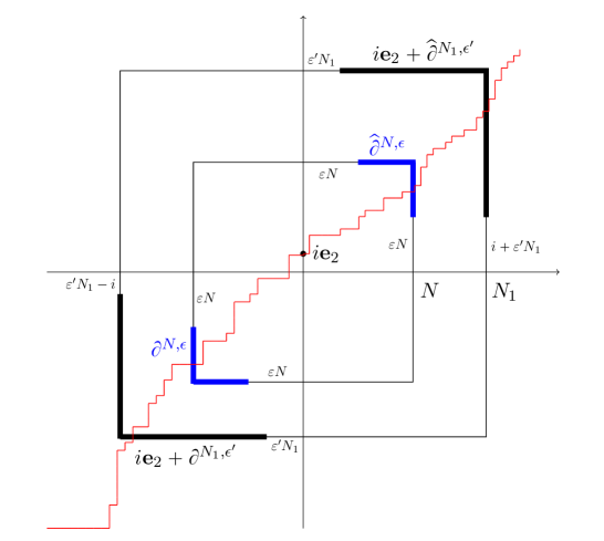
Figure 5.1. The inner $N\times N$ square is centered at $\mathbf{0}$ while the outer $N_{1}\times N_{1}$ square is centered at $i\mathbf{e}_{2}$. The (thick, dark) boundary segments of the outer square cover the (thick, light) boundary segments of the inner square. Thus the path through $i\mathbf{e}_{2}$ that crosses $\partial^{N,\varepsilon}$ and $\widehat{\partial}^{N,\varepsilon}$ is forced to also cross $i\mathbf{e}_{2}+\partial^{N_{1},\hskip 0.7pt\varepsilon^{\prime}}$ and $i\mathbf{e}_{2}+\widehat{\partial}^{N_{1},\hskip 0.7pt\varepsilon^{\prime}}$.

Let $\varepsilon=2^{-k}$ for some $k\geq 1$, $\varepsilon^{\prime}=\varepsilon/2$, and abbreviate $N_{1}=N+\lceil{N^{2/3}}\rceil$. In the scale $N_{1}$ consider the translated square $i\mathbf{e}_{2}+\llbracket-N_{1},N_{1}\rrbracket^{2}$ centered at $i\mathbf{e}_{2}$, with its boundary portions $i\mathbf{e}_{2}+\partial^{N_{1},\hskip 0.7pt\varepsilon^{\prime}}$ in the southwest and $i\mathbf{e}_{2}+\widehat{\partial}^{N_{1},\hskip 0.7pt\varepsilon^{\prime}}$ in the northeast. This translated $N_{1}$-square contains $\llbracket-N,N\rrbracket^{2}$ for all $i\in\llbracket-N^{2/3},N^{2/3}\rrbracket$.

There exists a finite constant $N_{0}(\varepsilon)$ such that $|i|+\varepsilon^{\prime}N_{1}\leq\varepsilon N$ for all $i\in\llbracket-N^{2/3},N^{2/3}\rrbracket$ and $N\geq N_{0}(\varepsilon)$. Then every path $x_{\raisebox{0.5pt}{\scaleobj{0.6}{\bullet}}}\in\mathbb{X}^{\varepsilon,\hskip 0.55ptN,\hskip 0.55pti}$ necessarily goes through both $i\mathbf{e}_{2}+\partial^{N_{1},\hskip 0.7pt\varepsilon^{\prime}}$ and $i\mathbf{e}_{2}+\widehat{\partial}^{N_{1},\hskip 0.7pt\varepsilon^{\prime}}$. In other words, $x_{\raisebox{0.5pt}{\scaleobj{0.6}{\bullet}}}$ is a member of the translate $i\mathbf{e}_{2}+\mathbb{X}^{\varepsilon^{\prime},\hskip 0.55ptN_{1},\hskip 0.55pt0}$ of the class of paths that go through the edge $e_{0}$. This is illustrated in Figure 5.1.

On the event $\mathbb{X}^{\varepsilon,\hskip 0.55ptN,\hskip 0.55pti}$ let, in the coordinatewise ordering, $X_{\partial}=\inf\{X_{\raisebox{0.5pt}{\scaleobj{0.6}{\bullet}}}\cap(i\mathbf{e}_{2}+\partial^{N_{1},\hskip 0.7pt\varepsilon^{\prime}})\}$ be the first vertex of the path $X_{\raisebox{0.5pt}{\scaleobj{0.6}{\bullet}}}$ in $i\mathbf{e}_{2}+\partial^{N_{1},\hskip 0.7pt\varepsilon^{\prime}}$ and $X_{\widehat{\partial}}=\sup\{X_{\raisebox{0.5pt}{\scaleobj{0.6}{\bullet}}}\cap(i\mathbf{e}_{2}+\widehat{\partial}^{N_{1},\hskip 0.7pt\varepsilon^{\prime}})\}$ the last vertex of the path in $i\mathbf{e}_{2}+\widehat{\partial}^{N_{1},\hskip 0.7pt\varepsilon^{\prime}}$. Note that for $u\in(i\mathbf{e}_{2}+\partial^{N_{1},\hskip 0.7pt\varepsilon^{\prime}})$ and $v\in(i\mathbf{e}_{2}+\widehat{\partial}^{N_{1},\hskip 0.7pt\varepsilon^{\prime}})$, the event $\{X_{\partial}=u,X_{\widehat{\partial}}=v\}$ depends on the entire path $X_{\raisebox{0.5pt}{\scaleobj{0.6}{\bullet}}}$ only through its edges outside $i\mathbf{e}_{2}+\llbracket-N_{1},N_{1}\rrbracket^{2}$. Suppose $\mu(\mathbb{X}^{N,\varepsilon,i})>0$ for some $\mu\in\overleftrightarrow{\text{\rm DLR}}^{\omega}$. Below we apply the Gibbs property, recall the definition (4.18) of $\mathbb{X}_{u,v}^{0}$ as the set of paths from $u$ to $v$ that take the edge $e_{0}=(\mathbf{0},\mathbf{e}_{1})$, and write $Q^{\omega}$ so that we can include explicitly translation of the weights $\omega$.

$$\mu(\mathbb{X}^{N,\varepsilon,i}) \leq\mu(i\mathbf{e}_{2}+\mathbb{X}^{\varepsilon^{\prime},\hskip 0.55ptN_{1},\hskip 0.55pt0})$$

$$\leq\sum_{u\hskip 0.9pt\in\hskip 0.9pt\partial^{N_{1}\!,\hskip 0.7pt\varepsilon^{\prime}}\!,\,v\hskip 0.9pt\in\hskip 0.9pt\widehat{\partial}^{N_{1}\!,\hskip 0.7pt\varepsilon^{\prime}}}\mu(i\mathbf{e}_{2}+\mathbb{X}_{u,v}^{0}\,|\,X_{\partial}=i\mathbf{e}_{2}+u,X_{\widehat{\partial}}=i\mathbf{e}_{2}+v)\hskip 0.9pt\mu(X_{\partial}=i\mathbf{e}_{2}+u,X_{\widehat{\partial}}=i\mathbf{e}_{2}+v)$$

$$=\sum_{u\hskip 0.9pt\in\hskip 0.9pt\partial^{N_{1}\!,\hskip 0.7pt\varepsilon^{\prime}}\!,\,v\hskip 0.9pt\in\hskip 0.9pt\widehat{\partial}^{N_{1}\!,\hskip 0.7pt\varepsilon^{\prime}}}Q^{\omega}_{i\mathbf{e}_{2}+u,\hskip 0.55pti\mathbf{e}_{2}+v}(i\mathbf{e}_{2}+\mathbb{X}_{u,v}^{0})\hskip 0.9pt\mu(X_{\partial}=i\mathbf{e}_{2}+u,X_{\widehat{\partial}}=i\mathbf{e}_{2}+v)$$

$$\leq\max_{u\hskip 0.9pt\in\hskip 0.9pt\partial^{N_{1}\!,\hskip 0.7pt\varepsilon^{\prime}}\!,\,v\hskip 0.9pt\in\hskip 0.9pt\widehat{\partial}^{N_{1}\!,\hskip 0.7pt\varepsilon^{\prime}}}Q^{\omega}_{i\mathbf{e}_{2}+u,\hskip 0.55pti\mathbf{e}_{2}+v}(i\mathbf{e}_{2}+\mathbb{X}_{u,v}^{0})=\max_{u\hskip 0.9pt\in\hskip 0.9pt\partial^{N_{1}\!,\hskip 0.7pt\varepsilon^{\prime}}\!,\,v\hskip 0.9pt\in\hskip 0.9pt\widehat{\partial}^{N_{1}\!,\hskip 0.7pt\varepsilon^{\prime}}}Q^{T_{i\mathbf{e}_{2}}\omega}_{u,\hskip 0.55ptv}(\mathbb{X}_{u,v}^{0})$$

$$=\max_{u\hskip 0.9pt\in\hskip 0.9pt\partial^{N_{1}\!,\hskip 0.7pt\varepsilon^{\prime}}\!,\,v\hskip 0.9pt\in\hskip 0.9pt\widehat{\partial}^{N_{1}\!,\hskip 0.7pt\varepsilon^{\prime}}}p^{u,v}_{0}(T_{i\mathbf{e}_{2}}\omega)=\xi^{\varepsilon^{\prime}}_{N_{1}}(T_{i\mathbf{e}_{2}}\omega).$$

Then (5.3) gives, on the event $\Omega^{\prime}$,

$$\mu(\mathbb{X}^{\varepsilon,i})\leq\varliminf_{N\to\infty}\mu(\mathbb{X}^{N,\varepsilon,i})\leq\varliminf_{N\to\infty}\xi^{\varepsilon^{\prime}}_{N_{1}}\circ T_{i\mathbf{e}_{2}}=0.$$

(5.2) has been verified. This completes the proof of the main result Theorem 2.7. ∎

Appendix A General properties of planar directed polymers

This appendix covers some consequences of the general polymer formalism. Begin again with the partition function with given weights $Y_{x}>0$:

(A.1) $$Z_{u,v}=\sum_{x_{\raisebox{-0.5pt}{\scaleobj{0.5}{\bullet}}}\hskip 0.7pt\in\hskip 0.7pt\mathbb{X}_{u,v}}\prod_{i=0}^{|v-u|_{1}}Y_{x_{i}}\quad\text{for $u\leq v$ on $\mathbb{Z}^{2}$,}$$

with $Z_{u,v}=0$ if $u\leq v$ fails.

A.1. Ratio weights and nested polymers

Keeping the base point $u$ fixed, define ratio weights for varying $x$:

$$I_{x}=I_{u,x}=\frac{Z_{u,x}}{Z_{u,x-\mathbf{e}_{1}}}\quad\text{ and }\quad J_{x}=J_{u,x}=\frac{Z_{u,x}}{Z_{u,x-\mathbf{e}_{2}}}.$$

The ratio weights can be calculated inductively from boundary values $I_{u+k\mathbf{e}_{1}}=Y_{u+k\mathbf{e}_{1}}$ and $J_{u+\ell\mathbf{e}_{2}}=Y_{u+\ell\mathbf{e}_{2}}$ for $k,\ell\geq 1$, by iterating

(A.2) $$I_{x}=Y_{x}\bigl{(}1+I_{x-\mathbf{e}_{2}}J_{x-\mathbf{e}_{1}}^{-1}\bigr{)}\quad\text{ and }\quad J_{x}=Y_{x}\bigl{(}J_{x-\mathbf{e}_{1}}I_{x-\mathbf{e}_{2}}^{-1}+1\bigr{)}.$$

Let $u\leq v$ on $\mathbb{Z}^{2}$. On the boundary of the quadrant $v+\mathbb{Z}_{\geq 0}^{2}$, put ratio weights of the partition functions with base point $u$:

$$Y^{(u)}_{v+i\mathbf{e}_{r}}=\frac{Z_{u,v+i\mathbf{e}_{r}}}{Z_{u,v+(i-1)\mathbf{e}_{r}}}\qquad\text{for }\ r\in\{1,2\}\ \text{ and }\ i\geq 1.$$

The ratio weights dominate the original weights: $Y^{(u)}_{v+i\mathbf{e}_{r}}\geq Y_{v+i\mathbf{e}_{r}}$, and equality holds iff $v=u+m\mathbf{e}_{r}$ for some $m\geq 0$.

Define a partition function $Z^{(u)}_{v,w}$ that uses these boundary weights and ignores the first weight of the path: for $k,\ell\geq 1$ and $w\in v+\mathbb{Z}_{>0}^{2}$,

$$Z^{(u)}_{v,v} =1,\quad Z^{(u)}_{v,v+k\mathbf{e}_{1}}=\prod_{i=1}^{k}Y^{(u)}_{v+i\mathbf{e}_{1}},\quad Z^{(u)}_{v,v+\ell\mathbf{e}_{2}}=\prod_{j=1}^{\ell}Y^{(u)}_{v+j\mathbf{e}_{2}}$$

$$Z^{(u)}_{v,w} =\sum_{k=1}^{w_{1}-v_{1}}\biggl{(}\;\prod_{i=1}^{k}Y^{(u)}_{v+i\mathbf{e}_{1}}\biggr{)}Z_{v+k\mathbf{e}_{1}+\mathbf{e}_{2},w}+\sum_{\ell=1}^{w_{2}-v_{2}}\biggl{(}\;\prod_{j=1}^{\ell}Y^{(u)}_{v+j\mathbf{e}_{2}}\biggr{)}Z_{v+\mathbf{e}_{1}+\ell\mathbf{e}_{2},w}.$$

For $w\in v+\mathbb{Z}_{>0}^{2}$ the definition from above can be rewritten as follows:

$$Z^{(u)}_{v,w} =\frac{1}{Z_{u,v}}\sum_{k=1}^{w_{1}-v_{1}}Z_{u,v+k\mathbf{e}_{1}}Z_{v+k\mathbf{e}_{1}+\mathbf{e}_{2},w}+\frac{1}{Z_{u,v}}\sum_{\ell=1}^{w_{2}-v_{2}}Z_{u,v+\ell\mathbf{e}_{2}}Z_{v+\mathbf{e}_{1}+\ell\mathbf{e}_{2},w}.$$

and thus for all $u\leq v\leq w$ we have the identity

(A.3) $$Z^{(u)}_{v,w}=\frac{Z_{u,w}}{Z_{u,v}}.$$

Ratio variables satisfy

(A.4) $$I_{u,x}=\frac{Z_{u,x}}{Z_{u,x-\mathbf{e}_{1}}}=\frac{Z_{u,v}\,Z^{(u)}_{v,x}}{Z_{u,v}\,Z^{(u)}_{v,x-\mathbf{e}_{1}}}=\frac{Z^{(u)}_{v,x}}{Z^{(u)}_{v,x-\mathbf{e}_{1}}}=I^{(u)}_{v,x}$$

with the analogous identity $J_{u,x}=J^{(u)}_{v,x}$.

Recall the definition (3.5) of ${\tau}_{u,v,w}$. Let $Q^{(u)}_{v,w}$ be the quenched path probability on $\mathbb{X}_{v,w}$ that corresponds to the partition function $Z^{(u)}_{v,w}$. Then we have the identity

(A.5) $$Q_{u,w}({\tau}_{u,v,w}=\ell)=Q^{(u)}_{v,w}({\tau}_{v,w}=\ell)\qquad\text{for }\ 0\neq\ell\in\mathbb{Z}.$$

Here is the derivation for the case where the path from $u$ to $w$ goes above $v$. Let $k\geq 1$. Apply (A.3) and (A.4).

$$Q_{u,w}({\tau}_{u,v,w}=-k) =\frac{Z_{u,v+k\mathbf{e}_{2}}Z_{v+\mathbf{e}_{1}+k\mathbf{e}_{2},w}}{Z_{u,w}}=\frac{Z_{u,v}\bigl{(}\,\prod_{j=1}^{k}J_{u,v+j\mathbf{e}_{2}}\bigr{)}Z_{v+\mathbf{e}_{1}+k\mathbf{e}_{2},w}}{Z_{u,w}}$$

$$=\frac{\bigl{(}\,\prod_{j=1}^{k}J^{(u)}_{v,v+j\mathbf{e}_{2}}\bigr{)}Z_{v+\mathbf{e}_{1}+k\mathbf{e}_{2},w}}{Z^{(u)}_{v,w}}=Q^{(u)}_{v,w}({\tau}_{v,w}=-k).$$

A.2. Inequalities for point-to-point partition functions

We state several inequalities that follow from the next basic lemma. The inequalities in (A.6) below are proved together by induction on $x$ and $y$, beginning with $x=u+k\mathbf{e}_{1}$ and $y=u+\ell\mathbf{e}_{2}$. The induction step is carried out by formulas (A.2).

Lemma A.1.

Fix a base point $u$. Let $\{Y^{(1)}_{x}\}$ and $\{Y^{(2)}_{x}\}$ be strictly positive weights from which partition functions $Z^{(1)}_{u,v}$ and $Z^{(2)}_{u,v}$ are defined. Assume that $Y^{(1)}_{u}=Y^{(2)}_{u}$, $Y^{(1)}_{u+k\mathbf{e}_{1}}\leq Y^{(2)}_{u+k\mathbf{e}_{1}}$, $Y^{(2)}_{u+\ell\mathbf{e}_{2}}\leq Y^{(1)}_{u+\ell\mathbf{e}_{2}}$ and $Y^{(1)}_{x}=Y^{(2)}_{x}$ for all $k,\ell\geq 1$ and $x\in u+\mathbb{Z}_{>0}^{2}$. Then we have the following inequalities for $x\geq u+\mathbf{e}_{1}$ and $y\geq u+\mathbf{e}_{2}$:

(A.6) $$\frac{Z^{(1)}_{u,x}}{Z^{(1)}_{u,x-\mathbf{e}_{1}}}\leq\frac{Z^{(2)}_{u,x}}{Z^{(2)}_{u,x-\mathbf{e}_{1}}}\qquad\text{and}\qquad\frac{Z^{(2)}_{u,y}}{Z^{(2)}_{u,y-\mathbf{e}_{2}}}\leq\frac{Z^{(1)}_{u,y}}{Z^{(1)}_{u,y-\mathbf{e}_{2}}}.$$

From the lemma we obtain the following pair of inequalities:

(A.7) $$\frac{Z_{u,z}}{Z_{u,z-\mathbf{e}_{1}}}\leq\frac{Z_{u+\mathbf{e}_{1},z}}{Z_{u+\mathbf{e}_{1},z-\mathbf{e}_{1}}}\qquad\text{and}\qquad\frac{Z_{u,z}}{Z_{u,z-\mathbf{e}_{1}}}\leq\frac{Z_{u-\mathbf{e}_{2},z}}{Z_{u-\mathbf{e}_{2},z-\mathbf{e}_{1}}}.$$

The first inequality above follows from the first inequality of (A.6) by letting the weights $\{Y_{u+j\mathbf{e}_{2}}\}_{j\geq 1}$ tend to zero, and the second one by letting the weights $\{Y_{u-\mathbf{e}_{2}+i\mathbf{e}_{1}}\}_{i\geq 1}$ tend to zero.

Lemma A.2.

Let $x,y,z\in\mathbb{Z}^{2}$ be such that $x\preccurlyeq y$ and $x,y\leq z-\mathbf{e}_{1}-\mathbf{e}_{2}$. We then have

(A.8) $$\frac{Z_{x,z}}{Z_{x,z-\mathbf{e}_{1}}}\leq\frac{Z_{y,z}}{Z_{y,z-\mathbf{e}_{1}}}$$

(A.9) $$\frac{Z_{y,z}}{Z_{y,z-\mathbf{e}_{2}}}\leq\frac{Z_{x,z}}{Z_{x,z-\mathbf{e}_{2}}}.$$

Proof.

(A.8) follows from repeated application of (A.7) along the steps $\mathbf{e}_{1}$ and $-\mathbf{e}_{2}$ from $x$ to $y$. Transposing (A.8) gives (A.9). ∎

Since $u+k\mathbf{e}_{1}\succcurlyeq u$ and $u+\ell\mathbf{e}_{2}\preccurlyeq u$ for $k,\ell\geq 0$, inequalities (A.8)–(A.9) imply also these for $1\leq k<(x-u)\cdot\mathbf{e}_{1}$ and $1\leq\ell<(y-u)\cdot\mathbf{e}_{2}$:

(A.10) $$\frac{Z_{u,x}}{Z_{u,x-\mathbf{e}_{1}}}\leq\frac{Z_{u,x}({\tau}_{u,x}\geq k)}{Z_{u,x-\mathbf{e}_{1}}({\tau}_{u,x-\mathbf{e}_{1}}\geq k)}\quad\text{ and }\quad\frac{Z_{u,y}}{Z_{u,y-\mathbf{e}_{2}}}\leq\frac{Z_{u,y}({\tau}_{u,y}\leq-\ell)}{Z_{u,y-\mathbf{e}_{2}}({\tau}_{u,y-\mathbf{e}_{2}}\leq-\ell)}.$$

To illustrate the explicit proof of the first one:

$$\frac{Z_{u,x}({\tau}_{u,x}\geq k)}{Z_{u,x-\mathbf{e}_{1}}({\tau}_{u,x-\mathbf{e}_{1}}\geq k)}=\frac{(\,\prod_{i=0}^{k-1}Y_{u+i\mathbf{e}_{1}})\,Z_{u+k\mathbf{e}_{1},x}}{(\,\prod_{i=0}^{k-1}Y_{u+i\mathbf{e}_{1}})\,Z_{u+k\mathbf{e}_{1},x-\mathbf{e}_{1}}}=\frac{Z_{u+k\mathbf{e}_{1},x}}{Z_{u+k\mathbf{e}_{1},x-\mathbf{e}_{1}}}\geq\frac{Z_{u,x}}{Z_{u,x-\mathbf{e}_{1}}}.$$

A.3. Ordering of path measures

The down-right partial order $\preccurlyeq$ on $\mathbb{R}^{2}$ and $\mathbb{Z}^{2}$ was defined by $(x_{1},x_{2})\preccurlyeq(y_{1},y_{2})$ if $x_{1}\leq y_{1}$ and $x_{2}\geq y_{2}$. Extend this relation to pairs of vertices $(x^{1},y^{1}),(x^{2},y^{2})\in\mathbb{Z}^{2}\times\mathbb{Z}^{2}$ as follows (illustrated in Figure A.1):

(A.11) $$(x^{1},y^{1})\preccurlyeq(x^{2},y^{2})\quad\text{ if }x^{1}\leq y^{1},\ x^{2}\leq y^{2},\ x^{1}\preccurlyeq x^{2}\text{ and }y^{1}\preccurlyeq y^{2}.$$

Extend this relation further to finite paths: $\pi^{1}\in\mathbb{X}_{x^{1},y^{1}}$ and $\pi^{2}\in\mathbb{X}_{x^{2},y^{2}}$ satisfy $\pi^{1}\preccurlyeq\pi^{2}$ if the pairs of endpoints satisfy $(x^{1},y^{1})\preccurlyeq(x^{2},y^{2})$ and whenever $z^{1}\in\pi^{1}$, $z^{2}\in\pi^{2}$, and $z^{1}\cdot(\mathbf{e}_{1}+\mathbf{e}_{2})=z^{2}\cdot(\mathbf{e}_{1}+\mathbf{e}_{2})$, we have $z^{1}\preccurlyeq z^{2}$. Pictorially, in a very clear sense, $\pi^{1}$ lies (weakly) above and to the left of $\pi^{2}$. See again Figure A.1.

Figure A.1. On the left the pairs $(x^{1},y^{1})$ and $(x^{2},y^{2})$ satisfy $(x^{1},y^{1})\preccurlyeq(x^{2},y^{2})$, while on the right this relation fails. Consistently with this, on the left the paths $\pi^{1}\in\mathbb{X}_{x^{1},y^{1}}$ and $\pi^{2}\in\mathbb{X}_{x^{2},y^{2}}$ satisfy $\pi^{1}\preccurlyeq\pi^{2}$ but on the right this fails.

Let $\mu$ and $\nu$ be probability measures on the finite path spaces $\mathbb{X}_{x^{1},y^{1}}$ and $\mathbb{X}_{x^{2},y^{2}}$, respectively. We write $\mu\preccurlyeq\nu$ if there exist random paths $X^{1}\in\mathbb{X}_{x^{1},y^{1}}$ and $X^{2}\in\mathbb{X}_{x^{2},y^{2}}$ on a common probability space such that $X^{1}\sim\mu$, $X^{2}\sim\nu$, and $X^{1}\preccurlyeq X^{2}$. In other words, $\mu\preccurlyeq\nu$ if $\nu$ stochastically dominates $\mu$ under the partial order $\preccurlyeq$ on paths. The following shows that for fixed weights there exists a coupling of all the quenched polymer distributions $\{Q_{x,y}\}_{x\leq y}$ on the lattice $\mathbb{Z}^{2}$ so that $Q_{x,y}\preccurlyeq Q_{u,v}$ whenever $(x,y)\preccurlyeq(u,v)$.

Lemma A.3.

Let $(Y_{x})_{x\hskip 0.7pt\in\hskip 0.7pt\mathbb{Z}^{2}}$ be an assignment of strictly positive weights on the lattice $\mathbb{Z}^{2}$. Then there exists a coupling of up-right random paths $\{\pi^{x,y}\}_{x\leq y}$ such that $\pi^{x,y}\in\mathbb{X}_{x,y}$, $\pi^{x,y}$ has the quenched polymer distribution $Q_{x,y}$, and $\pi^{x,y}\preccurlyeq\pi^{u,v}$ whenever $(x,y)\preccurlyeq(u,v)$.

Proof.

Let $\{U_{z}\}_{z\in\mathbb{Z}^{2}}$ be an assignment of i.i.d. uniform random variables $U_{z}\sim\text{\rm Unif}(0,1)$ to the vertices of $\mathbb{Z}^{2}$, defined under some probability measure $\mathbf{P}$. For each pair $x\leq z$ such that $x\neq z$, define the down-left pointing random unit vector

(A.12) $$V^{x}(z)=\begin{cases}-\mathbf{e}_{1},&\text{if }\ \ \dfrac{Y_{z}Z_{x,z-\mathbf{e}_{1}}}{Z_{x,z}}\geq U_{z}\\[5.0pt] -\mathbf{e}_{2},&\text{if }\ \ \dfrac{Y_{z}Z_{x,z-\mathbf{e}_{2}}}{Z_{x,z}}>1-U_{z}.\end{cases}$$

If $z=x+k\mathbf{e}_{i}$ this gives $V^{x}(z)=-\mathbf{e}_{i}$ due to the convention $Z_{u,v}=0$ when $u\leq v$ fails. Hence any path that starts at some vertex $y\geq x$ distinct from $x$ and follows the steps from each $z$ to $z+V^{x}(z)$ terminates at $x$.

Since the paths from distinct points that follow increments $V^{x}(z)$ for a given $x$ eventually coalesce, a realization of $\{V^{x}(z)\}_{z\geq x:\,z\neq x}$ defines a spanning tree $\mathcal{T}^{x}$ rooted at $x$ on the nearest-neighbor graph on the quadrant $x+\mathbb{Z}_{\geq 0}^{2}$. For $x\leq y$ let $\pi^{x,y}\in\mathbb{X}_{x,y}$ be the path that connects $x$ and $y$ in the tree $\mathcal{T}^{x}$. Then for any path $x_{\raisebox{0.5pt}{\scaleobj{0.6}{\bullet}}}\in\mathbb{X}_{x,y}$, (A.12) implies that $Q_{x,y}(x_{\raisebox{0.5pt}{\scaleobj{0.6}{\bullet}}})=\mathbf{P}(\pi^{x,y}=x_{\raisebox{0.5pt}{\scaleobj{0.6}{\bullet}}}).$ In other words, through the random paths $\{\pi^{x,y}\}_{x\leq y}$ we have a coupling of the quenched polymer distributions $\{Q_{x,y}\}_{x\leq y}$.

Let $x\preccurlyeq u$. By Lemma A.2

$$\frac{Y_{z}Z_{x,z-\mathbf{e}_{1}}}{Z_{x,z}}\geq\frac{Y_{z}Z_{u,z-\mathbf{e}_{1}}}{Z_{u,z}}\quad\text{ and }\quad\frac{Y_{z}Z_{u,z-\mathbf{e}_{1}}}{Z_{u,z}}\geq\frac{Y_{z}Z_{x,z-\mathbf{e}_{2}}}{Z_{x,z}}.$$

Hence

(A.13) $$\{V^{x}(z)=-\mathbf{e}_{2}\} \subseteq\{V^{u}(z)=-\mathbf{e}_{2}\}$$

$$\text{and}\qquad\{V^{u}(z)=-\mathbf{e}_{1}\} \subseteq\{V^{x}(z)=-\mathbf{e}_{1}\}.$$

It follows from (A.13) that two paths satisfy $\pi^{x,y}\preccurlyeq\pi^{u,v}$ whenever $(x,y)\preccurlyeq(u,v)$. This is because if these paths share a vertex $z$, then their subsequent down-left steps satisfy $z+V^{x}(z)\preccurlyeq z+V^{u}(z)$. ∎

Let $o\leq x$. In the tree $\mathcal{T}^{o}$ constructed above, the path from $x$ down to $o$ stays weakly to the left of the path from $x+\mathbf{e}_{1}$ down to $o$. This gives the inequality below:

(A.14) $$\text{for vertices }o\leq x\text{ and }k\geq 1,\quad Q_{o,x}(t_{\mathbf{e}_{1}}\geq k)\leq Q_{o,x+\mathbf{e}_{1}}(t_{\mathbf{e}_{1}}\geq k).$$

A.4. Polymers on the upper half-plane

The stationary inverse-gamma polymer process that is our tool for calculations will be constructed on a half-plane. This section defines the notational apparatus for this purpose, borrowed from the forthcoming work [31].

Define mappings of bi-infinite sequences: $I=(I_{k})_{k\hskip 0.55pt\in\hskip 0.55pt\mathbb{Z}}$ and $Y=(Y_{j})_{j\in\mathbb{Z}}$ in $\mathbb{R}_{>0}^{\mathbb{Z}}$ that are assumed to satisfy

(A.15) $$C(I,Y)=\lim_{m\to\,-\infty}\sum_{j=m}^{0}{Y_{j}}\prod_{i=j+1}^{0}\frac{Y_{i}}{I_{i}}<\infty.$$

From these inputs, three outputs $\widetilde{I}=(\widetilde{I}_{k})_{k\hskip 0.55pt\in\hskip 0.55pt\mathbb{Z}}$, $J=(J_{k})_{k\hskip 0.55pt\in\hskip 0.55pt\mathbb{Z}}$ and $\widetilde{Y}=(\widetilde{Y}_{k})_{k\hskip 0.55pt\in\hskip 0.55pt\mathbb{Z}}$, also elements of $\mathbb{R}_{>0}^{\mathbb{Z}}$, are constructed as follows.

Let $Z=(Z_{k})_{k\hskip 0.55pt\in\hskip 0.55pt\mathbb{Z}}$ be any function on $\mathbb{Z}$ that satisfies $I_{k}=Z_{k}/Z_{k-1}$. This defines $Z$ up to a positive multiplicative constant. Define the sequence $\widetilde{Z}=(\widetilde{Z}_{\ell})_{\ell\in\mathbb{Z}}$ by

(A.16) $$\widetilde{Z}_{\ell}=\sum_{k:\,k\leq\ell}Z_{k}\,\prod_{i=k}^{\ell}Y_{i}\,,\quad\ell\in\mathbb{Z}.$$

Under assumption (A.15) the sum on the right-hand side of (A.16) is finite. To check this choose a particular $Z$ by setting $Z_{0}=1$. (Any other admissible $Z$ is a constant multiple of this one.) Then $Z_{k}=\prod_{i=k+1}^{0}I_{i}^{-1}$ for $k\leq-1$.

$$\widetilde{Z}_{\ell} =\sum_{k:\,k\leq\ell\wedge 0}Z_{k}\,\prod_{i=k}^{\ell}Y_{i}+\sum_{k:\,1\leq k\leq\ell}Z_{k}\,\prod_{i=k}^{\ell}Y_{i}$$

$$=\sum_{k:\,k\leq\ell\wedge 0}\biggl{(}\;\prod_{i=k+1}^{0}I_{i}^{-1}\biggr{)}\biggl{(}\;\prod_{i=k}^{0}Y_{i}\biggr{)}C_{\ell}(Y)+\sum_{k:\,1\leq k\leq\ell}Z_{k}\,\prod_{i=k}^{\ell}Y_{i}$$

$$\leq C(I,Y)C_{\ell}(Y)+\sum_{k:\,1\leq k\leq\ell}Z_{k}\,\prod_{i=k}^{\ell}Y_{i}<\infty\,.$$

For $k\in\mathbb{Z}$ define

(A.17) $$\widetilde{I}_{k}=\widetilde{Z}_{k}/\widetilde{Z}_{k-1},$$

(A.18) $$J_{k}=\widetilde{Z}_{k}/Z_{k},$$

(A.19) $$\widetilde{Y}_{k}=(I_{k}^{-1}+J_{k-1}^{-1})^{-1}.$$

The sequences $\widetilde{I}$, $J$ and $\widetilde{Y}$ are well-defined positive real sequences, and they do not depend on the choice of the function $Z$ as long as $Z$ has ratios $I_{k}=Z_{k}/Z_{k-1}$. The three mappings are denoted by

(A.20) $$\widetilde{I}=D(I,Y),\quad J=S(I,Y),\quad\text{and}\quad\widetilde{Y}=R(I,Y).$$

Beginning from $\widetilde{Z}_{k}=Y_{k}(Z_{k}+\widetilde{Z}_{k-1})$ we derive these equations:

(A.21) $$\widetilde{I}_{k} =Y_{k}\biggl{(}\frac{I_{k}}{J_{k-1}}+1\biggr{)}=\frac{Y_{k}}{\widetilde{Y}_{k}}I_{k}$$

(A.22) $$\text{and }\qquad J_{k} =Y_{k}\biggl{(}1+\frac{J_{k-1}}{I_{k}}\biggr{)}=\frac{Y_{k}}{\widetilde{Y}_{k}}J_{k-1}.$$

The last formula iterates as follows: for $\ell<m$,

(A.23) $$J_{m}=J_{\ell}\prod_{i=\ell+1}^{m}\frac{Y_{i}}{I_{i}}+\sum_{j=\ell+1}^{m}Y_{j}\prod_{i=j+1}^{m}\frac{Y_{i}}{I_{i}}.$$

We record two inequalities. From (A.21),

(A.24) $$\widetilde{I}_{j}\geq Y_{j}.$$

If we start with two coordinatewise ordered boundary weights $I_{j}\leq I^{\prime}_{j}$ (for all $j$) and use the same bulk weights $Y$ to compute vertical ratio weights $J=S(I,Y)$ and $J^{\prime}=S(I^{\prime},Y)$, the inequality is reversed:

(A.25) $$J^{\prime}_{k}=\frac{\widetilde{Z}^{\prime}_{k}}{Z^{\prime}_{k}}=\sum_{j:\,j\leq k}Y_{j}\,\prod_{i=j+1}^{k}\frac{Y_{i}}{I^{\prime}_{i}}\leq\sum_{j:\,j\leq k}Y_{j}\,\prod_{i=j+1}^{k}\frac{Y_{i}}{I_{i}}=J_{k}.$$

Further manipulation gives the next lemma. We omit the proof.

Lemma A.4.

To calculate $\{\widetilde{I}_{k},J_{k},\widetilde{Y}_{k}:k\leq m\}$, we need only the input $\{I_{k},Y_{k}:k\leq m\}$.

The next lemma is nontrivial and we include a complete proof.

Lemma A.5.

The identity $D\bigl{(}D(A,I),Y\bigr{)}=D\bigl{(}D(A,R(I,Y)),D(I,Y)\bigr{)}$ holds whenever the sequences $I,A,Y$ are such that the operations are well-defined.

Proof.

Choose $(Z_{j})$ and $(B_{j})$ so that $Z_{j}/Z_{j-1}=I_{j}$ and $B_{j}/B_{j-1}=A_{j}$. Then the output of $D(A,I)$ is the ratio sequence $(\widetilde{B}_{\ell}/\widetilde{B}_{\ell-1})_{\ell}$ of

$$\widetilde{B}_{\ell}=\sum_{k:\,k\leq\ell}B_{k}\prod_{i=k}^{\ell}I_{i}.$$

Next, the output of $D(D(A,I),Y)$ is the ratio sequence $(H_{m}/H_{m-1})_{m}$ of

$$H_{m}=\sum_{\ell:\,\ell\leq m}\widetilde{B}_{\ell}\prod_{j=\ell}^{m}Y_{j}=\sum_{k:\,k\leq m}B_{k}\sum_{\ell=k}^{m}\Bigl{(}\;\prod_{i=k}^{\ell}I_{i}\Bigr{)}\Bigl{(}\;\prod_{j=\ell}^{m}Y_{j}\Bigr{)}.$$

Similarly, define first

$$\widetilde{Z}_{j}=\sum_{k:\,k\leq j}Z_{k}\prod_{i=k}^{j}Y_{i}\quad\text{and}\quad\widetilde{I}_{j}=\frac{\widetilde{Z}_{j}}{\widetilde{Z}_{j-1}}$$

so that $\widetilde{I}=D(I,Y)$. Let $\widetilde{Y}=R(I,Y)$ and then

$$\widecheck{B}_{\ell}=\sum_{k:\,k\leq\ell}B_{k}\prod_{i=k}^{\ell}\widetilde{Y}_{i}.$$

Then the output of $D\bigl{(}D(A,R(I,Y)),D(I,Y)\bigr{)}=D(D(A,\widetilde{Y}),\widetilde{I}\,)$ is the ratio sequence of

$$\widetilde{H}_{m}=\sum_{\ell:\,\ell\leq m}\widecheck{B}_{\ell}\prod_{j=\ell}^{m}\widetilde{I}_{j}=\sum_{k:\,k\leq m}B_{k}\sum_{\ell=k}^{m}\Bigl{(}\;\prod_{i=k}^{\ell}\widetilde{Y}_{i}\Bigr{)}\Bigl{(}\;\prod_{j=\ell}^{m}\widetilde{I}_{j}\Bigr{)}.$$

The lemma follows from $H=\widetilde{H}$, which we verify by checking that for all $k\leq m$,

(A.26) $$\sum_{\ell=k}^{m}\Bigl{(}\;\prod_{i=k}^{\ell}I_{i}\Bigr{)}\Bigl{(}\;\prod_{j=\ell}^{m}Y_{j}\Bigr{)}=\sum_{\ell=k}^{m}\Bigl{(}\;\prod_{i=k}^{\ell}\widetilde{Y}_{i}\Bigr{)}\Bigl{(}\;\prod_{j=\ell}^{m}\widetilde{I}_{j}\Bigr{)}.$$

We fix $k$ and prove this by induction on $m$. The case $m=k$ follows from (A.19) and (A.21):

$$\widetilde{Y}_{k}\widetilde{I}_{k}=\frac{Y_{k}\bigl{(}\frac{I_{k}}{J_{k-1}}+1\bigr{)}}{\frac{1}{I_{k}}+\frac{1}{J_{k-1}}}=I_{k}Y_{k}.$$

To prove the induction step, we introduce two auxiliary quantities by adding terms separately on the left and right of (A.26): let

$$T_{m}=J_{k-1}\prod_{j=k}^{m}Y_{j}+\sum_{\ell=k}^{m}\Bigl{(}\;\prod_{i=k}^{\ell}I_{i}\Bigr{)}\Bigl{(}\;\prod_{j=\ell}^{m}Y_{j}\Bigr{)}$$

and

$$\widetilde{T}_{m}=\sum_{\ell=k}^{m}\Bigl{(}\;\prod_{i=k}^{\ell}\widetilde{Y}_{i}\Bigr{)}\Bigl{(}\;\prod_{j=\ell}^{m}\widetilde{I}_{j}\Bigr{)}+\Bigl{(}\;\prod_{i=k}^{m}\widetilde{Y}_{i}\Bigr{)}J_{m}.$$

Repeated application of (A.22) implies that $J_{k-1}\prod_{j=k}^{m}Y_{j}=(\;\prod_{i=k}^{m}\widetilde{Y}_{i})J_{m}$. Thus (A.26) is equivalent to $\widetilde{T}_{m}=T_{m}$.

First observe that $T_{m+1}=T_{m}\widetilde{I}_{m+1}$ for $m\geq k$. This follows from checking inductively the pair of identities

$$\frac{T_{m}}{\prod_{i=k}^{m}I_{i}}=J_{m}\quad\text{and}\quad\frac{T_{m+1}}{T_{m}}=\widetilde{I}_{m+1}\quad\text{for }\ m\geq k.$$

This relies on the first equalities of the iterative formulas (A.21) and (A.22).

Now assume that $\widetilde{T}_{m}=T_{m}$. We show that $\widetilde{T}_{m+1}=\widetilde{T}_{m}\widetilde{I}_{m+1}$ which then implies $\widetilde{T}_{m+1}=T_{m+1}$.

$$\widetilde{T}_{m+1} =\sum_{\ell=k}^{m}\Bigl{(}\;\prod_{i=k}^{\ell}\widetilde{Y}_{i}\Bigr{)}\Bigl{(}\;\prod_{j=\ell}^{m}\widetilde{I}_{j}\Bigr{)}\widetilde{I}_{m+1}+\Bigl{(}\;\prod_{i=k}^{m}\widetilde{Y}_{i}\Bigr{)}\widetilde{Y}_{m+1}\widetilde{I}_{m+1}+\Bigl{(}\;\prod_{i=k}^{m}\widetilde{Y}_{i}\Bigr{)}\widetilde{Y}_{m+1}J_{m+1}$$

$$=\widetilde{T}_{m}\widetilde{I}_{m+1}+\Bigl{(}\;\prod_{i=k}^{m}\widetilde{Y}_{i}\Bigr{)}\bigl{(}-J_{m}\widetilde{I}_{m+1}+\widetilde{Y}_{m+1}\widetilde{I}_{m+1}+\widetilde{Y}_{m+1}J_{m+1}\bigr{)}.$$

The last expression in parentheses vanishes because $J_{m}\widetilde{I}_{m+1}=Y_{m+1}(I_{m+1}+J_{m})$, $\widetilde{Y}_{m+1}\widetilde{I}_{m+1}=Y_{m+1}I_{m+1}$ and $\widetilde{Y}_{m+1}J_{m+1}=Y_{m+1}J_{m}$. ∎

Appendix B The inverse-gamma polymer

This section reviews the ratio-stationary inverse-gamma polymer introduced in [30] and then constructs the two-variable jointly ratio-stationary process, which is a special case of the multivariate construction from the forthcoming work [31].

B.1. Inverse-gamma weights

Recall the inverse gamma distribution from (2.13) and the mean from (3.6).

Lemma B.1.

Define the mapping $(I,J,Y)\mapsto(I^{\prime},J^{\prime},Y^{\prime})$ on $\mathbb{R}_{>0}^{3}$ by

(B.1) $$I^{\prime}=Y\biggl{(}1+\frac{I}{J}\biggr{)}\,,\quad J^{\prime}=Y\biggl{(}1+\frac{J}{I}\biggr{)}\,,\quad Y^{\prime}=\frac{1}{I^{-1}+J^{-1}}.$$

1. $(I,J,Y)\mapsto(I^{\prime},J^{\prime},Y^{\prime})$ is an involution.

2. Let $\alpha,\beta>0$. Suppose that $I,J,Y$ are independent random variables with distributions $I\sim{\rm Ga}^{-1}(\alpha)$, $J\sim{\rm Ga}^{-1}(\beta)$ and $Y\sim{\rm Ga}^{-1}(\alpha+\beta)$. Then the triple $(I^{\prime},J^{\prime},Y^{\prime})$ has the same distribution as $(I,J,Y)$.

Proof.

Part (b) follows by applying the beta-gamma algebra to the reciprocals that satisfy

$$\frac{1}{I^{\prime}}=Y^{-1}\frac{I^{-1}}{I^{-1}+J^{-1}}\,,\quad\frac{1}{J^{\prime}}=Y^{-1}\frac{J^{-1}}{I^{-1}+J^{-1}}\quad\text{and}\quad\frac{1}{Y^{\prime}}=I^{-1}+J^{-1}.\qed$$

Lemma B.2.

Let $0<\rho<\sigma$. Let $I=(I_{k})_{k\hskip 0.55pt\in\hskip 0.55pt\mathbb{Z}}$ and $Y=(Y_{j})_{j\in\mathbb{Z}}$ be mutually independent random variables such that $I_{k}\sim{\rm Ga}^{-1}(\rho)$ and $Y_{j}\sim{\rm Ga}^{-1}(\sigma)$. Use mappings (A.20) to define

$$\widetilde{I}=D(I,Y)\,\quad\widetilde{Y}=R(I,Y)\quad\text{and}\quad J=S(I,Y).$$

Let $V_{k}=(\{\widetilde{I}_{j}\}_{j\leq k},\,J_{k},\,\{\widetilde{Y}_{j}\}_{j\leq k})$.

1. $\{V_{k}\}_{k\hskip 0.55pt\in\hskip 0.55pt\mathbb{Z}}$ is a stationary, ergodic process. For each $k\in\mathbb{Z}$, the random variables $\{\widetilde{I}_{j}\}_{j\leq k},\,J_{k},\,\{\widetilde{Y}_{j}\}_{j\leq k}$ are mutually independent with marginal distributions

   $$\widetilde{I}_{j}\sim{\rm Ga}^{-1}(\rho) \widetilde{Y}_{j}\sim{\rm Ga}^{-1}(\sigma) J_{k}\sim{\rm Ga}^{-1}(\sigma-\rho)$$,     and   .

2. $\widetilde{I}$ and $\widetilde{Y}$ are independent sequences of i.i.d. variables.

Proof.

We start by verifying (A.15) to guarantee that the processes $\widetilde{I}$, $\widetilde{Y}$ and $J$ are almost surely well-defined and finite. To this end we show that

(B.2) $$\sum_{j=-\infty}^{0}{Y_{j}}\prod_{i=j+1}^{0}\frac{Y_{i}}{I_{i}}<\infty\quad\text{ with probability one.}$$

Rewrite the above as

(B.3) $$\sum_{j=-\infty}^{0}{Y_{j}}\prod_{i=j+1}^{0}\frac{Y_{i}}{I_{i}}=\sum_{j=-\infty}^{0}{Y_{j}}\,e^{\sum_{i=j+1}^{0}(\log Y_{i}-\log I_{i})}=\sum_{j=-\infty}^{0}e^{\,j\delta}{Y_{j}}\,e^{-j\delta+\sum_{i=j+1}^{0}(\log Y_{i}-\log I_{i})}$$

where we can choose $\delta>0$ to satisfy

(B.4) $$\mathbb{E}[\log Y_{i}-\log I_{i}]=-\psi_{0}(\sigma)+\psi_{0}(\rho)<-3\delta<0$$

because $\psi_{0}$ is strictly increasing. Hence almost surely for large enough $j<0$,

(B.5) $$\sum_{i=j+1}^{0}(\log Y_{i}-\log I_{i})\leq 2j\delta.$$

The estimate below shows that, for any $\delta>0$, $\sup_{j\leq 0}e^{j\delta}{Y_{j}}$ is almost surely finite:

$$\sum_{j\leq-1}\mathbb{P}(Y_{j}\geq e^{-j\delta})=\sum_{j\leq-1}\mathbb{P}(\log Y_{j}\geq{-j\delta})\leq\sum_{j\leq-1}\frac{\mathbb{E}[(\log Y_{j})^{2}\hskip 0.55pt]}{j^{2}\delta^{2}}<\infty.$$

The almost sure convergence of the series (B.2) has been verified. We turn to the proof of the lemma.

Part (b) follows from part (a) by dropping the $J_{k}$ coordinate and letting $k\to\infty$. Stationarity and ergodicity of $\{V_{k}\}$ follow from its construction as a mapping applied to the independent i.i.d. sequences $I$ and $Y$.

The distributional claims in part (a) are proved by coupling $(\widetilde{I}_{k},J_{k-1},\widetilde{Y}_{k})_{k\hskip 0.55pt\in\hskip 0.55pt\mathbb{Z}}$ with another sequence of processes (indexed by $N$ below) whose distribution we know. Let $Z$ be a fixed ${\rm Ga}^{-1}(\sigma-\rho)$ variable that is independent of $(I,Y)$.

For each $N\geq 0$, construct a process $(\widehat{I}_{k}^{N},\widehat{J}_{k-1}^{N},\widehat{Y}_{k}^{N})_{k\geq-N+1}$ as follows. First let $\widehat{J}_{-N}^{N}=Z$. Then iterate the steps

(B.6) $$(\widehat{I}_{k}^{N},\widehat{J}_{k}^{N},\widehat{Y}_{k}^{N})=\Theta\big{(}I_{k},\widehat{J}_{k-1}^{N},Y_{k}\big{)}\quad\text{for }k\geq-N+1,$$

where $\Theta(I,J,Y)=(I^{\prime},J^{\prime},Y^{\prime})$ is the involution (B.1) in Lemma B.1. We claim that for each $k\in\mathbb{Z}$,

(B.7) $$\lim_{N\to\infty}\widehat{J}_{k}^{N}=J_{k}\,,\quad\lim_{N\to\infty}\widehat{I}_{k}^{N}=\widetilde{I}_{k}\quad\text{and}\quad\lim_{N\to\infty}\widehat{Y}_{k}^{N}=\widetilde{Y}_{k}\quad\text{in probability}.$$

Applying (A.23) gives

(B.8) $${J_{k}}-{\widehat{J}_{k}^{N}}=({J_{-N}}-{\widehat{J}_{-N}^{N}})\prod_{i=-N+1}^{k}\frac{Y_{i}}{I_{i}}=({J_{-N}}-Z)\prod_{i=-N+1}^{k}\frac{Y_{i}}{I_{i}}$$

from which

(B.9) $$|\,{J_{k}}-{\widehat{J}_{k}^{N}}\,|\leq e^{-N\delta}({J_{-N}}+Z)\,e^{N\delta+\sum_{i=-N+1}^{k}(\log Y_{i}-\log I_{i})}$$

where we chose $\delta>0$ as in (B.4). Hence the last exponential factor above vanishes almost surely as $N\to\infty$. The equation

(B.10) $$J_{k}=\frac{\widetilde{Z}_{k}}{Z_{k}}=\sum_{j:\,j\leq k}Y_{j}\,\prod_{i=j+1}^{k}\frac{Y_{i}}{I_{i}}$$

shows that $\{J_{k}\}$ is a finite stationary process, and consequently $e^{-N\delta}J_{-N}\to 0$ in probability. (B.9) implies the first limit in probability in (B.7).

To get the second limit in (B.7), apply (B.6) and the first limit as $N\to\infty$:

(B.11) $$\widehat{I}_{k}^{N}=Y_{k}\biggl{(}\frac{I_{k}}{\widehat{J}^{N}_{k-1}}+1\biggr{)}\;\overset{P}{\longrightarrow}\;Y_{k}\biggl{(}\frac{I_{k}}{J_{k-1}}+1\biggr{)}=\widetilde{I}_{k}.$$

For the last limit in (B.7),

(B.12) $$\widehat{Y}_{k}^{N}=(I_{k}^{-1}+\bigl{(}\widehat{J}^{N}_{k-1})^{-1}\bigr{)}^{-1}\;\overset{P}{\longrightarrow}\;\bigl{(}I_{k}^{-1}+J_{k-1}^{-1}\bigr{)}^{-1}=\widetilde{Y}_{k}.$$

Next, we prove the following claim for each $N\geq 1$:

(B.13) for each $$m\geq-N+1 \widehat{I}^{N}_{-N+1},\dotsc,\widehat{I}^{N}_{m},\widehat{J}^{N}_{m},\widehat{Y}^{N}_{m},\dotsc,\widehat{Y}^{N}_{-N+1}$$, the random variables

are mutually independent with marginal distributions

$$\widehat{I}^{N}_{k}\sim{\rm Ga}^{-1}(\rho)\,,\quad\widehat{J}^{N}_{m}\sim{\rm Ga}^{-1}(\sigma-\rho),\quad\text{and}\quad\widehat{Y}^{N}_{j}\sim{\rm Ga}^{-1}(\sigma).$$

By construction $(I_{-N},\widehat{J}^{N}_{-N},Y_{-N})\sim{\rm Ga}^{-1}(\rho)\otimes{\rm Ga}^{-1}(\sigma-\rho)\otimes{\rm Ga}^{-1}(\sigma)$. The base case $m=-N+1$ of (B.13) comes by applying Lemma B.1 to the mapping (B.6) with $k=-N+1$.

Assume (B.13) holds for $m$. By the induction assumption and by the independence of the ingredients that go into the construction,

$$\widehat{I}^{N}_{-N+1},\dotsc,\widehat{I}^{N}_{m},(I_{m+1},\widehat{J}^{N}_{m},Y_{m+1}),\widehat{Y}^{N}_{m},\dotsc,\widehat{Y}^{N}_{-N+1}$$

are independent. Furthermore, $(I_{m+1},\widehat{J}^{N}_{m},Y_{m+1})\sim{\rm Ga}^{-1}(\rho)\otimes{\rm Ga}^{-1}(\sigma-\rho)\otimes{\rm Ga}^{-1}(\sigma)$. By Lemma B.1, the mapping (B.6) turns the triple $(I_{m+1},\widehat{J}^{N}_{m},Y_{m+1})$ into $(\widehat{I}^{N}_{m+1},\widehat{J}^{N}_{m+1},\widehat{Y}^{N}_{m+1})\sim{\rm Ga}^{-1}(\rho)\otimes{\rm Ga}^{-1}(\sigma-\rho)\otimes{\rm Ga}^{-1}(\sigma)$. Statement (B.13) has been extended to $m+1$. The proof of (B.13) is complete.

Part (a) follows from (B.7) and (B.13). ∎

Next we describe a distributional fixed point of the mapping $(I^{1},I^{2})\mapsto\bigl{(}D(I^{1},Y),D(I^{2},Y)\bigr{)}$ when $Y$ is an i.i.d. inverse-gamma sequence. Let $\sigma>\alpha_{1}>\alpha_{2}>0$. Let $A^{1}=(A^{1}_{j})_{j\in\mathbb{Z}}$, $A^{2}=(A^{2}_{j})_{j\in\mathbb{Z}}$, $Y=(Y_{j})_{j\in\mathbb{Z}}$ be mutually independent i.i.d. sequences with marginals $A^{k}_{j}\sim{\rm Ga}^{-1}(\alpha_{k})$ for $k\in\{1,2\}$ and $Y_{j}\sim{\rm Ga}^{-1}(\sigma)$. Define a jointly distributed pair of boundary sequences by $(I^{1},I^{2})=\bigl{(}A^{1},D(A^{2},A^{1})\bigr{)}$. From these and bulk weights $Y$, define jointly distributed output variables:

$$\widetilde{I}^{k}=D(I^{k},Y),\quad J^{k}=S(I^{k},Y),\quad\text{and}\quad\widecheck{Y}^{k}=R(I^{k},Y)\quad\text{ for }k\in\{1,2\}.$$

Lemma B.3.

We have the following properties.

1. Marginally $I^{2}$ is a sequence of i.i.d. ${\rm Ga}^{-1}(\alpha_{2})$ variables.

2. For fixed $k\in\{1,2\}$ and $m\in\mathbb{Z}$, the random variables $\{\widetilde{I}^{k}_{j}\}_{j\leq m}$, $J^{k}_{m}$, and $\{\widecheck{Y}^{k}_{j}\}_{j\leq m}$ are mutually independent with marginal distributions $\widetilde{I}^{k}_{j}\sim\text{\rm Ga}^{-1}(\alpha_{k})$, $J^{k}_{m}\sim\text{\rm Ga}^{-1}(\sigma-\alpha_{k})$, and $\widecheck{Y}^{k}_{j}\sim\text{\rm Ga}^{-1}(\sigma)$.

3. For fixed $k\in\{1,2\}$, $\widetilde{I}^{k}$ and $\widecheck{Y}^{k}$ are mutually independent sequences of i.i.d. random variables with marginal distributions $\widetilde{I}^{k}_{j}\sim\text{\rm Ga}^{-1}(\alpha_{k})$ and $\widecheck{Y}^{k}_{j}\sim\text{\rm Ga}^{-1}(\sigma)$.

4. $(\widetilde{I}^{1},\widetilde{I}^{2})\overset{d}{=}(I^{1},I^{2})$, in other words, we have a distributional fixed point for this joint polymer operator.

5. For any $m\in\mathbb{Z}$, the random variables $\{I^{2}_{i}\}_{i\leq m}$ and $\{I^{1}_{j}\}_{j\geq m+1}$ are mutually independent.

Proof.

Parts (i)–(iii) come from Lemma B.2.

For part (iv), the marginal distributions of $\widetilde{I}^{1}$ and $\widetilde{I}^{2}$ are the correct ones by Lemma B.3(iii). To establish the correct joint distribution, the definition of $(I^{1},I^{2})$ points us to find an i.i.d. ${\rm Ga}^{-1}(\alpha_{2})$ random sequence $Z$ that is independent of $\widetilde{I}^{1}$ and satisfies $\widetilde{I}^{2}=D(Z,\widetilde{I}^{1})$. From the definitions and Lemma A.5,

$$\widetilde{I}^{2}=D(I^{2},Y)=D\bigl{(}D(A^{2},I^{1}),Y\bigr{)}=D\bigl{(}D(A^{2},R(I^{1},Y)),D(I^{1},Y)\bigr{)}=D\bigl{(}D(A^{2},\widecheck{Y}^{1}),\widetilde{I}^{1}\bigr{)}.$$

By assumption $A^{2},I^{1},Y$ are independent. Hence by Lemma B.3(iii) $A^{2},\widecheck{Y}^{1},\widetilde{I}^{1}$ are independent. So we take $Z=D(A^{2},\widecheck{Y}^{1})$ which is an i.i.d. ${\rm Ga}^{-1}(\alpha_{2})$ sequence by Lemma B.3(iii). This proves part (iv).

We know that marginally $I^{1}$ and $I^{2}$ are i.i.d. sequences. (A.16) and (A.17) show that variables $\{I^{2}_{i}\}_{i\leq m}$ are functions of $(\{A^{2}_{i}\}_{i\leq m}\,,\{I^{1}_{i}\}_{i\leq m})$ which are independent of $\{I^{1}_{j}\}_{j\geq m+1}$. ∎

B.2. Two jointly ratio-stationary polymer processes

Pick $0<\lambda<\rho<\sigma$ and a base vertex $u=(u_{1},u_{2})\in\mathbb{Z}^{2}$. We construct two coupled polymer processes $Z^{\lambda}_{u,{\raisebox{0.5pt}{\scaleobj{0.6}{\bullet}}}}$ and $Z^{\rho}_{u,{\raisebox{0.5pt}{\scaleobj{0.6}{\bullet}}}}$ on the nonnegative quadrant $u+\mathbb{Z}_{\geq 0}^{2}$ such that the joint process $\{(Z^{\lambda}_{u,y}/Z^{\lambda}_{u,x},Z^{\rho}_{u,y}/Z^{\rho}_{u,x}):x,y\in u+\mathbb{Z}_{\geq 0}^{2}\}$ of ratios is stationary under translations $(x,y)\mapsto(x+v,y+v)$. Both processes use the same i.i.d. ${\rm Ga}^{-1}(\sigma)$ weights $\{Y_{x}\}_{x\,\in\,u+\mathbb{Z}_{>0}^{2}}$ in the bulk. They have boundary conditions on the positive $x$- and $y$-axes emanating from the origin at $u$, coupled in a way described in the next theorem.

For $\alpha\in\{\lambda,\rho\}$, we repeat here the definition of the process $Z^{\alpha}_{u,{\raisebox{0.5pt}{\scaleobj{0.6}{\bullet}}}}$ given earlier in (3.2). On the boundaries of the quadrant we have strictly positive boundary weights $\{I^{\alpha}_{u+i\mathbf{e}_{1}},J^{\alpha}_{u+j\mathbf{e}_{2}}:i,j\in\mathbb{Z}_{>0}\}$. Put $Z^{\alpha}_{u,u}=1$ and on the boundaries

(B.14) $$Z^{\alpha}_{u,\,u+\,k\mathbf{e}_{1}}=\prod_{i=1}^{k}I^{\alpha}_{u+i\mathbf{e}_{1}}\quad\text{and}\quad Z^{\alpha}_{u,\,u+\,l\mathbf{e}_{2}}=\prod_{j=1}^{l}J^{\alpha}_{u+j\mathbf{e}_{2}}\quad\text{ for }k,l\geq 1.$$

In the bulk for $x=(x_{1},x_{2})\in u+\mathbb{Z}_{>0}^{2}$,

(B.15) $$Z^{\alpha}_{u,\,x} =\sum_{k=1}^{x_{1}-u_{1}}\biggl{(}\;\prod_{i=1}^{k}I^{\alpha}_{u+i\mathbf{e}_{1}}\biggr{)}Z_{u+k\mathbf{e}_{1}+\mathbf{e}_{2},\,x}+\sum_{\ell=1}^{x_{2}-u_{2}}\biggl{(}\;\prod_{j=1}^{\ell}J^{\alpha}_{u+j\mathbf{e}_{2}}\biggr{)}Z_{u+\mathbf{e}_{1}+\ell\mathbf{e}_{2},\,x}$$

$$=\bigl{(}Z^{\alpha}_{u,\,x-\mathbf{e}_{1}}+Z^{\alpha}_{u,\,x-\mathbf{e}_{2}}\bigr{)}Y_{x}.$$

$Z^{\alpha}_{u,{\raisebox{0.5pt}{\scaleobj{0.6}{\bullet}}}}$ does not use a weight at the base point $u$. $Z_{x,y}$ above is the partition function (A.1) that uses the bulk weights $Y$. Define ratio variables for vertices $x\in u+\mathbb{Z}_{>0}^{2}$ by

(B.16) $$I^{\alpha}_{x}=Z^{\alpha}_{x}/Z^{\alpha}_{x-\mathbf{e}_{1}}\quad\text{and}\quad J^{\alpha}_{x}=Z^{\alpha}_{x}/Z^{\alpha}_{x-\mathbf{e}_{2}}.$$

The next theorem describes the jointly stationary process that is used in the proofs of Section 4. Since those arguments work with the $J$-ratio variables on the $y$-axis, in order to tailor this theorem to its application we construct the joint process on the right half-plane and then restrict that process to the first quadrant. Consequently the upper half-plane of Sections A.4 and B.1 has been turned into the right half-plane, and thereby horizontal has become vertical. An important part of the theorem is the independence of various collections of ratio variables. These are illustrated in Figure B.1.

Figure B.1. The independent ratio variables from Theorem B.4. Left: $J^{\lambda}$ below $x$ and $J^{\rho}$ above $x$ from part (i). Middle and right: $I^{\alpha}$ and $J^{\alpha}$ ratios on down-right lattice paths from part (ii).

Theorem B.4.

Let $0<\lambda<\rho<\sigma$ and $u\in\mathbb{Z}^{2}$. There exists a coupling of the boundary weights $\{I^{\lambda}_{u+i\mathbf{e}_{1}},I^{\rho}_{u+i\mathbf{e}_{1}},J^{\lambda}_{u+j\mathbf{e}_{2}}$, $J^{\rho}_{u+j\mathbf{e}_{2}}:i,j\in\mathbb{Z}_{>0}\}$ such that the joint process $(Z^{\lambda}_{u,{\raisebox{0.5pt}{\scaleobj{0.6}{\bullet}}}}\,,Z^{\rho}_{u,{\raisebox{0.5pt}{\scaleobj{0.6}{\bullet}}}})$ has the following properties.

1. (Joint) The joint process of ratios is stationary: for each $v\in u+\mathbb{Z}_{\geq 0}^{2}$,

   (B.17) $$\biggl{\{}\biggl{(}\frac{Z^{\lambda}_{u,v+x}}{Z^{\lambda}_{u,v}},\frac{Z^{\rho}_{u,v+x}}{Z^{\rho}_{u,v}}\biggr{)}:x\in\mathbb{Z}_{\geq 0}^{2}\biggr{\}}\overset{d}{=}\bigl{\{}(Z^{\lambda}_{u,u+x},Z^{\rho}_{u,u+x}):x\in\mathbb{Z}_{\geq 0}^{2}\bigr{\}}.$$

   (On the right above the implicit denominators $Z^{\lambda}_{u,u}=Z^{\rho}_{u,u}=1$ were omitted.) The following independence property holds along vertical lines: for each $x\in u+\mathbb{Z}_{>0}^{2}$, the variables $\{J^{\lambda}_{x+j\mathbf{e}_{2}}:u_{2}-x_{2}+1\leq j\leq 0\}$ and $\{J^{\rho}_{x+j\mathbf{e}_{2}}:j\geq 1\}$ are mutually independent.

2. (Marginal) For both $\alpha\in\{\lambda,\rho\}$ and for each $v=(v_{1},v_{2})\in u+\mathbb{Z}_{\geq 0}^{2}$, the ratio variables $\{I^{\alpha}_{v+i\mathbf{e}_{1}},J^{\alpha}_{v+j\mathbf{e}_{2}}:i,j\in\mathbb{Z}_{>0}\}$ are mutually independent with marginal distributions

   $$I^{\alpha}_{v+i\mathbf{e}_{1}}\sim\text{\rm Ga}^{-1}(\sigma-\alpha)\quad\text{ and }\quad J^{\alpha}_{v+j\mathbf{e}_{2}}\sim\text{\rm Ga}^{-1}(\alpha).$$

   The same is true of the variables $\{I^{\alpha}_{v-i\mathbf{e}_{1}},J^{\alpha}_{v-j\mathbf{e}_{2}}:0\leq i<v_{1}-u_{1},\,0\leq j<v_{2}-u_{2}\}$.

3. (Monotonicity) The boundary weights can be coupled with i.i.d. ${\rm Ga}^{-1}(\sigma)$ weights $\{\eta_{u+i\mathbf{e}_{1}},\eta_{u+j\mathbf{e}_{2}}:i,j\geq 1\}$ independent of the bulk weights $Y$ so that these inequalities hold almost surely for all $i,j\geq 1$:

   (B.18) $$\eta_{u+i\mathbf{e}_{1}}\leq I^{\lambda}_{u+i\mathbf{e}_{1}}\leq I^{\rho}_{u+i\mathbf{e}_{1}}\quad\text{and}\quad\eta_{u+j\mathbf{e}_{2}}\leq J^{\rho}_{u+j\mathbf{e}_{2}}\leq J^{\lambda}_{u+j\mathbf{e}_{2}}.$$

Proof.

We construct a joint partition function process $(L^{\lambda}_{x},L^{\rho}_{x})_{x\,\in\,u+\mathbb{Z}_{\geq 0}\times\mathbb{Z}}$ on the discrete right half-plane $u+\mathbb{Z}_{\geq 0}\times\mathbb{Z}$ with origin fixed at $u$. The restriction of this process to the quadrant $u+\mathbb{Z}_{\geq 0}^{2}$ then furnishes the process $(Z^{\lambda}_{u,{\raisebox{0.5pt}{\scaleobj{0.6}{\bullet}}}}\,,Z^{\rho}_{u,{\raisebox{0.5pt}{\scaleobj{0.6}{\bullet}}}})$ whose properties are claimed in the theorem.

In the interior put i.i.d. ${\rm Ga}^{-1}(\sigma)$ weights $\mathbf{Y}=\{Y_{x}:x_{1}>u_{1}\}$ as before. (We write some weight configurations with bold symbols to distinguish the notation of this proof from earlier notation.) For $\alpha\in\{\lambda,\rho\}$ let $\mathbf{Y}^{\lambda}=\{Y^{\lambda}_{j}\}_{j\in\mathbb{Z}}$ and $\mathbf{Y}^{\rho}=\{Y^{\rho}_{j}\}_{j\in\mathbb{Z}}$ be independent sequences of i.i.d. variables with marginal distributions $Y^{\alpha}_{j}\sim$ ${\rm Ga}^{-1}(\alpha)$, independent of $\mathbf{Y}$. From these we define the boundary weights $\mathbf{J}^{\lambda}=\{J^{\lambda}_{u+j\mathbf{e}_{2}}\}_{j\in\mathbb{Z}}$ and $\mathbf{J}^{\rho}=\{J^{\rho}_{u+j\mathbf{e}_{2}}\}_{j\in\mathbb{Z}}$ on the $y$-axis through $u$ by the equation $(\mathbf{J}^{\rho},\mathbf{J}^{\lambda})=(\mathbf{Y}^{\rho},D(\mathbf{Y}^{\lambda},\mathbf{Y}^{\rho}))$. $D$ is the partition function operator from (A.20). This gives a pair of coupled sequences $(\mathbf{J}^{\rho},\mathbf{J}^{\lambda})$. Marginally $\{J^{\alpha}_{u+j\mathbf{e}_{2}}\}_{j\in\mathbb{Z}}$ are i.i.d. ${\rm Ga}^{-1}(\alpha)$.

For $\alpha\in\{\lambda,\rho\}$ define the partition function values on the $y$-axis centered at $u$ by

$$L^{\alpha}_{u}=1\quad\text{and}\quad\frac{L^{\alpha}_{u+j\mathbf{e}_{2}}}{L^{\alpha}_{u+(j-1)\mathbf{e}_{2}}}=J^{\alpha}_{u+j\mathbf{e}_{2}}\quad\text{for }j\in\mathbb{Z}.$$

Complete the definitions by putting, again for $\alpha\in\{\lambda,\rho\}$ and now for $x\in u+\mathbb{Z}_{>0}\times\mathbb{Z}$,

(B.19) $$L^{\alpha}_{x}=\sum_{j:\hskip 0.7ptj\hskip 0.7pt\leq\hskip 0.7ptx_{2}-u_{2}}L^{\alpha}_{u+j\mathbf{e}_{2}}\hskip 0.55ptZ_{u+\mathbf{e}_{1}+j\mathbf{e}_{2},\hskip 0.55ptx},\quad I^{\alpha}_{x}=\frac{L^{\alpha}_{x}}{L^{\alpha}_{x-\mathbf{e}_{1}}}\quad\text{and}\quad J^{\alpha}_{x}=\frac{L^{\alpha}_{x}}{L^{\alpha}_{x-\mathbf{e}_{2}}}.$$

As in (A.16), the series converges because the boundary variables $J^{\alpha}$ are stochastically larger than the bulk weights. This follows from the distributional properties established below. The evolution in (B.19) satisfies a semigroup property from vertical line to line: for each $k\geq 0$ the values $L^{\alpha}_{x}$ for $x_{1}\geq u_{1}+k+1$ satisfy

(B.20) $$L^{\alpha}_{x}=\sum_{j:\,j\,\leq\,x_{2}-u_{2}}L^{\alpha}_{u+k\mathbf{e}_{1}+j\mathbf{e}_{2}}\hskip 0.7ptZ_{u+(k+1)\mathbf{e}_{1}+j\mathbf{e}_{2},\hskip 0.55ptx}.$$

For $k\geq 0$, denote the sequences of $J$-ratios on the vertical line shifted by $k\mathbf{e}_{1}$ by $\mathbf{J}^{\alpha,k}=\{J^{\alpha,k}_{j}\}_{j\in\mathbb{Z}}=\{J^{\alpha}_{u+k\mathbf{e}_{1}+j\mathbf{e}_{2}}\}_{j\in\mathbb{Z}}$ and the sequences of weights by $Y^{k}=\{Y^{k}_{j}\}_{j\in\mathbb{Z}}=\{Y_{u+k\mathbf{e}_{1}+j\mathbf{e}_{2}}\}_{j\in\mathbb{Z}}$. $\mathbf{J}^{\alpha,0}$ is the original boundary sequence $\mathbf{J}^{\alpha}$ we began with. One verifies inductively that $\mathbf{J}^{\alpha,k}=D(\mathbf{J}^{\alpha,k-1},Y^{k})$ for each $k\geq 1$ and $\alpha\in\{\lambda,\rho\}$.

Apply Lemma B.3 with parameters $(\sigma,\alpha_{1},\alpha_{2})=(\sigma,\rho,\lambda)$. Directly from the definition $(\mathbf{J}^{\rho},\mathbf{J}^{\lambda})=(\mathbf{Y}^{\rho},D(\mathbf{Y}^{\lambda},\mathbf{Y}^{\rho}))$ follows that $(\mathbf{J}^{\rho},\mathbf{J}^{\lambda})$ has the distribution of $(I^{1},I^{2})$ in Lemma B.3. Repeated application of Lemma B.3(iv) implies the distributional equality $(\mathbf{J}^{\rho,k},\mathbf{J}^{\lambda,k})\overset{d}{=}(\mathbf{J}^{\rho},\mathbf{J}^{\lambda})$ for all $k\geq 0$. Since the $J$-ratios have the same joint distribution on each vertical line, the semigroup property (B.20) implies that the entire process of ratios is invariant under translations that keep it in the half-space: for $z\in\mathbb{Z}_{\geq 0}\times\mathbb{Z}$,

(B.21) $$\{I^{\lambda}_{z+x+\mathbf{e}_{1}},I^{\rho}_{z+x+\mathbf{e}_{1}},J^{\lambda}_{z+x},J^{\rho}_{z+x}:x\in u+\mathbb{Z}_{\geq 0}\times\mathbb{Z}\}$$

$$\qquad\overset{d}{=}\{I^{\lambda}_{x+\mathbf{e}_{1}},I^{\rho}_{x+\mathbf{e}_{1}},J^{\lambda}_{x},J^{\rho}_{x}:x\in u+\mathbb{Z}_{\geq 0}\times\mathbb{Z}\}.$$

(The index is $x+\mathbf{e}_{1}$ rather than $x$ in the $I$-ratios simply because these are not defined on the boundary where $x_{1}=u_{1}$.) Lemma B.3(v) gives the property that, for any $x\in u+\mathbb{Z}_{\geq 0}\times\mathbb{Z}$, the ratio variables

(B.22) $$\{J^{\lambda}_{x+j\mathbf{e}_{2}}:j\leq 0\}\quad\text{and}\quad\{J^{\rho}_{x+j\mathbf{e}_{2}}:j\geq 1\}\quad\text{are mutually independent.}$$

We claim that for $\alpha\in\{\lambda,\rho\}$ and for any new base point $v\in u+\mathbb{Z}_{\geq 0}\times\mathbb{Z}$,

(B.23) $$\{I^{\alpha}_{v+i\mathbf{e}_{1}},J^{\alpha}_{v+j\mathbf{e}_{2}}:i,j\in\mathbb{Z}_{>0}\}$$ are mutually independent with marginal distributions

$$\qquad I^{\alpha}_{v+i\mathbf{e}_{1}}\sim\text{\rm Ga}^{-1}(\sigma-\alpha)\quad\text{ and }\quad J^{\alpha}_{v+j\mathbf{e}_{2}}\sim\text{\rm Ga}^{-1}(\alpha).$$

Since the joint distribution is shift-invariant, we can take $v=u$. As observed above, $\mathbf{J}^{\alpha}$ is a sequence of i.i.d. ${\rm Ga}^{-1}(\alpha)$ random variables by Lemma B.3(i). Thus it suffices to prove the marginal statement about $\{I^{\alpha}_{u+i\mathbf{e}_{1}}:i\geq 1\}$ because these variables are a function of $\{J^{\alpha}_{u+j\mathbf{e}_{2}},\,Y_{u+(i,j)}:i\geq 1,j\leq 0\}$ which are independent of $\{J^{\alpha}_{u+j\mathbf{e}_{2}}:j\geq 1\}$.

The claim for $\{I^{\alpha}_{u+i\mathbf{e}_{1}}:i\geq 1\}$ follows from proving inductively the following statement for each $n\geq 1$:

(B.24) $$\{I^{\alpha}_{u+i\mathbf{e}_{1}},J^{\alpha}_{u+n\mathbf{e}_{1}+j\mathbf{e}_{2}}:1\leq i\leq n,j\leq 0\}$$ are mutually independent with

$$\text{marginal distributions}\quad I^{\alpha}_{u+i\mathbf{e}_{1}}\sim\text{\rm Ga}^{-1}(\sigma-\alpha)\quad\text{ and }\quad J^{\alpha}_{u+n\mathbf{e}_{1}+j\mathbf{e}_{2}}\sim\text{\rm Ga}^{-1}(\alpha).$$

Begin with the case $n=1$. From the inputs given by boundary weights $\{I_{j}=J^{\alpha}_{u+j\mathbf{e}_{2}}:j\leq 0\}$ and bulk weights $\{Y_{j}=Y_{u+\mathbf{e}_{1}+j\mathbf{e}_{2}}:j\leq 0\}$, equation (A.17) computes the ratio weights $\{\widetilde{I}_{j}=J^{\alpha}_{u+\mathbf{e}_{1}+j\mathbf{e}_{2}}:j\leq 0\}$ and equation (A.18) gives $J_{0}=I^{\alpha}_{u+\mathbf{e}_{1}}$. (Note here the switch between “horizontal” and “vertical”.) Part of Lemma B.3(ii) then gives exactly statement (B.24) for $n=1$. (The dual bulk weights $\widecheck{Y}_{j}$ that also appear in Lemma B.3(ii) are not needed here.)

Continue inductively. Assume that (B.24) holds for a given $n$. Then feed into the polymer operators boundary weights $\{I_{j}=J^{\alpha}_{u+n\mathbf{e}_{1}+j\mathbf{e}_{2}}:j\leq 0\}$ and bulk weights $\{Y_{j}=Y_{u+(n+1)\mathbf{e}_{1}+j\mathbf{e}_{2}}:j\leq 0\}$, all independent of $\{I^{\alpha}_{u+i\mathbf{e}_{1}}:1\leq i\leq n\}$. Compute the ratio weights $\{\widetilde{I}_{j}=J^{\alpha}_{u+(n+1)\mathbf{e}_{1}+j\mathbf{e}_{2}}:j\leq 0\}$ and $J_{0}=I^{\alpha}_{u+(n+1)\mathbf{e}_{1}}$. Lemma B.3(ii) extends the validity of (B.24) to $n+1$. Claim (B.23) has been verified.

To prove the full Theorem B.4 on the quadrant $u+\mathbb{Z}_{\geq 0}^{2}$, take the coupled boundary weights $\{I^{\alpha}_{u+i\mathbf{e}_{1}},J^{\alpha}_{u+j\mathbf{e}_{2}}:i,j\geq 1,\alpha\in\{\lambda,\rho\}\}$ as constructed above. The partition function process $\{Z^{\alpha}_{u,x}:x\in u+\mathbb{Z}_{\geq 0}^{2}\}$ defined by (B.14)–(B.15) is then exactly the same as the restriction $\{L^{\alpha}_{x}:x\in u+\mathbb{Z}_{\geq 0}^{2}\}$ of $L^{\alpha}$. To verify this rewrite (B.15) as follows for $x$ in the bulk $u+\mathbb{Z}_{>0}^{2}$:

$$Z^{\alpha}_{u,\,x} =\sum_{k=1}^{x_{1}-u_{1}}L^{\alpha}_{u+k\mathbf{e}_{1}}Z_{u+k\mathbf{e}_{1}+\mathbf{e}_{2},\,x}+\sum_{\ell=1}^{x_{2}-u_{2}}L^{\alpha}_{u+\ell\mathbf{e}_{2}}Z_{u+\mathbf{e}_{1}+\ell\mathbf{e}_{2},\,x}$$

$$=\sum_{k=1}^{x_{1}-u_{1}}\biggl{(}\;\sum_{j:j\leq 0}L^{\alpha}_{u+j\mathbf{e}_{2}}\hskip 0.55ptZ_{u+\mathbf{e}_{1}+j\mathbf{e}_{2},\hskip 0.55ptu+k\mathbf{e}_{1}}\biggr{)}\;Z_{u+k\mathbf{e}_{1}+\mathbf{e}_{2},\,x}+\sum_{\ell=1}^{x_{2}-u_{2}}L^{\alpha}_{u+\ell\mathbf{e}_{2}}Z_{u+\mathbf{e}_{1}+\ell\mathbf{e}_{2},\,x}$$

$$=\sum_{j\leq 0}L^{\alpha}_{u+j\mathbf{e}_{2}}\sum_{k=1}^{x_{1}-u_{1}}Z_{u+\mathbf{e}_{1}+j\mathbf{e}_{2},\hskip 0.55ptu+k\mathbf{e}_{1}}\hskip 0.7ptZ_{u+k\mathbf{e}_{1}+\mathbf{e}_{2},\,x}+\sum_{\ell=1}^{x_{2}-u_{2}}L^{\alpha}_{u+\ell\mathbf{e}_{2}}Z_{u+\mathbf{e}_{1}+\ell\mathbf{e}_{2},\,x}$$

$$=\sum_{\ell\leq x_{2}-u_{2}}L^{\alpha}_{u+\ell\mathbf{e}_{2}}Z_{u+\mathbf{e}_{1}+\ell\mathbf{e}_{2},\,x}\;=\;L^{\alpha}_{x}.$$

Invariance (B.17) comes from (B.21). The statement in part (i) about independence comes from (B.22). The first statement of part (ii) of the theorem comes from (B.23) and the second statement from (B.24).

As the last step we prove part (iii). The inequality $J^{\rho}_{u+j\mathbf{e}_{2}}\leq J^{\lambda}_{u+j\mathbf{e}_{2}}$ comes directly from (A.24), due to the construction $(\mathbf{J}^{\rho},\mathbf{J}^{\lambda})=(\mathbf{Y}^{\rho},D(\mathbf{Y}^{\lambda},\mathbf{Y}^{\rho}))$. Then (A.25) gives the inequality $I^{\lambda}_{u+i\mathbf{e}_{1}}\leq I^{\rho}_{u+i\mathbf{e}_{1}}$ because, in terms of the notation used above, the sequence $\mathbf{I}^{\alpha,k}=\{I^{\alpha}_{u+k\mathbf{e}_{1}+j\mathbf{e}_{2}}\}_{j\in\mathbb{Z}}$ satisfies $\mathbf{I}^{\alpha,k}=S(\mathbf{J}^{\alpha,k-1},Y^{k})$.

Let $F_{\alpha}(x)$ be the c.d.f. of the ${\rm Ga}^{-1}(\alpha)$ distribution. It is continuous and strictly increasing in $x\in(0,\infty)$ and strictly increasing in $\alpha$. Thus $F_{\sigma-\lambda}(I^{\lambda}_{u+i\mathbf{e}_{1}})\sim{\rm Unif}(0,1)$, and we define $\eta_{u+i\mathbf{e}_{1}}=F_{\sigma}^{-1}(F_{\sigma-\lambda}(I^{\lambda}_{u+i\mathbf{e}_{1}}))\sim{\rm Ga}^{-1}(\sigma)$. $F_{\sigma-\lambda}(I^{\lambda}_{u+i\mathbf{e}_{1}})<F_{\sigma}(I^{\lambda}_{u+i\mathbf{e}_{1}})$ implies $\eta_{u+i\mathbf{e}_{1}}<I^{\lambda}_{u+i\mathbf{e}_{1}}$ because $F_{\sigma}^{-1}$ is also strictly increasing.

Define analogously $\eta_{u+j\mathbf{e}_{2}}=F_{\sigma}^{-1}(F_{\rho}(J^{\rho}_{u+j\mathbf{e}_{2}}))$. ∎

B.3. Wandering exponent

We quote from [30] bounds on the fluctuations of the inverse-gamma polymer path. The results below are proved in [30] with couplings and calculations with the ratio-stationary polymer process, without recourse to the integrable probability features of the inverse-gamma polymer.

Let the bulk weights $(Y_{x})_{x\hskip 0.7pt\in\hskip 0.7pt\mathbb{Z}^{2}}$ be i.i.d. $\text{\rm Ga}^{-1}(1)$ distributed. Recall the definition of the averaged path distribution $P_{\mathbf{0},v}$ from (2.3). On large scales the $P_{\mathbf{0},v}$-distributed random path $X_{\raisebox{0.5pt}{\scaleobj{0.6}{\bullet}}}\in\mathbb{X}_{\mathbf{0},v}$ follows the straight line segment $[\mathbf{0},v]$ between its endpoints. Typical deviations from the line segment obey the Kardar-Parisi-Zhang (KPZ) exponent $2/3$. The result below gives a quantified upper bound. It is used in the proof of Lemma 4.5.

Given the endpoints $\mathbf{0}=(0,0)$ and $v=(v_{1},v_{2})>\mathbf{0}$ on $\mathbb{Z}^{2}$ and $0<h<1$, let

$$I_{v,h,b}=[hv-bN^{2/3}\mathbf{e}_{2},\,hv+bN^{2/3}\mathbf{e}_{2}]$$

be the vertical line segment of length $2bN^{2/3}$ centered at $hv$.

Theorem B.5.

[30, Theorem 2.5] Let $0<s,t,\kappa<\infty$ and $0<h<1$. Then there exist finite $(s,t,\kappa,h)$-dependent constants $N_{0}$, $b_{0}$ and $C$ such that, whenever $N\geq N_{0}$, $v\in\mathbb{Z}_{>0}^{2}$ satisfies

(B.25) $$|v-(Ns,Nt)|_{1}\leq\kappa N^{2/3}$$

and $b\geq b_{0}$, we have

(B.26) $$P_{\mathbf{0},v}\bigl{\{}X_{\raisebox{0.5pt}{\scaleobj{0.6}{\bullet}}}\cap I_{v,h,b}=\emptyset\bigr{\}}\leq Cb^{-3}.$$

The parameter vector $(N_{0},b_{0},C)$ is bounded if $(s,t,\kappa,h)$ is restricted to a compact subset of $\mathbb{R}_{>0}^{3}\times(0,1)$.

We also state a KPZ bound on the exit point of the stationary polymer used in the proof of Lemma 3.2. Take a parameter $\rho\in(0,1)$ with characteristic direction $\xi(\rho)$ of (3.7). Consider the ratio-stationary inverse-gamma polymer with quenched path measure $Q^{\rho}_{\mathbf{0},v}$ and annealed measure $P^{\rho}_{\mathbf{0},v}(\cdot)=\mathbb{E}[Q^{\rho}_{\mathbf{0},v}(\cdot)]$, as developed in Section 3.

Theorem B.6.

Let $\kappa\in(0,\infty)$. There exist finite $(\rho,\kappa)$-dependent constants $N_{0}$, $b_{0}$ and $C$ such that, whenever $N\geq N_{0}$, $v\in\mathbb{Z}_{>0}^{2}$ satisfies

(B.27) $$|v-N\xi(\rho)|_{1}\leq\kappa N^{2/3}$$

and $b\geq b_{0}$, we have

(B.28) $$P_{\mathbf{0},v}^{\rho}\bigl{\{}{\tau}_{\mathbf{0},v}\geq bN^{2/3}\bigr{\}}\leq Cb^{-3}.$$

The parameter vector $(N_{0},b_{0},C)$ is bounded if $(\rho,\kappa)$ is restricted to a compact subset of $(0,1)\times\mathbb{R}_{>0}$.

Appendix C Bound on the running maximum of a random walk

In this appendix we quote a random walk estimate from [9], used in the proof of Lemma 4.4. For $\alpha,\beta>0$ let $S^{\alpha,\beta}_{m}=\sum_{i=1}^{m}X^{\alpha,\beta}_{i}$ denote the random walk with i.i.d. steps $\{X^{\alpha,\beta}_{i}\}_{i\geq 1}$ specified by

$$X^{\alpha,\beta}_{1}\;\overset{d}{=}\;\log G^{\alpha}-\log G^{\beta}$$

with two independent gamma variables $G^{\alpha}\sim{\rm Ga}(\alpha)$ and $G^{\beta}\sim{\rm Ga}(\beta)$ on the right. Denote the mean step by $\mu_{\alpha,\beta}=\mathbb{E}(X^{\alpha,\beta}_{1})=\psi_{0}(\alpha)-\psi_{0}(\beta)$.

Fix a compact interval $[\rho_{\rm min},\rho_{\rm max}]\subset(0,\infty)$. Fix a positive constant $a_{0}$ and let $\{s_{N}\}_{N\geq 1}$ be a sequence of nonnegative reals such that $0\leq s_{N}\leq a_{0}(\log N)^{-3}$. Define a set of admissible pairs

$$\mathcal{S}_{N}=\{(\alpha,\beta):\alpha,\beta\in[\rho_{\rm min},\rho_{\rm max}],\;-s_{N}\leq\alpha-\beta\leq 0\}.$$

The point of the theorem below is that for $(\alpha,\beta)\in\mathcal{S}_{N}$ the walk $\{S^{\alpha,\beta}_{m}\}_{1\leq m\leq N}$ has a small enough negative drift that we can establish a positive lower bound for its running maximum.

Theorem C.1.

[9, Corollary 2.8] In the setting described above the bound below holds for all $N\geq N_{0}$, $(\alpha,\beta)\in\mathcal{S}_{N}$, and $x\geq(\log N)^{2}$:

$$\mathbb{P}\big{\{}\hskip 0.7pt\max_{1\leq m\leq N}S^{\alpha,\beta}_{m}\leq x\big{\}}\leq C\hskip 0.55ptx\hskip 0.55pt(\log N)(\mu_{\alpha,\beta}\vee N^{-1/2}\hskip 0.9pt).$$

The constants $C$ and $N_{0}$ depend on $a_{0}$, $\rho_{\rm min}$, and $\rho_{\rm max}$.

References

• [1] Jinho Baik, Percy Deift, and Kurt Johansson. On the distribution of the length of the longest increasing subsequence of random permutations. J. Amer. Math. Soc., 12(4):1119–1178, 1999.
• [2] Yuri Bakhtin and Liying Li. Zero temperature limit for directed polymers and inviscid limit for stationary solutions of stochastic Burgers equation. J. Stat. Phys., 172(5):1358–1397, 2018.
• [3] Yuri Bakhtin and Liying Li. Thermodynamic limit for directed polymers and stationary solutions of the Burgers equation. Comm. Pure Appl. Math., 72(3):536–619, 2019.
• [4] Márton Balázs, Ofer Busani, and Timo Seppäläinen. Non-existence of bi-infinite geodesics in the exponential corner growth model. 2019. arXiv:1909.06883.
• [5] Riddhipratim Basu, Christopher Hoffman, and Allan Sly. Nonexistence of bigeodesics in integrable models of last passage percolation. 2018. arXiv:1811.04908.
• [6] Erwin Bolthausen. A note on the diffusion of directed polymers in a random environment. Comm. Math. Phys., 123(4):529–534, 1989.
• [7] Alexei Borodin, Ivan Corwin, and Patrik Ferrari. Free energy fluctuations for directed polymers in random media in $1+1$ dimension. Comm. Pure Appl. Math., 67(7):1129–1214, 2014.
• [8] Alexei Borodin, Ivan Corwin, and Daniel Remenik. Log-gamma polymer free energy fluctuations via a Fredholm determinant identity. Comm. Math. Phys., 324(1):215–232, 2013.
• [9] Ofer Busani and Timo Seppäläinen. Bounds on the running maximum of a random walk with small drift. 2020. arXiv:2010.08767.
• [10] Francis Comets. Directed polymers in random environments, volume 2175 of Lecture Notes in Mathematics. Springer, Cham, 2017. Lecture notes from the 46th Probability Summer School held in Saint-Flour, 2016.
• [11] Francis Comets and Vincent Vargas. Majorizing multiplicative cascades for directed polymers in random media. ALEA Lat. Am. J. Probab. Math. Stat., 2:267–277 (electronic), 2006.
• [12] Francis Comets and Nobuo Yoshida. Directed polymers in random environment are diffusive at weak disorder. Ann. Probab., 34(5):1746–1770, 2006.
• [13] Ivan Corwin. The Kardar-Parisi-Zhang equation and universality class. Random Matrices Theory Appl., 1(1):1130001, 76, 2012.
• [14] Ivan Corwin. Kardar-Parisi-Zhang universality. Notices Amer. Math. Soc., 63(3):230–239, 2016.
• [15] Ivan Corwin. Exactly solving the KPZ equation. In Random growth models, volume 75 of Proc. Sympos. Appl. Math., pages 203–254. Amer. Math. Soc., Providence, RI, 2018.
• [16] Ivan Corwin, Neil O’Connell, Timo Seppäläinen, and Nikolaos Zygouras. Tropical combinatorics and Whittaker functions. Duke Math. J., 163(3):513–563, 2014.
• [17] Frank den Hollander. Random polymers, volume 1974 of Lecture Notes in Mathematics. Springer-Verlag, Berlin, 2009. Lectures from the 37th Probability Summer School held in Saint-Flour, 2007.
• [18] Hans-Otto Georgii. Gibbs measures and phase transitions, volume 9 of de Gruyter Studies in Mathematics. Walter de Gruyter & Co., Berlin, 1988.
• [19] Nicos Georgiou, Firas Rassoul-Agha, Timo Seppäläinen, and Atilla Yilmaz. Ratios of partition functions for the log-gamma polymer. Ann. Probab., 43(5):2282–2331, 2015.
• [20] David A. Huse and Chris L. Henley. Pinning and roughening of domain wall in Ising systems due to random impurities. Phys. Rev. Lett., 54:2708Ð2711, 1985.
• [21] J. Z. Imbrie and T. Spencer. Diffusion of directed polymers in a random environment. J. Statist. Phys., 52(3-4):609–626, 1988.
• [22] Christopher Janjigian and Firas Rassoul-Agha. Busemann functions and Gibbs measures in directed polymer models on $\mathbb{Z}^{2}$. Ann. Probab., 48(2):778–816, 2020.
• [23] Kurt Johansson. Shape fluctuations and random matrices. Comm. Math. Phys., 209(2):437–476, 2000.
• [24] Yuri Kifer. The Burgers equation with a random force and a general model for directed polymers in random environments. Probab. Theory Related Fields, 108(1):29–65, 1997.
• [25] Hubert Lacoin. New bounds for the free energy of directed polymers in dimension $1+1$ and $1+2$. Comm. Math. Phys., 294(2):471–503, 2010.
• [26] James B. Martin. Limiting shape for directed percolation models. Ann. Probab., 32(4):2908–2937, 2004.
• [27] Neil O’Connell and Marc Yor. Brownian analogues of Burke’s theorem. Stochastic Process. Appl., 96(2):285–304, 2001.
• [28] J. D. Quastel. The Kardar-Parisi-Zhang equation and universality class. In XVIIth International Congress on Mathematical Physics, pages 113–133. World Sci. Publ., Hackensack, NJ, 2014.
• [29] Jeremy Quastel and Herbert Spohn. The one-dimensional KPZ equation and its universality class. J. Stat. Phys., 160(4):965–984, 2015.
• [30] Timo Seppäläinen. Scaling for a one-dimensional directed polymer with boundary conditions. Ann. Probab., 40(1):19–73, 2012. Corrected version available at http://arxiv.org/abs/0911.2446.
• [31] Timo Seppäläinen and Wai-Tong (Louis) Fan. Jointly invariant inverse-gamma polymers. In preparation.
• [32] Timo Seppäläinen and Benedek Valkó. Bounds for scaling exponents for a $1+1$ dimensional directed polymer in a Brownian environment. ALEA Lat. Am. J. Probab. Math. Stat., 7:451–476, 2010.