Sub-femtometer scale color charge fluctuations in a proton made of three quarks and a gluon

Abstract

The light-front wave function of a proton composed of three quarks and a perturbative gluon is computed. This is then used to derive expressions for the color charge density correlator $\langle\rho^{a}(\vec{q}_{1})\,\rho^{b}(\vec{q}_{2})\rangle$ at ${\cal O}(g^{4})$ due to the emission of a gluon by one of the quarks in light-cone gauge. The correlator exhibits the soft and collinear singularities. Albeit, we employ exact gluon emission and absorption vertices, and hence the gluon is not required to carry very small light-cone momentum, or to be collinear to the emitting quark.

We verify that the correlator satisfies the Ward identity and that it is independent of the renormalization scale, i.e. that ultraviolet divergences cancel. Our expressions provide $x$-dependent initial conditions for Balitsky-Kovchegov evolution of the $C$-even part of the dipole scattering matrix to higher energies. That is, we determine the first non-trivial moment of the color charge fluctuations which act as sources for soft color fields in the proton with wavelengths greater than approximately $1/x\sim 10-100$.

I Introduction

The purpose of this paper is to derive expressions for the (light-cone gauge) color charge correlator $\langle\rho^{a}(\vec{q}_{1})\,\rho^{b}(\vec{q}_{2})\rangle$ in a proton boosted to large momentum $P^{+}$, on the $x^{+}=0$ light front. The charge operator $\rho^{a}$ corresponds to the plus component of the color current due to valence quarks, and a perturbative gluon which is not required to carry small momentum fraction. It sums color charges with light-cone (L.C.) momentum fractions greater than a cutoff $x$, which collectively generate the color field from which the projectile scatters eikonally. The kinematic region of interest here corresponds to moderately small L.C. momentum fractions $x\sim 0.01-0.1$.

Color charge correlations in impact parameter space are obtained via 2d Fourier transform of the charge correlator,

$$\frac{1}{2}\,g^{2}\,\delta^{ab}\,G_{2}(\vec{q}_{1},\vec{q}_{2})\equiv\langle\rho^{a}(\vec{q}_{1})\,\rho^{b}(\vec{q}_{2})\rangle~{}~{}~{}~{},~{}~{}~{}~{}G_{2}(\vec{b},\vec{q}_{1}-\vec{q}_{2})=\int\limits_{\vec{K}}\,e^{-i\vec{b}\cdot\vec{K}}\,G_{2}\left(\vec{q}_{1},\vec{q}_{2}\right)~{}.$$ (1)

Here, we assumed that $\vec{P}=0$ for the incoming proton; $\vec{K}\equiv-\vec{q}_{1}-\vec{q}_{2}$ denotes its transverse momentum after scattering via two gluon exchange. Also, $\int_{\vec{K}}\equiv\int\frac{{\rm d}^{2}K}{(2\pi)^{2}}$. The brackets $\langle\cdots\rangle$ denote the expectation value of a given operator over all possible superpositions of quark and gluon states in the incoming and scattered protons, respectively. The precise definition is given in eq. (62) below.

Ref. Dumitru et al. (2020) showed that $G_{2}(\vec{b},\vec{q}_{1}-\vec{q}_{2})$ exhibits non-trivial behavior as a function of impact parameter $\vec{b}$ and relative transverse momentum $\vec{q}_{1}-\vec{q}_{2}$ of the probes (and their relative angle), changing from “repulsion” at small $b$ and $\vec{q}_{1}-\vec{q}_{2}$ to “attraction” at large $b$, $\vec{q}_{1}-\vec{q}_{2}$. Their analysis restricted to the valence quark state of the proton; here, we derive the corrections to the color charge correlator due to the emission of a gluon by one of the quarks. The exclusive $\gamma^{(*)}+p\to J/\Psi+p$ cross section, for example, is determined by the impact parameter $\vec{b}$ and dipole size $\vec{r}$ dependence of the dipole-proton scattering amplitude Munier et al. (2001); Kowalski and Teaney (2003); Kowalski et al. (2006); Armesto and Rezaeian (2014); Dumitru and Stebel (2019); Mäntysaari and Schenke (2020, 2018, 2017); Mäntysaari (2020) which, in turn, is related to $G_{2}(\vec{q}_{1},\vec{q}_{2})$ (see below and refs. Dumitru et al. (2018); Dumitru and Stebel (2019)).

In covariant gauge, $\langle\rho^{a}(\vec{q}_{1})\,\rho^{b}(\vec{q}_{2})\rangle$ determines the $S$-matrix for scattering of a quark - antiquark dipole from the color fields in the target proton (in the “dilute” limit $1-{\cal S}\ll{\cal S}$). The $S$-matrix for eikonal scattering can be expressed as (e.g. ref. Mueller (2001))

$${\cal S}(\vec{r},\vec{b})=\frac{1}{N_{c}}\,{\rm tr}\,\left<U\left(\vec{b}+\frac{\vec{r}}{2}\right)\,U^{\dagger}\left(\vec{b}-\frac{\vec{r}}{2}\right)\right>\,=1-{\cal T}(\vec{r},\vec{b})~{}.$$ (2)

(Following the standard convention in the small-$x$ literature we define the scattering amplitude without a factor of $i$).

When integrated over impact parameters $\vec{b}$, the scattering amplitude is related to the so-called dipole gluon distribution Dominguez et al. (2011). $U$ ($U^{\dagger}$) are (anti-)path ordered Wilson lines representing the eikonal scattering of the dipole of size $\vec{r}$ at impact parameter $\vec{b}$:

$$U(\vec{x})={\cal P}e^{ig\int dx^{-}A^{+a}(x^{-},\vec{x})\,t^{a}},\quad\quad U^{\dagger}(\vec{x})=\overline{\cal P}e^{-ig\int dx^{-}A^{+a}(x^{-},\vec{x})\,t^{a}}~{}.$$ (3)

Expanding ${\cal T}(\vec{r},\vec{b})$ to second order in $gA^{+}$, i.e. neglecting exchanges of more than two gluons and the resummation of two gluon exchanges, allows us to write it in terms of correlators of the field integrated over the longitudinal coordinate $x^{-}$. This field is related to the two-dimensional (2d) color charge density in covariant gauge via

$$-\nabla_{\perp}^{2}A^{+a}(\vec{x})=\rho^{a}(\vec{x})~{}.$$ (4)

We refer to ref. Altinoluk and Boussarie (2019) for a thorough discussion of the relation of Wilson line correlators at small $x$ to Wigner distributions.

The gauge transformation from covariant to light-cone gauge involves the color charge density itself Iancu and Venugopalan (2003); Burkardt (2004). Therefore, to quadratic order in the charge density, the charge correlators in the two gauges are the same.

From eqs. (2, 4) one obtains the $C$-even two gluon exchange amplitude Dumitru et al. (2018)

$${\cal T}_{gg}(\vec{r},\vec{b}) = -\frac{g^{4}}{2}C_{F}\,\int\limits_{\vec{K},\vec{q}}\frac{e^{-i\vec{b}\cdot\vec{K}}}{(\vec{q}-\frac{1}{2}\vec{K})^{2}\,(\vec{q}+\frac{1}{2}\vec{K})^{2}}\,\left(\cos\left(\vec{r}\cdot{\vec{q}}\right)-\cos\left(\frac{{\vec{r}}\cdot\vec{K}}{2}\right)\right)\,G_{2}\left({\vec{q}}-\frac{1}{2}\vec{K},-{\vec{q}}-\frac{1}{2}\vec{K}\right).$$ (5)

Since $G_{2}(\vec{q}_{1},\vec{q}_{2})$ is symmetric under a simultaneous sign flip of both arguments it follows that ${\cal T}_{gg}(\vec{r},\vec{b})$ is real. $G_{2}$ satisfies a Ward identity and vanishes when either one of the gluon momenta goes to zero Bartels and Ewerz (1999); Ewerz (2001): $G_{2}\left({\vec{q}}-\frac{1}{2}\vec{K},-{\vec{q}}-\frac{1}{2}\vec{K}\right)\sim({\vec{q}}\pm\frac{1}{2}\vec{K})^{2}$ as ${\vec{q}}\to\pm\frac{1}{2}\vec{K}$.

The computation presented here corresponds to explicit “evolution” of the three valence quark Fock state of the proton to $x$ of order a few times $10^{-2}$.  The dipole scattering amplitude at yet smaller $x$ can be obtained by adding additional soft gluons to the proton Mueller (1994). This is achieved by the Balitsky-Kovchegov (BK) evolution equation Balitsky (1996); Kovchegov (1999) which also accounts for multiple scattering (i.e. the resummation of two-gluon exchanges in covariant gauge) as one approaches the unitarity limit.

Detailed fits of BK evolution with running coupling corrections to the $\gamma^{*}-p$ cross section measured at HERA have been performed by Albacete et al. in ref. Albacete et al. (2009, 2011) (see also refs. Lappi and Mäntysaari (2013); Beuf et al. (2020)). Improved recent analyses employ a collinearly improved NLO BK evolution equation (refs. Iancu et al. (2015); Ducloué et al. (2020) and references therein). However, these fits of small-$x$ QCD evolution to HERA DIS data for the inclusive cross section typically impose ad-hoc initial conditions for the dipole scattering amplitude on the proton, tuned to obtain the best match of the evolution equation to the data. Moreover, a change in the initial value of $x$ requires uncontrolled (by theory) retuning of the initial condition for the dipole scattering amplitude.

Here, continuing previous work Dumitru et al. (2020, 2018); Dumitru and Stebel (2019) which restricted to the three valence quark Fock state, we attempt to provide initial conditions based explicitly on the light-front wave function (LFwf) of the proton. That way one may take advantage of “proton imaging” performed at the future electron-ion collider (EIC) Boer et al. (2011); Accardi et al. (2016); Aschenauer et al. (2019); Prokudin et al. (2020).

Our initial condition for BK evolution is obtained by cutting off the divergent integral over the plus momentum $k_{g}^{+}$ of the gluon in the right-moving proton. However, the BK equation in its standard formulation evolves the wave function of the projectile, and the evolution “time” is then related to the minus component of the momentum of the emitted gluon Beuf (2014); Ducloué et al. (2019); Boussarie and Mehtar-Tani (2020). Ducloué et al. have reformulated Ducloué et al. (2019) BK evolution at NLO in terms of the target rapidity (or Bjorken-$x$). They obtained an evolution equation which is non-local in rapidity and which depends explicitly on the initial rapidity (or $x=k_{g}^{+}/P^{+}$). This underscores the importance of a controlled $x$-dependence of the “initial condition” for the dipole scattering amplitude which we compute here.

II Three quark Fock state of the proton

The light cone state of an on-shell proton with four-momentum $P^{\mu}=(P^{+},P^{-},\vec{P})$ composed of three quarks is written as Lepage and Brodsky (1980)

$$|P\rangle = \frac{1}{\sqrt{2N_{c}}}\int\left[{\rm d}x_{i}\right]\int\left[{\rm d}^{2}k_{i}\right]\,\Psi_{qqq}(x_{1},\vec{k}_{1};x_{2},\vec{k}_{2};x_{3},\vec{k}_{3})\sum_{i_{1},i_{2},i_{3}}\epsilon_{i_{1}i_{2}i_{3}}\,|p_{1},i_{1};\,p_{2},i_{2};\,p_{3},i_{3}\rangle\,|S\rangle~{}.$$ (6)

Here, $N_{c}=3$ is the number of colors while $|S\rangle$ is the helicity wave function of the proton described in sec.II.1 below. It is normalized to $\langle S|S\rangle=1$. Furthermore, the following compact notation has been introduced:

$$\left[{\rm d}x_{i}\right]\equiv\frac{{\rm d}x_{1}{\rm d}x_{2}{\rm d}x_{3}}{8x_{1}x_{2}x_{3}}\delta(1-x_{1}-x_{2}-x_{3}),\quad\quad\left[{\rm d}^{2}k_{i}\right]\equiv\frac{{\rm d}^{2}k_{1}{\rm d}^{2}k_{2}{\rm d}^{2}k_{3}}{(2\pi)^{6}}\,\delta(\vec{k}_{1}+\vec{k}_{2}+\vec{k}_{3})~{}.$$ (7)

The three on-shell quark momenta are specified by their lightcone momentum components $p_{i}^{+}=x_{i}P^{+}$ and their transverse components $\vec{p}_{i}=x_{i}\vec{P}+\vec{k}_{i}$. The quark colors are denoted as $i_{1,2,3}$. $\Psi_{qqq}$ is the probability amplitude for finding exactly three quarks (and no gluons) with the specified momenta, colors, and helicities, in the proton. It is symmetric under exchange of any two of the quarks: $\Psi_{qqq}(x_{1},\vec{k}_{1};x_{2},\vec{k}_{2};x_{3},\vec{k}_{3})=\Psi_{qqq}(x_{2},\vec{k}_{2};x_{1},\vec{k}_{1};x_{3},\vec{k}_{3})$ etc.

For simplicity, we will assume that the momentum space wave function $\Psi_{qqq}$ does not depend on the helicities $h_{i}=\pm 1$ of the quarks, i.e. that the helicity wave function factorizes from the color-momentum wave function. It is presented in more detail in the next section.

We neglect plus momentum transfer so that $\xi=(K^{+}-P^{+})/P^{+}\to 0$. This approximation is valid at high energies. The proton state is then normalized according to

$$\langle K|P\rangle = 16\pi^{3}\,P^{+}\delta(P^{+}-K^{+})\,\delta(\vec{P}-\vec{K})~{}.$$ (8)

The one-particle quark states introduced above are created by the action of the quark creation operator on the vacuum $|0\rangle$:

$$|p,i,\lambda\rangle=b^{\dagger}_{i\lambda}(p)|0\rangle~{}.$$ (9)

The quark creation and annihilation operators satisfy the anti-commutation relation

$$\{b_{j\sigma}(k),b^{\dagger}_{i\lambda}(p)\}=\delta^{ji}_{\sigma\lambda}\,\,16\pi^{3}\,k^{+}\delta(k^{+}-p^{+})\,\delta(\vec{k}-\vec{p})~{},$$ (10)

therefore,

$$\langle k,j,\sigma\,|\,p,i,\lambda\rangle=\delta^{ji}_{\sigma\lambda}\,\,16\pi^{3}\,k^{+}\delta(k^{+}-p^{+})\,\delta(\vec{k}-\vec{p})~{}.$$ (11)

These relations determine the normalization of the valence quark wave function to be

$$\frac{1}{2}\int\left[{\rm d}x_{i}\right]\int\left[{\rm d}^{2}k_{i}\right]\,|\Psi_{qqq}(x_{1},\vec{k}_{1};x_{2},\vec{k}_{2};x_{3},\vec{k}_{3})|^{2}=1~{}.$$ (12)

For later use we also write the commutation relations of the operators which create or destroy a gluon

$$[a_{a\lambda}(k),a^{\dagger}_{b\rho}(p)]=\delta^{ab}_{\lambda\rho}\,\,16\pi^{3}\,k^{+}\delta(k^{+}-p^{+})\,\delta(\vec{k}-\vec{p})~{}.$$ (13)

II.1 Helicity wave function

The flavor structure of the proton plays no role in our analysis, so we may assume that the first two quarks are always $u$ quarks, and the third quark is always a $d$ quark. Further, we are interested in matrix elements of operators which are diagonal in helicity. However, the $q\to qg$ vertex does involve the quark and gluon helicities and so we need to properly count states to ensure the correct normalization. Since we consider an unpolarized proton we assume that in the three quark Fock state the quarks couple with equal probability to positive or negative proton helicity,

$$|S\rangle=\frac{1}{\sqrt{2}}\left(|p_{\uparrow}\rangle+|p_{\downarrow}\rangle\right)~{}~{}~{}~{}~{}~{},~{}~{}~{}~{}~{}~{}\langle S|S\rangle=1~{}.$$ (14)

In Schlumpf’s notation Schlumpf (1993) the spin wave function of the $|uud\rangle$ proton with positive helicity is

$$|p_{\uparrow}\rangle \sim \chi_{\uparrow}^{\rho_{1}}+\chi_{\uparrow}^{\rho_{2}}~{},$$ (15)

$$\chi_{\uparrow}^{\rho_{1}} = \frac{1}{\sqrt{2}}\left(\left|\uparrow\uparrow\downarrow\right>-\left|\downarrow\uparrow\uparrow\right>\right)$$ (16)

$$\chi_{\uparrow}^{\rho_{2}} = \frac{1}{\sqrt{2}}\left(\left|\uparrow\uparrow\downarrow\right>-\left|\uparrow\downarrow\uparrow\right>\right)~{}.$$ (17)

For $|p_{\downarrow}\rangle$ all arrows (quark helicities) are reversed. Hence, the squared norm of the state (15) is $\chi_{\uparrow}^{\rho_{1}\,\dagger}\chi_{\uparrow}^{\rho_{1}}+\chi_{\uparrow}^{\rho_{2}\,\dagger}\chi_{\uparrow}^{\rho_{2}}+\chi_{\uparrow}^{\rho_{1}\,\dagger}\chi_{\uparrow}^{\rho_{2}}+\chi_{\uparrow}^{\rho_{2}\,\dagger}\chi_{\uparrow}^{\rho_{1}}=3$. Therefore, we take

$$|p_{\uparrow}\rangle=\frac{1}{\sqrt{3}}\left(\chi_{\uparrow}^{\rho_{1}}+\chi_{\uparrow}^{\rho_{2}}\right)=\frac{1}{\sqrt{6}}\bigl{(}2\,\left|\uparrow\uparrow\downarrow\right>-\left|\downarrow\uparrow\uparrow\right>-\left|\uparrow\downarrow\uparrow\right>\bigr{)}~{}.$$ (18)

Helicity matrix elements of diagonal operators are given by

$$\langle S|O|S\rangle = \frac{1}{2}\left(\left<p_{\uparrow}\right|O\left|p_{\uparrow}\right>+\left<p_{\downarrow}\right|O\left|p_{\downarrow}\right>\right)=$$ (19)

$$\frac{1}{12}\left[4\left<\uparrow\uparrow\downarrow\right|O\left|\uparrow\uparrow\downarrow\right>+\left<\downarrow\uparrow\uparrow\right|O\left|\downarrow\uparrow\uparrow\right>+\left<\uparrow\downarrow\uparrow\right|O\left|\uparrow\downarrow\uparrow\right>+(\uparrow\leftrightarrow\downarrow)\right]~{}.$$

We will use this expression below to sum the gluon emission vertex over quark helicities. However, since we are not concerned with helicity dependent processes we shall symmetrize over permutations of the three quarks. For example, eq. (19) gives $\langle h_{1}h_{2}\rangle=\frac{1}{3}$ but when we symmetrize over permutations, $\langle h_{1}h_{2}\rangle_{s}=(\langle h_{1}h_{2}\rangle+\langle h_{1}h_{3}\rangle+\langle h_{2}h_{3}\rangle)/3=-\frac{1}{3}$.

III The three quark plus one gluon Fock state

III.1 Quark to quark + gluon splitting

The light-cone wave function (LCwf) for $q\to qg$ splitting is given in LC perturbation theory by

$$\psi_{q\to qg}(p;k_{q},k_{g})=\frac{-g(t^{a})_{ji}}{\Delta^{-}_{qg}}\biggl{[}\bar{u}_{\lambda}(k_{q}){\varepsilon\!\!\!/}^{\ast}_{\sigma}(k_{g})u_{h}(p)\biggr{]},$$ (20)

where $p$ denotes the momentum of the incoming quark; and

$$\psi_{qg\to q}(k_{q},k_{g};p)=\frac{-g(t^{a})_{ij}}{\Delta^{-}_{q}}\biggl{[}\bar{u}_{h}(p){\varepsilon\!\!\!/}_{\sigma}(k_{g})u_{\lambda}(k_{q})\biggr{]},$$ (21)

where $p$ denotes the momentum of the outgoing quark. The quantities $k_{q}=p-k_{g}$ and $k_{g}$ are the momenta of the other quark and of the gluon, respectively. Also, $a$ is the adjoint color index for the gluon and $i,j$ are the fundamental color indices for the quarks. The quarks are assumed massless so that their helicity is conserved. Note that the expression above does not assume that the plus momentum of the daughter quark or gluon is small. Using the on-shell relation $p^{-}={\vec{p}}^{2}/2p^{+}$, and similar for $k_{q}^{-}$ and $k_{g}^{-}$, the energy denominator $\Delta^{-}_{qg}$ is given by

$$\Delta^{-}_{qg}=p^{-}-(k_{q}^{-}+k_{g}^{-})=\frac{-p^{+}}{2k_{q}^{+}k_{g}^{+}}\biggl{(}{\vec{k}}_{g}-(k_{g}^{+}/p^{+}){\vec{p}}\biggr{)}^{2}=-\frac{{\vec{n}}^{2}}{2p^{+}z(1-z)}=-\Delta^{-}_{q}.$$ (22)

Here, $z=k_{g}^{+}/p^{+}$ with $0\leq z\leq 1$ is the LC momentum fraction of the gluon and

$${\vec{n}}={\vec{k}}_{g}-z{\vec{p}}$$ (23)

is the center-of-mass transverse momentum. If we do account for a non-zero quark mass in the energy denominator, i.e. $p^{-}=({\vec{p}}^{2}+m^{2})/2p^{+}$ and $k^{-}=({\vec{k}}_{q}^{2}+m^{2})/2k_{q}^{+}$, then the numerator in r.h.s. of the last expression turns into ${\vec{n}}^{2}+z^{2}m^{2}$. We will use this form whenever needed to regularize infrared divergences but take $m^{2}\to 0$ where possible.

The quark-gluon vertex can be decomposed into its symmetric and antisymmetric parts as Hanninen et al. (2018)

$$\bar{u}_{\lambda}(k_{q}){\varepsilon\!\!\!/}^{\ast}_{\sigma}(k_{g})u_{h}(p)=\frac{1}{p^{+}z(1-z)}\biggl{[}\left(1-\frac{z}{2}\right)\delta^{ij}\bar{u}_{\lambda}(k_{q})\gamma^{+}u_{h}(p)-\frac{z}{4}\bar{u}_{\lambda}(k_{q})\gamma^{+}[\gamma^{i},\gamma^{j}]u_{h}(p)\biggr{]}n^{i}\boldsymbol{\varepsilon}^{\ast j}_{\sigma}$$ (24)

and

$$\bar{u}_{h}(p){\varepsilon\!\!\!/}_{\sigma}(k_{g})u_{\lambda}(k_{q})=\frac{1}{p^{+}z(1-z)}\biggl{[}\left(1-\frac{z}{2}\right)\delta^{ij}\bar{u}_{h}(p)\gamma^{+}u_{\lambda}(k_{q})+\frac{z}{4}\bar{u}_{h}(p)\gamma^{+}[\gamma^{i},\gamma^{j}]u_{\lambda}(k_{q})\biggr{]}n^{i}\boldsymbol{\varepsilon}_{\sigma}.$$ (25)

where $k_{q}^{+}=p^{+}(1-z)$ and $k_{g}^{+}=zp^{+}$. Note that $\delta^{ij}\delta^{ij}=D-2$ and $\gamma^{i}\gamma^{i}=2-D$ and that this expression is valid in arbitrary spacetime dimensions and automatically accounts for the conservation of plus and transverse momentum.

Putting all together yields

$$\psi_{q\to qg}(p;k_{q},k_{g})=2g(t^{a})_{ji}\biggl{[}\left(1-\frac{z}{2}\right)\delta^{lm}\bar{u}_{\lambda}(k_{q})\gamma^{+}u_{h}(p)-\frac{z}{4}\bar{u}_{\lambda}(k_{q})\gamma^{+}[\gamma^{l},\gamma^{m}]u_{h}(p)\biggr{]}\frac{n^{l}\boldsymbol{\varepsilon}^{\ast m}_{\sigma}}{{\vec{n}}^{2}}$$ (26)

and

$$\psi_{qg\to q}(k_{q},k_{g};p)=-2gt^{a}_{ij}\biggl{[}\left(1-\frac{z}{2}\right)\delta^{lm}\bar{u}_{\lambda}(p)\gamma^{+}u_{h}(k_{q})+\frac{z}{4}\bar{u}_{\lambda}(p)\gamma^{+}[\gamma^{l},\gamma^{m}]u_{h}(k_{q})\biggr{]}\frac{n^{l}\boldsymbol{\varepsilon}^{m}_{\sigma}}{{\vec{n}}^{2}}~{}.$$ (27)

In $D=4$, the expressions in eq. (26) and eq. (27) can be expressed very compactly in the helicity basis by first noting that Hanninen et al. (2018)

$$\bar{u}_{\lambda}(k_{q})\gamma^{+}[\gamma^{i},\gamma^{j}]u_{h}(p)=-2ih\epsilon^{ij}\bar{u}_{\lambda}(k_{q})\gamma^{+}u_{h}(p),$$ (28)

where the remaining matrix element is simple, $\bar{u}_{\lambda}(k_{q})\gamma^{+}u_{h}(p)=\sqrt{(2p^{+})(2k_{q}^{+})}\delta_{\lambda h}=2p^{+}\sqrt{1-z}\,\delta_{\lambda h}$. Hence, we find that in $D=4$, eqs. (26,27) can be reworked to

$$\psi_{q\to qg}(p;k_{q},k_{g})=2g(t^{a})_{ji}\,2p^{+}\sqrt{1-z}\biggl{[}\left(1-\frac{z}{2}\right)\delta^{lm}+\frac{z}{2}i\lambda\epsilon^{lm}\biggr{]}\delta_{\lambda h}\frac{n^{l}\boldsymbol{\varepsilon}^{\ast m}_{\sigma}}{{\vec{n}}^{2}}$$ (29)

and

$$\psi_{qg\to q}(k_{q},k_{g};p)=-2g(t^{a})_{ij}2p^{+}\sqrt{1-z}\biggl{[}\left(1-\frac{z}{2}\right)\delta^{lm}-\frac{z}{2}i\lambda\epsilon^{lm}\biggr{]}\delta_{\lambda h}\frac{n^{l}\boldsymbol{\varepsilon}^{m}_{\sigma}}{{\vec{n}}^{2}}.$$ (30)

As a check, note that in $D=4$

$$\frac{1}{N_{c}}\sum_{h,\sigma,a,i,j}|\psi_{q\to qg}(p;k_{q},k_{g})|^{2}=16g^{2}(p^{+})^{2}C_{\mathrm{F}}(1-z)\biggl{[}\left(1-\frac{z}{2}\right)^{2}\delta^{lm}\delta^{kn}+\frac{z^{2}}{4}\epsilon^{lm}\epsilon^{kn}\biggr{]}\frac{n^{l}n^{k}}{{\vec{n}}^{4}}\sum_{\sigma}\boldsymbol{\varepsilon}^{\ast m}_{\sigma}\boldsymbol{\varepsilon}^{n}_{\sigma},$$ (31)

where the sum over the helicity states of the gluon yields $\sum_{\sigma}\boldsymbol{\varepsilon}^{\ast m}_{\sigma}\boldsymbol{\varepsilon}^{n}_{\sigma}=\delta^{mn}$ and the Fierz identity, $\epsilon^{lm}\epsilon^{kn}=\delta^{lk}\delta^{mn}-\delta^{ln}\delta^{mk}$, simplify the Kronecker delta contraction. This gives the following result

$$\frac{1}{N_{c}}\sum_{h,\sigma,a,i,j}|\psi_{q\to qg}(p;k_{q},k_{g})|^{2}=8g^{2}C_{\mathrm{F}}(p^{+})^{2}(1-z)\biggl{[}1+(1-z)^{2}\biggr{]}\frac{1}{{\vec{n}}^{2}}.$$ (32)

The result is proportional to the splitting function $P_{q\to gq}(z)\sim C_{\mathrm{F}}\left(1+(1-z)^{2}\right)$ as it should be. Also, in the $z\to 0$ soft gluon limit, the LCwf is independent of the helicity of the quark

$$\psi_{q\to qg}({\vec{p}};{\vec{k}}_{q},{\vec{k}}_{g})=4g(t^{a})_{ji}\,p^{+}\frac{{\vec{n}}\cdot\boldsymbol{\varepsilon}^{\ast}_{\sigma}}{{\vec{n}}^{2}}\delta_{\lambda h}.$$ (33)

For our applications below it will be convenient to take LC momentum fractions of the daughter partons relative to the proton plus momentum $P^{+}$ rather than relative to the parent quark. Hence, in the $q\to qg$ amplitude, $z$ is then given by $z=x_{g}/x$ (or $1-z=x_{q}/x$) where $p^{+}=xP^{+}$ for the parent quark, $k^{+}_{q}=x_{q}P^{+}$ for the daughter quark, and $k^{+}_{g}=x_{g}P^{+}$ for the gluon. On the other hand, in the $qg\to q$ amplitude, $z=x_{g}/(x_{g}+x_{q})$.

III.2 The quark wavefunction renormalization factor $Z_{q}(p^{+})$ at order $g^{2}$

The full physical incoming one-particle quark state can be written as a simultaneous perturbative and Fock state decomposition in terms of the bare states

$$\begin{split}|q(p,h,i)\rangle=Z^{1/2}_{q}(p^{+})\biggl{(}|q(p,h,i)\rangle_{0}+\sum_{\lambda,\sigma,j,a}\int{\widetilde{\mathrm{d}k}}_{q}{\widetilde{\mathrm{d}k}}_{g}(2\pi)^{3}&\delta(p^{+}-k_{q}^{+}-k_{g}^{+})\delta({\vec{p}}-{\vec{k}}_{q}-{\vec{k}}_{g})\psi_{q\to qg}(p;k_{q},k_{g})\\ &\times|q(k_{q},\lambda,j)\,g(k_{g},\sigma,a)\rangle_{0}+\dots\biggr{)}~{}.\end{split}$$ (34)

Here, the LCwf for $q\to qg$ splitting is denoted as $\psi_{q\to qg}$ and the Lorentz invariant measures ${\widetilde{\mathrm{d}k}}_{q}$ and ${\widetilde{\mathrm{d}k}}_{g}$ are defined as

$$\begin{split}\int{\widetilde{\mathrm{d}k}}&\equiv\int\frac{\,\mathrm{d}k^{+}}{2k^{+}}\frac{\,\mathrm{d}^{2}k}{(2\pi)^{3}}\to(\mu^{2})^{2-D/2}\int\frac{\,\mathrm{d}k^{+}}{(2\pi)\,2k^{+}}\frac{\,\mathrm{d}^{D-2}k}{(2\pi)^{D-2}}~{}.\end{split}$$ (35)

The latter form will be used when we regularize ultraviolet (UV) divergences by integrating over the momenta of all particles in $D$ dimensions. Here, an arbitrary scale $\mu^{2}$ is introduced so that the transverse integrals preserve their natural dimensions. The quark wave function renormalization coefficient $Z_{q}$ can be calculated from the normalization requirement

$$\langle q(p,h,i)|q(p,h,i)\rangle={}_{0}\langle q(p,h,i)|q(p,h,i)\rangle_{0}=2p^{+}(2\pi)^{3}\delta^{(3)}(0)~{}.$$ (36)

At order $g^{2}$ for $Z_{q}(p^{+})$ we find

$$Z_{q}(p^{+})=1-\frac{1}{2p^{+}}\int{\widetilde{\mathrm{d}k}}_{g}\frac{1}{2k_{q}^{+}}|\psi_{q\to qg}(p;k_{q},k_{g})|^{2}\equiv 1-C_{q}(p^{+}),$$ (37)

where $|\psi_{q\to qg}|^{2}$ is summed over the internal gluon and quark helicities and colors. Substituting eq. (26) into eq. (37) leads to

$$\begin{split}Z_{q}(p^{+})&=1-\frac{1}{2p^{+}}\int{\widetilde{\mathrm{d}k}}_{g}\frac{1}{2k_{q}^{+}}4g^{2}C_{\mathrm{F}}(2p^{+})(2k_{q}^{+})\biggl{[}\left(1-\frac{z}{2}\right)^{2}+\frac{z^{2}}{4}(D-3)\biggr{]}\frac{1}{{\vec{n}}^{2}}\\ &=1-2g^{2}C_{\mathrm{F}}\int_{0}^{p^{+}}\frac{\,\mathrm{d}k^{+}_{g}}{(2\pi)2k^{+}_{g}}(\mu^{2})^{2-D/2}\int\frac{\,\mathrm{d}^{D-2}k_{g}}{(2\pi)^{D-2}}\biggl{[}1+(1-z)^{2}+\frac{z^{2}}{2}(D-4)\biggr{]}\frac{1}{{\vec{n}}^{2}},\end{split}$$ (38)

where $k^{+}_{g}\geq 0$. Changing integration variables from $k^{+}_{g}$ to $z$ and ${\vec{k}}_{g}$ to ${\vec{n}}$ gives

$$\begin{split}Z_{q}(p^{+})&=1-\frac{g^{2}C_{\mathrm{F}}}{2\pi}\int_{0}^{1}\frac{\,\mathrm{d}z}{z}\biggl{[}1+(1-z)^{2}+\frac{z^{2}}{2}(D-4)\biggr{]}(\mu^{2})^{2-D/2}\int\frac{\,\mathrm{d}^{D-2}n}{(2\pi)^{D-2}}\frac{1}{{\vec{n}}^{2}}.\end{split}$$ (39)

Finally, regulating the soft IR divergence in $z\to 0$ by a cutoff $\alpha>0$ with $\alpha<z<1$ and the collinear IR divergence with a quark mass parameter (as discussed in section III.1), we arrive at

$$\begin{split}Z_{q}(p^{+})&=1-\frac{g^{2}C_{\mathrm{F}}}{2\pi}\int_{\alpha}^{1}\frac{\,\mathrm{d}z}{z}\biggl{[}1+(1-z)^{2}+\frac{z^{2}}{2}(D-4)\biggr{]}(\mu^{2})^{2-D/2}\int\frac{\,\mathrm{d}^{D-2}n}{(2\pi)^{D-2}}\frac{1}{({\vec{n}}^{2}+z^{2}m^{2})}\\ &=1-\frac{g^{2}C_{\mathrm{F}}}{8\pi^{2}}\int_{\alpha}^{1}\frac{\,\mathrm{d}z}{z}\biggl{[}1+(1-z)^{2}+\frac{z^{2}}{2}(D-4)\biggr{]}A_{0}(\Delta)~{}.\end{split}$$ (40)

Here we have introduced the following notation for the UV divergent integral (see the discussion in appendix A)

$$\begin{split}A_{0}(\Delta)&\equiv 4\pi(\mu^{2})^{2-D/2}\int\frac{\,\mathrm{d}^{D-2}n}{(2\pi)^{D-2}}\frac{1}{({\vec{n}}^{2}+\Delta)}\\ &=\Gamma\left(2-\frac{D}{2}\right)\biggl{[}\frac{\Delta}{4\pi\mu^{2}}\biggr{]}^{D/2-2}=\frac{(4\pi)^{2-D/2}}{(2-D/2)}\Gamma\left(3-\frac{D}{2}\right)-\log\left(\frac{\Delta}{\mu^{2}}\right)+\mathcal{O}(D-4)~{},\end{split}$$ (41)

where $\Delta\equiv z^{2}m^{2}$. In the above expression, we keep the universal constants together with the $D\to 4$ pole. This corresponds to the MSbar scheme for UV renormalization. Taking $D=4-2\varepsilon$ in eq. (40) and expanding in $\varepsilon$, we find

$$\begin{split}Z_{q}(p^{+})&=1+\frac{g^{2}C_{\mathrm{F}}}{8\pi^{2}}\,\Theta(1-\alpha)\,\biggl{\{}\biggl{[}\frac{1}{\varepsilon_{\rm MSbar}}+\log\left(\frac{\mu^{2}}{m^{2}}\right)\biggr{]}\biggl{(}\frac{3}{2}+2\log\alpha\biggr{)}+4-2\log^{2}(\alpha)+\mathcal{O}(\varepsilon)\biggr{\}}\\ &\equiv 1-C_{q}(p^{+})~{},\end{split}$$ (42)

where $1/\varepsilon_{\rm MSbar}\equiv 1/\varepsilon-\gamma_{E}+\log(4\pi)$, the parameter $\gamma_{E}$ is the Euler–Mascheroni constant and the scaleless cutoff $\alpha=p^{+}_{\rm min}/p^{+}$ with $p^{+}_{\rm min}>0$.

In the coming sections, we will also need the following $D$-dimensional integral

$$\frac{(2\pi)^{D-1}}{2p_{1}^{+}}\int\frac{{\widetilde{\mathrm{d}k}}_{g}}{2(p_{1}^{+}-k_{g}^{+})}\hat{\psi}_{q\to qg}(p_{1};p_{1}-k_{g},k_{g})\,\hat{\psi}^{*}_{q\to qg}(p_{1}-l;p_{1}-k_{g}-l_{1},k_{g}-l+l_{1}) =$$ (43)

$$2\pi^{3}\biggl{\{}\frac{C_{q}(p_{1}^{+})}{g^{2}C_{\mathrm{F}}}+F(\vec{l},\vec{l}_{1};\alpha_{1},m^{2})\biggr{\}}~{},$$

where two transverse momenta $\vec{l}$ and $\vec{l}_{1}$ are arbitrary. This integral is done in detail in appendix A where we also provide an explicit expression for the finite function $F(\vec{l},\vec{l}_{1};\alpha_{1},m^{2})$ which includes the contribution from the collinear DGLAP Gribov and Lipatov (1972a, b); Altarelli and Parisi (1977); Dokshitzer (1977) IR singularity. Lastly, the UV coefficient $C_{q}(p_{1}^{+})=1-Z_{q}(p_{1}^{+})$ is related to the quark wave function renormalization factor which is given in eq. (42).

III.3 Proton with a gluon

We replace each quark state vector in eq. (6) by the perturbative expansion in eq. (34). This yields

$$\begin{split}&|q(p_{1},h_{1},i_{1})\,q(p_{2},h_{2},i_{2})\,q(p_{3},h_{3},i_{3})\rangle\,|S\rangle=\\ &\biggl{[}\left(1-\frac{C_{q}(p^{+}_{1})}{2}\right)|q(p_{1},h_{1},i_{1})\rangle_{0}+\sum_{\lambda,\sigma,j,a}2g(t^{a})_{ji_{1}}\int\frac{{\widetilde{\mathrm{d}k}}_{g}}{2(p_{1}^{+}-k_{g}^{+})}\hat{\psi}_{q\to qg}(p_{1};p_{1}-k_{g},k_{g})\\ &\hskip 142.26378pt\times|q(p_{1}-k_{g},\lambda,j)\,g(k_{g},\sigma,a)\rangle_{0}+\cdots\biggr{]}\\ \otimes&\biggl{[}\left(1-\frac{C_{q}(p^{+}_{2})}{2}\right)|q(p_{2},h_{2},i_{2})\rangle_{0}+\sum_{\lambda,\sigma,j,a}2g(t^{a})_{ji_{2}}\int\frac{{\widetilde{\mathrm{d}k}}_{g}}{2(p_{2}^{+}-k_{g}^{+})}\hat{\psi}_{q\to qg}(p_{2};p_{2}-k_{g},k_{g})\\ &\hskip 142.26378pt\times|q(p_{2}-k_{g},\lambda,j)\,g(k_{g},\sigma,a)\rangle_{0}+\cdots\biggr{]}\\ \otimes&\biggl{[}\left(1-\frac{C_{q}(p^{+}_{3})}{2}\right)|q(p_{3},h_{3},i_{3})\rangle_{0}+\sum_{\lambda,\sigma,j,a}2g(t^{a})_{ji_{3}}\int\frac{{\widetilde{\mathrm{d}k}}_{g}}{2(p_{3}^{+}-k_{g}^{+})}\hat{\psi}_{q\to qg}(p_{3};p_{3}-k_{g},k_{g})\\ &\hskip 142.26378pt\times|q(p_{3}-k_{g},\lambda,j)\,g(k_{g},\sigma,a)\rangle_{0}+\cdots\biggr{]}\,|S\rangle~{}.\end{split}$$ (44)

We have extracted the common factor $2g(t^{a})_{ji_{i}}$ from $\psi_{q\to qg}$ via definition $\psi_{q\to qg}(p_{i};p_{i}-k_{g},k_{g})\equiv 2g(t^{a})_{ji_{i}}\hat{\psi}_{q\to qg}(p_{i};p_{i}-k_{g},k_{g})$. Note that the quark helicities $h_{i}$ enter the $q\to qg$ amplitudes $\hat{\psi}_{q\to qg}$, see sec. III.1. Also, we note that $C_{q}(p^{+}_{i})\sim\mathcal{O}(g^{2})$ while $\psi_{q\to qg}\sim\mathcal{O}(g)$, and that terms of order $\mathcal{O}(g^{3})$ and higher must be dropped. Finally, the integration over the plus momentum of the gluon extends up to the plus momentum of the parent quark; for example, $k_{g}^{+}<p_{1}^{+}$ in the first line, and so on.

We also need to add to the r.h.s. of eq. (44) the ${\cal O}(g^{2})$ contributions from two-body two-quark states, where one quark emits a gluon which is then absorbed by a second (distinct) quark. For example, if the first quark emits and the second quark absorbs the gluon,

$$\begin{split}&\sum_{\lambda_{1},\lambda_{2},\sigma,j,n,a}4g^{2}(t^{a})_{ji_{1}}(t^{a})_{ni_{2}}\\ &\int\frac{{\widetilde{\mathrm{d}k}}_{g}}{2(p_{1}^{+}-k_{g}^{+})}\hat{\psi}_{q\to qg}(p_{1};p_{1}-k_{g},k_{g})\,\frac{1}{2(p_{2}^{+}+k_{g}^{+})}\hat{\psi}_{qg\to q}(p_{2},k_{g};p_{2}+k_{g})\\ &|q(p_{1}-k_{g},\lambda_{1},j)\,q(p_{2}+k_{g},\lambda_{2},n)\rangle_{0}\otimes|q(p_{3},h_{3},i_{3})\rangle_{0}\,|S\rangle~{}.\end{split}$$ (45)

Here, the integration over $k_{g}^{+}$ extends up to $\mathrm{min}(p_{1}^{+},P^{+}-p_{2}^{+})$. There are analogous contributions corresponding to gluon emission from quark 2 and absorption by quark 1 as well as from other pairings. Since we sum over all permutations of emitter and absorber, to avoid double counting, we should either multiply the above expression by $\frac{1}{2}$ or else include this factor in the symmetry factors of the corresponding diagrams. We choose the latter option.

III.4 Wave function normalization

We recompute $\langle K|P\rangle$ to match its normalization to eq. (8),

$$\langle K|P\rangle = 16\pi^{3}\,P^{+}\delta(P^{+}-K^{+})\,\delta({\vec{P}}-{\vec{K}})~{}.$$ (46)

                             

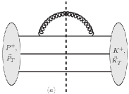
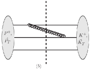
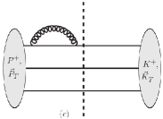
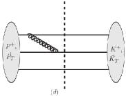
Figure 1: Diagrams for the computation of the proton wave function normalization at $\mathcal{O}(g^{2})$. In figures the notation ${\vec{K}}={\vec{K}}_{T}$ is used.

The $\mathcal{O}(g^{2})$ corrections to $\langle K|P\rangle$ are depicted in fig. 1. For diagram 1(a) we get

$$\begin{split}\langle K|P\rangle_{\mathrm{fig}.~{}\ref{fig:Norm_g2}(a)}&=(2\pi)^{3}\,P^{+}\delta(P^{+}-K^{+})\,\delta({\vec{P}}-{\vec{K}})\int[\,\mathrm{d}x_{i}]\int[\,\mathrm{d}^{2}k_{i}]\,\,\frac{1}{2p_{1}^{+}}\int{\widetilde{\mathrm{d}k}}_{g}\frac{1}{2(p_{1}^{+}-k_{g}^{+})}\left|\psi_{q\to qg}(p_{1};p_{1}-k_{g},k_{g})\right|^{2}\\ &\hskip 142.26378pt|\Psi_{qqq}(x_{1},{\vec{k}}_{1};x_{2},{\vec{k}}_{2};x_{3},{\vec{k}}_{3})|^{2}\,\langle S|S\rangle\\ &=(2\pi)^{3}\,P^{+}\delta(P^{+}-K^{+})\,\delta({\vec{P}}-{\vec{K}})\int[\,\mathrm{d}x_{i}]\int[\,\mathrm{d}^{2}k_{i}]\,\,C_{q}(p_{1}^{+})\,|\Psi_{qqq}(x_{1},{\vec{k}}_{1};x_{2},{\vec{k}}_{2};x_{3},{\vec{k}}_{3})|^{2}\,\langle S|S\rangle~{}.\end{split}$$ (47)

This diagram has a symmetry factor of 3 since the gluon may also be emitted and reabsorbed by quarks 2 or 3.

For diagram 1(c) we get

$$\begin{split}\langle K|P\rangle_{\mathrm{fig}.~{}\ref{fig:Norm_g2}(c)}&=-(2\pi)^{3}\,P^{+}\delta(P^{+}-K^{+})\,\delta({\vec{P}}-{\vec{K}})\int[\,\mathrm{d}x_{i}]\int[\,\mathrm{d}^{2}k_{i}]\,\,\frac{C_{q}(p_{1}^{+})}{2}\,|\Psi_{qqq}(x_{1},{\vec{k}}_{1};x_{2},{\vec{k}}_{2};x_{3},{\vec{k}}_{3})|^{2}\,\langle S|S\rangle~{}.\end{split}$$ (48)

This will be multiplied by a symmetry factor of 6. These two UV divergent contributions cancel.

Continuing to diagram 1(b) we find

$$\begin{split}\langle K|P\rangle_{\mathrm{fig}.~{}\ref{fig:Norm_g2}(b)}&=-16\pi^{3}\,P^{+}\delta(P^{+}-K^{+})\,\delta({\vec{P}}-{\vec{K}})\\ &\frac{g^{2}C_{F}N_{c}}{12}\int[\,\mathrm{d}x_{i}]\int[\,\mathrm{d}^{2}k_{i}]\Psi_{qqq}(x_{1},{\vec{k}}_{1};x_{2},{\vec{k}}_{2};x_{3},{\vec{k}}_{3})\int\frac{{\widetilde{\mathrm{d}k}}_{g}}{p_{1}^{+}-k_{g}^{+}}\frac{1}{p_{2}^{+}+k_{g}^{+}}\\ &\Psi^{*}_{qqq}(x_{1}-x_{g},{\vec{k}}_{1}-{\vec{k}}_{g}+x_{g}{\vec{P}};x_{2}+x_{g},{\vec{k}}_{2}+{\vec{k}}_{g}-x_{g}{\vec{P}};x_{3},{\vec{k}}_{3})\\ &\langle S|\hat{\psi}_{q\to qg}(p_{1};p_{1}-k_{g},k_{g})\,\hat{\psi}_{q\to qg}^{*}(p_{2}+k_{g};p_{2},k_{g})\,|S\rangle~{}.\end{split}$$ (49)

Note that the summations over the polarization of the gluon and the helicities of the daughter quarks are not indicated; the helicities $h_{1},h_{2}$ of the parent quarks which appear in the $q\to qg$ amplitudes are those from $|S\rangle$. Also, there is an upper limit for the integration over $k_{g}^{+}$ which is given by min($p_{1}^{+},P^{+}-p_{2}^{+}$).

The integral over ${\vec{k}}_{g}$ converges in the UV because it shifts the arguments of $\Psi^{*}_{qqq}$. Therefore, we can immediately insert the $D=4$ form of $\psi_{q\to qg}$ from eq. (29):

$$\begin{split}\frac{\hat{\psi}_{q\to qg}(p_{1};p_{1}-k_{g},k_{g})\,\hat{\psi}_{q\to qg}^{*}(p_{2}+k_{g};p_{2},k_{g})}{4p_{1}^{+}(p_{2}^{+}+k_{g}^{+})\sqrt{1-z_{1}}\sqrt{1-z_{2}}}&=\left[\left(1-\frac{z_{1}}{2}\right)\delta^{ij}+\frac{z_{1}}{2}ih_{1}\epsilon^{ij}\right]\left[\left(1-\frac{z_{2}}{2}\right)\delta^{kl}-\frac{z_{2}}{2}ih_{2}\epsilon^{kl}\right]\delta^{jl}\\ &~{}~{}~{}\,\frac{(k_{g}^{i}-z_{1}p_{1}^{i})}{({\vec{k}}_{g}-z_{1}{\vec{p}}_{1})^{2}}\frac{((1-z_{2})k_{g}^{k}-z_{2}p_{2}^{k})}{((1-z_{2}){\vec{k}}_{g}-z_{2}{\vec{p}}_{2})^{2}}\\ &=\left[\left(\left(1-\frac{z_{1}}{2}\right)\left(1-\frac{z_{2}}{2}\right)+\frac{z_{1}z_{2}}{4}h_{1}h_{2}\right)\delta^{ik}+\left(ih_{1}\frac{z_{1}}{2}\left(1-\frac{z_{2}}{2}\right)-ih_{2}\frac{z_{2}}{2}\left(1-\frac{z_{1}}{2}\right)\right)\epsilon^{ik}\right]\\ &~{}~{}~{}~{}\frac{(k_{g}^{i}-z_{1}p_{1}^{i})}{({\vec{k}}_{g}-z_{1}{\vec{p}}_{1})^{2}}\frac{((1-z_{2})k_{g}^{k}-z_{2}p_{2}^{k})}{((1-z_{2}){\vec{k}}_{g}-z_{2}{\vec{p}}_{2})^{2}}~{},\end{split}$$ (50)

where $z_{1}=\frac{x_{g}}{x_{1}}$ and $z_{2}=\frac{x_{g}}{x_{2}+x_{g}}$. We now have to sandwich this expression between proton helicity states as given in eq. (19). Note that $h_{1}=\uparrow$ and $h_{1}=\downarrow$ occur an equal number of times (same for $h_{2}$) so that terms linear in helicity drop out, while $\langle S|h_{1}h_{2}|S\rangle=-\frac{1}{3}$ (incl. symmetrization over permutations of quark helicities, c.f. sec. II.1). Hence,

$$\begin{split}\langle S|\hat{\psi}_{q\to qg}(p_{1};p_{1}-k_{g},k_{g})\,\hat{\psi}_{q\to qg}^{*}(p_{2}+k_{g};p_{2},k_{g})\,|S\rangle&=4p_{1}^{+}(p_{2}^{+}+k_{g}^{+})\sqrt{1-z_{1}}\sqrt{1-z_{2}}\left(1-\frac{z_{1}+z_{2}}{2}+\frac{z_{1}z_{2}}{6}\right)\\ &~{}~{}~{}\frac{({\vec{k}}_{g}-z_{1}{\vec{p}}_{1})}{({\vec{k}}_{g}-z_{1}{\vec{p}}_{1})^{2}}\cdot\frac{((1-z_{2}){\vec{k}}_{g}-z_{2}{\vec{p}}_{2})}{((1-z_{2}){\vec{k}}_{g}-z_{2}{\vec{p}}_{2})^{2}}~{}.\end{split}$$ (51)

With this we finally obtain

$$\begin{split}\langle K|P\rangle_{\mathrm{fig}.~{}\ref{fig:Norm_g2}(b)}&=-16\pi^{3}\,P^{+}\delta(P^{+}-K^{+})\,\delta({\vec{P}}-{\vec{K}})\\ &g^{2}C_{F}\int[\,\mathrm{d}x_{i}]\int[\,\mathrm{d}^{2}k_{i}]\Psi_{qqq}(x_{1},{\vec{k}}_{1};x_{2},{\vec{k}}_{2};x_{3},{\vec{k}}_{3})\int\limits^{\mathrm{min}(x_{1},1-x_{2})}_{x}\frac{\,\mathrm{d}x_{g}}{x_{g}}\frac{x_{1}}{x_{1}-x_{g}}\int\frac{\,\mathrm{d}^{2}k_{g}}{16\pi^{3}}\\ &\Psi^{*}_{qqq}(x_{1}-x_{g},{\vec{k}}_{1}-{\vec{k}}_{g}+x_{g}{\vec{P}};x_{2}+x_{g},{\vec{k}}_{2}+{\vec{k}}_{g}-x_{g}{\vec{P}};x_{3},{\vec{k}}_{3})\\ &\sqrt{1-z_{1}}\sqrt{1-z_{2}}\left(1-\frac{z_{1}+z_{2}}{2}+\frac{z_{1}z_{2}}{6}\right)\,\frac{({\vec{k}}_{g}-z_{1}{\vec{p}}_{1})}{({\vec{k}}_{g}-z_{1}{\vec{p}}_{1})^{2}}\cdot\frac{((1-z_{2}){\vec{k}}_{g}-z_{2}{\vec{p}}_{2})}{((1-z_{2}){\vec{k}}_{g}-z_{2}{\vec{p}}_{2})^{2}}~{}.\end{split}$$ (52)

Recall that $z_{1}=\frac{x_{g}}{x_{1}}$, $z_{2}=\frac{x_{g}}{x_{2}+x_{g}}$ and ${\vec{p}}_{1,2}={\vec{k}}_{1,2}+x_{1,2}{\vec{P}}$; the shift ${\vec{k}}_{g}\to{\vec{k}}_{g}+x_{g}{\vec{P}}$ makes this expression independent of ${\vec{P}}$. Here, $x$ is the minimal allowed LC momentum fraction of the gluon, i.e. in subsequent sections we will evaluate correlators of color charges with LC momenta greater than $xP^{+}$. In eq. (52) the first quark emits and the second quark absorbs the gluon. By symmetry of the wave function $\Psi_{qqq}$ under exchange of the quarks, reversing emission and absorption leads to the same result. Also, thanks to the fact that we have averaged over permutations of the helicities of the three quarks, in all we can simply multiply this diagram by a symmetry factor of 6 to include the contributions where quarks 1 and 3 or quarks 2 and 3 exchange the gluon.

Lastly,

$$\begin{split}\langle K|P\rangle_{\mathrm{fig}.~{}\ref{fig:Norm_g2}(d)}&=-16\pi^{3}\,P^{+}\delta(P^{+}-K^{+})\,\delta({\vec{P}}-{\vec{K}})\\ &\frac{g^{2}C_{F}N_{c}}{12}\int[\,\mathrm{d}x_{i}]\int[\,\mathrm{d}^{2}k_{i}]\Psi_{qqq}(x_{1},{\vec{k}}_{1};x_{2},{\vec{k}}_{2};x_{3},{\vec{k}}_{3})\int\frac{{\widetilde{\mathrm{d}k}}_{g}}{p_{1}^{+}-k_{g}^{+}}\frac{1}{p_{2}^{+}+k_{g}^{+}}\\ &\Psi^{*}_{qqq}(x_{1}-x_{g},{\vec{k}}_{1}-{\vec{k}}_{g}+x_{g}{\vec{P}};x_{2}+x_{g},{\vec{k}}_{2}+{\vec{k}}_{g}-x_{g}{\vec{P}};x_{3},{\vec{k}}_{3})\\ &\langle S|\hat{\psi}_{q\to qg}(p_{1};p_{1}-k_{g},k_{g})\,\hat{\psi}_{qg\to q}(p_{2},k_{g};p_{2}+k_{g})\,|S\rangle~{}.\end{split}$$ (53)

Here, the product

$$\begin{split}\langle S|\hat{\psi}_{q\to qg}(p_{1};p_{1}-k_{g},k_{g})\,\hat{\psi}_{qg\to q}(p_{2},k_{g};p_{2}+k_{g})\,|S\rangle&=-4p_{1}^{+}(p_{2}^{+}+k_{g}^{+})\sqrt{1-z_{1}}\sqrt{1-z_{2}}\left(1-\frac{z_{1}+z_{2}}{2}+\frac{z_{1}z_{2}}{6}\right)\\ &~{}~{}~{}\frac{({\vec{k}}_{g}-z_{1}{\vec{p}}_{1})}{({\vec{k}}_{g}-z_{1}{\vec{p}}_{1})^{2}}\cdot\frac{((1-z_{2}){\vec{k}}_{g}-z_{2}{\vec{p}}_{2})}{((1-z_{2}){\vec{k}}_{g}-z_{2}{\vec{p}}_{2})^{2}}~{},\end{split}$$ (54)

where $z_{1}=k_{g}^{+}/p_{1}^{+}=x_{g}/x_{1}$ and $z_{2}=k_{g}^{+}/(p_{2}^{+}+k_{g}^{+})=x_{g}/(x_{2}+x_{g})$. Therefore, we find the result

$$\begin{split}\langle K|P\rangle_{\mathrm{fig}.~{}\ref{fig:Norm_g2}(d)}&=16\pi^{3}\,P^{+}\delta(P^{+}-K^{+})\,\delta({\vec{P}}-{\vec{K}})\\ &g^{2}C_{F}\int[\,\mathrm{d}x_{i}]\int[\,\mathrm{d}^{2}k_{i}]\Psi_{qqq}(x_{1},{\vec{k}}_{1};x_{2},{\vec{k}}_{2};x_{3},{\vec{k}}_{3})\int\limits^{\mathrm{min}(x_{1},1-x_{2})}_{x}\frac{\,\mathrm{d}x_{g}}{x_{g}}\frac{x_{1}}{x_{1}-x_{g}}\int\frac{\,\mathrm{d}^{2}k_{g}}{16\pi^{3}}\\ &\Psi^{*}_{qqq}(x_{1}-x_{g},{\vec{k}}_{1}-{\vec{k}}_{g}+x_{g}{\vec{P}};x_{2}+x_{g},{\vec{k}}_{2}+{\vec{k}}_{g}-x_{g}{\vec{P}};x_{3},{\vec{k}}_{3})\\ &\sqrt{1-z_{1}}\sqrt{1-z_{2}}\left(1-\frac{z_{1}+z_{2}}{2}+\frac{z_{1}z_{2}}{6}\right)\frac{({\vec{k}}_{g}-z_{1}{\vec{p}}_{1})}{({\vec{k}}_{g}-z_{1}{\vec{p}}_{1})^{2}}\cdot\frac{((1-z_{2}){\vec{k}}_{g}-z_{2}{\vec{p}}_{2})}{((1-z_{2}){\vec{k}}_{g}-z_{2}{\vec{p}}_{2})^{2}}~{}.\end{split}$$ (55)

The shift ${\vec{k}}_{g}\to{\vec{k}}_{g}+x_{g}{\vec{P}}$ again shows that this expression is in fact independent of ${\vec{P}}$.

The symmetry factor for this diagram is $\frac{1}{2}\times 12=6$. Hence, the diagrams in fig. 1(d), eq. (55), and in fig. 1(b), eq. (52), also cancel. The normalization condition for $\Psi_{qqq}$ therefore remains as written in eq. (12).

IV Color charge correlators

IV.1 Color charge operators

The color charge operator $\rho^{a}(\vec{x})$ measures the color charge density at transverse coordinate $\vec{x}$, integrated over the longitudinal coordinate $x^{-}$. Its 2d Fourier transform is $\rho^{a}(\vec{k})$. The contribution to this Fock space operator due to quarks is given by the plus component of their color current $g(t^{a})_{ij}\bar{\psi}_{i}\gamma^{+}\psi_{j}$ Dumitru et al. (2018),

$$\rho^{a}_{\mathrm{qu}}(\vec{k})=g\sum_{i,j,\sigma}(t^{a})_{ij}\int\frac{{\rm d}x_{q}{\rm d}^{2}q}{16\pi^{3}\,x_{q}}b^{\dagger}_{i\sigma}(x_{q},\vec{q})\,b_{j\sigma}(x_{q},\vec{k}+\vec{q})~{},$$ (56)

where $t^{a}$ are the generators of the fundamental representation of color-SU(3).

The contribution of gluons to the color current in light-cone gauge is (see, for example, ref. Burkardt (2004))

$$J^{+a}_{\mathrm{gl}}(x)=gf^{abc}A^{ib}(x)\,\partial^{+}A^{ic}(x)~{},$$ (57)

with $\partial^{+}=\partial_{-}=\frac{\partial}{\partial x^{-}}$. This follows from the quadratic in $A^{i}$ part of $(D_{\nu})^{ab}\,(F^{\nu+})^{b}=J^{+a}_{\mathrm{qu}}$ which we shift to the r.h.s. of the equation. Using $(D_{\nu})_{ab}=\delta_{ab}\partial_{\nu}+igA_{\nu}^{c}(T^{c})_{ab}$ and $F^{-+}_{b}=0$ we obtain $J^{+a}_{\mathrm{gl}}(x)=igA^{ic}(T^{c})^{ab}F^{i+b}$ with $F^{i+}_{b}=-\partial_{-}A^{i}_{b}$. $(T^{c})^{ab}=-if^{cab}$ are the generators of the adjoint representation of color-SU(3).

Next we introduce the standard plane wave expansion of the bare gluon field in LC gauge on the $x^{+}=0$ front:

$$A^{ia}(x^{-},\vec{x})=\sum_{\lambda}\int\frac{{\rm d}k^{+}{\rm d}^{2}k}{16\pi^{3}\,k^{+}}\left[\epsilon^{i}_{\lambda}a_{a\lambda}(k)e^{-ik\cdot x}+\epsilon^{*i}_{\lambda}a^{\dagger}_{a\lambda}(k)e^{ik\cdot x}\right]\Bigg{|}_{x^{+}=0}~{}.$$ (58)

Integrating $J^{+}$ over $x^{-}$ leads to

$$\rho_{\mathrm{gl}}^{a}(\vec{x})=2\pi igf^{abc}\sum_{\lambda bc}\int\frac{{\rm d}k^{+}{\rm d}^{2}k}{16\pi^{3}\,k^{+}}\int\frac{{\rm d}\ell^{+}{\rm d}^{2}\ell}{16\pi^{3}\,\ell^{+}}\ell^{+}\delta(k^{+}-\ell^{+})\left[a_{b\lambda}(k)\,a^{\dagger}_{c\lambda}(\ell)e^{i(\vec{k}-\vec{\ell})\cdot\vec{x}}-a^{\dagger}_{b\lambda}(k)\,a_{c\lambda}(\ell)e^{-i(\vec{k}-\vec{\ell})\cdot\vec{x}}\right]~{}.$$ (59)

Here, $a_{b\lambda}(k)\,a^{\dagger}_{c\lambda}(\ell)$ can be replaced by $a^{\dagger}_{c\lambda}(\ell)\,a_{b\lambda}(k)$ because the commutator is proportional to $\delta_{bc}$, eq. (13). Finally, performing a Fourier transform to transverse momentum space we find

$$\rho_{\mathrm{gl}}^{a}(\vec{k})=g\sum_{\lambda bc}(T^{a})_{bc}\int\frac{{\rm d}x_{g}{\rm d}^{2}q}{16\pi^{3}\,x_{g}}a^{\dagger}_{b\lambda}(x_{g},\vec{q})\,a_{c\lambda}(x_{g},\vec{q}+\vec{k})~{}.$$ (60)

The eikonal currents formally sit at $x=0$ as we have integrated over $x^{-}$. They sum up the charge of all particles with LC momenta $>0$. However, as already discussed previously in sec. III.4, the integral over the L.C. momentum fraction $x_{g}$ of the gluon diverges at $x_{g}\to 0$, and so we introduce a cut off $x$ to exclude gluon fluctuations with $x_{g}<x$. Hence, our proton does not “contain” any gluons below $x$ so that, in effect, the correlator $\langle\rho^{a}\,\rho^{b}\rangle$ which we compute below excludes contributions from softer gluons. It would make no difference in our analysis if our $\rho^{a}(q)$ sat at non-zero $q^{+}$, as long as this $q^{+}$ is less than $xP^{+}$. In other words, we work in the “shockwave” limit where there exists a separation of scales such that the plus momentum of the gluon fluctuations in the proton exceeds that of the probes corresponding to the $\rho^{a}$ charge operators. In practical applications, one would choose the cutoff $x$ to correspond to the L.C. momentum fraction of color charges probed by the kinematics of the process.

IV.2 Correlator of two color charge operators, $\langle\rho^{a}(\vec{q}_{1})\,\rho^{b}(\vec{q}_{2})\rangle$

In this section we compute color charge correlations for two external probes, $\langle\rho^{a}(\vec{q}_{1})\,\rho^{b}(\vec{q}_{2})\rangle$. Since $\rho^{a}(\vec{q})=\rho^{a}_{\mathrm{qu}}(\vec{q})+\rho^{a}_{\mathrm{gl}}(\vec{q})$ we have

$$\langle\rho^{a}(\vec{q}_{1})\,\rho^{b}(\vec{q}_{2})\rangle=\langle\rho^{a}_{\mathrm{gl}}(\vec{q}_{1})\,\rho^{b}_{\mathrm{gl}}(\vec{q}_{2})\rangle+\langle\rho^{a}_{\mathrm{gl}}(\vec{q}_{1})\,\rho^{b}_{\mathrm{qu}}(\vec{q}_{2})\rangle+\langle\rho^{a}_{\mathrm{qu}}(\vec{q}_{1})\,\rho^{b}_{\mathrm{gl}}(\vec{q}_{2})\rangle+\langle\rho^{a}_{\mathrm{qu}}(\vec{q}_{1})\,\rho^{b}_{\mathrm{qu}}(\vec{q}_{2})\rangle~{}.$$ (61)

We define expectation values of products of color charge operators by stripping off the delta functions for conservation of LC and transverse momentum:

$$\left<K|\rho^{a_{1}}(\vec{q}_{1})\cdots\rho^{a_{n}}(\vec{q}_{n})|P\right>=16\pi^{3}\,P^{+}\delta(P^{+}-K^{+})\,\,\delta\left(\vec{P}-\vec{K}-\sum_{i=1}^{n}\vec{q}_{i}\right)\,\left<\rho^{a_{1}}(\vec{q}_{1})\cdots\rho^{a_{n}}(\vec{q}_{n})\right>.$$ (62)

It is understood that the color charge correlators correspond to a transverse momentum of the scattered proton of $\vec{K}=\vec{P}-\sum\vec{q}_{i}$ and light-cone momentum $K^{+}=P^{+}$. We will also abbreviate $\vec{q}=\sum_{i=1}^{n}\vec{q}_{i}$.

IV.2.1 Coupling to gluon, $\langle\rho^{a}_{\mathrm{gl}}(\vec{q}_{1})\,\rho^{b}_{\mathrm{gl}}(\vec{q}_{2})\rangle$

We begin with the diagrams where both external probes couple to the gluon in the proton. (We amputate the propagators of the external gluons in the following diagrams to obtain the expectation value of the color charge correlator.)

      

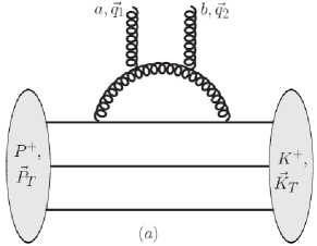
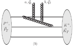
Figure 2: Diagrams for $\langle\rho^{b}_{\mathrm{gl}}(\vec{q}_{2})\,\rho^{a}_{\mathrm{gl}}(\vec{q}_{1})\rangle$. The cut is located at the insertion of the two color charge operators.

To prepare, we first compute the matrix element of $\rho^{a}_{\mathrm{gl}}(\vec{q}_{1})\,\rho^{b}_{\mathrm{gl}}(\vec{q}_{2})$ between one-gluon states:

$$\left<\ell,\rho,d|\,\rho^{a}_{\mathrm{gl}}(\vec{q}_{1})\,\rho^{b}_{\mathrm{gl}}(\vec{q}_{2})\,|k_{g},\sigma,c\right>=g^{2}\left(T^{a}T^{b}\right)_{dc}\,\delta_{\rho\sigma}\,(2\pi)^{D-1}\,2k_{g}^{+}\delta(k_{g}^{+}-\ell^{+})\,\delta(\vec{k}_{g}-\vec{\ell}-\vec{q})~{}.$$ (63)

Here we used the color charge operator from eq. (60) and the commutation relations (13).

We now proceed to compute fig.2a which reads

$$\left<K|\rho^{a}_{\mathrm{gl}}(\vec{q}_{1})\,\rho^{b}_{\mathrm{gl}}(\vec{q}_{2})|P\right> = \frac{4g^{2}}{6}\int[{\rm d}x_{i}]\int[{\rm d}^{2}k_{i}]\,\Psi_{qqq}(x_{i},\vec{k}_{i})\,\epsilon_{i_{1}i_{2}i_{3}}\int[{\rm d}x_{i}^{\prime}]\int[{\rm d}^{2}k_{i}^{\prime}]\,\Psi_{qqq}^{*}(x_{i}^{\prime},\vec{k}_{i}^{\prime})\,\epsilon_{i_{1}^{\prime}i_{2}^{\prime}i_{3}^{\prime}}\,(t^{c})_{ji_{1}}(t^{d})_{i_{1}^{\prime}j^{\prime}}$$ (64)

$$\int\frac{{\widetilde{\mathrm{d}k}}_{g}}{2(p_{1}^{+}-k_{g}^{+})}\int\frac{{\widetilde{\mathrm{d}k}}_{g}^{\prime}}{2(p_{1}^{+\prime}-k_{g}^{+\prime})}\langle S|\hat{\psi}_{q\to qg}(p_{1};p_{1}-k_{g},k_{g})\hat{\psi}_{q\to qg}^{*}(p_{1}^{\prime};p_{1}^{\prime}-k_{g}^{\prime},k_{g}^{\prime})|S\rangle$$

$$\langle p_{2}^{\prime},i_{2}^{\prime}|p_{2},i_{2}\rangle\,\langle p_{3}^{\prime},i_{3}^{\prime}|p_{3},i_{3}\rangle\,\langle p_{1}^{\prime}-k_{g}^{\prime},j^{\prime}|p_{1}-k_{g},j\rangle\,\left<k_{g}^{\prime},d|\,\rho^{a}_{\mathrm{gl}}(\vec{q}_{1})\,\rho^{b}_{\mathrm{gl}}(\vec{q}_{2})\,|k_{g},c\right>~{}.$$

Here, $p_{i}$ are the momenta of the quarks in $|P\rangle$ (with $p_{i}^{+}=x_{i}P^{+}$ and $\vec{p}_{i}=\vec{k}_{i}+x_{i}\vec{P}$), and $p_{i}^{\prime}$ those of the quarks in $\langle K|$ (with $p_{i}^{+\prime}=x_{i}^{\prime}K^{+}$ and $\vec{p}_{i}^{\prime}=\vec{k}_{i}^{\prime}+x_{i}^{\prime}\vec{K}$).

If we now evaluate the quark state overlaps and insert the result (63) we obtain

$$\mathrm{fig.}\,\ref{fig:rho-rho_gl}\mathrm{a} = \frac{2g^{4}}{3\cdot 16\pi^{3}}\,\,\mathrm{tr}\,T^{a}T^{b}\int\left[{\rm d}x_{i}\right]\int\left[{\rm d}^{2}k_{i}\right]\,\Psi_{qqq}(x_{1},\vec{k}_{1};x_{2},\vec{k}_{2};x_{3},\vec{k}_{3})\,$$ (65)

$$\Psi_{qqq}^{*}(x_{1},\vec{k}_{1}-(1-x_{1})\vec{q};x_{2},\vec{k}_{2}+x_{2}\vec{q};x_{3},\vec{k}_{3}+x_{3}\vec{q})$$

$$\frac{(2\pi)^{D-1}}{2p_{1}^{+}}\int\frac{{\widetilde{\mathrm{d}k}}_{g}}{2(p_{1}^{+}-k_{g}^{+})}\langle S|\hat{\psi}_{q\to qg}(p_{1};p_{1}-k_{g},k_{g})\,\hat{\psi}^{*}_{q\to qg}(p_{1}-q;p_{1}-k_{g},k_{g}-q)|S\rangle~{},$$

where $\,\mathrm{tr}\,T^{a}T^{b}=N_{c}\,\delta^{ab}$. Also, recall that the plus component of $\vec{q}_{1},\vec{q}_{2}$ is zero. The symmetry factor for this diagram is 3. The expression for the integral of $\hat{\psi}_{q\to qg}\,\hat{\psi}^{*}_{q\to qg}$ over $k_{g}$ is given in eq. (43) above.

For fig.2b we get

$$\left<K|\rho^{a}_{\mathrm{gl}}(\vec{q}_{1})\,\rho^{b}_{\mathrm{gl}}(\vec{q}_{2})|P\right> = \frac{4g^{2}}{6}\int[{\rm d}x_{i}]\int[{\rm d}^{2}k_{i}]\,\Psi_{qqq}(x_{i},\vec{k}_{i})\epsilon_{i_{1}i_{2}i_{3}}\int[{\rm d}x_{i}^{\prime}]\int[{\rm d}^{2}k_{i}^{\prime}]\,\Psi_{qqq}^{*}(x_{i}^{\prime},\vec{k}_{i}^{\prime})\epsilon_{i_{1}^{\prime}i_{2}^{\prime}i_{3}^{\prime}}$$ (67)

$$\int\frac{{\widetilde{\mathrm{d}k}}_{g}}{2(p_{1}^{+}-k_{g}^{+})}\frac{{\widetilde{\mathrm{d}k}}_{g}^{\prime}}{2(p_{2}^{+\prime}-k_{g}^{+\prime})}\langle S|\hat{\psi}_{q\to qg}(p_{1};p_{1}-k_{g},k_{g})\hat{\psi}_{q\to qg}^{*}(p_{2}^{\prime};p_{2}^{\prime}-k_{g}^{\prime},k_{g}^{\prime})|S\rangle$$

$$\langle p_{3}^{\prime},i_{3}^{\prime}|p_{3},i_{3}\rangle\,\langle p_{1}^{\prime},i_{1}^{\prime}|p_{1}-k_{g},j_{1}\rangle\,\langle p_{2}^{\prime}-k_{g}^{\prime},j_{2}|p_{2},i_{2}\rangle$$

$$\left<k_{g}^{\prime},d|\,\rho^{a}_{\mathrm{gl}}(\vec{q}_{1})\,\rho^{b}_{\mathrm{gl}}(\vec{q}_{2})\,|k_{g},c\right>\,(t^{c})_{j_{1}i_{1}}\,(t^{d})_{i_{2}^{\prime}j_{2}}$$

$$= -\frac{g^{4}}{6}\mathrm{tr}\,T^{a}T^{b}\,P^{+}\delta(P^{+}-K^{+})\,\delta(\vec{P}-\vec{K}-\vec{q})$$

$$\int[{\rm d}x_{i}]\int[{\rm d}^{2}k_{i}]\,\Psi_{qqq}(x_{i},\vec{k}_{i})\int\frac{{\rm d}k_{g}^{+}}{k_{g}^{+}}\frac{{\rm d}^{2}k_{g}}{2(p_{1}^{+}-k_{g}^{+})}$$

$$\langle S|\hat{\psi}_{q\to qg}(p_{1};p_{1}-k_{g},k_{g})\hat{\psi}_{q\to qg}^{*}(p_{2}+k_{g}-q;p_{2},k_{g}-q)|S\rangle\,\frac{x_{2}}{x_{2}+x_{g}}\frac{1}{2p_{2}^{+}}$$

$$\Psi_{qqq}^{*}(x_{1}-x_{g},\vec{k}_{1}+x_{1}\vec{q}-\vec{k}_{g}+x_{g}\vec{K};x_{2}+x_{g},\vec{k}_{2}-(1-x_{2})\vec{q}+\vec{k}_{g}-x_{g}\vec{K};x_{3},\vec{k}_{3}+x_{3}\vec{q})~{}.$$

We again evaluate the helicity matrix element of $\hat{\psi}_{q\to qg}\hat{\psi}_{q\to qg}^{*}$ as in eq. (51). This leads to the finite result

$$\mathrm{fig.}\,\ref{fig:rho-rho_gl}\mathrm{b} = -\frac{g^{4}}{6\cdot 16\pi^{3}}\,\,\mathrm{tr}\,T^{a}T^{b}\int\left[{\rm d}x_{i}\right]\int\left[{\rm d}^{2}k_{i}\right]\,\Psi_{qqq}(x_{1},\vec{k}_{1};x_{2},\vec{k}_{2};x_{3},\vec{k}_{3})\,$$ (68)

$$\int\limits_{x}^{\mathrm{min}(x_{1},1-x_{2})}\frac{{\rm d}x_{g}}{x_{g}}\int{\rm d}^{2}k_{g}\frac{z_{1}\vec{p}_{1}-\vec{k}_{g}}{\left(z_{1}\vec{p}_{1}-\vec{k}_{g}\right)^{2}}\cdot\frac{z_{2}\vec{p}_{2}-(1-z_{2})(\vec{k}_{g}-\vec{q}_{1}-\vec{q}_{2})}{\left(z_{2}\vec{p}_{2}-(1-z_{2})(\vec{k}_{g}-\vec{q}_{1}-\vec{q}_{2})\right)^{2}}$$

$$\sqrt{\frac{x_{1}}{x_{1}-x_{g}}}\sqrt{\frac{x_{2}}{x_{2}+x_{g}}}\left(1-\frac{z_{1}+z_{2}}{2}+\frac{z_{1}z_{2}}{6}\right)$$

$$\Psi_{qqq}^{*}(x_{1}-x_{g},\vec{k}_{1}+x_{1}\vec{q}-\vec{k}_{g}+x_{g}\vec{K};x_{2}+x_{g},\vec{k}_{2}-(1-x_{2})\vec{q}+\vec{k}_{g}-x_{g}\vec{K};x_{3},\vec{k}_{3}+x_{3}\vec{q})~{},$$

with $z_{1}=x_{g}/x_{1}$ and $z_{2}=x_{g}/(x_{2}+x_{g})$. Here, the symmetry factor is 6 which includes a factor of 2 for interchanging the gluon emission and absorption vertices between quarks 1 and 2. Note that this expression is invariant under translations in 2d transverse momentum space corresponding to a constant shift of both $\vec{P}$ and $\vec{K}$; this is evident upon shifting the integration variable $\vec{k}_{g}\to\vec{k}_{g}+x_{g}\vec{K}$.

IV.2.2 Coupling to one quark and the gluon, $\langle\rho^{a}_{\mathrm{qu}}(\vec{q}_{1})\,\rho^{b}_{\mathrm{gl}}(\vec{q}_{2})\rangle$

In this section we compute $\langle\rho^{a}_{\mathrm{qu}}(\vec{q}_{1})\,\rho^{b}_{\mathrm{gl}}(\vec{q}_{2})\rangle$. We can then obtain $\langle\rho^{a}_{\mathrm{gl}}(\vec{q}_{1})\,\rho^{b}_{\mathrm{qu}}(\vec{q}_{2})\rangle$ simply by exchanging $a\leftrightarrow b$, $\vec{q}_{1}\leftrightarrow\vec{q}_{2}$ since the two charge operators commute.

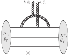
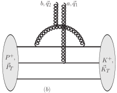
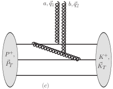
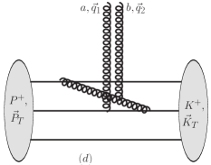
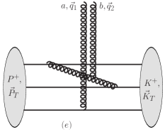
Figure 3: Diagrams for $\langle\rho^{a}_{\mathrm{qu}}(\vec{q}_{1})\,\rho^{b}_{\mathrm{gl}}(\vec{q}_{2})\rangle$.

To prepare this calculation, we first list the matrix elements of $\rho^{a}_{\mathrm{qu}}(\vec{q})$ and $\rho^{a}_{\mathrm{gl}}(\vec{q})$ between one quark and one gluon states, respectively:

$$\begin{split}\left<k,h^{\prime},i^{\prime}|\,\rho^{a}_{\mathrm{qu}}(\vec{q})\,|p,h,i\right>&=g\,(t^{a})_{i^{\prime}i}\,16\pi^{3}\,\delta_{h^{\prime}h}\,p^{+}\delta(p^{+}-k^{+})\,\delta(\vec{p}-\vec{k}-\vec{q})~{},\\ \left<k,\rho,b|\,\rho^{a}_{\mathrm{gl}}(\vec{q})\,|p,\sigma,c\right>&=g(T^{a})_{bc}\,(2\pi)^{D-1}\,\delta_{\rho\sigma}\,2p^{+}\delta(p^{+}-k^{+})\,\delta(\vec{p}-\vec{k}-\vec{q})~{}.\end{split}$$ (69)

We then obtain

$$\mathrm{fig.}\,\ref{fig:rho-rho_qu-gl}\mathrm{a} = -\frac{g^{4}}{3\cdot 16\pi^{3}}\,\,\mathrm{tr}\,T^{a}T^{b}\int\left[{\rm d}x_{i}\right]\int\left[{\rm d}^{2}k_{i}\right]\,\Psi_{qqq}(x_{1},\vec{k}_{1};x_{2},\vec{k}_{2};x_{3},\vec{k}_{3})\,$$ (70)

$$\Psi_{qqq}^{*}(x_{1},\vec{k}_{1}-(1-x_{1})\vec{q};x_{2},\vec{k}_{2}+x_{2}\vec{q};x_{3},\vec{k}_{3}+x_{3}\vec{q})$$

$$\frac{(2\pi)^{D-1}}{2p_{1}^{+}}\int\frac{{\widetilde{\mathrm{d}k}}_{g}}{2(p_{1}^{+}-k_{g}^{+})}\langle S|\hat{\psi}_{q\to qg}(p_{1};p_{1}-k_{g},k_{g})\,\hat{\psi}^{*}_{q\to qg}(p_{1}-q;p_{1}-k_{g}-q_{1},k_{g}-q_{2})|S\rangle~{}.$$

The symmetry factor is 3. Similarly,

$$\mathrm{fig.}\,\ref{fig:rho-rho_qu-gl}\mathrm{b} = -\frac{g^{4}}{6\cdot 16\pi^{3}}\,\,\mathrm{tr}\,T^{a}T^{b}\int\left[{\rm d}x_{i}\right]\int\left[{\rm d}^{2}k_{i}\right]\,\Psi_{qqq}(x_{1},\vec{k}_{1};x_{2},\vec{k}_{2};x_{3},\vec{k}_{3})\,$$ (71)

$$\Psi_{qqq}^{*}(x_{1},\vec{k}_{1}+x_{1}\vec{q}-\vec{q}_{2};x_{2},\vec{k}_{2}+x_{2}\vec{q}-\vec{q}_{1};x_{3},\vec{k}_{3}+x_{3}\vec{q})$$

$$\frac{(2\pi)^{D-1}}{2p_{1}^{+}}\int\frac{{\widetilde{\mathrm{d}k}}_{g}}{2(p_{1}^{+}-k_{g}^{+})}\langle S|\hat{\psi}_{q\to qg}(p_{1};p_{1}-k_{g},k_{g})\,\hat{\psi}^{*}_{q\to qg}(p_{1}-q_{2};p_{1}-k_{g},k_{g}-q_{2})|S\rangle~{}.$$

The symmetry factor is 6.

The remaining diagrams are finite.

$$\mathrm{fig.}\,\ref{fig:rho-rho_qu-gl}\mathrm{c} = \frac{g^{4}}{12\cdot 16\pi^{3}}\,\,\mathrm{tr}\,T^{a}T^{b}\int\left[{\rm d}x_{i}\right]\int\left[{\rm d}^{2}k_{i}\right]\,\Psi_{qqq}(x_{1},\vec{k}_{1};x_{2},\vec{k}_{2};x_{3},\vec{k}_{3})\,$$ (72)

$$\int\limits_{x}^{\mathrm{min}(x_{1},1-x_{2})}\frac{{\rm d}x_{g}}{x_{g}}\left(1-\frac{z_{1}+z_{2}}{2}+\frac{z_{1}z_{2}}{6}\right)\sqrt{\frac{x_{1}}{x_{1}-x_{g}}}\sqrt{\frac{x_{2}}{x_{2}+x_{g}}}$$

$$\int{\rm d}^{2}k_{g}\frac{z_{1}\vec{p}_{1}-\vec{k}_{g}}{\left(z_{1}\vec{p}_{1}-\vec{k}_{g}\right)^{2}}\cdot\frac{z_{2}\vec{p}_{2}-(1-z_{2})(\vec{k}_{g}-\vec{q}_{2})}{\left(z_{2}\vec{p}_{2}-(1-z_{2})(\vec{k}_{g}-\vec{q}_{2})\right)^{2}}$$

$$\Psi_{qqq}^{*}(x_{1}-x_{g},\vec{k}_{1}+x_{1}\vec{q}-\vec{q}_{1}-\vec{k}_{g}+x_{g}\vec{K};x_{2}+x_{g},\vec{k}_{2}+x_{2}\vec{q}-\vec{q}_{2}+\vec{k}_{g}-x_{g}\vec{K};x_{3},\vec{k}_{3}+x_{3}\vec{q})~{},$$

with the same $z_{1}$ and $z_{2}$ as above. The symmetry factor is 6.

$$\mathrm{fig.}\,\ref{fig:rho-rho_qu-gl}\mathrm{d} = \frac{g^{4}}{12\cdot 16\pi^{3}}\,\,\mathrm{tr}\,T^{a}T^{b}\int\left[{\rm d}x_{i}\right]\int\left[{\rm d}^{2}k_{i}\right]\,\Psi_{qqq}(x_{1},\vec{k}_{1};x_{2},\vec{k}_{2};x_{3},\vec{k}_{3})\,$$ (73)

$$\int\limits_{x}^{\mathrm{min}(x_{1},1-x_{2})}\frac{{\rm d}x_{g}}{x_{g}}\left(1-\frac{z_{1}+z_{2}}{2}+\frac{z_{1}z_{2}}{6}\right)\sqrt{\frac{x_{1}}{x_{1}-x_{g}}}\sqrt{\frac{x_{2}}{x_{2}+x_{g}}}$$

$$\int{\rm d}^{2}k_{g}\frac{z_{1}\vec{p}_{1}-\vec{k}_{g}}{\left(z_{1}\vec{p}_{1}-\vec{k}_{g}\right)^{2}}\cdot\frac{z_{2}(\vec{p}_{2}-\vec{q}_{1})-(1-z_{2})(\vec{k}_{g}-\vec{q}_{2})}{\left(z_{2}(\vec{p}_{2}-\vec{q}_{1})-(1-z_{2})(\vec{k}_{g}-\vec{q}_{2})\right)^{2}}$$

$$\Psi_{qqq}^{*}(x_{1}-x_{g},\vec{k}_{1}+x_{1}\vec{q}-\vec{k}_{g}+x_{g}\vec{K};x_{2}+x_{g},\vec{k}_{2}-(1-x_{2})\vec{q}+\vec{k}_{g}-x_{g}\vec{K};x_{3},\vec{k}_{3}+x_{3}\vec{q})~{},$$

The symmetry factor is 6.

$$\mathrm{fig.}\,\ref{fig:rho-rho_qu-gl}\mathrm{e} = 0$$ (74)

As already mentioned above, eqs. (70 - 73) should be duplicated with $\vec{q}_{1}\leftrightarrow\vec{q}_{2}$ to include the contribution from $\langle\rho^{a}_{\mathrm{gl}}(\vec{q}_{1})\,\rho^{b}_{\mathrm{qu}}(\vec{q}_{2})\rangle$.

IV.2.3 Coupling to quarks, $\langle\rho^{a}_{\mathrm{qu}}(\vec{q}_{1})\,\rho^{b}_{\mathrm{qu}}(\vec{q}_{2})\rangle$

Now consider the diagrams where both external probes couple to quarks. The matrix element of $\rho^{a}_{\mathrm{qu}}(\vec{q}_{1})\,\rho^{b}_{\mathrm{qu}}(\vec{q}_{2})$ in a one quark state is

$$\langle p^{\prime},j^{\prime}|\rho^{a}_{\mathrm{qu}}(\vec{q}_{1})\,\rho^{b}_{\mathrm{qu}}(\vec{q}_{2})|p,j\rangle=g^{2}(t^{a}t^{b})_{j^{\prime}j}\,16\pi^{3}\,p^{+}\,\delta(p^{\prime+}-p^{+})\,\delta(\vec{p}-\vec{p}^{\prime}-\vec{q})~{}.$$ (75)

The first contribution where the color charge operators are sandwiched between the bare 3-quark Fock states Dumitru et al. (2018) is

$$\langle\rho^{a}_{\mathrm{qu}}(\vec{q}_{1})\,\rho^{b}_{\mathrm{qu}}(\vec{q}_{2})\rangle = \frac{g^{2}}{6}\,\,\mathrm{tr}\,t^{a}t^{b}\,\int\left[{\rm d}x_{i}\right]\int\left[{\rm d}^{2}k_{i}\right]\,\Psi_{\mathrm{qqq}}(x_{1},\vec{k}_{1};x_{2},\vec{k}_{2};x_{3},\vec{k}_{3})$$ (76)

$$\left[\Psi_{\mathrm{qqq}}^{*}(x_{1},\vec{k}_{1}-(1-x_{1})\vec{q};x_{2},\vec{k}_{2}+x_{2}\vec{q};x_{3},\vec{k}_{3}+x_{3}\vec{q})\right.$$

$$-\frac{1}{2}\Psi_{\mathrm{qqq}}^{*}(x_{1},\vec{k}_{1}+x_{1}\vec{q}-\vec{q}_{1};x_{2},\vec{k}_{2}+x_{2}\vec{q}-\vec{q}_{2};x_{3},\vec{k}_{3}+x_{3}\vec{q})$$

$$-\left.\frac{1}{2}\Psi_{\mathrm{qqq}}^{*}(x_{1},\vec{k}_{1}+x_{1}\vec{q}-\vec{q}_{2};x_{2},\vec{k}_{2}+x_{2}\vec{q}-\vec{q}_{1};x_{3},\vec{k}_{3}+x_{3}\vec{q})\right]~{}.$$

The symmetry factor is 3. The first term (“handbag diagram”) is proportional to the quark GPD $\int{\rm d}x\,H_{q}(x,-\vec{q}^{2})$ at vanishing skewness; c.f. appendix B in ref. Burkardt (2003). The second and third terms (“cat’s ears diagrams”) are two-body diagrams where the gluon probes attach to different quarks in the proton. They ensure that the color charge correlator satisfies a Ward identity and vanishes when either $\vec{q}_{1}\to 0$ or $\vec{q}_{2}\to 0$. Also, these contributions are “higher twist” suppressed when both $q_{i}$ as well as $|\vec{q}_{1}-\vec{q}_{2}|$ are much greater than the typical transverse momentum of quarks in the 3-quark Fock state of the proton; on the other hand, the two-body contributions dominate when the two probes share a large momentum transfer, $\vec{q}_{1}\approx\vec{q}_{2}$, such as in exclusive $\gamma^{(*)}p\to J/\Psi\,p$ at large $-t$ Dumitru and Stebel (2019).

         

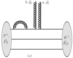
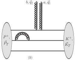
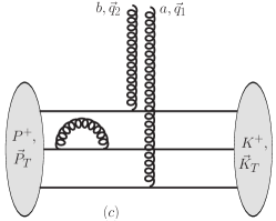
Figure 4: Some of the diagrams for the ${\cal O}(g^{2})$ correction to $\langle\rho^{a}_{\mathrm{qu}}(\vec{q}_{1})\,\rho^{b}_{\mathrm{qu}}(\vec{q}_{2})\rangle$ in the three-quark Fock state. The cut is located at the insertion of the two color charge operators.

To account for the quark wave function renormalization factor, we multiply the integrand in the previous equation by $Z_{q}(x_{1})\,Z_{q}(x_{2})\,Z_{q}(x_{3})=1-C_{q}(x_{1})-C_{q}(x_{2})-C_{q}(x_{3})$. This renormalization factor is given in eq. (42), where $\alpha\to x/x_{i}$. Some of the corresponding diagrams are shown in fig. 4.

              

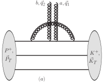
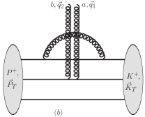
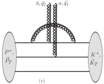
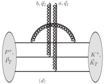
Figure 5: First set of diagrams for $\langle\rho^{a}_{\mathrm{qu}}(\vec{q}_{1})\,\rho^{b}_{\mathrm{qu}}(\vec{q}_{2})\rangle$. The cut is located at the insertion of the two color charge operators.

We now turn to the diagrams where $\rho^{a}_{\mathrm{qu}}(\vec{q}_{1})\,\rho^{b}_{\mathrm{qu}}(\vec{q}_{2})$ is sandwiched between $|qqqg\rangle$ Fock states or where two quarks exchange a gluon on either side of the operator insertion.

$$\mathrm{fig.}\,\ref{fig:rho-rho_qu}\mathrm{a} = \frac{4g^{4}C_{F}}{3\cdot 16\pi^{3}}\,\,\mathrm{tr}\,t^{a}t^{b}\int\left[{\rm d}x_{i}\right]\int\left[{\rm d}^{2}k_{i}\right]\,\Psi_{qqq}(x_{1},\vec{k}_{1};x_{2},\vec{k}_{2};x_{3},\vec{k}_{3})$$ (77)

$$\Psi_{qqq}^{*}(x_{1},\vec{k}_{1}-(1-x_{1})\vec{q};x_{2},\vec{k}_{2}+x_{2}\vec{q};x_{3},\vec{k}_{3}+x_{3}\vec{q})$$

$$\frac{(2\pi)^{D-1}}{2p_{1}^{+}}\int\frac{{\widetilde{\mathrm{d}k}}_{g}}{2(p_{1}^{+}-k_{g}^{+})}\langle S|\hat{\psi}_{q\to qg}(p_{1};p_{1}-k_{g},k_{g})\,\hat{\psi}^{*}_{q\to qg}(p_{1}-q;p_{1}-k_{g}-q,k_{g})|S\rangle~{}.$$

The symmetry factor is 3.

$$\mathrm{fig.}\,\ref{fig:rho-rho_qu}\mathrm{b} = \frac{4g^{4}C_{F}}{3\cdot 16\pi^{3}}\,\,\mathrm{tr}\,t^{a}t^{b}\int\left[{\rm d}x_{i}\right]\int\left[{\rm d}^{2}k_{i}\right]\,\Psi_{qqq}(x_{1},\vec{k}_{1};x_{2},\vec{k}_{2};x_{3},\vec{k}_{3})\,$$ (78)

$$\Psi_{qqq}^{*}(x_{1},\vec{k}_{1}+x_{1}\vec{q};x_{2},\vec{k}_{2}-(1-x_{2})\vec{q};x_{3},\vec{k}_{3}+x_{3}\vec{q})$$

$$\frac{(2\pi)^{D-1}}{2p_{1}^{+}}\int\frac{{\widetilde{\mathrm{d}k}}_{g}}{2(p_{1}^{+}-k_{g}^{+})}\langle S|\hat{\psi}_{q\to qg}(p_{1};p_{1}-k_{g},k_{g})\,\hat{\psi}^{*}_{q\to qg}(p_{1};p_{1}-k_{g},k_{g})|S\rangle~{}.$$

The symmetry factor is 6.

$$\mathrm{fig.}\,\ref{fig:rho-rho_qu}\mathrm{c} = \frac{2g^{4}}{3\cdot 6\cdot 16\pi^{3}}\,\,\mathrm{tr}\,t^{a}t^{b}\int\left[{\rm d}x_{i}\right]\int\left[{\rm d}^{2}k_{i}\right]\,\Psi_{qqq}(x_{1},\vec{k}_{1};x_{2},\vec{k}_{2};x_{3},\vec{k}_{3})\,$$ (79)

$$\Psi_{qqq}^{*}(x_{1},\vec{k}_{1}+x_{1}\vec{q}-\vec{q}_{2};x_{2},\vec{k}_{2}+x_{2}\vec{q}-\vec{q}_{1};x_{3},\vec{k}_{3}+x_{3}\vec{q})$$

$$\frac{(2\pi)^{D-1}}{2p_{1}^{+}}\int\frac{{\widetilde{\mathrm{d}k}}_{g}}{2(p_{1}^{+}-k_{g}^{+})}\langle S|\hat{\psi}_{q\to qg}(p_{1};p_{1}-k_{g},k_{g})\,\hat{\psi}^{*}_{q\to qg}(p_{1}-q_{2};p_{1}-k_{g}-q_{2},k_{g})|S\rangle~{}.$$

The symmetry factor is 6.

The diagram where the two probe gluons connect oppositely to quarks 1 and 2 is

$$\mathrm{fig.}\,\ref{fig:rho-rho_qu}\mathrm{c^{\prime}} = \mathrm{fig.}\,\ref{fig:rho-rho_qu}\mathrm{c}\,(\vec{q}_{1}\leftrightarrow\vec{q}_{2})$$ (80)

Again, the symmetry factor is 6.

Next,

$$\mathrm{fig.}\,\ref{fig:rho-rho_qu}\mathrm{d} = -\frac{2g^{4}C_{F}}{3\cdot 16\pi^{3}}\,\,\mathrm{tr}\,t^{a}t^{b}\int\left[{\rm d}x_{i}\right]\int\left[{\rm d}^{2}k_{i}\right]\,\Psi_{qqq}(x_{1},\vec{k}_{1};x_{2},\vec{k}_{2};x_{3},\vec{k}_{3})\,$$ (81)

$$\Psi_{qqq}^{*}(x_{1},\vec{k}_{1}+x_{1}\vec{q};x_{2},\vec{k}_{2}+x_{2}\vec{q}-\vec{q}_{2};x_{3},\vec{k}_{3}+x_{3}\vec{q}-\vec{q}_{1})$$

$$\frac{(2\pi)^{D-1}}{2p_{1}^{+}}\int\frac{{\widetilde{\mathrm{d}k}}_{g}}{2(p_{1}^{+}-k_{g}^{+})}\langle S|\hat{\psi}_{q\to qg}(p_{1};p_{1}-k_{g},k_{g})\,\hat{\psi}^{*}_{q\to qg}(p_{1};p_{1}-k_{g},k_{g})|S\rangle~{}.$$

Because of the symmetry of this diagram under $a\leftrightarrow b$ and $\vec{q}_{1}\leftrightarrow\vec{q}_{2}$ its symmetry factor is 6.
  

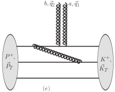
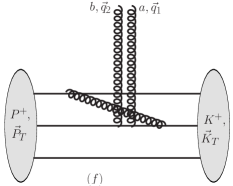
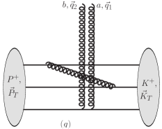
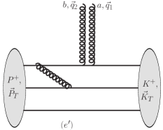
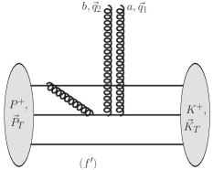
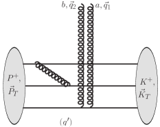
Figure 6: Second set of diagrams for $\langle\rho^{a}_{\mathrm{qu}}(\vec{q}_{1})\,\rho^{b}_{\mathrm{qu}}(\vec{q}_{2})\rangle$. The cut is located at the insertion of the two color charge operators.

The remaining diagrams are finite because the transverse momentum of the gluon shifts the arguments of $\Psi^{*}_{\mathrm{qqq}}$.

$$\mathrm{fig.}\,\ref{fig:rho-rho_qu'}\mathrm{e} = -\frac{g^{4}}{3\cdot 16\pi^{3}}\,C_{F}\,\,\mathrm{tr}\,t^{a}t^{b}\int\left[{\rm d}x_{i}\right]\int\left[{\rm d}^{2}k_{i}\right]\,\Psi_{qqq}(x_{1},\vec{k}_{1};x_{2},\vec{k}_{2};x_{3},\vec{k}_{3})\,$$ (82)

$$\int\limits_{x}^{\mathrm{min}(x_{1},1-x_{2})}\frac{{\rm d}x_{g}}{x_{g}}\left(1-\frac{z_{1}+z_{2}}{2}+\frac{z_{1}z_{2}}{6}\right)\sqrt{\frac{x_{1}}{x_{1}-x_{g}}}\sqrt{\frac{x_{2}}{x_{2}+x_{g}}}$$

$$\int{\rm d}^{2}k_{g}\frac{z_{1}\vec{p}_{1}-\vec{k}_{g}}{\left(z_{1}\vec{p}_{1}-\vec{k}_{g}\right)^{2}}\cdot\frac{z_{2}\vec{p}_{2}-(1-z_{2})\vec{k}_{g}}{\left(z_{2}\vec{p}_{2}-(1-z_{2})\vec{k}_{g}\right)^{2}}$$

$$\Psi_{qqq}^{*}(x_{1}-x_{g},\vec{k}_{1}-(1-x_{1})\vec{q}-\vec{k}_{g}+x_{g}\vec{K};x_{2}+x_{g},\vec{k}_{2}+x_{2}\vec{q}+\vec{k}_{g}-x_{g}\vec{K};x_{3},\vec{k}_{3}+x_{3}\vec{q})~{},$$

with a symmetry factor of 6 (because the gluon may also be absorbed across the insertion by quark 3). The diagram where the gluon is emitted by quark 2 and absorbed by quark 1 is equal to that from fig. 6f and will be included in its symmetry factor.

$$\mathrm{fig.}\,\ref{fig:rho-rho_qu'}\mathrm{f} = -\frac{g^{4}}{3\cdot 16\pi^{3}}\,C_{F}\,\,\mathrm{tr}\,t^{a}t^{b}\int\left[{\rm d}x_{i}\right]\int\left[{\rm d}^{2}k_{i}\right]\,\Psi_{qqq}(x_{1},\vec{k}_{1};x_{2},\vec{k}_{2};x_{3},\vec{k}_{3})\,$$ (83)

$$\int\limits_{x}^{\mathrm{min}(x_{1},1-x_{2})}\frac{{\rm d}x_{g}}{x_{g}}\left(1-\frac{z_{1}+z_{2}}{2}+\frac{z_{1}z_{2}}{6}\right)\sqrt{\frac{x_{1}}{x_{1}-x_{g}}}\sqrt{\frac{x_{2}}{x_{2}+x_{g}}}$$

$$\int{\rm d}^{2}k_{g}\frac{z_{1}\vec{p}_{1}-\vec{k}_{g}}{\left(z_{1}\vec{p}_{1}-\vec{k}_{g}\right)^{2}}\cdot\frac{z_{2}(\vec{p}_{2}-\vec{q})-(1-z_{2})\vec{k}_{g}}{\left(z_{2}(\vec{p}_{2}-\vec{q})-(1-z_{2})\vec{k}_{g}\right)^{2}}$$

$$\Psi_{qqq}^{*}(x_{1}-x_{g},\vec{k}_{1}+x_{1}\vec{q}-\vec{k}_{g}+x_{g}\vec{K};x_{2}+x_{g},\vec{k}_{2}-(1-x_{2})\vec{q}+\vec{k}_{g}-x_{g}\vec{K};x_{3},\vec{k}_{3}+x_{3}\vec{q})~{},$$

again with a symmetry factor of 6.

The diagram where both probes attach to the third quark gives

$$\mathrm{fig.}\,\ref{fig:rho-rho_qu'}\mathrm{g} = -\frac{g^{4}}{3\cdot 16\pi^{3}}\,C_{F}\,\,\mathrm{tr}\,t^{a}t^{b}\int\left[{\rm d}x_{i}\right]\int\left[{\rm d}^{2}k_{i}\right]\,\Psi_{qqq}(x_{1},\vec{k}_{1};x_{2},\vec{k}_{2};x_{3},\vec{k}_{3})\,$$ (84)

$$\int\limits_{x}^{\mathrm{min}(x_{1},1-x_{2})}\frac{{\rm d}x_{g}}{x_{g}}\left(1-\frac{z_{1}+z_{2}}{2}+\frac{z_{1}z_{2}}{6}\right)\sqrt{\frac{x_{1}}{x_{1}-x_{g}}}\sqrt{\frac{x_{2}}{x_{2}+x_{g}}}$$

$$\int{\rm d}^{2}k_{g}\frac{z_{1}\vec{p}_{1}-\vec{k}_{g}}{\left(z_{1}\vec{p}_{1}-\vec{k}_{g}\right)^{2}}\cdot\frac{z_{2}\vec{p}_{2}-(1-z_{2})\vec{k}_{g}}{\left(z_{2}\vec{p}_{2}-(1-z_{2})\vec{k}_{g}\right)^{2}}$$

$$\Psi_{qqq}^{*}(x_{1}-x_{g},\vec{k}_{1}+x_{1}\vec{q}-\vec{k}_{g}+x_{g}\vec{K};x_{2}+x_{g},\vec{k}_{2}+x_{2}\vec{q}+\vec{k}_{g}-x_{g}\vec{K};x_{3},\vec{k}_{3}-(1-x_{3})\vec{q})~{}.$$

Here the symmetry factor is 6 to include the contribution where the gluon emission/absorption vertices are swapped.

Now we list the diagrams where two quarks exchange a gluon on one side of the $\rho^{a}(\vec{q}_{1})\,\rho^{b}(\vec{q}_{2})$ insertion.

$$\mathrm{fig.}\,\ref{fig:rho-rho_qu'}\mathrm{e^{\prime}} = \frac{g^{4}}{3\cdot 16\pi^{3}}\,C_{F}\,\,\mathrm{tr}\,t^{a}t^{b}\int\left[{\rm d}x_{i}\right]\int\left[{\rm d}^{2}k_{i}\right]\,\Psi_{qqq}(x_{1},\vec{k}_{1};x_{2},\vec{k}_{2};x_{3},\vec{k}_{3})\,$$ (85)

$$\int\limits_{x}^{\mathrm{min}(x_{1},1-x_{2})}\frac{{\rm d}x_{g}}{x_{g}}\left(1-\frac{z_{1}+z_{2}}{2}+\frac{z_{1}z_{2}}{6}\right)\sqrt{\frac{x_{1}}{x_{1}-x_{g}}}\sqrt{\frac{x_{2}}{x_{2}+x_{g}}}\int{\rm d}^{2}k_{g}\frac{z_{1}\vec{p}_{1}-\vec{k}_{g}}{\left(z_{1}\vec{p}_{1}-\vec{k}_{g}\right)^{2}}\cdot\frac{z_{2}\vec{p}_{2}-(1-z_{2})\vec{k}_{g}}{\left(z_{2}\vec{p}_{2}-(1-z_{2})\vec{k}_{g}\right)^{2}}$$

$$\Psi_{qqq}^{*}(x_{1}-x_{g},\vec{k}_{1}-(1-x_{1})\vec{q}-\vec{k}_{g}+x_{g}\vec{K};x_{2}+x_{g},\vec{k}_{2}+x_{2}\vec{q}+\vec{k}_{g}-x_{g}\vec{K};x_{3},\vec{k}_{3}+x_{3}\vec{q})~{}.$$

The symmetry factor is $\frac{1}{2}\times 6=3$; the factor of .$\frac{1}{2}$ arises because we sum over all permutations of the gluon exchange within $|P\rangle$.

There is also a diagram (not shown) where quark 2 emits and quark 1 absorbs the gluon on the other side of the insertion:

$$\mathrm{fig.}\,\ref{fig:rho-rho_qu'}\mathrm{e^{\prime\prime}} = \frac{g^{4}}{3\cdot 16\pi^{3}}\,C_{F}\,\,\mathrm{tr}\,t^{a}t^{b}\int\left[{\rm d}x_{i}\right]\int\left[{\rm d}^{2}k_{i}\right]\,\Psi_{qqq}(x_{1},\vec{k}_{1};x_{2},\vec{k}_{2};x_{3},\vec{k}_{3})\,$$ (86)

$$\int\limits_{x}^{\mathrm{min}(x_{1},1-x_{2})}\frac{{\rm d}x_{g}}{x_{g}}\left(1-\frac{z_{1}+z_{2}}{2}+\frac{z_{1}z_{2}}{6}\right)\sqrt{\frac{x_{1}}{x_{1}-x_{g}}}\sqrt{\frac{x_{2}}{x_{2}+x_{g}}}$$

$$\int{\rm d}^{2}k_{g}\frac{z_{1}(\vec{p}_{1}-\vec{q})-\vec{k}_{g}}{\left(z_{1}(\vec{p}_{1}-\vec{q})-\vec{k}_{g}\right)^{2}}\cdot\frac{z_{2}\vec{p}_{2}-(1-z_{2})\vec{k}_{g}}{\left(z_{2}\vec{p}_{2}-(1-z_{2})\vec{k}_{g}\right)^{2}}$$

$$\Psi_{qqq}^{*}(x_{1}-x_{g},\vec{k}_{1}-(1-x_{1})\vec{q}-\vec{k}_{g}+x_{g}\vec{K};x_{2}+x_{g},\vec{k}_{2}+x_{2}\vec{q}+\vec{k}_{g}-x_{g}\vec{K};x_{3},\vec{k}_{3}+x_{3}\vec{q})~{}.$$

Note that here $z_{1}=x_{g}/x_{1}$ and $z_{2}=x_{g}/(x_{2}+x_{g})$, as before. The symmetry factor for this diagram is also 3. Once again, the diagram with swapped emission and absorption vertices is equal to diagram fig. 6f” and will be included in its symmetry factor.

$$\mathrm{fig.}\,\ref{fig:rho-rho_qu'}\mathrm{f^{\prime}} = \frac{g^{4}}{3\cdot 16\pi^{3}}\,C_{F}\,\,\mathrm{tr}\,t^{a}t^{b}\int\left[{\rm d}x_{i}\right]\int\left[{\rm d}^{2}k_{i}\right]\,\Psi_{qqq}(x_{1},\vec{k}_{1};x_{2},\vec{k}_{2};x_{3},\vec{k}_{3})\,$$ (87)

$$\int\limits_{x}^{\mathrm{min}(x_{1},1-x_{2})}\frac{{\rm d}x_{g}}{x_{g}}\left(1-\frac{z_{1}+z_{2}}{2}+\frac{z_{1}z_{2}}{6}\right)\sqrt{\frac{x_{1}}{x_{1}-x_{g}}}\sqrt{\frac{x_{2}}{x_{2}+x_{g}}}\int{\rm d}^{2}k_{g}\frac{z_{1}\vec{p}_{1}-\vec{k}_{g}}{\left(z_{1}\vec{p}_{1}-\vec{k}_{g}\right)^{2}}\cdot\frac{z_{2}\vec{p}_{2}-(1-z_{2})\vec{k}_{g}}{\left(z_{2}\vec{p}_{2}-(1-z_{2})\vec{k}_{g}\right)^{2}}$$

$$\Psi_{qqq}^{*}(x_{1}-x_{g},\vec{k}_{1}+x_{1}\vec{q}-\vec{k}_{g}+x_{g}\vec{K};x_{2}+x_{g},\vec{k}_{2}-(1-x_{2})\vec{q}+\vec{k}_{g}-x_{g}\vec{K};x_{3},\vec{k}_{3}+x_{3}\vec{q})~{}.$$

The symmetry factor is 3.

Again, there is a diagram (not shown) where quark 2 emits and quark 1 absorbs the gluon on the other side of the insertion:

$$\mathrm{fig.}\,\ref{fig:rho-rho_qu'}\mathrm{f^{\prime\prime}} = \frac{g^{4}}{3\cdot 16\pi^{3}}\,C_{F}\,\,\mathrm{tr}\,t^{a}t^{b}\int\left[{\rm d}x_{i}\right]\int\left[{\rm d}^{2}k_{i}\right]\,\Psi_{qqq}(x_{1},\vec{k}_{1};x_{2},\vec{k}_{2};x_{3},\vec{k}_{3})\,$$ (88)

$$\int\limits_{x}^{\mathrm{min}(x_{1},1-x_{2})}\frac{{\rm d}x_{g}}{x_{g}}\left(1-\frac{z_{1}+z_{2}}{2}+\frac{z_{1}z_{2}}{6}\right)\sqrt{\frac{x_{1}}{x_{1}-x_{g}}}\sqrt{\frac{x_{2}}{x_{2}+x_{g}}}$$

$$\int{\rm d}^{2}k_{g}\frac{z_{1}\vec{p}_{1}-\vec{k}_{g}}{\left(z_{1}\vec{p}_{1}-\vec{k}_{g}\right)^{2}}\cdot\frac{z_{2}(\vec{p}_{2}-\vec{q})-(1-z_{2})\vec{k}_{g}}{\left(z_{2}(\vec{p}_{2}-\vec{q})-(1-z_{2})\vec{k}_{g}\right)^{2}}$$

$$\Psi_{qqq}^{*}(x_{1}-x_{g},\vec{k}_{1}+x_{1}\vec{q}-\vec{k}_{g}+x_{g}\vec{K};x_{2}+x_{g},\vec{k}_{2}-(1-x_{2})\vec{q}+\vec{k}_{g}-x_{g}\vec{K};x_{3},\vec{k}_{3}+x_{3}\vec{q})~{}.$$

The symmetry factor is 3.

$$\mathrm{fig.}\,\ref{fig:rho-rho_qu'}\mathrm{g^{\prime}} = \frac{g^{4}}{3\cdot 16\pi^{3}}\,C_{F}\,\,\mathrm{tr}\,t^{a}t^{b}\int\left[{\rm d}x_{i}\right]\int\left[{\rm d}^{2}k_{i}\right]\,\Psi_{qqq}(x_{1},\vec{k}_{1};x_{2},\vec{k}_{2};x_{3},\vec{k}_{3})\,$$ (89)

$$\int\limits_{x}^{\mathrm{min}(x_{1},1-x_{2})}\frac{{\rm d}x_{g}}{x_{g}}\left(1-\frac{z_{1}+z_{2}}{2}+\frac{z_{1}z_{2}}{6}\right)\sqrt{\frac{x_{1}}{x_{1}-x_{g}}}\sqrt{\frac{x_{2}}{x_{2}+x_{g}}}\int{\rm d}^{2}k_{g}\frac{z_{1}\vec{p}_{1}-\vec{k}_{g}}{\left(z_{1}\vec{p}_{1}-\vec{k}_{g}\right)^{2}}\cdot\frac{z_{2}\vec{p}_{2}-(1-z_{2})\vec{k}_{g}}{\left(z_{2}\vec{p}_{2}-(1-z_{2})\vec{k}_{g}\right)^{2}}$$

$$\Psi_{qqq}^{*}(x_{1}-x_{g},\vec{k}_{1}+x_{1}\vec{q}-\vec{k}_{g}+x_{g}\vec{K};x_{2}+x_{g},\vec{k}_{2}+x_{2}\vec{q}+\vec{k}_{g}-x_{g}\vec{K};x_{3},\vec{k}_{3}-(1-x_{3})\vec{q})~{}.$$

The symmetry factor is 3.

$$\mathrm{fig.}\,\ref{fig:rho-rho_qu'}\mathrm{g^{\prime\prime}} = \frac{g^{4}}{3\cdot 16\pi^{3}}\,C_{F}\,\,\mathrm{tr}\,t^{a}t^{b}\int\left[{\rm d}x_{i}\right]\int\left[{\rm d}^{2}k_{i}\right]\,\Psi_{qqq}(x_{1},\vec{k}_{1};x_{2},\vec{k}_{2};x_{3},\vec{k}_{3})\,$$ (90)

$$\int\limits_{x}^{\mathrm{min}(x_{1},1-x_{2})}\frac{{\rm d}x_{g}}{x_{g}}\left(1-\frac{z_{1}+z_{2}}{2}+\frac{z_{1}z_{2}}{6}\right)\sqrt{\frac{x_{1}}{x_{1}-x_{g}}}\sqrt{\frac{x_{2}}{x_{2}+x_{g}}}$$

$$\int{\rm d}^{2}k_{g}\frac{z_{1}\vec{p}_{1}-\vec{k}_{g}}{\left(z_{1}\vec{p}_{1}-\vec{k}_{g}\right)^{2}}\cdot\frac{z_{2}\vec{p}_{2}-(1-z_{2})\vec{k}_{g}}{\left(z_{2}\vec{p}_{2}-(1-z_{2})\vec{k}_{g}\right)^{2}}$$

$$\Psi_{qqq}^{*}(x_{1}-x_{g},\vec{k}_{1}+x_{1}\vec{q}-\vec{k}_{g}+x_{g}\vec{K};x_{2}+x_{g},\vec{k}_{2}+x_{2}\vec{q}+\vec{k}_{g}-x_{g}\vec{K};x_{3},\vec{k}_{3}-(1-x_{3})\vec{q})~{}.$$

The symmetry factor is 3.

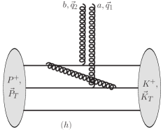
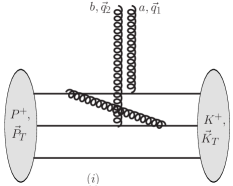
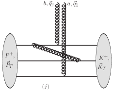
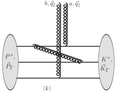
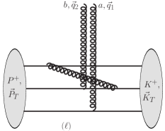
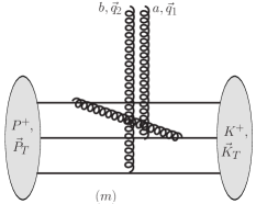
Figure 7: Third set of diagrams for $\langle\rho^{a}_{\mathrm{qu}}(\vec{q}_{1})\,\rho^{b}_{\mathrm{qu}}(\vec{q}_{2})\rangle$.

The third set of diagrams is shown in fig. 7; all their symmetry factors are 6.

$$\mathrm{fig.}\,\ref{fig:rho-rho_qu''}\mathrm{h} = \frac{g^{4}}{3\cdot 16\pi^{3}}\,(\frac{1}{2}-C_{F})\,\,\mathrm{tr}\,t^{a}t^{b}\int\left[{\rm d}x_{i}\right]\int\left[{\rm d}^{2}k_{i}\right]\,\Psi_{qqq}(x_{1},\vec{k}_{1};x_{2},\vec{k}_{2};x_{3},\vec{k}_{3})\,$$ (91)

$$\int\limits_{x}^{\mathrm{min}(x_{1},1-x_{2})}\frac{{\rm d}x_{g}}{x_{g}}\left(1-\frac{z_{1}+z_{2}}{2}+\frac{z_{1}z_{2}}{6}\right)\sqrt{\frac{x_{1}}{x_{1}-x_{g}}}\sqrt{\frac{x_{2}}{x_{2}+x_{g}}}\int{\rm d}^{2}k_{g}\frac{z_{1}\vec{p}_{1}-\vec{k}_{g}}{\left(z_{1}\vec{p}_{1}-\vec{k}_{g}\right)^{2}}\cdot\frac{z_{2}(\vec{p}_{2}-\vec{q}_{1})-(1-z_{2})\vec{k}_{g}}{\left(z_{2}(\vec{p}_{2}-\vec{q}_{1})-(1-z_{2})\vec{k}_{g}\right)^{2}}$$

$$\Psi_{qqq}^{*}(x_{1}-x_{g},\vec{k}_{1}+x_{1}\vec{q}-\vec{q}_{2}-\vec{k}_{g}+x_{g}\vec{K};x_{2}+x_{g},\vec{k}_{2}+x_{2}\vec{q}-\vec{q}_{1}+\vec{k}_{g}-x_{g}\vec{K};x_{3},\vec{k}_{3}+x_{3}\vec{q})~{}.$$

$$\mathrm{fig.}\,\ref{fig:rho-rho_qu''}\mathrm{i} = \mathrm{fig.}\,\ref{fig:rho-rho_qu''}\mathrm{h}\,(\vec{q}_{1}\leftrightarrow\vec{q}_{2})~{}.$$ (92)

$$\mathrm{fig.}\,\ref{fig:rho-rho_qu''}\mathrm{j} = \frac{g^{4}}{3\cdot 16\pi^{3}}\,(C_{F}-\frac{1}{2}-\frac{1}{6})\,\,\mathrm{tr}\,t^{a}t^{b}\int\left[{\rm d}x_{i}\right]\int\left[{\rm d}^{2}k_{i}\right]\,\Psi_{qqq}(x_{1},\vec{k}_{1};x_{2},\vec{k}_{2};x_{3},\vec{k}_{3})\,$$ (93)

$$\int\limits_{x}^{\mathrm{min}(x_{1},1-x_{2})}\frac{{\rm d}x_{g}}{x_{g}}\left(1-\frac{z_{1}+z_{2}}{2}+\frac{z_{1}z_{2}}{6}\right)\sqrt{\frac{x_{1}}{x_{1}-x_{g}}}\sqrt{\frac{x_{2}}{x_{2}+x_{g}}}\int{\rm d}^{2}k_{g}\frac{z_{1}\vec{p}_{1}-\vec{k}_{g}}{\left(z_{1}\vec{p}_{1}-\vec{k}_{g}\right)^{2}}\cdot\frac{z_{2}\vec{p}_{2}-(1-z_{2})\vec{k}_{g}}{\left(z_{2}\vec{p}_{2}-(1-z_{2})\vec{k}_{g}\right)^{2}}$$

$$\Psi_{qqq}^{*}(x_{1}-x_{g},\vec{k}_{1}+x_{1}\vec{q}-\vec{q}_{2}-\vec{k}_{g}+x_{g}\vec{K};x_{2}+x_{g},\vec{k}_{2}+x_{2}\vec{q}+\vec{k}_{g}-x_{g}\vec{K};x_{3},\vec{k}_{3}+x_{3}\vec{q}-\vec{q}_{1})~{}.$$

$$\mathrm{fig.}\,\ref{fig:rho-rho_qu''}\mathrm{k} = \mathrm{fig.}\,\ref{fig:rho-rho_qu''}\mathrm{j}\,(\vec{q}_{1}\leftrightarrow\vec{q}_{2})~{}.$$ (94)

$$\mathrm{fig.}\,\ref{fig:rho-rho_qu''}\ell = \frac{g^{4}}{3\cdot 16\pi^{3}}\,(C_{F}-\frac{1}{2}-\frac{1}{6})\,\,\mathrm{tr}\,t^{a}t^{b}\int\left[{\rm d}x_{i}\right]\int\left[{\rm d}^{2}k_{i}\right]\,\Psi_{qqq}(x_{1},\vec{k}_{1};x_{2},\vec{k}_{2};x_{3},\vec{k}_{3})\,$$ (95)

$$\int\limits_{x}^{\mathrm{min}(x_{1},1-x_{2})}\frac{{\rm d}x_{g}}{x_{g}}\left(1-\frac{z_{1}+z_{2}}{2}+\frac{z_{1}z_{2}}{6}\right)\sqrt{\frac{x_{1}}{x_{1}-x_{g}}}\sqrt{\frac{x_{2}}{x_{2}+x_{g}}}\int{\rm d}^{2}k_{g}\frac{z_{1}\vec{p}_{1}-\vec{k}_{g}}{\left(z_{1}\vec{p}_{1}-\vec{k}_{g}\right)^{2}}\cdot\frac{z_{2}(\vec{p}_{2}-\vec{q}_{2})-(1-z_{2})\vec{k}_{g}}{\left(z_{2}(\vec{p}_{2}-\vec{q}_{2})-(1-z_{2})\vec{k}_{g}\right)^{2}}$$

$$\Psi_{qqq}^{*}(x_{1}-x_{g},\vec{k}_{1}+x_{1}\vec{q}-\vec{k}_{g}+x_{g}\vec{K};x_{2}+x_{g},\vec{k}_{2}+x_{2}\vec{q}-\vec{q}_{2}+\vec{k}_{g}-x_{g}\vec{K};x_{3},\vec{k}_{3}+x_{3}\vec{q}-\vec{q}_{1})~{}.$$

$$\mathrm{fig.}\,\ref{fig:rho-rho_qu''}\mathrm{m} = \mathrm{fig.}\,\ref{fig:rho-rho_qu''}\ell\,(\vec{q}_{1}\leftrightarrow\vec{q}_{2})~{}.$$ (96)

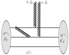
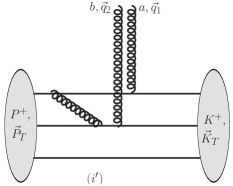
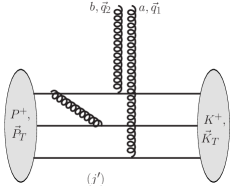
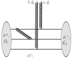
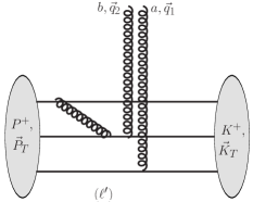
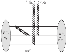
Figure 8: Fourth set of diagrams for $\langle\rho^{a}_{\mathrm{qu}}(\vec{q}_{1})\,\rho^{b}_{\mathrm{qu}}(\vec{q}_{2})\rangle$.

The final set of (finite) diagrams is shown in fig. 8. Here, in $|P\rangle$, quark 1 emits a gluon which is absorbed by quark 2. We will quote with double primes the diagram (not shown) where in $\langle K|$ the exchange occurs from quark 2 to quark 1. All these diagrams have a symmetry factor of $\frac{1}{2}\times 6=3$. As before, in the following expressions $z_{1}=x_{g}/x_{1}$ and $z_{2}=x_{g}/(x_{2}+x_{g})$.

$$\mathrm{fig.}\,\ref{fig:rho-rho_qu'''}\mathrm{h^{\prime}} = -\frac{2g^{4}}{9\cdot 16\pi^{3}}\,\,\mathrm{tr}\,t^{a}t^{b}\int\left[{\rm d}x_{i}\right]\int\left[{\rm d}^{2}k_{i}\right]\,\Psi_{qqq}(x_{1},\vec{k}_{1};x_{2},\vec{k}_{2};x_{3},\vec{k}_{3})\,$$ (97)

$$\int\limits_{x}^{\mathrm{min}(x_{1},1-x_{2})}\frac{{\rm d}x_{g}}{x_{g}}\left(1-\frac{z_{1}+z_{2}}{2}+\frac{z_{1}z_{2}}{6}\right)\sqrt{\frac{x_{1}}{x_{1}-x_{g}}}\sqrt{\frac{x_{2}}{x_{2}+x_{g}}}\int{\rm d}^{2}k_{g}\frac{z_{1}\vec{p}_{1}-\vec{k}_{g}}{\left(z_{1}\vec{p}_{1}-\vec{k}_{g}\right)^{2}}\cdot\frac{z_{2}\vec{p}_{2}-(1-z_{2})\vec{k}_{g}}{\left(z_{2}\vec{p}_{2}-(1-z_{2})\vec{k}_{g}\right)^{2}}$$

$$\Psi_{qqq}^{*}(x_{1}-x_{g},\vec{k}_{1}+x_{1}\vec{q}-\vec{k}_{g}-\vec{q}_{2}+x_{g}\vec{K};x_{2}+x_{g},\vec{k}_{2}+x_{2}\vec{q}+\vec{k}_{g}-\vec{q}_{1}-x_{g}\vec{K};x_{3},\vec{k}_{3}+x_{3}\vec{q})~{}.$$

$$\mathrm{fig.}\,\ref{fig:rho-rho_qu'''}\mathrm{h^{\prime\prime}} = -\frac{2g^{4}}{9\cdot 16\pi^{3}}\,\,\mathrm{tr}\,t^{a}t^{b}\int\left[{\rm d}x_{i}\right]\int\left[{\rm d}^{2}k_{i}\right]\,\Psi_{qqq}(x_{1},\vec{k}_{1};x_{2},\vec{k}_{2};x_{3},\vec{k}_{3})\,$$ (98)

$$\int\limits_{x}^{\mathrm{min}(x_{1},1-x_{2})}\frac{{\rm d}x_{g}}{x_{g}}\left(1-\frac{z_{1}+z_{2}}{2}+\frac{z_{1}z_{2}}{6}\right)\sqrt{\frac{x_{1}}{x_{1}-x_{g}}}\sqrt{\frac{x_{2}}{x_{2}+x_{g}}}\int{\rm d}^{2}k_{g}\frac{z_{1}(\vec{p}_{1}-\vec{q}_{2})-\vec{k}_{g}}{\left(z_{1}(\vec{p}_{1}-\vec{q}_{2})-\vec{k}_{g}\right)^{2}}\cdot\frac{z_{2}(\vec{p}_{2}-\vec{q}_{1})-(1-z_{2})\vec{k}_{g}}{\left(z_{2}(\vec{p}_{2}-\vec{q}_{1})-(1-z_{2})\vec{k}_{g}\right)^{2}}$$

$$\Psi_{qqq}^{*}(x_{1}-x_{g},\vec{k}_{1}+x_{1}\vec{q}-\vec{k}_{g}-\vec{q}_{2}+x_{g}\vec{K};x_{2}+x_{g},\vec{k}_{2}+x_{2}\vec{q}+\vec{k}_{g}-\vec{q}_{1}-x_{g}\vec{K};x_{3},\vec{k}_{3}+x_{3}\vec{q})~{}.$$

$$\mathrm{fig.}\,\ref{fig:rho-rho_qu'''}\mathrm{i^{\prime}} = \mathrm{fig.}\,\ref{fig:rho-rho_qu'''}\mathrm{h^{\prime}}(\vec{q}_{1}\leftrightarrow\vec{q}_{2})~{}.$$ (99)

$$\mathrm{fig.}\,\ref{fig:rho-rho_qu'''}\mathrm{i^{\prime\prime}} = \mathrm{fig.}\,\ref{fig:rho-rho_qu'''}\mathrm{h^{\prime\prime}}(\vec{q}_{1}\leftrightarrow\vec{q}_{2})~{}.$$ (100)

$$\mathrm{fig.}\,\ref{fig:rho-rho_qu'''}\mathrm{j^{\prime}} = -\frac{g^{4}}{3\cdot 16\pi^{3}}\,(C_{F}-\frac{2}{3})\,\,\mathrm{tr}\,t^{a}t^{b}\int\left[{\rm d}x_{i}\right]\int\left[{\rm d}^{2}k_{i}\right]\,\Psi_{qqq}(x_{1},\vec{k}_{1};x_{2},\vec{k}_{2};x_{3},\vec{k}_{3})\,$$ (101)

$$\int\limits_{x}^{\mathrm{min}(x_{1},1-x_{2})}\frac{{\rm d}x_{g}}{x_{g}}\left(1-\frac{z_{1}+z_{2}}{2}+\frac{z_{1}z_{2}}{6}\right)\sqrt{\frac{x_{1}}{x_{1}-x_{g}}}\sqrt{\frac{x_{2}}{x_{2}+x_{g}}}\int{\rm d}^{2}k_{g}\frac{z_{1}\vec{p}_{1}-\vec{k}_{g}}{\left(z_{1}\vec{p}_{1}-\vec{k}_{g}\right)^{2}}\cdot\frac{z_{2}\vec{p}_{2}-(1-z_{2})\vec{k}_{g}}{\left(z_{2}\vec{p}_{2}-(1-z_{2})\vec{k}_{g}\right)^{2}}$$

$$\Psi_{qqq}^{*}(x_{1}-x_{g},\vec{k}_{1}+x_{1}\vec{q}-\vec{k}_{g}-\vec{q}_{2}+x_{g}\vec{K};x_{2}+x_{g},\vec{k}_{2}+x_{2}\vec{q}+\vec{k}_{g}-x_{g}\vec{K};x_{3},\vec{k}_{3}+x_{3}\vec{q}-\vec{q}_{1})~{}.$$

$$\mathrm{fig.}\,\ref{fig:rho-rho_qu'''}\mathrm{j^{\prime\prime}} = -\frac{g^{4}}{3\cdot 16\pi^{3}}\,(C_{F}-\frac{2}{3})\,\,\mathrm{tr}\,t^{a}t^{b}\int\left[{\rm d}x_{i}\right]\int\left[{\rm d}^{2}k_{i}\right]\,\Psi_{qqq}(x_{1},\vec{k}_{1};x_{2},\vec{k}_{2};x_{3},\vec{k}_{3})\,$$ (102)

$$\int\limits_{x}^{\mathrm{min}(x_{1},1-x_{2})}\frac{{\rm d}x_{g}}{x_{g}}\left(1-\frac{z_{1}+z_{2}}{2}+\frac{z_{1}z_{2}}{6}\right)\sqrt{\frac{x_{1}}{x_{1}-x_{g}}}\sqrt{\frac{x_{2}}{x_{2}+x_{g}}}\int{\rm d}^{2}k_{g}\frac{z_{1}(\vec{p}_{1}-\vec{q}_{2})-\vec{k}_{g}}{\left(z_{1}(\vec{p}_{1}-\vec{q}_{2})-\vec{k}_{g}\right)^{2}}\cdot\frac{z_{2}\vec{p}_{2}-(1-z_{2})\vec{k}_{g}}{\left(z_{2}\vec{p}_{2}-(1-z_{2})\vec{k}_{g}\right)^{2}}$$

$$\Psi_{qqq}^{*}(x_{1}-x_{g},\vec{k}_{1}+x_{1}\vec{q}-\vec{k}_{g}-\vec{q}_{2}+x_{g}\vec{K};x_{2}+x_{g},\vec{k}_{2}+x_{2}\vec{q}+\vec{k}_{g}-x_{g}\vec{K};x_{3},\vec{k}_{3}+x_{3}\vec{q}-\vec{q}_{1})~{}.$$

$$\mathrm{fig.}\,\ref{fig:rho-rho_qu'''}\mathrm{k^{\prime}} = \mathrm{fig.}\,\ref{fig:rho-rho_qu'''}\mathrm{j^{\prime}}(\vec{q}_{1}\leftrightarrow\vec{q}_{2})~{}.$$ (103)

$$\mathrm{fig.}\,\ref{fig:rho-rho_qu'''}\mathrm{k^{\prime\prime}} = \mathrm{fig.}\,\ref{fig:rho-rho_qu'''}\mathrm{j^{\prime\prime}}(\vec{q}_{1}\leftrightarrow\vec{q}_{2})~{}.$$ (104)

$$\mathrm{fig.}\,\ref{fig:rho-rho_qu'''}\mathrm{\ell^{\prime}} = -\frac{g^{4}}{3\cdot 16\pi^{3}}\,(C_{F}-\frac{2}{3})\,\,\mathrm{tr}\,t^{a}t^{b}\int\left[{\rm d}x_{i}\right]\int\left[{\rm d}^{2}k_{i}\right]\,\Psi_{qqq}(x_{1},\vec{k}_{1};x_{2},\vec{k}_{2};x_{3},\vec{k}_{3})\,$$ (105)

$$\int\limits_{x}^{\mathrm{min}(x_{1},1-x_{2})}\frac{{\rm d}x_{g}}{x_{g}}\left(1-\frac{z_{1}+z_{2}}{2}+\frac{z_{1}z_{2}}{6}\right)\sqrt{\frac{x_{1}}{x_{1}-x_{g}}}\sqrt{\frac{x_{2}}{x_{2}+x_{g}}}\int{\rm d}^{2}k_{g}\frac{z_{1}\vec{p}_{1}-\vec{k}_{g}}{\left(z_{1}\vec{p}_{1}-\vec{k}_{g}\right)^{2}}\cdot\frac{z_{2}\vec{p}_{2}-(1-z_{2})\vec{k}_{g}}{\left(z_{2}\vec{p}_{2}-(1-z_{2})\vec{k}_{g}\right)^{2}}$$

$$\Psi_{qqq}^{*}(x_{1}-x_{g},\vec{k}_{1}+x_{1}\vec{q}-\vec{k}_{g}+x_{g}\vec{K};x_{2}+x_{g},\vec{k}_{2}+x_{2}\vec{q}+\vec{k}_{g}-\vec{q}_{2}-x_{g}\vec{K};x_{3},\vec{k}_{3}+x_{3}\vec{q}-\vec{q}_{1})~{}.$$

$$\mathrm{fig.}\,\ref{fig:rho-rho_qu'''}\mathrm{\ell^{\prime\prime}} = -\frac{g^{4}}{3\cdot 16\pi^{3}}\,(C_{F}-\frac{2}{3})\,\,\mathrm{tr}\,t^{a}t^{b}\int\left[{\rm d}x_{i}\right]\int\left[{\rm d}^{2}k_{i}\right]\,\Psi_{qqq}(x_{1},\vec{k}_{1};x_{2},\vec{k}_{2};x_{3},\vec{k}_{3})\,$$ (106)

$$\int\limits_{x}^{\mathrm{min}(x_{1},1-x_{2})}\frac{{\rm d}x_{g}}{x_{g}}\left(1-\frac{z_{1}+z_{2}}{2}+\frac{z_{1}z_{2}}{6}\right)\sqrt{\frac{x_{1}}{x_{1}-x_{g}}}\sqrt{\frac{x_{2}}{x_{2}+x_{g}}}\int{\rm d}^{2}k_{g}\frac{z_{1}\vec{p}_{1}-\vec{k}_{g}}{\left(z_{1}\vec{p}_{1}-\vec{k}_{g}\right)^{2}}\cdot\frac{z_{2}(\vec{p}_{2}-\vec{q}_{2})-(1-z_{2})\vec{k}_{g}}{\left(z_{2}(\vec{p}_{2}-\vec{q}_{2})-(1-z_{2})\vec{k}_{g}\right)^{2}}$$

$$\Psi_{qqq}^{*}(x_{1}-x_{g},\vec{k}_{1}+x_{1}\vec{q}-\vec{k}_{g}+x_{g}\vec{K};x_{2}+x_{g},\vec{k}_{2}+x_{2}\vec{q}+\vec{k}_{g}-\vec{q}_{2}-x_{g}\vec{K};x_{3},\vec{k}_{3}+x_{3}\vec{q}-\vec{q}_{1})~{}.$$

$$\mathrm{fig.}\,\ref{fig:rho-rho_qu'''}\mathrm{m^{\prime}} = \mathrm{fig.}\,\ref{fig:rho-rho_qu'''}\mathrm{\ell^{\prime}}(\vec{q}_{1}\leftrightarrow\vec{q}_{2})~{}.$$ (107)

$$\mathrm{fig.}\,\ref{fig:rho-rho_qu'''}\mathrm{m^{\prime\prime}} = \mathrm{fig.}\,\ref{fig:rho-rho_qu'''}\mathrm{\ell^{\prime\prime}}(\vec{q}_{1}\leftrightarrow\vec{q}_{2})~{}.$$ (108)

IV.3 Cancellation of UV divergences

In this section we collect all UV divergent diagrams to verify that the divergent contributions to $\langle\rho^{a}(\vec{q}_{1})\,\rho^{b}(\vec{q}_{2})\rangle$ cancel, to leave just the finite parts. This implies that at this order $\langle\rho^{a}(\vec{q}_{1})\,\rho^{b}(\vec{q}_{2})\rangle$ is independent of the renormalization scale.

We consider the diagrams where quark 1 exchanges a gluon with itself.

We begin with the diagrams where the charge operators couple to either the gluon or quark 1. The UV divergent contribution of all these diagrams is proportional to

$$2\pi^{3}\frac{g^{2}}{3\cdot 16\pi^{3}}\,\delta^{ab}\int\left[{\rm d}x_{i}\right]\int\left[{\rm d}^{2}k_{i}\right]\,C_{q}(x_{1})\,\Psi_{qqq}(x_{1},\vec{k}_{1};x_{2},\vec{k}_{2};x_{3},\vec{k}_{3})\,$$

$$~{}~{}~{}~{}~{}~{}\Psi_{qqq}^{*}(x_{1},\vec{k}_{1}-(1-x_{1})\vec{q};x_{2},\vec{k}_{2}+x_{2}\vec{q};x_{3},\vec{k}_{3}+x_{3}\vec{q})~{}.$$ (109)

We now collect all the prefactors. Fig. 2a comes with a factor of $2\cdot 3/C_{F}$ while fig. 3a, plus the corresponding diagram for $\vec{q}_{1}\leftrightarrow\vec{q}_{2}$, contributes $-2\cdot 3/C_{F}$.

From fig. 4a, plus the corresponding diagram where the gluon emission and reabsorption occurs on the other side of the insertion, we get $-\frac{1}{6}\cdot\frac{1}{2}\cdot 3\cdot 16\pi^{3}/2\pi^{3}=-2$. On the other hand, fig. 5a contributes $4\cdot\frac{1}{2}$.

Next is the contribution where both probes couple to the second quark. From the diagram analogous to fig. 4a, with both probes attached to quark 2, we again get $-\frac{1}{6}\cdot\frac{1}{2}\cdot 3\cdot 16\pi^{3}/2\pi^{3}=-2$. Fig. 5b contributes $4\cdot\frac{1}{2}=2$.

Now consider the diagrams where the first probe ($a,\vec{q}_{1}$) attaches to quark 2 while the second probe ($b,\vec{q}_{2}$) attaches either to quark 1 or to the gluon in the proton. Fig. 3b comes with a prefactor of $-\frac{1}{2}\cdot 3/C_{F}=-9/8$. The prefactor of fig. 5c is $\frac{2}{6}\cdot\frac{1}{2}/C_{F}=1/8$. Lastly, from the third term in eq. (76), which is a diagram like fig. 4a but with the first probe attached to quark 2, we get $\frac{1}{6}\cdot\frac{1}{2}\cdot\frac{1}{2}\cdot 3\cdot 16\pi^{3}/2\pi^{3}=1$.

Finally, we turn to the diagrams where the first probe ($a,\vec{q}_{1}$) attaches to quark 3 while the second probe ($b,\vec{q}_{2}$) attaches to quark 2. The contribution from diagrams of the type of fig. 4 where quark 1 exchanges a gluon with itself on either side of the insertion (second term in eq. (76) with quarks 1 and 3 interchanged, multiplied by $-C_{q}(x_{1})$) we get $\frac{1}{6}\cdot\frac{1}{2}\cdot\frac{1}{2}\cdot 3\cdot 16\pi^{3}/2\pi^{3}=1$. Fig. 5d contributes $-2\cdot\frac{1}{2}$.

IV.4 Decoupling of gluon probes with infinite transverse wave length

Here we verify that $\langle\rho^{a}(\vec{q}_{1})\,\rho^{b}(\vec{q}_{2})\rangle$ vanishes when either one of the transverse momenta goes to zero; we consider $\vec{q}_{1}\to 0$, the other case follows by symmetry. In intuitive terms this reflects the fact that a gluon with infinite wave length does not couple to a color singlet proton.

Since we have already verified in the previous section that all UV divergences cancel we may now discard the divergent pieces of all diagrams and focus on their finite parts.

The charge correlator at ${\cal O}(g^{2})$ given in eq. (76) does indeed vanish when $\vec{q}_{1}\to 0$, on account of the symmetry of the three quark wave function $\Psi_{\mathrm{qqq}}$ under exchange of any two quarks. For the rest of this section we consider the contributions to $\langle\rho^{a}(\vec{q}_{1})\,\rho^{b}(\vec{q}_{2})\rangle$ at ${\cal O}(g^{4})$.

For the purpose of more compact expressions we will split off the “pre-factor”

$$3\frac{g^{4}}{16\pi^{3}}\,\delta^{ab}\,\int[{\rm d}x_{i}]\int[{\rm d}^{2}k_{i}]\Psi_{qqq}(x_{1},\vec{k}_{1};x_{2},\vec{k}_{2};x_{3},\vec{k}_{3})~{},$$ (110)

which includes a symmetry factor of 3, from the following expressions.

We collect first all the terms from the divergent diagrams which involve $\Psi_{qqq}^{*}(x_{1},\vec{k}_{1}-(1-x_{1})\vec{q}_{2};x_{2},\vec{k}_{2}+x_{2}\vec{q}_{2};x_{3},\vec{k}_{3}+x_{3}\vec{q}_{2})$: eq. (65), eq. (70) plus $\vec{q}_{1}\leftrightarrow\vec{q}_{2}$, two times eq. (71) plus $\vec{q}_{1}\leftrightarrow\vec{q}_{2}$ (with quarks 1 and 2 interchanged), eq. (77), eq. (78), eq. (79) plus $\vec{q}_{1}\leftrightarrow\vec{q}_{2}$ (with quarks 1 and 2 interchanged), and eq. (81) (with quarks 1 and 2 interchanged):

$$\begin{split}&2\cdot 2\pi^{3}F(\vec{q}_{2},0,\frac{x}{x_{1}},m^{2})\\ -&2\pi^{3}F(\vec{q}_{2},0,\frac{x}{x_{1}},m^{2})\\ -&2\pi^{3}F(\vec{q}_{2},\vec{q}_{2},\frac{x}{x_{1}},m^{2})\\ -&2\cdot\frac{1}{2}\cdot 2\pi^{3}F(\vec{q}_{2},0,\frac{x}{x_{1}},m^{2})\\ -&2\cdot\frac{1}{2}\cdot 2\pi^{3}F(0,0,\frac{x}{x_{2}},m^{2})\\ +&\frac{4}{3}\cdot C_{F}\cdot\frac{1}{2}\cdot 2\pi^{3}F(\vec{q}_{2},\vec{q}_{2},\frac{x}{x_{1}},m^{2})\\ +&2\cdot\frac{4}{3}\cdot C_{F}\cdot\frac{1}{2}\cdot 2\pi^{3}F(0,0,\frac{x}{x_{2}},m^{2})\\ +&2\cdot\frac{2}{18}\cdot\frac{1}{2}\cdot 2\pi^{3}F(\vec{q}_{2},\vec{q}_{2},\frac{x}{x_{1}},m^{2})\\ +&2\cdot\frac{2}{18}\cdot\frac{1}{2}\cdot 2\pi^{3}F(0,0,\frac{x}{x_{2}},m^{2})\\ -&2\cdot\frac{2}{3}\cdot C_{F}\cdot\frac{1}{2}\cdot 2\pi^{3}F(0,0,\frac{x}{x_{2}},m^{2})\\ =&~{}0~{}.\end{split}$$ (111)

The remaining terms which involve $\Psi_{qqq}^{*}(x_{1}-x_{g},\vec{k}_{1}-(1-x_{1})\vec{q}_{2}-\vec{k}_{g}+x_{g}\vec{K};x_{2}+x_{g},\vec{k}_{2}+x_{2}\vec{q}_{2}+\vec{k}_{g}-x_{g}\vec{K};x_{3},\vec{k}_{3}+x_{3}\vec{q}_{2})$, again with the “pre-factor” (114): eq. (72) with $\vec{q}_{1}\leftrightarrow\vec{q}_{2}$, eq. (82, 85, 91, 93, 97, 101),

$$\begin{split}&2\cdot\frac{1}{12}\cdot 3\cdot\frac{z_{2}\vec{p}_{2}-(1-z_{2})\vec{k}_{g}}{\left(z_{2}\vec{p}_{2}-(1-z_{2})\vec{k}_{g}\right)^{2}}\\ -&2\cdot\frac{1}{3}\cdot C_{F}\cdot\frac{1}{2}\cdot\frac{z_{2}\vec{p}_{2}-(1-z_{2})\vec{k}_{g}}{\left(z_{2}\vec{p}_{2}-(1-z_{2})\vec{k}_{g}\right)^{2}}\\ +&\frac{1}{3}\cdot C_{F}\cdot\frac{1}{2}\cdot\frac{z_{2}\vec{p}_{2}-(1-z_{2})\vec{k}_{g}}{\left(z_{2}\vec{p}_{2}-(1-z_{2})\vec{k}_{g}\right)^{2}}\\ +&2\cdot\frac{1}{3}\cdot(\frac{1}{2}-C_{F})\cdot\frac{1}{2}\cdot\frac{z_{2}\vec{p}_{2}-(1-z_{2})\vec{k}_{g}}{\left(z_{2}\vec{p}_{2}-(1-z_{2})\vec{k}_{g}\right)^{2}}\\ +&2\cdot\frac{1}{3}\cdot(C_{F}-\frac{2}{3})\cdot\frac{1}{2}\cdot\frac{z_{2}\vec{p}_{2}-(1-z_{2})\vec{k}_{g}}{\left(z_{2}\vec{p}_{2}-(1-z_{2})\vec{k}_{g}\right)^{2}}\\ -&\frac{2}{9}\cdot\frac{1}{2}\cdot\frac{z_{2}\vec{p}_{2}-(1-z_{2})\vec{k}_{g}}{\left(z_{2}\vec{p}_{2}-(1-z_{2})\vec{k}_{g}\right)^{2}}\\ -&\frac{1}{3}\cdot(C_{F}-\frac{2}{3})\cdot\frac{1}{2}\cdot\frac{z_{2}\vec{p}_{2}-(1-z_{2})\vec{k}_{g}}{\left(z_{2}\vec{p}_{2}-(1-z_{2})\vec{k}_{g}\right)^{2}}\\ &=0~{}.\end{split}$$ (112)

There are three more contributions which involve $\Psi_{qqq}^{*}(x_{1}-x_{g},\vec{k}_{1}-(1-x_{1})\vec{q}_{2}-\vec{k}_{g}+x_{g}\vec{K};x_{2}+x_{g},\vec{k}_{2}+x_{2}\vec{q}_{2}+\vec{k}_{g}-x_{g}\vec{K};x_{3},\vec{k}_{3}+x_{3}\vec{q}_{2})$ but the structure

$$\frac{z_{1}(\vec{p}_{1}-\vec{q}_{2})-\vec{k}_{g}}{(z_{1}(\vec{p}_{1}-\vec{q}_{2})-\vec{k}_{g})^{2}}\cdot\frac{z_{2}\vec{p}_{2}-(1-z_{2})\vec{k}_{g}}{(z_{2}\vec{p}_{2}-(1-z_{2})\vec{k}_{g})^{2}}~{}.$$ (113)

These are eq. (86) with a prefactor of $2/9$, and eqs. (98, 102) each with a prefactor of $-1/9$.

Next, we collect terms which involve $\Psi_{qqq}^{*}(x_{1}-x_{g},\vec{k}_{1}+x_{1}\vec{q}_{2}-\vec{k}_{g}+x_{g}\vec{K};x_{2}+x_{g},\vec{k}_{2}-(1-x_{2})\vec{q}_{2}+\vec{k}_{g}-x_{g}\vec{K};x_{3},\vec{k}_{3}+x_{3}\vec{q}_{2})$. Here, we split off the “pre-factor”

$$\begin{split}&3\frac{g^{4}}{16\pi^{3}}\,\delta^{ab}\int\left[{\rm d}x_{i}\right]\int\left[{\rm d}^{2}k_{i}\right]\,\Psi_{qqq}(x_{1},\vec{k}_{1};x_{2},\vec{k}_{2};x_{3},\vec{k}_{3})\,\int\limits_{x}^{\mathrm{min}(x_{1},1-x_{2})}\frac{{\rm d}x_{g}}{x_{g}}\\ &\int{\rm d}^{2}k_{g}\sqrt{\frac{x_{1}}{x_{1}-x_{g}}}\sqrt{\frac{x_{2}}{x_{2}+x_{g}}}\left(1-\frac{z_{1}+z_{2}}{2}+\frac{z_{1}z_{2}}{6}\right)\frac{z_{1}\vec{p}_{1}-\vec{k}_{g}}{\left(z_{1}\vec{p}_{1}-\vec{k}_{g}\right)^{2}}\cdot~{},\end{split}$$ (114)

which includes a factor of 3 out of the symmetry factors of the diagrams. These are: eqs. (68, 72), eq. (73) plus $\vec{q}_{1}\leftrightarrow\vec{q}_{2}$, eq. (83, 87, 88, 92, 95, 99, 100, 105, 106)

$$\begin{split}-&2\cdot\frac{1}{6}\cdot 3\cdot\frac{z_{2}\vec{p}_{2}-(1-z_{2})(\vec{k}_{g}-\vec{q}_{2})}{\left(z_{2}\vec{p}_{2}-(1-z_{2})(\vec{k}_{g}-\vec{q}_{2})\right)^{2}}\\ +&2\cdot\frac{1}{12}\cdot 3\cdot\frac{z_{2}\vec{p}_{2}-(1-z_{2})(\vec{k}_{g}-\vec{q}_{2})}{\left(z_{2}\vec{p}_{2}-(1-z_{2})(\vec{k}_{g}-\vec{q}_{2})\right)^{2}}\\ +&2\cdot\frac{1}{12}\cdot 3\cdot\frac{z_{2}\vec{p}_{2}-(1-z_{2})(\vec{k}_{g}-\vec{q}_{2})}{\left(z_{2}\vec{p}_{2}-(1-z_{2})(\vec{k}_{g}-\vec{q}_{2})\right)^{2}}\\ +&2\cdot\frac{1}{12}\cdot 3\cdot\frac{z_{2}(\vec{p}_{2}-\vec{q}_{2})-(1-z_{2})\vec{k}_{g}}{\left(z_{2}(\vec{p}_{2}-\vec{q}_{2})-(1-z_{2})\vec{k}_{g}\right)^{2}}\\ -&2\cdot\frac{1}{3}\cdot C_{F}\cdot\frac{1}{2}\cdot\frac{z_{2}(\vec{p}_{2}-\vec{q}_{2})-(1-z_{2})\vec{k}_{g}}{\left(z_{2}(\vec{p}_{2}-\vec{q}_{2})-(1-z_{2})\vec{k}_{g}\right)^{2}}\\ +&\frac{1}{3}\cdot C_{F}\cdot\frac{1}{2}\cdot\frac{z_{2}\vec{p}_{2}-(1-z_{2})\vec{k}_{g}}{\left(z_{2}\vec{p}_{2}-(1-z_{2})\vec{k}_{g}\right)^{2}}\\ +&\frac{1}{3}\cdot C_{F}\cdot\frac{1}{2}\cdot\frac{z_{2}(\vec{p}_{2}-\vec{q}_{2})-(1-z_{2})\vec{k}_{g}}{\left(z_{2}(\vec{p}_{2}-\vec{q}_{2})-(1-z_{2})\vec{k}_{g}\right)^{2}}\\ +&2\cdot\frac{1}{3}(\frac{1}{2}-C_{F})\cdot\frac{1}{2}\cdot\frac{z_{2}(\vec{p}_{2}-\vec{q}_{2})-(1-z_{2})\vec{k}_{g}}{\left(z_{2}(\vec{p}_{2}-\vec{q}_{2})-(1-z_{2})\vec{k}_{g}\right)^{2}}\\ -&2\cdot\frac{1}{3}(\frac{2}{3}-C_{F})\cdot\frac{1}{2}\cdot\frac{z_{2}(\vec{p}_{2}-\vec{q}_{2})-(1-z_{2})\vec{k}_{g}}{\left(z_{2}(\vec{p}_{2}-\vec{q}_{2})-(1-z_{2})\vec{k}_{g}\right)^{2}}\\ -&\frac{2}{9}\cdot\frac{1}{2}\cdot\frac{z_{2}\vec{p}_{2}-(1-z_{2})\vec{k}_{g}}{\left(z_{2}\vec{p}_{2}-(1-z_{2})\vec{k}_{g}\right)^{2}}\\ -&\frac{2}{9}\cdot\frac{1}{2}\cdot\frac{z_{2}(\vec{p}_{2}-\vec{q}_{2})-(1-z_{2})\vec{k}_{g}}{\left(z_{2}(\vec{p}_{2}-\vec{q}_{2})-(1-z_{2})\vec{k}_{g}\right)^{2}}\\ -&\frac{1}{3}\cdot(C_{F}-\frac{2}{3})\cdot\frac{1}{2}\cdot\frac{z_{2}\vec{p}_{2}-(1-z_{2})\vec{k}_{g}}{\left(z_{2}\vec{p}_{2}-(1-z_{2})\vec{k}_{g}\right)^{2}}\\ -&\frac{1}{3}\cdot(C_{F}-\frac{2}{3})\cdot\frac{1}{2}\cdot\frac{z_{2}(\vec{p}_{2}-\vec{q}_{2})-(1-z_{2})\vec{k}_{g}}{\left(z_{2}(\vec{p}_{2}-\vec{q}_{2})-(1-z_{2})\vec{k}_{g}\right)^{2}}\\ &=0~{}.\end{split}$$ (115)

Lastly, we collect terms which involve $\Psi_{qqq}^{*}(x_{1}-x_{g},\vec{k}_{1}+x_{1}\vec{q}_{2}-\vec{k}_{g}+x_{g}\vec{K};x_{2}+x_{g},\vec{k}_{2}+x_{2}\vec{q}_{2}+\vec{k}_{g}-x_{g}\vec{K};x_{3},\vec{k}_{3}-(1-x_{3})\vec{q}_{2})$, with the “pre-factor” (114): eq. (84, 89, 90, 94, 96, 103, 104, 107, 108),

$$- 2\cdot\frac{C_{F}}{3}\cdot\frac{1}{2}\cdot\frac{z_{2}\vec{p}_{2}-(1-z_{2})\vec{k}_{g}}{\left(z_{2}\vec{p}_{2}-(1-z_{2})\vec{k}_{g}\right)^{2}}$$ (116)

$$+ \frac{C_{F}}{3}\cdot\frac{1}{2}\cdot\frac{z_{2}\vec{p}_{2}-(1-z_{2})\vec{k}_{g}}{\left(z_{2}\vec{p}_{2}-(1-z_{2})\vec{k}_{g}\right)^{2}}$$

$$+ \frac{C_{F}}{3}\cdot\frac{1}{2}\cdot\frac{z_{2}\vec{p}_{2}-(1-z_{2})\vec{k}_{g}}{\left(z_{2}\vec{p}_{2}-(1-z_{2})\vec{k}_{g}\right)^{2}}$$

$$+ 2\cdot\frac{1}{3}\cdot(C_{F}-\frac{2}{3})\cdot\frac{1}{2}\cdot\frac{z_{2}\vec{p}_{2}-(1-z_{2})\vec{k}_{g}}{\left(z_{2}\vec{p}_{2}-(1-z_{2})\vec{k}_{g}\right)^{2}}$$

$$+ 2\cdot\frac{1}{3}\cdot(C_{F}-\frac{2}{3})\cdot\frac{1}{2}\cdot\frac{z_{2}\vec{p}_{2}-(1-z_{2})\vec{k}_{g}}{\left(z_{2}\vec{p}_{2}-(1-z_{2})\vec{k}_{g}\right)^{2}}$$

$$- \frac{1}{3}\cdot(C_{F}-\frac{2}{3})\cdot\frac{1}{2}\cdot\frac{z_{2}\vec{p}_{2}-(1-z_{2})\vec{k}_{g}}{\left(z_{2}\vec{p}_{2}-(1-z_{2})\vec{k}_{g}\right)^{2}}$$

$$- \frac{1}{3}\cdot(C_{F}-\frac{2}{3})\cdot\frac{1}{2}\cdot\frac{z_{2}\vec{p}_{2}-(1-z_{2})\vec{k}_{g}}{\left(z_{2}\vec{p}_{2}-(1-z_{2})\vec{k}_{g}\right)^{2}}$$

$$- \frac{1}{3}\cdot(C_{F}-\frac{2}{3})\cdot\frac{1}{2}\cdot\frac{z_{2}\vec{p}_{2}-(1-z_{2})\vec{k}_{g}}{\left(z_{2}\vec{p}_{2}-(1-z_{2})\vec{k}_{g}\right)^{2}}$$

$$- \frac{1}{3}\cdot(C_{F}-\frac{2}{3})\cdot\frac{1}{2}\cdot\frac{z_{2}\vec{p}_{2}-(1-z_{2})\vec{k}_{g}}{\left(z_{2}\vec{p}_{2}-(1-z_{2})\vec{k}_{g}\right)^{2}}$$

$$=0~{}.$$

V Outlook

Ref. Dumitru et al. (2020) showed “sub-femtometer” scale color charge correlations in a proton composed of three quarks. These correlators were found to display interesting dependence on the impact parameter and on the relative momentum of the gluon probes, rather than being simply proportional to the one-body particle density in the proton.

Here, we have computed the expressions for the $\langle\rho^{a}(\vec{q}_{1})\,\rho^{b}(\vec{q}_{2})\rangle$ correlator in a proton made of three quarks and a perturbative gluon (which is not required to carry a small light-cone momentum). These results may be used to obtain a more realistic picture of color charge correlations in the proton at moderate $x\,\,\vbox{\hbox{$\buildrel\displaystyle>\over{\sim}$}}\,\,0.01$. Also, they could be used to “jump-start” small-$x$ BK evolution, in particular impact parameter dependent evolution Golec-Biernat and Stasto (2003); Berger and Stasto (2011); Cepila et al. (2019); Bendova et al. (2019), towards $x\ll 0.01$ from a better constrained and perhaps more realistic initial condition.

It would be very interesting to obtain numerical results for the color charge correlator as a function of impact parameter $\vec{b}$ and relative transverse position $\vec{r}$ of the probes. For numerical estimates one could employ a model for the non-perturbative valence quark wave function such as the one of ref. Schlumpf (1993); Brodsky and Schlumpf (1994); it encodes the proper proton radius and average quark longitudinal and transverse momentum, as well as momentum correlations among the valence quarks.

Furthermore, the present calculation should be extended to the correlator of three charge operators, $\langle\rho^{a}(\vec{q}_{1})\,\rho^{b}(\vec{q}_{2})\,\rho^{c}(\vec{q}_{3})\rangle$; the contribution of the $|qqq\rangle$ Fock state has been analyzed in ref. Dumitru et al. (2020). $C$-odd three-gluon exchange gives an imaginary contribution to the dipole scattering amplitude [or a real part, respectively, if ${\cal T}\to i{\cal T}$ in eq. (2)]. It is related to various spin dependent Transverse Momentum Dependent (TMD) distributions such as the (dipole) gluon Sivers function of a transversely polarized proton Yao et al. (2019). This amplitude is also relevant for charge asymmetries in diffractive electroproduction of a $\pi^{+}\,\pi^{-}$ pair Hägler et al. (2002); Hagler et al. (2002) or for exclusive production of a pseudo-scalar meson Dumitru and Stebel (2019); Czyzewski et al. (1997); Engel et al. (1998); Kilian and Nachtmann (1998). Work is in progress to account for corrections to the three-gluon exchange amplitude due to a perturbative gluon in the proton, and will be reported elsewhere.

Appendix A Regularization of the integral over $\hat{\psi}_{q\to qg}\,\hat{\psi}^{*}_{q\to qg}$

Consider the following integral (see eq. (43))

$$I=\frac{(2\pi)^{D-1}}{2p_{1}^{+}}\int\frac{{\widetilde{\mathrm{d}k}}_{g}}{2(p_{1}^{+}-k_{g}^{+})}\hat{\psi}_{q\to qg}(p_{1};p_{1}-k_{g},k_{g})\hat{\psi}^{\ast}_{q\to qg}(p_{1}-l,p_{1}-k_{g}-l_{1},k_{g}-l+l_{1}),$$ (117)

where $l^{+}=l_{1}^{+}=0$. The quark and gluon helicities are conserved, and the gluon is emitted and absorbed by the same quark 1. Therefore, sandwiching $I$ between helicity wave functions gives $\langle S|I|S\rangle=I\,\langle S|S\rangle=I$.

The reduced LCwf’s are given by

$$\begin{split}\hat{\psi}_{q\to qg}(p_{1};p_{1}-k_{g},k_{g})&=\biggl{[}\biggl{(}1-\frac{z_{1}}{2}\biggr{)}\bar{u}_{h_{1}}(p_{1}-k_{g})\gamma^{+}u_{h_{1}}(p_{1})\delta^{ij}-\frac{z_{1}}{4}\bar{u}_{h_{1}}(p_{1}-k_{g})\gamma^{+}[\gamma^{i},\gamma^{j}]u_{h_{1}}(p_{1})\biggr{]}\frac{n^{i}\boldsymbol{\varepsilon}_{\sigma}^{\ast j}}{{\vec{n}}^{2}}\end{split}$$ (118)

and

$$\begin{split}\hat{\psi}^{\ast}_{q\to qg}(p_{1}-l,p_{1}-k_{g}-l_{1},k_{g}-l+l_{1})&=\biggl{[}\biggl{(}1-\frac{z_{2}}{2}\biggr{)}\bar{u}_{h_{1}}(p_{1}-l)\gamma^{+}u_{h_{1}}(p_{1}-k_{g}-l_{1})\delta^{kl}\\ &+\frac{z_{2}}{4}\bar{u}_{h_{1}}(p_{1}-l)\gamma^{+}[\gamma^{k},\gamma^{l}]u_{h_{1}}(p_{1}-k_{g}-l_{1})\biggr{]}\frac{m^{k}\boldsymbol{\varepsilon}_{\sigma}^{l}}{{\vec{m}}^{2}},\end{split}$$ (119)

where $z_{1}=k_{g}^{+}/p_{1}^{+}$, ${\vec{n}}={\vec{k}}_{g}-z_{1}{\vec{p}}$ and similarly

$$z_{2}=\frac{k_{g}^{+}-l^{+}+l_{1}^{+}}{p_{1}^{+}-l^{+}}=\frac{k_{g}^{+}}{p_{1}^{+}}=z_{1}$$ (120)

and ${\vec{m}}={\vec{n}}+{\vec{h}}$ with ${\vec{h}}={\vec{l}}_{1}-(1-z_{1}){\vec{l}}$.

In order to simplify the spinor algebra, we first note that the following relation between the complete spinors $u_{h}(p),\bar{u}_{h}(p)$ and the good component of the spinors $u^{G}_{h}(p),\bar{u}^{G}_{h}(p)$ is satisfied

$$\bar{u}_{h}(p)\gamma^{+}u_{h}(k)=\bar{u}^{G}_{h}(p^{+})\gamma^{+}u^{G}_{h}(k^{+})=\sqrt{2p^{+}}\sqrt{2k^{+}},$$ (121)

where the good components depend only on $p^{+},k^{+}$ and helicity. For the good components one has the completeness relation

$$\sum_{h}u^{G}_{h}(p^{+})\bar{u}^{G}_{h}(p^{+})\gamma^{+}=2p^{+}\Lambda_{+},$$ (122)

where the projection operator $\Lambda_{+}=(\gamma^{-}\gamma^{+})/2$.

By using eq. (122) and noting that $l^{+}=l_{1}^{+}=0$, the product of $\hat{\psi}_{q\to qg}\hat{\psi}^{\ast}_{q\to qg}$ simplifies to

$$\begin{split}\hat{\psi}_{q\to qg}\hat{\psi}^{\ast}_{q\to qg}&=2p_{1}^{+}\biggl{\{}\biggl{(}1-\frac{z_{1}}{2}\biggr{)}^{2}\bar{u}^{G}_{h_{1}}(p_{1}^{+}-k_{g}^{+})\gamma^{+}u^{G}_{h_{1}}(p_{1}^{+}-k_{g}^{+})\delta^{ik}\\ &-\biggl{(}1-\frac{z_{1}}{2}\biggr{)}\frac{z_{1}}{2}\bar{u}^{G}_{h_{1}}(p_{1}^{+}-k_{g}^{+})\gamma^{+}[\gamma^{i},\gamma^{k}]u^{G}_{h_{1}}(p_{1}^{+}-k_{g}^{+})\\ &-\biggl{(}\frac{z_{1}}{4}\biggr{)}^{2}\bar{u}^{G}_{h_{1}}(p_{1}^{+}-k_{g}^{+})\gamma^{+}[\gamma^{i},\gamma^{j}][\gamma^{k},\gamma^{j}]u^{G}_{h_{1}}(p_{1}^{+}-k_{g}^{+})\biggr{\}}\frac{n^{i}(n+h)^{k}}{{\vec{n}}^{2}({\vec{n}}+{\vec{h}})^{2}}\\ &=2p_{1}^{+}\mathcal{M}^{ik}\frac{n^{i}(n+h)^{k}}{{\vec{n}}^{2}({\vec{n}}+{\vec{h}})^{2}},\end{split}$$ (123)

where the product of two commutators yields

$$[\gamma^{i},\gamma^{j}][\gamma^{k},\gamma^{j}]=-4\left((D-3)\delta^{ik}-\frac{(D-4)}{2}[\gamma^{i},\gamma^{k}]\right)$$ (124)

and thus the spinor structure in $\mathcal{M}^{ik}$ gives

$$\begin{split}\mathcal{M}^{ik}&=\biggl{(}1-\frac{z_{1}}{2}\biggr{)}^{2}\bar{u}^{G}_{h_{1}}(p_{1}^{+}-k_{g}^{+})\gamma^{+}u^{G}_{h_{1}}(p_{1}^{+}-k_{g}^{+})\delta^{ik}\\ &-\biggl{(}1-\frac{z_{1}}{2}\biggr{)}\frac{z_{1}}{2}\bar{u}^{G}_{h_{1}}(p_{1}^{+}-k_{g}^{+})\gamma^{+}[\gamma^{i},\gamma^{k}]u^{G}_{h_{1}}(p_{1}^{+}-k_{g}^{+})\\ &+\frac{z_{1}^{2}}{4}\left((D-3)\bar{u}^{G}_{h_{1}}(p_{1}^{+}-k_{g}^{+})\gamma^{+}u^{G}_{h_{1}}(p_{1}^{+}-k_{g}^{+})\delta^{ik}-\frac{(D-4)}{2}\bar{u}^{G}_{h_{1}}(p_{1}^{+}-k_{g}^{+})\gamma^{+}[\gamma^{i},\gamma^{k}]u^{G}_{h_{1}}(p_{1}^{+}-k_{g}^{+})\right).\end{split}$$ (125)

To simplify the integral $I$ in eq. (117) further, we note that the spinor structure in eq. (125) is independent of transverse momenta, i.e. $\mathcal{M}^{ik}=\mathcal{M}^{ik}(p_{1}^{+},k_{g}^{+})$. Therefore we can write

$$I=(2\pi)^{D-2}\int_{0}^{p_{1}^{+}}\frac{\,\mathrm{d}k_{g}^{+}}{2k_{g}^{+}2(p_{1}^{+}-k_{g}^{+})}\mathcal{M}^{ik}(p_{1}^{+},k_{g}^{+})~{}(\mu^{2})^{2-D/2}\int\frac{\,\mathrm{d}^{D-2}n}{(2\pi)^{D-2}}\frac{n^{i}n^{k}+n^{i}h^{k}}{{\vec{n}}^{2}({\vec{n}}+{\vec{h}})^{2}},$$ (126)

where we have changed the integration variable from ${\vec{k}}_{g}$ to ${\vec{n}}$. As discussed in sec. III.2, we regulate the collinear IR divergence by rewriting

$$\frac{n^{i}n^{k}+n^{i}h^{k}}{{\vec{n}}^{2}({\vec{n}}+{\vec{h}})^{2}}\to\frac{n^{i}n^{k}+n^{i}h^{k}}{({\vec{n}}^{2}+\Delta)(({\vec{n}}+{\vec{h}})^{2}+\Delta)},$$ (127)

where $\Delta=z_{1}^{2}m^{2}$ with $m^{2}\geq 0$. Consequently, the transverse integral can be rewritten as

$$(\mu^{2})^{2-D/2}\int\frac{\,\mathrm{d}^{D-2}n}{(2\pi)^{D-2}}\frac{n^{i}n^{k}+n^{i}h^{k}}{{\vec{n}}^{2}({\vec{n}}+{\vec{h}})^{2}}=\frac{1}{4\pi}\biggl{\{}B^{ik}(\Delta,\Delta,{\vec{h}})+h^{k}B^{i}(\Delta,\Delta,{\vec{h}})\biggr{\}}.$$ (128)

Here we have introduced the following notation (see e.g. ref. Beuf (2016)):

$$\begin{split}A_{0}(\Delta)&=4\pi(\mu^{2})^{2-D/2}\int\frac{\,\mathrm{d}^{D-2}n}{(2\pi)^{D-2}}\frac{1}{{\vec{n}}^{2}+\Delta},\\ B_{0}(\Delta,\Delta,{\vec{h}}^{2})&=4\pi(\mu^{2})^{2-D/2}\int\frac{\,\mathrm{d}^{D-2}n}{(2\pi)^{D-2}}\frac{1}{({\vec{n}}^{2}+\Delta)(({\vec{n}}+{\vec{h}})^{2}+\Delta)},\\ B^{i}(\Delta,\Delta,{\vec{h}})&=4\pi(\mu^{2})^{2-D/2}\int\frac{\,\mathrm{d}^{D-2}n}{(2\pi)^{D-2}}\frac{n^{i}}{({\vec{n}}^{2}+\Delta)(({\vec{n}}+{\vec{h}})^{2}+\Delta)},\\ B^{ik}(\Delta,\Delta,{\vec{h}})&=4\pi(\mu^{2})^{2-D/2}\int\frac{\,\mathrm{d}^{D-2}n}{(2\pi)^{D-2}}\frac{n^{i}n^{k}}{({\vec{n}}^{2}+\Delta)(({\vec{n}}+{\vec{h}})^{2}+\Delta)},\\ \end{split}$$ (129)

where the scalar integrals $A_{0}$ and $B_{0}$ are UV divergent and UV finite, respectively. Then, due to rotational symmetry in $D-2$ dimensions, the rank-one and rank-two tensor integrals satisfy

$$\begin{split}B^{i}(\Delta,\Delta,{\vec{h}})&=h^{i}B_{1}(\Delta,\Delta,{\vec{h}}^{2}),\\ B^{ik}(\Delta,\Delta,{\vec{h}})&=\delta^{ik}B_{21}(\Delta,\Delta,{\vec{h}}^{2})+h^{i}h^{k}B_{22}(\Delta,\Delta,{\vec{h}}^{2}),\end{split}$$ (130)

where the coefficient $B_{1}$ is given by (note that we take the limit $m^{2}\to 0$ whenever it appears as a prefactor)

$$B_{1}(\Delta,\Delta,{\vec{h}}^{2})=\frac{1}{2{\vec{h}}^{2}}\biggl{[}\underbrace{A_{0}(\Delta)-A_{0}(\Delta)}_{\text{UV part cancel out}}+(2\Delta-{\vec{h}}^{2})B_{0}(\Delta,\Delta,{\vec{h}}^{2})\biggr{]}\to-\frac{1}{2}B_{0}(\Delta,\Delta,{\vec{h}}^{2})$$ (131)

and the coefficients $B_{21}$ and $B_{22}$ satisfy

$$(D-2)B_{21}(\Delta,\Delta,{\vec{h}}^{2})+{\vec{h}}^{2}B_{22}(\Delta,\Delta,{\vec{h}}^{2})=A_{0}(\Delta)-\Delta B_{0}(\Delta,\Delta,{\vec{h}}^{2})\to A_{0}(\Delta).$$ (132)

It is then easy to show that the antisymmetric part $\propto[\gamma^{i},\gamma^{k}]$ in $\mathcal{M}^{ik}$ contracted with $\delta^{ik}$ or $h^{i}h^{k}$ vanishes. Therefore the remaning part in eq. (125) can be easily simplified to

$$\begin{split}\mathcal{M}^{ij}&=2(p_{1}^{+}-k_{g}^{+})\biggl{\{}\biggl{(}1-\frac{z_{1}}{2}\biggr{)}^{2}+(D-3)\frac{z_{1}^{2}}{4}\biggr{\}}\delta^{ik}\\ &=2(p_{1}^{+}-k_{g}^{+})\frac{1}{2}\biggl{\{}1+(1-z_{1})^{2}+(D-4)\frac{z_{1}^{2}}{2}\biggr{\}}\delta^{ik}.\end{split}$$ (133)

All in all, the integral $I$ in eq. (126) can be cast into the following form

$$I=\frac{(2\pi)^{D-2}}{16\pi}\int_{\alpha_{1}}^{1}\frac{\,\mathrm{d}z_{1}}{z_{1}}\biggl{\{}1+(1-z_{1})^{2}+(D-4)\frac{z_{1}^{2}}{2}\biggr{\}}\biggl{[}A_{0}(\Delta)-\frac{{\vec{h}}^{2}}{2}B_{0}(\Delta,\Delta,{\vec{h}}^{2})\biggr{]},$$ (134)

where we have changed the integration variable from $k_{g}^{+}$ to $z_{1}$ and regulated the soft IR divergence $z_{1}\to 0$ by a cutoff $\alpha_{1}=x/x_{1}$. Furthemore, by using the Feynman parametrization, one can easily show that the coefficient $B_{0}$ can be written as Beuf (2016)

$$\begin{split}B_{0}(\Delta,\Delta,{\vec{h}}^{2})=\int_{0}^{1}\frac{\,\mathrm{d}x}{x(1-x){\vec{h}}^{2}+\Delta}+\mathcal{O}(D-4).\end{split}$$ (135)

Finally, noting that the quark renormalization factor $C_{q}$, computed in sec. III.2, can be written as

$$\frac{C_{q}(p_{1}^{+})}{g^{2}C_{\mathrm{F}}}=\frac{1}{8\pi^{2}}\int_{\alpha_{1}}^{1}\frac{\,\mathrm{d}z_{1}}{z_{1}}\biggl{\{}1+(1-z_{1})^{2}+(D-4)\frac{z_{1}^{2}}{2}\biggr{\}}A_{0}(\Delta)$$ (136)

we obtain for our integral $I$ in eq. (117) a very compact final result

$$I=2\pi^{3}\biggl{\{}\frac{C_{q}(p_{1}^{+})}{g^{2}C_{\mathrm{F}}}+F({\vec{l}},{\vec{l}}_{1};\alpha_{1},m^{2})\biggr{\}},$$ (137)

where we have introduced the UV finite integral

$$F({\vec{l}},{\vec{l}}_{1};\alpha_{1},m^{2})=-\frac{1}{8\pi^{2}}\int_{\alpha_{1}}^{1}\frac{\,\mathrm{d}z_{1}}{z_{1}}\biggl{[}1+(1-z_{1})^{2}\biggr{]}\frac{{\vec{h}}^{2}}{2}B_{0}(\Delta,\Delta,{\vec{h}}^{2})$$ (138)

with ${\vec{h}}^{2}={\vec{l}}_{1}^{2}+{\vec{l}}^{2}(1-z_{1})^{2}-2({\vec{l}}_{1}\cdot{\vec{l}})(1-z_{1})$.

For example, if ${\vec{l}}={\vec{q}}_{1}+{\vec{q}}_{2}\equiv{\vec{q}}$ and ${\vec{l}}_{1}=0$, then ${\vec{h}}^{2}={\vec{q}}^{2}(1-z_{1})^{2}$ and hence

$$\begin{split}F({\vec{q}},0;\alpha_{1},m^{2})&=-\frac{1}{8\pi^{2}}\int_{\alpha_{1}}^{1}\frac{\,\mathrm{d}z_{1}}{z_{1}}\biggl{[}1+(1-z_{1})^{2}\biggr{]}\frac{{\vec{q}}^{2}(1-z_{1})^{2}}{2}\int_{0}^{1}\frac{\,\mathrm{d}x}{x(1-x)(1-z_{1})^{2}{\vec{q}}^{2}+z_{1}^{2}m^{2}}\\ &=-\frac{1}{8\pi^{2}}\int_{\alpha_{1}}^{1}\frac{\,\mathrm{d}z_{1}}{z_{1}}\biggl{[}1+(1-z_{1})^{2}\biggr{]}\frac{{\vec{q}}^{2}}{2}\int_{0}^{1}\frac{\,\mathrm{d}x}{x(1-x){\vec{q}}^{2}+\frac{z_{1}^{2}}{(1-z_{1})^{2}}m^{2}}.\\ \end{split}$$ (139)

Since ${\vec{q}}^{2},m^{2}\geq 0$, the remaining $x$-integral gives

$$\begin{split}\int_{0}^{1}\frac{\,\mathrm{d}x}{x(1-x){\vec{q}}^{2}+\hat{m}^{2}}&=-\frac{2}{\sqrt{{\vec{q}}^{2}({\vec{q}}^{2}+4\hat{m}^{2})}}\log\left(\frac{2\hat{m}^{2}}{{\vec{q}}^{2}+2\hat{m}^{2}+\sqrt{{\vec{q}}^{2}({\vec{q}}^{2}+4\hat{m}^{2})}}\right)~{},\end{split}$$ (140)

where $\hat{m}^{2}=z_{1}^{2}m^{2}/(1-z_{1})^{2}$. This exhibits the “DGLAP logarithm” Gribov and Lipatov (1972a, b); Altarelli and Parisi (1977); Dokshitzer (1977) which emerges from the collinear divergence.

References

- Dumitru et al. (2020) A. Dumitru, V. Skokov, and T. Stebel, Phys. Rev. D 101, 054004 (2020), eprint 2001.04516.
- Munier et al. (2001) S. Munier, A. M. Stasto, and A. H. Mueller, Nucl. Phys. B603, 427 (2001), eprint hep-ph/0102291.
- Kowalski and Teaney (2003) H. Kowalski and D. Teaney, Phys. Rev. D68, 114005 (2003), eprint hep-ph/0304189.
- Kowalski et al. (2006) H. Kowalski, L. Motyka, and G. Watt, Phys. Rev. D74, 074016 (2006), eprint hep-ph/0606272.
- Armesto and Rezaeian (2014) N. Armesto and A. H. Rezaeian, Phys. Rev. D 90, 054003 (2014), eprint 1402.4831.
- Dumitru and Stebel (2019) A. Dumitru and T. Stebel, Phys. Rev. D 99, 094038 (2019), eprint 1903.07660.
- Mäntysaari and Schenke (2020) H. Mäntysaari and B. Schenke, Phys. Rev. C 101, 015203 (2020), eprint 1910.03297.
- Mäntysaari and Schenke (2018) H. Mäntysaari and B. Schenke, Phys. Rev. D 98, 034013 (2018), eprint 1806.06783.
- Mäntysaari and Schenke (2017) H. Mäntysaari and B. Schenke, Phys. Lett. B 772, 832 (2017), eprint 1703.09256.
- Mäntysaari (2020) H. Mäntysaari, Rept. Prog. Phys. 83, 082201 (2020), eprint 2001.10705.
- Dumitru et al. (2018) A. Dumitru, G. A. Miller, and R. Venugopalan, Phys. Rev. D 98, 094004 (2018), eprint 1808.02501.
- Mueller (2001) A. H. Mueller, in Cargese 2001, QCD perspectives on hot and dense matter (2001), pp. 45–72, eprint hep-ph/0111244.
- Dominguez et al. (2011) F. Dominguez, C. Marquet, B.-W. Xiao, and F. Yuan, Phys. Rev. D83, 105005 (2011), eprint 1101.0715.
- Altinoluk and Boussarie (2019) T. Altinoluk and R. Boussarie, JHEP 10, 208 (2019), eprint 1902.07930.
- Iancu and Venugopalan (2003) E. Iancu and R. Venugopalan, The Color glass condensate and high-energy scattering in QCD (2003), pp. 249–363, eprint hep-ph/0303204.
- Burkardt (2004) M. Burkardt, Phys. Rev. D 69, 057501 (2004), eprint hep-ph/0311013.
- Bartels and Ewerz (1999) J. Bartels and C. Ewerz, JHEP 09, 026 (1999), eprint hep-ph/9908454.
- Ewerz (2001) C. Ewerz, JHEP 04, 031 (2001), eprint hep-ph/0103260.
- Altinoluk and Kovner (2011) T. Altinoluk and A. Kovner, Phys. Rev. D83, 105004 (2011), eprint 1102.5327.
- Mueller (1994) A. H. Mueller, Nucl. Phys. B415, 373 (1994).
- Balitsky (1996) I. Balitsky, Nucl. Phys. B463, 99 (1996), eprint hep-ph/9509348.
- Kovchegov (1999) Y. V. Kovchegov, Phys. Rev. D60, 034008 (1999), eprint hep-ph/9901281.
- Albacete et al. (2009) J. L. Albacete, N. Armesto, J. G. Milhano, and C. A. Salgado, Phys. Rev. D80, 034031 (2009), eprint 0902.1112.
- Albacete et al. (2011) J. L. Albacete, N. Armesto, J. G. Milhano, P. Quiroga-Arias, and C. A. Salgado, Eur. Phys. J. C71, 1705 (2011), eprint 1012.4408.
- Lappi and Mäntysaari (2013) T. Lappi and H. Mäntysaari, Phys. Rev. D88, 114020 (2013), eprint 1309.6963.
- Beuf et al. (2020) G. Beuf, H. Hänninen, T. Lappi, and H. Mäntysaari (2020), eprint 2007.01645.
- Iancu et al. (2015) E. Iancu, J. Madrigal, A. Mueller, G. Soyez, and D. Triantafyllopoulos, Phys. Lett. B 750, 643 (2015), eprint 1507.03651.
- Ducloué et al. (2020) B. Ducloué, E. Iancu, G. Soyez, and D. Triantafyllopoulos, Phys. Lett. B 803, 135305 (2020), eprint 1912.09196.
- Boer et al. (2011) D. Boer et al. (2011), eprint 1108.1713.
- Accardi et al. (2016) A. Accardi et al., Eur. Phys. J. A 52, 268 (2016), eprint 1212.1701.
- Aschenauer et al. (2019) E. Aschenauer, S. Fazio, J. Lee, H. Mantysaari, B. Page, B. Schenke, T. Ullrich, R. Venugopalan, and P. Zurita, Rept. Prog. Phys. 82, 024301 (2019), eprint 1708.01527.
- Prokudin et al. (2020) A. Prokudin, Y. Hatta, Y. Kovchegov, and C. Marquet, eds., Proceedings, Probing Nucleons and Nuclei in High Energy Collisions: Dedicated to the Physics of the Electron Ion Collider: Seattle (WA), United States, October 1 - November 16, 2018 (WSP, 2020), eprint 2002.12333.
- Beuf (2014) G. Beuf, Phys. Rev. D89, 074039 (2014), eprint 1401.0313.
- Ducloué et al. (2019) B. Ducloué, E. Iancu, A. Mueller, G. Soyez, and D. Triantafyllopoulos, JHEP 04, 081 (2019), eprint 1902.06637.
- Boussarie and Mehtar-Tani (2020) R. Boussarie and Y. Mehtar-Tani (2020), eprint 2006.14569.
- Brodsky et al. (1998) S. J. Brodsky, H.-C. Pauli, and S. S. Pinsky, Phys. Rept. 301, 299 (1998), eprint hep-ph/9705477.
- Lepage and Brodsky (1980) G. Lepage and S. J. Brodsky, Phys. Rev. D 22, 2157 (1980).
- Schlumpf (1993) F. Schlumpf, Phys. Rev. D 47, 4114 (1993), [Erratum: Phys.Rev.D 49, 6246 (1994)], eprint hep-ph/9212250.
- Hanninen et al. (2018) H. Hanninen, T. Lappi, and R. Paatelainen, Annals Phys. 393, 358 (2018), eprint 1711.08207.
- Gribov and Lipatov (1972a) V. Gribov and L. Lipatov, Sov. J. Nucl. Phys. 15, 438 (1972a).
- Gribov and Lipatov (1972b) V. Gribov and L. Lipatov, Sov. J. Nucl. Phys. 15, 675 (1972b).
- Altarelli and Parisi (1977) G. Altarelli and G. Parisi, Nucl. Phys. B 126, 298 (1977).
- Dokshitzer (1977) Y. L. Dokshitzer, Sov. Phys. JETP 46, 641 (1977).
- Burkardt (2003) M. Burkardt, Int. J. Mod. Phys. A 18, 173 (2003), eprint hep-ph/0207047.
- Golec-Biernat and Stasto (2003) K. J. Golec-Biernat and A. M. Stasto, Nucl. Phys. B668, 345 (2003), eprint hep-ph/0306279.
- Berger and Stasto (2011) J. Berger and A. Stasto, Phys. Rev. D83, 034015 (2011), eprint 1010.0671.
- Cepila et al. (2019) J. Cepila, J. Contreras, and M. Matas, Phys. Rev. D 99, 051502 (2019), eprint 1812.02548.
- Bendova et al. (2019) D. Bendova, J. Cepila, J. Contreras, and M. Matas, Phys. Rev. D 100, 054015 (2019), eprint 1907.12123.
- Brodsky and Schlumpf (1994) S. J. Brodsky and F. Schlumpf, Phys. Lett. B 329, 111 (1994), eprint hep-ph/9402214.
- Yao et al. (2019) X. Yao, Y. Hagiwara, and Y. Hatta, Phys. Lett. B 790, 361 (2019), eprint 1812.03959.
- Hägler et al. (2002) P. Hägler, B. Pire, L. Szymanowski, and O. Teryaev, Phys. Lett. B 535, 117 (2002), [Erratum: Phys.Lett.B 540, 324–325 (2002)], eprint hep-ph/0202231.
- Hagler et al. (2002) P. Hagler, B. Pire, L. Szymanowski, and O. Teryaev, Eur. Phys. J. C 26, 261 (2002), eprint hep-ph/0207224.
- Czyzewski et al. (1997) J. Czyzewski, J. Kwiecinski, L. Motyka, and M. Sadzikowski, Phys. Lett. B 398, 400 (1997), [Erratum: Phys.Lett.B 411, 402 (1997)], eprint hep-ph/9611225.
- Engel et al. (1998) R. Engel, D. Ivanov, R. Kirschner, and L. Szymanowski, Eur. Phys. J. C 4, 93 (1998), eprint hep-ph/9707362.
- Kilian and Nachtmann (1998) W. Kilian and O. Nachtmann, Eur. Phys. J. C 5, 317 (1998), eprint hep-ph/9712371.
- Beuf (2016) G. Beuf, Phys. Rev. D 94, 054016 (2016), eprint 1606.00777.
- Binosi et al. (2009) D. Binosi, J. Collins, C. Kaufhold, and L. Theussl, Comput. Phys. Commun. 180, 1709 (2009), eprint 0811.4113.