The Catalogue for Astrophysical Turbulence Simulations (CATS)

Abstract

Turbulence is a key process in many fields of astrophysics. Advances in numerical simulations of fluids over the last several decades have revolutionized our understanding of turbulence and related processes such as star formation and cosmic ray propagation. However, data from numerical simulations of astrophysical turbulence are often not made public. We introduce a new simulation-oriented database for the astronomical community: The Catalogue for Astrophysical Turbulence Simulations (CATS), located at www.mhdturbulence.com. CATS includes magnetohydrodynamic (MHD) turbulent box simulation data products generated by the public codes athena++, arepo, enzo and flash. CATS also includes several synthetic observation data, such as turbulent HI data cubes. We also include measured power spectra and 3-point correlation functions from some of these data. We discuss the importance of open source statistical and visualization tools for the analysis of turbulence simulations such as those found in CATS.

1. Introduction

Magnetohydrodynamic (MHD) turbulence is now recognized as a vital component of galaxy evolution and of interstellar medium dynamics (Armstrong et al., 1995; Elmegreen & Scalo, 2004; Lazarian, 2009). The ability to perform direct numerical simulations of turbulence has been the basis for a revolution in the field of fluid dynamics. Numerical simulations of fluids have been highly influential for our understanding of the physical conditions and statistical properties of MHD turbulence both in astrophysical environments (Mac Low & Klessen, 2004; Ballesteros-Paredes & Hartmann, 2007; McKee & Ostriker, 2007; Federrath et al., 2008; Krumholz, 2014b; Beattie & Federrath, 2020) and in laboratory experiments (Nornberg et al., 2006; Bayliss et al., 2007). The emergence of the turbulence paradigm and progress that has been made towards describing it analytically (e.g. Goldreich & Sridhar, 1995; Fleck, 1996) would not be possible if this paradigm were not validated by numerical simulations (see a monograph by Beresnyak & Lazarian 2019 and ref. therein). Analytic models are limited to idealized conditions and scenarios while numerical simulations can provide more realistic initial and boundary conditions for turbulent flows, as well as taking into account other relevant and important physics, e.g., gravity, magnetic fields, radiation transport, chemistry, and the complexity of the equation of state of the fluid.

In addition to astrophysically motivated inquiry, basic research on the nature of turbulence and the energy cascade has been advanced significantly by simulations. While the first studies of MHD turbulence done by Iroshnikov (1964) and Kraichnan (1965) were based on a model of isotropic turbulence, later studies began to take into account the anisotropies that the magnetic field induces on the turbulence cascade (Montgomery & Turner, 1981; Matthaeus et al., 1983; Shebalin et al., 1983; Higdon, 1984). The aforementioned theoretical advances would not have been possible without numerical simulations. It is through numerical testing (e.g., Cho & Lazarian, 2003; Beresnyak et al., 2005; Kowal et al., 2007, 2009; Federrath, 2016; Kritsuk et al., 2009; Padoan et al., 2016; Lazarian & Yuen, 2018) of analytic models (Goldreich & Sridhar, 1995; Lazarian & Vishniac, 1999; Boldyrev, 2006; Lazarian et al., 2017b) that our modern understanding of MHD turbulence theory has been established. This in turn, initiated a significant change in our understanding of many key astrophysical processes, e.g. the processes of cosmic ray propagation and acceleration (Yan & Lazarian, 2002; Lazarian & Yan, 2014), which were in turn tested with numerical simulations (e.g., Xu & Yan, 2013).

Figure 1.— Full (left) and closeup (right) views of the data cube from the Cho-ENO simulation “${\rm b1p.01,\mathcal{M}_{\rm s}\sim 7,\mathcal{M}_{\rm A}\sim 0.7}$” generated with ytini as detailed on the www.ytini.com blog and in the Discussion section of this work.

Despite the success of numerical simulations for studies of turbulence and related areas of research, there exist very few publicly available simulation data repositories. The most notable open turbulence simulation database is the Johns Hopkins Turbulence Database (Li et al., 2008); however, this database focuses primarily on incompressible turbulence flows and not on supersonic, highly magnetized, and self-gravitating turbulence such as is found in the interstellar medium (ISM) of galaxies. Another database, the Starformat Simulations, includes supersonic simulations but is mostly focused on numerical experiments tailored for the star formation problem .

In this paper we present a new repository for MHD astrophysical turbulence simulations: The Catalogue for Astrophysical Turbulence Simulations (CATS). CATS includes MHD turbulence box simulation data products published in previous works from codes including athena++, arepo, enzo and flash. Additionally, CATS includes synthetic observation data products (e.g., molecular line diagnostic cubes and HI data cubes) and higher-order turbulence statistics, such as the 3-Point Correlation Function (3PCF). CATS can be found at www.mhdturbulence.com.

This data release paper is organized as follows: In Section 2 we give a brief description of the simulations presented as part of the data release and provide the relevant references for the reader to learn more details about the numerical setups. Section 2 is organized by code type, as shown in Table LABEL:table.summary. We also supply the references required for use of these simulations in future published works. Some of the datasets presented in Section 2 also include synthetic observations and/or additional statistical analysis data products. In Section 3, we discuss and highlight other publicly available tools that are of great benefit to studies involving simulations, including codes for statistics, visualization, and radiative transfer.

2. Simulations

Table 1A brief summary of each simulation suite in the repository.

Code	Suite Name	Physics	Primary Reference
Cho-ENO	Large Driving	Isothermal MHD; Driving on large scales	Cho & Lazarian (2003), Burkhart et al. (2009)
Cho-ENO	Varied Driving	Isothermal MHD; Driving on various scales	Bialy & Burkhart (2020)
Cho-ENO	HI-to-H2 transition	Synthetic HI maps from Isothermal MHD simulations	Bialy et al. (2017)
Cho-ENO	3PCF	3-Point Correlation Function from    Isothermal MHD simulations	Portillo et al. (2018)
arepo	Core Formation	Isothermal MHD; Self-Gravity    Large-Scale Driving	Mocz et al. (2017), Mocz & Burkhart (2018)
enzo	Core Formation	Isothermal MHD; Self-Gravity    Large-Scale Driving	Collins et al. (2012)
enzo	Supernova Driving	Adiabatic HD with ISM cooling    Supernova driving	Li et al. (2020a, b)
flash	Multiphase ISM	Vertically stratified galactic disk section    ISM cooling; Supernova driving	Hill et al. (2018)
flash	Zoom-in	Vertically stratified galactic disk section    ISM cooling; Supernova driving; Self-Gravity	Ibáñez-Mejía et al. (2017), Chira et al. (2018)
flash	Turbulent Box	Isothermal MHD; Driving on various scales	Federrath et al. (2008), Federrath et al. (2010)
athena++	radiative turbulent    mixing layer	3-D Kelvin-Helmholtz-unstable    shear flow with radiative cooling	Fielding et al. (2020), Stone et al. (2020)

Here we detail the data products included in the initial data release of the CATS project. When using these simulations, please cite this release paper as well as the relevant literature that describes the simulations and data products.

2.1. Cho-ENO MHD Simulations

We present ten isothermal uniform grid MHD simulations for diffuse ISM applications (i.e., without self-gravity) in Folder 256. These simulations use a third-order-accurate hybrid essentially non-oscillatory scheme (Cho & Lazarian, 2003) to solve the ideal MHD equations,

$$\frac{\partial\rho}{\partial t}+\nabla\cdot(\rho\boldsymbol{\varv}) =0,$$ (1)

$$\frac{\partial\rho\boldsymbol{\varv}}{\partial t}+\nabla\cdot\left[\rho\boldsymbol{\varv}\boldsymbol{\varv}+\left(p+\frac{B^{2}}{8\pi}\right){\bf I}-\frac{1}{4\pi}{\bf B}{\bf B}\right] ={\bf f},$$ (2)

$$\frac{\partial{\bf B}}{\partial t}-\nabla\times(\boldsymbol{\varv}\times{\bf B}) =0.\$$ (3)

${\bf B}$ is the magnetic field, $p$ is the gas pressure, and ${\bf I}$ is the identity matrix. These simulations have periodic boundary conditions and an isothermal equation of state $p=c_{\rm s}^{2}\rho$, with $c_{\rm s}$ the isothermal sound speed. For the energy source term $\bf{f}$, we assume a random large-scale solenoidal driving at a wave number $k\approx 2.5$ (i.e. 1/2.5 the box size) and that the driving is continuous. The simulations have $256^{3}$ resolution elements and have been described and used in many previous works (Cho & Lazarian, 2003; Kowal et al., 2007; Correia et al., 2014, 2016; Bialy et al., 2017; Portillo et al., 2018). We provide the simulation data in FITS format and show example slices in Figure 1.

The primary control parameters of the Cho-ENO MHD simulations are the dimensionless sonic Mach number, $\mathcal{M}_{\rm s}\equiv|\boldsymbol{\varv}|/c_{\rm s}$, and the Alfvénic Mach number, $\mathcal{M}_{\rm A}\equiv|\boldsymbol{\varv}|/\langle\varv_{A}\rangle$, where $\boldsymbol{\varv}$ is the velocity, $c_{\rm s}$ and $\varv_{A}$ are respectively the isothermal sound speed and the Alfvén speed, and $\langle\cdot\rangle$ denotes averages over the entire simulation box. A range of sonic Mach numbers is presented (see Table 2) for two different regimes of Alfvénic Mach number. The simulations are sub-Alfvénic with $\mathcal{M}_{\rm A}\approx 0.7$ (i.e., strong magnetic field) or super-Alfvénic ($\mathcal{M}_{\rm A}=2.0$). The initial Alfvén Mach number in the super-Alfvénic runs is 7.0; however, after the small-scale dynamo saturates, the final value of $\mathcal{M}_{\rm A}$ is roughly 2. The simulations are non-self-gravitating. The units of the files are in code units. These MHD simulations are scale-free; a physical scale may be determined by the user for the box length and density (Hill et al., 2008; McKee et al., 2010). Rescaling of these simulations requires that the sonic and Alfvén Mach numbers remain fixed, but other physical quantities (density, velocity, etc.) may change to physical units. Higher-resolution runs (up to $2046^{3}$) are available on request.

When using these simulations and related data products, please cite: Cho & Lazarian (2003); Burkhart et al. (2009); Portillo et al. (2018); Bialy & Burkhart (2020).

Folder Name	$\mathcal{M}_{\rm s}$	$\mathcal{M}_{\rm A}$
b.1p1	0.7	2.0
b.1p.32	1.2	2.0
b.1p.1	2.0	2.0
b.1p.032	4.0	2.0
b.1p.01	7.0	2.0
b1p1	0.7	0.7
b1p.32	1.2	0.7
b1p.1	2.0	0.7
b1p.01	7.0	0.7
b1p.032	4.0	0.7

Table 2The box average sonic and Alfvénic Mach numbers after three eddy-turnover times and corresponding file names for the Cho-ENO Simulations.

2.1.1 Cho-ENO MHD Simulations: Machine Learning Applications

A subset of the simulations described above have been run to several hundred snapshots in order to provide data for machine learning and neural network studies. These are located in the folder Machine Learning on the CATS website.

2.1.2 Cho-ENO MHD Simulations: Varying Driving Scales

The scale-length of the driving process has an important effect on the stability of density structures against gravitational collapse and on the chemical structure of atomic and molecular clouds. The turbulence driving scale affects the size-scale (i.e., the size distribution) of density fluctuations, which in turn affects the abundances of chemical species and molecules, e.g., HI, H₂, ArH⁺, OH⁺, H₂O⁺ (Bialy et al., 2017, 2019). Thus, observations of atomic and molecular abundances may be used to constrain the density structure of the turbulent interstellar medium and the properties of turbulence driving. However, to do that we need to know how the size-scale of density structures relates to the driving scale of turbulence.

To this end, Bialy & Burkhart (2020) have carried out a set of turbulent, isothermal, MHD box simulations, driven on different driving scales, from large-scale driving of order the box size ($k=2.5$, where $k$ is the inverse length in units of the box size), to small-scale driving of $k=7$, at a maximum resolution of $1024^{3}$. They found that the characteristic size-scale of density structure, as measured by the density decorrelation length, $L_{\rm dec}$, is nearly proportional to the turbulence driving scale, with a mean ratio $L_{\rm dec}/L_{\rm drive}=0.19\pm 0.10$. This value is an average value (and a standard deviation error) for simulations of different sonic Mach numbers, driving length-scales, and line-of-sight viewing orientations. When the density field is viewed along the large-scale magnetic field, the structure is more compact and the relation to the driving scale is tighter, with $L_{\rm dec}/L_{\rm drive}=0.112\pm 0.024$. The $L_{\rm dec}-L_{\rm drive}$ relation is key to connecting the chemistry of the ISM (and potentially also gravitational instability) to the turbulence driving mechanism.

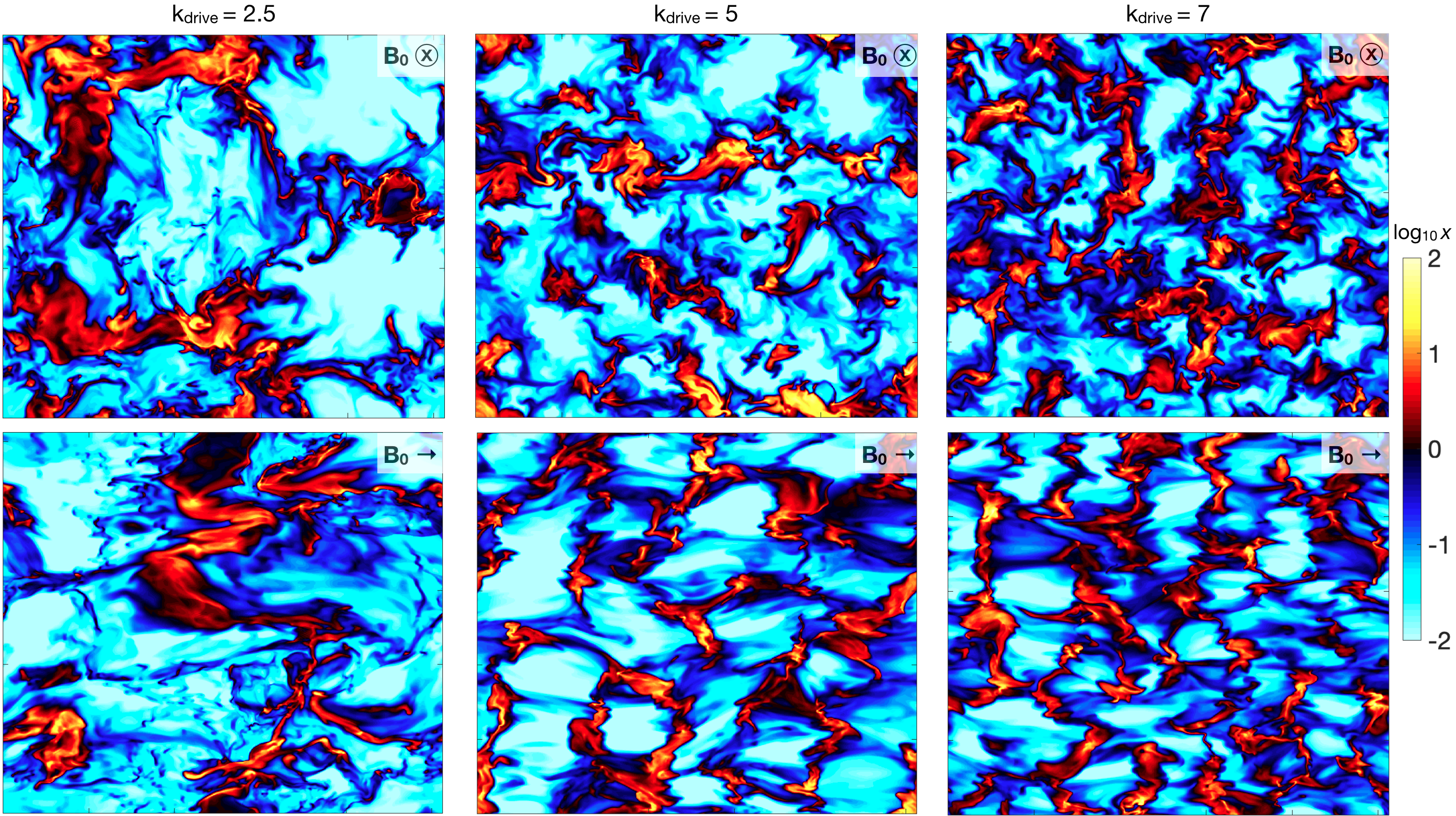
Folder $L_{\rm drive}$ contains the numerical simulations used in the Bialy & Burkhart (2020) study. These simulations are uniform grid density files (in FITS format) at resolution 256³, similar to those described in the setup in Folder 256 but with different driving scales. We include simulations with driving scales $k=2.5,k=5$ and $k=7$. These simulations have sonic Mach number $\mathcal{M}_{\rm s}=7.0$ and Alfvénic Mach number $\mathcal{M}_{\rm A}=0.7$. We show slices of the simulations with different driving scales in Figure 2. Please cite Bialy & Burkhart (2020) when using these simulations. Higher-resolution runs (512³ and 1024³) are available on request.

Figure 2.— Density slices through simulations with different driving scales. The driving scales are at $k=2.5$ (left), $k=5$ (middle) and $k=7$ (right). The top panel shows the mean magnetic field along the axis of density integration and the bottom panel shows the density integration perpendicular to the mean magnetic field. Reproduced with permission from Bialy & Burkhart (2020).

2.1.3 Cho-ENO MHD Simulations: HI-to-H₂ Transition and Synthetic HI Observations

The atomic-to-molecular (HI-to-H₂) transition is a key physical process that takes place in the ISM of galaxies (e.g. Savage et al., 1977; Gnedin et al., 2009; McKee & Krumholz, 2010; Lee et al., 2012; Sternberg et al., 2014; Bialy et al., 2015, 2017). The HI-to-H₂ transition may be important for the cooling and regulation of star formation (especially in the early universe), and it is also a necessary step for the formation of a wealth of other molecules, e.g., CO, OH, and H₂O (Bialy et al., 2015), as well as more complex molecules (Tielens, 2013).

Bialy et al. (2017) modeled the HI-to-H₂ transition in a turbulent medium irradiated by FUV fluxes. The transition from atomic to molecular form occurs as the FUV radiation is absorbed by dust and also occurs in H₂ line excitation (and dissociation). The role of turbulence is to create density fluctuations, which in turn have a strong effect on the HI-H₂ structure of the gas. Bialy et al. (2017) showed that the sonic Mach number and the driving length scale of turbulence directly affect the distribution of the HI column density at the edges of a molecular cloud, where the dispersion of the HI column density distribution increases with increasing Mach number and with increasing turbulence driving scale. Moreover, Micic et al. (2012) investigated the role of the turbulence driving for H₂ formation and found that compressive (curl-free) driving of the turbulence is much more efficient at producing molecular gas than solenoidal (divergence-free) driving. This, and the work by Bialy et al. (2017), suggests that observations of HI may potentially be used to constrain turbulence properties in the ISM.

Bialy et al. (2017) produced HI column density maps (units: cm^-2) for Cho-ENO MHD turbulent boxes using a similar setup as presented above by irradiating the numerical box with an isotropic or beamed ultraviolet (UV) field and applying the HI-H₂ (atomic to molecular hydrogen) formalism of Sternberg et al. (2014) and Bialy & Sternberg (2016). This procedure turns the simulation into a synthetic observation that can be used to study HI-H₂ physics in the presence of a turbulent medium as well as allowing for comparison with observations.

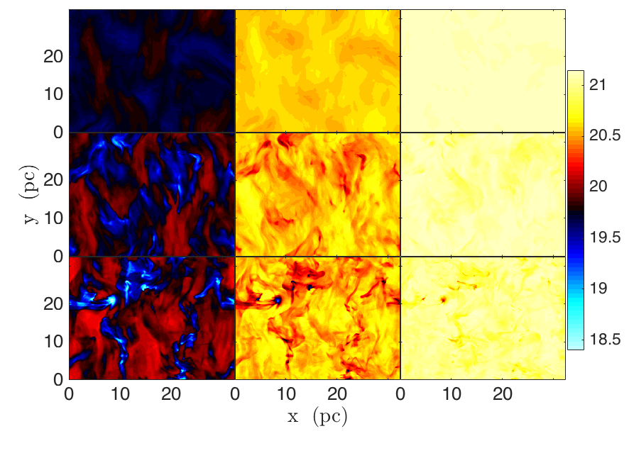
The basic setup of these synthetic observations is the following: UV radiation photo-dissociates molecular hydrogen and produces an atomic hydrogen layer at the cloud boundary. The HI column density of this layer depends on the UV intensity, gas density and dust absorption cross section. As shown by Bialy et al. (2017), the HI column density also depends on the properties of the turbulence. Turbulence produces density fluctuations in the gas, which alter the H₂ formation efficiency and self-shielding, thus resulting in fluctuations in the HI and H₂ column density for different lines of sight (Bialy et al., 2017). We provide results for simulations with sonic Mach number $\mathcal{M}_{\rm s}=4.5$ and Alfvénic Mach number $\mathcal{M}_{\rm A}=0.7$. The assumed physical parameters represent those typical to the Milky Way galaxy, with: 1) the UV intensity relative to the Draine (1978) field $I_{\rm UV}=1.3$, 2) the dust absorption cross section in the Lyman-Werner band $\sigma_{g}=1.9\times 10^{-21}$ cm², 3) a mean density of the cold neutral medium $n=30$ cm^-3, and 4) the ratio of the density decorrelation scale to the HI layer scale $L_{\rm dec}/L_{\rm HI}=0.1$, i.e., on average there are $\sim$ ten density fluctuations along the HI column. We ask that Bialy et al. (2017) please be cited when using these synthetic observations. We show visualizations of the HI column density maps in Figure 3. Additional runs with other parameter sets may be supplied upon request. In addition, columns and abundances of other molecules (H₂, OH⁺, H₂O⁺, ArH⁺) are also available upon request. (See Bialy et al., 2019).

2.1.4 3-point Correlation Function

Portillo et al. (2018) calculated the 3PCF of Cho-ENO MHD turbulent boxes using the Fourier Transform-based approach presented in Slepian & Eisenstein (2016). The 3PCF is the excess, over and above a spatially random distribution, of density at the vertices of triangles of a given shape and includes phase information that is missed in the 2-Point Correlation Function or power spectrum. For a density field $\delta(\boldsymbol{x})$, the 3PCF, denoted $\zeta$, can be written as a function of two triangle side lengths $r_{1}$ and $r_{2}$ and the cosine of the angle between them, $\hat{r}_{1}\cdot\hat{r}_{2}$,

$$\zeta(r_{1},r_{2};\hat{r_{1}}\cdot\hat{r_{2}})=\left<\delta(\boldsymbol{x})\delta(\boldsymbol{x}+\boldsymbol{r_{1}})\delta(\boldsymbol{x}+\boldsymbol{r_{2}})\right>$$ (4)

where the angle brackets average over all triangles of fixed shape set by $r_{1}$, $r_{2}$, and $\theta_{12}$, but with any position $\boldsymbol{x}$ for their vertex. Slepian & Eisenstein (2016) present a fast method to calculate the 3PCF in the Legendre basis where the angle dependence is written in terms of the Legendre polynomials $P_{\ell}$:

$$\bar{\zeta}(r_{1},r_{2};\hat{r}_{1}\cdot\hat{r}_{2})=\sum_{\ell}\bar{\zeta}_{\ell}(r_{1},r_{2})P_{\ell}(\hat{r_{1}}\cdot\hat{r_{2}}),$$ (5)

and the radial dependence is computed on bins described by a binning function $\Phi$:

$$\bar{\zeta}_{\ell}(r_{1},r_{2})=\int_{r\in\Phi(r_{1})}r^{2}dr\int_{r^{\prime}\in\Phi(r_{2})}r^{\prime 2}dr^{\prime}\;\zeta_{\ell}(r,r^{\prime}).$$ (6)

The bars denote that we are obtaining the full 3PCF (and the radial coefficients) binned onto spherical shells.

We provide 3PCFs calculated up to $\ell_{\rm max}=5$ for $N_{\rm b}=32$ radial bins of a constant width of 4 simulation voxels, so that the largest bin probes scales up to 128 voxels, half the simulation box size. On scales larger than half the simulation box we would expect the periodic boundary conditions to cause an order-unity effect, and so the simulation should not be trusted on those scales. There is a 3PCF file for each Cho-ENO simulation, with $\delta(\boldsymbol{x})$ being the log of the density fluctuations, i.e., $\delta=[\ln\rho-\left<\ln\rho\right>]/\sigma(\rho)$, where $\sigma(\rho)$ is the density standard deviation. Each file is an $(\ell_{\rm max}+1)\times N_{\rm b}\times N_{\rm b}$ numpy array representing $\bar{\zeta}_{\ell}(r_{1},r_{2})$ with $\ell$ running from 0 to $\ell_{\rm max}$ over the first index and the radial bins running over the other indices. We note that it can be useful to scale $\bar{\zeta}$ by the product of the number of voxels in both radial bins, which scales as roughly $r_{1}^{2}r_{2}^{2}$, so we include the number of voxels in all bins as a separate file. Since the cubic grid is discrete, one must actually count the number of voxels in each bin; it is not precisely $r_{1}^{2}r_{2}^{2}$ and hence cannot be divided out analytically. Further details are in Portillo et al. (2018). Please cite Portillo et al. (2018) when using these data products.

Figure 3.— Visualization of the synthetic HI column density maps produced from the Cho-ENO simulations. The color bar is $\log_{10}$($N_{\rm HI}$), and the 9 panels correspond to models with $\mathcal{M}_{\rm s}=0.5$, $2$, $4.5$ (from the top row to the bottom row, respectively) and $I_{\rm UV}=0.1$, $1$, $10$ (from the first column to the last column, respectively).

2.2. arepo Moving Mesh Simulations

We release a simulation suite of solenoidally driven supersonic isothermal magnetized turbulent boxes with parameters relevant to the ISM on parsec scales in dense molecular clouds, as simulated in Mocz et al. (2017) and Mocz & Burkhart (2018) with the arepo code. arepo (Springel, 2010) is a moving mesh quasi-Lagrangian code which solves the ideal MHD equations with an unstructured vector potential constrained transport solver (Yee, 1966; Evans & Hawley, 1988; Mocz et al., 2016) to maintain the divergence-free property of the magnetic field. Shocks are captured via the use of a Harten-Lax-van Leer Discontinuities (HLLD) (Miyoshi & Kusano, 2005) Riemann solver. In the arepo simulations, turbulence is driven in a purely solenoidal (divergence-free) manner in Fourier space on the largest spatial scales using an Ornstein-Uhlenbeck process (Federrath et al., 2010; Bauer & Springel, 2012; Federrath, 2015). Snapshots are provided for the properties of the turbulent gas both with and without self-gravity switched on. Self-gravity is calculated using a Tree-Particle-Mesh hybrid scheme (Xu, 1995) and leads to the collapse of pre-stellar cores in this physical setup.

Mocz et al. (2017) ran four isothermal simulations (adaptive $256^{3}$ resolution) with parameters relevant for representing a large region of a giant molecular cloud (GMC), exploring the effect of the (invariant) mean magnetic field $B_{0}$ threading the system. The turbulence is characterized by a sonic Mach number of $\mathcal{M}_{\rm s}\simeq 10$. The mean magnetic field (four cases simulated) is characterized by the corresponding plasma-beta $\beta_{0}$ or, equivalently, the Alfvénic Mach number $\mathcal{M}_{{\rm A},0}$ of the mean-field: $\beta_{0}=25,0.25,0.028,0.0025$ or, equivalently, $\mathcal{M}_{{\rm A},0}=35,3.5,1.2,0.35$. The simulations span from very weak seed fields to strong fields whose energy density surpasses the turbulent kinetic energy density. The simulation set establishes quasi-steady state turbulence (indicated by file names with 00), followed by the results obtained when self-gravity is switched on. Gravity leads to the formation of pre-stellar cores whose collapses are resolved from the GMC parsec scales down to the end of the isothermal collapse (AU scales). The collapse occurs on the order of the gravitational free-fall time of the cloud.

The sonic and Alfvénic mean-field Mach numbers completely characterize the system without gravity. With gravity switched on, the simulations may be further characterized by a dimensionless virial parameter, $\alpha_{\rm vir}=5v_{\rm rms}^{2}(L/2)/(3GM)=1/2$, where $L$ is the length of the system and $M$ is the total mass. The virial parameter describes the strength of the turbulent kinetic energy relative to gravitational potential energy. The simulations can be appropriately rescaled to different units as long as these dimensionless parameters are held fixed (McKee et al., 2010).

The physical parameters of the 4 simulations (assuming a mass per hydrogen of $1.4~{}{\rm amu}$) scale as:

$$L_{0} =5.2\left(\frac{c_{\rm s}}{0.2~{}{\rm km}~{}{\rm s}^{-1}}\right)\left(\frac{n_{H}}{10^{3}~{}{\rm cm}^{-3}}\right)^{-0.5}\left(\frac{\mathcal{M}_{\rm s}}{10}\right)~{}{\rm pc}$$ (7)

$$B_{0} =\{1.2,12,36,120\}\times\left(\frac{c_{\rm s}}{0.2~{}{\rm km}~{}{\rm s}^{-1}}\right)\left(\frac{n_{H}}{10^{3}~{}{\rm cm}^{-3}}\right)^{0.5}{\rm\mu G}$$ (8)

$$M =4860\left(\frac{c_{\rm s}}{0.2~{}{\rm km}~{}{\rm s}^{-1}}\right)^{3}\left(\frac{n_{H}}{10^{3}~{}{\rm cm}^{-3}}\right)^{-0.5}\left(\frac{\mathcal{M}_{\rm s}}{10}\right)^{3}M_{\odot}$$ (9)

where $L_{0}$ is the size of the periodic box with a total mass of $M$.

The arepo simulations are presented as snapshot HDF5 files that contain fields in the original unstructured Voronoi mesh. We include full snapshot data of $256^{3}$ resolution runs. 00 in the file name indicates a run with developed MHD turbulence but no gravity. Gravity is then switched on for later snapshots. Two snapshots are included for each run. We supplementally include re-gridded uniform mesh snapshots as part of the release. The CATS AREPO release also includes a sample jupyter notebook that demonstrates how the data can be loaded into yt. At the time of this publication, yt does not explicitly support arepo simulation data, although that functionality is expected to be added soon. arepo data is read into yt as gadget particle data, assuming an adaptive smoothing length that scales as the cube root of each Voronoi cell volume.

Figure 4 highlights two illustrative cases of the simulation suite of Mocz et al. (2017).

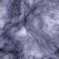
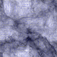
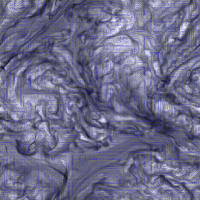
Two representative arepo simulations from Mocz et al. (2017) 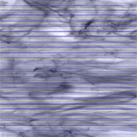weak mean-field ($\mathcal{M}_{\rm A,0}=35$) strong mean-field ($\mathcal{M}_{\rm A,0}=0.35$) (projections $\parallel$ & $\perp$ to mean-field)

Figure 4.— Visualization of two illustrative cases of arepo supersonic isothermal turbulent simulations from Mocz et al. (2017). Shown are density projections perpendicular and parallel to the mean magnetic field along with synthetic UV polarization vectors for a weak magnetic field simulation (left) and a strong field simulation (right). Also included in the simulation suite are intermediate field strengths and simulations with self-gravity, which resolve the collapse of pre-stellar cores (not shown).

2.3. enzo Simulations

2.3.1 Driven Turbulent Box Simulations with Self-gravity

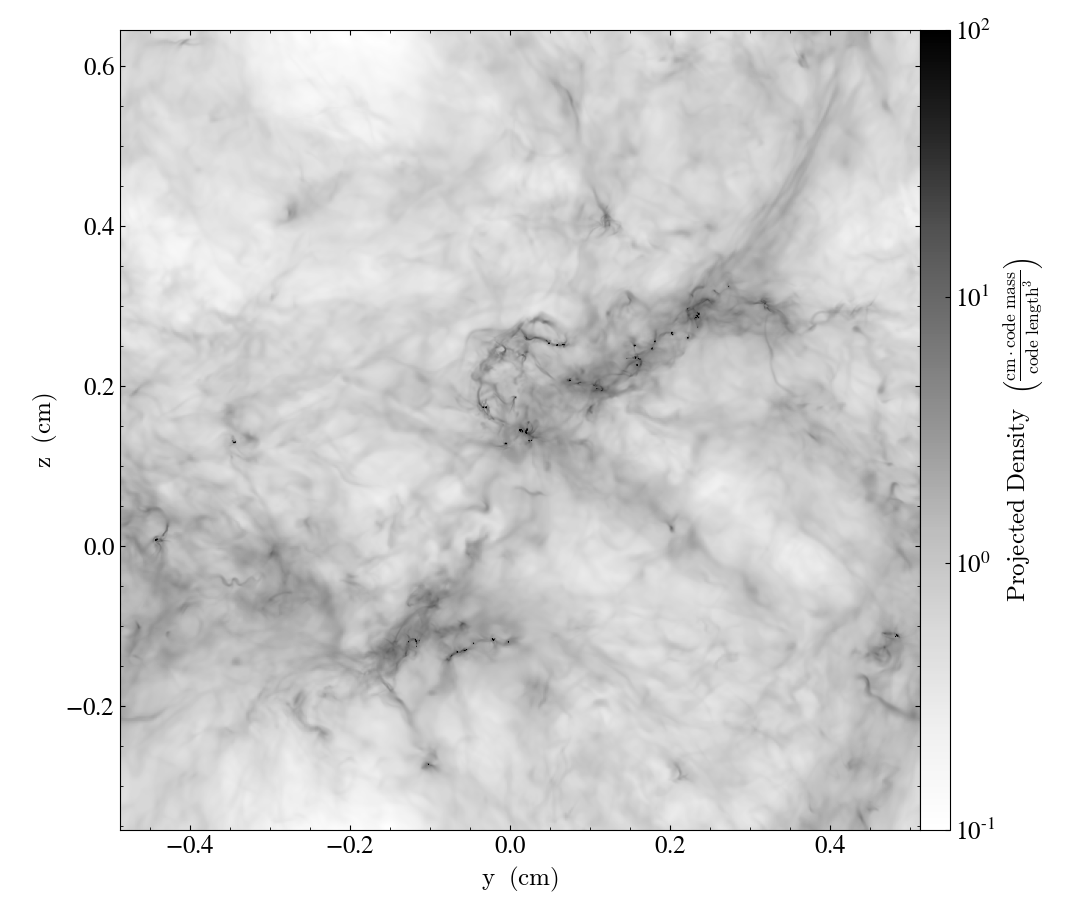
CATS includes simulations that were first presented in Collins et al. (2012) and employ isothermal, self-gravitating MHD with three values of the mean magnetic field. Projections of the three simulations can be seen in Figure 5. These datasets used the enzo (Bryan et al., 2014) code, extended to MHD by Collins et al. (2010). This code uses adaptive mesh refinement (AMR) algorithms developed by Berger & Colella (1989) and Balsara (2001), the hyperbolic solver of Li et al. (2008), the isothermal HLLD Riemann solver developed by Mignone (2007), and the constrained transport method of Gardiner & Stone (2005) to keep the divergence of the magnetic field to zero. The root grid is 512 zones on a side. Resolution is added adaptively whenever the local Jeans length, $L_{\rm{J}}=\sqrt{c_{\rm{s}}^{2}\pi/G\rho}$, is resolved by at least 16 zones (which avoids artificial fragmentation and allows us to resolve turbulence on the Jeans scale fairly well; see Truelove et al., 1997; Federrath et al., 2011). This gives an effective linear resolution of 8,192 zones. The simulations were run for $0.6t_{\rm{ff}}$, where the cloud-averaged free-fall time is $t_{\rm{ff}}=(3\pi/32G\rho_{0})^{1/2}$.

The simulations from Collins et al. (2012) employ both turbulence and self-gravity with similar Mach numbers as the arepo runs. For the enzo simulations, we select the Mach number, $\mathcal{M}$, virial parameter, $\alpha_{\rm{vir}}$, and mean thermal-to-magnetic pressure ratio, $\beta_{0}$, as

$$\mathcal{M} =\frac{v_{\rm{rms}}}{c_{\rm{s}}}=9,$$ (10)

$$\alpha_{\rm{vir}} =\frac{5v_{\rm{rms}}^{2}}{3G\rho_{0}L_{0}^{2}}=1,$$ (11)

$$\beta_{0} =\frac{8\pi c_{\rm{s}}^{2}\rho_{0}}{B_{0}^{2}}=0.2,2,20,$$ (12)

where $v_{\rm{rms}}$ is the root mean square velocity fluctuation, $c_{\rm{s}}$ is the sound speed, $\rho_{0}$ is the mean density, $L_{0}$ is the size of the box, and $B_{0}$ is the mean magnetic field. In code units, $\rho_{0},$ $L_{0}$, and $c_{\rm{s}}$ are all set to unity, and the mean magnetic fields are $B_{0}=3.16,\;1$, and $0.316$. Note that in code units, Heaviside-Lorentz units are used, which removes a $4\pi$ from the MHD equations. Consequently, the magnetic code units differ from cgs units by $\sqrt{4\pi}$ in addition to the rest of the unit scaling.

We set the sound speed to be $c_{\rm{s}}=0.2\rm{km\ s^{-1}}$, the hydrogen number density to be $n_{\rm{H},3}=n_{H}/(1000\rm{cm}^{-3})$ and the mean molecular weight to be 2.3 amu per particle. The simulations may be re-scaled using the following relations:

$$t_{\rm{ff}} =1.1n_{\rm{H},3}^{-1/2}\;\rm{Myr},$$

$$L_{0} =4.6c_{\rm{s},2}n_{\rm{H},3}^{-1/2}\;\rm{pc},$$

$$v_{\rm{rms}} =1.8c_{\rm{s},2}\;\rm{km\ s^{-1}}$$

$$M =5900c_{\rm{s},2}n_{\rm{H},3}^{-1/2}\;M_{\odot},$$

$$B_{0} =\{13,4.4,1.3\}c_{\rm{s},2}n_{\rm{H},3}^{1/2}\;\mu\rm{G}.$$ (13)

The initial conditions for these simulations were generated by a suite of uniform grid simulations using the piecewise parabolic method on a local stencil (PPML code) (Ustyugov et al., 2009) without self-gravity. Cubes with $1024^{3}$ zones, with initially uniform density and magnetic fields, were driven solenoidally. Power in the driving was between wavenumbers $1\leq k/k_{\rm{min}}\leq 2$ and driven as in Mac Low (1999) to maintain the target Mach number. A full description of this initial turbulent phase can be found in Kritsuk et al. (2009). The simulations were then re-gridded to $512^{3}$ in a manner that preserved momentum and magnetic flux, and restarted with self-gravity.

Three snapshots for each of the three simulations are stored in the CATS repository, at $t=0.1,\ 0.3$, and $\ 0.6\ t_{\rm{ff}}$. The initial $0.1t_{\rm{ff}}$ is ignored as the early evolution retains a significant imprint of the higher-resolution initial conditions, but no substantial effects of self-gravity are seen at this time. For ease of analysis and data acquisition, fixed resolution cubes at $256^{3}$ are stored online. Higher-resolution snapshots, with resolution fixed at $512^{3}$, and the full AMR snapshots are available upon request, though these are much larger files (8 GB and 13 GB, respectively). The data are stored in code units as described above. To simplify units and manipulation, there is a script that accompanies the datasets that will load the data from the file and, if desired, create a dataset for use with the python-based code package yt.

When using these simulations in scientific work, please cite Collins et al. (2010, 2012) as well as this release paper.

Figure 5.— Projections of the density field from the enzo core formation simulation. Left to right, $\beta=0.2,2,$ and 20, respectively.

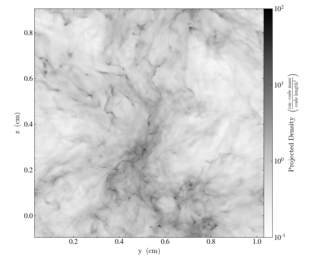
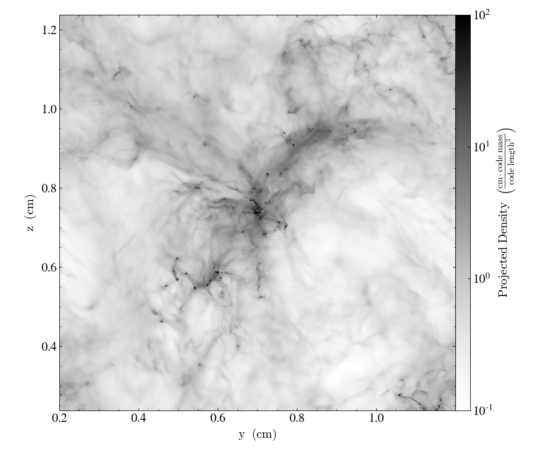
2.3.2 Hydrodynamic Simulations of Type Ia Supernova-driven Turbulence in a Hot Medium of Early-type Galaxies

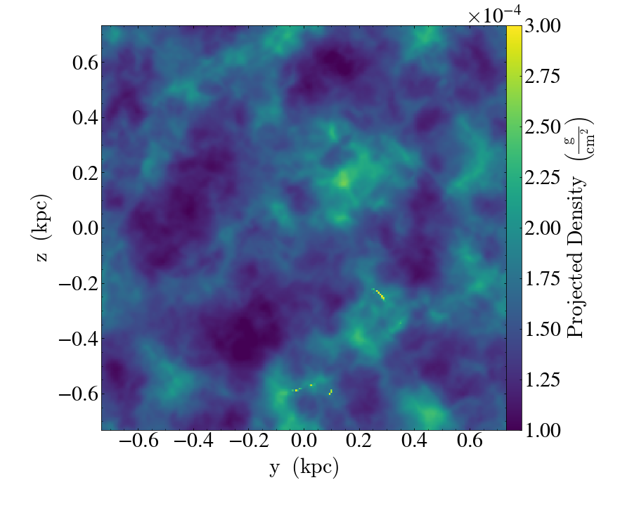
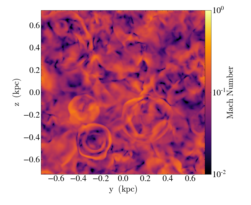
The simulations provided by Li et al. (2020a) are also run using the Eulerian code enzo. These simulations were set up to investigate how Type Ia SNe (SNe Ia) impact the thermal and dynamical properties of the medium in early-type galaxies. The ISM in these systems is hot and tenuous, with a temperature range of $10^{6}$–$10^{8}$ K and a density range of $10^{-3}$–$1$ cm^-3. The ISM condition is therefore very different from that in star-forming galaxies.

The simulations utilize a 3D uniform grid with periodic boundary conditions. The hydro solver is the finite-volume piecewise parabolic method (Colella & Woodward, 1984). The fiducial runs have $128^{3}$ cells and the high-resolution runs have $256^{3}$. The initial condition is a uniform and static medium. SNe Ia exploded randomly in the box at a constant rate. The sizes of the simulation box and the injection zones are chosen based on the fade-away radius of an SN remnant, defined as the radius when the shock wave fades into a sound wave,

$$\begin{split}R_{\rm fade}&=\left((\gamma-1)\frac{E_{\rm{SN}}}{4\pi P/3}\right)^{1/3}\\ &=48.8~{}\rm{pc}\ E_{51}^{1/3}n_{0.02}^{-1/3}T_{7}^{-1/3},\end{split}$$ (14)

where $P$, $n$, and $T$ are the pressure, number density, and temperature, respectively, of the ambient gas, $E_{\rm{SN}}$ is the energy released by an SN, $\gamma$ is the adiabatic index, $T_{7}=T/10^{7}$K, $n_{0.02}=n/0.02$ cm^-3, and $E_{\rm{51}}=E_{\rm{SN}}/10^{51}$erg.

The box length is chosen to be $20\,R_{\rm SN}$. Each SN has a spherical injection zone with a radius of 0.5$R_{\rm{fade}}$, so the remnant evolution is resolved. The injection is implemented by taking $E_{\rm{SN}}=10^{51}$ erg thermal energy, $m_{\rm{SN}}=$ 1 $M_{\odot}$, and a fixed amount of “color” (passive scalar) that follows the mass flux. These quantities are evenly distributed in the injection zone. Note that $R_{\rm fade}$ depends on the gas pressure, so for runs with different gas pressure the box sizes and injections zones are adjusted according to Equation 14. The only driving forces for the turbulence are the SNe.

Radiative cooling is included by using a cooling curve (Rosen & Bregman, 1995). The simulations are run for four cooling times of the initial hot medium. A run is uniquely identified by the thermal properties of the medium and the SNe explosion rate. Gas density, temperature and SN explosion frequencies are varied for different simulation boxes for a parameter study. More details on this setup can be found in Li et al. (2020a).

SNe Ia heat the ISM and drive turbulence into the hot medium. SNe feedback in these galaxies is distinguished from that in star-forming galaxies by the fact that the blast waves driven by SNe do not have a cooling phase and therefore do not form a thin shell, but rather fade directly into a sound wave. Li et al. (2020a) investigated the formation of the cool phase in the hot medium. They found that due to the stochastic nature of the SNe Ia explosions, patches of the hot media not heated by any SNe cool down after an approximate cooling time. Turbulence delays the time of formation of the cool phase. Li et al. (2020b) examined the thermal structure and turbulence of the hot media under SNe. They have found that the SNe, together with the thermal instability of the hot gas, leave a broad log-normal distribution of density (e.g., Körtgen et al., 2019). SNe drive a mild subsonic turbulence. The velocity structure is dominated by compressional, rather than solenoidal, motions. This is different from what occurs in star-forming galaxies (e.g. Korpi et al., 1999; Balsara et al., 2004a; Käpylä et al., 2018). The reason is that in an ISM of an early-type galaxy, the frequency of SNe explosions is low and the interaction among SNe remnants is lacking. As a result, the spherical blast waves are not converted into solenoidal motions.

Furthermore, in an isothermal turbulent medium, there is a simple correlation between the density fluctuation and the Mach number. The following ratio is generally found to be in the range of 1/3–1 (Padoan et al., 1997; Federrath et al., 2008, 2010; Konstandin et al., 2012):

$$b\equiv\frac{\sigma_{\rho,V}}{\bar{\rho}_{V}}/\mathcal{M}_{\rm s},$$ (15)

where $\bar{\rho}_{V}$ is the volume-weighted mean density, $\sigma_{\rho,V}$ is the volume-weighted standard deviation of density, and $\mathcal{M}_{\rm s}$ is the RMS Mach number. In contrast, in the hot medium under SNe Ia, this ratio is found to be continuously growing due to thermal instability, reaching 4-20 within a few cooling times.

For enzo simulations, the output data can be accessed and analyzed using yt . A few example runs are included on the CATS website, each including several snapshots. The naming of the runs indicates the initial condition and the SNe heating rate, e.g., n0.02_T1e7K_H1.02C indicates that the initial condition has density $n=0.02~{}{\rm cm}^{-3}$, temperature $T=10^{7}~{}{\rm K}$, and SNe heating rate $1.02$ times the cooling rate of the medium. If present, hr indicates that the run is a high-resolution run. More data is available upon request. For a full list of the runs, see Table LABEL:table.summary of Li et al. (2020a).

When using these simulations, please cite the following papers: Li et al. (2020a, b) and this release work.

Figure 6.— Projection of the density and slice of the local Mach number from an exemplar run in Li et al. (2020a).

2.4. flash Simulations

flash is an Eulerian, AMR, MHD code (Fryxell et al., 2000; Dubey et al., 2012) that provides a choice of various approximate Riemann solvers for hydrodynamics and MHD. Available physics modules include self-gravity, external gravity, radiative cooling, diffuse heating from far UV, sink particles for star formation, and turbulent driving.

2.4.1 flash Multiphase Interstellar Medium Simulations

Figure 7.— Images of number density in a midplane slice (left) and a vertical slice (right) from the bx5 pe300 2pc simulation of Hill et al. (2018). We show magnetic field vectors with length proportional to $|\vec{B}|$.

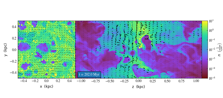
Hill et al. (2018) used flash version 4.2 to run simulations of SN-driven hydrodynamical and MHD turbulence in a stratified, multi-phase section of a galactic disk (neglecting background shear), varying the diffuse heating rate to study the resulting structure of the interstellar medium. The Riemann solver used is the positivity-preserving, directionally-split HLL3R implementation of Waagan et al. (2011). The models are described fully elsewhere (Joung & Mac Low, 2006; Joung et al., 2009; Hill et al., 2012, 2018), and we show an image of a slice from one model in Figure 7.

These models were run on a rectangular base grid $1\times 1\times 40$ kpc in size, centered on the midplane of the Galaxy and extending $|z|=20$ kpc above and below the midplane. The maximum grid refinement varies with height, reaching values as small as $\Delta x=0.98$ pc in the innermost 100 pc, and then increasing as shown in Table 2 of Hill et al. (2012). Periodic boundary conditions were used on the sides, and a zero-gradient outflow boundary condition at the top and bottom, though only a small percentage of the mass ultimately leaves the vertical boundaries. The gas starts in hydrostatic equilibrium with a static background potential described by Hill et al. (2018), with the innermost kiloparsec above and below the midplane having a temperature $T=1.15\times 10^{4}$ K and gas beyond that being given coronal temperatures of $T=1.15\times 10^{6}$ K. We assume the gas has a uniform mean mass per hydrogen atom of $\mu=2.36\times 10^{-24}$ g, so that the number density $n=\rho/\mu$, where $\rho$ is the mass density of the gas.

These models include a diffuse heating rate $\Gamma(T,z)$, modeling photoelectric heating by far UV photons, and a fixed cooling curve $\Lambda(T)$, modeling collisionally ionized plasma. The balance between these heating and cooling terms establishes a two-phase ISM. The energy density $e$ then evolves as

$$\partial e_{t}=n\Gamma(z,T)-n^{2}\Lambda(T).$$ (16)

The value of $\Gamma$ drops off exponentially in the vertical direction with a scale height of 8.5 kpc (high enough that $\Gamma$ varies little within the galactic disk and inner halo). The photoelectric heating term is only applied to gas with temperature $T<2\times 10^{4}$ K, as hotter gas quickly sputters the dust that provides the photoelectrons. The cooling curve we have chosen results in a multiphase thermal equilibrium for pressures

$$P/k\in([670,8300]\mbox{ K cm}^{-3})(\Gamma/10^{-25}\mbox{ erg s}^{-1}).$$ (17)

Multiple populations of SNe are included, each injecting $10^{51}$ erg of energy into 60 M_⊙ of gas, along with an approximate treatment of early stellar winds in clusters. SNe are set off at prescribed times based on an average Galactic SN rate with random locations, as the lack of self-gravity and other physical processes important to star formation means we do not meaningfully model star formation. Type Ia SNe are 19% of the total SN rate, and are given a scale height of $H=300$ pc; field core-collapse SNe are 32%, with $H=90$ pc; and clustered core-collapse SNe are 47%, also with $H=90$ pc. The clustered SNe occur in groups of 7–40 SNe spread over 40 Myr, simulating the evolution of OB associations. In these locations, we begin by injecting an SN’s worth of thermal energy continuously over 5 Myr to model the prompt clearing of gas by stellar winds from OB associations. SNe and clusters are randomly placed with respect to density concentrations, resulting in clouds living for unphysically long times (Hill et al., 2018). Shocks from SNe heat the gas to $\gtrsim 10^{6}$ K and establish the third phase in the multiphase ISM.

This parameter study focuses on the effect of varying the diffuse far-UV heating rate from 1.09–12.3 $\times 10^{-25}$ erg s^-1, as described in Table 1 of Hill et al. (2018), while also varying a small number of other parameters, including the initial magnetic field (either 0 or 5 $\mu$G in the $\hat{x}$-direction), the finest numerical resolution (0.98 to 7.81 pc, corresponding to $1024^{3}$ to $128^{3}$ in the plane), the gas surface density (7.5 to 13.4 M_⊙ pc^-2), and the SN rate (17.1 or 34.1 Myr^-1 kpc^-2). In all cases, we began by running low-resolution runs ($\Delta x=7.81$ pc) for 160 Myr to establish the galactic fountain flow. We then improved the resolution in steps, reaching $\Delta x=3.91$ pc at 180 Myr, $\Delta x=1.95$ pc at 190 Myr, and, in the run with the highest heating rate, $\Delta x=0.980$ pc at 190 Myr. The lower-resolution runs were also continued to 200 Myr to enable resolution studies.

CATS includes output from the models listed in Table LABEL:table.summary of Hill et al. (2018), along with example python code to read the HDF5 files using yt (Turk et al., 2011). The output files are HDF5 files that include all field variables for each of these runs at a time of $t=200$ Myr, when they have reached dynamical equilibrium, providing models for ISM turbulence in both the plane and the fountain flow of the galaxy. Please cite Hill et al. (2018) and this CATS paper if these data are used.

2.4.2 flash Zoom-in Molecular Cloud Simulations

Ibáñez-Mejía et al. (2016) took MHD models of multiphase, supernova-driven, stratified turbulence that were identical to those presented in Sect. 2.4.1 (except as mentioned below), but that included gas self-gravity using the multigrid (Huang & Greengard, 1999) scheme implemented in flash (Ricker, 2008; Daley et al., 2012), in addition to a background galactic potential (described in Ibáñez-Mejía et al. (2016) in detail). These models were run with flash version 4.2.2. The self-gravity was only enabled after the evolution to a dynamical equilibrium, described in Sect. 2.4.1, had completed at $t=230$ Myr, after the explosion of over 7500 SNe. In a subsequent paper, Ibáñez-Mejía et al. (2017) zoomed in on individual newly forming dense clouds, increasing the maximum numerical resolution within collapsing regions to as high as $\Delta x=0.06$ pc. This provides data on the structure and evolution of a dense cloud embedded within a turbulent background having thermal and dynamical structure characteristic of the ISM. This contrasts with the assumption of many models of either a periodic box or a uniform sphere as the initial condition.

These models focus on ISM conditions at the solar circle, with surface density $\Sigma=13.7M_{\odot}$ pc^-2 and an SN rate of 34 Myr^-1 kpc^-2, with the same distribution of types as in Sect. 2.4.1, but a slightly larger scale height for the Type Ia SNe of 325 pc. They all begin with a uniform magnetic field chosen to have plasma $\beta=2.5$ everywhere which then evolves under the influence of a local turbulent dynamo driven by the SNe (e.g. Balsara et al., 2004b). The mean mass per particle in these models is $\mu=2.17\times 10^{-24}$ g, assuming atomic hydrogen with helium fraction of 0.97 and 0.3% heavier elements. Superbubbles are given the local bulk gas velocity on formation, with a maximum of 20 km s^-1. (In retrospect, this assumption caused many superbubbles that were initialized in low-density regions to move too quickly, and sometimes even escape into the low halo.) The diffuse heating rate was calculated with the FUV flux from Draine (1978) of 1.7 times the Habing (1968) value, and a flux scale height of 300 pc.

Three clouds were chosen for zoom-in simulations from clouds that started to form earlier in a $\Delta x=0.47$ pc run than in a $\Delta x=0.95$ pc run during the last 5 Myr of a 15 Myr extension past $t=230$ Myr. The clouds had initial masses of 3, 4, and 8$\times 10^{3}$ M_⊙ at the moment self-gravity was activated, and final masses of a few $10^{3}$ to $10^{4}$ M_⊙; these are designated M3, M4, and M8 based on their initial mass. The chosen clouds were then re-simulated with $\Delta x=0.47$ pc within a 100 pc³ box centered on the cloud, while the resolution was reduced for reasons of computational cost to $\Delta x=1.90$ pc outside in the rest of the midplane (see Table 1 of Ibáñez-Mejía et al. 2017). Furthermore, within the zoom-in box, refinement was allowed to continue in dense regions in order to resolve the Jeans length with $n_{J}=4$ zones (Truelove et al., 1997) down to a resolution of $\Delta x=0.06$–0.12 pc, depending on the mass of the cloud. The runs were ended when more than half the mass of the cloud had exceeded the critical Jeans density at a resolution of $\Delta x$. Figure 8 shows shows a face-on projection of the box from the simulation with 0.47 pc resolution at the midplane, at the time when the target clouds were identified. The three target clouds are also shown in close-up windows.

Figure 8.— Column density of $\Delta x=0.47$ pc ISM simulation projected perpendicular to the Galactic midplane at the moment before self-gravity is turned on at $t=200$ Myr. The (100 pc)³ zoom-in boxes around the target clouds are superposed. Close-ups of the zoom-in boxes around each of the clouds are also shown (after about 5 Myr of evolution at higher resolution), with a black contour outlining the $n=100$ cm^-3 region. Reproduced with permission from Ibáñez-Mejía et al. (2017).

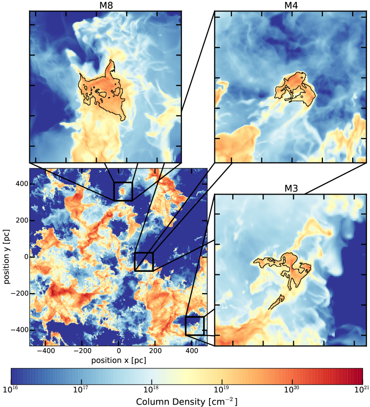
The files in CATS are HDF5 files including all field variables from these runs every 0.1 Myr from the start of the zoom-in calculation until the runs were stopped 4.9–6.2 Myr later. Example python code to read the HDF5 files using yt (Turk et al., 2011) and convert them to FITS using astropy (Astropy Collaboration et al., 2013) is also included. Please cite Ibáñez-Mejía et al. (2017), the archival repository (Chira et al., 2018), and this paper if these data are used.

2.4.3 flash MHD Turbulence Box Simulations

CATS includes MHD turbulent box simulations produced with flash version 4.6.2. Using flash, we solve the compressible MHD equations on three-dimensional (3D) periodic grids of fixed side length $L=2$ pc, including turbulence and magnetic fields. These simulations include a turbulence driving module that produces turbulence driven on large scales and forced with a large-scale k=1-3 parabolic forcing generator. We use a mixture of turbulence forcing and include a run that is fully solenoidal ($b=1/3$), fully compressive ($b=1$) and mixed driving ($b=1/2$) using the StirFromFile module in flash (Federrath et al., 2008, 2010), where $b$ indicates the forcing parameter. The different file names in the online folder show different values of $b$. We provide snapshots between 2-3 turnover times.

We include the flash.par parameter file that describes the parameter setup. With the exception of the forcing parameter, all other parameters of the turbulence are the same in these runs. The sonic Mach number is set at $\approx 7.5$ and the Alfvénic Mach number is set at $\approx 2$. The driving velocity amplitude is set to be $v_{\rm drive}=1.5~{}{\rm km}~{}{\rm s}^{-1}$ and the sound speed is $c_{\rm s}=0.2~{}{\rm km}~{}{\rm s}^{-1}$. When using these simulations in scientific work, please cite: Fryxell et al. (2000); Federrath et al. (2008, 2010); Federrath (2015), and this release work.

2.5. Athena++ Simulations

2.5.1 Radiative Mixing Simulations

Figure 9.— From left to right and top to bottom, slices of temperature ($T$), density ($\rho$), cooling time ($t_{\rm cool}$), pressure deviation ($\Delta P/\overline{P}$), $v_{x}$, $v_{y}$, $v_{z}$, and turbulent Mach number ($v_{\rm turb}/c_{\rm s}$) from the three-dimensional rapidly cooling athena++ turbulent mixing layer simulation. The background shear flow is in the $\hat{x}$ (horizontal) direction, with the hot gas moving to the right relative to the cold gas. The turbulence, traced by $v_{y}$, has induced mixing and broadened the shear velocity $v_{x}$, but the rapid cooling, localized entirely to a thin layer, maintains a sharp gradient between the cold and hot phases. The cooling leads to a flow of the hot gas into the cooling layer, $v_{z}<0$. Although the cooling is rapid, there is no signature of the cooling imprinted in the pressure field; instead, the pressure fluctuations correlate with turbulent fluctuations. An animated version of this figure is available here. Reproduced with permission from Fielding et al. (2020).

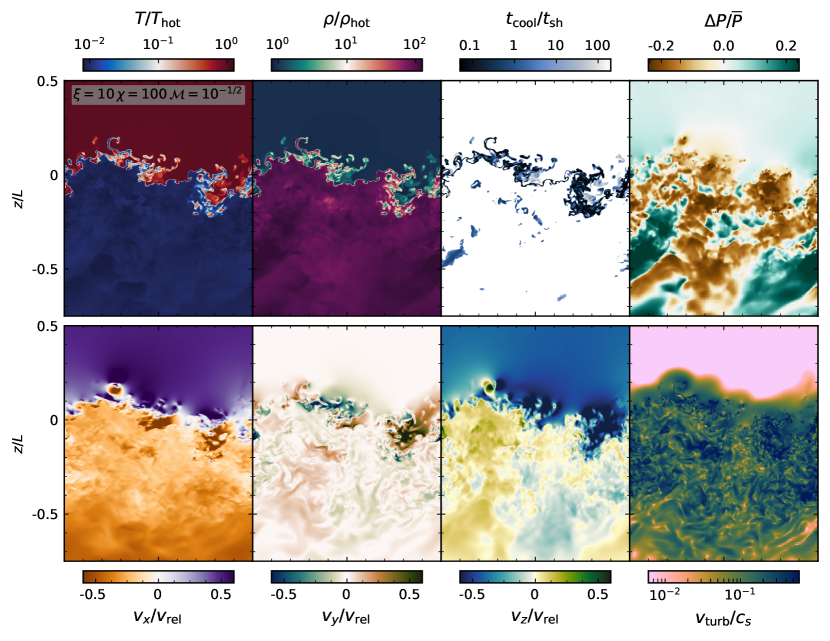
The CATS data release includes two three-dimensional hydrodynamic turbulent mixing layer box simulations run with the athena++ code framework and described in Fielding et al. 2020. One of the simulations includes strong radiative cooling, while the other does not. An example of the radiatively cooling simulation is shown in Figure 9. These simulations use a fiducial resolution of 128 cells per length ($L$) of the box, stream-wise length of the box and characteristic scale of the mixing layer. One of the provided simulations has no radiative cooling (in the directory, this run is labeled tshtcool00) and the other run has strong cooling, such that the cooling time is ten times shorter than the shear time (in the directory this run is labeled tshtcool10). In all other respects, the two simulations are identical.

The simulation domains are tall skinny boxes that are $L\times L\times 10L$ in shape. The initial conditions of the simulations have hot gas on top ($z>0$) and cold gas on bottom ($z<0$). The gas is in pressure equilibrium. The two phases are moving relative to each other. The relative velocity ($v_{\rm rel}$) of the hot and cold gas is in the $x$-direction and the gradient in the density and velocity is in the $z$-direction. The resolution is highest in the central $L\times L\times 3L$ region, outside of which the resolution rapidly decreases. These simulations have a density contrast of 100 (indicated by the chi100 label in the directory name) and relative velocity $10^{-0.5}=0.316$ less than the sound speed of the hot phase (indicated by the Mach03 label in the directory name). In code units, the pressure $P=1$, the relative velocity $v_{\rm rel}=0.41$, $L=1$, and the density of the hot phase $n_{\rm hot}=$ 1. The $x$ and $y$ boundary conditions are periodic. The $z$ boundary condition holds the density, pressure, and $x$ velocity constant while maintaining a zero gradient condition for the $y$ and $z$ velocities. There is an initial perturbation to the $z$ velocity that is 4% of the initial relative velocity. This perturbation has a sinusoidal component with wavelength equal to the box size and a white noise component that is imposed at the grid scale. There is no explicit conduction or viscosity.

In the radiative simulation, the hydro time-step is constrained to be less than one tenth of the shortest cooling time in the domain. The cooling rate of the material is set such that the cooling time of gas at intermediate temperatures is ten times shorter than the shear time ($t_{\rm sh}/t_{\rm cool}=10$, where $t_{\rm sh}=L/v_{\rm rel}$).

The simulation outputs are in HDF5 format. There are 100 outputs per simulation. All of the simulation parameters can be found in the included athinput.XXX.sh files. Information regarding the code-specific simulation parameters as well as useful analysis scripts can be found on the athena++ documentation page.

More detailed information on these simulations is available upon request or can be found in the primary reference. Visualizations of these simulations can be found here. When using these simulations in scientific works, please refer to and cite Fielding et al. (2020), the athena++ code paper Stone et al. (2020), and this data release paper.

3. Discussion

Shared community resources are increasingly critical for the reproducibility of scientific results and for progress. This is particularly true of fields that rely heavily on numerical simulations. Due to proprietary codes and large dataset sizes, numerical data products are often not released to the public. In this paper we have presented the CATS data release of astrophysical turbulence simulations, from a variety of codes that are free for public use.

Shared simulation resources such as CATS can benefit both theorists and observers dealing with problems surrounding astrophysical MHD turbulence. In general, the best strategy for studying a difficult subject like interstellar turbulence is to use a synergistic approach, combining theoretical predictions, numerical simulations, and observational data. In order to make sensible comparisons between theory, numerics, and astrophysical observations, statistical tools, post-processing of the simulations, and advanced data visualization tools are all necessary. Below we outline a few additional shared statistical, simulation, and visualization resources open to the community that are compatible with the CATS datasets and have been used in previous MHD turbulence studies.

3.1. Post-processing Tools: Synthetic Observations

MHD turbulence simulations provide 3D quantities such as density, magnetic field, and velocity that are not directly available through observations. Therefore, it is important to realize that simulations must be compared with observational data via the creation of synthetic observations. In practice, this often means a number of post-processing steps to transform the 3D idealized simulation into an apples-to-apples comparison with the observation and may include picking a line of sight and applying noise, beam smoothing, and radiative transfer. The output of the post-processing may be a column density map, polarization map, integrated intensity map, spectral line, or position-position-velocity data cube (Burkhart et al., 2013). For more applications to the diffuse ISM, turbulence simulations have also explored Synchrotron intensity and Synchrotron polarization fluctuations (Burkhart & Lazarian, 2012; Xu & Zhang, 2016; Kandel et al., 2016; Herron et al., 2016; Lazarian et al., 2017a).

More specifically, regarding radiative transfer application to the molecular ISM, a number of publicly available radiative transfer codes exist for MHD turbulence simulations. These include RADMC3D, Polaris, and DESPOTIC. RADMC3D is a radiative transfer code for dust and lines performed using a Monte Carlo method (Dullemond et al., 2012). Polaris is a well-established code designated for dust polarization and line radiative transfer in arbitrary astrophysical environments (Reissl et al., 2016, 2019). DESPOTIC is a library to Derive the Energetics and SPectra of Optically Thick Interstellar Clouds (Krumholz, 2014a).

Here we particularly highlight the DESPOTIC radiative transfer code, which has been applied to the enzo MHD molecular cloud simulations of Collins et al. (2012) included in this CATS data release paper. DESPOTIC’s capabilities include calculating spectral line luminosities from clouds of specified physical properties and compositions, along with determining their equilibrium temperatures and chemical compositions. DESPOTIC is implemented as a python package and its physical model, solutions to the equations it solves, and some tests and example applications are described in Krumholz (2014a). Most relevant for CATS, DESPOTIC can generate look-up tables of emissivity in a variety of molecular lines as a function of gas density and velocity using a range of physical assumptions, e.g., fixing the temperature versus solving for it self-consistently (Onus et al., 2018), or solving for the chemical composition while varying the cosmic ray ionization rate (Armillotta et al., 2020). These tables can then be used together with the analysis package yt (Turk et al., 2011) to generate synthetic position-position-velocity cubes from CATS data.

3.2. Statistical Analysis of Turbulence

As mentioned above, the best strategy for studying a difficult subject like interstellar turbulence is to use a synergistic approach, combining theoretical knowledge, numerical simulations, and observational data. Such a comparison can only be done in a meaningful way with the aid of statistics. While turbulence appears chaotic to the human eye, statistical properties of turbulence averaged temporally or spatially often display reproduciblity and regularity (Kowal & Lazarian, 2007; Kritsuk et al., 2007; Burkhart et al., 2015; Portillo et al., 2018).

Fortunately, there has been substantial progress in the development of techniques to study turbulence in the last decade. Techniques for quantifying aspects of turbulent flows can be tested empirically using parameter studies of numerical simulations and/or using analytic predictions. A statistical view of turbulence allows researchers to describe overall properties of the fluid flow. For astrophysical turbulence, these properties may include parameters that are important to this data release such as the injection and dissipation mechanisms, the strength and properties of the magnetic field (encapsulated by the Alfvénic Mach number) and the compressibility of the medium (encapsulated by the sonic Mach number).

An example of a more recently developed statistic for studying turbulent flows is the bispectrum and the related three-point correlation function. The bispectrum is the higher order analog to the power spectrum and is the Fourier transform of the 3-Point Correlation Function function (3PCF). Unlike the power spectrum, the bispectrum includes phase information, which allows correlations between different spatial frequencies/scales to be explored. Burkhart et al. (2009) and Burkhart & Lazarian (2016) demonstrated how mode-mode correlations change in different MHD turbulence regimes. More recently, the 3PCF was applied to similar simulations in Portillo et al. (2018). They used a fast multipole expansion algorithm introduced by Slepian & Eisenstein (2015) and extended to use Fourier Transforms (FTs) in Slepian & Eisenstein (2016). The 3PCF output of the Cho-ENO simulations presented in Portillo et al. (2018) is included in the CATS release (see Section 2.1.4), as well as ancillary code needed to interpret it.

Previously, there was no common framework for different turbulence statistics. Fortunately, a python-based statistics package called TurbuStat was publicly released specifically for application to astrophysical ISM observations (Koch et al., 2017, 2019). TurbuStat implements fourteen observational diagnostics of ISM turbulence described in the literature. TurbuStat provides a common framework for running and comparing turbulence diagnostics, including comparisons between simulations and observations.

3.3. Visualizing Data: ytini

In additional to performing statistical analysis, it is necessary to visualize simulation data. The datasets found on the CATS repository are compatible with a number of open source visualization tools. Excellent visualization packages include Glue (Beaumont et al., 2015) and yt (Turk et al., 2011). yt has been cited several times in the above simulation packages and therefore we will not discuss its many uses further.

Glue is an open-source software aimed at multi-dimensional data visualization and exploration. Equipped with various visualization approaches and selection schemes covering 1D, 2D, and 3D, Glue is distinguished by its linked-view paradigm which enables users to gain insight and understanding from complex models and datasets (Goodman, 2012). Glue has hybrid hackable user interfaces with both Graphic User Interface (GUI) and custom-written computer code ability. The GUI provides fluidity with a precision that enables it to perform specific common tasks very easily (Beaumont et al., 2015).

For simulation renderings and movies, the CATS data can also be used with the ytini package. ytini is a set of interfaces and tutorials designed to incorporate the scientific data-driven capabilities of yt into the industry standard special effects software Houdini (Naiman et al., 2017). By combining these software packages, an intuitive interface to render volumetric data with access to complex lighting, camera and coloring/shading techniques is provided for scientists to produce movie-quality scientific data visualizations. Figure 1 shows two rendered images of an example FITS density cube generated with ytini. A movie made by ytini of a CATS simulation may be found on the CATS website. A custom python reader has been created for CATS datasets and is detailed in a blog post on www.ytini.com.

4. Conclusions

In this data release paper we presented the Catalogue for Astrophysical Turbulence Simulations (CATS), a new database for open source compressible MHD turbulence simulations and related statistics. This data release paper represents our initial contributions, which will remain permanently up on the site. It is highly likely that the database will evolve over time and include additional contributions and simulations. For all contributions, a README file will be provided to explain the dataset and give examples of analysis and usage.

References

- Armillotta et al. (2020) Armillotta, L., Krumholz, M. R., & Di Teodoro, E. M. 2020, MNRAS, 493, 5273
- Armstrong et al. (1995) Armstrong, J. W., Rickett, B. J., & Spangler, S. R. 1995, ApJ, 443, 209
- Astropy Collaboration et al. (2013) Astropy Collaboration, Robitaille, T. P., Tollerud, E. J., Greenfield, P., Droettboom, M., Bray, E., Aldcroft, T., Davis, M., Ginsburg, A., Price-Whelan, A. M., Kerzendorf, W. E., Conley, A., Crighton, N., Barbary, K., Muna, D., Ferguson, H., Grollier, F., Parikh, M. M., Nair, P. H., Unther, H. M., Deil, C., Woillez, J., Conseil, S., Kramer, R., Turner, J. E. H., Singer, L., Fox, R., Weaver, B. A., Zabalza, V., Edwards, Z. I., Azalee Bostroem, K., Burke, D. J., Casey, A. R., Crawford, S. M., Dencheva, N., Ely, J., Jenness, T., Labrie, K., Lim, P. L., Pierfederici, F., Pontzen, A., Ptak, A., Refsdal, B., Servillat, M., & Streicher, O. 2013, A&A, 558, A33
- Ballesteros-Paredes & Hartmann (2007) Ballesteros-Paredes, J. & Hartmann, L. 2007, Rev. Mex. Astron. Astroph., 43, 123
- Balsara (2001) Balsara, D. S. 2001, J. Comput. Phys, 174, 614
- Balsara et al. (2004a) Balsara, D. S., Kim, J., Mac Low, M.-M., & Mathews, G. J. 2004a, ApJ, 617, 339
- Balsara et al. (2004b) —. 2004b, ApJ, 617, 339
- Bauer & Springel (2012) Bauer, A. & Springel, V. 2012, MNRAS, 423, 2558
- Bayliss et al. (2007) Bayliss, R. A., Forest, C. B., Nornberg, M. D., Spence, E. J., & Terry, P. W. 2007, Phys. Rev. E, 75, 026303
- Beattie & Federrath (2020) Beattie, J. R. & Federrath, C. 2020, MNRAS, 492, 668
- Beaumont et al. (2015) Beaumont, C., Goodman, A., & Greenfield, P. 2015, in Astronomical Society of the Pacific Conference Series, Vol. 495, Astronomical Data Analysis Software an Systems XXIV (ADASS XXIV), ed. A. R. Taylor & E. Rosolowsky, 101
- Beresnyak & Lazarian (2019) Beresnyak, A. & Lazarian, A. 2019, Turbulence in Magnetohydrodynamics (Walter de Gruyter)
- Beresnyak et al. (2005) Beresnyak, A., Lazarian, A., & Cho, J. 2005, ApJ, 624, L93
- Berger & Colella (1989) Berger, M. J. & Colella, P. 1989, J. Comput. Phys, 82, 64
- Bialy et al. (2017) Bialy, S., Bihr, S., Beuther, H., Henning, T., & Sternberg, A. 2017, ApJ, 835, 126
- Bialy & Burkhart (2020) Bialy, S. & Burkhart, B. 2020, ApJ, 894, L2
- Bialy et al. (2017) Bialy, S., Burkhart, B., & Sternberg, A. 2017, ApJ, 843, 92
- Bialy et al. (2019) Bialy, S., Neufeld, D., Wolfire, M., Sternberg, A., & Burkhart, B. 2019, ApJ, 885, 109
- Bialy & Sternberg (2016) Bialy, S. & Sternberg, A. 2016, ApJ, 822, 83
- Bialy et al. (2015) Bialy, S., Sternberg, A., Lee, M.-Y., Petit, F. L., & Roueff, E. 2015, ApJ, 809, 122
- Boldyrev (2006) Boldyrev, S. 2006, Physical Review Letters, 96, 115002
- Bryan et al. (2014) Bryan, G. L., Norman, M. L., O’Shea, B. W., Abel, T., Wise, J. H., Turk, M. J., Reynolds, D. R., Collins, D. C., Wang, P., Skillman, S. W., Smith, B., Harkness, R. P., Bordner, J., Kim, J.-h., Kuhlen, M., Xu, H., Goldbaum, N., Hummels, C., Kritsuk, A. G., Tasker, E., Skory, S., Simpson, C. M., Hahn, O., Oishi, J. S., So, G. C., Zhao, F., Cen, R., Li, Y., & Enzo Collaboration. 2014, ApJS, 211, 19
- Burkhart et al. (2009) Burkhart, B., Falceta-Gonçalves, D., Kowal, G., & Lazarian, A. 2009, ApJ, 693, 250
- Burkhart & Lazarian (2012) Burkhart, B. & Lazarian, A. 2012, ApJ, 755, L19
- Burkhart & Lazarian (2016) Burkhart, B. & Lazarian, A. 2016, ApJ, 827, 26
- Burkhart et al. (2013) Burkhart, B., Lazarian, A., Goodman, A., & Rosolowsky, E. 2013, ApJ, 770, 141
- Burkhart et al. (2015) Burkhart, B., Lee, M.-Y., Murray, C. E., & Stanimirović, S. 2015, ApJ, 811, L28
- Chira et al. (2018) Chira, R.-A., Ibáñez-Mejía, J. C., Mac Low, M.-M., & Henning, T. 2018, Supplemental Data: Effect of the heating rate on the stability of the three-phase interstellar medium, American Museum of Natural History Research Library Digital Repository
- Cho & Lazarian (2003) Cho, J. & Lazarian, A. 2003, MNRAS, 345, 325
- Colella & Woodward (1984) Colella, P. & Woodward, P. R. 1984, Journal of Computational Physics, 54, 174
- Collins et al. (2012) Collins, D. C., Kritsuk, A. G., Padoan, P., Li, H., Xu, H., Ustyugov, S. D., & Norman, M. L. 2012, ApJ, 750, 13
- Collins et al. (2010) Collins, D. C., Xu, H., Norman, M. L., Li, H., & Li, S. 2010, ApJS, 186, 308
- Correia et al. (2014) Correia, C., Burkhart, B., Lazarian, A., Ossenkopf, V., Stutzki, J., Kainulainen, J., Kowal, G., & de Medeiros, J. R. 2014, ApJ, 785, L1
- Correia et al. (2016) Correia, C., Medeiros, J. R. D., Lazarian, A., Burkhart, B., & Pogosyan, D., E.-m. c. 2016, Astrophysical Journal, 818
- Daley et al. (2012) Daley, C., Vanella, M., Weide, K., Dubey, A., & Balaras, E. 2012, Concurrency and Computation: Practice and Experience, 24, 2346
- Draine (1978) Draine, B. T. 1978, ApJS, 36, 595
- Dubey et al. (2012) Dubey, A., Calder, A. C., Daley, C., Fisher, R. T., Graziani, C., Jordan, G. C., Lamb, D. Q., Reid, L. B., Townsley, D. M., & Weide, K. 2012, Int. J. High Perf. Comp. Appl., online publication, 1094342012464404
- Dullemond et al. (2012) Dullemond, C. P., Juhasz, A., Pohl, A., Sereshti, F., Shetty, R., Peters, T., Commercon, B., & Flock, M. 2012, RADMC-3D: A multi-purpose radiative transfer tool
- Elmegreen & Scalo (2004) Elmegreen, B. G. & Scalo, J. 2004, ARA&A, 42, 211
- Evans & Hawley (1988) Evans, C. R. & Hawley, J. F. 1988, ApJ, 332, 659
- Federrath (2015) Federrath, C. 2015, MNRAS, 450, 4035
- Federrath (2016) —. 2016, Journal of Plasma Physics, 82, 535820601
- Federrath et al. (2008) Federrath, C., Klessen, R. S., & Schmidt, W. 2008, ApJ, 688, L79
- Federrath et al. (2010) Federrath, C., Roman-Duval, J., Klessen, R., Schmidt, W., & Mac Low, M. M. 2010, A& A, 512, A81
- Federrath et al. (2011) Federrath, C., Sur, S., Schleicher, D. R. G., Banerjee, R., & Klessen, R. S. 2011, The Astrophysical Journal, 731, 62
- Fielding et al. (2020) Fielding, D. B., Ostriker, E. C., Bryan, G. L., & Jermyn, A. S. 2020, ApJ, 894, L24
- Fleck (1996) Fleck, Jr., R. C. 1996, ApJ, 458, 739
- Fortner (1998) Fortner, B. 1998, Dr Dobb’s J Software Tools Prof Program, 23, 42
- Fryxell et al. (2000) Fryxell, B., Olson, K., Ricker, P., Timmes, F. X., Zingale, M., Lamb, D. Q., MacNeice, P., Rosner, R., Truran, J. W., & Tufo, H. 2000, ApJS, 131, 273
- Gardiner & Stone (2005) Gardiner, T. A. & Stone, J. M. 2005, J. Comput. Phys, 205, 509
- Gnedin et al. (2009) Gnedin, N. Y., Tassis, K., & Kravtsov, A. V. 2009, ApJ, 697, 55
- Goldreich & Sridhar (1995) Goldreich, P. & Sridhar, S. 1995, ApJ, 438, 763
- Goodman (2012) Goodman, A. A. 2012, Astronomische Nachrichten, 333, 505
- Habing (1968) Habing, H. J. 1968, Bull. Astron. Inst. Netherlands, 19, 421
- Herron et al. (2016) Herron, C. A., Burkhart, B., Lazarian, A., Gaensler, B. M., & McClure-Griffiths, N. M. 2016, ApJ, 822, 13
- Higdon (1984) Higdon, J. C. 1984, ApJ, 285, 109
- Hill et al. (2008) Hill, A. S., Benjamin, R. A., Kowal, G., Reynolds, R. J., Haffner, L. M., & Lazarian, A. 2008, ApJ, 686, 363
- Hill et al. (2012) Hill, A. S., Joung, M. R., Mac Low, M.-M., Benjamin, R. A., Haffner, L. M., Klingenberg, C., & Waagan, K. 2012, ApJ, 750, 104
- Hill et al. (2018) Hill, A. S., Mac Low, M.-M., Gatto, A., & Ibáñez-Mejía, J. C. 2018, ApJ, 862, 55
- Huang & Greengard (1999) Huang, J. & Greengard, L. 1999, SIAM J. Sci. Comput., 21, 1551
- Hunter (2007) Hunter, J. D. 2007, Computing in science & engineering, 9, 90
- Ibáñez-Mejía et al. (2016) Ibáñez-Mejía, J. C., Mac Low, M.-M., Klessen, R. S., & Baczynski, C. 2016, ApJ, 824, 41
- Ibáñez-Mejía et al. (2017) —. 2017, ApJ, 850, 62
- Iroshnikov (1964) Iroshnikov, P. S. 1964, Soviet Ast., 7, 566
- Jones et al. (2001) Jones, E., Oliphant, T., Peterson, P., et al. 2001, SciPy: Open source scientific tools for Python, [Online; accessed 10-01-18]
- Joung & Mac Low (2006) Joung, M. K. R. & Mac Low, M.-M. 2006, ApJ, 653, 1266
- Joung et al. (2009) Joung, M. R., Mac Low, M.-M., & Bryan, G. L. 2009, ApJ, 704, 137
- Kandel et al. (2016) Kandel, D., Lazarian, A., & Pogosyan, D. 2016, MNRAS, 461, 1227
- Käpylä et al. (2018) Käpylä, M. J., Gent, F. A., Väisälä, M. S., & Sarson, G. R. 2018, A&A, 611, A15
- Koch et al. (2019) Koch, E. W., Rosolowsky, E. W., Boyden, R. D., Burkhart, B., Ginsburg, A., Loeppky, J. L., & Offner, S. S. R. 2019, AJ, 158, 1
- Koch et al. (2017) Koch, E. W., Ward, C. G., Offner, S., Loeppky, J. L., & Rosolowsky, E. W. 2017, MNRAS, 471, 1506
- Konstandin et al. (2012) Konstandin, L., Girichidis, P., Federrath, C., & Klessen, R. S. 2012, ApJ, 761, 149
- Koranne (2011) Koranne, S. 2011, Hierarchical Data Format 5 : HDF5 (Boston, MA: Springer US), 191–200
- Korpi et al. (1999) Korpi, M. J., Brandenburg, A., Shukurov, A., & Tuominen, I. 1999, A&A, 350, 230
- Körtgen et al. (2019) Körtgen, B., Federrath, C., & Banerjee, R. 2019, MNRAS, 482, 5233
- Kowal & Lazarian (2007) Kowal, G. & Lazarian, A. 2007, ApJ, 666, L69
- Kowal et al. (2007) Kowal, G., Lazarian, A., & Beresnyak, A. 2007, ApJ, 658, 423
- Kowal et al. (2009) Kowal, G., Lazarian, A., Vishniac, E. T., & Otmianowska-Mazur, K. 2009, ApJ, 700, 63
- Kraichnan (1965) Kraichnan, R. H. 1965, Physics of Fluids, 8, 1385
- Kritsuk et al. (2007) Kritsuk, A. G., Norman, M. L., Padoan, P., & Wagner, R. 2007, ApJ, 665, 416
- Kritsuk et al. (2009) Kritsuk, A. G., Ustyugov, S. D., Norman, M. L., & Padoan, P. 2009, in ASP Conf. Ser., Vol. 406, Numerical Modeling of Space Plasma Flows: ASTRONUM-2008, ed. N. V. Pogorelov, E. Audit, P. Colella, & G. P. Zank (San Fransisco: ASP), 15
- Krumholz (2014a) Krumholz, M. R. 2014a, MNRAS, 437, 1662
- Krumholz (2014b) —. 2014b, Phys. Rep., 539, 49
- Lazarian (2009) Lazarian, A. 2009, Space Sci. Rev., 143, 357
- Lazarian & Vishniac (1999) Lazarian, A. & Vishniac, E. T. 1999, ApJ, 517, 700
- Lazarian & Yan (2014) Lazarian, A. & Yan, H. 2014, ApJ, 784, 38
- Lazarian & Yuen (2018) Lazarian, A. & Yuen, K. H. 2018, ApJ, 853, 96
- Lazarian et al. (2017a) Lazarian, A., Yuen, K. H., Lee, H., & Cho, J. 2017a, ApJ, 842, 30
- Lazarian et al. (2017b) Lazarian, A., Yuen, K. H., & Sun, B. 2017b, ArXiv e-prints
- Lee et al. (2012) Lee, M.-Y., Stanimirović, S., Douglas, K. A., Knee, L. B. G., Di Francesco, J., Gibson, S. J., Begum, A., Grcevich, J., Heiles, C., Korpela, E. J., Leroy, A. K., Peek, J. E. G., Pingel, N. M., Putman, M. E., & Saul, D. 2012, ApJ, 748, 75
- Li et al. (2020a) Li, M., Li, Y., Bryan, G. L., Ostriker, E. C., & Quataert, E. 2020a, ApJ, 894, 44
- Li et al. (2020b) —. 2020b, ApJ, 898, 23
- Li et al. (2008) Li, P. S., McKee, C. F., Klein, R. I., & Fisher, R. T. 2008, ApJ, 684, 380
- Li et al. (2008) Li, Y., Perlman, E., Wan, M., Yang, Y., Meneveau, C., Burns, R., Chen, S., Szalay, A., & Eyink, G. 2008, Journal of Turbulence, 9, N31
- Mac Low (1999) Mac Low, M.-M. 1999, ApJ, 524, 169
- Mac Low & Klessen (2004) Mac Low, M.-M. & Klessen, R. S. 2004, Reviews of Modern Physics, 76, 125
- Matthaeus et al. (1983) Matthaeus, W. H., Montgomery, D. C., & Goldstein, M. L. 1983, Physical Review Letters, 51, 1484
- McKee & Krumholz (2010) McKee, C. F. & Krumholz, M. R. 2010, ApJ, 709, 308
- McKee et al. (2010) McKee, C. F., Li, P. S., & Klein, R. I. 2010, ApJ, 720, 1612
- McKee & Ostriker (2007) McKee, C. F. & Ostriker, E. C. 2007, ARA&A, 45, 565
- Micic et al. (2012) Micic, M., Glover, S. C. O., Federrath, C., & Klessen, R. S. 2012, Monthly Notices of the Royal Astronomical Society, 421, 2531
- Mignone (2007) Mignone, A. 2007, J. Comput. Phys, 225, 1427
- Miyoshi & Kusano (2005) Miyoshi, T. & Kusano, K. 2005, Journal of Computational Physics, 208, 315
- Mocz & Burkhart (2018) Mocz, P. & Burkhart, B. 2018, MNRAS, 480, 3916
- Mocz et al. (2017) Mocz, P., Burkhart, B., Hernquist, L., McKee, C. F., & Springel, V. 2017, ApJ, 838, 40
- Mocz et al. (2016) Mocz, P., Pakmor, R., Springel, V., Vogelsberger, M., Marinacci, F., & Hernquist, L. 2016, MNRAS, 463, 477
- Montgomery & Turner (1981) Montgomery, D. & Turner, L. 1981, Physics of Fluids, 24, 825
- Naiman et al. (2017) Naiman, J. P., Borkiewicz, K., & Christensen, A. J. 2017, PASP, 129, 058008
- Nornberg et al. (2006) Nornberg, M. D., Spence, E. J., Kendrick, R. D., Jacobson, C. M., & Forest, C. B. 2006, Physical Review Letters, 97, 044503
- Onus et al. (2018) Onus, A., Krumholz, M. R., & Federrath, C. 2018, MNRAS, 479, 1702
- Padoan et al. (1997) Padoan, P., Nordlund, A., & Jones, B. J. T. 1997, MNRAS, 288, 145
- Padoan et al. (2016) Padoan, P., Pan, L., Haugbølle, T., & Nordlund, Å. 2016, ApJ, 822, 11
- Portillo et al. (2018) Portillo, S. K. N., Slepian, Z., Burkhart, B., Kahraman, S., & Finkbeiner, D. P. 2018, ApJ, 862, 119
- Reissl et al. (2019) Reissl, S., Brauer, R., Klessen, R. S., & Pellegrini, E. W. 2019, The Astrophysical Journal, 885, 15
- Reissl et al. (2016) Reissl, S., Wolf, S., & Brauer, R. 2016, Astronomy & Astrophysics, 593, A87
- Ricker (2008) Ricker, P. M. 2008, ApJS, 176, 293
- Rosen & Bregman (1995) Rosen, A. & Bregman, J. N. 1995, ApJ, 440, 634
- Savage et al. (1977) Savage, B. D., Drake, J. F., Budich, W., & Bohlin, R. C. 1977, ApJ, 216, 291
- Shebalin et al. (1983) Shebalin, J. V., Matthaeus, W. H., & Montgomery, D. 1983, Journal of Plasma Physics, 29, 525
- Slepian & Eisenstein (2015) Slepian, Z. & Eisenstein, D. J. 2015, MNRAS, 454, 4142
- Slepian & Eisenstein (2016) —. 2016, MNRAS, 455, L31
- Springel (2010) Springel, V. 2010, MNRAS, 401, 791
- Sternberg et al. (2014) Sternberg, A., Le Petit, F., Roueff, E., & Le Bourlot, J. 2014, ApJ, 790, 10
- Stone et al. (2020) Stone, J. M., Tomida, K., White, C. J., & Felker, K. G. 2020, ApJS, 249, 4
- Tielens (2013) Tielens, A. G. G. M. 2013, Rev. Mod. Phys., 85, 1021
- Truelove et al. (1997) Truelove, J. K., Klein, R. I., McKee, C. F., Holliman, II, J. H., Howell, L. H., & Greenough, J. A. 1997, ApJ, 489, L179
- Turk et al. (2011) Turk, M. J., Smith, B. D., Oishi, J. S., Skory, S., Skillman, S. W., Abel, T., & Norman, M. L. 2011, ApJS, 192, 9
- Ustyugov et al. (2009) Ustyugov, S. D., Popov, M. V., Kritsuk, A. G., & Norman, M. L. 2009, J. Comput. Phys, 228, 7614
- Waagan et al. (2011) Waagan, K., Federrath, C., & Klingenberg, C. 2011, J. Comput. Phys., 230, 3331
- Xu (1995) Xu, G. 1995, ApJS, 98, 355
- Xu & Yan (2013) Xu, S. & Yan, H. 2013, ApJ, 779, 140
- Xu & Zhang (2016) Xu, S. & Zhang, B. 2016, ApJ, 824, 113
- Yan & Lazarian (2002) Yan, H. & Lazarian, A. 2002, Phys. Rev. Lett., 89, 281102
- Yee (1966) Yee, K. 1966, IEEE Transactions on Antennas and Propagation, 14, 302