Shedding light on the angular momentum evolution of binary neutron star merger remnants: a semi-analytic model

Abstract

The main features of the gravitational dynamics of binary neutron star systems are now well established. While the inspiral can be precisely described in the post-Newtonian approximation, fully relativistic magneto-hydrodynamical simulations are required to model the evolution of the merger and post-merger phase. However, the interpretation of the numerical results can often be non-trivial, so that toy models become a very powerful tool. Not only do they simplify the interpretation of the post-merger dynamics, but also allow to gain insights into the physics behind it. In this work, we construct a simple toy model that is capable of reproducing the whole angular momentum evolution of the post-merger remnant, from the merger to the collapse. We validate the model against several fully general-relativistic numerical simulations employing a genetic algorithm, and against additional constraints derived from the spectral properties of the gravitational radiation. As a result, from the remarkably close overlap between the model predictions and the reference simulations within the first milliseconds after the merger, we are able to systematically shed light on the currently open debate regarding the source of the low-frequency peaks of the gravitational wave power spectral density. Additionally, we also present two original relations connecting the angular momentum of the post-merger remnant at merger and collapse to initial properties of the system.

I Introduction

Accurately modeling the structure of neutron stars (NSs) and their dynamics in binary systems is known to be one of richest problems in physics. This is because these environments offer the unique possibility to precisely study the interplay between nuclear physics and general relativity at extreme densities. In fact, already during the ’30s great theoretical effort was dedicated to NSs and to their nuclear properties, while a renewed interest followed the observation of the first X-ray sources [1] and radio pulsars [2] in the ’60s (see e.g., [3, 4] for dedicated historical overviews).

The role of NS binary systems became relevant after the observation of the first binary pulsars in 1975 [5] and the later hypothesis that such systems could be ideal sources of short gamma-ray bursts (SGRBs) [6, 7]. Following these pioneering ideas, decades of experimental developments (see e.g., [8] and [9] for a summarized history of the LIGO collaboration and the Fermi-GBM mission, respectively) led on August the 17th 2017 to the first multi-messenger observation of a NS-NS merger event by a worldwide collaboration of observatories [10, 11]. The remarkable interplay between the detection of the gravitational wave (GW) signal GW170817 [12], the slightly delayed SGRB (GRB170817A) [13, 14] and the following UV-optical-NIR counterpart [15, 16] has proven to be a strong confirmation of the theoretical framework surrounding NS binaries.

At the same time, however, when investigating complex systems such as NS binaries, one faces several challenges like, for instance, solving highly non-linear relativistic hydrodynamics equations, predicting the spectral evolution of the GW emission and developing adequate numerical methods. Building on the first pioneering numerical studies that tried to approach such difficultieswith Newtonian or post-Newtonian approximations [17, 18], already more than a decade ago several groups star- ted to develop fully general-relativistic codes [19, 20, 21, 22, 23, 24, 25, 26, 27] in order to precisely explore the system’s complexities. Additional effort has then been dedicated in the following years to also include the contribution from e.g., magneticfields [28, 29, 30], thermal effects [31, 32], initially spinningNSs [33], neutrino cooling [34], viscosity [35] and eccentricity [36].

Although in some regards these simulations allow for a multitude of very accurate predictions, a deeper understanding of the connection between NSs in binary systems and their nuclear properties, i.e., their equation of state (EOS), has only been achieved in recent years with the help of several systematic studies (see e.g., [37, 38, 39, 40, 41, 42, 43]). Of particular interest has been the relation of EOS dependent quantities, such as the shape of the post-merger remnant, to spectral observables, such as the peaks in the power spectral density (PSD).

To summarize some of the main results obtained in these studies (see e.g., [43] for a more detailed discussion), it has been possible to draw the picture of a post-merger evolution divided in two phases: a so-called transient phase immediately following the merger and lasting only for few milliseconds, and a so-called quasi-stationary phase where the hyper massive NS (HMNS) develops a bar-like shape and which lasts until the collapse occurs.

In most cases, several distinct peaks are clearly recognizable in the PSD. [37] was the first to suggest that the usually largest peak, commonly labeled $f_{2}$ in the literature, is related to the quadrupolar $m=2$ mode of the HMNS, characteristic of the quasi-stationary phase. This is also supported by the fact that this peak is mostly produced after the first 3 ms after the merger (see e.g., Fig. 9 of [42]). As an example of the interplay between spectral properties and the NS EOS, it has also been shown that this quantity is universally related, i.e., independently of the EOS, to the compactness [42] and the tidal deformability [44, 43] of the progenitor NSs.

However, in particular in the low-frequency region of the spectrum, the shape of the PSD becomes rather irregular. The physical interpretation of the origin of these secondary peaks is subject of an ongoing debate. On one side, it has been suggested that two different effects happening at the same time could be the source of the low-frequency peaks: the superposition of radial and quadrupolar pattern [37, 45], and the rotating pattern of a deformation of the spiral shape [45]. The first one dominates for high-mass binaries, while the second effect is stronger for low-mass binaries. On the other side, [42] proposed an alternative interpretation where the most prominent low-frequency peak, in this context labeled $f_{1}$, is the result of the oscillations between the stellar cores in the first rotation periods after the merger. This mechanism would also explain the presence of a third prominent peak at frequencies higher that $f_{2}$, usually dubbed $f_{3}$, and the fact that $f_{2}\approx(f_{1}+f_{3})/2$ [42, 43].

Since HMNSs are supported against collapse by differential rotation, the loss of angular momentum in GWs becomes an ideal quantity to investigate the dynamical properties of the post-merger object such as, for instance, the evolution of the transient phase. Following this idea, in this work we aim to construct a simple, but complete toy model which is able to reproduce the full time evolution of the HMNS angular momentum, from merger to collapse. As it turns out, this method does not only allow to shed some light on the controversy regarding the transient phase and the origin of the secondary peaks, but it also points towards several original conclusions.

This paper is organized as follows. Sec. II summarizes the properties of the data sample to which our model is fitted. Sec. III describes the mathematical model employed in this work to reproduce the time evolution of the HMNS angular momentum. In Sec. IV (and App. A), we present the genetic algorithm (GA) which is used to determine the set of free parameters of the model. There, we also investigate the validity of the GA results as well as the predictive power of the model when the GA results are employed. Finally, we conclude in Sec. V with a summary and a discussion on the possible applications of our results.

Remark on notation: Throughout this paper, all quantities are expressed in a geometrized system of units in which $c=G=1$, and we use the solar mass M_⊙ as unit of mass, unless stated otherwise. Furthermore, the subscript _TOV indicates a quantity referring to the maximum mass (non-rotating) neutron star model for a given EOS, i.e., the Tolman-Oppenheimer-Volkoff (TOV) limit, while the subscript _NS is used with respect to the characteristics of the initial NSs in a binary system.

II Data sample

As data sample to calibrate the free parameters of the model, we use the numerical results of the direct, large-scale, fully relativistic simulations of binary neutron star (BNS) mergers performed by [42, 43].

These simulations use a fourth-order finite-difference code, which solves the Baumgarte-Shapiro-Shibata-Nakamura (BSSN) formulation [46, 47, 48, 49] of the Einstein equations. The general-relativistic hydrodynamics equations are solved using a finite-volume method, employing the Harten-Lax-van Leer-Einfeldt (HLLE) Riemann solver [50] and the Piecewise Parabolic Method (PPM) [51] for the reconstruction of the evolved variables. For the time integration a Method of Lines (MoL) algorithm is used with the explicit fourth-order Runge-Kutta RK4 method. The interested reader can find extensive details about the mathematical and numerical setup of the simulations in [42, 43] and the references therein.

While the simulations do properly account for the evolution of spacetime and the fluid dynamics of the NS matter, several physical effects which are expected to have a significant impact on the mechanism and time of collapse of the remnant object are neglected. These include fluid viscosity, electromagnetic fields and neutrino transport. Also, thermal effects in the fluid are accounted for only approximately via an ideal-gas EOS contribution.

Overall, this set of simulations encompasses various BNS models, employing five different so-called ”cold” EOSs, i.e., at zero temperature and in beta-equilibrium, but coupled to an ideal-gas EOS to approximately take into account thermal effects. The employed EOSs are: ALF2 [52], APR4 [53], GNH3 [54], H4 [55], and SLy [56]. As pointed out in [42], all of these EOSs comply with the observational bound on the maximum mass in a NS found in [57] as well as with the more recent results presented in [58, 59] at 95% confidence level (see e.g., [60] for additional discussions on these maximum mass bounds). For each EOS 9 initial NSs gravitational masses are considered ($M_{\rm NS}=1.200,$ $1.225,$ $1.250,$ $1.275,$ $1.300,$ $1.325,$ $1.350,$ $1.375,$ $1.400$ $\text{M}_{\odot}$), thereby covering a wide range in the NSs compactness.

All BNS models considered are equal mass systems. Indeed, this represents one of the current limitations to the applicability of our model, although one that could be easily removed given access to unequal-mass BNS simulations data. We hope to be able to undertake this effort in the future.

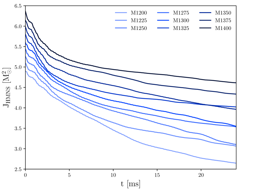
Figure 1: Angular momentum of the merger remnant as a function of time in the post-merger phase from the simulations of [42, 43] for the case of the APR4 EOS. The origin of the time axis is the instant of merger. Different curves correspond to different initial gravitational masses of the NSs.

III Definition of the toy model

The main quantity that we are interested in modeling from the aforementioned simulations is the evolution of the angular momentum of the merger remnant, denoted as $J_{\rm HMNS}$. This is computed from the simulation data as the difference between the Arnowitt-Deser-Misner (ADM) angular momentum of the system, $J_{\rm ADM}$ (i.e., the initial value of the angular momentum), and the angular momentum emitted in GW, $J_{\rm GW}$, i.e., ${J_{\rm HMNS}=J_{\rm ADM}-J_{\rm GW}}$ (see e.g., [61] for a definition of these quantities). Since we are only interested in the post-merger behavior, we define the time of merger $t_{\rm merger}$ as the time at which the GW strain amplitude reaches its first maximum [43] and set it from now forth as the origin of our time axis, i.e., $t_{\rm merger}=0$.

Figure 2: Schematic representation of the post-merger angular momentum evolution as a function of time as predicted by the model defined in section Sec. III.

As an example of the post-merger angular momentum behavior, Fig. 1 shows $J_{\rm HMNS}$ as a function of time, as computed from the simulations of [42, 43], employing the APR4 EOS. Note that all the curves can be roughly described by two lines of constant slope, the first transitioning into the second at approximately 5 ms after merger. This behavior is schematically shown in the simple graphical depiction of Fig. 2, which also illustrates the main quantities discussed in the following paragraphs. In particular, one can follow the angular momentum evolution starting from the merger, undergoing the transient phase where the stellar cores oscillates, and finally reaching the rotating bar configuration, which lasts until the angular momentum is sufficiently large to compensate the gravitational pressure. A detailed definition of all the quantities involved in these phases is the goal of this section.

First of all, it is necessary to define the HMNS angular momentum at merger, i.e., $J_{\rm merger}=J_{\rm HMNS}(t=0)$. We find that the dimensionless quantity $J_{\rm merger}/R^{2}_{\rm NS}$, where $R_{\rm NS}$ is the progenitor NS radius, can be fit by a simple linear universal (i.e., EOS independent) relation in terms of the compactness of the NSs, $C_{\rm NS}$, namely

$$\frac{J_{\rm merger}}{R^{2}_{\rm NS}}=a_{1}C_{\rm NS}+a_{2}\,,$$ (1)

where the coefficients have values $a_{1}=0.8765\pm 0.0051$ and ${a_{2}=-(5.209\pm 0.077)\times 10^{-2}}$. In Eq. (1) and following the errors correspond to $1\sigma$ uncertainties. This universal relation is shown in Fig. 3 along with the simulation data.

After having determined the initial value of the angular momentum evolution in the post merger phase in Eq. (1), we need to model the subsequent evolution of $J_{\rm HMNS}$. As mentioned above, to this end we employ the model first proposed in [42], which we summarize in the following paragraphs, and extend it to later times.

In the toy model, the HMNS is modeled, in a first phase immediately after merger, by a very simple mechanical system consisting of two spheres placed over a rotating disk and connected by a spring (compare to Fig. 4.). After approximately 5 ms, a second phase begins where the HMNS is modeled as a rigid rotating bar.

We focus at first on the transient phase. Consider a mechanical system composed of a disk of mass $M_{\rm disk}$ and radius $R_{\rm disk}$ rotating at a given angular velocity $\Omega_{\rm disk}$ with corresponding rotation frequency $f_{\rm disk}$. Two spheres are placed on the disk, each of mass $M_{\rm sphere}$, connected to each other by a spring and free to oscillate along their separation vector.

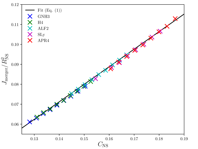
Figure 3: Angular momentum at the time of merger normalized by the square of the progenitor NS radius as a function of the compactness of the initial NSs.

Because of angular momentum conservation the angular velocity of the system increases when the two spheres are closer, and slows down when they move apart. The rotation frequency of the system is therefore bound between a minimum value, $f_{\rm disk,1}$, and a maximum one, $f_{\rm disk,3}$. Dissipative processes (i.e., the friction of the spring between the sphere in this approximation) damp the oscillations in the spheres’ separation on a timescale of a few milliseconds towards a constant rotation frequency value $f_{\rm disk,2}\simeq(f_{\rm disk,1}+f_{\rm disk,3})/2$, which remains nearly unchanged until the collapse time. We call the sum of the spheres’ masses $M_{\rm core}=2M_{\rm sphere}$, and the separation between the two $L_{\rm core}$. The spring has an elastic constant $k$ such that $\Omega_{\rm disk}\approx\sqrt{k/M_{\rm core}}$.

With the definitions above, the equation describing the radial displacement $d(t)$ of a sphere with respect to its position at rest takes the form [42]

$$\ddot{d}+\frac{4kd}{M_{\rm core}}-\Omega_{\rm disk}^{2}d+\frac{2b(\dot{d}-v_{0})}{M_{\rm core}}=0\,,$$ (2)

where the angular velocity $\Omega_{\rm disk}$ is a time-dependent quantity computed as

$$\Omega_{\rm disk}=\frac{J_{\rm merger}/M_{\rm core}}{d^{2}+M_{\rm disk}R^{2}_{\rm disk}/(2M_{\rm core})}\,,$$ (3)

$b$ is a damping constant accounting for the dissipative processes mentioned above, $v_{0}$ is the speed at plunge (i.e., the speed at which the oscillations of the two cores begin), and overdots indicate differentiation with respect to time.

Figure 4: Schematic drawing of the model system for the first phase of the post-merger evolution of the merger remnant.

Assuming without loss of generality the rotation of the disk to take place in the $(x,y)$ plane, the non-zero components of the quadrupole-moment tensor of the model system take the form

$$Q^{\rm disk}_{xx}=\frac{M_{\rm core}d^{2}}{2}[1+\cos(2\Omega_{\rm disk}t)]$$ (4a)

$$Q^{\rm disk}_{yy}=\frac{M_{\rm core}d^{2}}{2}[1-\cos(2\Omega_{\rm disk}t)]$$ (4b)

$$Q^{\rm disk}_{xy}=\frac{M_{\rm core}d^{2}}{2}\sin(2\Omega_{\rm disk}t)=Q^{\rm disk}_{yx}\,.$$ (4c)

From the quadrupole formula, the angular momentum lost by the system per unit time (in the $z$-direction, given our choice of orientation of the system) is [62]

$$\frac{dJ}{dt}=\frac{2}{5}\epsilon^{zkl}\langle\ddot{Q}_{ka}\dddot{Q}_{la}\rangle\,,$$ (5)

where $\epsilon^{ikl}$ is the 3-dimensional Levi-Civita symbol, and the angled brackets indicate a time average over several rotation periods. Therefore the evolution of the angular momentum as function of time simply reads

$$J_{\rm HMNS}(t)=J_{\rm merger}-t\left(\frac{dJ}{dt}\right)_{\rm cores}\,,$$ (6)

i.e., the angular momentum decreases linearly with a slope constant over time.

In the second phase of the post-merger evolution, the radial oscillations of the remnant star cores stop and we can approximate the system with a rotating bar of fixed length. The frequency of rotation of the bar is $f_{\rm disk,2}$, i.e., the frequency towards which the oscillations of the previous phase tend to. We assume the mass of the bar to be equal to $M_{\rm core}$, i.e., the sum of the two star cores, and denote its length by $L_{\rm bar}$. The bar is spinning with constant angular velocity $\Omega_{2}=2\pi f_{\rm disk,2}$ around the $z$-axis (see e.g., Sec. IV.3 for additional discussions on this assumption). The angular velocity $\Omega_{2}$ corresponds to the value of $\Omega_{\rm disk}(t)$ in Eq. (3) for late times.

It is then possible to compute the components of the quadrupole tensor of the system yielding

$$Q^{\rm bar}_{xx}=\frac{M_{\rm core}L^{2}_{\rm bar}}{24}[1+\cos(2\Omega_{2}t)]$$ (7a)

$$Q^{\rm bar}_{yy}=\frac{M_{\rm core}L^{2}_{\rm bar}}{24}[1-\cos(2\Omega_{2}t)]$$ (7b)

$$Q^{\rm bar}_{xy}=\frac{M_{\rm core}L^{2}_{\rm bar}}{24}\sin(2\Omega_{2}t)=Q^{\rm bar}_{yx}\,.$$ (7c)

Proceeding analogously to the discussion above, we finally obtain the expression of the angular momentum loss,

$$\left(\frac{dJ}{dt}\right)_{\rm bar}=\frac{2}{45}M^{2}_{\rm core}L^{4}_{\rm bar}\Omega^{5}_{2}\,.$$ (8)

Combining this result with that of the first phase according to Eq. (5), we can express the evolution of the angular momentum in the whole post-merger phase as a linear decrease in time with a piecewise constant slope:

$$J_{\rm HMNS}(t)=\begin{cases}J_{\rm merger}-t\left(\frac{dJ}{dt}\right)_{\rm cores}&\text{ for }t\leq t_{\rm bar}\\ J_{\rm bar}-t\left(\frac{dJ}{dt}\right)_{\rm bar}&\text{ for }t>t_{\rm bar}\\ \end{cases}$$ (9)

where $t_{\rm bar}$ defines the time of change from the oscillating cores phase to the bar phase, and $J_{\rm bar}=J_{\rm HMNS}(t_{\rm bar})$. The evolution profile of the remnant angular momentum is illustrated in Fig. 2.

The last missing piece of the model is a criterion which defines the time of collapse of the merger remnant. Although a possible definition of this quantity has already been proposed in the literature in relation to the maximum bulk mass of the stable TOV solution [30] (see in particular Fig. 14 therein), in this work we will focus on the angular momentum evolution. In fact, since HMNS are supported against collapse by differential rotation, the loss of a sufficient fraction of the angular momentum present at merger should trigger the collapse. In order to estimate the value of said fraction, we looked at the 8 cases (out of the 42 models considered in [42, 43]) in which the HMNS collapsed during the simulation time, thereby providing a value both for the time of collapse, $t_{\rm coll}$, and the corresponding value of the angular momentum, $J_{\rm coll}$, for those combinations of masses and EOS.

In order to make full use of our limited sample of points, it can be very useful to analyze the ratio ${\epsilon_{\rm coll}=J_{\rm coll}/J_{\rm merger}}$ instead of $J_{\rm coll}$ alone. If we consider $\epsilon_{\rm coll}$ depending exclusively on the dimensionless quantity $\tilde{M}=M_{\rm NS}/M_{\rm TOV}$, one can intuitively imagine that for the most massive configurations, i.e., for $\tilde{M}=1$, the collapse into a black hole (BH) happens promptly, so that the loss of angular momentum is minimal, i.e., $\epsilon_{\rm coll}\approx 1$ (see e.g., [63] for additional discussions on the prompt BH formation from BNSs). Similarly, for the less massive binaries, the post-merger remnant can reach a stable configuration so that $\epsilon_{\rm coll}=0$. As a conservative estimate of the lower limit of the NSs masses, we select the minimum mass of the observed NS mass distribution reported in [64], i.e., $M_{\rm min}\approx 1.1$ $\text{M}_{\odot}$. Recalling that all EOSs considered within this work have a TOV mass in the range $2.0-2.2~{}\text{M}_{\odot}$, we obtain an approximate value for $\tilde{M}=M_{\rm min}/M_{\rm TOV}$ of 0.5 for $\epsilon_{\rm coll}=0$.

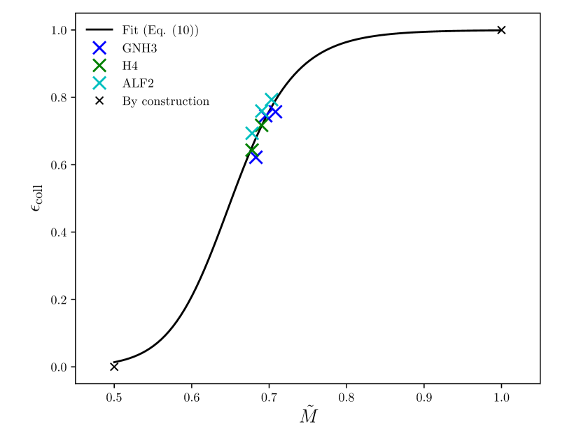
Figure 5: Ratio of the angular momenta at collapse and merger time, ${\epsilon_{\rm coll}=J_{\rm coll}/J_{\rm merger}}$, as a function of the dimensionless mass of the progenitor NSs, $\tilde{M}=M_{\rm NS}/M_{\rm TOV}$.

We show the complete sample of 10 points (8 data points plus the 2 limiting values) for $\epsilon_{\rm coll}$ as function of $\tilde{M}$ in Fig. 5. It can be seen that the data suggests a $\tanh$-like behavior, which tends to 0 for low values of $\tilde{M}$, has a step-like growth around a given value $b_{1}$ (with width $b_{2}$), and converges to 1 for high values of $\tilde{M}$. Concretely we can express the expectations stated above with the following functional relation

$$\epsilon_{\rm coll}=\frac{1}{2}\left[1+\tanh\left(\frac{\log_{10}\tilde{M}-\log_{10}b_{1})}{b_{2}}\right)\right]\,.$$ (10)

$b_{i}$ are two free parameters determined by fitting the data points and which read ${b_{1}=0.6518\pm 0.0081}$ and ${b_{2}=(5.4\pm 1.2)\times 10^{-2}}$. The relation expressed in Eq. (10) is plotted in Fig. 5 together with the considered data and shows an easily understandable physical meaning. Firstly, the extension of the flat plateau at high masses (for $M_{\rm NS}>0.8M_{\rm TOV}$), where the fitting function is nearly equal to unity, can be interpreted as a formal definition of the correlation between prompt collapse and the mass of the progenitor NSs. Conversely, if the progenitor NSs are less massive than roughly 55% of the TOV mass, the post-merger object can be considered stable.

We remark, however, that the quality of the fit is substantially mitigated by the lack of available data points. Testing the precise form of the behavior followed by the curve and the derived conclusions will only be possible with future dedicated numerical simulations.

IV Testing the validity of the model

Now that the physical framework of our model has been defined, we turn our attention to the numerical evaluation of its free parameters. For the model presented in the preceding Sec. III, we need to find for every BNS simulation the values of its parameters. After fixing the value of the free parameters $a_{i}$ and $b_{i}$ in the phenomenological fit functions (1) and (10), respectively, to their best-fit values, only the parameters of the toy model describing the evolution of the angular momentum, i.e., $M_{\rm core}$, $M_{\rm disk}$, $R_{\rm disk}$, $k$, $b$, $v_{0}$, $t_{\rm bar}$ and $L_{\rm bar}$ (see Eq. (9)), remain to be determined.

Assuming no mass loss during the inspiral and negligible mass loss in the post-merger phase (the total value of the mass ejected in BNS merger being of the order of $10^{-2}-10^{-3}$ $\text{M}_{\odot}$, see e.g., [65]), the sum of the mass of the disk and that of the cores has to be equal to the initial total mass of the system, i.e., $M_{\rm tot}=M_{\rm core}+M_{\rm disk}$, allowing us to write

$$\frac{M_{\rm core}}{M_{\rm tot}}+\frac{M_{\rm disk}}{M_{\rm tot}}=\mu_{\rm core}+\mu_{\rm disk}=1\,.$$ (11)

We can therefore consider a single parameter, e.g., $\mu_{\rm disk}~{}\in~{}[0,1]$, in place of both $M_{\rm core}$ and $M_{\rm disk}$. Furthermore, we do not vary $R_{\rm disk}$ and $L_{\rm bar}$ directly but rather work with their dimensionless equivalent ${\rho_{\rm disk}=R_{\rm disk}/R_{\rm NS}}$ and $\lambda_{\rm bar}=L_{\rm bar}/R_{\rm NS}$. This reduces the set of parameters to 7: $\mu_{\rm disk}$, $\rho_{\rm disk}$, $k$, $b$, $v_{0}$, $t_{\rm bar}$ and $\lambda_{\rm bar}$.

To define these parameters for each EOS, we employ a genetic algorithm (GA). This method relies on the minimization of the difference between a quantity predicted by the model, in our case the evolution of the angular momentum, and the corresponding reference value, in our case the results from the simulations of [42, 43].

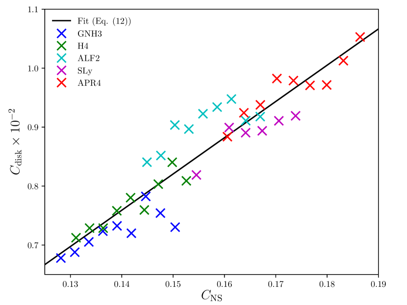
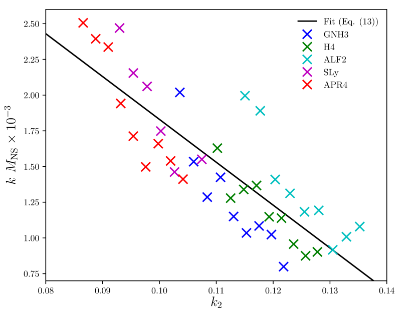
Figure 6: Left panel: Compactness of the disk $C_{\rm disk}$ as function of the initial compactness of the NSs $C_{\rm NS}$. Crosses are simulation data (color coded based on the model EOS), while the black line is the fit of Eq. (12). Right panel: Dimensionless elastic constant $kM_{\rm NS}$ as function of the initial dimensionless Love number $k_{2}$. Crosses are simulation data (color coded based on the model EOS), while the black line is the fit of Eq. (13).

Furthermore, a GA also allows to set additional constraints that have to be fulfilled in order for the algorithm to accept the fitness of a parameter set. This feature becomes particularly useful in our analysis. In fact, by fitting the evolution of the angular momentum with Eq. (9) alone, we would have more free parameters than degrees of freedom (DOFs): in Eq. (9) we have three DOFs ($(dJ/dt)_{\rm cores}$, $J_{\rm bar}$ and $(dJ/dt)_{\rm bar}$) while in the previous paragraph we listed 7 free parameters. Therefore, in order be able to uniquely define each parameter of the model, we need to introduce an additional independent prediction of the model that we can test against the reference at the same time. We choose these constraints to be the values $f_{1}$ and $f_{2}$ of the PSD.

For a more formal definition of the optimization problem, its application to our analysis and the table of the resulting best-fits, Tab. 1, see App. A. There, we also show how the dimensionless disk radius $\rho_{\rm disk}$ and the damping constant $b$ can be fixed to the universal values of $3.5$ and $0.005$, respectively. In this way, one can effectively reduce the number of free parameters to 5: $\mu_{\rm disk}$, $k$, $v_{0}$, $t_{\rm bar}$ and $\lambda_{\rm bar}$.

With both the mathematical and the numerical setup ready, we can apply our procedure to all 42 cases considered within this work. Overall, the mean value of $\tilde{\chi}^{2}$ (defined as in Eq. (15)) that we achieve across the models is $\approx$ 1.44 $\times 10^{-4}$, while the frequencies $f_{1}$ and $f_{2}$ are recovered with an approximate deviation from the values of [42, 43] of 3.1% and 2.8%, respectively.

This level of accuracy is per se already remarkable. It systematically shows for the first time that a mechanical toy model such as the one described in Sec. III can in principle precisely predict the evolution of the angular momentum during the whole post-merger evolution together with other fundamental spectral quantities. In the following paragraphs we further investigate the solidity of the results with different approaches.

IV.1 Universal behavior of the GA results

As a first test of the validity of the GA results, one can look for universal behaviors of the fitted quantities. In fact, these are expected since post-merger quantities, such as the compactness of the cores and the elastic constant, can intuitively be related to characteristics of the progenitor NSs, such as the initial compactness and deformability, respectively. Eventual positive relations found using the GA best-fit values would be a very strong confirmation of the fact that the GA results are not just sourced by degeneracies in the fitting procedure, but have a deeper physical meaning.

The first example we consider is the already mentioned case of the correlation between the compactness of the cores and of the progenitor NSs. Recalling that the radius of the disk has been fixed at the value of 3.5$R_{\rm NS}$ and using the values of $\mu_{\rm disk}$ resulting from the GA, it is possible to compute the disk compactness $C_{\rm disk}$. We find that this can be expressed as function of the initial compactness of the NSs by the linear relation

$$C_{\rm disk}=c_{1}C_{\rm NS}+c_{2}\,,$$ (12)

with the free parameters ${c_{1}=(6.15\pm 0.37)\times 10^{-2}}$ and ${c_{2}=-(1.02\pm 0.34)\times 10^{-3}}$. Eq. (12) is shown in the left panel of Fig. 6 together with the GA best-fits. Using this relation, $\mu_{\rm disk}$ becomes a function of $C_{\rm disk}$ and $R_{\rm disk}$ and the sole knowledge of $M_{\rm NS}$ and $R_{\rm NS}$ determines the values of $\mu_{\rm disk}$, $\mu_{\rm core}$ and $\rho_{\rm disk}$.

In the right panel of Fig. 6, we show the values of the dimensionless elastic constants $kM_{\rm NS}$ as a function of the $\ell=2$ dimensionless tidal Love number $k_{2}$ at infinite separation (see e.g., [43] for more details). Not surprisingly, the parameter that controls the strength of the interaction between the stars in our model is actually correlated with their tidal deformability. We find that the data can in fact be fitted with the following relation

$$kM_{\rm NS}=d_{1}k_{2}+d_{2}\,,$$ (13)

with the free parameters ${d_{1}=-(2.96\pm 0.30)\times 10^{-2}}$ and ${d_{2}=(4.76\pm 0.34)\times 10^{-3}}$.

As a remark, note that our goal in finding universal relations linking the fitted quantities to the initial conditions of the system is only to validate the robustness of the model and of the GA results. They are not made part of the post-merger model in order to reduce its number of free parameters. We leave such a development for a future investigation.

For $v_{0}$, $t_{\rm bar}$ and $\lambda_{\rm bar}$ a clear universal relation could not be found. However, even these parameters can be used to support the validity of our model. Indeed, taking as values the average of the GA results over all configurations, i.e., $v_{0}=0.115$, $t_{\rm bar}=4.83$ ms and $\lambda_{\rm bar}=4.18$, some useful consistency checks can be proposed. For instance, the mean value for $t_{\rm bar}$ corresponds to the expectation stated in [42] regarding the validity of the first phase of the toy model, i.e., that it models the first $\sim 5$ ms of the post-merger.

In conclusion, therefore, we can assume that the GA best-fits are consistent with the expected universal behaviors and truly reflect physical quantities.

IV.2 The representative case of GNH3-M1300

In this following discussion, we also want to make sure that our model, together with its best fit parameters, actually has a predictive power and that the latter is not just limited to the angular momentum evolution. Thus, in order to test its accuracy, we focus our attention on the representative case of the simulation GNH3-M1300, shown in Fig. 7. The choice of this particular case is driven by the analysis of the same configuration made in Appendix A of [42]. Specifically, we want to propose a direct comparison of our results to the ones shown in Figs. 18 and 19 of the reference.

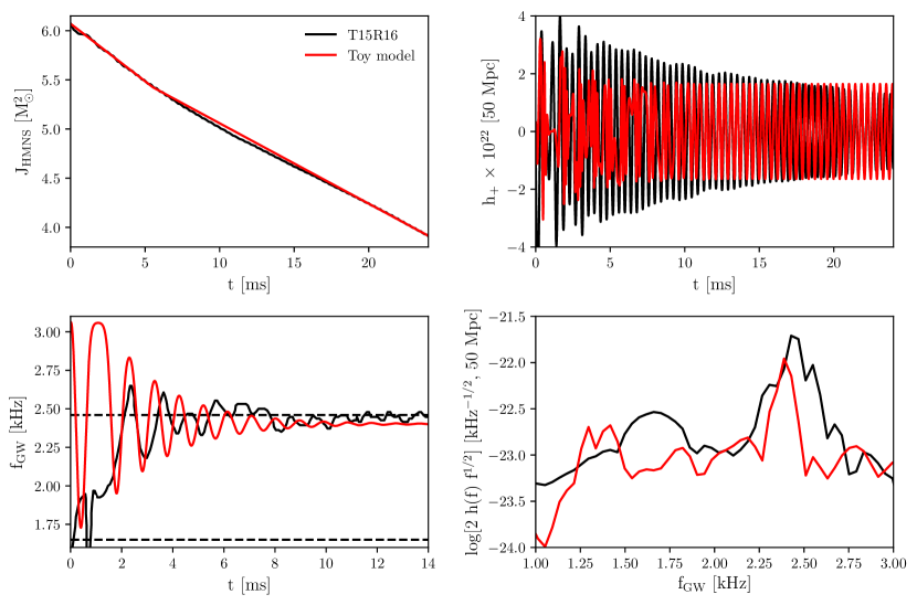
Figure 7: Comparison between (top to bottom, left to right) the post-merger evolution of the angular momentum, the frequency of the GW signal, the GW plus polarization amplitude $h_{+}$ for a source at 50 Mpc and the PSD predicted by our model (red lines) and as computed in the simulations of [42, 43] (black lines, here labeled T15R16 for brevity) for the representative case of GNH3-M1300. The dotted lines in the second panel represent the values of $f_{1}$ and $f_{2}$ as defined in [43].

In Fig. 7 we show the post-merger evolution of the angular momentum in the top left panel, and the frequency of the GWs emitted in the post merger phase as predicted by our model in the bottom left panel. In all panels of Fig. 7, the black lines represent the results from the simulation by [42, 43], while the red lines correspond to the results of our model. Furthermore, the dotted lines in the second panel represent the values of $f_{1}$ and $f_{2}$ as defined in [43].

In both panels, the overlap between the model prediction and the reference is remarkable. This is even more true comparing $f_{\rm GW}$ to the same quantity in Fig. 18 of [42]. The fact alone that such accuracy is possible is non-trivial and should be considered as a strong evidence for the solidity of the toy model.

In order to further test of the robustness of our model, we compute the GW polarization amplitude $h_{+}$ and the PSD of the GW amplitude as defined in [42]. The overlap between the model prediction and reference is plotted in the top and bottom right panels of Fig. 7, respectively. The similarity between the curves is less evident than in the previous cases although still striking, particularly when considering the simplicity of the present model.

These results clearly show that the toy model and the fitting procedure employed within this work to describe the HMNS angular momentum evolution are already very accurate in the prediction of several fundamental quantities over the time range explored by the reference simulations. However, at the same time Fig. 7 also points to the fact that our analysis might still require additional refinements, as for instance the inclusion of more reference quantities in the GA, which could improve the precision of the derived spectral features. This possibility will be addressed in future work.

IV.3 The HMNS lifetime

Since the model accurately reproduces the HMNS evolution within the first 25 ms after the merger, it can be very useful to investigate its validity in terms of the HMNS lifetime. To do so, we calculate the collapse time of all 42 configurations using a linear combination of Eqs. (9) and (10), i.e., with

$$t_{\rm coll}=t_{\rm bar}+\frac{J_{\rm bar}-J_{\rm coll}}{(dJ/dt)_{\rm bar}}$$ (14)

where $J_{\rm bar}=J_{\rm merger}-t_{\rm bar}(dJ/dt)_{\rm toy}$. We then compare the model predictions to the quasi-universal relation found in [66] connecting the HMNS lifetime to the mass of the progenitor NSs.

In Fig. 8, we show the relation of [66] as a black line together with the 1$\sigma$ uncertainty region in gray. The black crosses represent the collapse times of the 8 reference configurations analyzed in [42, 43] that collapsed within the simulation time. Although not explicitly shown in the figure, these data points come with intrinsic uncertainties due to known numerical issues such as the chosen resolution (see e.g., [40, 43, 67] for more details). However, as these errors are particularly difficult to estimate and are not discussed in details in [42, 43], only the single data points are displayed in the figure. The colored crosses represent the model predictions for the different EOSs.

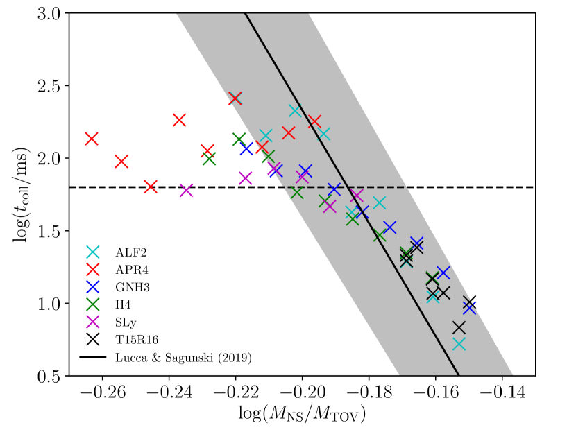
Figure 8: Comparison between the predictions for the HMNS lifetimes calculated using our toy model (colored crosses) and as given in the reference simulations by [42, 43] (black crosses, again labeled T15R16 for shortness), and the relation found in [66] (black line with additional 1$\sigma$ uncertainty region in gray). The horizontal dotted line corresponds to 60 ms.

In the figure it is possible to observe that, although for low values of the collapse times the model predictions are very accurate, they start to diverge from the fit at approximately 60 ms (represented by the horizontal dotted line). There are two main possible explanations for this effect: either Eq. (10) is incorrect in the low mass region (or equivalently for long-living configurations) or there is a late-time softening of the angular momentum decrease, which is not captured by the toy model as it is defined in Sec. III.

We can test the first possibility by setting $J_{\rm coll}$ to zero in Eq. (14), i.e., maximizing the collapse time for all configurations. As it turns out, in this case one only obtains an overall shift of the more massive configurations towards higher collapse times, leaving effectively unchanged the predictions for low-mass binaries.

This points towards the idea that the toy model is currently missing some late-time feature of the angular momentum evolution. Although a detailed modeling of this late-time dynamics will only be possible with the help of extended numerical simulations, in a first approximation one could introduce a third late-time phase in the angular momentum evolution with a reduced emission of GWs.

If we assume that the shape of the HMNS in this phase is still bar-like and that no significant amount of mass is being ejected from the two cores (see e.g., Tab. 1 of [68] for a quantitative overview), according to Eq. (8) there are only two parameters effectively affecting the angular momentum loss rate: the length and the rotation frequency of the bar. As the $f_{2}$ peak in the PSD can often be very sharp (see e.g., Fig. 6 of [43]), we can assume in this approximation that the rotation frequency of the HMNS, which is directly proportional to the frequency of the GW signal, is nearly constant after the transient phase. This conclusion can also be justified in light of recent long-lasting numerical simulations such as the ones performed in [69] (see in particular Fig. 16 therein). This leads to the idea that only the length of the bar may in fact vary over long time ranges.

This fact can be intuitively explained by recalling that as more angular momentum is lost, the rotation velocity of the HMNS becomes less efficient in supporting the star against the gravitational force pulling matter toward the inside. Thus, it leads to an overall compression of the HMNS and therefore a shrinking of its size.

In order to address this limitation of the toy model, we tested straightforward options such as the introduction of a third phase sharply setting on at a time $t_{3}$ and with a reduced value of $L_{\rm bar}$ or a transformation of type ${L_{\rm bar}\to L_{\rm bar}-At}$ in Eqs. (7a)-(7c), where $A$ is a constant driving the rate of change of the bar’s length. While such a modification of the toy model presented here is ultimately desirable to properly capture the late-time evolution of the angular momentum loss, the aforementioned attempts to address it could not fully solve the problem yet. We therefore leave a more in-depth analysis of this aspect to future work, noting also that a proper and systematic exploration of the late-time dynamics of the merger remnant needs data from numerical simulations extending to $\sim 100$ ms after merger (see e.g., [69, 70] for related discussions).

V Conclusions

In the last decade, with the help of a number of fully general relativistic numerical simulations, we achieved an unprecedented understanding of the post-merger evolution of binary NSs. Moreover, the main features of the picture emerging from these simulations have been recently confirmed by the worldwide multimessenger observation of a NS merger, GW170817.

However, the rising complexity necessary to numerically describe these events increases the difficulty in interpreting the physics underlying them. Examples of currently debated aspects of the post-merger evolution involve, for instance, the source of the secondary peaks in the power spectral density and the HMNS lifetime. It is therefore often helpful to simplify the dynamics of the system by means of toy models. In this regard, a particularly useful quantity to track over the whole binary evolution is the angular momentum of the post-merger object. This is because this parameter is tightly connected to key observables, such as the GW emission, and it is also a fundamental ingredient to understand the final stages of the binary evolution, as the star is held against collapse by its high rotational velocity.

In this work, in order to construct a viable toy model for the angular momentum evolution of the HMNS, we first base ourselves on the numerical results of [42, 43] to find a universal relation describing the angular momentum at the time of merger. Then, in order to evaluate the transient phase we employ the toy model defined in [42]. Subsequently, we extend this model to later times by approximating the HMNS as a rotating bar of fixed length. To complete our mathematical setup, we find a second relation connecting the angular momentum of the HMNSs, this time at collapse time, to the initial parameters of the system. For this last step we use once again the results of [42, 43].

Once our extended toy model is defined, to determine the free parameters needed to complete the equations we use a GA. In order to perform a more realistic evaluation of the model, we also include constraints from the evolution of the GW frequency in the GA, which can also be predicted by means of our toy model.

Despite the simplified mathematical setup, several interesting conclusions can be drawn from our results. First of all, we present two original relations (one universal and one quasi-universal) describing the angular momentum at critical moments in the binary evolution, the merger and the collapse.

Furthermore, we systematically show that it is in principle possible to precisely predict the evolution of the angular momentum of a BNS merger remnant as well as many characteristics of its GW signal by means of the aforementioned toy model. Note that, although other models of the post-merger GW signal are available in the literature, such as the one developed by [44, 71], here we follow a different approach. For instance, we do not assume a functional form for the GW signal (which in principle could be arbitrary and not linked to the properties of the merger remnant) and then fit its parameters on numerical data. Instead, we start from a mechanical model of the internal structure of the remnant, which has the advantage of allowing a tighter and more physical connection between the model’s free parameters and the derived quantities. Moreover, the primary goal of our model is to recover the angular momentum evolution, and not the evolution of the GW signal itself, which in our case only becomes a derived quantity.

Given our setup, the fact that extremely accurate fits are possible for every EOS and mass configuration already supports the validity of our model. However, we further investigate the precision and the solidity of our results by suggesting intuitive universal relations that the GA results follow nicely. Moreover, using the same fitting parameters we also derive additional spectral properties, such as the polarization amplitudes and the PSD, and compare them to the reference simulations by [42, 43] for a representative case.

Additionally, we compute the HMNS lifetime for every mass configuration considered within this work. Using the results of [66], we then show that our model is very predictive up to lifetimes roughly in the order of ${60}$ ms, and that there must be a late-time phase in the binary evolution, where the length of the spinning bar is significantly reduced and the loss of angular momentum is even slower than in the quasi-stationary phase.

Finally, however, it is important to underline some limitations of our analysis. First of all, we limited our initial sample to equal-mass binaries and future work will be needed in order to enlarge the progenitor NS mass-ratio range. Secondly, the amount of EOSs considered within this work should also be increased. Other constraints come from the simulations used to produce the initial data. There, effects like fluid viscosity, electromagnetic fields and neutrino transport have been neglected. Also, thermal effects in the fluid are accounted for only approximately via an ideal-gas EOS contribution. Furthermore, we will devote future work to extend the number of constraints as well as the set of minimized functions, e.g., by including the evolution of the energy emitted through GWs.

Appendix A The setup of the genetic algorithm

To find the desired relation linking the evolution of the angular momentum and the initial parameters of the system we set up a fitting procedure as a constrained non-linear optimization problem:

$$\begin{array}[]{ll@{}ll}\text{minimize}&\displaystyle f(\vec{x})&\\ \text{subject to}&\displaystyle g_{j}(\vec{x})\leq 0,&&j=1,...,n\\ &\displaystyle x_{L,i}\leq x_{i}\leq x_{R,i},&&i=1,...,7\,,\end{array}$$

where $f(\vec{x})$ is the objective function (i.e., the function whose minimum corresponds to the optimal parameters’ values), $g_{j}(\vec{x})$ are a set of constraints, $\vec{x}$ is a 7-dimensional vector whose components are the model parameters, e.g., $\vec{x}=\left(\mu_{\rm disk},\rho_{\rm disk},k,b,v_{0},t_{\rm bar},\lambda_{\rm bar}\right)^{T}$, and $\{x_{L,i}$, $x_{R,i}\}$ are lower and upper bounds for the parameters.

As the minimization function $f(\vec{x})$ we choose the least squares $\tilde{\chi}^{2}$:

$$\tilde{\chi}^{2}=\frac{1}{l}\sum_{\rm k=1}^{l}\frac{(J_{\rm HMNS}(t_{\rm k})-J_{\rm data}(t_{\rm k}))^{2}}{J_{\rm data}(t_{\rm k})}\,,$$ (15)

where $J_{\rm HMNS}$ is the angular momentum value predicted by Eq. (9) and $J_{\rm data}$ is the value provided by the simulation data (see Fig. 1). As summarized in Fig. 2, the decrease in $J_{\rm HMNS}(t)$ as predicted by our model consists simply in two linear pieces of constant slope and it is therefore very unlikely that it can accurately describe the transition phase from the oscillating-spheres configuration to the rotating bar one. Acknowledging this limitation we include deviations of the model from the data in the computation of $\tilde{\chi}^{2}$ only over two specific time windows: the first $3$ ms immediately after merger; and the $6$ ms before collapse, or before $t=25$ ms for the simulations in which the collapse was not observed during the simulation time. Therefore the index $k$ in Eq. (15) effectively only runs over the data points within these two time windows.

We include furthermore two constraints based on the GW frequencies $f_{1}$ and $f_{2}$:

$$g_{1} =\frac{f_{\rm 1,ref}-f_{\rm 1,model}(\vec{x})}{f_{\rm 1,ref}}-0.05f_{\rm 1,ref}$$ (16)

$$g_{2} =\frac{f_{\rm 2,ref}-f_{\rm 2,model}(\vec{x})}{f_{\rm 2,ref}}-0.05f_{\rm 2,ref}\,,$$ (17)

where $f_{\rm 1,model}$ and $f_{\rm 2,model}$ are the minimum frequency of the post-merger GW signal and its limit frequency at late times, respectively, as predicted by our model, and $f_{\rm 1,ref}$ and $f_{\rm 2,ref}$ are the corresponding reference values according to the simulations of [42, 43]. The constraint functions are designed to allow for a tolerance of 5% on the deviation of the model frequencies from the reference ones.

An optimization method based on a gradient search would most likely converge to a local minimum of the problem, rather than to the global one. To avoid this behavior the gradient of the 7-dimensional parameter space has to be mapped out with very high precision, which is computationally very expensive and impractical. We have therefore elected to apply a non-gradient based search algorithm. Among this class of algorithms we select a genetic algorithm (GA), as it is known to be very efficient in searching for global minima. The GA we employ is provided by the Python- based package pyOpt [72], of which we make use of the optimizer NSGA2 (Non Sorting Genetic Algorithm II) [73].

Over the course of the generations produced by the GA a given parameter evolves towards its optimal value. Some parameters however have a greater influence on the value of the fitness function then others. Furthermore we observe that some parameters remain nearly constant during the optimization process (i.e., they converge nearly immediately to the optimal value), and that the small variations they experience do not affect significantly the value of $\tilde{\chi}^{2}$. We take advantage of this behavior to further reduce the number of parameters.

EOS	$\displaystyle\frac{\mu_{\textrm{disk}}}{10^{-2}}$	$\displaystyle\frac{k}{10^{-4}}$	$\displaystyle\frac{v_{0}}{10^{-1}}$	$\displaystyle t_{\textrm{bar}}$	$\lambda_{\textrm{bar}}$
ALF2-1200	10.1	9.00	1.12	7.38	3.52
ALF2-1225	10.1	8.23	0.77	5.00	4.14
ALF2-1250	10.5	7.34	0.43	5.32	3.80
ALF2-1275	10.3	9.36	0.84	6.83	3.42
ALF2-1300	10.4	9.10	0.59	4.24	4.73
ALF2-1325	10.3	9.91	0.60	6.30	3.85
ALF2-1350	10.3	10.4	0.84	5.12	4.64
ALF2-1375	9.71	13.7	1.56	4.50	4.31
ALF2-1400	9.62	14.3	1.62	3.97	4.74
APR4-1200	9.63	11.8	1.13	7.37	4.28
APR4-1225	9.88	12.6	1.63	6.11	4.14
APR4-1250	9.83	13.3	1.59	4.11	4.43
APR4-1275	10.1	11.7	0.65	5.46	3.77
APR4-1300	9.88	13.2	0.55	4.25	3.94
APR4-1325	9.62	14.7	0.56	4.18	2.90
APR4-1350	9.45	17.3	0.62	3.79	3.16
APR4-1375	9.67	17.4	0.56	3.86	2.92
APR4-1400	9.88	17.9	0.50	3.99	2.70
GNH3-1200	9.26	6.66	1.34	2.29	5.34
GNH3-1225	9.20	8.36	1.61	1.48	5.00
GNH3-1250	9.24	8.67	1.60	6.10	4.70
GNH3-1275	9.29	8.12	1.15	2.18	5.02
GNH3-1300	9.22	8.85	1.09	5.48	4.97
GNH3-1325	8.88	10.8	1.63	1.59	4.64
GNH3-1350	9.46	9.53	1.46	4.51	5.02
GNH3-1375	8.95	11.2	1.53	6.39	4.60
GNH3-1400	8.50	14.4	1.89	6.08	4.38
H4-1200	9.51	7.52	1.59	2.51	5.34
H4-1225	9.54	7.14	1.13	3.19	4.83
H4-1250	9.35	7.66	1.09	4.92	4.75
H4-1275	9.54	8.93	1.53	4.68	5.01
H4-1300	9.63	8.83	1.05	2.60	4.96
H4-1325	9.20	10.3	1.35	6.45	4.62
H4-1350	9.56	9.92	1.08	5.84	4.85
H4-1375	9.81	9.30	1.02	6.24	5.09
H4-1400	9.28	11.6	1.32	6.11	4.60
SLy-1200	9.27	12.9	2.01	7.38	4.78
SLy-1250	9.78	11.7	1.08	7.36	4.45
SLy-1275	9.49	13.7	1.58	6.03	3.83
SLy-1300	9.34	15.9	1.79	5.68	3.55
SLy-1325	9.34	16.3	1.42	3.17	3.97
SLy-1350	9.25	18.3	1.39	5.25	3.29

Table 1: Genetic algorithm results for the set of 5 parameters. The various columns denote the EOS and the average gravitational mass $M_{\textrm{NS}}$ at infinite separation in $M_{\odot}/10^{-3}$ (”EOS-M${}_{\textrm{NS}}$”), the dimensionless parameter $\mu_{\textrm{disk}}=M_{\textrm{disk}}/M_{\textrm{tot}}$, the elastic constant $k$ in $M_{\odot}^{-1}$, the speed at plunge $v_{0}$, the time $t_{\textrm{bar}}$ in ms at which the system switches from the oscillating configuration to the non-oscillating one, and the dimensionless factor $\lambda_{\textrm{bar}}=L_{\textrm{bar}}/R_{\textrm{NS}}$.

To quantify how much a given parameter $X$ changes along the generations, we define the quantity ${\Theta=\Delta X/X_{\rm opt}}$, where $\Delta X=|X-X_{\rm opt}|$ and $X_{\rm opt}$ is the optimal value of the parameter, i.e., the one belonging to the fittest combination of parameters. We consider the mean value of $\Theta$ over the whole sample:

$$\bar{\Theta}=\frac{\sum^{N}_{\rm i}\Theta_{\rm i}}{N}\,,$$ (18)

where $N=N_{\rm pop}N_{\rm gen}$, $N_{\rm gen}$ being the total number of generations and $N_{\rm pop}$ the number of population members in each generation. We carry out this analysis for the five representative cases ALF2-M1225, APR4-M1350, GNH3-M1300, H4-M1275 and SLy-M1325.

In all cases we find a value of $\bar{\Theta}<0.05$ for the disk mass parameter $\mu_{\rm disk}$, the disk radius $\rho_{\rm disk}$ and the length of the bar configuration $\lambda_{\rm bar}$. In other words these parameters do not significantly evolve during the course of the optimization process.

To quantify the impact of the changes experienced by these parameters on the value of the fitness function or the constraints accuracy, we vary the optimal value of each of the four aforementioned parameters by its relative variation along the generations, i.e., we set $X_{\rm opt}\to X^{\prime}=X_{\rm opt}+X_{\rm opt}\bar{\Theta}$ and compute the corresponding variation in the fitness function and constraints for the five representative models listed above.

As a representative example, in the case of model GNH3-M1300, this procedure applied to $\mu_{\rm disk}$ and $\rho_{\rm disk}$ results in a variation of $\tilde{\chi}^{2}$ of a factor 100 and 50, respectively, while the frequencies vary by less than 2%. Since $\lambda_{\rm bar}$ is the parameter that influences $(dJ/dt)_{\rm bar}$ the most, varying it leads to an increase of the value of $\tilde{\chi}^{2}$ by a factor 140. Analyzing the impact of the remaining three parameters, we observe that even if the damping constant $b$ has a mean $\bar{\Theta}$ of $\approx$ 8%, this leads to variations of $\tilde{\chi}^{2}$ of a factor 0.5, and of $f_{1}$ and $f_{2}$ of less than 1%.

At this point a second consideration comes into play. Examining Eqs. (2) and (3), it is apparent that quantities such as e.g., $M_{\rm disk}$ and $R_{\rm disk}$ are degenerate, appearing in the equations only through their product. This means that although small variations in $R_{\rm disk}$ can considerably vary $\tilde{\chi}^{2}$, the same holds true for $M_{\rm disk}$ (and $M_{\rm core}$). This consideration does not apply, for instance, to $k$ and $b$ since they are directly multiplied with $d$ or $\dot{d}$.

Summarizing, $\mu_{\rm disk}$ does not vary much during the optimization process but its changes affect the fitness function greatly; $\rho_{\rm disk}$ remains nearly constant and, although its variations may affect $\tilde{\chi}^{2}$, they can also be offset by $\mu_{\rm disk}$ (and $\mu_{\rm core}$); the changes in $b$ do not modify significantly $\tilde{\chi}^{2}$; and varying $\lambda_{\rm bar}$ has a large impact on $\tilde{\chi}^{2}$.

We decided therefor to fix $\rho_{\rm disk}$ and $b$ to the constant values of $3.5$ and $0.005$, respectively, which are roughly the mean values of these parameters for the 5 representative models. The remaining parameters are determined by the GA, for all EOSs and all mass configurations, with $N_{\rm pop}=300$ and $N_{\rm gen}=100$. The GA results are listed in Table 1.

References

- Giacconi et al. [1962] R. Giacconi, H. Gursky, F. R. Paolini, and B. B. Rossi, Evidence for x Rays From Sources Outside the Solar System, Phys. Rev. Lett. 9, 439 (1962).
- Hewish et al. [1968] A. Hewish, S. J. Bell, J. D. H. Pilkington, P. F. Scott, and R. A. Collins, Observation of a Rapidly Pulsating Radio Source, Nature 217, 709 (1968).
- Yakovlev et al. [2013] D. G. Yakovlev, P. Haensel, G. Baym, and C. Pethick, Lev Landau and the concept of neutron stars, Physics-Uspekhi 56, 289 (2013).
- Baym [1982] G. Baym, Neutron stars: the first fifty years, in The Neutron and its Applications (1982).
- Hulse and Taylor [1975] R. A. Hulse and J. H. Taylor, Discovery of a pulsar in a binary system, Astrophysical Journal 195, L51 (1975).
- Eichler et al. [1989] D. Eichler, M. Livio, T. Piran, and D. N. Schramm, Nucleosynthesis, neutrino bursts and gamma-rays from coalescing neutron stars, Nature 340, 126 (1989).
- Narayan et al. [1992] R. Narayan, B. Paczynski, and T. Piran, Gamma-ray bursts as the death throes of massive binary stars, Astrophys. J. Lett. 395, L83 (1992), astro-ph/9204001 .
- [8] LIGO collaboration, A Brief History of LIGO, https://www.ligo.caltech.edu/system/media_files/binaries/313/original/LIGOHistory.pdf, accessed: 2019-10-28.
- [9] Gamma-Ray Astrophysics Team, NSSTC, Fermi GBM, https://gammaray.msfc.nasa.gov/gbm/, accessed: 2019-10-28.
- Abbott et al. [2017a] B. P. Abbott et al. (LIGO Scientific Collaboration and Virgo Collaboration), Multi-messenger Observations of a Binary Neutron Star Merger, Astrophys. J. Lett. 848, L12 (2017a).
- Abbott et al. [2017b] B. P. Abbott et al. (LIGO Scientific Collaboration and Virgo Collaboration), Gravitational Waves and Gamma-Rays from a Binary Neutron Star Merger: GW170817 and GRB 170817A, Astrophys. J. Lett. 848, L13 (2017b), arXiv:1710.05834 [astro-ph.HE] .
- Abbott et al. [2017c] B. P. Abbott et al. (LIGO Scientific Collaboration and Virgo Collaboration), GW170817: Observation of Gravitational Waves from a Binary Neutron Star Inspiral, Phys. Rev. Lett. 119, 161101 (2017c).
- Goldstein et al. [2017] A. Goldstein et al., An Ordinary Short Gamma-Ray Burst with Extraordinary Implications: Fermi-GBM Detection of GRB 170817A, Astrophys. J. Letters 848, L14 (2017), arXiv:1710.05446 [astro-ph.HE] .
- Savchenko et al. [2017] V. Savchenko et al., INTEGRAL Detection of the First Prompt Gamma-Ray Signal Coincident with the Gravitational-wave Event GW170817, Astrophys. J. Letters 848, L15 (2017), arXiv:1710.05449 [astro-ph.HE] .
- Coulter and et al. [2017] D. A. Coulter and et al., Swope Supernova Survey 2017a (SSS17a), the optical counterpart to a gravitational wave source, Science 358, 1556 (2017), arXiv:1710.05452 [astro-ph.HE] .
- Abbott et al. [2017d] B. P. Abbott et al. (LIGO Scientific Collaboration and Virgo Collaboration), Estimating the Contribution of Dynamical Ejecta in the Kilonova Associated with GW170817, Astrophys. J. Lett. 850, L39 (2017d), arXiv:1710.05836 [astro-ph.HE] .
- Rasio and Shapiro [1992] F. A. Rasio and S. L. Shapiro, Hydrodynamical evolution of coalescing binary neutron stars, Astrophys. J. 401, 226 (1992).
- Ruffert and Melia [1994] M. Ruffert and F. Melia, Hydrodynamical 3D Bondi-Hoyle accretion onto the Galactic Center blackhole candidate SGR A*, Astron. Astrophys. 288, L29 (1994).
- Shibata and Uryu [2000] M. Shibata and K. Uryu, Simulation of merging binary neutron stars in full general relativity: case, Phys. Rev. D61, 064001 (2000), arXiv:gr-qc/9911058 [gr-qc] .
- Shibata and Uryū [2001] M. Shibata and K. Uryū, Computation of gravitational waves from inspiraling binary neutron stars in quasiequilibrium circular orbits: Formulation and calibration, Phys. Rev. D 64, 104017 (2001).
- Shibata and Uryu [2002] M. Shibata and K. Uryu, Gravitational waves from the merger of binary neutron stars in a fully general relativistic simulation, Prog. Theor. Phys. 107, 265 (2002), arXiv:gr-qc/0203037 [gr-qc] .
- Font et al. [2002] J. A. Font, T. Goodale, S. Iyer, M. Miller, L. Rezzolla, E. Seidel, N. Stergioulas, W.-M. Suen, and M. Tobias, Three-dimensional numerical general relativistic hydrodynamics. ii. long-term dynamics of single relativistic stars, Phys. Rev. D 65, 084024 (2002).
- Shibata and Taniguchi [2006] M. Shibata and K. Taniguchi, Merger of binary neutron stars to a black hole: disk mass, short gamma-ray bursts, and quasinormal mode ringing, Phys. Rev. D73, 064027 (2006), arXiv:astro-ph/0603145 [astro-ph] .
- Anderson et al. [2008] M. Anderson, E. W. Hirschmann, L. Lehner, S. L. Liebling, P. M. Motl, D. Neilsen, C. Palenzuela, and J. E. Tohline, Simulating binary neutron stars: Dynamics and gravitational waves, Phys. Rev. D77, 024006 (2008), arXiv:0708.2720 [gr-qc] .
- Yamamoto et al. [2008] T. Yamamoto, M. Shibata, and K. Taniguchi, Simulating coalescing compact binaries by a new code SACRA, Phys. Rev. D78, 064054 (2008), arXiv:0806.4007 [gr-qc] .
- Baiotti et al. [2008] L. Baiotti, B. Giacomazzo, and L. Rezzolla, Accurate evolutions of inspiralling neutron-star binaries: Prompt and delayed collapse to a black hole, Phys. Rev. D 78, 084033 (2008), arXiv:0804.0594 [gr-qc] .
- Rezzolla et al. [2010] L. Rezzolla, L. Baiotti, B. Giacomazzo, D. Link, and J. A. Font, Accurate evolutions of unequal-mass neutron-star binaries: properties of the torus and short GRB engines, Class. Quantum Grav. 27, 114105 (2010), arXiv:1001.3074 [gr-qc] .
- Anderson et al. [2008] M. Anderson, E. W. Hirschmann, L. Lehner, S. L. Liebling, P. M. Motl, D. Neilsen, C. Palenzuela, and J. E. Tohline, Magnetized neutron-star mergers and gravitational-wave signals, Phys. Rev. Lett. 100, 191101 (2008), arXiv:0801.4387 [gr-qc] .
- Giacomazzo et al. [2011] B. Giacomazzo, L. Rezzolla, and L. Baiotti, Accurate evolutions of inspiralling and magnetized neutron stars: Equal-mass binaries, Phys. Rev. D 83, 044014 (2011), arXiv:1009.2468 [gr-qc] .
- Ciolfi et al. [2017] R. Ciolfi, W. Kastaun, B. Giacomazzo, A. Endrizzi, D. M. Siegel, and R. Perna, General relativistic magnetohydrodynamic simulations of binary neutron star mergers forming a long-lived neutron star, Phys. Rev. D 95, 063016 (2017), arXiv:1701.08738 [astro-ph.HE] .
- Kaplan et al. [2014] J. D. Kaplan, C. D. Ott, E. P. O’Connor, K. Kiuchi, L. Roberts, and M. Duez, The influence of thermal pressure on equilibrium models of hypermassive neutron star merger remnants, Astrophys. J. 790, 19 (2014), arXiv:1306.4034 [astro-ph.HE] .
- Endrizzi et al. [2020] A. Endrizzi, A. Perego, F. M. Fabbri, L. Branca, D. Radice, S. Bernuzzi, B. Giacomazzo, F. Pederiva, and A. Lovato, Thermodynamics conditions of matter in the neutrino decoupling region during neutron star mergers, Eur. Phys. J. A 56, 15 (2020), arXiv:1908.04952 [astro-ph.HE] .
- Kastaun and Galeazzi [2015] W. Kastaun and F. Galeazzi, Properties of hypermassive neutron stars formed in mergers of spinning binaries, Phys. Rev. D 91, 064027 (2015), arXiv:1411.7975 [gr-qc] .
- Bernuzzi et al. [2016] S. Bernuzzi, D. Radice, C. D. Ott, L. F. Roberts, P. Moesta, and F. Galeazzi, How Loud Are Neutron Star Mergers?, Phys. Rev. D 94, 024023 (2016), arXiv:1512.06397 [gr-qc] .
- Shibata and Kiuchi [2017] M. Shibata and K. Kiuchi, Gravitational waves from remnant massive neutron stars of binary neutron star merger: Viscous hydrodynamics effects, Phys. Rev. D 95, 123003 (2017), arXiv:1705.06142 [astro-ph.HE] .
- Chaurasia et al. [2018] S. V. Chaurasia, T. Dietrich, N. K. Johnson-McDaniel, M. Ujevic, W. Tichy, and B. Brügmann, Gravitational waves and mass ejecta from binary neutron star mergers: Effect of large eccentricities, (2018), arXiv:1807.06857 [gr-qc] .
- Stergioulas et al. [2011] N. Stergioulas, A. Bauswein, K. Zagkouris, and H.-T. Janka, Gravitational waves and non-axisymmetric oscillation modes in mergers of compact object binaries, Mon. Not. R. Astron. Soc. 418, 427 (2011), arXiv:1105.0368 [gr-qc] .
- Bauswein and Janka [2012] A. Bauswein and H.-T. Janka, Measuring Neutron-Star Properties via Gravitational Waves from Neutron-Star Mergers, Phys. Rev. Lett. 108, 011101 (2012), arXiv:1106.1616 [astro-ph.SR] .
- Bauswein et al. [2012] A. Bauswein, H.-T. Janka, K. Hebeler, and A. Schwenk, Equation-of-state dependence of the gravitational-wave signal from the ring-down phase of neutron-star mergers, Phys. Rev. D 86, 063001 (2012), arXiv:1204.1888 [astro-ph.SR] .
- Hotokezaka et al. [2013] K. Hotokezaka, K. Kiuchi, K. Kyutoku, T. Muranushi, Y.-i. Sekiguchi, M. Shibata, and K. Taniguchi, Remnant massive neutron stars of binary neutron star mergers: Evolution process and gravitational waveform, Phys. Rev. D 88, 044026 (2013), arXiv:1307.5888 [astro-ph.HE] .
- Bauswein et al. [2014] A. Bauswein, N. Stergioulas, and H.-T. Janka, Revealing the high-density equation of state through binary neutron star mergers, Phys. Rev. D 90, 023002 (2014), arXiv:1403.5301 [astro-ph.SR] .
- Takami et al. [2015] K. Takami, L. Rezzolla, and L. Baiotti, Spectral properties of the post-merger gravitational-wave signal from binary neutron stars, Phys. Rev. D 91, 064001 (2015), arXiv:1412.3240 [gr-qc] .
- Rezzolla and Takami [2016] L. Rezzolla and K. Takami, Gravitational-wave signal from binary neutron stars: A systematic analysis of the spectral properties, Phys. Rev. D 93, 124051 (2016), arXiv:1604.00246 [gr-qc] .
- Bernuzzi et al. [2015] S. Bernuzzi, T. Dietrich, and A. Nagar, Modeling the complete gravitational wave spectrum of neutron star mergers, Phys. Rev. Lett. 115, 091101 (2015), arXiv:1504.01764 [gr-qc] .
- Bauswein and Stergioulas [2015] A. Bauswein and N. Stergioulas, Unified picture of the post-merger dynamics and gravitational wave emission in neutron star mergers, Phys. Rev. D91, 124056 (2015), arXiv:1502.03176 [astro-ph.SR] .
- Nakamura et al. [1987] T. Nakamura, K. Oohara, and Y. Kojima, General Relativistic Collapse to Black Holes and Gravitational Waves from Black Holes, Progress of Theoretical Physics Supplement 90, 1 (1987).
- Shibata and Nakamura [1995] M. Shibata and T. Nakamura, Evolution of three-dimensional gravitational waves: Harmonic slicing case, Phys. Rev. D 52, 5428 (1995).
- Baumgarte and Shapiro [1999] T. W. Baumgarte and S. L. Shapiro, Numerical integration of Einstein’s field equations, Phys. Rev. D 59, 024007 (1999), gr-qc/9810065 .
- Brown [2009] D. J. Brown, Covariant formulations of Baumgarte, Shapiro, Shibata, and Nakamura and the standard gauge, Phys. Rev. D 79, 104029 (2009).
- Harten et al. [1983] A. Harten, P. D. Lax, and B. van Leer, On upstream differencing and godunov-type schemes for hyperbolic conservation laws, SIAM Rev. 25, 35 (1983).
- Colella and Woodward [1984] P. Colella and P. R. Woodward, The piecewise parabolic method (ppm) for gas-dynamical simulations, Journal of Computational Physics 54, 174 (1984).
- Alford et al. [2005] M. Alford, M. Braby, M. Paris, and S. Reddy, Hybrid stars that masquerade as neutron stars, Astrophys. J. 629, 969 (2005), nucl-th/0411016 .
- Akmal et al. [1998] A. Akmal, V. R. Pandharipande, and D. G. Ravenhall, Equation of state of nucleon matter and neutron star structure, Phys. Rev. C 58, 1804 (1998), arXiv:hep-ph/9804388 .
- Glendenning [1985] N. K. Glendenning, Neutron stars are giant hypernuclei?, Astrophys. J. 293, 470 (1985).
- Glendenning et al. [1992] N. Glendenning, F. Weber, and S. Moszkowski, Neutron stars in the derivative coupling model, Physical Review C 45, 844 (1992).
- Douchin and Haensel [2001] F. Douchin and P. Haensel, A unified equation of state of dense matter and neutron star structure, Astron. Astrophys. 380, 151 (2001), arXiv:astro-ph/0111092 .
- Antoniadis et al. [2013] J. Antoniadis et al., A massive pulsar in a compact relativistic binary, Science 340, 10.1126/science.1233232 (2013).
- Cromartie et al. [2019] H. T. Cromartie et al., Relativistic Shapiro delay measurements of an extremely massive millisecond pulsar, Nature Astron. 4, 72 (2019), arXiv:1904.06759 [astro-ph.HE] .
- Linares et al. [2018] M. Linares, T. Shahbaz, and J. Casares, Peering into the dark side: Magnesium lines establish a massive neutron star in PSR j2215+5135, The Astrophysical Journal 859, 54 (2018).
- Godzieba et al. [2020] D. A. Godzieba, D. Radice, and S. Bernuzzi, On the maximum mass of neutron stars and GW190814, (2020), arXiv:2007.10999 [astro-ph.HE] .
- Baumgarte and Shapiro [2010] T. W. Baumgarte and S. L. Shapiro, Numerical Relativity: Solving Einstein’s Equations on the Computer (Cambridge University Press, Cambridge, UK, 2010).
- Maggiore [2007] M. Maggiore, Gravitational Waves: Volume 1: Theory and Experiments, Gravitational Waves (Oxford University Press, USA, 2007).
- Agathos et al. [2020] M. Agathos, F. Zappa, S. Bernuzzi, A. Perego, M. Breschi, and D. Radice, Inferring Prompt Black-Hole Formation in Neutron Star Mergers from Gravitational-Wave Data, Phys. Rev. D 101, 044006 (2020), arXiv:1908.05442 [gr-qc] .
- Kiziltan et al. [2013] B. Kiziltan, A. Kottas, M. De Yoreo, and S. E. Thorsett, The neutron star mass distribution, Astrophys. J. 778, 66 (2013), arXiv:1309.6635 [astro-ph.SR] .
- Bovard et al. [2017] L. Bovard, D. Martin, F. Guercilena, A. Arcones, L. Rezzolla, and O. Korobkin, On r-process nucleosynthesis from matter ejected in binary neutron star mergers, Phys. Rev. D 96, 124005 (2017), arXiv:1709.09630 [gr-qc] .
- Lucca and Sagunski [2020] M. Lucca and L. Sagunski, The lifetime of binary neutron star merger remnants, JHEAp 27, 33 (2020), arXiv:1909.08631 [astro-ph.HE] .
- Bauswein et al. [2010] A. Bauswein, H.-T. Janka, and R. Oechslin, Testing approximations of thermal effects in neutron star merger simulations, Phys. Rev. D 82, 084043 (2010).
- Shibata and Hotokezaka [2019] M. Shibata and K. Hotokezaka, Merger and mass ejection of neutron star binaries, Annual Review of Nuclear and Particle Science 69, 41 (2019).
- Ciolfi et al. [2019] R. Ciolfi, W. Kastaun, J. V. Kalinani, and B. Giacomazzo, First 100 ms of a long-lived magnetized neutron star formed in a binary neutron star merger, Phys. Rev. D 100, 023005 (2019), arXiv:1904.10222 [astro-ph.HE] .
- Ciolfi [2020] R. Ciolfi, Collimated outflows from long-lived binary neutron star merger remnants, Mon. Not. Roy. Astron. Soc. 495, L66 (2020), arXiv:2001.10241 [astro-ph.HE] .
- Breschi et al. [2019] M. Breschi, S. Bernuzzi, F. Zappa, M. Agathos, A. Perego, D. Radice, and A. Nagar, Kilohertz gravitational waves from binary neutron star remnants: Time-domain model and constraints on extreme matter, Phys. Rev. D 100, 104029 (2019).
- Perez et al. [2012] R. E. Perez, P. W. Jansen, and J. R. Martins, pyopt: a python-based object-oriented framework for nonlinear constrained optimization, Structural and Multidisciplinary Optimization 45, 101 (2012).
- Deb et al. [2002] K. Deb, A. Pratap, S. Agarwal, and T. Meyarivan, A fast and elitist multiobjective genetic algorithm: NSGA-II, IEEE transactions on evolutionary computation 6, 182 (2002).