Filament rotation in the California L1482 cloud

Abstract

We analyze the gas mass distribution, the gas kinematics, and the young stellar objects (YSOs) of the California Molecular Cloud (CMC) L1482 filament. The mean Gaia DR2 YSO distance is 511${}^{+17}_{-16}$ pc. In terms of the gas, the line-mass (M/L) profiles are symmetric scale-free power-laws consistent with cylindrical geometry. We calculate the gravitational potential and field profiles based on these. Our IRAM 30 m multi-tracer position-velocity diagrams highlight twisting and turning structures. We measure the C¹⁸O velocity profile perpendicular to the southern filament ridgeline. The profile is regular, confined (projected $r\lesssim 0.4$ pc), anti-symmetric, and to first order linear, with a break at $r\sim 0.25$ pc. We use a simple solid-body rotation toy model to interpret it. We show that the centripetal force, compared to gravity, increases toward the break; when the ratio of forces approaches unity, the profile turns over, just before the implied filament breakup. The timescales of the inner (outer) gradients are $\sim\,$0.7 (6.0) Myr. The timescales and relative roles of gravity to rotation indicate that the structure is stable, long lived ($\sim$ a few times 6 Myr), and undergoing outside-in evolution. This filament has practically no star formation, a perpendicular Planck plane-of-the-sky (POS) magnetic field morphology, and 2D “zig-zag” morphology, which together with the rotation profile lead to the suggestion that the 3D shape is a ”corkscrew” filament. These results, together with results in other regions, suggest evolution toward higher densities as rotating filaments shed angular momentum. Thus, magnetic fields may be an essential feature of high-mass (M $\sim\,10^{5}$ M_⊙) cloud filament evolution toward cluster formation.

tablenum SIXtablenum

1 Introduction

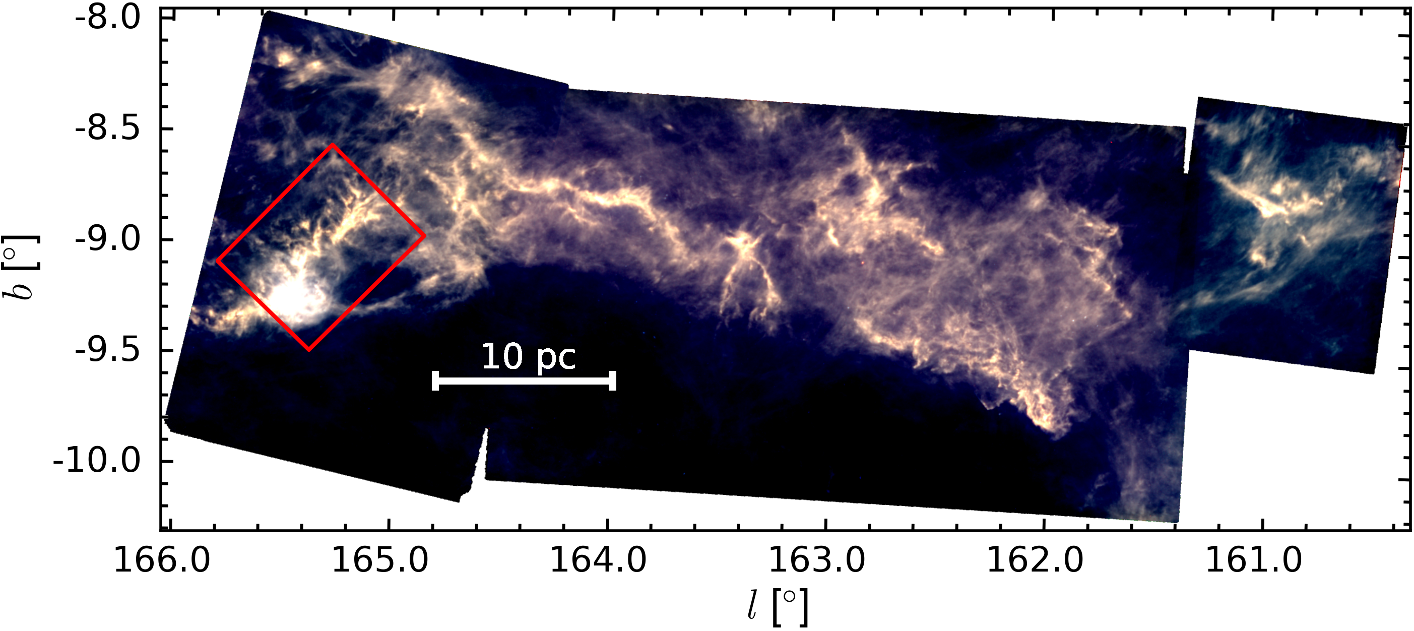
Figure 1: False color Herschel 250 µm (blue), 350 µm (green) and 500 µm (red) image of the California Molecular Cloud (CMC). The red box indicates the approximate portion of the L1482 filament that we analyze in this study. Note the elongated overall structure and the twisting filament spines. In particular, the L1482-South filament, located just to the north of the bright nebulosity produced by the B-star LkH$\alpha$ 101, has a “zig-zag” morphology in the plane of the sky (see text).

Using the ¹²CO (1-0) Dame et al. (2001) data, Miville-Deschênes et al. (2017) show that the mass function of Milky Way clouds peaks near $\rm{M}=10^{5}$ M_⊙. Moreover, most of the molecular mass is contained in high-mass clouds, with 50% of the mass in clouds above $\rm{M}=8.4\times 10^{5}$ M_⊙. Therefore, characterizing the physical properties of spiny star forming filaments in clouds near and above the $\rm{M}=10^{5}$ M_⊙ regime is essential for studying “typical” star formation conditions in our Galaxy.

Meanwhile, the clouds that we can observationally access and scrutinize in extreme detail because of their proximity to us (with distances $\lesssim 500$ pc) typically have significantly lower masses (e.g., Lada et al., 2010). The exceptions to this are the California Molecular Cloud (CMC), Orion A, and Orion B, with masses $\sim\,10^{5}$ M_⊙ (e.g., Megeath et al., 2012; Fischer et al., 2017; Stutz & Kainulainen, 2015; Lada et al., 2009, 2010; Kong et al., 2015). Only recently identified as a separate massive cloud (Lada et al., 2009, and see below), the properties of the CMC dense gas and young stars are significantly less well-characterized than those of the Orion complex. In this paper our primary focus is on the CMC L1482 filament (red box in Figure 1) gas kinematics. We place these gas measurements in the framework required for robust comparison to recent work in Orion A (Stutz & Kainulainen, 2015; Stutz & Gould, 2016; Stutz, 2018; González Lobos & Stutz, 2019) in order to identify possible physical differences that may explain the variations in the observed properties of filaments and their young stars embedded in the gravitational potentials of M$\,\sim\,10^{5}$ M_⊙ clouds.

The CMC, named after its proximity to the California Nebula, was first thought to be part of the Taurus-Auriga complex (e.g., Ungerechts & Thaddeus, 1987; Herbig et al., 2004; Andrews & Wolk, 2008). It was identified as a separate region just over a decade ago by Lada et al. (2009). They found this structure to be at a much larger distance (450 pc) compared to the nearby Taurus-Auriga (150 pc) and Perseus (240 pc) clouds. Lada et al. (2009) noted that the CMC had a similar mass ($\sim$10⁵ M_⊙) and filamentary morphology as Orion A, both being nearby giant molecular clouds (GMCs).

Another important similarity between the two was presented in Tahani et al. (2018). Using Faraday rotation measurements they found that in both the CMC and Orion A the magnetic field flips its line-of-sight direction from one side of the filament to the other. They interpreted these results as a possible indicator of a helical field morphology on larger (cloud) scales (but see below and Tahani et al., 2019, for results in Orion A). However, the exact 3D magnetic field morphology in filaments (including Orion A and the CMC) remains the subject of ongoing debate (e.g. Heiles, 1987, 1997; Matthews & Wilson, 2000; Fiege & Pudritz, 2000a; Falgarone et al., 2001; Hennebelle, 2003; Stutz & Gould, 2016; Schleicher & Stutz, 2018; Reissl et al., 2018a; Tahani et al., 2019; Law et al., 2019, 2020; Reissl et al., 2020). For example, one suggested field morphology that could account for the directional flip in the field is a “bow”-type morphology (see e.g., Inoue et al., 2018; Reissl et al., 2018a; Li & Klein, 2019; Tahani et al., 2019; Gómez et al., 2018). However, the simultaneous detection of filament rotation may be incompatible with this particular field geometry. Thus, the detection of rotation in filaments may present one avenue to distinguish between plausible magnetic field geometries. Moreover, geometries such as helical or toroidal may play a crucial role in filament formation. They prevent expansion, maintaining the filamentary structure, and may also influence the formation of clumps, thereby impacting the star formation within (e.g., Uchida et al., 1991; Fiege & Pudritz, 2000a, b; Contreras et al., 2013; Stutz & Gould, 2016).

More broadly, the detection of rotation in filaments (see e.g. González Lobos & Stutz 2019 for a possible rotational signature in the Orion A Integral Shaped Filament) presents the opportunity to address the angular momentum evolution of massive star and cluster forming systems (e.g. Motte et al., 2018; Kong et al., 2019) in the presence of potentially coherent and smoothly varying magnetic fields. It is also essential to connect large and small scale field properties in star-forming systems, as will be facilitated in the near future with the Prime-cam instrument (Choi et al., 2020) on the Fred Young Submillimeter Telescope (FYST, formerly CCAT-prime; Terry et al., 2019).

In the southeast of the CMC we find L1482, which is one of the most massive filaments in the CMC and contains about 100 YSOs (Lada et al., 2009; Kong et al., 2015; Lada et al., 2017). L1482 hosts the reflection nebula NGC 1579, composed of a young stellar cluster and LkH$\alpha$ 101, the only massive (B type) star in the region (e.g., Herbig et al., 2004; Andrews & Wolk, 2008). Thus the CMC is mostly unaffected by massive-star feedback. By scrutinizing millimeter-wave gas lines, Li et al. (2014) found that the filament structure is most likely coherent, presenting gas velocity gradients that they interpreted as possible inflows feeding the stellar cluster in the northern portion of L1482.

As described above, the CMC and Orion A share several important physical attributes. They both have a similar mass, a similar elongated shape, both contain twisting and winding filaments, and both have comparable magnetic field geometry (along the line-of-sight component) and strengths as probed by Faraday rotation (Tahani et al., 2018). However, despite these similarities, their respective dense gas fraction (Lada et al., 2009) and YSO content are strikingly different. In Orion A there are more than 3000 YSOs (Megeath et al., 2012), whereas the CMC only has about 177 YSOs (Lada et al., 2017). Thus, the CMC is sometimes referred to as a “sleeping giant” (Lada et al., 2017). As this name clearly implies, there is a plausible evolutionary progression between the two clouds. Hence, assuming that the differences can be explained by the CMC being in an earlier evolutionary state at the same mass, the CMC may provide a window into the initial stages of filament evolution and star-cluster formation in GMCs, before reaching the typical yet extreme embedded cluster conditions such as those present in the Orion Nebula Cluster and other bona fide (and hence more distant) protoclusters.

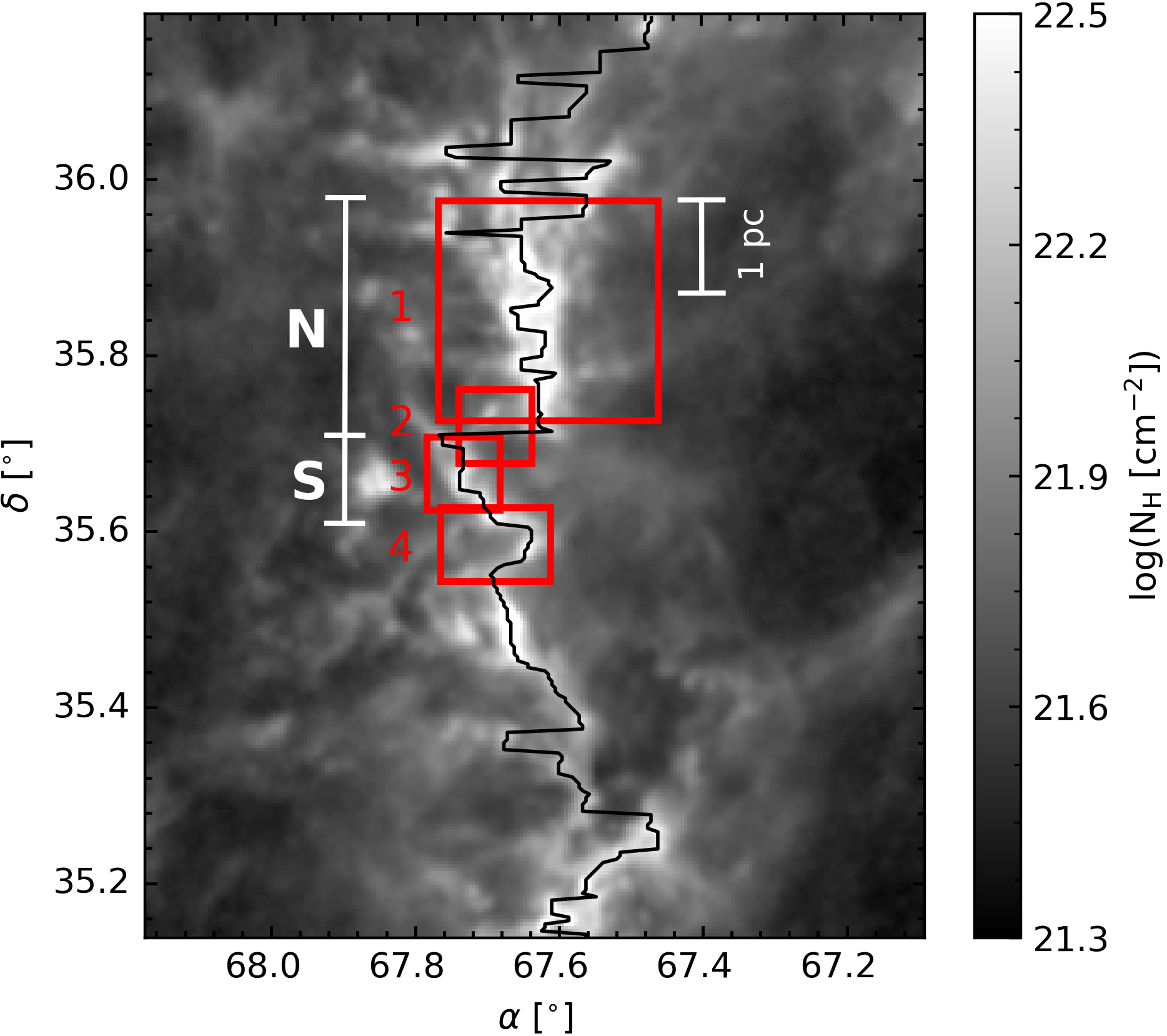
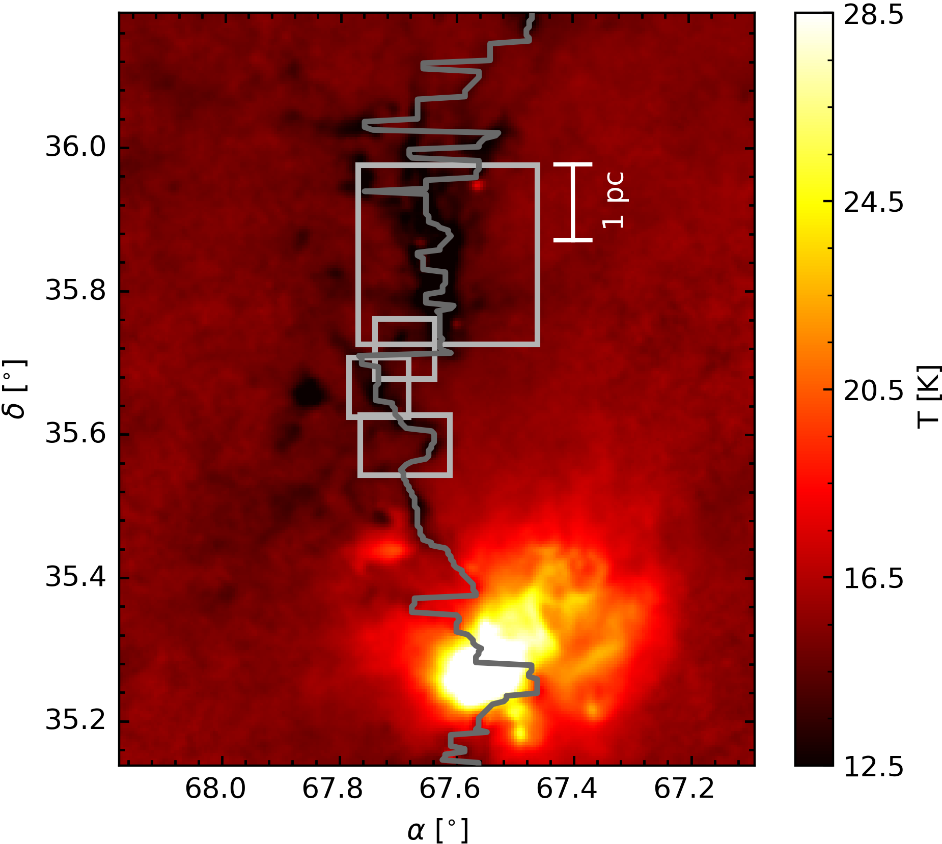
Figure 2: $N_{\rm H}$ (left panel) and temperature (right panel) maps of L1482. The black (left) and grey (right) curves represent the $N_{\rm H}$ ridgeline. The red (left) and grey (right) boxes show the fields observed with the IRAM 30 m radio telescope. In the left panel we indicate the extents of the North ($\delta=35.71\mbox{${}^{\circ}$}\rightarrow 35.98\mbox{${}^{\circ}$}$) and South ($\delta=35.71\mbox{${}^{\circ}$}\rightarrow 35.61\mbox{${}^{\circ}$}$) regions (see § 5.2).

The gas gravitational potential is a crucial parameter in a gas mass dominated system, such as L1482, because it sets the overall dynamics of the system (e.g., Stutz & Gould, 2016). Hence, it forms the basis for any study addressing gas (and stellar) kinematics. In this framework, after presenting the data (§ 2), the first parameter that we must determine is the distance to the system using Gaia (§3). We then estimate the gas gravitational potential and field based on the Herschel and Planck mass map (§ 4). This sets the stage to analyze the gas motions (§ 5) with the goal of characterizing the physical state, specifically highlighting the detection of filament rotation of L1482-South (§ 6). We discuss these results in § 7 and conclude in § 8.

Table 1: Fields observed with IRAM 30m radio telescope.

Field	$\alpha$ [ ∘ ]	$\delta$ [ ∘ ]	size [${}^{\prime\prime}\times^{\prime\prime}$]	Observation Date
1	67.62	35.85	900x900	2018 Jun 21-23
				2018 Jul 16
2	67.69	35.72	300x300	2019 Jan 07
3	67.73	35.67	300x300	2019 Jan 07
4	67.66	35.59	450x300	2019 Jan 07

Note. — Central field coordinates, sizes, and observation dates. See Figure 2.

2 Observations

2.1 Herschel N_H and T maps

We use the publicly available Herschel pipeline data from the Harvey et al. (2013) program. These observations were made using the PACS (Poglitsch et al., 2010) and SPIRE (Griffin et al., 2010) cameras in parallel mode at 160 µm, 250 µm, 350 µm, and 500 µm with beam sizes of 11.8$\arcsec$, 18.2$\arcsec$, 24.9 $\arcsec$, and 36.3$\arcsec$, respectively. Well calibrated flux data are crucial when estimating the column density ($N_{\rm H}$) and temperature (T) maps of a cloud. Here we use the Abreu-Vicente et al. (2017) method to improve the Herschel absolute calibration by using the Planck all-sky dust model and combining the two datasets in Fourier space. We refer the reader to Abreu-Vicente et al. (2017) for more details.

After combining the Herschel and Planck emission maps, we convolve the data to the 500 µm resolution. The convolved images are then re-gridded to the same pixel scale of 14$\arcsec$ ($\sim 0.035$ pc at $D$ = 511 pc, see § 3). We then extract a spectral energy distribution (SED) for each pixel (e.g., Abreu-Vicente et al., 2017; Stutz & Kainulainen, 2015; Launhardt et al., 2013; Stutz et al., 2013, 2010). This SED is fit with the modified black-body (MBB) function of the form:

$$S_{\nu} = \Omega B_{\nu}(\nu,T_{d})(1-\exp^{-{\tau(\nu)}}),$$ (1)

where $\Omega$ is the beam solid angle, $B_{\nu}(T_{\rm d})$ is the Planck function at a dust temperature $T_{\rm d}$, $\tau(\nu)$ is the optical depth at a frequency $\nu$. Here $\tau(\nu)$ = $N_{\rm{H}}m_{\rm{H}}R_{gd}^{-1}\kappa(\nu)$, where $N_{\rm{H}}$ = $2\times N({\rm{H_{2}}})+N(\rm{H})$ is the total hydrogen column density, $m_{\rm{H}}$ is the mass of the hydrogen atom, $\kappa(\nu)$ is the dust opacity, and $R_{gd}$ is the gas-to-dust mass ratio, which is assumed to be 110 (Sodroski et al., 1997). We use the dust opacities from Ossenkopf & Henning (1994) Table 1, column 5. Stutz et al. (2013), Launhardt et al. (2013), and Lombardi et al. (2014) discuss the systematic uncertainties produced by the model. In Figure 2 we show the resulting $N_{\rm H}$ (left panel) and T_d (right panel) maps. We obtain similar maps as those presented in Lada et al. (2017).

Table 2: IRAM 30 m observational parameters.

Tracer	Frequency	HPBW	$\Delta$ V	Backend	Mean Noise ($\sigma_{\rm{rms}}$) [K]
	[GHz]	[”]	[$\rm km\,s^{-1}$]		Field 1	Field 2	Field 3	Field 4
C18O (1-0)	109.782	22.41	0.133	FTS	0.26	0.20	0.20	0.21
N2H+ (1-0)	93.173	26.40	0.157	FTS	0.18	0.12	0.11	0.11
			0.063	VESPA	0.22	0.19	0.18	0.19
HNC(1-0)	90.663	27.13	0.161	FTS	0.19	0.13	0.12	0.13
HCO+ (1-0)	89.188	27.58	0.164	FTS	0.16	0.12	0.12	0.12

Note. — $\Delta$V is the spectral resolution for the respective observation. The last four columns show the noise levels of the data.

2.2 IRAM 30 m molecular line data

We mapped the C¹⁸O (1-0), N₂H⁺ (1-0), HCO⁺ (1-0) and HNC (1-0) molecular lines with the IRAM 30 m telescope with the primary goal of measuring the gas kinematics. We choose C¹⁸O (1-0) (109.782 GHz) as our main tracer with the goal of obtaining measurements of the kinematics of the gas. We also measure N₂H⁺ (1-0) (93.173 GHz), a high-density gas tracer that enables us to observe the spine of the filament (e.g. Caselli et al., 2002; Tafalla et al., 2002; Lippok et al., 2013) when detected. We also include HCO⁺ (1-0) (89.188 GHz) and HNC(1-0) (90.663 GHz) in our observations for mapping filament motions (such as rotation and infall) that may be present in L1482.

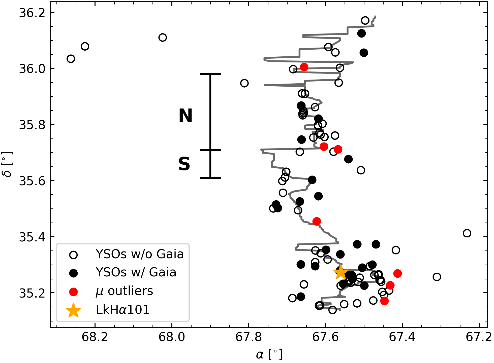
Figure 3: L1482 YSOs from Lada et al. (2017). We show YSOs with Gaia counterparts as filled circles (34 sources); of these, proper motion outliers are indicated in red (7 sources), with the remainder shown in black (see § 3 and Figure 4). YSOs without Gaia counterparts are shown as black open circles (66 sources). We show the B-star LkH$\alpha$ 101 (Herbig et al., 2004) as an orange star. The $N_{\rm H}$ ridgeline is represented as a grey line (see § 4). Vertical black lines indicate the extent of the North (N) and South (S) regions (see § 5.2).

We use the EMIR receiver with the Fast Fourier Transform Spectrometers (FTS) backend for all tracers. For N₂H⁺ the Versatile Spectrometric and Polarimetric Array (VESPA) backend is also used. All the observations were made using On-The-Fly (OTF) mapping mode. The central coordinates, sizes, and observation dates are shown in Table 1. In Table 2 we list the spectral resolution, half power beam width (HPBW) and noise levels of our observations. We combine the fields and reduce the data of all tracers using the CLASS package from GILDAS, software developed by the Institute de Radioastronomie Millimétrique (IRAM). Figure 2 shows the location of our fields of observation. Field 1 covers the northern portion of L1482. Field 2 covers the “transition” zone between the North and the South. Fields 3 and 4 cover the southern portion of L1482.

We also include the ¹³CO (2-1) data from (Kong et al., 2015). These data cover the L1482 filament as a whole and were observed with the 10 m Heinrich Hertz Sub-millimeter Telescope (SMT) on Mount Graham, Arizona. These data have a 35$\arcsec$ beam and a spectral resolution of 0.15 $\rm km\,s^{-1}$. We refer the reader to Kong et al. (2015) for further details.

2.3 Gaia-detected Spitzer Young Stellar Objects

We use Gaia DR2 data (Gaia Collaboration et al., 2018b) crossmatched with the Young Stellar Object (YSO) catalog from Lada et al. (2017). In § 3 we obtain a robust sample for astrometric analysis based on the parameters of Gaia-detected YSOs.

3 Gaia distance to L1482

Most of the YSOs in the Lada et al. (2017) catalog are located in projection on the filament (Figure 3). We therefore infer that most YSOs are embedded in the filament, so that their parallaxes provide a good estimate of the gas filament distance (Stutz et al., 2018).

We begin by constraining the region of our analysis to L1482, or 66.99^∘ $<$ $\alpha$ $<$ 68.27^∘ and 35.13^∘ $<$ $\delta$ $<$ 36.18^∘. We correct the zero-point offset in the Gaia parallaxes based on Zinn et al. (2019). For the crossmatch we set the maximum separation limit to $0.5\arcsec$, since all Gaia-detected sources are within that limit. We accept YSOs with G $\leq\,19$ mag (Lindegren et al., 2018) and positive parallax measurements in the Gaia catalog. Based on these criteria we match 34 out of 100 total YSOs in the area of interest. See Figure 3 for the YSO locations relative to the $N_{\rm H}$ ridgeline and IRAM 30 m observations.

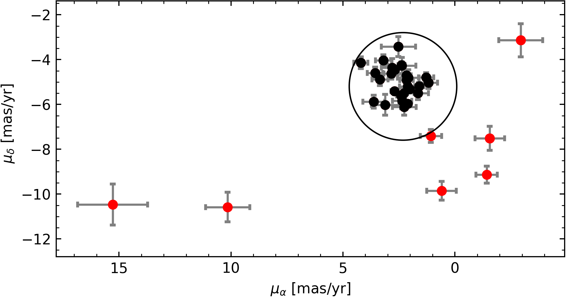
Figure 4: Proper motion ($\mu$) distribution of our sample of YSOs. Proper motion outliers (shown in red) have $\mid\Delta\mu\mid$ $>$ 2.4 mas yr^-1 from the median. See Figure 3 for the spatial distribution of these YSOs compared to the filament ridgeline.

Figure 4 shows the resulting “raw” proper motion ($\mu_{\alpha}$ and $\mu_{\delta}$) distribution of the initial 34 YSOs that fulfill the above conditions. Here we observe seven outliers with $\mid\Delta\mu\mid$ $>$ 2.4 mas yr^-1 from the median of the distribution. As noted above, these outliers are located in projection on the filament (Figure 3). Some of these sources have elevated astrometric excess noise in the Gaia catalog, while others have magnitudes near the G = 19 mag threshold, which may worsen the reliability of their properties. We conclude that the $\mu$ outliers show indications of corrupted astrometry, possibly due to variability, nebulosity, and/or binarity (see below). We therefore exclude these from subsequent analysis. We obtain a final sample of 27 YSOs with reliable Gaia DR2 measurements.

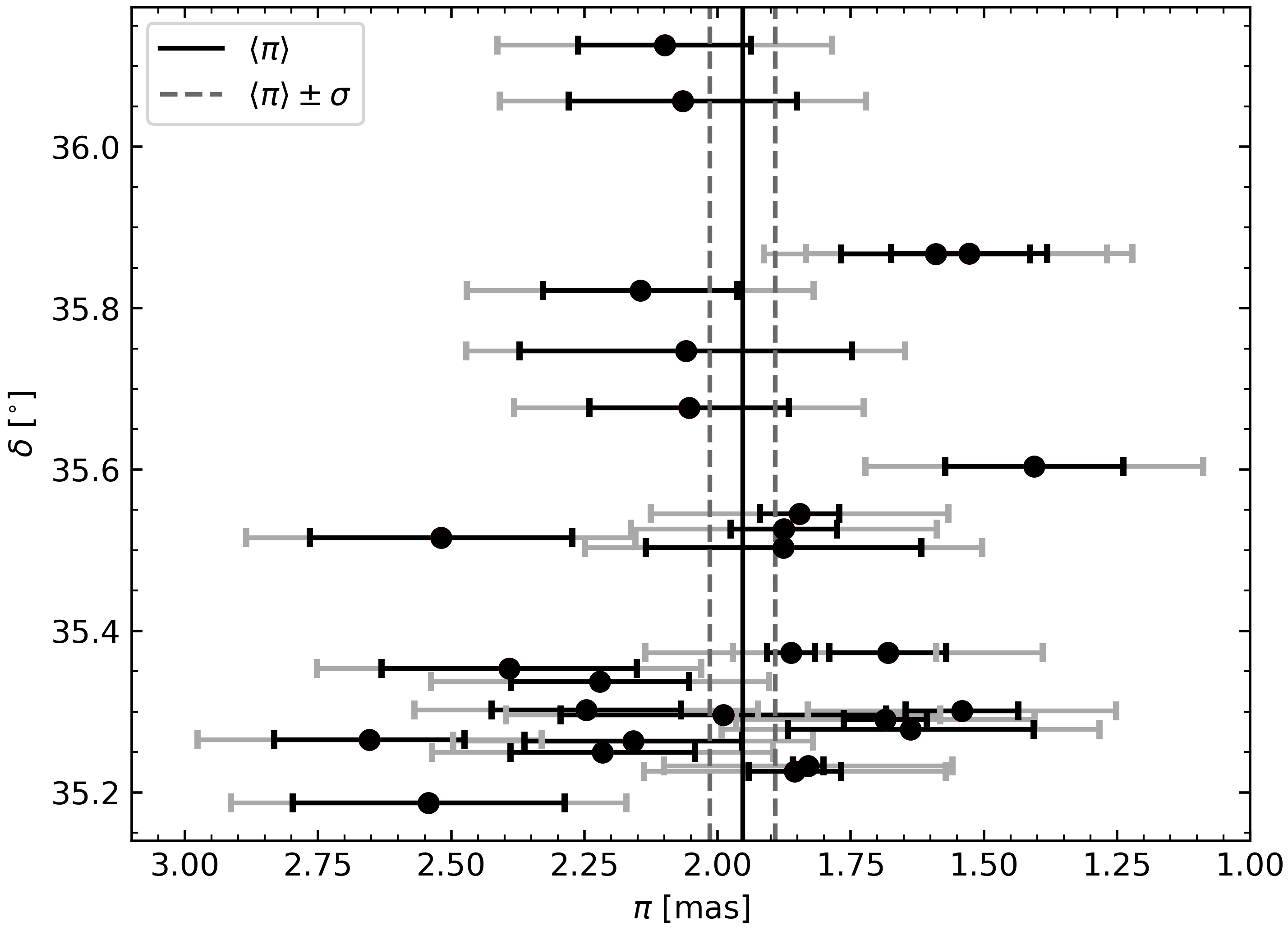
Figure 5: Parallax distribution of the 27 YSOs from Lada et al. (2017) with robust Gaia astrometry (see text). The black points and black error bars show the standard Gaia catalog $\pi$ and $\sigma(\pi)$ values. The grey error bars include the error floor $\epsilon$ calculated to enforce $\chi^{2}=\rm{dof}$, see § 3. Using the grey error bars, the error-weighted mean parallax and the standard error are $\langle\pi\rangle~{}=~{}1.956\,\pm\,0.064$ mas, shown with vertical lines in the plot, which corresponds to $D~{}=~{}511^{+17}_{-16}$ pc. This value is in good agreement with the Zucker et al. (2019) distance.

In Figure 5 we show the parallax distribution of these 27 YSOs. We see that the intrinsic dispersion in the data cannot be fully accounted for by the uncertainties, suggesting that the uncertainties are under-estimates of the true uncertainties. To correct for this we first find the mean value of the parallax, $\mathbf{\langle}\pi\rangle$, the mean error, and resulting $\chi^{2}=\sum_{i=1}^{N}(\pi_{i}-\langle\pi\rangle)^{2}/\sigma_{i}^{2}$, where $\pi_{i}$ and $\sigma_{i}$ are the Gaia-reported values. Using the formal errors, we obtain $\langle\pi\rangle=1.98\pm 0.17\,$mas and a corresponding $\chi^{2}\approx 147$. This value is large compared to the expected range $\chi^{2}=26\pm\sqrt{52}$ for a $\chi^{2}$ distribution with $N-1=26$ degrees of freedom (dof; see Gould, 2003). It is plausible that the true Gaia errors are larger than the reported formal uncertainties in the region of the filament. Measurements can be adversely affected by nebulosity, crowding, binaries, and differential extinction to a substantially greater degree than for field stars (Arenou et al., 2018; Lindegren et al., 2018; Gaia Collaboration et al., 2018a; Zinn et al., 2019; Penoyre et al., 2020; Rao et al., 2020). We therefore define the augmented reported errors as $\sigma_{i}^{\prime}=\sqrt{\sigma_{i}^{2}+\epsilon^{2}}$, where $\epsilon$ is an error floor. We choose $\epsilon$ to enforce $\chi^{2}=26$ using the renormalized errors. We find $\epsilon=0.29$ mas. We measure the error weighted mean parallax and its standard error on the mean of $\langle\pi\rangle=1.956\pm 0.064\,$mas for the parallax, corresponding to $D=511^{+17}_{-16}\,$pc for the distance. The measured distance is consistent with the Zucker et al. (2019) distance of 524${}^{+11}_{-7}$ pc.

To test for a possible signature of inclination in the filament, we fit the $\pi$ values as a function of $\delta$ (Stutz et al., 2018). We find no robust trend, in agreement with the visual impression from Figure 5. Given the small number of data points and their corresponding errors, this is not a strong constraint, and hence the filament could still have significant inclination.

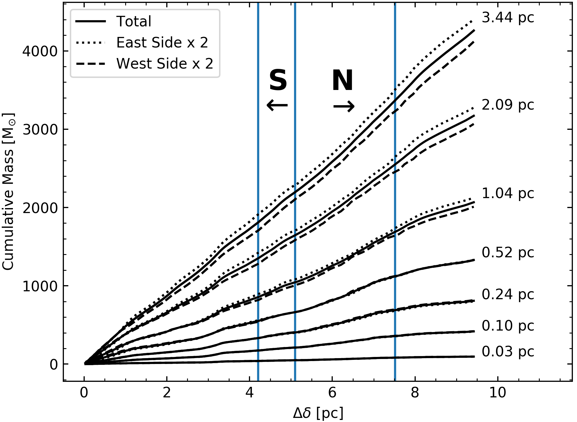
Figure 6: Cumulative mass distribution along the L1482 filament. Different curves indicate different projected radii or impact parameters (see values on the r.h.s.) from the $N_{\rm H}$ ridgeline. Both the east (dotted black lines) and west (dashed black lines) profiles are multiplied by 2 for visual comparison. At all radii the mass as a function of $\delta$ grows approximately linearly. The declination offset, $\Delta\delta$, starts at the bottom of Figure 2 and runs from $\delta\,=\,35.14\mbox{${}^{\circ}$}\rightarrow\delta\,=\,36.18\mbox{${}^{\circ}$}$. The North and South regions (§5.2) are indicated with vertical blue lines.

4 Mass, line-mass, gravitational potential, and acceleration

Here we present the mass distribution analysis based on the Herschel $N_{\rm H}$ map (see § 2.1). In order to carry out this analysis, we start with the identification of the $N_{\rm H}$ ridgeline. We use the $N_{\rm H}$ map (Figure 2) to identify the ridgeline of peak gas surface density as a function of declination $\delta$. Using the $N_{\rm H}$ ridgeline, we separate the map into east and west sides. In Figure 6 we show the cumulative mass along $\delta$ at different projected radii from the $N_{\rm H}$ ridgeline. We show the extents of the North and South regions (see § 5.2).

From this figure we appreciate two important features of the mass distribution. First, at each projected radius, the mass increases almost linearly without jumps along $\delta$. Hence, the cumulative mass distribution is, to first order, only dependent on the projected radius. Second, the distributions are mostly symmetric on each side of the filament, simplifying the geometry of the system. Combined, these features allow us to extract an average cumulative line-mass (M/L) profile for the structures as a whole (Stutz & Gould, 2016).

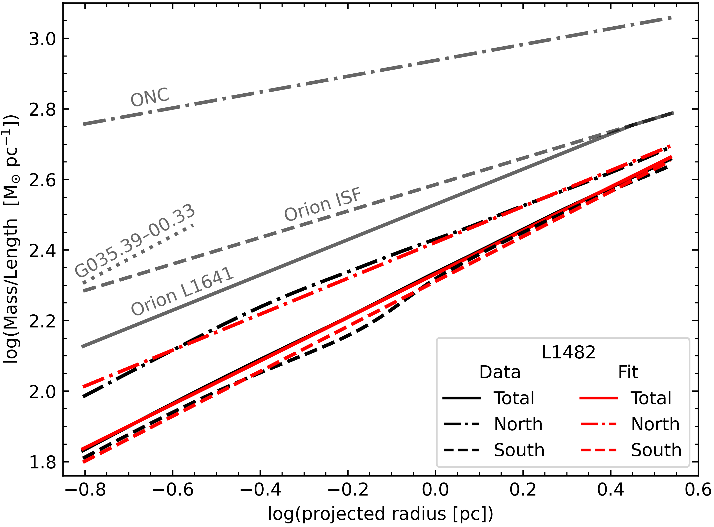
Figure 7: Enclosed line-mass (see Equation 2 and Table 3) versus projected radius from the $N_{\rm H}$ ridgeline for the L1482 filament (black curves) and best-fit power law (red curves). We include the profiles for the North and South regions (see § 5.2 and § 5.3). For comparison, we show $\lambda(\rm{w})$ for Orion ISF (grey dashed curve; Stutz & Gould 2016), Orion L1482 (grey solid curve; Stutz & Gould 2016), the ONC (grey dashed dotted line; Stutz 2018), and G035 (dotted gray line; measured from the Kainulainen & Tan 2013; see § 7 for details of this filament). This figure presents a progression from low to high line-mass regions, where the lowest line-mass region is L1482 South (dashed line) with comparatively few YSOs, and the highest line-mass region is the Orion Nebula Cluster (ONC, Stutz, 2018), with hosting the embedded star cluster by the same name.

We show the enclosed M/L profile of L1482 in Figure 7. We include the profiles for the North and South regions separately. The distributions are well approximated by a power-law down to the resolution limit of the data. We apply a power-law fit (i.e., red-line linear fit to the log-log representation in Figure 7) to the filament profiles, including the North and South regions:

$$\lambda_{app}(w) = \rm{\zeta}\biggl{(}\frac{\textit{w}}{{\rm pc}}\biggr{)}^{\gamma},$$ (2)

where $w$ is the plane-of-the-sky (POS) projected radius; this expression gives the apparent line-mass distribution in the POS (see Table 3 for the values of $\zeta$ and $\gamma$). This demonstrates that the North region has a higher line-mass profile than the South region. Meanwhile, the total line-mass profile of L1482 is lower than those of the Orion L1641, Orion Integral Shaped Filament (ISF), and the Orion Nebula Cluster (ONC, Stutz & Gould, 2016; Stutz, 2018), respectively.

Because of the symmetry and radial dependence of the cumulative mass profiles, and the fact that the line-mass profiles are well-characterized by scale-free power laws down to the resolution limit of the Herschel data (see Figure 6 and 7), we assume a cylindrical morphology for the filament, with axial symmetry around the $N_{\rm H}$ ridgeline. Below we follow the formalism presented in Stutz & Gould (2016) and Stutz (2018) for the calculations of the apparent plane-of-the-sky volume density, gravitational potential, and gravitational acceleration. Table 3 presents the power-law indices and normalizations for the expressions presented below.

Table 3: Line mass, density, gravitational potential, and acceleration profile parameter values.

Region	$\zeta^{g}$	$\beta^{h}$	$\psi^{i}$	$\xi^{j}$	$\gamma^{k}$	Projected length	Total gas mass
	$[\hbox{M${}_{\odot}$}{\rm pc}^{-1}]$	$[\hbox{M${}_{\odot}$}{\rm pc}^{-3}]$	$[(\rm km\,s^{-1})^{2}]$	$[(\rm km\,s^{-1})^{2}{\rm pc}^{-1}]$		[pc]	$[\hbox{M${}_{\odot}$}]$
L1482a	214	10.2	1.45	0.89	0.62	9.4	4260
L1482-Nb	264	12.6	2.63	1.34	0.51	2.3	1090
L1482-Sc	205	9.6	1.27	0.81	0.64	0.9	380
Orion ISFd	385	16.5	6.30	2.40	0.38	7.3	6200
Orion L1641d	338	16.1	3.50	1.80	0.50	23.2	$2\times 10^{4}$
ONCe	866	25.9	27.60	6.40	0.23	0.5	1300
G035f	682	31.5	3.96	2.60	0.66	2.0	822

Note. — Values for the parameters derived in § 4. We include all regions shown in Figure 7.

^a This work, calculated over the range $35.14\mbox{${}^{\circ}$}<\delta<36.19\mbox{${}^{\circ}$}$.

^b This work, calculated over the range $35.71\mbox{${}^{\circ}$}<\delta<35.98\mbox{${}^{\circ}$}$.

^c This work, calculated over the range $35.61\mbox{${}^{\circ}$}<\delta<35.71\mbox{${}^{\circ}$}$.

^d Stutz & Gould (2016).

^e Stutz (2018).

^f Calculated using a $N_{\rm H}$ map derived from Kainulainen & Tan (2013) over the N₂H⁺ region from Henshaw et al. (2014).

Normalization constants:
^g for the M/L profile (Eq. 2).
^h for the volume density (Eq. 4).
ⁱ for the gas gravitational potential (Eq. 5).
^j for the gravitational acceleration (Eq. 6).
^k is the power-law index in the M/L and gas gravitational potential profiles; the power-law index for the volume density is $\gamma-2$ and for the gravitational acceleration is $\gamma-1$.

The apparent volume density is estimated as:

$$\rho_{app}(r) = \frac{\gamma(-\gamma/2)!}{2(-\gamma/2-1/2)!(-1/2)!}\frac{\zeta}{{\rm pc}^{2}}\left(\frac{r}{{\rm pc}}\right)^{\gamma-2}$$ (3)

$$= \beta\left(\frac{r}{{\rm pc}}\right)^{\gamma-2}.$$ (4)

The gas gravitational potential follows as:

$$\Phi_{app}(r)=\psi\bigg{(}\frac{r}{{\rm pc}}\bigg{)}^{\gamma}.$$ (5)

Given that the gravitational acceleration is defined as $g(r)~{}=~{}-\nabla\Phi(r)$, then:

$$g(r)_{app}=-\xi\bigg{(}\frac{\it{r}}{{\rm pc}}\bigg{)}^{\gamma-1}.$$ (6)

The expressions in Equations (2), (4), (5), and (6) represent the plane-of-the-sky inferred quantities. They must be multiplied by the unknown projection factor $\cos(\theta)$, where $\theta$ is the inclination angle of the filament relative to the plane of the sky (see § 3 for inclination discussion). In Table 3 we give $\zeta$, $\beta$, $\psi$, $\xi$, and $\gamma$ values for all regions in Figure 7, under the assumption that $\cos(\theta)=1$.

We also analyze the inner mass distribution of IRDC G035.39-00.33 (henceforth G035), located in the W48 complex at a distance of 2.9 kpc. This cloud has a total mass of $\sim 2\times~{}10^{4}~{}\rm{M}_{\odot}$, presents a filamentary morphology, gas velocity gradients, and low star formation activity in the northern portion (Simon et al., 2006; Kainulainen & Tan, 2013; Nguyen Luong et al., 2011; Henshaw et al., 2014). We start with the 8µm extinction map from Kainulainen & Tan (2013) to derive a $N_{\rm H}$ map of the region. We repeat the mass distribution analysis described above to the subregion analyzed in Henshaw et al. (2014). See Table 3 for the parameters. After the ONC, G035 has the highest line-mass of the regions shown in Figure 7 (see § 7).

5 Filament gas velocities

Gas radial-velocity maps provide velocity gradients, which may be signatures of rotation, outflows, and/or infall in L1482. Measurements of the line widths allow us to scrutinize the non-thermal velocity dispersion. When compared to the gas gravitational potential, we can then evaluate the physical state of the filament (e.g., González Lobos & Stutz, 2019). In our analysis below, we use IRAM 30 m data (§ 2.2) and the Kong et al. (2015) ¹³CO(2-1) data (§ 2.2).

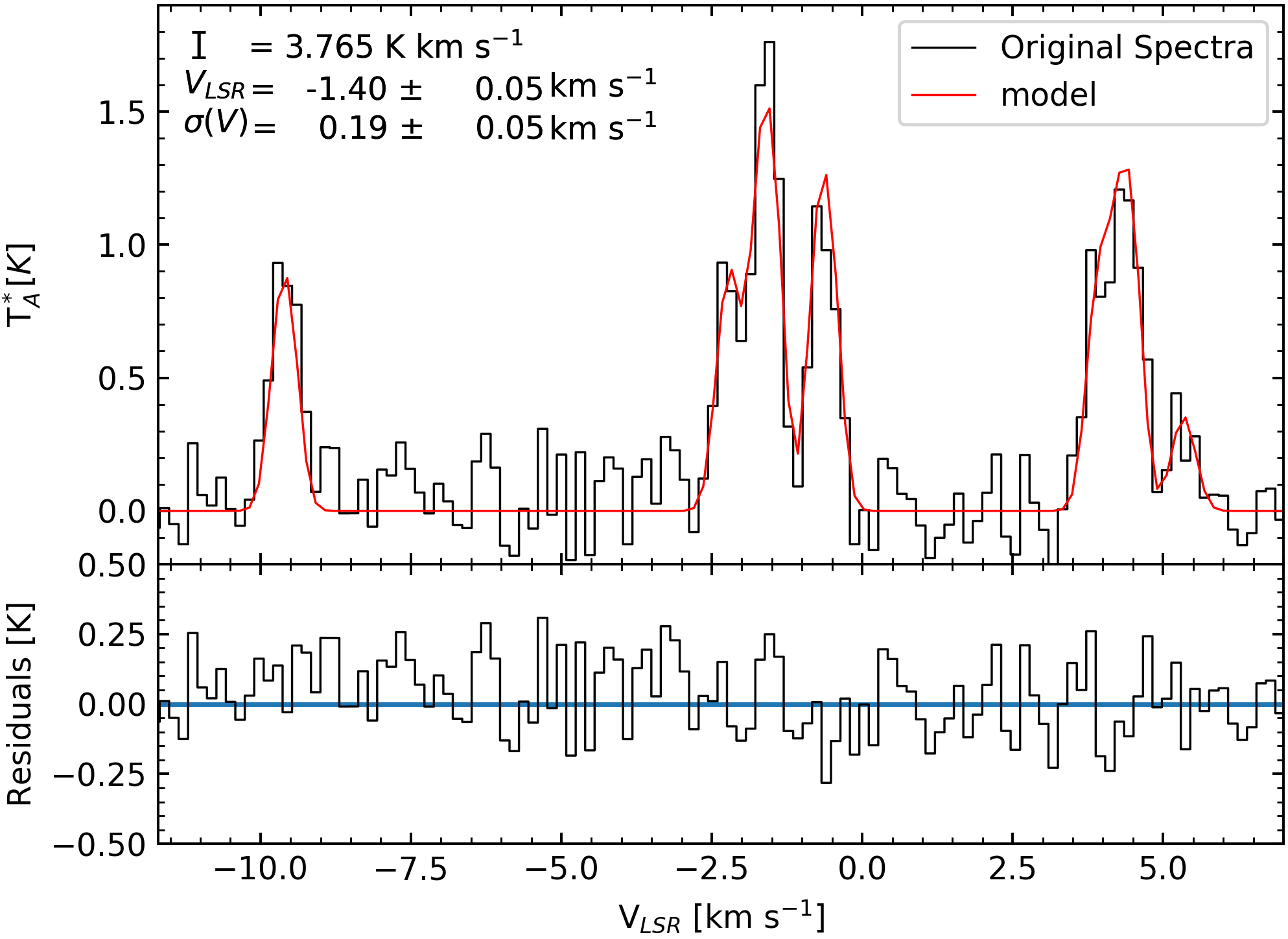
Figure 8: N₂H⁺ line fitting example for a single pixel located at $\alpha$ = 67.6^∘ $\delta$ = 35.97^∘. Top: The original spectrum (black curve) and the fitted model (red curve). In the top left corner we show the integrated intensity, the velocity centroid, and the velocity dispersion. Bottom: The residuals of the fit are shown in black and are centered at y = 0, indicated with a blue line.

5.1 Line fitting

We employ the line-modeling python package PySpecKit (Ginsburg & Mirocha, 2011) to fit line profiles and remove noise from our data. For the line fitting of C¹⁸O, HCO⁺, HNC, and ¹³CO we use a single Gaussian fit, included in PySpecKit. The derived parameters for these tracers are the peak of the spectrum, velocity centroid, and velocity dispersion. To model the hyperfine line structure of N₂H⁺, we use the built-in fitter “n2hp$\_$vtau” (Ginsburg & Mirocha, 2011) that adjusts multiple Gaussians to the raw spectrum. The derived parameters are the excitation temperature, optical depth, integrated intensity, velocity centroid, and velocity dispersion.

To set a signal-to-noise ratio (SNR) threshold for the fitter we need to determine the SNR for each spectrum. We create an error map by taking the RMS ($\sigma_{\rm{rms}}$) values of the spectra in a velocity range without gas emission. We set this velocity range from $-40$ $\rm km\,s^{-1}$ to $-10$ $\rm km\,s^{-1}$ for the IRAM 30 m tracers. The mean $\sigma_{\rm{rms}}$ for each field is shown in Table 2. For ¹³CO we set the velocity range between $-25$ $\rm km\,s^{-1}$ and $-10$ $\rm km\,s^{-1}$. For C¹⁸O, HCO⁺, and HNC we find a SNR threshold of 3.5. For both ¹³CO and N₂H⁺, SNR = 3 produces good fitted models. These values remove most of the noise without affecting the emission from the filament.

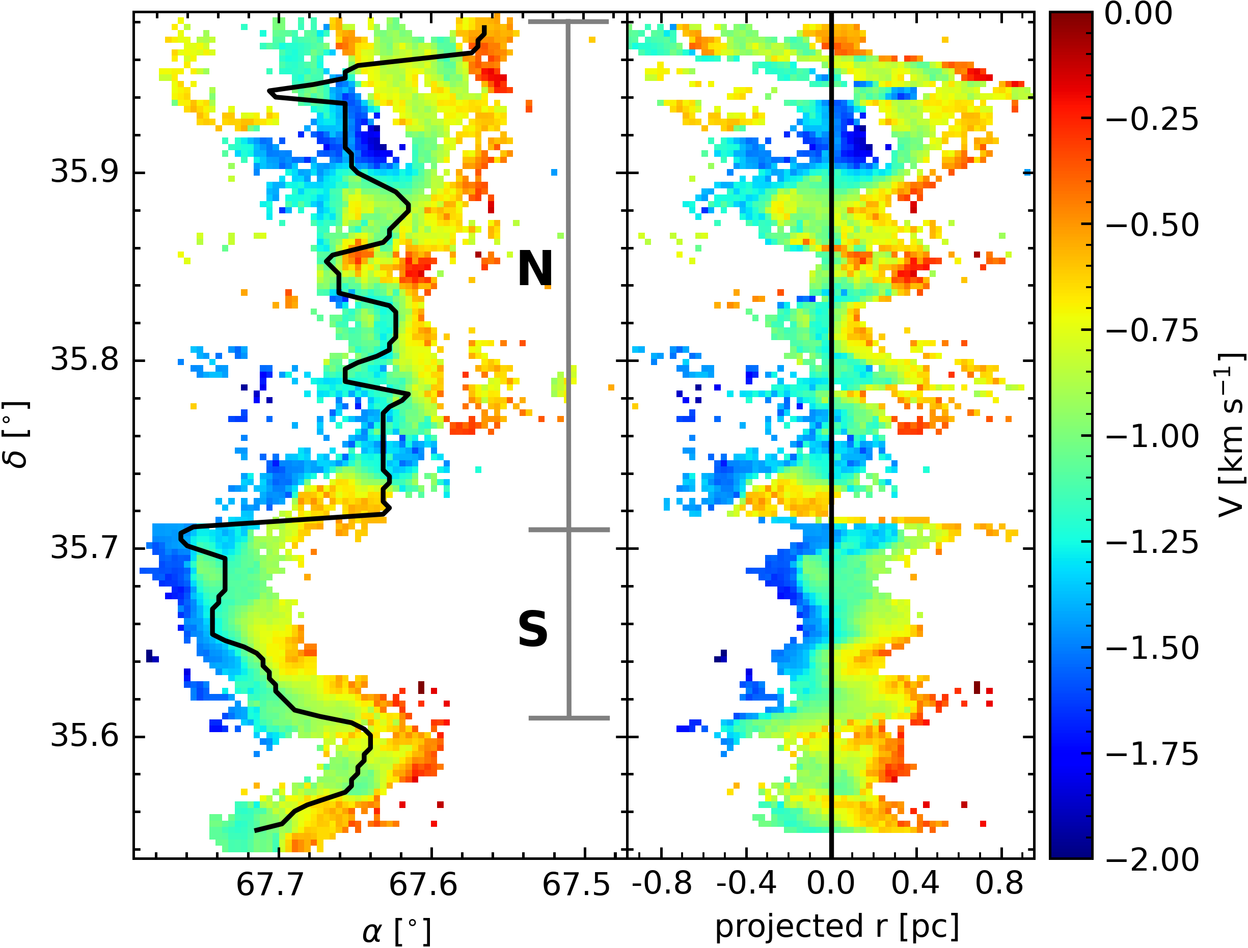
Figure 9: Left: C¹⁸O first-moment (mean velocity) map. The black curve shows the $N_{\rm H}$ ridgeline. Right: C¹⁸O first-moment map aligned to the $N_{\rm H}$ ridgeline (straight black line). Negative r values indicate the east side of the filament. We observe a velocity gradient (VG) perpendicular to the long axis of the filament, going from blue- to red-shifted velocities from east to west. This rotation signature is particularly evident in the southern portion of the filament (extent indicated with the vertical grey bar in the left panel), see text.

The fitting process requires a user-defined starting point inside the cube and initial guesses to fit the spectrum in this pixel. For all tracers we use starting values based on the peak of the spectra, first-moment map, and second-moment map values. For N₂H⁺ we also adopt an excitation temperature and optical depth of 6 K and 0.5 respectively. These last two parameters were selected by testing different values until obtaining fitter result convergence. In Figure 8 we show one pixel example of the N₂H⁺ modeled cube. In the top panel we show the original spectrum (black line) and the fit (red line). In the lower panel we show the residuals.

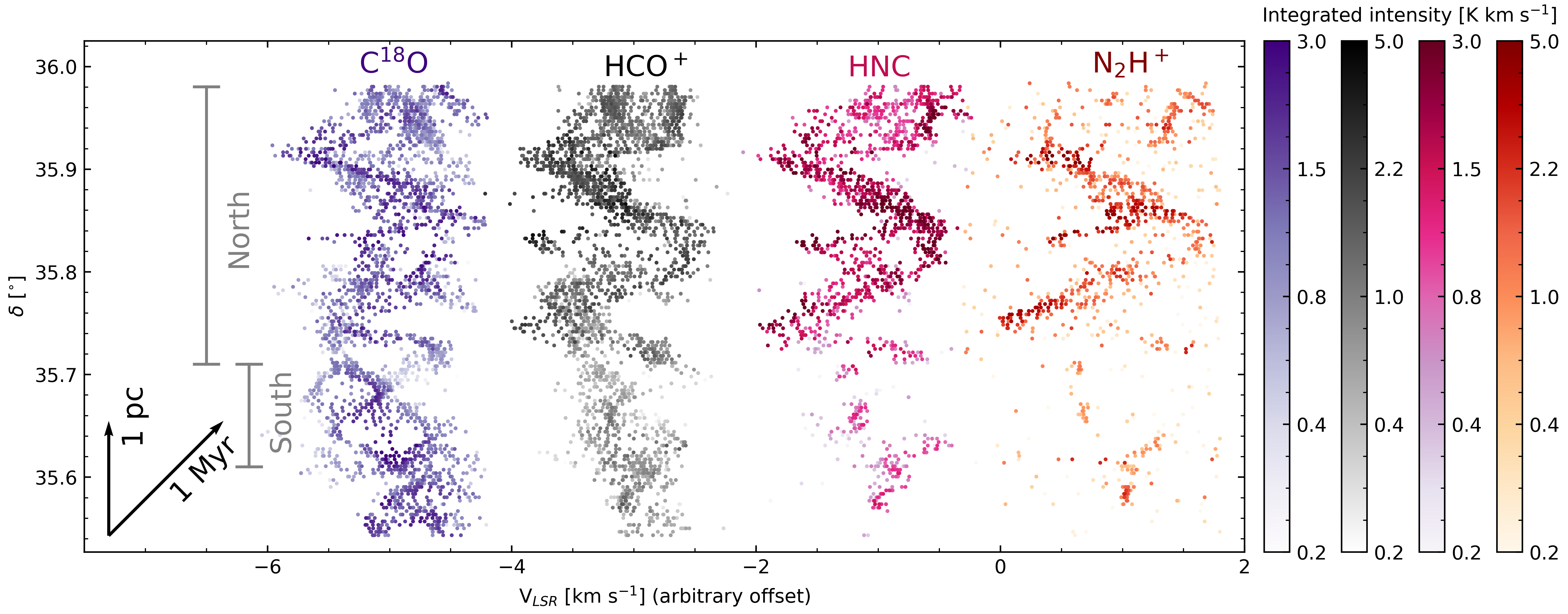
Figure 10: Intensity-weighted position-velocity (PV) diagram: C¹⁸O, HCO⁺ and N₂H⁺ are shown with arbitrary velocity offsets of $-4~{}\rm km\,s^{-1}$, $-2~{}\rm km\,s^{-1}$, and $+2~{}\rm km\,s^{-1}$, respectively, from HNC. The color bars are logarithmic in scale to enhance the visibility of structures with lower intensities. The gray vertical lines indicate the extent in $\delta$ of the North and South regions defined in § 5.2. The black vertical arrow shows the spatial scale of 1 pc, and the diagonal arrow indicates a timescale of 1 pc/$\rm km\,s^{-1}$ $\approx$ 1 Myr.

For the single-component IRAM 30 m models we remove artifacts produced by bad fits, located in the outer parts of the filament at low SNR. We define SNR = I_peak/$\sigma_{\rm{rms}}$, where I_peak is the peak intensity of the modeled spectra and $\sigma_{\rm{rms}}$ is derived from the original data in the same velocity range as in the fitter. We measure the SNR in all cubes. For consistency with the fitter procedure we remove spectra with SNR $<$ 3.5. We obtain good results with this approach, giving us clean models to work with.

In Figure 9 we present the cleaned version of the modeled C¹⁸O mean line velocity (moment 1) map. In the left panel we show the standard moment 1 map, while in the right panel we align the map at each $\delta$ to the $N_{\rm H}$ ridgeline. From this figure it is immediately obvious, especially in the South region, that we detect a clear and confined velocity gradient (VG) going from negative $\rightarrow$ positive velocities from east $\rightarrow$ west, “hugging” the $N_{\rm H}$ ridgeline. Gas velocity gradients have been detected in different filamentary systems with different proposed origins such as filamentary rotation, shear, gas inflow, and cloud-cloud collisions (e.g., Uchida et al., 1991; Jiménez-Serra et al., 2014; Lee et al., 2014; Fernández-López et al., 2014; Henshaw et al., 2014). We study this velocity gradient in detail in § 6.

For ¹³CO, C¹⁸O, HCO⁺, and HNC the line widths present large variations along $\delta$. Here we test whether the large velocity dispersions are the result of fitting a double-component or more complex line profile with a single Gaussian by using a double-component model. From the double velocity-component fitting results, we find that most spectra can be fitted with only one Gaussian, while the secondary component generally has low SNR compared to the defined threshold. In order to identify spectra with reliable double components we define a temperature threshold. If the peaks of both components are above the threshold we consider them as well-detected. For C¹⁸O, we identify two well fitted velocity components when we set this threshold to 0.8 K, almost three times the noise value of Field 1 (see Table 2). From the above procedure, we conclude that $\sim$13% of the C¹⁸O data contains double-components. These are mainly located at or near the $N_{\rm H}$ ridgeline. When fit individually, the components of these spectra have slightly lower line widths compared to the single components. The North region presents more double-component spectra compared to the South, as we expect (see discussion below). In order to avoid line-width and velocity contamination or confusion in the subsequent analysis, we remove the pixels in which double-component spectra are detected (see Figure 11).

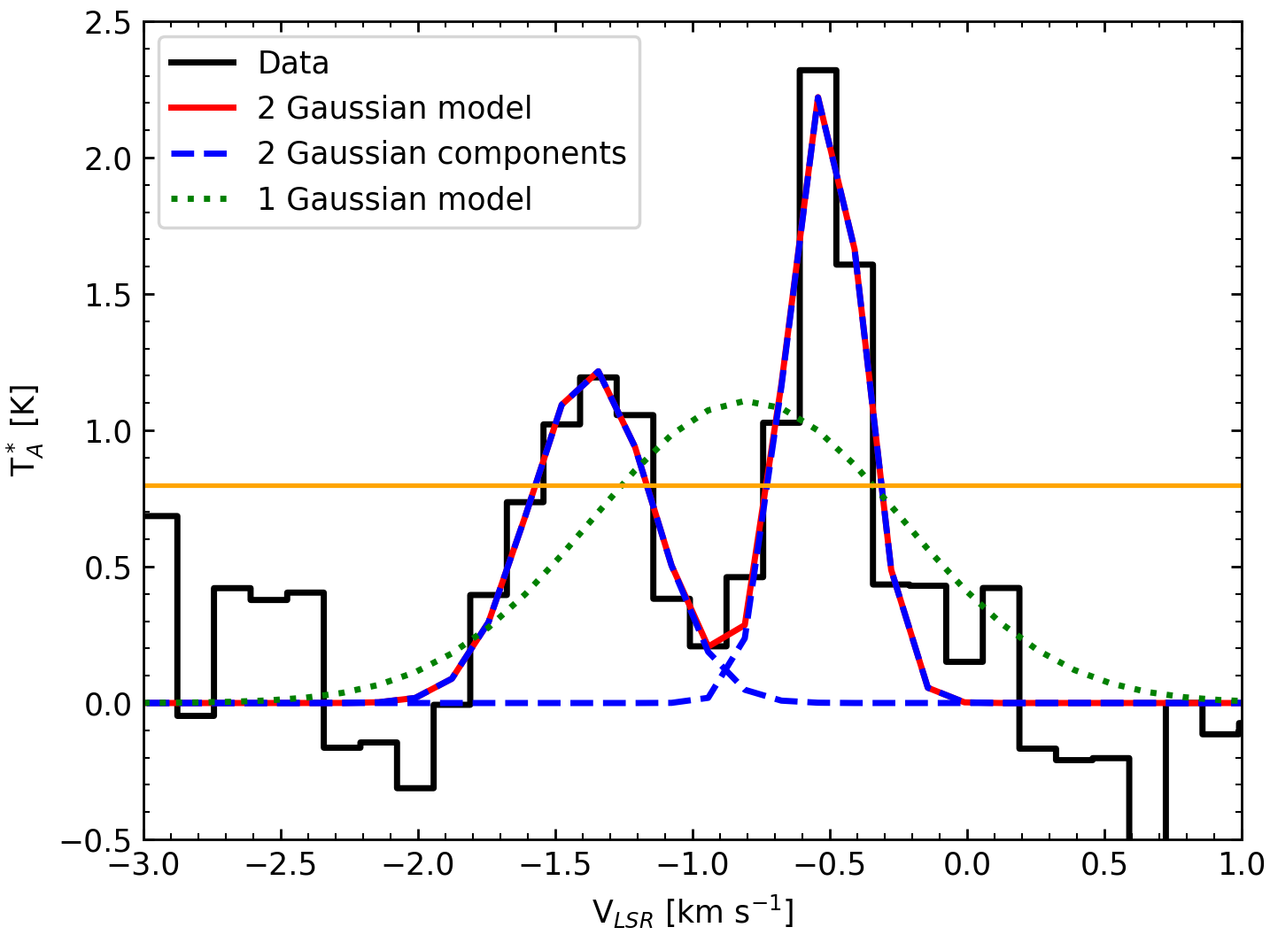
Figure 11: Double Gaussian spectrum example. The raw data is shown in black. The double Gaussian fit is shown in red and its components with dash blue lines. The single Gaussian fit is presented with a green dotted line. We indicate the intensity threshold with a solid orange line.

In short, the single component spectra dominate the spectral cubes, and the measured velocities and the line widths of the fitting procedure agree well with previous observations of L1482 (e.g., Li et al., 2014; Kong et al., 2015). The removal of the double component spectra does not affect the results of our analysis below. Moreover, we find no C¹⁸O or HCO⁺ spectra exhibiting a clear blue asymmetry or an inverse P-Cygni like profile. Such profiles would indicate infall along the line of sight (e.g., Myers et al., 2000; Evans et al., 2015; Smith et al., 2012). The absence of an infall signature may be caused by the resolution of our data. We conclude that our procedure adopting single-component fits is robust. In the sections that follow we use these to analyze the velocity structure of L1482.

5.2 Intensity-weighted position-velocity diagrams

Using the fitter results described above, we generate intensity-weighted position-velocity (PV) diagrams for the IRAM 30 m data, presented at different velocity offsets in Figure 10. Here we show the best-fit gas velocities as a function of $\delta$ along the filament, weighing by the integrated line intensity. This technique is described in detail in González Lobos & Stutz (2019); it removes noise present in the traditional PV diagram method while highlighting structure that would otherwise be muddled or invisible (see their Figure 3 and 4).

In Figure 10, we see similar structures in C¹⁸O and HCO⁺ across most of the extent of the filament. High density gas, as traced by N₂H⁺, is mostly not detected at $\delta\lesssim 35.71\mbox{${}^{\circ}$}$. Moreover, at $\delta\sim 35.71\mbox{${}^{\circ}$}$ there is a discontinuity in the filament that is coincident with a jump in the $N_{\rm H}$ map (see Figure 2 and 9). This jump marks the transition between two physically distinct filament environments. Above this location we have a higher M/L region, which contains more YSOs (see Figure 3), while below the jump we find a more confined filament with lower M/L values (see Figure 7 and Table 3). We therefore divide the filament into two subregions. The northern region encompasses $\delta=35.71\mbox{${}^{\circ}$}\rightarrow 35.98\mbox{${}^{\circ}$}$. The southern region encompasses $\delta=35.71\mbox{${}^{\circ}$}\rightarrow 35.54\mbox{${}^{\circ}$}$.

In Figure 10 we observe in all tracers the presence of elongated structures with gradients. These have slopes, given the axis ratio of the plot, approximately consistent with $1$ Myr timescales (but see discussion below). Along the filament we also identify structures that have an appearance consistent with wrapping or winding, perhaps most obvious in C¹⁸O in the southern portion of the filament. In this region the filament has a clear “zig-zag” morphology in $N_{\rm H}$ (see Figure 2), potentially indicating a cork-screw or helical-like morphology in 3D. Overall, the velocity wiggles are reminiscent of the structures in the Integral Shaped Filament (ISF) in Orion A (see Figure 4 of González Lobos & Stutz, 2019).

At $\delta\sim 35.83$^∘ we observe a large spike in velocity where the filament appears to have two well-separated velocity components, most obvious in HCO⁺, HNC, and to a lesser extent in N₂H⁺. The region at the east of the ridgeline in the C¹⁸O first moment map (see Figure 9) exhibits compact blue- and red-shifted velocities near this location. These alone might plausibly indicate some YSO-associated outflow activity. However, the appearance of this feature, albeit at fainter levels, in N₂H⁺ indicates that this velocity pattern persists in the denser gas, where outflow signatures may be less likely to arise.

The feature bears some resemblance to the N₂H⁺ velocity spike observed by González Lobos & Stutz (2019) in Orion A at $\delta\sim 5.4$^∘, that is, in the center of the ONC gas filament. In the present case, the maximum velocity shift between the two N₂H⁺ loci is $\sim 1.5$ $\rm km\,s^{-1}$, while in the ONC it is $\sim 4$ $\rm km\,s^{-1}$. The C¹⁸O velocity pattern continues to the South to $\delta\sim 35.74\mbox{${}^{\circ}$}$, progressing through a series of back-and-forth wiggles until $\delta=35.71\mbox{${}^{\circ}$}$, where the filament breaks and jumps over both in projected position (in the $N_{\rm H}$ map, and see above) and in velocity, which may bear some relation to the drastic break in the ISF near $\delta\sim-5.5\mbox{${}^{\circ}$}$. The general appearance of the velocity patterns in L1482 is somewhat similar to the ISF González Lobos & Stutz (2019), but with smaller amplitudes.

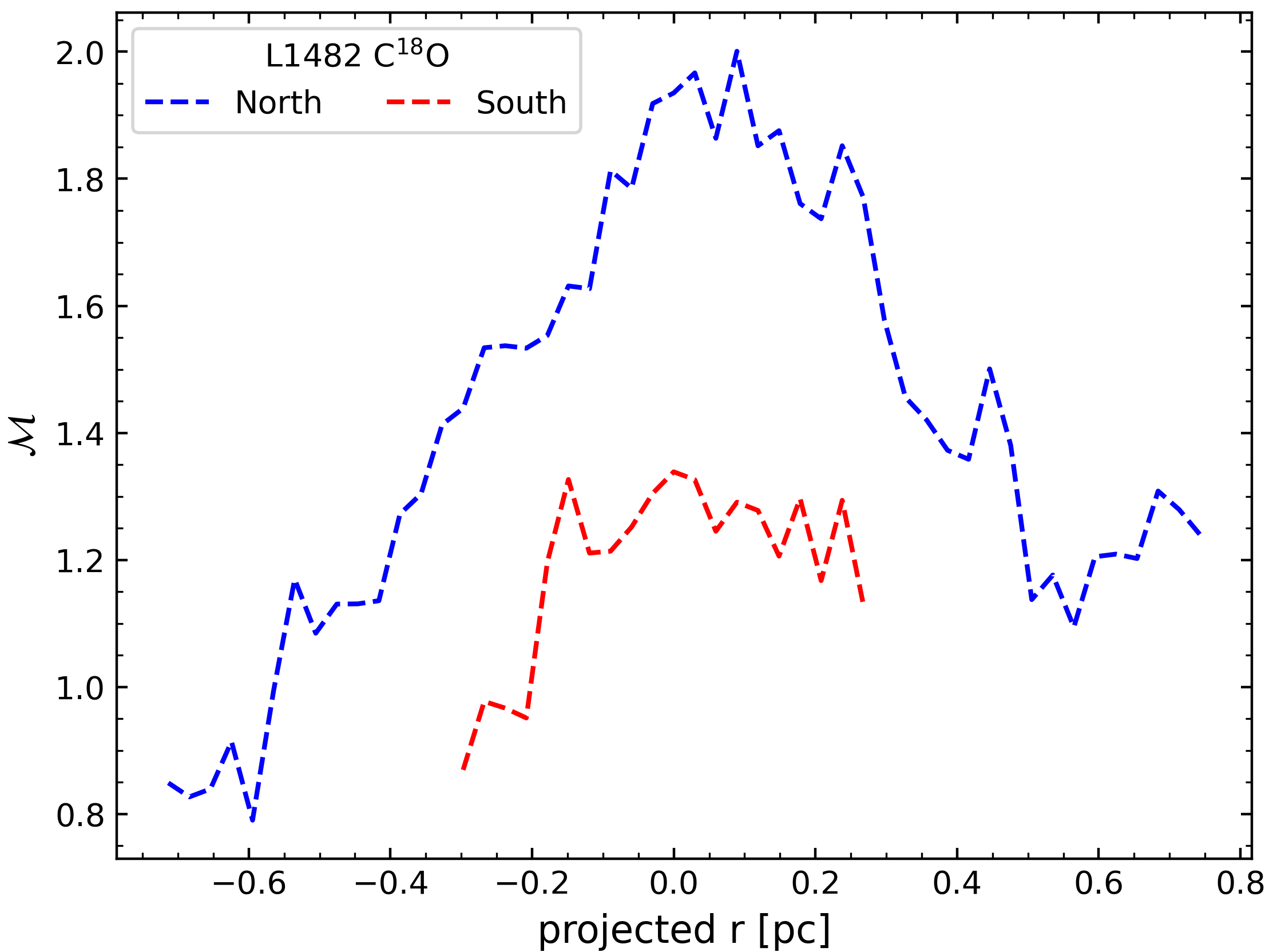
Figure 12: C¹⁸O North (blue) and South (red) Mach number ($\cal M$) profiles. The tracers present supersonic line-width profiles, and large differences between the two regions.

5.3 Mach number profiles across the filament

Here we analyze the gas line-widths. Variations in the velocity dispersion across the filament are useful for identifying variations in the gas kinematics within the filament (see, e.g., Federrath, 2016). In the top right panel of Figure A.1 we show the C¹⁸O second-moment map. In what follows, we compare the line-width profiles in the North and South regions of L1482.

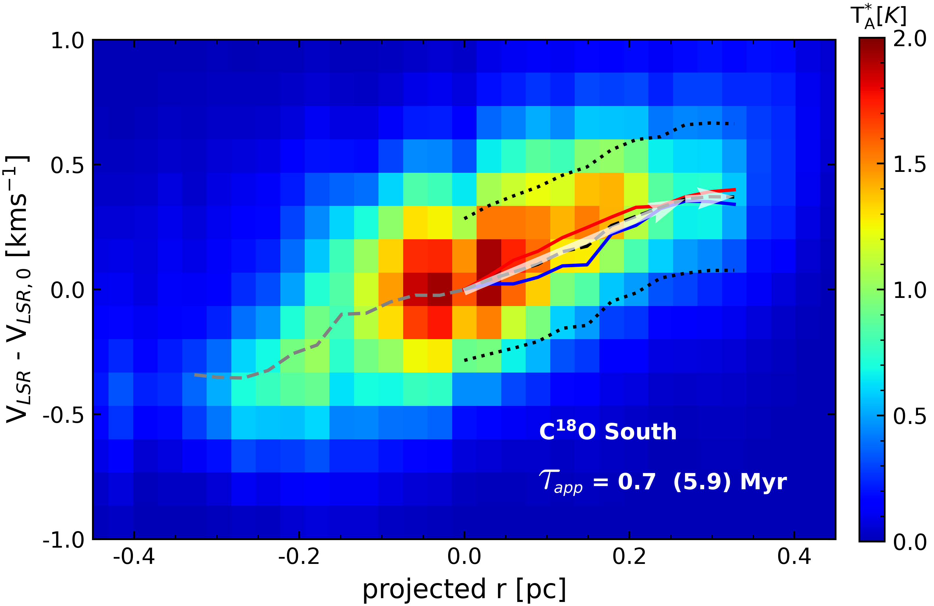
Figure 13: Velocity vs. projected radius map for C¹⁸O L1482 South. Negative r values indicate the east side of the filament while positive r values indicate the west side, relative to the dust ridgeline. The dashed grey curve shows the velocity gradient at r $\leq$ 0 pc, while the blue curve shows the same r $\leq$ 0 pc flipped to the r $\geq$ 0 pc side for comparison with the r $\geq$ 0 pc red-shifted velocity gradient (red curve) of the filament. The dashed black curve shows the mean of the blue and red velocity gradients. The dotted black curves show the mean upper and lower bounds on the radial velocity between the each side of the filament, as measured by the intensity-weighted standard deviation of the velocity. The translucent white arrows represent the velocity profile derived from the best-fit line to the black dashed curve (the mean observed velocity profiles). The velocity profile flattens at $r\,\sim\,0.25$ pc, as captured by the slopes of the inner and outer arrows. The associated timescales ($\tau_{app}$ = 1/VG_app, where VG_app is the velocity gradient) are shown in the bottom right corner.

We measure non-thermal motions in the gas through the non-thermal line width ($\sigma_{\rm{NT}}$) and Mach number ($\cal M$). We derive the non-thermal line width as $\sigma_{\rm{NT}}\,=\,\sqrt{\sigma_{obs}^{2}-kT_{k}/m}$ (Liu et al., 2019; González Lobos & Stutz, 2019), where $\sigma_{obs}$ is obtained from the moment 2 velocity dispersion data, $m$ is the mass of the molecule, $k$ is Boltzmann constant, and $T_{k}$ is the gas kinetic temperature. We assume that T_k is equal to the dust temperature T_d in the filament, where the hydrogen densities are higher than 10⁴ cm^-3 and the gas and dust are coupled (e.g., Lippok et al., 2013). In appendix B we fit a softened power-law profile to the Herschel $T_{\rm d}$ map (see § 4). We derive the Mach number profile $\cal M$ = $\sigma_{\rm{NT}}/\rm{c}_{s}$, where c${}_{s}\,=\,\sqrt{kT_{k}/\mu m_{\rm H}}$ is the sound speed, $\mu$ = 2.33 is the mean molecular weight, and $m_{\rm{H}}$ is the hydrogen atomic mass (Liu et al., 2019; González Lobos & Stutz, 2019).

In Figure 12 we present the mean C¹⁸O Mach number profiles as a function of distance from the $N_{\rm H}$ ridgeline in the North and South regions separately (see above and González Lobos & Stutz, 2019, for a similar analysis in the ISF). C¹⁸O has a mildly supersonic profile (${\cal M}\sim 1.2$) in the South but more elevated supersonic profile in the North. For C¹⁸O North, the portion of the filament with actual star formation, the profile peaks toward the filament ridgeline, as opposed to decreasing with density toward the center. This centrally increasing trend is the opposite of that found in the simulations of Federrath (2016). They measure the Mach number profiles in simulations that aim to capture the primary agents that will affect the velocities, such as gravity, turbulence, magnetic fields, and jet and outflow feedback, all of which should be in operation in the CMC/L1482 North filament. In contrast, when we look in the South, the Mach number profile is almost flat over the extent that we are able to probe. In either the North or the South, over the spatial scales that we probe, we observe no transition to a subsonic regime as reported in Federrath (2016). The elevated values of $\cal{M}$ that we observe could be caused by various observational effects, of which line-of-sight averaging and spatial resolution may be the first-order culprits. Both these effects may broaden the measured line-widths to some extent. However, with a higher density tracer such as C¹⁸O, we do not expect these effects to be dominant.

As already noted above and by González Lobos & Stutz (2019), our measured Mach number profiles can be compared to simulated profiles, similar to those presented in Federrath (2016) and in particular their Figure 5, so long as the simulations capture the high mass regime (which the Federrath 2016 simulations do not). Moreover, these should be compared to observations in other filaments at the same mass regime, such as those presented in González Lobos & Stutz (2019). See discussion below.

6 C¹⁸O Velocity gradient across the filament

Here we characterize the velocity gradient of C¹⁸O across the filament in the South region, observed as a prominent feature in Figure 9. Given the confined symmetry of the gradient on either side of the ridgeline (see also A.1), the fact that it is detected along the entire $\delta$ range that we probe, and the lack of clear infall detections on these scales (see above), this signature is consistent with a rotational origin as opposed to arising from, for example, cloud-cloud collisions (e.g., Olmi & Testi, 2002; Fukui et al., 2018).

We characterize the magnitude and spatial extent of this gradient as follows. In Figure 13 we show the C¹⁸O velocity vs. radius map and corresponding gradients. In order to measure the gradients we must first construct mean aligned velocity vs. radius maps. We accomplish this by:

1. Aligning the data cube w.r.t. the $N_{\rm H}$ ridgeline in $\delta$ (see Figure 9).

2. Marginalizing over the aligned $\delta$ coordinates in the South region.

3. Fitting the gradient in projected radius vs. velocity.

We obtain the intensity-weighted mean velocity as a function of radius, shown in Figure 13 as the blue and red curves, and the intensity-weighted standard deviation of the velocity distribution at each radii, represented with dotted black curves in the figure. Since we wish to compare a single velocity gradient, we average the blue-shifted (east side) and red-shifted (west side) velocity profiles (mean profiles are shown as the dashed black curve in Figure 13). We then fit a line to these mean V(r) curves (shown as white arrows) to obtain the velocity gradients (VG_app), or equivalently timescales $\tau_{app}=1/\rm{VG}_{app}$, presented as translucent white arrows in the figure with corresponding inner (outer) timescales of 0.7 (5.9) Myr. As above, we must correct for the (unknown) inclination of the filament by dividing VG_app by the factor $\cos(\theta)$, where $\theta$ is (as defined above) the inclination of the filament relative to the plane of the sky.

Figure 13 reveals that the C¹⁸O South velocity profile (and therefore associated gradients) is approximately anti-symmetric about the $N_{\rm H}$ ridgeline (which defines $r=0$), as illustrated by the similarity between the red- and flipped blue-shifted curves in the diagram. Moreover, the transition to the shallower gradient on at $r\sim\,0.25~{}{\rm pc}$ is also anti-symmetric. This high degree of anti-symmetry lends very strong support to the rotational interpretation of the velocity profile. Moreover, the inner gradient is approximately constant with radius. This may imply, to first order, solid-body rotation of the filament about the long axis. We return to this in § 7 below. To second order, the diagram exhibits departures from this simple model, which we discuss below. In the North region, the C¹⁸O velocity field has a more complex structure (see Figure A.1). Given that the North region has more fragmentation and correspondingly a larger number of protostars, and its M/L profile as a function of radius is both larger in amplitude and shallower in slope, we interpret these differences as due to the combined action of gravity and rotation, as opposed to the South wherein rotation appears primary in setting the transverse filament radial velocity field. We also note that some of the variations between the North and South may arise from differing but unknown average inclinations between the two regions.

In addition to the differences between the North and South, we find that in particular, in the C¹⁸O South diagram (Figure 13) the gradient exhibits a clear and regular radial dependence, mentioned above. In the inner portion of the filament the gradient appears somewhat steeper, indicating a shorter timescale ($\tau_{app}~{}=~{}0.7$ Myr), while the outer portion transitions to a shallower gradient and correspondingly longer timescales. At a radius of $r\,\sim\,0.25$ pc, the velocity profile flattens significantly, departing from the regular velocity pattern that we observe at smaller $r$. This outer flatted region has a gradient consistent with timescales of $\tau_{app}\,\sim 5.9$ Myr (see discussion below).

Moreover, such structures will benefit from detailed modeling of the velocity field. We defer this investigation to future work using, e.g., the POLARIS line radiative transport modeling capabilities (see e.g., Reissl et al., 2018a, b).

7 Discussion

In Figure 13 we have show that the filament exhibits a clear, regular, and linear velocity profile pattern consistent with rotation. To first order, the inner portion of the velocity profile is consistent with solid body rotation. However, clear departures from this simple model are obvious: the velocity profile has a clear break at $r\,\sim\,0.25$ pc, where the velocity profile transitions to a shallower gradient. Moreover, in Figure 12 we show that the gas line-widths and thus non-thermal motions are only moderately supersonic (with Mach numbers $\sim$ 1.2).

The question that we must address now is how the gas motions, inferred from the rotation signature (§ 6), compare to gravity (§ 4). We do this by comparing the gravitational force to the centripetal force taking advantage of the simplicity of solid-body rotation implied by the linear appearance (to first order) of the gradients presented in Figure 13 (also see § 6). We estimate the centripetal force as:

$$\textrm{F}_{c}(r)=ma_{c};\qquad a_{c}=\frac{v^{2}}{r\cos^{2}(\theta)};$$ (7)

where $m$ is the gas mass, $\theta$ is the inclination of the filament relative to the plane-of-the-sky, and $v$ is the velocity profile at each radii (see Figure 13). The force of gravity is given by:

$$\textrm{F}_{g}(r)=mg(r)=mg_{app}(r)\cos(\theta),$$ (8)

where $g_{app}(r)=\xi\left(\frac{r}{{\rm pc}}\right)^{\gamma-1}$ is the gravitational acceleration from Equation (6) and Table 3. From Equations (7) and (8), we obtain the ratio

$$\frac{{\rm F}_{c}}{{\rm F}_{g}}=\frac{v^{2}}{rg_{app}(r)\cos^{3}(\theta)}=\frac{v^{2}{\rm pc}^{-1}}{\xi\cos^{3}(\theta)}\left(\frac{r}{{\rm pc}}\right)^{-\gamma},$$ (9)

or

$$\frac{{\rm F}_{c}}{{\rm F}_{g}}=\frac{{\rm pc}}{\tau_{app}^{2}\xi\cos^{3}(\theta)}\left(\frac{r}{{\rm pc}}\right)^{2-\gamma},$$ (10)

where $\xi$ and $\gamma$ are listed in Table 3.

In Figure 14 we present the apparent (plane of the sky) $\rm{F}_{c}/\rm{F}_{g}$ profile for the South portion of the filament as traced by C¹⁸O. The basic features of this diagram show that the role of rotation relative to gravity increases with radius until $r\,\sim\,0.25$ pc, inside of which the timescales are $\sim\,0.7$ Myr. At $r\,\sim\,0.25$ pc gravity takes over, regulating the filament structure just when the rotational profile would imply break-up or near break-up of the filament.

Moreover, the velocity gradient (on both sides of the filament) is very smooth and regular (see Figure 13), which can be interpreted as the filament being in a dynamically relaxed state. To arrive at such a state, the filament must have undergone a $\sim$ couple of orbits. This then raises the question of timescales. The outer timescale ($\sim\,6$ Myr) is long compared to the inner one, implying that this structure is stable and long-lived, with a lifetime of $\sim$ a few times $6$ Myr. Gómez & Vázquez-Semadeni (2014) and Gómez et al. (2018), based on simulations with and without magnetic fields, find stable and long-lived filamentary structures with approximately similar lifetimes. They attribute these longer timescales to the stability imparted by mass accretion from the immediate environment. This agreement between the timescales we measure here and the previously simulated ones is encouraging. However, the comparison may be limited as the simulated filaments in Gómez & Vázquez-Semadeni (2014) and Gómez et al. (2018) have lower line masses ($\sim\,40\,$M_⊙pc^-1), are embedded in lower mass clouds, and do not show obvious rotation signatures.

If the inclination is non-zero, the role of rotation will be larger compared to gravity, driving the outer force ratio profile closer to unity, and thus closer to break-up. The basic appearance of this diagram therefore implies outside-in evolution of this filamentary structure as the action of gravity and the removal of angular momentum progressively remove support, allowing for progressive mass concentration (see Figure 7) and eventual star formation to take place.

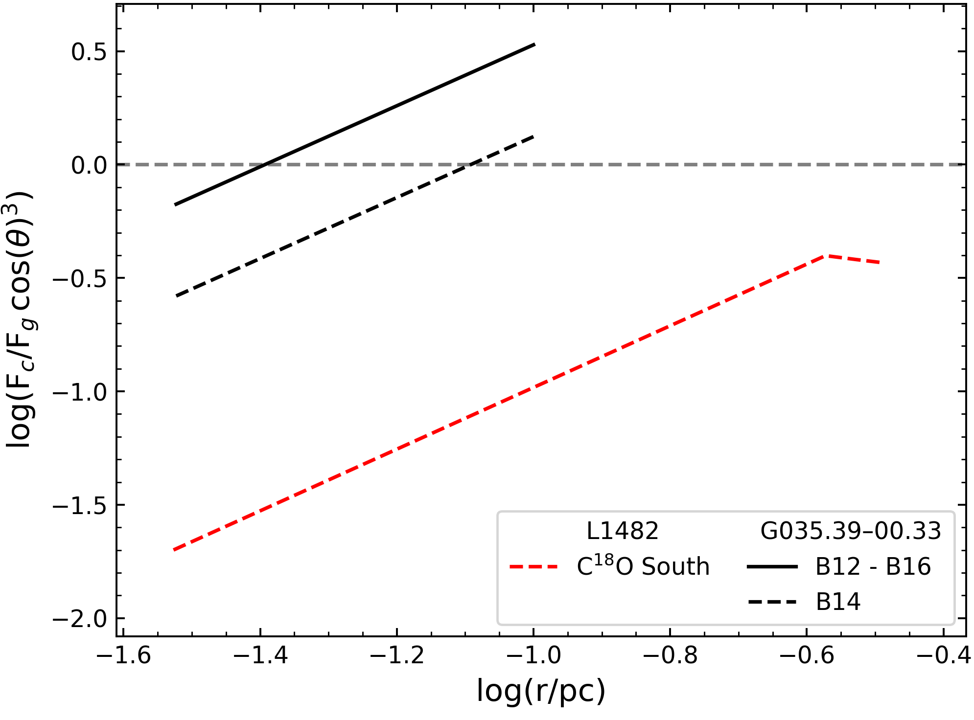
Figure 14: Ratio between the centripetal (F_c) and gravitational (F_g) forces (see Eq. 9). We represent the C¹⁸O South profile with a dashed red line. We include the profiles of slices B12-B16 (black solid line) and B14 (black dashed line) from the IRDC G035 (Henshaw et al., 2014). We show F_c/F_g = 1 with a dashed gray line. These curves, taken at face value, assume $\cos(\theta)=1$, that is, that the filament is not inclined relative to the plane-of-the-sky (see text). For C¹⁸O South we see that gravity dominates over rotation, presenting a turning point at r $\sim$ 0.25 pc. If the inclination of the filament is significant, then rotation will be more dominant.

In Figure 14 we also include the $\rm{F}_{c}/\rm{F}_{g}$ profile for the G035 (e.g., Henshaw et al., 2013; Jiménez-Serra et al., 2014) N₂H⁺ data presented in Henshaw et al. (2014), which has been previously proposed to be in an early evolutionary state. The gas kinematics in this filament exhibit a velocity gradient, with an east to west orientation, similar to L1482. These authors measure a gradient of $-$13.9 $\rm km\,s^{-1}$ pc^-1, for which $\rm{F}_{c}/\rm{F}_{g}$ profile is presented as the solid black line in Figure 14, labeled as “B12 - B16” (see appendix of Henshaw et al., 2014). However, we note that their figures are consistent with a somewhat shallower average gradient of $-$8.7 $\rm km\,s^{-1}$ pc^-1, which $\rm{F}_{c}/\rm{F}_{g}$ profile, which we present as a dashed black line in the same figure. Whatever measure of rotation, G035 appears much more rotationally dominated compared to the L1482 filament. This may partially be caused by the higher density tracer used by Henshaw et al. (2014), or the proposed early evolutionary state of the G035 filament (Henshaw et al., 2013). If the latter, the G035 filament may not have had time to dissipate its angular momentum to collapse toward cluster formation. Another possibility is that the inclinations of L1482 versus G035 are different, which may account for some of the observed differences. At present we have no strong constraints on the inclination for either system.

If the L1482 filament inclination is significant, then rotation will play a larger role. In § 3 we find no significant correlation between $\delta$ and $\pi$ over the filament as a whole. As discussed, this represents a weak constraint on the system inclination due in part to the small number of Gaia-detected YSOs and their corresponding $\pi$ errors. Meanwhile, the clear “zig-zag” plane-of-the-sky morphology of the South region as a whole may indicate a corkscrew or “pig tail”-like morphology (and see below). Such undulations would cause us to again underestimate the role of rotation relative to that of gravity. Hence the basic appearance of Figure 14 is consistent with rotation playing a significant role in the South while being comparatively less dominant in the North, which is clearly gravitationally dominated since it is presently forming stars, and has a larger accompanying line-mass profile.

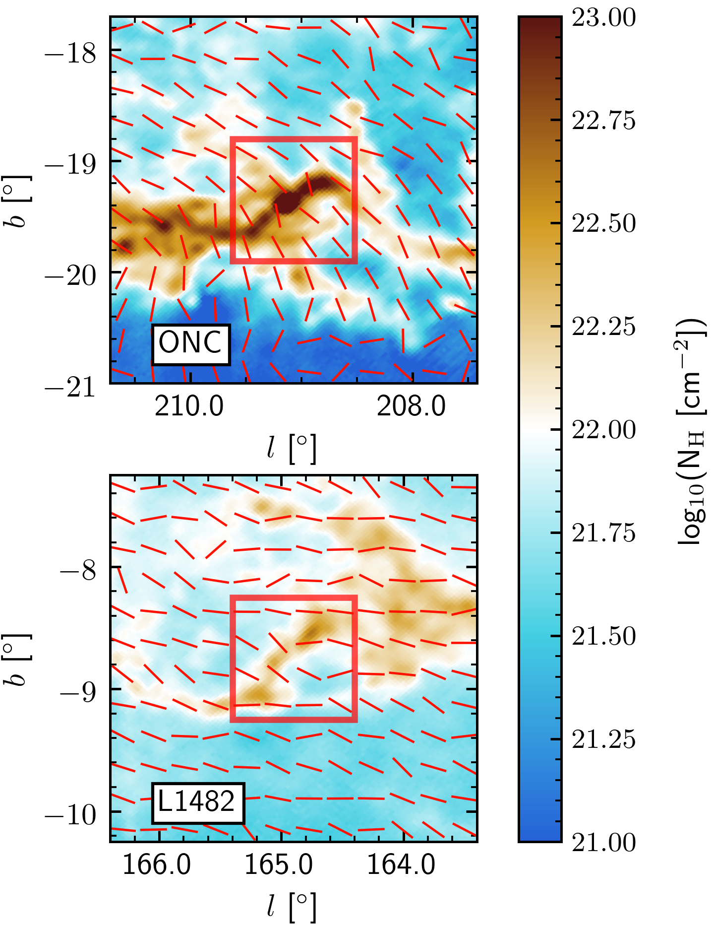
Figure 15: Planck $N_{\rm H}$ map (background) of the Orion ONC (top) and L1482 (bottom), both regions highlighted with red boxes. Red lines show the polarization vectors rotated by 90^∘ to indicate the orientation of the magnetic field projected on the plane of the sky. For both the ONC and L1482, the projected magnetic field is perpendicular to the filaments.

A velocity feature similar to that measured in L1482 has been studied in the Orion A ISF, reported by González Lobos & Stutz (2019) (and references therein) which they interpret as rotation. Based primarily on ¹²CO position-velocity (PV) diagrams, they identify two velocity components in the northern half of the ISF (see their Figure 8 and § 4.4) with estimated mean spatial separations of $\sim 1.3$ pc and angular velocities (assuming circular rotation) of $\sim 1.4$ Myr^-1. On smaller scales, they also present N₂H⁺ “bumps and wiggles” (see their Figure 4) that appear consistent with torsional-type structures with short timescales. While the relation between the larger ¹²CO and smaller scale N₂H⁺ velocity features in Orion A is not presently understood, they both present the appearance of rotational structures. The features that we characterize here in L1482, in contrast, are found in a lower density filament (see Figure 7), are closer to the central axis of the filament (the $N_{\rm H}$ ridgeline) than the ¹²CO Orion velocity feature, and may present different inner-filament timescales.

In terms of the magnetic field as probed by linear polarization, we can compare L1482, Orion, and G035. In G035 the projected magnetic field orientation presented by Liu et al. (2018) in the central portion “M” (high density) is perpendicular to the filament. The north and south portions (lower density) show a magnetic field almost parallel to the filament. This trend has been studied in multiple systems, including L1482 and the Orion A Integral Shaped Filament (ISF) region, containing the ONC. In Figure 15 we show the Planck polarization data (Planck Collaboration et al., 2014), which exhibits a projected field orientation that is preferentially perpendicular to the main filament axis (e.g., Soler, 2019; Planck Collaboration et al., 2016; Li et al., 2015; Tahani et al., 2018). The magnetic field morphology can be interpreted in 3D as either helical or bow-like (e.g., Inoue et al., 2018; Li & Klein, 2019; Tahani et al., 2018, 2019; Gómez et al., 2018). Moreover, close inspection of Figure 9 reveals that the northern portion of L1482-South has more prominent blue-shifted velocities, while the southern portion has more prominent red-shifted velocities, a signature that may be consistent with a helical velocity field in a filament with a 3D morphology similar to a corkscrew. One key question here is if the filament rotational motions may be linked to the 3D structure of the magnetic field in these systems, as seen for example in L1641 (Uchida et al., 1991). The combination of rotational motion about the long axis and a helical, or possibly bow–like (but see below), magnetic field morphology may be the most natural explanation that accounts for the combination of the observed gas radial velocities, the linear polarization patterns, and the overall “zig-zag” morphology of the filament. As discussed above, we suggest that future modeling of molecular line emission under various assumptions for the 3D density, velocity, and magnetic field properties would shed light on the structures we observe (e.g., Reissl et al., 2018a, b) and potentially yield constraints on the pitch-angle of the magnetic field in this system.

In terms of simulations, we find none, to the best of our knowledge, that reproduce rotational signatures similar to the ones we observe. In simulated turbulence and gravity-driven filament formation (e.g., Priestley & Whitworth, 2020), even when including magnetic fields (e.g., Gómez et al., 2018; Federrath, 2016; Li & Klein, 2019; Körtgen et al., 2017; Seifried et al., 2020; Wareing et al., 2020), rotation is not present. Moreover, these simulations probe low mass- and mass-per-unit-length scales compared to $\sim 10^{5}$ M_⊙ clouds and their correspondingly higher M/L filaments like California and Orion (see Table 3). See also Reissl et al. (2020) for a direct comparison between the line mass profiles in Orion and California/L1482 compared to one example of an MHD simulation of a filament.

Moreover, Inoue et al. (2018) and Li & Klein (2019) simulate somewhat higher mass clouds or regions, including models for magnetic fields. Li & Klein (2019) illustrate how the bow-shaped B-field morphology, in particular the directional flip on either side of the filament, is also consistent with the signature of a helical field along specific sight-lines (see their Figure 16). While they do not analyze the kinematics of the dense gas in detail, required for comparison to the specific signature presented here, they do detect a simulated flip in the velocity field on either side of the filament along certain sight-lines. Furthermore, their simulated filament is mostly very straight along its extent, exhibiting only slight, gentle curvature and not the “zig-zag” morphology that we observe here. Inoue et al. (2018) simulate the collapse in a small ($r=1.5$ pc) but massive ($M=838$ M_⊙) region. Their simulation produces a more massive sink particle ($M\gtrsim 50$ M_⊙) on a extremely short timescale of $\sim\,0.45$ Myr. Taking cuts across the sink particle, they recover some simulated velocity gradient; however, we observe no such analogies to massive sink particles (presumably these would be massive and very compact “clumps”). On the contrary, we have shown that our observations are consistent with a relatively smooth mass distribution along L1482-South. In summary, the detection in simulations of features resembling velocity gradients are an intriguing possibility for explaining the basic velocity flip that we detect; however we must not only explain this flip, but also the magnitude compared to gravity, the outer break and transition to shallower gradients, and the basic filament properties. Furthermore, these models require viewing the simulated filaments at specific angles in order to be consistent with the data and reproduce flips about the ridgelines, which may be reasonable for randomly oriented sets of filaments. However, the Gaia data (although this is not a strong constraint at present) would seem to imply that overall L1482, on larger scales, is not strongly inclined.

Meanwhile, lower density cosmological simulations also produce non-rotating filaments that arise due to the action of gravity (e.g. Springel et al., 2018). This is consistent with the idea that gravo-turbulent filaments simply do not rotate. In terms of observations, the situation is less clear but the existing data point toward a scenario where rotation appears not to be found in filaments in lower mass clouds (e.g., Hacar et al., 2016, 2013; Kirk et al., 2013; Shimajiri et al., 2019) but was analyzed for example in the high mass Orion A L1641 filament (Uchida et al., 1991). In particular, in Shimajiri et al. (2019), they study the velocity gradients in the Taurus B211/B213 in ¹²CO and ¹³CO (1-0). These authors interpret their velocity data with a model composed of two intersecting lower density sheets, observed at a specific viewing angle, and conclude that this particular system is well-reproduced by this configuration. They also note that because their tracers are optically thick, they require optically thin dense gas tracers to probe the velocity field inside the filament. As noted above, this is a straight filament, it is a lower mass and lower line-mass system: the Taurus B213 has an line mass of $\lambda_{app}\sim 100$ M_⊙/pc at a projected radius of $r\sim 1$ pc, about a factor of 2 lower than our measured $\lambda_{app}=205$ M_⊙/pc measured at the same projected radius of $r=1$ pc (see Table 3). The morphologies of the two filaments are very dissimilar, one being straight and mildly curved, while the L1482-South filament has a plane-of-the-sky “zig-zag” morphology.

Gradients have also been observed and quantified in other low mass regions, such as Serpens-Main (e.g. Olmi & Testi, 2002; Lee et al., 2014), using optically thin and high density gas tracers. In particular, Lee et al. (2014) observe a perpendicular gradient in the “FC1” filament in N₂H⁺, with an apparently sharp velocity jump. However, their main focus was the gradient along the filaments, and they do not suggest a physical origin for the perpendicular velocity gradients. In Serpens-South, a cloud assumed to be associated with Serpens-Main, Fernández-López et al. (2014) find perpendicular gradients in N₂H⁺ for filament “FE” (11.9 km s^-1 pc^-1) and “NFW”, but also dot not compare the velocity gradients to gravity. They postulate that the origin of these gradients is accretion from the local filament environment, and a result of projection in a flat structure that is inclined. In order to quantify how these gradients and their timescales compare with gravity and the L1482 filament, we suggest they should be revisited in combination with M/L profiles, similarly to the method we present in this paper. We also note that the simulations outlined above, and the low line-mass filaments analyzed in these observational studies, do not exhibit the two-dimensional “zig-zag” morphology that we observe in L1482. However, see Wareing et al. (2020) (in particular their Figure 6) for simulated filaments with ”wiggles” which may be comparable to the ”zig-zag” structure we observe. However, the Wareing et al. (2020) numerical experiments do not reveal rotation, emphasizing the importance of a comparison to all observational constraints presented here, and in particular the kinematic signatures presented in Figure 13.

Moreover, the lack of alignment between YSO outflows and filament orientation reported in Perseus (Stephens et al., 2017) may be consistent with the idea that lower mass clouds have more elevated levels of turbulent (and thus randomized velocity) support compared to higher mass clouds, as suggested by Stutz & Gould (2016). In contrast to Perseus, Kong et al. (2019) report the detection of filament-outflow orientation anti-correlation in the massive (M $\sim 10^{5}~{}\hbox{M${}_{\odot}$}$) G28.37$+$0.07 cloud. This may support the view presented in Stutz & Gould (2016) that the internal evolution of high mass clouds may be qualitatively different than low mass ones, specifically in relation to the role of rotation and the magnetic field in the collapse process.

Given the lack of rotation in lower mass turbulence simulations and lower mass clouds, the observations we present here would then lead to the suggestion that there must be some other mechanism for filament rotation in higher mass clouds. As mentioned above, the magnetic field is the only agent capable of playing this role (see e.g., Hennebelle, 2018; Schleicher & Stutz, 2018, and references therein). It may potentially act via magnetic breaking (by analogy to stars). This would imply that all filaments that are rotating must remove inner angular momentum via the magnetic field in order to collapse. The magnetic field would transport this rotational energy from small scales near the filament spines to larger radii. The observation of the more evolved L1482-North filament within this same cloud and just to the north, with fragmentation, accompanying protostar formation and no clear rotational signature, may support this idea of filament evolution. On the other hand, if the rotational signature is an imprint set by the earlier and diffuse ISM phase of cloud evolution, the question remains as to why lower mass clouds and their lower line-mass but still star-forming filaments are not rotating. Either the filaments where never rotating, which could be related to their mass-scale as suggested here, or observations and simulations should be able to capture an earlier lower-density phase of angular momentum dissipation.

We speculate that the structures reminiscent of helical or double helix loops seen here (see Figure 10), in Orion A (González Lobos & Stutz, 2019) and possibly to be seen in the G28.37$+$0.07 cloud (Kong et al., 2019), are the anchors of the magnetic fields. In this case, these would also be inevitable features of massive star forming filaments. If correct, this would make magnetic fields an essential feature of (massive) star and cluster forming filaments. Linking the rotational signatures to the magnetic field naturally leads to a torsional, helical, or bow–like field morphology. The observed velocity flip perpendicular to the L1482-South ridgeline (Figure 9) is also accompanied by a flip in the magnetic field (Tahani et al., 2018) in California on larger scales, a flip that these authors interpreted as a possible signature of magnetic field helicity. The connection between the large-scale inferred field geometry and the small scale velocity feature we detect is not presently understood and must be investigated in future work.

8 Conclusions

Previous studies have shown that the California molecular cloud is similar to Orion A in terms of mass (M $\sim 10^{5}$ M_⊙), morphology, undulating filaments, and magnetic field geometry but strikingly different in YSO content (Lada et al., 2009; Megeath et al., 2012; Kong et al., 2015; Lada et al., 2017; Tahani et al., 2018). We present the study of the filament L1482 located in California. L1482 is one of the most massive filaments in California and contains $\sim$ 56% of the YSOs in the cloud. Here we characterize the physical properties of this filament by combining the analysis of YSO distance information, gas mass distributions, and gas velocities. We summarize our main results as follows.
$\bullet$ We find a distance of 511${}^{+17}_{-16}$ pc based on Gaia DR2 astrometry of YSOs in the filament.
$\bullet$ Using Herschel and Planck $N_{\rm H}$ maps, we characterize the projected mass per unit length (M/L) of the L1482 filament as a whole, and divide the filament into two distinct regions based on differences in the presence of star formation, M/L profiles, morphology, and gas velocities (see below): the South, with a lower M/L, no star formation, a plane-of-the-sky “zig-zag” morphology, and coherent velocity patterns, versus the North, with star formation, a higher M/L profile, and more chaotic velocity patterns.
$\bullet$ All the above regions of the filament have M/L profiles consistent with a scale-free power-law shape. At 1 pc, the filament as a whole, the North, and the South regions have M/L power-law normalizations of 214, 264, and 205 $\hbox{M${}_{\odot}$}\rm{pc}^{-1}$ and power-law indices of 0.62, 0.51, and 0.64, respectively. See Table 3 and Figure 7 for full M/L profiles.
$\bullet$ Based on the M/L profiles, and assuming cylindrical geometry and axial symmetry motivated by the mass distribution (see Figures 6 & 7), we calculate the volume density, gravitational potential, and gravitational acceleration profiles. See Table 3.
$\bullet$ We present intensity-weighted position-velocity diagrams of IRAM 30 m observations of C¹⁸O, HCO⁺, HNC, and N₂H⁺ (1-0). These reveal complex twisting and turning velocity structures, with timescales of order $\sim\,1$ Myr. These undulations are particularly striking in the South of L1482 in C¹⁸O.
$\bullet$ We detect a velocity profile in C¹⁸O consistent with rotation about the long-axis of the South filament. The velocity profile pattern is regular and smooth. It profile “hugs” the filament, that is, it is confined to within $r\lesssim\pm 0.4$ pc from the $N_{\rm H}$ ridgeline and is anti-symmetric about the ridgeline. See Figure 13.
$\bullet$ The above velocity profile grows linearly to $r~{}\sim~{}0.25$ pc, outside of which it softens to shallower slope. The inner ($r~{}\leq~{}0.25$ pc) timescale of the velocity gradient is 0.7 Myr. The outer ($r~{}>~{}0.25$ pc) timescale is much longer, about 6 Myr.
$\bullet$ When compared to the gravitational field, and using a simple solid body rotation toy model, the rotational profile implies that the filament approaches break-up at $r\sim 0.25$ pc, where it transitions to being gravity-regulated. See Figure 14.
$\bullet$ The long timescales on the outside of the rotational profile, combined with the break in the rotational profile, imply that the filament structure is stable and long lived (few times 6 Myr) and that the filament is undergoing outside-in evolution in the process of dissipating its angular momentum toward collapse and eventual star formation (as is observed in the North portion of the larger L1482 filamentary structure).
$\bullet$ The above results assume the filament is oriented in the plane of the sky. While the filament inclination is not well-constrained, the role of rotation compared to gravity will only be greater if the inclination is non-zero.
$\bullet$ The Planck polarization vectors, rotated to infer the plane-of-the-sky magnetic field geometry, are approximately perpendicular to the to main filament axis, as is also seen in other clouds such as Orion A and in G035. The appearance of the position-velocity diagrams, the rotational signature discussed above, and the plane-of-the-sky “zig-zag” morphology of the filament, taken together with Planck, may imply a 3D “corkscrew” filament with a helical magnetic field morphology could be a natural explanation of the various observational constraints. Meanwhile, a “bow” shaped field (as reproduced in simulations) may also account for certain observational features, such as the flip in the magnetic field along the line-of-sight and the magnetic field in the POS being perpendicular to the filament.

Comparison to turbulence and MHD simulations (which do not show rotation in filaments), observations of lower mass filaments (which also do not show rotation, see the related discussion in § 7), previous results in Orion A, constraints from e.g., the G035 filament, together lead to the suggestion that high mass (M $\sim 10^{5}$ M_⊙) clouds host rotating filaments that may be more common than previously thought. In this hypothesis, these structures must undergo angular momentum evolution (e.g., Hennebelle 2018 and references therein), for example losing angular momentum through rotation, in order to collapse as they progress toward star cluster formation.

We speculate that the observed velocity flip across the filament on small scales may be related to the flip in the magnetic field observed in California on far larger scales (Tahani et al., 2018). We emphasize that the connection between the large scale signatures of field geometry and the small scale velocity features detected here are not presently understood. Hence, further investigation into the scale dependence of the magnetic field strengths and geometries are essential. Moreover, future observational work should include scrutiny of larger portions of California to more broadly characterize the gas kinematics. Wide-field observations that trace magnetic fields on filament scales (capturing scales of $\lesssim$0.1 pc to $\gtrsim$10 pc and cloud scales, including Zeeman when possible, are essential for obtaining further constraints on both field geometry and strength. Constraining gas kinematics in combination with constraints for the magnetic field is critical. Scrutiny of the YSO and stellar kinematics, including radial velocities, and their possible link to the cloud kinematics, will explore the link between the stellar and gas content (Stutz & Gould, 2016). Besides California and Orion A, it is imperative to kinematically characterize other high-mass filaments like e.g., G28.37$+$0.07 (Kong et al., 2019). Finally, numerical work should focus on molecular line modeling of the velocity field of ”zig-zag” filaments to elucidate the 3D structure filaments that have a significant degree of rotation (see e.g., Reissl et al., 2018a, b).

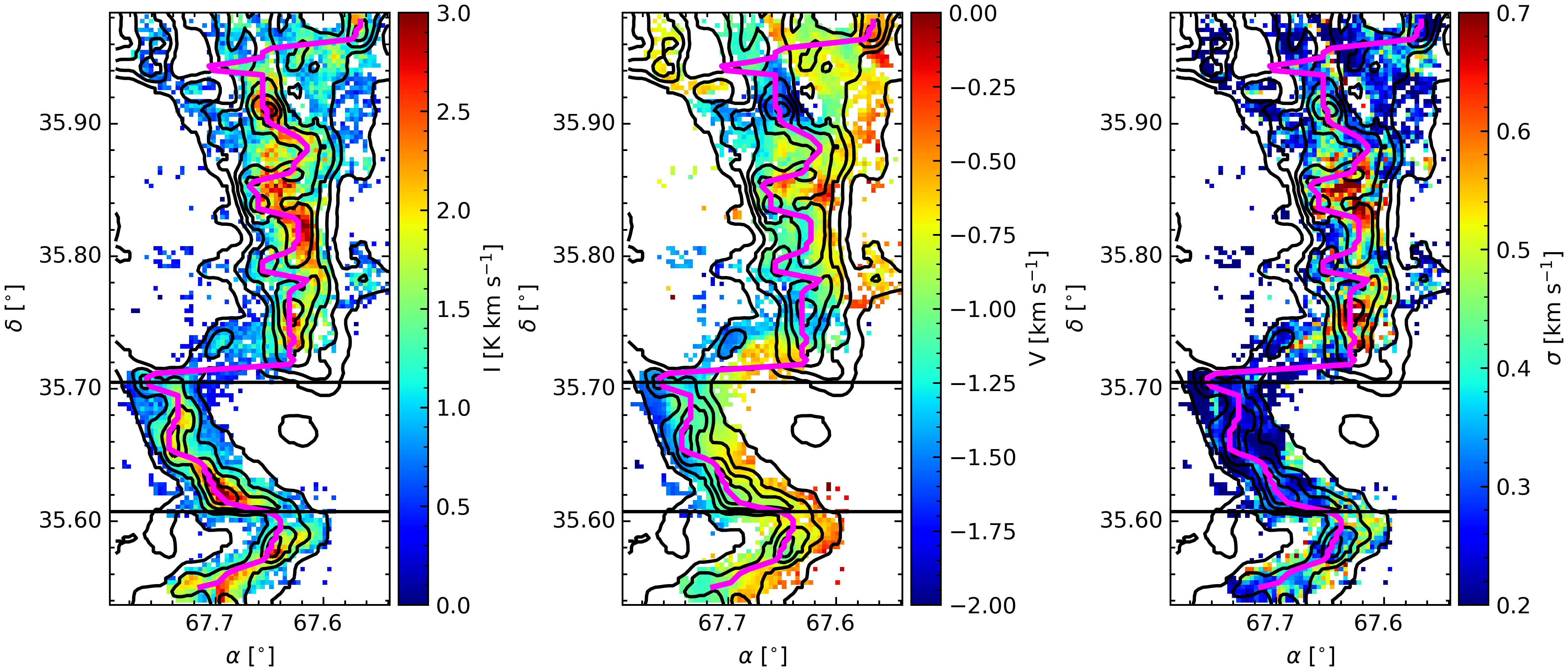
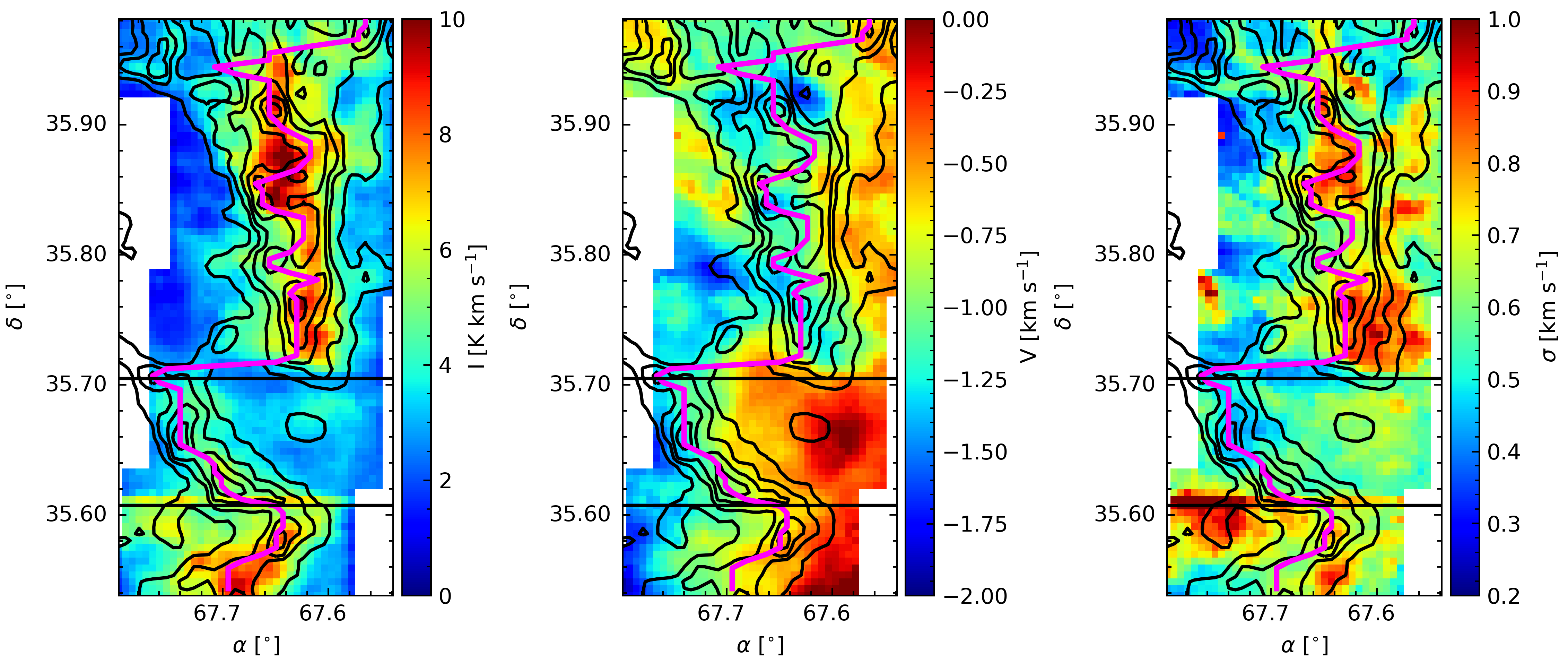
Figure A.1: C¹⁸O (top) and ¹³CO (bottom) moments 0, 1, and 2 maps (left to right, respectively). The horizontal black lines indicate the extent of the South region (see text). The magenta curve indicates the $N_{\rm H}$ ridgeline. The black contours follow $log_{10}(N_{\rm H}/\rm{cm}^{-2})=21.9,22.1,22.3,22.4,22.6$, and $22.8$ values from the Herschel maps.

Appendix A Moment maps

In Figure A.1 we show the first 3 moment maps (from left to right) for C¹⁸O (top) and ¹³CO (bottom). These figures show that the filament is well traced in C¹⁸O, but less so in ¹³CO, a fact that is particularly obvious in the velocity and line width (moments 1 and 2) maps.

We find a larger scale ¹³CO gradient in the same region we are analyzing. It is tempting to associate the ¹³CO gradient with the C¹⁸O gradient, but as the moment maps show, the ¹³CO tracer is simply not isolating the filament structure (including the radial velocities) nearly as well as the C¹⁸O. For example, the filament is barely detected in the ¹³CO moments 1 and 2 maps, and is only marginally detected in the moment 0 map; moreover the ¹³CO gradient (not shown) is of a different magnitude as the C¹⁸O, likely because the ¹³CO is simply not tracing the filament but instead the broader and less well defined cloud environment. Moreover, the rotational signature seen in Figure 13 is not observed in the immediately adjacent North region, as can be appreciated from the moment maps. This is consistent with our interpretation that in the North gravity has already take over, as evidenced by the protostar content. In summary, other lower density and optically thick tracers are simply inadequate for isolating the filament and its velocities.

Appendix B Temperature profile

In Figure B.1 we show the average projected radial temperature profile (black solid line) of CMC/L1482. We calculate this profile following the ridgeline (see above). We also present the east and west temperature profiles. Inside the radial range where the profile is used (see § 5.3), that is at r $\lesssim 1$ pc, the profile is approximately symmetric and variations are small. Therefore we fit the average temperature profile with a softened power-law (red solid line). We obtain the following best-fit temperature profile:

$$\rm{T}(r) = 12.3\ (1+(r/a)^{2})^{0.04}\,\rm{K};\qquad\textit{a}=0.9~{}{\rm pc}.$$ (B1)

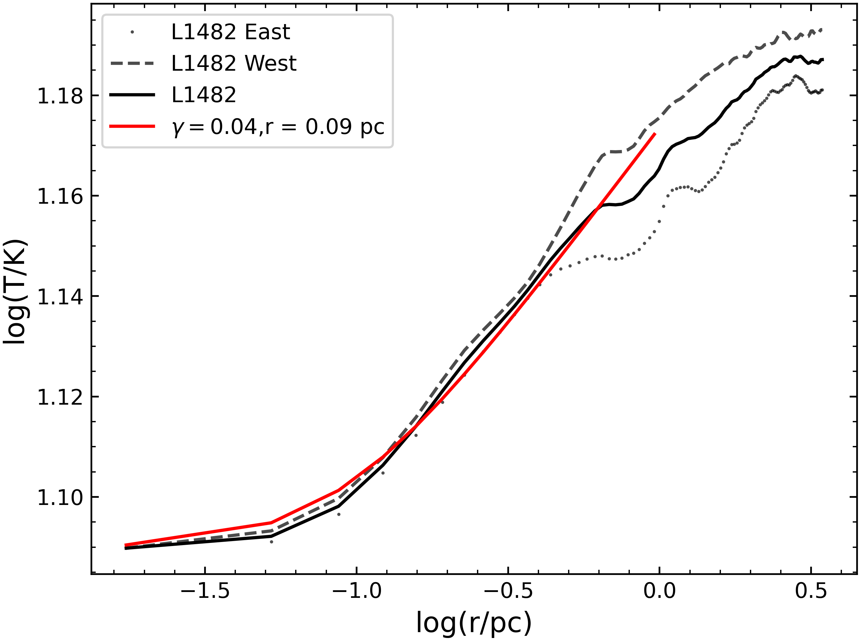
Figure B.1: Average CMC/L1482 temperature profile derived from the Herschel temperature map (black solid line). Dotted (dashed) curve corresponds to the east (west) profile. The profiles are highly symmetric over the inner width of the filament. The red curve shows the best-fit (see Eq. B1) to the solid black line, and is plotted over the radial range that it is used in §5.3 and in Figure 12.

References

- Abreu-Vicente et al. (2017) Abreu-Vicente, J., Stutz, A., Henning, T., et al. 2017, A&A, 604, A65
- Andrews & Wolk (2008) Andrews, S. M., & Wolk, S. J. 2008, The LkH 101 Cluster, ed. B. Reipurth, Vol. 4, 390
- Arenou et al. (2018) Arenou, F., Luri, X., Babusiaux, C., et al. 2018, A&A, 616, A17
- Caselli et al. (2002) Caselli, P., Benson, P. J., Myers, P. C., & Tafalla, M. 2002, ApJ, 572, 238
- Choi et al. (2020) Choi, S. K., Austermann, J., Basu, K., et al. 2020, Journal of Low Temperature Physics, 199, 1089
- Contreras et al. (2013) Contreras, Y., Rathborne, J., & Garay, G. 2013, MNRAS, 433, 251
- Dame et al. (2001) Dame, T. M., Hartmann, D., & Thaddeus, P. 2001, ApJ, 547, 792
- Evans et al. (2015) Evans, Neal J., I., Di Francesco, J., Lee, J.-E., et al. 2015, ApJ, 814, 22
- Falgarone et al. (2001) Falgarone, E., Pety, J., & Phillips, T. G. 2001, ApJ, 555, 178
- Federrath (2016) Federrath, C. 2016, MNRAS, 457, 375
- Fernández-López et al. (2014) Fernández-López, M., Arce, H. G., Looney, L., et al. 2014, ApJ, 790, L19
- Fiege & Pudritz (2000a) Fiege, J. D., & Pudritz, R. E. 2000a, MNRAS, 311, 85
- Fiege & Pudritz (2000b) —. 2000b, MNRAS, 311, 105
- Fischer et al. (2017) Fischer, W. J., Megeath, S. T., Furlan, E., et al. 2017, ApJ, 840, 69
- Fukui et al. (2018) Fukui, Y., Torii, K., Hattori, Y., et al. 2018, ApJ, 859, 166
- Gaia Collaboration et al. (2018a) Gaia Collaboration, Babusiaux, C., van Leeuwen, F., et al. 2018a, A&A, 616, A10
- Gaia Collaboration et al. (2018b) Gaia Collaboration, Brown, A. G. A., Vallenari, A., et al. 2018b, A&A, 616, A1
- Ginsburg & Mirocha (2011) Ginsburg, A., & Mirocha, J. 2011, PySpecKit: Python Spectroscopic Toolkit, Astrophysics Source Code Library, ascl:1109.001
- Gómez & Vázquez-Semadeni (2014) Gómez, G. C., & Vázquez-Semadeni, E. 2014, ApJ, 791, 124
- Gómez et al. (2018) Gómez, G. C., Vázquez-Semadeni, E., & Zamora-Avilés, M. 2018, MNRAS, 480, 2939
- González Lobos & Stutz (2019) González Lobos, V., & Stutz, A. M. 2019, MNRAS, 489, 4771
- Gould (2003) Gould, A. 2003, arXiv e-prints, astro
- Griffin et al. (2010) Griffin, M. J., Abergel, A., Abreu, A., et al. 2010, A&A, 518, L3
- Hacar et al. (2016) Hacar, A., Kainulainen, J., Tafalla, M., Beuther, H., & Alves, J. 2016, A&A, 587, A97
- Hacar et al. (2013) Hacar, A., Tafalla, M., Kauffmann, J., & Kovács, A. 2013, A&A, 554, A55
- Harvey et al. (2013) Harvey, P. M., Fallscheer, C., Ginsburg, A., et al. 2013, ApJ, 764, 133
- Heiles (1987) Heiles, C. 1987, Interstellar Magnetic Fields, ed. D. J. Hollenbach & J. Thronson, Harley A., Vol. 134, 171
- Heiles (1997) —. 1997, ApJS, 111, 245
- Hennebelle (2003) Hennebelle, P. 2003, A&A, 397, 381
- Hennebelle (2018) —. 2018, Astrophysics and Space Science Library, Vol. 424, Numerical Simulations of Cluster Formation, ed. S. Stahler, 39
- Henshaw et al. (2014) Henshaw, J. D., Caselli, P., Fontani, F., Jiménez-Serra, I., & Tan, J. C. 2014, MNRAS, 440, 2860
- Henshaw et al. (2013) Henshaw, J. D., Caselli, P., Fontani, F., et al. 2013, MNRAS, 428, 3425
- Herbig et al. (2004) Herbig, G. H., Andrews, S. M., & Dahm, S. E. 2004, AJ, 128, 1233
- Inoue et al. (2018) Inoue, T., Hennebelle, P., Fukui, Y., et al. 2018, PASJ, 70, S53
- Jiménez-Serra et al. (2014) Jiménez-Serra, I., Caselli, P., Fontani, F., et al. 2014, MNRAS, 439, 1996
- Kainulainen & Tan (2013) Kainulainen, J., & Tan, J. C. 2013, A&A, 549, A53
- Kirk et al. (2013) Kirk, H., Myers, P. C., Bourke, T. L., et al. 2013, ApJ, 766, 115
- Kong et al. (2019) Kong, S., Arce, H. G., Maureira, M. J., et al. 2019, ApJ, 874, 104
- Kong et al. (2015) Kong, S., Lada, C. J., Lada, E. A., et al. 2015, ApJ, 805, 58
- Körtgen et al. (2017) Körtgen, B., Federrath, C., & Banerjee, R. 2017, MNRAS, 472, 2496
- Lada et al. (2017) Lada, C. J., Lewis, J. A., Lombardi, M., & Alves, J. 2017, A&A, 606, A100
- Lada et al. (2009) Lada, C. J., Lombardi, M., & Alves, J. F. 2009, ApJ, 703, 52
- Lada et al. (2010) —. 2010, ApJ, 724, 687
- Launhardt et al. (2013) Launhardt, R., Stutz, A. M., Schmiedeke, A., et al. 2013, A&A, 551, A98
- Law et al. (2020) Law, C. Y., Li, H. B., Cao, Z., & Ng, C. Y. 2020, MNRAS, 498, 850
- Law et al. (2019) Law, C. Y., Li, H. B., & Leung, P. K. 2019, MNRAS, 484, 3604
- Lee et al. (2014) Lee, K. I., Fernández-López, M., Storm, S., et al. 2014, ApJ, 797, 76
- Li et al. (2014) Li, D. L., Esimbek, J., Zhou, J. J., et al. 2014, A&A, 567, A10
- Li et al. (2015) Li, H.-B., Yuen, K. H., Otto, F., et al. 2015, Nature, 520, 518
- Li & Klein (2019) Li, P. S., & Klein, R. I. 2019, MNRAS, 485, 4509
- Lindegren et al. (2018) Lindegren, L., Hernández, J., Bombrun, A., et al. 2018, A&A, 616, A2
- Lippok et al. (2013) Lippok, N., Launhardt, R., Semenov, D., et al. 2013, A&A, 560, A41
- Liu et al. (2019) Liu, H.-L., Stutz, A., & Yuan, J.-H. 2019, MNRAS, 487, 1259
- Liu et al. (2018) Liu, T., Li, P. S., Juvela, M., et al. 2018, ApJ, 859, 151
- Lombardi et al. (2014) Lombardi, M., Bouy, H., Alves, J., & Lada, C. J. 2014, A&A, 566, A45
- Matthews & Wilson (2000) Matthews, B. C., & Wilson, C. D. 2000, ApJ, 531, 868
- Megeath et al. (2012) Megeath, S. T., Gutermuth, R., Muzerolle, J., et al. 2012, AJ, 144, 192
- Miville-Deschênes et al. (2017) Miville-Deschênes, M.-A., Murray, N., & Lee, E. J. 2017, ApJ, 834, 57
- Motte et al. (2018) Motte, F., Bontemps, S., & Louvet, F. 2018, ARA&A, 56, 41
- Myers et al. (2000) Myers, P. C., Evans, N. J., I., & Ohashi, N. 2000, in Protostars and Planets IV, ed. V. Mannings, A. P. Boss, & S. S. Russell, 217
- Nguyen Luong et al. (2011) Nguyen Luong, Q., Motte, F., Hennemann, M., et al. 2011, A&A, 535, A76
- Olmi & Testi (2002) Olmi, L., & Testi, L. 2002, A&A, 392, 1053
- Ossenkopf & Henning (1994) Ossenkopf, V., & Henning, T. 1994, A&A, 291, 943
- Penoyre et al. (2020) Penoyre, Z., Belokurov, V., Wyn Evans, N., Everall, A., & Koposov, S. E. 2020, MNRAS, 495, 321
- Planck Collaboration et al. (2014) Planck Collaboration, Abergel, A., Ade, P. A. R., et al. 2014, A&A, 571, A11
- Planck Collaboration et al. (2016) Planck Collaboration, Ade, P. A. R., Aghanim, N., et al. 2016, A&A, 586, A138
- Poglitsch et al. (2010) Poglitsch, A., Waelkens, C., Geis, N., et al. 2010, A&A, 518, L2
- Priestley & Whitworth (2020) Priestley, F. D., & Whitworth, A. P. 2020, MNRAS, 499, 3728
- Rao et al. (2020) Rao, A., Gandhi, P., Knigge, C., et al. 2020, MNRAS, 495, 1491
- Reissl et al. (2018a) Reissl, S., Stutz, A. M., Brauer, R., et al. 2018a, MNRAS, 481, 2507
- Reissl et al. (2020) Reissl, S., Stutz, A. M., Klessen, R. S., Seifried, D., & Walch, S. 2020, arXiv e-prints, arXiv:2009.04201
- Reissl et al. (2018b) Reissl, S., Wolf, S., & Brauer, R. 2018b, POLARIS: POLArized RadIation Simulator, ascl:1807.001
- Schleicher & Stutz (2018) Schleicher, D. R. G., & Stutz, A. 2018, MNRAS, 475, 121
- Seifried et al. (2020) Seifried, D., Haid, S., Walch, S., Borchert, E. M. A., & Bisbas, T. G. 2020, MNRAS, 492, 1465
- Shimajiri et al. (2019) Shimajiri, Y., André, P., Palmeirim, P., et al. 2019, A&A, 623, A16
- Simon et al. (2006) Simon, R., Rathborne, J. M., Shah, R. Y., Jackson, J. M., & Chambers, E. T. 2006, ApJ, 653, 1325
- Smith et al. (2012) Smith, R. J., Shetty, R., Stutz, A. M., & Klessen, R. S. 2012, ApJ, 750, 64
- Sodroski et al. (1997) Sodroski, T. J., Odegard, N., Arendt, R. G., et al. 1997, ApJ, 480, 173
- Soler (2019) Soler, J. D. 2019, A&A, 629, A96
- Springel et al. (2018) Springel, V., Pakmor, R., Pillepich, A., et al. 2018, MNRAS, 475, 676
- Stephens et al. (2017) Stephens, I. W., Dunham, M. M., Myers, P. C., et al. 2017, ApJ, 846, 16
- Stutz et al. (2010) Stutz, A., Launhardt, R., Linz, H., et al. 2010, A&A, 518, L87
- Stutz (2018) Stutz, A. M. 2018, MNRAS, 473, 4890
- Stutz et al. (2018) Stutz, A. M., Gonzalez-Lobos, V. I., & Gould, A. 2018, arXiv e-prints, arXiv:1807.11496
- Stutz & Gould (2016) Stutz, A. M., & Gould, A. 2016, A&A, 590, A2
- Stutz & Kainulainen (2015) Stutz, A. M., & Kainulainen, J. 2015, A&A, 577, L6
- Stutz et al. (2013) Stutz, A. M., Tobin, J. J., Stanke, T., et al. 2013, ApJ, 767, 36
- Tafalla et al. (2002) Tafalla, M., Myers, P. C., Caselli, P., Walmsley, C. M., & Comito, C. 2002, ApJ, 569, 815
- Tahani et al. (2018) Tahani, M., Plume, R., Brown, J. C., & Kainulainen, J. 2018, A&A, 614, A100
- Tahani et al. (2019) Tahani, M., Plume, R., Brown, J. C., Soler, J. D., & Kainulainen, J. 2019, A&A, 632, A68
- Terry et al. (2019) Terry, H., Battaglia, N., Basu, K., et al. 2019, in Bulletin of the American Astronomical Society, Vol. 51, 213
- Uchida et al. (1991) Uchida, Y., Fukui, Y., Minoshima, Y., Mizuno, A., & Iwata, T. 1991, Nature, 349, 140
- Ungerechts & Thaddeus (1987) Ungerechts, H., & Thaddeus, P. 1987, ApJS, 63, 645
- Wareing et al. (2020) Wareing, C. J., Pittard, J. M., & Falle, S. A. E. G. 2020, MNRAS, arXiv:2011.01321
- Zinn et al. (2019) Zinn, J. C., Pinsonneault, M. H., Huber, D., & Stello, D. 2019, ApJ, 878, 136
- Zucker et al. (2019) Zucker, C., Speagle, J. S., Schlafly, E. F., et al. 2019, ApJ, 879, 125