C³ - Cluster Clustering Cosmology
I. New constraints on the cosmic growth rate at $z\sim 0.3$ from redshift-space clustering anisotropies

Abstract

Redshift-space distortions in the clustering of galaxy clusters provide a novel probe to test the theory of gravity on cosmological scales. The aim of this work is to derive new constraints on the linear growth rate of cosmic structures from the redshift-space two-point correlation function of galaxy clusters. We construct a large spectroscopic catalog of optically-selected clusters from the Sloan Digital Sky Survey. The selected sample consists of $43,743$ clusters in the redshift range $0.1<z<0.42$, with masses estimated from weak-lensing calibrated scaling relations. We measure the transverse and radial wedges of the two-point correlation function of the selected clusters. Modeling the redshift-space clustering anisotropies, we provide the first constraints on the linear growth rate from cluster clustering. The cluster masses are used to set a prior on the linear bias of the sample. This represents the main advantage in using galaxy clusters as cosmic probes, instead of galaxies. Assuming a standard cosmological model consistent with the latest cosmic microwave background constraints, we do not find any evidence of deviations from general relativity. Specifically, we get the value of the growth rate times the matter power spectrum normalization parameter $f\sigma_{8}=0.44\pm 0.05$, at an effective redshift of $z=0.275$.

1 Introduction

The spatial distribution of matter in the universe depends on both the expansion rate of space and the peculiar velocities at small scales caused by local gravitational interactions. Second-order and third-order summary statistics of the matter density field, i.e. the two-point (2PCF) and three-point auto-correlation functions, provide key information on the main cosmological model parameters, and can be effectively assessed through the corresponding statistics of properly selected samples of biased cosmic tracers, such as galaxies. In particular, apparent anisotropies in the 2PCF, induced by neglecting the peculiar velocities along the line of sight when computing comoving distances, can be effectively exploited to test the gravity theory on the largest cosmological scales. Redshift-space distortions (RSD, Kaiser, 1987; Hamilton, 1998) in clustering statistics provide an indirect measurement of the properties of the matter peculiar velocity field, which can be parameterized by the linear growth rate of cosmic structures, $f\equiv d\log G/d\log a$, where $G$ is the growth factor and $a$ is the scale factor (Peacock et al., 2001; Hawkins et al., 2003; Guzzo et al., 2008; Zhang et al., 2008). Combining measurements of the cosmic growth rate and of the Hubble expansion rate it is possible to discriminate among alternative dark energy models (Linder, 2017; Moresco & Marulli, 2017).

Large and dense samples of extragalactic sources are required to accurately measure the 2PCF in a wide enough range of comoving coordinates and redshifts, at sufficiently high signal-to-noise ratio. Different tracers are generally considered to maximize the redshift range covered (e.g. Alam et al., 2021). Measurements from the auto- and cross-correlation functions of galaxies (e.g. Percival et al., 2004; Samushia et al., 2012, 2014; Tojeiro et al., 2012; Reid et al., 2012; Chuang & Wang, 2013; Chuang et al., 2013, 2016; Beutler et al., 2014; Okumura et al., 2016; de la Torre et al., 2017; Adams & Blake, 2017; Pezzotta et al., 2017; Mohammad et al., 2018; Icaza-Lizaola et al., 2020; Wang et al., 2020), quasars (e.g. Neveux et al., 2020; Hou et al., 2021), cosmic voids (e.g. Hamaus et al., 2016, 2020; Hawken et al., 2017, 2020; Nadathur et al., 2019, 2020; Aubert et al., 2020) and other probes (e.g. Davis et al., 2011; Turnbull et al., 2012; Hudson & Turnbull, 2012; Feix et al., 2015) allowed testing the gravity theory on a wide redshift range, up to $z\sim 1.5$ (see the discussion of our results in §5).

The goal of this work is to provide new constraints on the linear growth rate of cosmic structures from the redshift-space 2PCF of a large spectroscopic sample of galaxy clusters extracted from the Sloan Digital Sky Survey (SDSS), at an effective redshift $z\sim 0.3$. In Moresco et al. (2021) we analyze the three-point correlation function of the same catalog up to the baryon acoustic oscillations (BAO) scales and provide constraints on the nonlinear bias of the sample, while in Veropalumbo et al. (in prep.) we perform a joint RSD+BAO analysis of the two-point and three-point correlation functions.

Galaxy clusters are the biggest structures that are virialized in the present universe. Large-scale cluster statistics provide one of the primary probes to constrain the universe’s geometry and growth rate, especially because the masses of dark matter haloes hosting clusters can be accurately assessed via different techniques, exploiting the cluster multiwavelength signal. In particular, the redshift evolution of cluster number counts provides strong cosmological constraints on the total matter energy density parameter, $\Omega_{\rm M}$, and on the amplitude of the matter power spectrum, $\sigma_{8}$ (see e.g. Vikhlinin et al., 2009; Pacaud et al., 2018; Costanzi et al., 2019; Lesci et al., 2020, and references therein). The clustering of galaxy clusters is a harder statistics to measure, as it requires dense samples of sources in a wide comoving separation range. Nevertheless, the cluster 2PCF has already been deeply exploited in cosmological studies, also in combination with other cluster probes such as number counts and gravitational lensing (see e.g. Moscardini et al., 2000; Miller & Batuski, 2001; Schuecker et al., 2001, 2003; Majumdar & Mohr, 2004; Estrada et al., 2009; Hütsi, 2010; Balaguera-Antolínez et al., 2011; Hong et al., 2012, 2016; Mana et al., 2013; Veropalumbo et al., 2014, 2016; Sereno et al., 2015; Emami et al., 2017; Marulli et al., 2018; Nanni et al., in prep.).

In fact, cluster clustering offers several key advantages relative to galaxy clustering (e.g. Angulo et al., 2005; Marulli et al., 2017). Galaxy clusters are highly biased tracers; thus, at a given scale, their 2PCF clustering signal is high compared to galaxies, and increases with cluster masses (Sheth et al., 2001). Furthermore, pure enough galaxy cluster samples, with a negligible fraction of satellite galaxies erroneously identified as Brightest Cluster Galaxies (BCGs), are relatively less affected by nonlinear dynamics at small scales – the so-called Fingers-of-God distortions, which reduces the impact of possible systematics from RSD model assumptions (Valageas & Clerc, 2012; Marulli et al., 2017). Large spectroscopic cluster catalogs have also been proven to be optimal probes for BAO cosmological analyses, due to low damping in the BAO shape as compared to galaxy clustering (Hong et al., 2012, 2016; Veropalumbo et al., 2014, 2016). On the other hand, high-mass cluster-scale haloes are known to exhibit nonlinear bias (see e.g. Desjacques et al., 2018) which should be properly modeled in the likelihood function, as discussed in §4.1. Finally, as mentioned before, another key benefit of using clusters as cosmological probes is the possibility of assessing cluster masses, which can be used in cluster clustering analyses to estimate the effective bias of the sample when a cosmological model is assumed. Furthermore, the cosmological dependence of cluster mass estimates might be exploited to further strengthen the cosmological constraints.

Throughout this paper we assume a fiducial $\Lambda$-cold dark matter ($\Lambda$CDM) cosmological model consistent with Planck Collaboration et al. (2020, Planck18) parameters, i.e. $\Omega_{M}=0.3153$, $\Omega_{\Lambda}=0.6846$, $\Omega_{b}=0.0486$, $\sigma_{8}=0.8111$, $n_{s}=0.9649$. The dependence of observed coordinates on the Hubble parameter is expressed as a function of $h\equiv H_{0}/100\,{\rm km\,s^{-1}Mpc^{-1}}$.

The analyses presented in this work have been performed with the CosmoBolognaLib (Marulli et al., 2016), a set of free software numerical libraries that we used here to handle the catalog of galaxy clusters, measure their clustering statistics, and perform Bayesian statistical analyses aimed at extracting constraints from redshift-space clustering anisotropies.

The paper is organized as follows. In §2 we present the spectroscopic cluster sample used in this work, describing the selection criteria and cluster main properties. In §3 and §4 we explain the adopted methods and assumptions to measure and model the redshift-space clustering wedges, respectively. The results of the analysis are presented and discussed in §5, while §6 summarizes the main findings of this work.

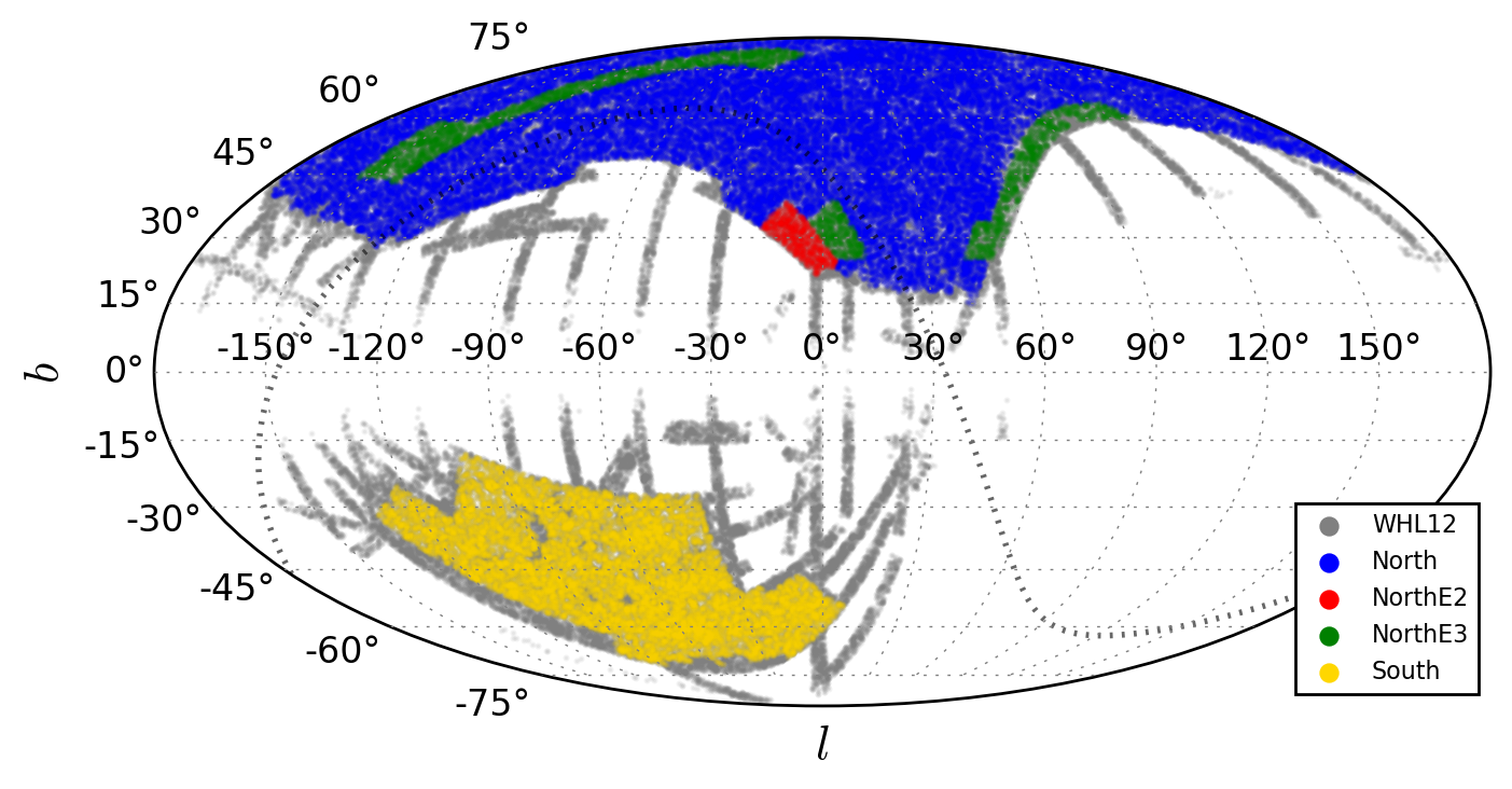
Figure 1: The angular distribution of the spectroscopic cluster sample analyzed in this work, in the north (blue points), north E2 (red points), north E3 (green points) and south (yellow points) fields, compared to the WHL12 photometric sample (gray points, in background). The map is shown in the Galactic Coordinate System. The dotted black line indicates the Celestial Equator.

2 The data

2.1 The photometric sample

The catalog analyzed in this work consists of optically selected clusters of galaxies that have been identified by Wen et al. (2012, WHL12) from the Sloan Digital Sky Survey III (Aihara et al., 2011, SDSS-III, Data Release (DR) 8).

The WHL12 catalog lists $132,684$ galaxy clusters on a sky area of $\sim 15,000$ square degrees, spanning the redshift range $0.05<z<0.8$. The cluster identification is based on a friends-of-friends procedure (Huchra & Geller, 1982). This approach has been already exploited to find groups and clusters using volume-limited spectroscopic samples of galaxies (see e.g. Berlind et al., 2006; Tempel et al., 2014) at low redshifts ($z<0.2$). The WHL12 cluster sample extends the technique on photometric redshift samples of galaxies, allowing the detection of galaxy overdensities around the BCGs at higher redshifts.

A candidate cluster is included in the catalog if $N_{200}\geq 8$ and $R_{L_{*}}\geq 12$, where $N_{200}$ is the number of member candidates within $\tilde{r}_{200}$, and $R_{L_{*}}$ is the optical richness defined as $R_{L_{*}}=\tilde{L}_{200}/L_{*}$, where $\tilde{L}_{200}$ is the total $r$-band luminosity within an empirically determined radius $\tilde{r}_{200}$ and $L_{*}$ is the evolved characteristic galaxy luminosity (Blanton et al., 2003). The subscript $200$ denotes quantities measured in a sphere whose mean density is $200$ times the critical density at the cluster redshift. The cluster photometric redshifts reported in the catalog are the median value of the photometric redshifts of the galaxy members. These selections have been applied to avoid contaminations by bright field galaxies with overestimated photometric redshifts.

The cluster masses are estimated from the weak-lensing cluster mass scaling relation calibrated in WHL12, with data from Wen et al. (2010):

$$\log\left(\frac{M_{200}}{10^{14}M_{\odot}}\right)=(-1.49\pm 0.05)+(1.17\pm 0.03)\log\left(R_{L_{*}}\right)\,.$$ (1)

To verify the robustness of our analysis, we consider also the scaling relation provided independently by Covone et al. (2014), finding consistent results.

According to WHL12, the catalog completeness, which is the fraction of the selected galaxy clusters over the full sample, is close to $1$ in the redshift range $0.1<z<0.42$, for $M_{200}\gtrsim 2\times 10^{14}M_{\odot}$, while the detection rate decreases down to $\sim 75\%$, including all clusters down to the minimum mass of the sample, $M_{200}=6\times 10^{13}M_{\odot}$. WHL12 also quantified the false cluster detections to be at the level of $6\%$ for $R_{L_{*}}=12$, decreasing to $<1\%$ for cluster of richness $R_{L_{*}}\geq 23$. Possible effects on the properties of the WHL12 cluster sample caused by incompletenesses of SDSS-III’s Baryon Oscillation Spectroscopic Survey (BOSS) galaxies at high stellar masses (Leauthaud et al., 2016; Saito et al., 2016) are neglected in this work. As we will detail in §4, our statistical analysis does not depend on the cluster catalog completeness.

2.2 The spectroscopic sample

An accurate and precise estimate of the redshift is crucial when reconstructing the statistical properties of the large-scale distribution of matter. Large redshift uncertainties, as in photometric redshift surveys, lead to severe distortion effects that reflect in the 2PCF measurement, complicating its analysis and cosmological interpretation (see e.g. Marulli et al., 2012; Sereno et al., 2015; García-Farieta et al., 2020). In order to construct a spectroscopic cluster sample, we take advantage of the spectroscopic data from the SDSS, focusing on the final spectroscopic DR12 from BOSS (Dawson et al., 2013; Alam et al., 2015, 2017), which is part of the SDSS-III program. This survey measured the spectra for millions of galaxies. We assign spectroscopic redshifts to WHL12 clusters by crossmatching with the spectroscopic galaxy sample. The total cluster catalog with spectroscopic information consists of $72,563$ objects, spanning the redshift range $0<z<1$. Following WHL12, we cut the sample in the redshift range $0.1<z<0.42$, to minimize incompleteness uncertainties. The number of remaining clusters is $43,743$, with a median redshift of $z\sim 0.3$, covering an area of about $10,800\,\mbox{deg}^{2}$.

We make no distinction between galaxy clusters and BCGs in this analysis, since the coordinates of galaxy clusters are estimated as the coordinates of their BCGs, without further refinements. Clusters with no spectroscopic information for their BCGs are discarded, even if some of their member galaxies have a measured spectroscopic redshift. The rationale of this choice is to reduce contamination from nonlinear dynamics in hosting virialized dark matter haloes, thus minimizing the impact of theoretical uncertainties in the RSD modeling at small scales.

Figure 1 shows the angular distribution of the spectroscopic galaxy cluster catalog analyzed in this work, compared to the WHL12 photometric sample. The three North fields and the South one are shown with different colours. The early (E) North fields (E2, E3) have been included in DR12. They are characterized by a lower galaxy density and a different redshift distribution, relative to the North and South fields (Beutler et al., 2017), and will be treated differently when constructing the random catalog (see §3.1).

Figure 2 compares the redshift and mass distributions of the spectroscopic cluster sample analyzed in this work to the ones of the WHL12 photometric and spectroscopic cluster catalogs, and of the WHL12 sample restricted to the BOSS area. The shape of the mass distribution of the selected cluster sample is overall consistent with theoretical $\Lambda$CDM predictions by Tinker et al. (2008). However, we do not attempt to exploit the cluster mass distribution in this work, to avoid systematics due to possible inaccurate knowledge of the sample selection function. The estimated masses are used instead to set a prior on the linear bias of the selected cluster sample.

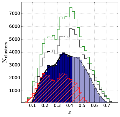
Figure 2: The redshift (left panel) and mass (right panel) distribution of the spectroscopic cluster sample analyzed in this work (blue solid histogram in the selected redshift range $0.1<z<0.42$, cyan histogram at higher redshifts), compared to the redshift distributions of the WHL12 photometric and spectroscopic cluster samples (green and red histogram, respectively) and of the WHL12 sample restricted to the BOSS area (black histogram). The number of selected clusters in each catalog is reported in the label. The black solid line in the left panel shows the smoothed redshift distribution of the random catalog.

3 Clustering measurements

In this Section, we present the methodologies considered in this work to measure the redshift-space wedges of the selected galaxy cluster sample, that will be used to derive constraints on the linear growth rate from RSD.

3.1 Random catalog

To estimate the three-dimensional 2PCF of a sample of extragalactic sources, a geometric selection function is needed. The clustering estimator adopted in this work (see §3.2) requires this function to be provided as a catalog of objects randomly distributed in the same area of the real catalog, and with the same selection along the line of sight. As we will explain in §4, the likelihood we will use to extract cosmological constraints from the analyzed clustering dataset is independent of the catalog completeness, which is the fraction of selected galaxy clusters over the full sample (see Marulli et al., 2018, for a similar analysis). Thus, our final results depend only on the geometric selection that enters the clustering estimator.

We construct the random catalog following the same methodology used in galaxy clustering analyses, in particular, the one used to measure the 2PCF of BOSS galaxies. In the assumption that the angular and redshift distributions of the selected galaxy clusters are independent, we assign angular coordinates, i.e. R.A., decl., and redshifts in two separate steps. The R.A.-decl. coordinates are extracted with MANGLE (Swanson et al., 2008), using publicly available survey footprints. The redshifts are then sampled from the true redshift distribution of the catalog, smoothed with a Gaussian kernel of $\sigma_{z}=0.02$ in order not to introduce spurious clustering along the line of sight. As we verified, the impact of this assumption is negligible. Due to the different density and redshift distributions in the north, north E2, north E3 and south fields, the extraction of random coordinates and redshifts is performed in each field separately. The final random catalog, which is obtained by adding the random catalogs in the four fields, is constructed to be $50$ times larger than the selected cluster catalog in order to minimize the impact of the shot noise. The redshift distribution of the random objects normalized to the number of the spectroscopic cluster sample is shown in Fig. 2.

3.1.1 Weights

We take into account the systematic uncertainties in the angular selection function due to the position-dependent completeness of the cluster sample. To do this, we cross correlate the angular cluster counts with the maps of observational systematics provided by Leistedt & Peiris (2014). We find that the cluster counts are anticorrelated with stellar densities, and less strongly, with the $r$-band extinction. We correct for this effect by weighting the objects in the random sample accordingly.

Moreover, we weight the clusters in the catalog to account for the spectroscopic target selection, following the same weighting scheme adopted by Reid et al. (2016) and Ross et al. (2017):

$$w=w_{\rm see}w_{\rm star}(w_{\rm cp}+w_{\rm noz}-1)\;,$$ (2)

which considers the impact of seeing ($w_{\rm see}$), star contamination ($w_{\rm star}$) and presence of a close target ($w_{\rm cp}$), as well as spectroscopic measurement failures ($w_{\rm noz}$).

3.2 Clustering wedges

The cosmological analysis performed in this work is based on the redshift-space clustering wedges of the 2PCF of the spectroscopic cluster catalog presented in §2.2. The clustering wedges have been introduced by Kazin et al. (2010) as a convenient projection statistic, similar to the clustering multipoles, to compress the anisotropic 2PCF signal. The main advantage of this approach is to reduce the dimension of the dataset to be analyzed, and the associated covariance matrix.

To measure the three-dimensional 2PCF, we first convert the observed coordinates of the galaxy clusters (R.A., decl., redshift) into comoving Cartesian coordinates, assuming Planck18 cosmology.

The comoving distances, $d_{\rm c}$, are related to the cosmological redshifts, $z$, as follows:

$$d_{\rm c}(z)=c\int_{0}^{z}\frac{\mbox{d}z^{\prime}}{H(z^{\prime})}\;,$$ (3)

where $c$ is the speed of light, and $H$ is the Hubble parameter, which in a flat $\Lambda$CDM model reads as

$$H(z)=H_{0}\left[\Omega_{\rm M}(1+z)^{3}+(1-\Omega_{\rm M})\right]^{1/2}\;.$$ (4)

Neglecting redshift uncertainties and second-order corrections, the observed redshift, $z_{\rm obs}$, is related to the cosmological redshift, $z$, as follows:

$$z_{\rm obs}=z+\frac{v_{\parallel}}{c}(1+z)\;,$$ (5)

where $v_{\parallel}$ is the peculiar velocity along the line of sight. In this analysis, the impact of cluster redshift uncertainties on the 2PCF is minor, especially on large scales, as we consider only the spectroscopic cluster sample. Assuming that the cluster spectroscopic redshift uncertainties follow a Gaussian distribution (e.g. Sereno et al., 2015), their effects on the 2PCF are degenerate with those of small-scale peculiar random motions, and do not require any additional parameters to be modeled (see §4).

Since the peculiar velocities of the analyzed cluster sample are unknown, we estimate the comoving distances by substituting $z$ with $z_{\rm obs}$ in Eq. 3, thus introducing the so-called RSD. Hereafter, the redshift-space spatial coordinates are indicated with s.

The anisotropic 2PCF in redshift-space is computed with the Landy & Szalay (1993) estimator:

$$\hat{\xi}(s,\mu)\,=\,\frac{N_{RR}}{N_{CC}}\frac{CC(s,\mu)}{RR(s,\mu)}-2\frac{N_{RR}}{N_{CR}}\frac{CR(s,\mu)}{RR(s,\mu)}+1\,,$$ (6)

where $\mu$ is the cosine of the angle between the line of sight and the comoving separation $s$, $CC(s,\mu)$, $RR(s,\mu),$ and $CR(s,\mu)$ are the numbers of cluster-cluster, random-random, and cluster-random pairs in bins of $s$ and $\mu$, i.e. in $s\pm\Delta s$ and $\mu\pm\Delta\mu$, $N_{C}$ and $N_{R}$ are the total numbers of clusters and random objects, and $N_{CC}=N_{C}(N_{C}-1)/2$, $N_{RR}=N_{R}(N_{R}-1)/2$, and $N_{CR}=N_{C}N_{R}$ are the total numbers of cluster-cluster, random-random, and cluster-random pairs, respectively. The Landy & Szalay (1993) estimator of the 2PCF is widely used as it provides the minimum variance when $|\xi|\ll 1$, and it is unbiased in the limit of an infinitely large random sample (Keihänen et al., 2019). We estimate the comoving separation associated with each bin as the average cluster pair separation inside the bin (e.g. Zehavi et al., 2011).

Lastly, to efficiently compress the information contained in the clustering signal, we estimate the so-called wedges of the 2PCF (Kazin et al., 2012), that consist in the integrals of $\xi(s,\mu)$ over wide bins of $\mu$:

$$\xi_{w}(s)\equiv\frac{1}{\Delta\mu}\int_{\mu_{1}}^{\mu_{2}}\mathrm{d}\mu\,\xi(s,\mu)\,,$$ (7)

where $\Delta\mu=\mu_{2}-\mu_{1}$ is the wedge width. Here, we set $\Delta\mu=0.5$, which leads to two clustering wedges, that is the transverse wedge, $\xi_{\perp}(s)\equiv\xi_{1/2}(\mu_{min}=0,s)$, and the radial wedge, $\xi_{\parallel}(s)\equiv\xi_{1/2}(\mu_{min}=0.5,s)$, computed in the ranges of $0\leq\mu<0.5$ and $0.5\leq\mu\leq 1$, respectively.

4 Modeling

4.1 Redshift-space distortions

We model the redshift-space transverse and radial wedges of the 2PCF of our cluster catalog with an extended version of the Taruya et al. (2010) model, which includes the nonlinear biasing model by McDonald & Roy (2009). Following Beutler et al. (2014), we will refer to this as the extended Taruya, Nishimichi $\&$ Saito (eTNS) model.

The redshift-space power spectrum of galaxy clusters in the eTNS model is approximated as follows:

$$P^{s}(k,\mu)=D(k,\mu,f,\sigma_{v})\biggl{[}P_{\mathrm{c},\delta\delta}(k)+2f\mu^{2}P_{\mathrm{c},\delta\theta}(k)+\\ f^{2}\mu^{4}P_{\theta\theta}(k)+b_{1}^{3}C_{A}(k,\mu,f,b_{1})+b_{1}^{4}C_{B}(k,\mu,f,b_{1})\biggr{]}\,,$$ (8)

where $f$ is the linear growth rate, $b_{1}$ is the linear bias, $\theta(\mathbf{k})\equiv[-i\mathbf{k}\cdot\mathbf{v}(\mathbf{k})]/[af(a)H(a)]$ is the velocity divergence, $P_{\mathrm{c},\delta\delta}(k)$ is the real-space density cluster power spectrum, $P_{\mathrm{c},\delta\theta}(k)$ and $P_{\theta\theta}(k)$ are the real-space density-velocity divergence cross-spectrum and the real-space velocity divergence auto-spectrum of clusters, respectively, assuming no velocity bias, i.e. $P_{\mathrm{c},\theta\theta}(k)=P_{\theta\theta}(k)$, $D(k,f,\mu,\sigma_{v})$ is a damping factor used to model the random peculiar motions at small scales, and $C_{A}$ and $C_{B}$ are two additional terms to correct for systematics at small scales. The cluster power spectra are computed with the nonlinear biasing model by McDonald & Roy (2009) as follows:

$$P_{\mathrm{c},\delta\delta}(k)=b_{1}^{2}P_{\delta\delta}(k)+2b_{2}b_{1}P_{b2,\delta}(k)+2b_{s^{2}}b_{1}P_{bs2,\delta}(k)\\ +2b_{3\mathrm{nl}}b_{1}\sigma_{3}^{2}(k)P_{\mathrm{m}}^{\mathrm{lin}}(k)+b_{2}^{2}P_{b22}(k)\\ +2b_{2}b_{s^{2}}P_{b2s2}(k)+b_{s^{2}}^{2}P_{bs22}(k)+N\,,$$ (9)

$$P_{\mathrm{c},\delta\theta}(k)=b_{1}P_{\delta\theta}(k)+b_{2}P_{b2,\theta}(k)+b_{s^{2}}P_{bs2,\theta}(k)\\ +b_{3\mathrm{nl}}\sigma_{3}^{2}(k)P_{\mathrm{m}}^{\mathrm{lin}}(k)\,,$$ (10)

where $P_{\mathrm{m}}^{\mathrm{lin}}(k)$ is the linear power spectrum. The adopted biasing model has the following four parameters, besides the linear bias term, $b_{1}$: the second-order local and nonlocal bias parameters, $b_{2}$ and $b_{s^{2}}$, the third-order nonlocal bias parameter, $b_{3\mathrm{nl}}$, and the constant stochasticity term, $N$. The latter parameter affects only the smallest comoving separations, which are not considered in our analysis. As we verified, its impact on the cosmological outcomes of this work is in fact negligible. In the local Lagrangian framework the nonlocal bias terms can be written as a function of $b_{1}$ as follows (Chan et al., 2012; Saito et al., 2014):

$$b_{s^{2}}=-\frac{4}{7}(b_{1}-1)\,,$$ (11)

$$b_{3\mathrm{nl}}=\frac{32}{315}(b_{1}-1)\,.$$ (12)

The $P_{\delta\delta}(k)$, $P_{\delta\theta}(k)$ and $P_{\theta\theta}(k)$ terms are estimated in the standard perturbation theory (SPT), which consists of expanding the statistics as a sum of infinite terms, corresponding to the $n$-loop corrections (see e.g. Gil-Marín et al., 2012). Considering corrections up to the first loop order, the matter power spectrum can be modeled as follows:

$$P^{\mathrm{SPT}}(k)=P_{\mathrm{m}}^{\mathrm{lin}}(k)+2P_{13}(k)+P_{22}(k)\,,$$ (13)

where the one-loop correction terms are computed with the CPT Library (Taruya & Hiramatsu, 2008; Zhao et al., 2021). To test the model accuracy, we compared the outcomes of our reference analysis with the ones obtained by adopting the Bel et al. (2019) universal fitting functions for $P_{\delta\theta}(k)$ and $P_{\theta\theta}(k)$, finding negligible differences (see also Pezzotta et al., 2017; de la Torre et al., 2017). The other power spectrum terms in Eqs. (9) and  (10), that is $P_{b2,\delta}(k)$, $P_{bs2,\delta}(k)$, $P_{b22}(k)$, $P_{b2s2}(k)$, $P_{bs22}(k)$, $P_{b2,\theta}(k)$ and $P_{bs2,\theta}(k)$, are computed as a function of $P_{\mathrm{m}}^{\mathrm{lin}}(k)$, as prescribed in e.g. Beutler et al. (2014) and Gil-Marín et al. (2014).

The damping term is assumed to be Lorentzian in Fourier space (see e.g. de la Torre et al., 2017):

$$D(k,f,\mu,\sigma_{v})=\frac{1}{1+k^{2}f^{2}\mu^{2}\sigma_{v}^{2}}\,,$$ (14)

where $\sigma_{v}$ is a nuisance parameter to marginalize over (Davis & Peebles, 1983; Fisher et al., 1994; Zurek et al., 1994).

Finally, we compute the correction terms $C_{A}$ and $C_{B}$ in Eq. (8) in SPT as follows (Taruya et al., 2010; de la Torre & Guzzo, 2012):

$$\begin{split}C_{A}(k,\mu,f,b_{1})&=(k\mu f)\int\frac{\mathrm{d}^{3}\boldsymbol{p}}{(2\pi)^{3}}\frac{p_{z}}{p^{2}}\\ &\times\left[B_{\sigma}(\boldsymbol{p},\boldsymbol{k}-\boldsymbol{p},-\boldsymbol{k})-B_{\sigma}(\boldsymbol{p},\boldsymbol{k},-\boldsymbol{k}-\boldsymbol{p})\right]\,,\end{split}$$ (15)

$$C_{B}(k,\mu,f,b_{1}) =(k\mu f)^{2}\int\frac{\mathrm{d}^{3}\boldsymbol{p}}{(2\pi)^{3}}F(\boldsymbol{p})F(\boldsymbol{k}-\boldsymbol{p})\,,$$ (16)

$$F(\boldsymbol{p}) =\frac{p_{z}}{p^{2}}\left[P_{\delta\theta}(p)+f\frac{p_{z}^{2}}{p^{2}}P_{\theta\theta}(p)\right]\,,$$ (17)

where $B_{\sigma}$ is the cross bispectrum. The $C_{A}$ and $C_{B}$ terms are proportional to $b_{1}^{3}$ and $b_{1}^{4}$, respectively, and can be expressed as a power series expansion of $b_{1}$, $f$ and $\mu$ (see e.g. García-Farieta et al., 2019, 2020, for more details).

We note that the eTNS model given by Eq. (8) reduces to the Taruya et al. (2010) model if all the nonlinear bias terms are neglected, to the Scoccimarro (2004) model if also the $C_{A}$ and $C_{B}$ terms are neglected, and to the so-called dispersion model if both $P_{\delta\theta}(k)$ and $P_{\theta\theta}(k)$ are approximated as $P_{\delta\delta}(k)$, which is valid in the linear regime (Kaiser, 1987; Peacock & Dodds, 1996).

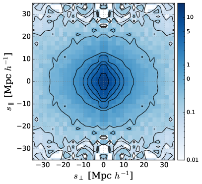
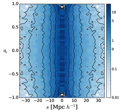
Figure 3: The redshift-space 2PCF of the spectroscopic cluster catalog. Left panel: 2PCF in Cartesian coordinates, which is as a function of perpendicular and parallel separations to the line of sight. Right panel: 2PCF in polar coordinates, that is as a function of distance modulus and cosine of the angle between the line of sight.

The power spectrum multipoles can be estimated from Eq. (8), as follows:

$$P_{l}(k)=\frac{2l+1}{2\alpha_{\perp}^{2}\alpha_{\parallel}}\int_{-1}^{1}\mbox{d}\mu\,P^{s}(k^{\prime},\mu^{\prime})L_{l}(\mu)\,,$$ (18)

where the Alcock & Paczynski (1979) (AP) geometric distortions, caused by a possibly incorrect assumption of the background cosmology used to convert cluster redshifts into comoving distances in Eq. (3), are modeled by rescaling the wave numbers as follows (Beutler et al., 2014):

$$k^{\prime}=\frac{k}{\alpha_{\perp}}\left[1+\mu^{2}\left(\frac{\alpha^{2}_{\perp}}{\alpha^{2}_{\parallel}}-1\right)\right]^{1/2}\,,$$ (19)

$$\mu^{\prime}=\mu\frac{\alpha_{\perp}}{\alpha_{\parallel}}\left[1+\mu^{2}\left(\frac{\alpha^{2}_{\perp}}{\alpha^{2}_{\parallel}}-1\right)\right]^{-1/2}\,,$$ (20)

with

$$\alpha_{\parallel}=\frac{H^{\rm fid}(z)r_{s}^{\rm fid}(z_{d})}{H(z)r_{s}(z_{d})}\,,$$ (21)

$$\alpha_{\perp}=\frac{D_{A}(z)r_{s}^{\rm fid}(z_{d})}{D_{A}^{\rm fid}(z)r_{s}(z_{d})}\,,$$ (22)

where $H^{\rm fid}(z)$ and $D_{A}^{\rm fid}(z)$ are the fiducial values for the Hubble constant and angular diameter distance, respectively, and $r_{s}^{\rm fid}(z_{d})$ is the fiducial sound horizon at the drag redshift assumed in the power spectrum template.

The corresponding 2PCF multipoles in configuration space read as

$$\xi_{l}(s)=i^{l}\int_{-\infty}^{\infty}\frac{\mbox{d}k}{2\pi^{2}}k^{2}P_{l}(k)j_{l}(ks)\,,$$ (23)

where $L_{l}(\mu)$ are the Legendre polynomials and $j_{l}$ are the spherical Bessel functions of order $l$.

Lastly, we assess the redshift-space wedges from the multipole moments through the following relation:

$$\xi_{w}(r)=\sum_{l}\xi_{l}(s)\bar{L}_{l}\,,$$ (24)

where $\bar{L}_{l}$ is the average value of the Legendre polynomials over the interval $[\mu_{1},\mu_{2}]$. In particular, neglecting minor contributions from multipoles with $l>2$ and considering the wedge width $\Delta\mu=0.5$, Eq. (24) can be written as follows (Kazin et al., 2012):

$$\left(\begin{array}[]{l}{\xi_{\|}}\\ {\xi_{\perp}}\end{array}\right)=\left(\begin{array}[]{cc}{1}&{\frac{3}{8}}\\ {1}&{-\frac{3}{8}}\end{array}\right)\left(\begin{array}[]{c}{\xi_{0}}\\ {\xi_{2}}\end{array}\right)\,.$$ (25)

A full validation of the implemented likelihood algorithms on simulated galaxy and cluster catalogs will be presented in a forthcoming paper (García-Farieta et al., in prep.).

As a common practice, and to directly compare to previous similar analyses performed on galaxy samples, we parameterize the model as a function of $\sigma_{v}$ and the three parameter products $\left[f\sigma_{8},\,b_{1}\sigma_{8},\,b_{2}\sigma_{8}\right]$ (but see Sánchez, 2020), fixing the other parameters to Planck18 cosmology.

In this work we focus on scales smaller than the BAO ones, which does not allow us to put strong enough constraints on the geometric distortions that are degenerate with RSD (e.g. Taruya et al., 2011). Nevertheless, to marginalize over the AP distortion parameters, we allow them to vary, considering Gaussian priors with standard deviation of $0.01$ (see e.g. de la Torre et al., 2017, for a similar approach).

The posterior distribution constraints on these parameters are assessed through a Markov Chain Monte Carlo (MCMC) statistical analysis, assuming a standard Gaussian likelihood:

$$-2\ln\mathcal{L}=\sum_{i,j=1}^{N}\left[\xi_{k}^{D}(s_{i})-\xi_{k}^{M}(s_{i})\right]C_{k}^{-1}(s_{i},s_{j})\left[\xi_{k}^{D}(s_{j})-\xi_{k}^{M}(s_{j})\right]\,,$$ (26)

where $N$ is the number of bins at which the wedges are computed, and the superscripts $D$ and $M$ refer to data and model, respectively.

The covariance matrix, $C_{k}$, which measures the variance and correlation between 2PCF wedge bins, is defined as follows:

$$C_{w}\left(s_{i},s_{j}\right)=\frac{1}{N_{R}-1}\sum_{n=1}^{N_{R}}\left[\xi_{w}^{n}\left(s_{i}\right)-\overline{\xi}_{w}\left(s_{i}\right)\right]\left[\xi_{w}^{n}\left(s_{j}\right)-\overline{\xi}_{w}\left(s_{j}\right)\right]\,.$$ (27)

The indices $i$ and $j$ run over the 2PCF wedge bins, while $w=0,0.5$ refers to each clustering wedge. In both cases, $\bar{\xi}_{w}=1/N_{R}\sum_{n=1}^{N_{R}}\xi_{w}^{n}$ is the average wedge of the 2PCF, and $N_{R}=100$ is the number of realizations obtained by resampling the catalogs with the bootstrap method. We correct the inverse covariance matrix estimator to account for the finite number of realizations as in Hartlap et al. (2007), while the parameter uncertainties are corrected to take into account the uncertainties in the covariance estimate as in Percival et al. (2014).

4.2 Exploiting cluster masses

Similarly to RSD analyses of galaxy clustering, we adopt large flat priors on $f\sigma_{8}$, $b_{2}\sigma_{8}$ and $\sigma_{v}$, specifically $f\sigma_{8}=\left[0,1\right]$, $b_{2}\sigma_{8}=\left[-10,10\right]$ and $\sigma_{v}=\left[0,100\right]\mbox{Mpc}\,h^{-1}$, respectively. While $\sigma_{8}$ could be constrained directly from the cluster mass function, this would have required an accurate knowledge of the cluster selection function to avoid systematic uncertainties. To provide conservative linear growth constraints, we prefer to focus the current analysis on cluster clustering, setting all the cosmological parameters, including $\sigma_{8}$, to Planck18 values. The constraint on the linear growth rate we will derive in this paper has to be considered in this respect, though to compare to previous analyses we will express our results in terms of $f\sigma_{8}$.

Differently from galaxy clustering analyses, we can set a strong prior on $b_{1}\sigma_{8}$ thanks to the knowledge of galaxy cluster masses inferred from weak-lensing scaling relations. In particular, the $b_{1}\sigma_{8}$ prior is centered on the effective linear bias of the cluster sample, which is estimated as in Marulli et al. (2018):

$$b_{\rm eff}^{2}=<b(\tilde{M}_{i},z_{i})b(\tilde{M}_{j},z_{j})>\;,$$ (28)

where the linear bias of each cluster, $b$, is computed with the Tinker et al. (2010) model, while $\tilde{M_{i}}$ and $\tilde{M_{j}}$ are the masses of the two clusters of each pair, at redshifts $z_{i}$ and $z_{j}$, respectively, estimated from the weak-lensing cluster mass scaling relation given by Eq. (1). This represents the key difference with respect to analogous RSD analyses of galaxy samples, as in those cases the masses of the dark matter haloes hosting the galaxies are unknown and no priors can be reliably assumed on the bias of the catalog. We will discuss the impact of this assumption in §5.

Drawing a set of mass samples from the scaling relation, we computed the average bias and variance of our cluster catalog, which correspond to $b_{1}\sigma_{8}=1.722\pm 0.002$. We consider a Gaussian prior on $b_{1}\sigma_{8}$ centered on the latter value. To provide conservative constraints, we adopt a prior width $5$ times larger than the estimated standard deviation, i.e., $0.01$, to include possible systematic uncertainties in the adopted bias model and scaling relation.

5 Results

5.1 Constraints on the growth rate

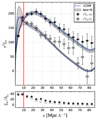
Figure 4: Upper panel: The redshift-space transverse (solid circles) and radial (open squares) wedges of the spectroscopic cluster catalog compared to the best-fit eTNS model, which is the median of the MCMC posterior distribution (black solid line). The shaded areas show the $68\%$ uncertainty on the posterior median. The horizontal error bars are the standard deviation around the mean pair separation in each bin. The vertical error bars show the diagonal values of the bootstrap covariance matrix. The vertical red line indicates the minimum scale used in the fitting analysis. The minor mismatch in the radial wedge at $40<s\left[\mbox{Mpc}\,h^{-1}\right]<60$ is not statistically significant considering the covariance in the measurements ($\tilde{\chi}^{2}=0.71$). Lower panel: The signal-to-noise ratio, that is the transverse (solid circles) and radial (open squares) wedge values divided by the corresponding standard deviations.

Figure 5: The bootstrap correlation matrix $\left(C_{i,j}/\sqrt{C_{i,j}C_{j,i}}\right)$ of the redshift-space transverse and radial wedges of the spectroscopic cluster catalog.

As described in §3, the clustering wedges are computed by integrating the redshift-space 2PCF, $\xi(s,\mu)$, over two bins of $\mu$. In Fig. 3 we present the redshift-space 2PCF of the selected cluster sample in two coordinate systems, i.e., as a function of perpendicular ($s_{\perp}$) and parallel ($s_{\parallel}$) separations to the line of sight (Cartesian coordinates), and as a function of distance modulus ($s$) and cosine of the angle ($\mu$) between the line of sight (polar coordinates). In real space the contour lines of the former statistics would be circular, while the ones of the latter statistics would be straight. RSD introduce anisotropies in the derived map that warp these contour lines, an effect that depends directly on the value of the linear growth rate of cosmic structures.

The shape of the Cartesian 2PCF of the selected clusters shown in the left panel of Fig. 3 appears similar to the one of galaxies, as expected (e.g. Alam et al., 2017; Marulli et al., 2017). In fact, as described in §2.2, the 2PCF of galaxy clusters we measure in this work coincides with the 2PCF of BCGs, by construction. Nevertheless, the cosmological analysis of this dataset provides a clear advantage as, differently from galaxy clustering studies, we can infer in this case the linear bias of the sample from the richness-mass scaling relation of the galaxy clusters hosting the selected BCGs, as explained in §4.2.

The Fingers-of-God distortions at small scales due to incoherent peculiar motions are not completely negligible, though much less strong relative to the case of the 2PCF of lower biased tracers (see the discussion in Marulli et al., 2017). The polar 2PCF shown in the right panel of Fig. 3 is the statistics we integrate along the $\mu$ direction to compute the wedges.

Figure 4 shows the redshift-space transverse and radial wedges of the cluster 2PCF, defined by Eq. (7). The horizontal and vertical error bars are the standard deviation around the mean pair separation in each bin, and the diagonal values of the bootstrap covariance matrix, respectively. In real space, the radial and transverse wedges would be statistically equal, for isotropy. On the other hand, redshift-space anisotropies make these two statistics significantly different, as shown in Fig. 4.

Figure 6: Comparison between the diagonal values of different covariance matrix estimates of the redshift-space transverse (solid lines) and radial (dashed lines) wedges of the spectroscopic cluster catalog. Blue and green lines refer to the bootstrap and jackknife covariance matrix, respectively. Black lines refer to the theoretical covariance matrix by Grieb et al. (2016), comprising both the shot noise (SN) and cosmic variance (CV) contributions, while red lines include only the contribution of cosmic variance.

The correlation matrix, which is $C_{i,j}/\sqrt{C_{i,j}C_{j,i}}$, of the redshift-space transverse and radial wedges is shown in Fig. 5. The algorithms to estimate the covariance matrix have been highly validated in previous works on both simulations and real cluster catalogs (e.g. Veropalumbo et al., 2014, 2016; Marulli et al., 2017; García-Farieta et al., 2020). To further check the results of the current analysis, we compare the bootstrap error estimates with the ones obtained with either the jackknife method or the analytic Gaussian model provided by Grieb et al. (2016) (for the theoretical modeling of non-Gaussian contributions to the covariance, which are neglected in the current analysis, see Sugiyama et al., 2020). The diagonal values of the bootstrap, jackknife, and analytic matrices are compared in Fig. 6. The estimated bootstrap clustering uncertainties are statistically consistent with the analytic ones at scales larger than about $20$ $h^{-1}\,\mbox{Mpc}$ , while the jackknife uncertainties appear slightly larger.

The bootstrap method allows us to draw a greater number of realizations relative to the jackknife method, providing a smoother covariance matrix, whose inverse is less affected by numerical noise. Moreover, it does not depend on free parameters, differently from the analytic covariance matrix, which depends on the sample bias and on the effective area of the survey, whose values are inferred within uncertainties. For the above reasons, in this work we rely on the bootstrap covariance uncertainties.

Following the method described in §4, we perform a joint statistical analysis of the redshift-space radial and transverse wedges of the selected spectroscopic cluster catalog, in the standard $\Lambda$CDM framework. The best-fit eTNS model obtained from the median of the MCMC posterior distribution is reported in Fig. 4, together with its $68\%$ uncertainty region. The fit is performed in the comoving scale range $10<s\left[\mbox{Mpc}\,h^{-1}\right]<80$. The model appears statistically consistent with the measurements in the scale range considered. We note only a minor mismatch in the radial wedge at $40<s\left[\mbox{Mpc}\,h^{-1}\right]<60$, though it is not statistically significant considering the covariance in the measurements. The reduced $\chi^{2}$ at the best-fit eTNS model is $\tilde{\chi}^{2}=-2\ln\mathcal{L}/\mbox{d.o.f.}=0.71$ (where d.o.f. are the degrees of freedom of the data sample).

The marginalized posterior distributions on $f\sigma_{8}$, $b_{1}\sigma_{8}$, $b_{2}\sigma_{8}$ and $\sigma_{v}$ are reported in Fig. 7, together with the $68\%$ and $95\%$ posterior confidence regions. We assess the best-fit values and marginalized constraints from the median and percentile values of the posterior distribution. We note in particular that the $f\sigma_{8}$ posterior is consistent with a Gaussian distribution. We get $f\sigma_{8}=0.44\pm 0.05$, at the mean pair redshift $z=0.275$. The relative statistical uncertainty is about $10\%$, which is a remarkable result considering the sparsity of the spectroscopic cluster sample considered. This is caused by the narrow Gaussian prior on the effective bias of the sample, assessed through the cluster mass-richness scaling relation, as described in §4. In fact, the posterior distribution we get on $b_{1}\sigma_{8}$ is statistically indistinguishable from the assumed Gaussian prior distribution.

We tested the impact of this assumption by running the statistical analysis assuming prior standard deviations of $0.002$, $0.05$ and $0.1$. In particular, the latter prior width accounts for possible bias model uncertainties of about $5\%$. We obtained $f\sigma_{8}=0.44\pm 0.05$, $f\sigma_{8}=0.42\pm 0.06$ and $f\sigma_{8}=0.41\pm 0.06$, respectively, which are all statistically consistent, considering current measurement uncertainties. Assuming instead a flat prior distribution on $b_{1}\sigma_{8}$ in $\left[0.1,5\right]$, we get $f\sigma_{8}=0.40\pm 0.07$, which is still statistically consistent with our fiducial result, though with a larger relative error of about $18\%$.

All the results obtained for the different prior assumptions considered are statistically consistent, showing that the accuracy in the mass estimates and in the linear bias model is high enough for the current analysis. Improving the mass and bias modeling will become crucial instead for cluster clustering analyses of next-generation surveys.

The reference value of the quadratic bias factor, $b_{2}\sigma_{8}$, reported in Fig. 7 is computed with the polynomial relation provided by Lazeyras et al. (2016):

$$b_{2}(b_{1})=0.412-2.143\,b_{1}+0.929\,b_{1}^{2}+0.008\,b_{1}^{3}\;,$$ (29)

while the reference value of $\sigma_{v}$ is estimated in linear theory as follows (Taruya et al., 2010):

$$\sigma_{\mathrm{v},\mathrm{lin}}^{2}=\frac{1}{3}\int\frac{\mathrm{d}^{3}\boldsymbol{q}}{(2\pi)^{3}}\frac{P_{\mathrm{m}}^{\mathrm{lin}}(q,z)}{q^{2}}\;.$$ (30)

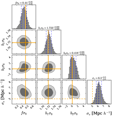
Figure 7: $68\%$ and $95\%$ posterior confidence regions for the four eTNS parameters $f\sigma_{8}$, $b_{1}\sigma_{8}$, $b_{2}\sigma_{8}$, $\sigma_{v}$, obtained from the MCMC modeling of the redshift-space radial and transverse wedges of galaxy clusters in the scale range $10<s\left[\mbox{Mpc}\,h^{-1}\right]<80$. The vertical dashed blue lines show the first quantiles of the 1D marginalized distributions. The solid orange lines show the Planck18 $f\sigma_{8}$, $b_{1}\sigma_{8}$ and $b_{2}\sigma_{8}$ predictions, with $b_{1}$ being estimated by Eq. (28) with Tinker et al. (2010) model, and $b_{2}$ from Eq. (29). The dashed orange lines show the linear-order estimate of the one-dimensional velocity dispersion given by Eq. (30).

To test the robustness of our results, we repeated the analysis fitting the wedges in narrower scale ranges, considering either jackknife or analytic clustering uncertainties instead of boostrap, and modeling small-scale random motions with a Gaussian damping term instead of a Lorentzian one (Marulli et al., 2012; Sridhar et al., 2017; García-Farieta et al., 2020). Overall we found consistent results, within the $68\%$ confidence region.

As discussed in §4.1, we considered tight Gaussian priors on the AP distortion parameters with standard deviation of $0.01$. To investigate the impact of this assumption, we run our analysis also for standard deviation values of $0$, $0.05$ and $0.1$, obtaining $f\sigma_{8}=0.44\pm 0.05$, $f\sigma_{8}=0.4\pm 0.1$ and $f\sigma_{8}=0.3\pm 0.2$, respectively. As expected, the impact of this prior is significant. Since the current analysis focuses on scales below the BAO peak, we cannot break the degeneracy between RSD and geometric distortions. Constraints from a joint RSD+BAO analysis of both the two-point and three-point correlation functions of this cluster sample is presented in Veropalumbo et al. (in prep.).

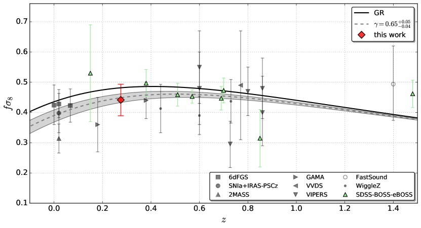
Figure 8: Constraints on $f\sigma_{8}$ from the redshift-space wedges of the galaxy cluster sample considered in this work (red diamond) compared to a compilation of recent measurements exploiting different techniques applied to the following surveys: 6dFGS (Beutler et al., 2012; Huterer et al., 2017; Adams & Blake, 2017); ‘First Amendment’ set of SNe peculiar velocities (Turnbull et al., 2012); 2MASS (Davis et al., 2011); GAMA (Blake et al., 2013); WiggleZ (Blake et al., 2012); VVDS (Guzzo et al., 2008); VIPERS (de la Torre et al., 2013, 2017; Pezzotta et al., 2017; Hawken et al., 2017; Mohammad et al., 2018); FastSound (Okumura et al., 2016); SDSS+BOSS+eBOSS (Alam et al., 2021). The black solid line shows the standard $\Lambda$CDM + GR Planck18 prediction, while the dashed gray line and shaded area show the model with $\gamma=0.65^{+0.05}_{-0.04}$ (Moresco & Marulli, 2017).

5.2 Comparison to previous data and models

In Fig. 8 we compare the $f\sigma_{8}$ constraint obtained in this work with a large collection of measurements at different redshifts from galaxy, quasar, and cosmic void samples and other tracers. The data shown provide the key observables to test the gravity theory on the largest cosmological scales. Figure 8 summarizes our current understanding of the cosmological evolution of the linear growth rate of cosmic structures. Specifically, the data reported are from 6dF Galaxy Survey (6dFGS) (Beutler et al., 2012; Huterer et al., 2017; Adams & Blake, 2017); ‘First Amendment’ set of SNe peculiar velocities (Turnbull et al., 2012); 2MASS (Davis et al., 2011); Galaxy And Mass Assembly (GAMA) (Blake et al., 2013); WiggleZ (Blake et al., 2012); VIMOS-VLT Deep Survey (VVDS) (Guzzo et al., 2008); VIMOS Public Extragalactic Redshift Survey (VIPERS) (de la Torre et al., 2013, 2017; Pezzotta et al., 2017; Hawken et al., 2017; Mohammad et al., 2018); FastSound (Okumura et al., 2016); SDSS+BOSS+eBOSS (Howlett et al., 2015; Alam et al., 2017; Nadathur et al., 2019, 2020; Gil-Marín et al., 2020; Tamone et al., 2020; Neveux et al., 2020; Alam et al., 2021; Hou et al., 2021; de Mattia et al., 2021; Bautista et al., 2021). The latest, most constraining measurements from SDSS+BOSS+eBOSS are highlighted in green.

The data are compared to the standard $\Lambda$CDM + general relativity (GR) predictions, which is $f\sigma_{8}=\Omega_{M}(z)^{0.545}\sigma_{8}(z)$, where $\sigma_{8}$ and $\Omega_{M}$ are computed assuming the Planck18 cosmological parameters. The $f\sigma_{8}$ constraint obtained in this work appears fully consistent with the other data, with a competitive statistical uncertainty. By comparison, we also plot the model with $\gamma=0.65^{+0.05}_{-0.04}$, which provides a better fit to the $H(z)/H_{0}-f(z)\sigma_{8}(z)$ diagram, as found by Moresco & Marulli (2017).

The exploitation of growth rate measurements at different redshifts to discriminate among alternative dark energy and modified gravity models would require a detailed study which is outside the scope of this work. Nevertheless, to highlight the constraining power of current cluster clustering measurements, we compare in Fig. 9 the $f\sigma_{8}$ constraint obtained in this work with the predictions of three popular alternative models, that is the f($R$) model (e.g. De Felice & Tsujikawa, 2010), the coupled dark energy (cDE) model (Wetterich, 1995; Amendola, 2000) and the Dvali-Gabadaze-Porrati (DGP) model (Dvali et al., 2000).

The linear growth rate in f($R$) and DGP models can be expressed with the so-called $\gamma$-parameterization:

$$f=\Omega_{M}(z)^{\gamma(z)}\,,$$ (31)

where

$$\gamma(z)=\gamma_{0}+\gamma_{1}\frac{z}{1+z}\,.$$ (32)

In particular, we consider the f($R$) model by Hu & Sawicki (2007), setting the two free model parameters to $n=2$ and $\lambda=3$ following Di Porto et al. (2012), which corresponds to $\gamma_{1}=0.43$ and $\gamma_{2}=-0.2$ in the limit of small, still linear, scales (Gannouji et al., 2009). For the DGP model we consider the flat-space case in which $\gamma_{1}=0.633$ and $\gamma_{2}=0.041$ (Maartens & Majerotto, 2006; Fu et al., 2009). Finally, we model the linear growth rate in the cDE model with the so-called $\eta$-parameterization (di Porto & Amendola, 2008):

$$f=\Omega_{M}(z)^{\gamma}(1+\eta)\,,$$ (33)

where $\eta=c\beta_{c}^{2}$ quantifies the coupling strength. In particular, we consider the case with $\gamma=0.56$, $c=2.1$ and $\beta_{c}=0.16$, which implies $\eta=0.056$ (di Porto & Amendola, 2008; Di Porto et al., 2012).

As shown in Fig. 9, the current measurement uncertainties are not low enough to discriminate between these alternative cosmological scenarios at sufficient statistical level. Next-generation experiments will have instead the required accuracy to achieve this key scientific task (e.g. Amendola et al., 2018).

Figure 9: Comparison between the $f\sigma_{8}$ constraint obtained in this work (red diamonds) with the predictions of different gravity models: GR (black solid line), f($R$) (red dotted line), cDE (green dashed line), DGP (blue dash-dotted line).

6 Conclusions

In this work we provided new constraints on the linear growth rate of cosmic structures from the redshift-space 2PCF of a large spectroscopic cluster sample extracted for the BOSS survey. Cluster clustering is a novel cosmological probe that can now be fully exploited thanks to the large cluster samples currently available, providing cosmological constraints complementary to the ones from standard galaxy clustering RSD analyses. The main advantage of this probe relative to galaxy clustering is the possibility to estimate cluster masses. In particular, taking advantage of the information coming from the weak-lensing cluster mass-richness scaling relation, we could set a sharp prior on the effective bias of the sample.

The main results of this work can be summarized as follows:

• We constructed a large spectroscopic catalog of optically selected clusters from the SDSS in the redshift range $0.1<z<0.42$. The selected sample consists of $43743$ clusters, whose angular coordinates and redshifts are defined as the ones of their BCGs. The cluster masses have been estimated from weak-lensing calibrated scaling relations.

• We measured the redshift-space 2PCF, as well as the transverse and radial 2PCF wedges, finding results consistent with theoretical expectations.

• Assuming a $\Lambda$CDM cosmological model with Planck18 parameters, we modeled the 2PCF wedges with the eTNS model. We performed a MCMC Bayesian analysis to sample the posterior distribution of $f\sigma_{8}$, $b_{1}\sigma_{8}$, $b_{2}\sigma_{8}$, $\sigma_{v}$. The cluster masses are used to set a robust prior on $b_{1}\sigma_{8}$.

• We get $f\sigma_{8}=0.44\pm 0.05$ at the mean pair redshift $z=0.275$, which is fully consistent with $\Lambda$CDM + GR predictions, and with a statistical uncertainty that is competitive with the current state-of-the-art constraints from other probes.

Next-generation projects like the extended Roentgen Survey with an Imaging Telescope Array (eROSITA) satellite mission (Merloni et al., 2012), the NASA’s Nancy Grace Roman Space Telescope (Spergel et al., 2015), the ESA Euclid mission (Laureijs et al., 2011; Sartoris et al., 2016; Amendola et al., 2018) and the Vera C. Rubin Observatory LSST (LSST Dark Energy Science Collaboration, 2012) will provide huge well-characterized cluster samples up to high redshifts. While the main cosmological probe to be exploited is the redshift evolution of cluster number counts, this work also demonstrates that the clustering of galaxy clusters provides key cosmological information. In particular, robust constraints on the cosmic growth rate can be extracted from the redshift-space anisotropies, thus testing the gravity theory on cosmological scales. Moreover, BAO in cluster clustering provide a powerful independent cosmological probe (Veropalumbo et al., 2014, 2016). In Moresco et al. (2021) and Veropalumbo et al. (in prep.) we exploit the same spectroscopic cluster catalog analyzed in this work, measuring the two-point and three-point correlation functions up to the BAO scales, and providing new constraints on the geometry of the universe and on the nonlinear bias of the sample.

References

- Adams & Blake (2017) Adams, C., & Blake, C. 2017, Mon. Not. R. Astron. Soc., 471, 839, doi: 10.1093/mnras/stx1529
- Aihara et al. (2011) Aihara, H., Allende Prieto, C., An, D., et al. 2011, Astrophys. J. Suppl., 193, 29, doi: 10.1088/0067-0049/193/2/29
- Alam et al. (2015) Alam, S., Albareti, F. D., Allende Prieto, C., et al. 2015, Astrophys. J. Suppl., 219, 12, doi: 10.1088/0067-0049/219/1/12
- Alam et al. (2017) Alam, S., Ata, M., Bailey, S., et al. 2017, Mon. Not. R. Astron. Soc., 470, 2617, doi: 10.1093/mnras/stx721
- Alam et al. (2021) Alam, S., Aubert, M., Avila, S., et al. 2021, Phys. Rev. D, 103, 083533, doi: 10.1103/PhysRevD.103.083533
- Alcock & Paczynski (1979) Alcock, C., & Paczynski, B. 1979, Nature, 281, 358, doi: 10.1038/281358a0
- Amendola (2000) Amendola, L. 2000, Phys. Rev. D, 62, 043511, doi: 10.1103/PhysRevD.62.043511
- Amendola et al. (2018) Amendola, L., Appleby, S., Avgoustidis, A., et al. 2018, Living Reviews in Relativity, 21, 2, doi: 10.1007/s41114-017-0010-3
- Angulo et al. (2005) Angulo, R. E., Baugh, C. M., Frenk, C. S., et al. 2005, Mon. Not. R. Astron. Soc., 362, L25, doi: 10.1111/j.1745-3933.2005.00067.x
- Aubert et al. (2020) Aubert, M., Cousinou, M.-C., Escoffier, S., et al. 2020, arXiv e-prints, arXiv:2007.09013. https://arxiv.org/abs/2007.09013
- Balaguera-Antolínez et al. (2011) Balaguera-Antolínez, A., Sánchez, A. G., Böhringer, H., et al. 2011, Mon. Not. R. Astron. Soc., 413, 386, doi: 10.1111/j.1365-2966.2010.18143.x
- Bautista et al. (2021) Bautista, J. E., Paviot, R., Vargas Magaña, M., et al. 2021, Mon. Not. R. Astron. Soc., 500, 736, doi: 10.1093/mnras/staa2800
- Bel et al. (2019) Bel, J., Pezzotta, A., Carbone, C., Sefusatti, E., & Guzzo, L. 2019, Astron. Astrophys., 622, A109, doi: 10.1051/0004-6361/201834513
- Berlind et al. (2006) Berlind, A. A., Frieman, J., Weinberg, D. H., et al. 2006, Astrophys. J. Suppl., 167, 1, doi: 10.1086/508170
- Beutler et al. (2012) Beutler, F., Blake, C., Colless, M., et al. 2012, Mon. Not. R. Astron. Soc., 423, 3430, doi: 10.1111/j.1365-2966.2012.21136.x
- Beutler et al. (2014) Beutler, F., Saito, S., Seo, H.-J., et al. 2014, Mon. Not. R. Astron. Soc., 443, 1065, doi: 10.1093/mnras/stu1051
- Beutler et al. (2017) Beutler, F., Seo, H.-J., Saito, S., et al. 2017, Mon. Not. R. Astron. Soc., 466, 2242, doi: 10.1093/mnras/stw3298
- Blake et al. (2012) Blake, C., Brough, S., Colless, M., et al. 2012, Mon. Not. R. Astron. Soc., 425, 405, doi: 10.1111/j.1365-2966.2012.21473.x
- Blake et al. (2013) Blake, C., Baldry, I. K., Bland-Hawthorn, J., et al. 2013, Mon. Not. R. Astron. Soc., 436, 3089, doi: 10.1093/mnras/stt1791
- Blanton et al. (2003) Blanton, M. R., Hogg, D. W., Bahcall, N. A., et al. 2003, Astrophys. J., 592, 819, doi: 10.1086/375776
- Chan et al. (2012) Chan, K. C., Scoccimarro, R., & Sheth, R. K. 2012, Phys. Rev. D, 85, 083509, doi: 10.1103/PhysRevD.85.083509
- Chuang & Wang (2013) Chuang, C.-H., & Wang, Y. 2013, Mon. Not. R. Astron. Soc., 435, 255, doi: 10.1093/mnras/stt1290
- Chuang et al. (2013) Chuang, C.-H., Prada, F., Cuesta, A. J., et al. 2013, Mon. Not. R. Astron. Soc., 433, 3559, doi: 10.1093/mnras/stt988
- Chuang et al. (2016) Chuang, C.-H., Prada, F., Pellejero-Ibanez, M., et al. 2016, Mon. Not. R. Astron. Soc., 461, 3781, doi: 10.1093/mnras/stw1535
- Costanzi et al. (2019) Costanzi, M., Rozo, E., Simet, M., et al. 2019, Mon. Not. R. Astron. Soc., 488, 4779, doi: 10.1093/mnras/stz1949
- Covone et al. (2014) Covone, G., Sereno, M., Kilbinger, M., & Cardone, V. F. 2014, Astrophys. J. Lett., 784, L25, doi: 10.1088/2041-8205/784/2/L25
- Davis et al. (2011) Davis, M., Nusser, A., Masters, K. L., et al. 2011, Mon. Not. R. Astron. Soc., 413, 2906, doi: 10.1111/j.1365-2966.2011.18362.x
- Davis & Peebles (1983) Davis, M., & Peebles, P. J. E. 1983, Astrophys. J., 267, 465, doi: 10.1086/160884
- Dawson et al. (2013) Dawson, K. S., Schlegel, D. J., Ahn, C. P., et al. 2013, Astron. J., 145, 10, doi: 10.1088/0004-6256/145/1/10
- De Felice & Tsujikawa (2010) De Felice, A., & Tsujikawa, S. 2010, Living Reviews in Relativity, 13, 3, doi: 10.12942/lrr-2010-3
- de la Torre & Guzzo (2012) de la Torre, S., & Guzzo, L. 2012, Mon. Not. R. Astron. Soc., 427, 327, doi: 10.1111/j.1365-2966.2012.21824.x
- de la Torre et al. (2013) de la Torre, S., Guzzo, L., Peacock, J. A., et al. 2013, Astron. Astrophys., 557, A54, doi: 10.1051/0004-6361/201321463
- de la Torre et al. (2017) de la Torre, S., Jullo, E., Giocoli, C., et al. 2017, Astron. Astrophys., 608, A44, doi: 10.1051/0004-6361/201630276
- de Mattia et al. (2021) de Mattia, A., Ruhlmann-Kleider, V., Raichoor, A., et al. 2021, Mon. Not. R. Astron. Soc., 501, 5616, doi: 10.1093/mnras/staa3891
- Desjacques et al. (2018) Desjacques, V., Jeong, D., & Schmidt, F. 2018, Phys. Rept., 733, 1, doi: 10.1016/j.physrep.2017.12.002
- di Porto & Amendola (2008) di Porto, C., & Amendola, L. 2008, Phys. Rev. D, 77, 083508, doi: 10.1103/PhysRevD.77.083508
- Di Porto et al. (2012) Di Porto, C., Amendola, L., & Branchini, E. 2012, Mon. Not. R. Astron. Soc., 419, 985, doi: 10.1111/j.1365-2966.2011.19755.x
- Dvali et al. (2000) Dvali, G., Gabadadze, G., & Porrati, M. 2000, Physics Letters B, 485, 208, doi: 10.1016/S0370-2693(00)00669-9
- Emami et al. (2017) Emami, R., Broadhurst, T., Jimeno, P., et al. 2017, ArXiv e-prints: 1711.05210. https://arxiv.org/abs/1711.05210
- Estrada et al. (2009) Estrada, J., Sefusatti, E., & Frieman, J. A. 2009, Astrophys. J., 692, 265, doi: 10.1088/0004-637X/692/1/265
- Feix et al. (2015) Feix, M., Nusser, A., & Branchini, E. 2015, Phys. Rev. Lett., 115, 011301, doi: 10.1103/PhysRevLett.115.011301
- Fisher et al. (1994) Fisher, K. B., Scharf, C. A., & Lahav, O. 1994, Mon. Not. R. Astron. Soc., 266, 219
- Fu et al. (2009) Fu, X., Wu, P., & Yu, H. 2009, Physics Letters B, 677, 12, doi: 10.1016/j.physletb.2009.05.007
- Gannouji et al. (2009) Gannouji, R., Moraes, B., & Polarski, D. 2009, J. Cosm. Astro-Particle Phys., 2009, 034, doi: 10.1088/1475-7516/2009/02/034
- García-Farieta et al. (2020) García-Farieta, J. E., Marulli, F., Moscardini, L., Veropalumbo, A., & Casas-Mirand a, R. A. 2020, Mon. Not. R. Astron. Soc., 494, 1658, doi: 10.1093/mnras/staa791
- García-Farieta et al. (2019) García-Farieta, J. E., Marulli, F., Veropalumbo, A., et al. 2019, Mon. Not. R. Astron. Soc., 488, 1987, doi: 10.1093/mnras/stz1850
- García-Farieta et al. (in prep.) García-Farieta, J. E., et al. in prep.
- Gil-Marín et al. (2014) Gil-Marín, H., Wagner, C., Noreña, J., Verde, L., & Percival, W. 2014, J. Cosm. Astro-Particle Phys., 2014, 029, doi: 10.1088/1475-7516/2014/12/029
- Gil-Marín et al. (2012) Gil-Marín, H., Wagner, C., Verde, L., Porciani, C., & Jimenez, R. 2012, Journal of Cosmology and Astro-Particle Physics, 2012, 029, doi: 10.1088/1475-7516/2012/11/029
- Gil-Marín et al. (2020) Gil-Marín, H., Bautista, J. E., Paviot, R., et al. 2020, Mon. Not. R. Astron. Soc., 498, 2492, doi: 10.1093/mnras/staa2455
- Grieb et al. (2016) Grieb, J. N., Sánchez, A. G., Salazar-Albornoz, S., & Dalla Vecchia, C. 2016, Mon. Not. R. Astron. Soc., 457, 1577, doi: 10.1093/mnras/stw065
- Guzzo et al. (2008) Guzzo, L., Pierleoni, M., Meneux, B., et al. 2008, Nature, 451, 541, doi: 10.1038/nature06555
- Hamaus et al. (2020) Hamaus, N., Pisani, A., Choi, J.-A., et al. 2020, J. Cosm. Astro-Particle Phys., 2020, 023, doi: 10.1088/1475-7516/2020/12/023
- Hamaus et al. (2016) Hamaus, N., Pisani, A., Sutter, P. M., et al. 2016, Phys. Rev. Lett., 117, 091302, doi: 10.1103/PhysRevLett.117.091302
- Hamilton (1998) Hamilton, A. J. S. 1998, in Astrophysics and Space Science Library, Vol. 231, The Evolving Universe, ed. D. Hamilton, 185
- Hamilton (2000) Hamilton, A. J. S. 2000, Mon. Not. R. Astron. Soc., 312, 257, doi: 10.1046/j.1365-8711.2000.03071.x
- Hartlap et al. (2007) Hartlap, J., Simon, P., & Schneider, P. 2007, Astron. Astrophys., 464, 399, doi: 10.1051/0004-6361:20066170
- Hawken et al. (2020) Hawken, A. J., Aubert, M., Pisani, A., et al. 2020, J. Cosm. Astro-Particle Phys., 2020, 012, doi: 10.1088/1475-7516/2020/06/012
- Hawken et al. (2017) Hawken, A. J., Granett, B. R., Iovino, A., et al. 2017, Astron. Astrophys., 607, A54, doi: 10.1051/0004-6361/201629678
- Hawkins et al. (2003) Hawkins, E., Maddox, S., Cole, S., et al. 2003, Mon. Not. R. Astron. Soc., 346, 78, doi: 10.1046/j.1365-2966.2003.07063.x
- Hong et al. (2016) Hong, T., Han, J. L., & Wen, Z. L. 2016, Astrophys. J., 826, 154, doi: 10.3847/0004-637X/826/2/154
- Hong et al. (2012) Hong, T., Han, J. L., Wen, Z. L., Sun, L., & Zhan, H. 2012, Astrophys. J., 749, 81, doi: 10.1088/0004-637X/749/1/81
- Hou et al. (2021) Hou, J., Sánchez, A. G., Ross, A. J., et al. 2021, Mon. Not. R. Astron. Soc., 500, 1201, doi: 10.1093/mnras/staa3234
- Howlett et al. (2015) Howlett, C., Ross, A. J., Samushia, L., Percival, W. J., & Manera, M. 2015, Mon. Not. R. Astron. Soc., 449, 848, doi: 10.1093/mnras/stu2693
- Hu & Sawicki (2007) Hu, W., & Sawicki, I. 2007, Phys. Rev. D, 76, 064004, doi: 10.1103/PhysRevD.76.064004
- Huchra & Geller (1982) Huchra, J. P., & Geller, M. J. 1982, Astrophys. J., 257, 423, doi: 10.1086/160000
- Hudson & Turnbull (2012) Hudson, M. J., & Turnbull, S. J. 2012, Astrophys. J. Lett., 751, L30, doi: 10.1088/2041-8205/751/2/L30
- Hunter (2007) Hunter, J. D. 2007, Computing in Science and Engineering, 9, 90, doi: 10.1109/MCSE.2007.55
- Huterer et al. (2017) Huterer, D., Shafer, D. L., Scolnic, D. M., & Schmidt, F. 2017, J. Cosm. Astro-Particle Phys., 2017, 015, doi: 10.1088/1475-7516/2017/05/015
- Hütsi (2010) Hütsi, G. 2010, Mon. Not. R. Astron. Soc., 401, 2477, doi: 10.1111/j.1365-2966.2009.15824.x
- Icaza-Lizaola et al. (2020) Icaza-Lizaola, M., Vargas-Magaña, M., Fromenteau, S., et al. 2020, Mon. Not. R. Astron. Soc., 492, 4189, doi: 10.1093/mnras/stz3602
- Kaiser (1987) Kaiser, N. 1987, Mon. Not. R. Astron. Soc., 227, 1
- Kazin et al. (2012) Kazin, E. A., Sánchez, A. G., & Blanton, M. R. 2012, Mon. Not. R. Astron. Soc., 419, 3223, doi: 10.1111/j.1365-2966.2011.19962.x
- Kazin et al. (2010) Kazin, E. A., Blanton, M. R., Scoccimarro, R., et al. 2010, Astrophys. J., 710, 1444, doi: 10.1088/0004-637X/710/2/1444
- Keihänen et al. (2019) Keihänen, E., Kurki-Suonio, H., Lindholm, V., et al. 2019, Astron. Astrophys., 631, A73, doi: 10.1051/0004-6361/201935828
- Landy & Szalay (1993) Landy, S. D., & Szalay, A. S. 1993, Astrophys. J., 412, 64, doi: 10.1086/172900
- Laureijs et al. (2011) Laureijs, R., Amiaux, J., Arduini, S., et al. 2011, arXiv e-prints, arXiv:1110.3193. https://arxiv.org/abs/1110.3193
- Lazeyras et al. (2016) Lazeyras, T., Wagner, C., Baldauf, T., & Schmidt, F. 2016, J. Cosm. Astro-Particle Phys., 2016, 018, doi: 10.1088/1475-7516/2016/02/018
- Leauthaud et al. (2016) Leauthaud, A., Bundy, K., Saito, S., et al. 2016, Mon. Not. R. Astron. Soc., 457, 4021, doi: 10.1093/mnras/stw117
- Leistedt & Peiris (2014) Leistedt, B., & Peiris, H. V. 2014, Mon. Not. R. Astron. Soc., 444, 2, doi: 10.1093/mnras/stu1439
- Lesci et al. (2020) Lesci, G. F., Marulli, F., Moscardini, L., et al. 2020, arXiv e-prints, arXiv:2012.12273. https://arxiv.org/abs/2012.12273
- Lewis et al. (2000) Lewis, A., Challinor, A., & Lasenby, A. 2000, Astrophys. J., 538, 473, doi: 10.1086/309179
- Linder (2017) Linder, E. V. 2017, Astroparticle Physics, 86, 41, doi: 10.1016/j.astropartphys.2016.11.002
- LSST Dark Energy Science Collaboration (2012) LSST Dark Energy Science Collaboration. 2012, arXiv e-prints, arXiv:1211.0310. https://arxiv.org/abs/1211.0310
- Maartens & Majerotto (2006) Maartens, R., & Majerotto, E. 2006, Phys. Rev. D, 74, 023004, doi: 10.1103/PhysRevD.74.023004
- Majumdar & Mohr (2004) Majumdar, S., & Mohr, J. J. 2004, Astrophys. J., 613, 41, doi: 10.1086/422829
- Mana et al. (2013) Mana, A., Giannantonio, T., Weller, J., et al. 2013, Mon. Not. R. Astron. Soc., 434, 684, doi: 10.1093/mnras/stt1062
- Marulli et al. (2012) Marulli, F., Bianchi, D., Branchini, E., et al. 2012, Mon. Not. R. Astron. Soc., 426, 2566, doi: 10.1111/j.1365-2966.2012.21875.x
- Marulli et al. (2016) Marulli, F., Veropalumbo, A., & Moresco, M. 2016, Astronomy and Computing, 14, 35, doi: 10.1016/j.ascom.2016.01.005
- Marulli et al. (2017) Marulli, F., Veropalumbo, A., Moscardini, L., Cimatti, A., & Dolag, K. 2017, Astron. Astrophys., 599, A106, doi: 10.1051/0004-6361/201526885
- Marulli et al. (2018) Marulli, F., Veropalumbo, A., Sereno, M., et al. 2018, Astron. Astrophys., 620, A1, doi: 10.1051/0004-6361/201833238
- McDonald & Roy (2009) McDonald, P., & Roy, A. 2009, J. Cosm. Astro-Particle Phys., 2009, 020, doi: 10.1088/1475-7516/2009/08/020
- Merloni et al. (2012) Merloni, A., Predehl, P., Becker, W., et al. 2012, arXiv e-prints, arXiv:1209.3114. https://arxiv.org/abs/1209.3114
- Miller & Batuski (2001) Miller, C. J., & Batuski, D. J. 2001, Astrophys. J., 551, 635, doi: 10.1086/320213
- Mohammad et al. (2018) Mohammad, F. G., Granett, B. R., Guzzo, L., et al. 2018, Astron. Astrophys., 610, A59, doi: 10.1051/0004-6361/201731685
- Moresco & Marulli (2017) Moresco, M., & Marulli, F. 2017, Mon. Not. R. Astron. Soc., 471, L82, doi: 10.1093/mnrasl/slx112
- Moresco et al. (2021) Moresco, M., Veropalumbo, A., Marulli, F., Moscardini, L., & Cimatti, A. 2021, Astrophys. J., 919, 144, doi: 10.3847/1538-4357/ac10c9
- Moscardini et al. (2000) Moscardini, L., Matarrese, S., De Grandi, S., & Lucchin, F. 2000, Mon. Not. R. Astron. Soc., 314, 647, doi: 10.1046/j.1365-8711.2000.03372.x
- Nadathur et al. (2019) Nadathur, S., Carter, P. M., Percival, W. J., Winther, H. A., & Bautista, J. E. 2019, Phys. Rev. D, 100, 023504, doi: 10.1103/PhysRevD.100.023504
- Nadathur et al. (2020) Nadathur, S., Woodfinden, A., Percival, W. J., et al. 2020, Mon. Not. R. Astron. Soc., 499, 4140, doi: 10.1093/mnras/staa3074
- Nanni et al. (in prep.) Nanni, L., et al. in prep.
- Neveux et al. (2020) Neveux, R., Burtin, E., de Mattia, A., et al. 2020, Mon. Not. R. Astron. Soc., 499, 210, doi: 10.1093/mnras/staa2780
- Okumura et al. (2016) Okumura, T., Hikage, C., Totani, T., et al. 2016, Publ. Astron. Soc. Japan, 68, 38, doi: 10.1093/pasj/psw029
- Pacaud et al. (2018) Pacaud, F., Pierre, M., Melin, J. B., et al. 2018, Astron. Astrophys., 620, A10, doi: 10.1051/0004-6361/201834022
- Peacock & Dodds (1996) Peacock, J. A., & Dodds, S. J. 1996, Mon. Not. R. Astron. Soc., 280, L19
- Peacock et al. (2001) Peacock, J. A., Cole, S., Norberg, P., et al. 2001, Nature, 410, 169. https://arxiv.org/abs/astro-ph/0103143
- Percival et al. (2004) Percival, W. J., Burkey, D., Heavens, A., et al. 2004, Mon. Not. R. Astron. Soc., 353, 1201, doi: 10.1111/j.1365-2966.2004.08146.x
- Percival et al. (2014) Percival, W. J., Ross, A. J., Sánchez, A. G., et al. 2014, Mon. Not. R. Astron. Soc., 439, 2531, doi: 10.1093/mnras/stu112
- Pezzotta et al. (2017) Pezzotta, A., de la Torre, S., Bel, J., et al. 2017, Astron. Astrophys., 604, A33, doi: 10.1051/0004-6361/201630295
- Planck Collaboration et al. (2020) Planck Collaboration, Aghanim, N., Akrami, Y., et al. 2020, Astron. Astrophys., 641, A6, doi: 10.1051/0004-6361/201833910
- Reid et al. (2016) Reid, B., Ho, S., Padmanabhan, N., et al. 2016, Mon. Not. R. Astron. Soc., 455, 1553, doi: 10.1093/mnras/stv2382
- Reid et al. (2012) Reid, B. A., Samushia, L., White, M., et al. 2012, Mon. Not. R. Astron. Soc., 426, 2719, doi: 10.1111/j.1365-2966.2012.21779.x
- Ross et al. (2017) Ross, A. J., Beutler, F., Chuang, C.-H., et al. 2017, Mon. Not. R. Astron. Soc., 464, 1168, doi: 10.1093/mnras/stw2372
- Saito et al. (2014) Saito, S., Baldauf, T., Vlah, Z., et al. 2014, Phys. Rev. D, 90, 123522, doi: 10.1103/PhysRevD.90.123522
- Saito et al. (2016) Saito, S., Leauthaud, A., Hearin, A. P., et al. 2016, Mon. Not. R. Astron. Soc., 460, 1457, doi: 10.1093/mnras/stw1080
- Samushia et al. (2012) Samushia, L., Percival, W. J., & Raccanelli, A. 2012, Mon. Not. R. Astron. Soc., 420, 2102, doi: 10.1111/j.1365-2966.2011.20169.x
- Samushia et al. (2014) Samushia, L., Reid, B. A., White, M., et al. 2014, Mon. Not. R. Astron. Soc., 439, 3504, doi: 10.1093/mnras/stu197
- Sánchez (2020) Sánchez, A. G. 2020, Phys. Rev. D, 102, 123511, doi: 10.1103/PhysRevD.102.123511
- Sartoris et al. (2016) Sartoris, B., Biviano, A., Fedeli, C., et al. 2016, Mon. Not. R. Astron. Soc., 459, 1764, doi: 10.1093/mnras/stw630
- Schuecker et al. (2003) Schuecker, P., Böhringer, H., Collins, C. A., & Guzzo, L. 2003, Astron. Astrophys., 398, 867, doi: 10.1051/0004-6361:20021715
- Schuecker et al. (2001) Schuecker, P., Böhringer, H., Guzzo, L., et al. 2001, Astron. Astrophys., 368, 86, doi: 10.1051/0004-6361:20000542
- Scoccimarro (2004) Scoccimarro, R. 2004, Phys. Rev. D, 70, 083007, doi: 10.1103/PhysRevD.70.083007
- Sereno et al. (2015) Sereno, M., Veropalumbo, A., Marulli, F., et al. 2015, Mon. Not. R. Astron. Soc., 449, 4147, doi: 10.1093/mnras/stv280
- Sheth et al. (2001) Sheth, R. K., Mo, H. J., & Tormen, G. 2001, Mon. Not. R. Astron. Soc., 323, 1, doi: 10.1046/j.1365-8711.2001.04006.x
- Spergel et al. (2015) Spergel, D., Gehrels, N., Baltay, C., et al. 2015, arXiv e-prints, arXiv:1503.03757. https://arxiv.org/abs/1503.03757
- Sridhar et al. (2017) Sridhar, S., Maurogordato, S., Benoist, C., Cappi, A., & Marulli, F. 2017, Astron. Astrophys., 600, A32, doi: 10.1051/0004-6361/201629369
- Sugiyama et al. (2020) Sugiyama, N. S., Saito, S., Beutler, F., & Seo, H.-J. 2020, Mon. Not. R. Astron. Soc., 497, 1684, doi: 10.1093/mnras/staa1940
- Swanson et al. (2008) Swanson, M. E. C., Tegmark, M., Hamilton, A. J. S., & Hill, J. C. 2008, Mon. Not. R. Astron. Soc., 387, 1391, doi: 10.1111/j.1365-2966.2008.13296.x
- Tamone et al. (2020) Tamone, A., Raichoor, A., Zhao, C., et al. 2020, Mon. Not. R. Astron. Soc., 499, 5527, doi: 10.1093/mnras/staa3050
- Taruya & Hiramatsu (2008) Taruya, A., & Hiramatsu, T. 2008, Astrophys. J., 674, 617, doi: 10.1086/526515
- Taruya et al. (2010) Taruya, A., Nishimichi, T., & Saito, S. 2010, Phys. Rev. D, 82, 063522, doi: 10.1103/PhysRevD.82.063522
- Taruya et al. (2011) Taruya, A., Saito, S., & Nishimichi, T. 2011, Phys. Rev. D, 83, 103527, doi: 10.1103/PhysRevD.83.103527
- Tempel et al. (2014) Tempel, E., Tamm, A., Gramann, M., et al. 2014, Astron. Astrophys., 566, A1, doi: 10.1051/0004-6361/201423585
- Tinker et al. (2008) Tinker, J., Kravtsov, A. V., Klypin, A., et al. 2008, Astrophys. J., 688, 709, doi: 10.1086/591439
- Tinker et al. (2010) Tinker, J. L., Robertson, B. E., Kravtsov, A. V., et al. 2010, Astrophys. J., 724, 878, doi: 10.1088/0004-637X/724/2/878
- Tojeiro et al. (2012) Tojeiro, R., Percival, W. J., Brinkmann, J., et al. 2012, Mon. Not. R. Astron. Soc., 424, 2339, doi: 10.1111/j.1365-2966.2012.21404.x
- Turnbull et al. (2012) Turnbull, S. J., Hudson, M. J., Feldman, H. A., et al. 2012, Mon. Not. R. Astron. Soc., 420, 447, doi: 10.1111/j.1365-2966.2011.20050.x
- Valageas & Clerc (2012) Valageas, P., & Clerc, N. 2012, Astron. Astrophys., 547, A100, doi: 10.1051/0004-6361/201219646
- Veropalumbo et al. (2014) Veropalumbo, A., Marulli, F., Moscardini, L., Moresco, M., & Cimatti, A. 2014, Mon. Not. R. Astron. Soc., 442, 3275, doi: 10.1093/mnras/stu1050
- Veropalumbo et al. (2016) —. 2016, Mon. Not. R. Astron. Soc., 458, 1909, doi: 10.1093/mnras/stw306
- Veropalumbo et al. (in prep.) Veropalumbo, A., et al. in prep.
- Vikhlinin et al. (2009) Vikhlinin, A., Kravtsov, A. V., Burenin, R. A., et al. 2009, Astrophys. J., 692, 1060, doi: 10.1088/0004-637X/692/2/1060
- Wang et al. (2020) Wang, Y., Zhao, G.-B., Zhao, C., et al. 2020, Mon. Not. R. Astron. Soc., 498, 3470, doi: 10.1093/mnras/staa2593
- Wen et al. (2010) Wen, Z. L., Han, J. L., & Liu, F. S. 2010, Mon. Not. R. Astron. Soc., 407, 533, doi: 10.1111/j.1365-2966.2010.16930.x
- Wen et al. (2012) —. 2012, Astrophys. J. Suppl., 199, 34, doi: 10.1088/0067-0049/199/2/34
- Wetterich (1995) Wetterich, C. 1995, Astron. Astrophys., 301, 321
- Zehavi et al. (2011) Zehavi, I., Zheng, Z., Weinberg, D. H., et al. 2011, Astrophys. J., 736, 59, doi: 10.1088/0004-637X/736/1/59
- Zhang et al. (2008) Zhang, H., Yu, H., Noh, H., & Zhu, Z.-H. 2008, Physics Letters B, 665, 319, doi: 10.1016/j.physletb.2008.06.041
- Zhao et al. (2021) Zhao, G.-B., Wang, Y., Taruya, A., et al. 2021, Mon. Not. R. Astron. Soc., 504, 33, doi: 10.1093/mnras/stab849
- Zurek et al. (1994) Zurek, W. H., Quinn, P. J., Salmon, J. K., & Warren, M. S. 1994, Astrophys. J., 431, 559, doi: 10.1086/174507