Ensemble averages, Poisson processes and Microstates

Abstract

We consider ensemble averaged theories with discrete random variables. We propose a suitable measure to do the ensemble average. We also provide a mathematical description of such ensemble averages of theories in terms of Poisson point processes. Moreover, we demonstrate that averaging theories of this type has an equivalent description as tracing over parts of the microscopic degrees of freedom in a suitable continuous limit of a single microscopic theory. The results from both approaches can be identified with Liouville gravity, of which we further address some implications on the microscopic theory, including venues to look for quantum effects from the view point of the averaged theory. Generalizations to other point processes are also discussed.

1 Introduction

An increasing amount of evidence emerges in recent studies that suggests the holographic dual of classical gravity might be the average of an ensemble of field theories Maldacena:2016hyu ; Maldacena:2016upp ; Maldacena:2017axo ; Cotler2017 ; Saad:2018bqo ; Saad:2019lba ; Stanford:2019vob ; Penington:2019kki ; Witten:2020wvy ; Afkhami-Jeddi:2020ezh ; Maloney:2020nni ; Belin:2020hea ; Cotler:2020ugk ; Maxfield:2020ale ; Blommaert:2020seb ; Bousso:2020kmy ; Stanford:2020wkf ; Johnson:2020mwi ; Marolf:2020rpm . Most of the analyses by far focus on models with Gaussian type continuous random variables. On the other hand, there has been explicit computations of gravitational path integral in some simple toy models whose boundary dual is shown to be an average of theories where quantities are subjected to discrete distributions Marolf:2020xie , see also Anous:2020lka ; Balasubramanian:2020jhl for related discussion. Given their possible connection to the microscopic discreteness of quantum theories, averages measured by discrete distributions are clearly interesting and worth in-depth study on its own right.

With these motivations, we study properties of an average of field theories with random variables drawn from the Poisson distribution. We show that the effective theory after the average is a Liouville theory. Along the derivation, we demonstrate the importance of choosing an appropriate measure for the discrete averaging process to give a well behaved effective theory. To provide a mathematically more accurate description of such averaging, we show that our setting can be cast precisely into a point process. In this language, the averaging to get the effective action is nothing but the Laplace functional of the Poisson process.

Moreover it is interesting to understand the nature of averaging over random theories Saad:2019lba ; Penington:2019kki ; Almheiri:2019psf ; Almheiri:2019qdq ; McNamara:2020uza ; Pollack:2020gfa ; Langhoff:2020jqa , namely if the average is genuinely among different theories, or it is simply a useful trick for certain computation, or it is originated from averaging among an ensemble of states in a “Parent” theory. We try to understand this question quantitatively in our model and show that one can rewrite the average over the theories with Poisson randomness as a trace over a part of the microscopic degrees of freedom in a single (suitably double scaled) microscopic model. This connection is different from previous discussions in the literature, and gives a concrete realization that sets up an equivalence between the average over an ensemble of theories and the average over an ensemble of states in a given theory. In this microscopic point of view, the above requirement of choosing an appropriate measure in the random average approach is reflected on a careful definition of how to trace out part of the underlying degrees of freedom.

We further discuss the average over random theories subjected to the Skellam distribution. The averaged effective theory is a Sinh-Gordon type model. One can also obtain this resulting theory from tracing out some fermionic degrees of freedom in a double-scaling limit of a microscopic theory. As in the Liouville case, this gives a concrete realization of a gravitational theory as an effective description of some microscopic model after we choose to erase (part of) the model’s microscopic information.

2 Averaged Poisson random models

Motivated by the above derivation, we consider a real scalar field with a chemical potential. In Euclidean signature, this is given by the Lagrangian

$${\cal L}(\phi)=\partial_{\mu}\phi\partial^{\mu}\phi-J\phi\ .$$ (1)

Notice that the discussion in this section applies to general dimension so we will first keep the dimension unspecified.

In the following we consider a general case where the source $J$ has two components, namely

$$J=J_{0}(x)+J_{1}(x)\ .$$ (2)

The component $J_{0}(x)$ is a conventional classical source, and the other $J_{1}(x)$ is a random source related to a Poisson distribution.

What we are interested in is to consider the effective theory after averaging over the random source $J_{1}(x)$. In practice, this means we would like to find $S_{\text{eff}}$ schematically from

$$e^{-S_{\text{eff}}}=\int\mathcal{D}{J_{1}(x)}{\cal P}(J_{1}(x))e^{-\int d^{d}x{\cal L}(\phi)}\ .$$ (3)

The crucial question is how to pick the correct measure $\mathcal{D}{J_{1}(x)}\mathcal{P}(J_{1}(x))$. One might think this is in exact parallel to the average over a Gaussian type random coupling like in the SYK model Sachdev:1992fk ; PG ; Maldacena:2016hyu ; Polchinski2016 ; Jevicki2016a ; Kitaev:2017awl or models with Gaussian random sources PhysRevLett.37.1364 ; PhysRevLett.43.744 ; PhysRevLett.46.871 ; VanRaamsdonk:2020tlr ; Kaviraj:2019tbg ; Kaviraj:2020pwv , where ${\cal P}(J_{1}(x))=$Pois$(J_{1}(x),\lambda(x))$ being simply the Poisson distribution with parameter $\lambda(x)$. However, as we show in appendix B this naive definition does not give a sensible average over the discrete valued random sources.

In fact, it turns out that it is not at all trivial to pick a correct measure to do the averaging over such a set of theories; an inappropriate choice could leads to pathological (to all degree) resulting theories. In the following, we give an example of finding a sensible measure of the set of theories to be averaged. We provide 2 different approaches, one more physically oriented while the other more mathematically rigorous, to analyse this discrete random model and we will show that they lead to the same result.

2.1 A physical point of view

To make the average process well defined, it turns out that we should treat the combination $J_{1}(x)dV(x)$ as the random variable that satisfies, in the example of Poisson distribution

$$P(J_{1}(x))=\prod_{n}{\text{Pois}}\left(J_{1}(x_{n})dV(x_{n}),\lambda(x_{n})dV(x_{n})\right)\,,\quad\forall\,dV(x_{n})\text{ s.t. }\sum_{n}dV(x_{n})={\cal M}\,,$$ (4)

where $dV(x)$ is an volume element around position $x$ and $\lambda(x)dV(x)$ is the Poisson parameter. In writing this expression we have chosen a given discretization of the spacetime, so that the volume $V({\cal M})=\sum dV(x_{n})$, and we will consider the fine grained limit of such discretization.

Notice that the Poisson probability distribution we considered here has a position dependent parameter, and the distribution at each point only depends on the local information. The latter is the same as the assertion that currents on different $dV(x_{n})$ are mutually independent for any discretization, which is the reason that we can write it as a product as in (4). The probability function superficially depends on how we do the discretization of the spacetime ${\cal M}$, but as we will show in the following, since the mutually independence property is true for any discretization, all the results after an average over this probability distribution does not depend on the concrete discretization, and hence we can take the continuum limit of the spacetime discretization smoothly.

It is crucial that the distribution is integer valued, rather than real valued, so that we can treat it as a counting measure supported on a measure zero subset in an arbitrarily small $dV$; the discretized value $J_{1}(x)dV(x)$ can be thought of as counting the number of random points in the volume $dV(x)$. Therefore putting $dV$ into the distribution is as well defined as an integral over a sum of Dirac delta functions in $dV(x)$. In addition, we have also rescaled the $\lambda(x_{n})$ accordingly so that the distribution itself is not singular, i.e. $\lambda(x)$ is not zero, as the volume element tends to zero. To put it another way, this can be understood as the following: if we consider the mean of the rescaled sources $J_{1}(x_{n})dV(x)$ that is subjected to a Poisson distribution with parameter $\lambda^{\prime}(x)$

$$\langle J_{1}(x)dV(x)\rangle_{\lambda^{\prime}(x)}=\sum_{k}\text{Pois}(J_{1}dV(x)=k,\lambda^{\prime}(x))(J_{1}(x)dV(x))=\lambda^{\prime}(x)\ .$$ (5)

Physically, we would like to appropriately normalize the mean value, which means we would like the mean value of $dV(x)J_{1}(x_{n})$ to again be proportional to the volume element $dV(x)$. Therefore we choose to rescale the mean value to

$$\lambda^{\prime}(x)=dV(x)\lambda(x)\ .$$ (6)

This mean value is just the parameter in the Poisson distribution, so the above scaling argument indicates that we have to consider the Poisson distribution with the parameter $\lambda(x_{n})dV(x_{n})$. This then justifies why we would consider the rescaled distribution (4).

With this choice of the random ensemble, we can work out the average of the random sources of the model. We will formulate the computation in more rigorous mathematical language in the next section. Here we provide an instructive derivation where we discretized the integral as a Riemann sum and then take the continuous limit

$$\langle e^{\int dV(x)J_{1}(x)\phi(x)}\rangle_{J_{1}}=\sum P(J_{1}(x)dV(x),\lambda(x)dV(x))e^{\int dV(x)J_{1}(x)\phi(x)}$$ (7)

$$=\left(\prod_{n}\sum_{k=0}^{\infty}\text{Pois}\left(J_{1}(x_{n})dV(x_{n})=k,dV(x_{n})\lambda(x_{n})\right)\right)e^{\sum_{n}dV(x_{n})J_{1}(x_{n})\phi(x_{n})}$$ (8)

$$=\prod_{n}\left(\sum_{k=0}^{\infty}\text{Pois}\left(J_{1}(x_{n})dV(x_{n})=k,dV(x_{n})\lambda(x_{n})\right)e^{dV(x_{n})J_{1}(x_{n})\phi(x_{n})}\right)$$ (9)

$$=\prod_{n}\left(e^{dV(x_{n})\lambda(x_{n})\left(e^{\phi(x_{n})}-1\right)}\right)=e^{\sum_{n}dV(x)\lambda(x_{n})\left(e^{\phi(x_{n})}-1\right)}$$ (10)

$$=\exp\left(\int dV(x)\lambda(x)\left(e^{\phi(x)}-1\right)\right)\ .$$ (11)

Notice that in the second line we have used the fact that the Probability distribution at different positions are mutually independent. We have also used $n$ to collectively label the different grid points.

This leads to the following averaged effective potential

$$\int\mathcal{D}{J_{1}(x)}P(J_{1}(x)dV(x),\lambda(x)dV(x))e^{\int dV(x)J_{1}(x)\phi(x)}$$ (12)

$$\qquad\qquad\qquad:=\langle e^{\int dV(x)J_{1}(x)\phi(x)}\rangle_{J_{1}}=e^{\int dV(x)\lambda(x)(e^{\phi(x)}-1)}\,,$$ (13)

where the “path integral” $\mathcal{D}{J_{1}(x)}$ contains both a sum over all the sources at different spacetime points $x$ and a sum over all possible values of $J_{1}(x)dV(x)$ at each point $x$. Therefore we get the following effective action

$$S_{\text{eff}}=\int d^{d}x_{E}\left(\partial_{\mu}\phi\partial^{\mu}\phi-J_{0}(x)\phi-\lambda(x)(e^{\phi(x)}-1)\right)\ .$$ (14)

The result (14) is a generalized Liouville theory, with an effective background curvature indicated by the value of $J_{0}(x)$ and a “cosmological constant” $\lambda(x)$. In this derivation $\lambda(x)$ remains a function, or a background field, with out dynamics, therefore for any given $\lambda(x)$ we get a different effective action. Clearly when the Poisson parameter $\lambda(x)$ takes a homogeneous value $\lambda(x)=\lambda$, the action is exactly a Liouville action. We will provide a detailed interpretation of this position dependent expression and its relation to 2D gravity in section 5.3.

Further notice that the sign of the Liouville potential in (14) is “wrong”: from the probability interpretation $\lambda(x)\geq 0$, on the other hand the potential in Euclidean signature with this sign is unstable. To cure this problem, we can define a slightly modified Poisson average procedure. In particular, we can consider the same set of theory with the random potential as in (1). The source still contains a fixed piece $J_{0}(x)$ and a random piece $J_{1}(x)$, and the $J_{1}(x)$ piece is again related to a Poisson distribution. The crucial difference is that we do not do the average of this family of theories naively according to the probability distribution. Instead, we consider the average with an extra insertion of the $(-1)^{{\cal F}}$ “operator” in the measure. The average of the potential term is

$$\langle e^{\int dV(x)J_{1}(x)\phi(x)}\rangle_{J_{1},t}=\sum P(J_{1}(x)dV(x),\lambda(x)dV(x))(-1)^{{\cal F}}e^{\int dV(x)J_{1}(x)\phi(x)}$$

$$=\left(\prod_{n}\sum_{k=0}^{\infty}\text{Pois}\left(J_{1}(x_{n})dV(x_{n})=k,dV(x_{n})\lambda(x_{n})\right)\right)e^{\sum_{n}dV(x_{n})\left(J_{1}(x_{n})\left(\phi(x_{n})+i\pi\right)+2\lambda(x)\right)}$$ (15)

$$=\prod_{n}\left(\sum_{k=0}^{\infty}\text{Pois}\left(J_{1}(x_{n})dV(x_{n})=k,dV(x_{n})\lambda(x_{n})\right)e^{dV(x_{n})\left(J_{1}(x_{n})\left(\phi(x_{n})+i\pi\right)+2\lambda(x)\right)}\right)$$ (16)

$$=\prod_{n}\left(e^{dV(x_{n})\lambda(x_{n})\left(e^{\left(\phi(x_{n})+i\pi\right)}+1\right)}\right)=e^{\sum_{n}dV(x)\lambda(x_{n})\left(e^{\left(\phi(x_{n})+i\pi\right)}+1\right)}$$ (17)

$$=\exp\left(\int dV(x)\lambda(x)\left(-e^{\phi(x)}+1\right)\right)\,,$$ (18)

where

$$(-1)^{{\cal F}}\equiv(-1)^{\int J_{1}(x)dV(x)}e^{2\int dV(x)\lambda(x)}\,,$$ (19)

The $J_{1}$ independent factor is introduced so that the average is correctly normalized

$$\sum P(J_{1}(x)dV(x),\lambda(x)dV(x))(-1)^{{\cal F}}\equiv\sum{\cal P}(J_{1}(x),dV(x))=1\ .$$ (20)

Further notice that the inclusion of this twist operator does not affect other properties of the definition.

With this new twist operator inserted, we obtain the following effective action

$$S_{\text{eff}}=\int d^{d}x_{E}\left(\partial_{\mu}\phi\partial^{\mu}\phi-J_{0}(x)\phi+\lambda(x)(e^{\phi(x)}-1)\right)\ .$$ (21)

where $\lambda(x)\geq 0$.

Let us summarized what we have done so far. Conceptually, the logic we follow here is to consider different ensemble average schemes and check if any of the scheme has a clear physical interpretation. As in many other recent discussions of ensemble averaging of theories, e.g. Afkhami-Jeddi:2020ezh ; Maloney:2020nni , right now we do not have a clear criterion to determine what family of theories should be grouped together and averaged over, and what is the measure we should use for the average. In this work, by comparing the result with other well-defined theories we determine what is a better averaging scheme given a set of theories to be averaged over. Therefore an alternative interpretation of the previous analysis is that we find a proper measure for the average of the set of theories (1) that necessarily includes a “twisted” factor (19).

In fact, this twist factor resembles the $(-1)^{F}$ factor in the computation of the Witten index Witten:1982df in supersymmetric theories. The need of this factor gives a clear indication, together with the fact that the Poisson distribution is discrete, that there must be a microscopic origin of this random averaged model, and in addition there must be fermionic degrees of freedom in the microscopic model. We will see in section 3 that this is indeed the case and the Fermionic number $(-1)^{F}$ operator in the microscopic theory indeed plays a role of the $(-1)^{\cal F}$ operator we inserted here in the measure of the random averaged model.

2.2 A Poisson process point of view

In this section we provide a more mathematical, yet still intuitive, description of the above computation. The model we are interested in is still

$${\cal L}(\phi)=\partial_{\mu}\phi\partial^{\mu}\phi-J\phi\,,\qquad J=J_{0}+J_{1}\ .$$ (22)

where now we interpret the source $J_{1}(x)$ be a Poisson process on the carrier space $X=R^{d}$.

There are different equivalent definitions of Poisson distributions. Here we adopt the following intuitive definition of the Poisson process kingman1992poisson . A Poisson process $\Pi$ describes a random set of points on a given carrier space whose appearing probability is mutually independent and obeys a Poisson distribution. Concretely, let $B$ be a Borel measurable subset of the carrier space $X$. Let the number of the points appearing in this region $B$ be

$$N(B)=\#(\Pi\cap B)\,,$$ (23)

which defines a counting measure. Furthermore, for any set of disjoint subsets $B_{1},\ldots,B_{n}$ the Poisson variable $N(B_{i})$ are mutually independent. Each $N(B)$ satisfies a Poisson distribution

$$P(N(B)=n)=\frac{\Lambda(B)^{n}}{n!}e^{-\Lambda(B)}\,,$$ (24)

where the Poisson parameter $\Lambda(B)$, also known as the mean measure, is determined by

$$\Lambda(B)=\int_{B}\lambda(x)dV(x)\,,$$ (25)

where $dV(x)$ is a volume element. The integrable function $\lambda(x)$ is commonly referred to as the intensity function. A numerical simulation of a Poisson process is shown in figure 1.

Figure 1: A numerical simulation of a Poisson process. The blue dots represent the Poisson process on a two dimensional carrier space (the grey background). The intensity measure $\lambda(x)=1$. The background is a random discretization of the carrier space and each element of the Borel subset can be chosen as a union of cells in this discretization. In this example the intensity measure is a constant which represents a homogeneous Poisson process.

In particular, for infinitesimal $B$ where the integral is well approximated by the area element, we have locally

$$\Lambda(dx)=\lambda(x)dx\ .$$ (26)

This integrated measure is also the expectation value of the number of points in the above Poisson distribution $\Lambda(B)=\mathbb{E}[N(B)]$. To show this, we consider

$$\mathbb{E}[N(B)] =\sum_{n}P(N(B)=n)N(B)=\sum_{n}n\frac{\Lambda(B)^{n}}{n!}e^{-\Lambda(B)}$$ (27)

$$=\Lambda(B)\sum_{n}\frac{\Lambda(B)^{n-1}}{(n-1)!}e^{-\Lambda(B)}=\Lambda(B)\ .$$ (28)

The $\Lambda(x)$ and $\lambda(x)$ functions parametrize the mean value of the Poisson distribution as a function of $x$, effectively this describes the spatial shape of the Poisson distributions on the carrier space.

Notice that not any $\Lambda(x)$ ($\lambda(x)$) can be a mean (intensity) measure. As shown in kingman1992poisson , to make sure that a Poisson process exists, the mean measure needs to be non-atomic, which means the $\lambda(x)$ should not have any delta function support. Furthermore the mean measure $\Lambda(dx)$ should satisfy the following very mild finiteness condition

$$\Lambda({\cal M})=\sum_{n=1}^{\infty}\Lambda_{n}({\cal M})\,,\qquad\Lambda_{n}({\cal M})<\infty\ .$$ (29)

By the restriction theorem kingman1992poisson ,we can always formally consider a discretization of the carrier space ${\cal M}=\sum_{n=1}^{\infty}dV(x_{n})$ and further decomposes the mean measure $\Lambda$ to a sum $\Lambda_{n}$ each of which only has a support on $dV(x_{n})$, which means $\Lambda_{n}(A)=\Lambda_{n}(A\cap dV(x_{n}))$ for $\forall A\subset{\cal M}$. Therefore as long as the $\Lambda_{n}({\cal M})=\Lambda(dV(x_{n}))<\infty$, there is a Poisson process with the given mean measure $\Lambda$ or equivalently the intensity measure $\lambda(x)$, even if $\Lambda({\cal M})\to\infty$.

Now we come back to our model, the source being a Poisson process means the source, accumulated on a given open set of the carrier space, is identified as the Poisson random variable

$$\int_{B}dV(x)J_{1}(x)\sim N(B)\ .$$ (30)

In other words, we identify the counting measure on a volume element in our model to be

$$N(dx)\sim J_{1}(x)dV(x)\equiv{\cal J}(dx)\ .$$ (31)

Then the interaction part of the action can be understood as

$$\int dV(x)J_{1}(x)\phi(x)=\int{\cal J}(dx)\phi(x)\ .$$ (32)

In this language the average over this random source is nothing but the expectation value of the exponential

$$\mathbb{E}[e^{\int dV(x)J_{1}(x)\phi(x)}]=\mathbb{E}[e^{\int{\cal J}(dx)\phi(x)}]\ .$$ (33)

Given the identification (31), this is simply the Laplace functional of the Poisson process. For a general Poisson process with the counting measure $N(dx)$ and mean measure $\Lambda(x)$, the Laplace transform of a test function $f(x)$ is

$$\mathbb{E}\left[e^{\alpha\int_{{\cal M}}N(dx)f(x)}\right] =e^{\int_{{\cal M}}\Lambda(x)(e^{\alpha f(x)}-1)}\ .$$ (34)

For completeness, we provide some details of the Laplace transform in appendix C. Using this result, the quantity we would like to compute in our model thus becomes

$$\mathbb{E}[e^{\int dV(x)J(x)\phi(x)}]=\mathbb{E}[e^{\int{\cal J}(dx)\phi(x)}]=e^{\int_{{\cal M}}\Lambda(x)(e^{\phi}(x)-1)}\,,$$ (35)

As in the previous more physical derivation, there is a sign flip of the Liouville potential term. In this approach the effect of inserting a $(-1)^{n}$ term can be equivalently performed by considering a slightly modified point process where the distribution is the Poisson distribution with an extra alternating factor:

$$P(N(B)=n)=\frac{\left(-\Lambda(B)\right)^{n}}{n!}e^{\Lambda(B)}\ .$$ (36)

Although the extra sign could make the classical probability interpretation of the $P$ function obscure, it is perfectly compatible with the definition of point process, in particular the independence among different spatial regions. So we can simply consider it as a different measure defining a new point process, with which we can compute the expectation value

$$\mathbb{\tilde{E}}[N(B)] =\sum_{n}n\frac{\left(-\Lambda(B)\right)^{n}}{n!}e^{\Lambda(B)}=-\Lambda(B)\sum_{n}\frac{\left(-\Lambda(B)\right)^{n-1}}{(n-1)!}e^{\Lambda(B)}=-\Lambda(B)\ .$$ (37)

Similarly, the Laplace functional that is crucial in the above definition becomes

$$\mathbb{\tilde{E}}[e^{\int d^{d}xJ_{1}(x)\phi(x)}]=\mathbb{\tilde{E}}[e^{\int{\cal J}(dx)\phi(x)}]=e^{-\int_{{\cal M}}\Lambda(x)(e^{\phi}(x)-1)}\,,$$ (38)

The rest computation is identical to those in the previous section and we again arrive at the effective Lagrangian (21).

2.3 Quenched vs annealed: the “wormhole” contribution

We can compute the partition function of the averaged theory, as well as the average of the partition function of the individual theories. The difference between the two should be related to the contributions from “wormholes” connecting different realizations Penington:2019kki ; Almheiri:2019qdq ; Marolf:2020xie ; Engelhardt:2020qpv .

To be precise, we consider $n$ replicas with either quenched or annealed random variable among them. The annealed partition function of the averaged theory with the Lagrangian (21) is simply the $n^{\text{th}}$ power of the averaged partition function where the random variables fluctuates in each replica

$$\overline{Z}^{n} =\left(\int\mathcal{D}\phi e^{-S_{\text{eff}}}\right)^{n}=\int\mathcal{D}\phi_{1}\ldots\mathcal{D}\phi_{n}e^{-\sum_{j=1}^{n}S_{\text{eff}}(\phi_{j})}$$ (39)

$$=\int\mathcal{D}\phi_{1}\ldots\mathcal{D}\phi_{n}e^{-\sum_{j=1}^{n}\left(\int d^{d}x_{E}\left(\partial_{\mu}\phi_{j}\partial^{\mu}\phi_{j}-J_{0}(x)\phi_{j}+\lambda(x)(e^{\phi_{j}}-1)\right)\right)}\ .$$ (40)

The quenched partition function is the average of the partition functions on the $n$ replicas, where the random variables are not averaged over in each replica and is only averaged over for the $n$ replicas as a whole. This can be computed as

$$\overline{Z^{n}} =\int\mathcal{D}\phi_{1}\ldots\mathcal{D}\phi_{n}\int\mathcal{D}{J_{1}(x)}P(J_{1}(x))e^{-\int d^{d}x\sum_{j=1}^{n}{\cal L}(\phi_{j})}$$ (41)

$$=\int\mathcal{D}\phi_{1}\ldots\mathcal{D}\phi_{n}\int\mathcal{D}{J_{1}(x)}P(J_{1}(x))e^{-\int d^{d}x\sum_{j=1}^{n}\left(\partial_{\mu}\phi_{j}(x)\partial^{\mu}\phi_{j}(x)-J(x)\phi_{j}(x)\right)}$$ (42)

$$=\int\mathcal{D}\phi_{1}\ldots\mathcal{D}\phi_{n}e^{-\int d^{d}x\left(\sum_{j=1}^{n}\partial_{\mu}\phi_{j}(x)\partial^{\mu}\phi_{j}(x)-J_{0}(x)\sum_{j=1}^{n}\phi_{j}(x)+\lambda(x)(e^{\sum_{j=1}^{n}\phi_{j}(x)}-1)\right)}\ .$$ (43)

It is clear that the two results (40) and (43) are different, which indicates that in the gravitational dual of this model the wormhole solutions connecting the different boundaries should give significant contributions to the gravitational path integral.

To better illustrate the difference between (40) and (43), we consider a special case where $\lambda(x)=\lambda\gg 1$, then the path integrals can be approximated by the contributions from the saddle points. In this limit, we have

$$\overline{Z}^{n} =\int\mathcal{D}\phi_{1}\ldots\mathcal{D}\phi_{n}e^{-\sum_{j=1}^{n}\left(\int d^{d}x_{E}\left(\partial_{\mu}\phi_{j}\partial^{\mu}\phi_{j}-J_{0}(x)\phi_{j}(x)+\lambda(e^{\phi_{j}(x)}-1)\right)\right)}$$ (44)

$$\approx\int\mathcal{D}\phi_{1}\ldots\mathcal{D}\phi_{n}\prod_{j}\delta(\phi_{j}(x))=1\,,$$ (45)

where the saddle point is at $\phi_{j}(x)=0$ for any $j$. On the other hand, we get

$$\overline{Z^{n}} =\int\mathcal{D}\phi_{1}\ldots\mathcal{D}\phi_{n}e^{-\int d^{d}x\left(\sum_{j=1}^{n}\partial_{\mu}\phi_{j}(x)\partial^{\mu}\phi_{j}(x)-J_{0}(x)\sum_{j=1}^{n}\phi_{j}(x)+\lambda(x)(e^{\sum_{j=1}^{n}\phi_{j}(x)}-1)\right)}$$ (46)

$$\approx\int\mathcal{D}\phi_{1}\ldots\mathcal{D}\phi_{n}\delta(\sum_{j}\phi_{j}(x))=\int\mathcal{D}\phi_{1}\ldots\mathcal{D}\phi_{n-1}\,,$$ (47)

which is divergent. From this result, it is clear that the quenched and the annealed partition functions are significantly different, hence confirming the contribution from wormhole type topologies. Moreover, there is a rather simple explanation of the divergence in the “quenched” partition function $\overline{Z^{n}}$: its divergence is due to the appearance of $n-1$ zero modes in the theory and from the potential gravity dual interpretation they should correspond to $n-1$ free moduli parameters characterizing different topologies connecting $k=2,3,\ldots,n$ replicated boundaries.

Further notice that since we are considering the partition function, instead of the extensive quantities such as the free energy or the entanglement entropy, the second replica discussed in details in Engelhardt:2020qpv is not necessary in our discussion.

3 Poisson random average from tracing over microstates

In spite of the recent progresses that demonstrate the success and power of ensemble averaging of theories, A general subtlety caused by considering an ensemble average of theories is its tension with the traditional point of view of quantum theories. The quantization is usually carried out for a given theory with a single fixed action, which could be an obstruction to further understand ensemble averaged theories and in particular its quantum counterpart. A way out is to consider the ensemble average of theories as and effective description of the low energy limit of (a subsystem of) a microscopic theory. In this section, we materialise this idea into an explicit connection that reformulate the above average over the Poisson random potentials into a trace over a large number of microscopic degrees of freedom in a single refined model.

3.1 The microscopic setting

We consider the following microscopic model. The model is defined on a spatial lattice on each site of which resides a $d$-level spin system. The lattice points are labelled by a “position” vector $x$. Thus the full system has a total Hilbert space that is a tensor product of the Hilbert space on each lattice point. We label the Hilbert space of the spin system at position $x$ to be ${\cal H}_{x}$ and the state vector is labelled as $|i\rangle_{x}$ where $i=1,\ldots,d({\cal H}_{x})\equiv d_{x}$. For simplicity, we consider all the Hilbert spaces to be identical. One simple example is a theory of $N$ pairs of free complex fermions $\psi^{i},\bar{\psi}^{i}$, $i=1,\ldots,N$ on each site, so that the dimension of the Hilbert space is $d_{x}=2^{N}$. We can choose the ground state $|0\rangle$ to be annihilated by $\psi^{i}$ so that the states in the Hilbert space is spanned by $\bar{\psi}^{i_{1}}\ldots\bar{\psi}^{i_{k}}|0\rangle$. The simplest example is $N=1$ and the Hilbert space is just a single quantum bit whose dimension is $2$ and we can conveniently label them to be $|0\rangle$ and $|1\rangle$. We define a number operator at each site

$$N_{x}=\bar{\psi}_{x}\psi_{x}\ .$$ (48)

It is clear that

$$N_{x}|i\rangle=i|i\rangle\,,\qquad i=0,1\ .$$ (49)

We start with the system completely free, with neither on-site or inter-site interactions.

3.2 Tracing over states

Now we can turn on a source $\phi_{x}$ conjugated to the number operator on each site $x$, the single site Hamiltonian then reads

$$H_{x}=m\bar{\psi}_{x}\psi_{x}-\bar{\psi}_{x}\psi_{x}\phi_{x}\ .$$ (50)

Notice that at the moment we do not add any kinetic term to $\phi_{x}$ and it is just a classical chemical potential. We will later consider the continuum limit where the kinetic term could emerge. The theory describing this web of fermionic theories is defined by the Hamiltonian

$$H=\sum_{x}H_{x}\ .$$ (51)

Notice that in determining the dynamics of the system, we also need to provide the information about the quantum state of the spin.

Usually we consider the source to be classical and does not change much. But in the following, we will make this source a dynamical field. The first step to make it dynamical is to add conjugate momentum terms to the $\phi_{x}$ on each site so that

$$H=\sum_{x}\left(\pi_{x}^{2}+H_{x}\right)\,,$$ (52)

where $H_{x}$ is defined in (50).

We can in fact allow other terms involving only the $\phi_{x}$ fields. Putting every thing together, we consider a system described by the Hamiltonian

$$H=\sum_{x}H_{x,0}+H_{x,1}\,,\quad H_{x,0}=\pi_{x}^{2}+\frac{m}{2}\phi_{x}^{2}+\sum_{y}t_{xy}\phi_{x}\phi_{y}+J_{0}(x)\phi_{x}\,,\quad H_{x,1}=m\bar{\psi}_{x}\psi_{x}-\bar{\psi}_{x}\psi_{x}\phi_{x}\ .$$ (53)

To proceed further, we allow the fermions to back react on $\phi_{x}$ and try to find an effective theory of $\phi_{x}$. This can be done by tracing over the microscopic spin fields to get an effective action for $\phi_{x}$. In the Hamiltonian formalism, the effective description of $\phi_{x}$ is governed by the effective Hamiltonian $H_{\text{eff}}$

$$e^{-\beta H_{\text{eff}}}=\text{STr}_{{\cal H}}(e^{-\beta H})=\text{Tr}_{{\cal H}}((-1)^{F}e^{-\beta H})=\text{Tr}_{{\cal H}}(e^{-\beta H+i\pi F})\ .$$ (54)

Notice that in addition to (54), there is another seemingly more natural definition of the $H_{\text{eff}}$

$$e^{-\beta H^{\prime}_{\text{eff}}}={\rm Tr}_{{\cal H}}(e^{-\beta H})\,,$$ (55)

which is the analogue of the partition function of the fermionic sector. But notice that this is not precisely the partition function since the theory also couples to the $\phi$ field. In addition, what we want is not the “partition function” of the fermionic system, instead we want to integrate out the fermionic fields in a basis independent manner. For this reason (54) is a better definition. To see this, consider a general basis of the Hilbert space $|i\rangle$, on which an operator takes the form $T^{i}_{j}$. Under a general change of basis $|i\rangle\to|i^{\prime}\rangle=A_{i}^{j}|j\rangle$, which might include changes that mix bosonic with fermionic components, the operator becomes $A^{j}_{l}T^{i}_{j}\left(A^{-1}\right)^{k}_{i}\equiv ATA^{-1}$. Then the “supertrace” $\text{STr}(T)=(-1)^{|i|}T^{i}_{i}$ changes to

$$\text{STr}\left(ATA^{-1}\right)=(-1)^{|k|}A^{j}_{k}T^{i}_{j}\left(A^{-1}\right)^{k}_{i}=(-1)^{|k|}(-1)^{|i|+|k|}\left(A^{-1}\right)^{k}_{i}A^{j}_{k}T^{i}_{j}=(-1)^{|i|}T^{i}_{i}=\text{STr}(T)\,,$$ (56)

where $(-1)^{|k|}$ is the action $(-1)^{F}$ on the outgoing state and $|k|$ labels the oddity under fermionic number operator. The extra sign factor comes from moving $A^{-1}$ through the $(-1)^{F}$ in the trace. It is clear that equation (55) does not satisfy this condition, which justifies the definition (54).

We prepare the system to be in a state such that the fermions on the different sites do not entangle with each other, therefore the density matrix is a tensor product of the density matrices at each site. We prepare the system on each site to be in a mixed state with a density matrix

$$\rho=\rho_{\phi}\otimes\rho_{\psi}\,,\qquad\rho_{\psi}=\bigotimes_{x}\rho_{x}\,,\qquad\rho_{x}=(1-p(x))|0\rangle_{x}\langle 0|+p(x)|1\rangle_{x}\langle 1|\ .$$ (57)

Next we would like to consider a “continuum limit” or the large-$n$ limit

$$n\to\infty\,,$$ (58)

where $n$ is the total number of lattice points per unit volume. Notice that here we have implicitly embedded the lattice into an ambient space ${\cal M}=\mathbb{R}^{d}$ and the volume in the above sentence refers to the volume measured in the ambient space. This ambient space places no role in the following discussion except for setting up a scale.

We consider the limit where the total number of excitations are fixed and finite in this limit. This imposes a very non-trivial constraint on the probability function in the mixed state density matrix. For simplicity we put the sites of the fermionic systems to be on a square lattice with the lattice parameter (i.e. intervals between each lattice point in each direction) $a$. Then the above continuous limit can be reached by taking $a=\frac{1}{m}$ with $m\to\infty$. It is clear that this grid of points is bijective to the grid of rational point in this limit. It is also clear that any open set on the background ${\cal M}=\mathbb{R}^{d}$ contains a dense subset of points in the above $m\to\infty$ limit. Furthermore the density of grid point (per unit volume) is $n=m^{d}$. Therefore in the above continuous limit there are $nV(B)\to\infty$ number of grid points in any open subset $B$, similar to the familiar fact that in any open subset of $\mathbb{R}$ there are countably infinite rational points. This fact remains true even if the volume of the open set is infinitesimal, such as the volume element $dV(x)$. The continuum limit is appropriately defined if the number of microscopic excitations in the fermion systems are finite

$$\lim\limits_{n^{\prime}\to\infty}n^{\prime}p(x)=\Lambda_{dx}(x)=\lambda(x)dV(x)\,,\qquad\lambda(x)\sim{\cal O}(1)\,,$$ (59)

where we have indicated by $dx$ that the the $\Lambda(dx)$ as a function of $x$ is also closely related to the set $dV(x)$. We can thus factor out the $dV(x)$ dependence on the both sides to get

$$\lim\limits_{n\to\infty}np(x)=\lambda_{dx}(x)\equiv\lambda(x)\,,$$ (60)

An illustration of this limit is shown in figure 2.

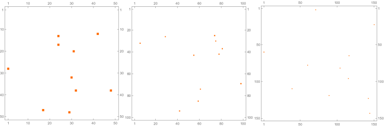
Figure 2: A numerical illustration of the limit (59). The red dots are positions on the lattice where the state is in the $|1\rangle$ state. From left to right we have $n^{\prime}=2.5\times 10^{3},10^{4},2.25\times 10^{4}$ respectively while $\lambda(x)$ is fixed to 1 (with $dV(x)=10$ to make the figures easier to read). It is clear that as $n^{\prime}\to\infty$ the expected number of excited states are approximately fixed.

Consider the fermionic systems on the sites inside the element $dV(x)$. We assume the $p(x)$ to be smooth enough so that in the small region $dV(x)$ it is approximately constant. The fermionic factors in the density matrix that comes from the region $dV(x)$ is

$$\bigotimes_{x\in dV(x)}\rho_{x}=\bigotimes_{x\in dV(x)}(1-p(x))|0\rangle_{x}\langle 0|+p(x)|1\rangle_{x}\langle 1|\ .$$ (61)

In the particle number basis in $dV(x)$ it reads

$$\rho_{dV(x)} =\bigotimes_{x\in dV(x)}\left((1-p(x))|0\rangle\langle 0|+p(x)|1\rangle\langle 1|\right)$$ (62)

$$=\left((1-p(x))|0\rangle\langle 0|+p(x)|1\rangle\langle 1|\right)^{n^{\prime}}$$ (63)

$$=P(n_{x}=k)\left(|0\rangle\langle 0|\right)^{\otimes(n^{\prime}-k)}\otimes\left(|1\rangle\langle 1|\right)^{\otimes k}\,,$$ (64)

where as above $n^{\prime}=ndV(x)$ is the total number of grid points in the volume element, $n_{x}$ is the total number of sites that are in the $|1\rangle$ states in the volume element $dV(x)$, equivalently it is the eigenvalue of the operator $\sum_{x\in dV(x)}N_{x}$. From this we read out the probability to have $n_{x}=k$ fermionic excitations in this volume is

$$P(n_{x}=k)={n^{\prime}\choose k}p(x)^{k}(1-p(x))^{n^{\prime}-k}\ .$$ (65)

In the limit (59), this probability becomes

$$\lim\limits_{n^{\prime}\to\infty}P_{dx}(n_{x}=k) =\frac{n^{\prime}!}{k!(n^{\prime}-k)!n^{\prime k}}(n^{\prime}p)^{k}(1-p)^{n^{\prime}-k}$$ (66)

$$=\frac{n^{\prime}!}{k!(n^{\prime}-k)!n^{\prime k}}(n^{\prime}p)^{k}(1-\frac{n^{\prime}p}{n^{\prime}})^{n^{\prime}-k}$$ (67)

$$=\frac{1}{k!}(\Lambda_{dx}(x))^{k}(1-\frac{\Lambda_{dx}(x)}{n^{\prime}})^{n^{\prime}}$$ (68)

$$=\frac{\Lambda_{dx}(x)^{k}}{k!}e^{-\Lambda_{dx}(x)}=P_{\text{Pois}}(\Lambda_{dx}(x),k)\ .$$ (69)

which means in the limit (59) the distribution of excitations in any open subset $dV(x)$ obeys a Poisson distribution.

Next we would like to trace over the Hilbert space of the spin degrees of freedom. For reasons discussed above, we consider the following trace

$$\text{Tr}_{{\cal H}}\left(\rho(-1)^{F}e^{-\beta H}\right)=\text{Tr}_{{\cal H}}\left(\rho e^{-\beta\left(H-\frac{i\pi}{\beta}F\right)}\right)=\text{Tr}_{{\cal H}}\left(\bigotimes_{dV(x)}\rho_{dV}\,e^{-\beta\sum_{x}\left(H_{x,0}+H_{x,1}-\frac{i\pi}{\beta}F_{x}\right)}\right)\,,$$ (70)

Because $e^{i\pi F}|n\rangle=e^{i\pi N}|n\rangle$ and the bosonic fields $\phi_{x}$ do not act on these fermionic component of the state (so they should be considered as functions in this computation), the $H_{x,1}$ and $F_{x}$ are diagonal on the states described by the density matrix. This together with (64), (65) and (69) reduces the trace to

$$\text{Tr}_{{\cal H}}\left(\bigotimes_{dV(x)}\rho_{dV}\,e^{-\beta\sum_{x}\left(H_{x}-\frac{i\pi}{\beta}F_{x}\right)}\right)=\text{Tr}_{{\cal H}}\left(\bigotimes_{dV(x)}\rho_{dV}\,e^{-\beta\sum_{x}\left(H_{x,0}+(m-\phi_{x}-\frac{i\pi}{\beta})N_{x}\right)}\right)$$ (71)

$$=\sum_{k_{x}=0}^{\infty}\left(\prod_{dV(x)}P_{\text{Pois}}(\Lambda_{dx}(x),n_{x}=k_{x})\right)e^{-\beta\sum_{dV(x)}\left(H_{x,0}dV(x)+k_{x}(m-\phi_{x}-\frac{i\pi}{\beta})\right)}$$ (72)

$$=e^{-\sum_{dV(x)}\left(\beta H_{x,0}dV(x)+\Lambda_{dx}(x)e^{-\beta\left((m-\phi)\right)}+\Lambda_{dx}(x)\right)}$$ (73)

where in the last line we have taken the continuous limit and we have also used (59) and

$$\sum_{n=0}^{\infty}\frac{\lambda^{n}}{n!}e^{-\lambda}e^{un+c}=e^{\lambda(e^{u}-1)+c}\ .$$ (74)

In addition, the discretization is fine enough so that the $\phi_{x}$ is approximately constant in each element $dV(x)$.

In addition, we notice that in the above derivation we did not specify any details about the decomposition of ${\cal M}$ into the countable sum of open sets $dV(x)$. First, it is trivial to show the existence of such decompositions since the lattice points are countable and each open set contains a large number of lattice points, we can therefore use any lattice point in a given open set $dV(x)$ to label it. Since all the open set are disjoint, there is no ambiguity, such as repeated labelling, in this process. This shows the existence of the decomposition. Second, the fact that the above derivation does not depend on the details of the decomposition simply means for different choices of the decomposition the result is always the same.

What we have done so far is to consider a special scaling limit (60) of a lattice system, where a Poisson process description of the system is available. To see this clearly, we start with (71) where we trace over the fermions. In the limit (59) this trace can be cast into the form of (72) where we show that the number of excited lattice point in subset $dV(x)$ are mutually independent since there is no fermionic hopping terms among different site. Furthermore the probability of $n_{x}$ in the mixed state represented by the density matrix (57) in the limit (60) is a Poisson distribution with Poisson parameter $\Lambda(x)$. These together mean that the limit can be described by a Poisson process with the $n_{x}$ being the counting measure (23) and the $n^{\prime}p(x)$ and $np(x)$ quantities in the special limit (60) being the mean measure and the intensity of the Poisson process. Therefore, as discussed in previous sections 2.2 and 2.1 this theory, in particular equation (71), can be considered as an ensemble of theories with a source $N_{x}$ that is related to a discrete Poisson distribution that is of the same type of the theory defined by (1) and (7). But on the other hand, the theory clearly has another microscopic description as explained in this section. This then setup an equivalence with the ensemble averaged Poisson random theory discussed in section 2.1 and section 2.2 and gives an explicit example that an ensemble average of theories could actually be equivalently an average of an ensemble of states in a single (microscopic) theory.

With this understanding, we actually do not have to do the above computation as in (71)-(LABEL:tr4), rather this is nothing but the Laplacian functional of a Poisson process where the mean measure is identified with the $\Lambda_{dx}(x)$ function in the continuum limit. Therefore we get an effective potential of the bosonic $\phi$ source function as

$${\cal H}(x)=\frac{\lambda(x)}{\beta}e^{-\beta\left(m-\phi\right)}+\frac{\lambda(x)}{\beta}=\frac{\lambda(x)}{\beta}e^{-\beta m}e^{\beta\phi_{x}}+\frac{\lambda(x)}{\beta}\ .$$ (75)

Defining

$$b=\frac{\beta}{2}\,,\qquad\mu=\frac{\lambda}{2\pi\beta}e^{-\beta m}=\frac{\lambda}{4\pi b}e^{-2bm}\,,$$ (76)

we find the effective potential to have the form of a (generalized) Liouville potential

$${\cal H}(x)=2\pi\mu(x)e^{2b\phi_{x}}+\frac{\lambda(x)}{2b}\ .$$ (77)

Notice that explicitly the Hamiltonian is not exactly of the Liouville form since now the $\mu$ is a function rather than a constant. This is similar with the results in the previous section 2.1 and 2.2. Again we defer a more detailed discussion of the position dependent case in section 5.3.

3.3 The low energy limit

Next we focus on the low energy modes which are expected to have a canonical kinetic term in continuous spacetime and are exactly described by a Liouville theory. This amounts to go to the frequency space and extract the effective action near zero momentum.

In the following, we consider the simplest case with 1 spatial dimension. Then the position label $x$ in $\phi_{x}$ is equivalently labelled by the order of the $\phi_{x}$ on the chain, namely $x=ja$ where $j\in\mathbb{Z}$ and $a$ is just a scale of the grid interval. Equivalently, we can use this $j$ index to label the different fields.

Our main consideration is on the following quadratic terms in (53)

$$H=\frac{m}{2}\sum_{j}\phi_{j}^{2}+\sum_{|j-k|=1}t_{jk}\phi_{j}\phi_{k}\,,$$ (78)

where

$$t_{ij}=t_{ji}\ .$$ (79)

For simplicity we consider a homogeneous chain so that the only non-vanishing hopping coupling is

$$t_{jj+1}=t\ .$$ (80)

It is well known that a change of variables

$$\phi_{k}\to\phi^{\prime}_{k}=\sqrt{\frac{1}{N+1}}\sum_{j}\sin\left(\frac{\pi(j+N+1)k}{2(N+1)}\right)\phi_{j}\,,\qquad k=1,\ldots,2N+1$$ (81)

diagonalizes the Hamiltonian (78). Furthermore, it is instructive to define a spatial momentum

$$p_{k}=\frac{k\pi}{2(N+1)a}\ .$$ (82)

In terms of this momentum the new field can be written as

$$\phi^{\prime}_{k}=\sqrt{\frac{1}{N+1}}\sum_{j}\sin\left(p_{k}(x_{j}-x_{0})\right)\phi_{j}\,,$$ (83)

where $x_{0}=-(N+1)a$. From this expression it is evident that the $p_{k}$ has the meaning of a momentum since the form of the change of variable (83) is in fact a discrete Fourier transform with the momentum space represented by $p_{k}$.

With this new variable the diagonalized Hamiltonian then reads

$$H=\sum_{k}\epsilon_{k}{\phi^{\prime}}_{k}^{2}\,,\qquad\epsilon_{k}=\frac{m}{2}-t\cos\left(\frac{k\pi}{2(N+1)}\right)=\frac{m_{\phi}}{2}-t\cos\left(p_{k}a\right)\ .$$ (84)

In the continuum limit $a\to 0,~{}Na\to\infty$, so that $p_{k}\to 0$, the dispersion relation becomes

$$\epsilon_{k}=\frac{m}{2}-t+\frac{t}{2}\left(p_{k}a\right)^{2}+{\cal O}(p_{k}^{4})\ .$$ (85)

In particular, if we choose

$$m=2m_{\phi}^{2}+2t\,,\qquad t=\frac{2}{c^{2}}a^{-2}\geq 0\,,\qquad m_{\phi}\,,a\,,c\in\mathbb{R}$$ (86)

with $c$ being a constant, we recover the dispersion relation

$$\epsilon_{k}=m_{\phi}^{2}+\frac{1}{c^{2}}p_{k}^{2}+{\cal O}(p_{k}^{4})\ .$$ (87)

Therefore, to the leading order we get with the simplification (80) and (86) we recover the spatial momentum term of a relativistic particle in a flat background. Explicitly, the Hamiltonian is

$$H_{sp} =\frac{1}{c^{2}}\sum_{k}p_{k}^{2}{\phi^{\prime}_{k}}^{2}$$ (88)

$$=\frac{1}{c^{2}}\sum_{k}p_{k}^{2}\left(\sqrt{\frac{1}{N+1}}\sum_{j}\sin\left(p_{k}(x_{j}-x_{0})\right)\phi_{j}\right)^{2}$$ (89)

$$=-\frac{1}{c^{2}(N+1)}\sum_{k=1}^{2N+1}\left(\sum_{j=-N}^{N}\sin\left(p_{k}(x_{j}-x_{0})\right)\phi_{j}\right)\partial_{x}^{2}\left(\sum_{j}\sin\left(p_{k}(x_{j}-x_{0})\right)\phi_{j}\right)$$ (90)

$$=-\frac{1}{c^{2}(N+1)}\partial_{x}^{2}\sum_{k}\sum_{j=-N}^{N}\sum_{r=-N}^{N}\sin\left(p_{k}(x_{j}-x_{0})\right)\sin\left(p_{k}(x_{r}-x_{0})\right)\phi_{j}\phi_{r}$$ (91)

$$=-\frac{1}{c^{2}(N+1)}\partial_{x}^{2}\sum_{j=-N}^{N}\sum_{r=-N}^{N}(N+1)\delta_{j,r}\phi_{j}\phi_{r}$$ (92)

$$=-\frac{1}{c^{2}}\sum_{j=-N}^{N}\phi_{x}\partial_{x}^{2}\phi_{x}=\frac{1}{c^{2}}\sum_{j=-N}^{N}\left(\partial_{x}\phi_{x}\right)^{2}$$ (93)

where we have used (83). In the third line we have regarded the $x_{j}$ formally as the discrete value of a continuous position coordinate with respect to which the $\partial_{x}$ operator is defined. It should be considered as the continuous limit of the difference operator.

Therefore together with (50), (52), (76), (77), (78) and (93), we get the following action for the low energy continuous limit of the theory obtained from tracing over the microscopic fermionic degrees of freedom

$$H=\sum_{x}\left(\pi_{x}^{2}+\frac{1}{c^{2}}\left(\partial_{x}\phi_{x}\right)^{2}+J_{0}(x)\phi_{x}+2\pi\mu(x)e^{2b\phi_{x}}+\frac{\lambda(x)}{2b}\right)\,,$$ (94)

where we have taken the $n\to\infty$ limit of (93). We find this is the Hamiltonian of the Liouville theory, similarly as that from averaging over a Poisson distributed random sources.

Further notice that in this derivation, we have tuned the parameters in the microscopic model so that in the continuum limit the scalar fields has a classical relativistic kinetic term on flat Euclidean spacetime. We could in fact consider more general parameters in the microscopic model, which will lead to a more general kinetic term.

4 Sinh-Gordon type models

In the previous example, the random source is drawn from a Poisson process which has the property that only positive values are supported in the distribution. One would ask if this discussion is only specific to the Poisson distribution or can be made more general. In addition, one would naturally ask what if we consider a distribution where the random variable can take both positive and negative (discrete) values, which is more similar to the Gaussian distribution. In the following we consider such a model from the random ensemble average point of view and the microscopic points of view. We will show that the average of this model leads to Sinh-Gordon type theories.

4.1 The random ensemble point of view

First, on the level of random average of different theories, we could consider a different Probability distribution of the source. For example, we can consider a similar model of

$${\cal L}=\partial_{\mu}\phi\partial^{\mu}\phi-\left(J_{0}(x)+J_{1}(x)\right)\phi\,,$$ (95)

where $J_{1}(x)$ is related to the Skellam distribution (146)

$$P(x;\mu_{1},\mu_{2})=e^{-(\mu_{1}+\mu_{2})}\left(\frac{\mu_{1}}{\mu_{2}}\right)^{x/2}I_{x}(2\sqrt{\mu_{1}\mu_{2}})\,,\qquad~{}~{}x\in\mathbb{Z}\,,$$ (96)

where $I_{x}$ is the modified Bessel function of the first kind and the $\mu_{1}$ and $\mu_{2}$ are parameters characterizing this random distribution

$$\langle J_{1}\rangle=\mu_{1}-\mu_{2}\,,\qquad\langle J_{1}^{2}\rangle-\langle J_{1}\rangle^{2}=\mu_{1}+\mu_{2}\,,\qquad\mu_{1},\mu_{2}\geq 0\ .$$ (97)

The random averaging can be done following the above Liouville discussion in either the more physical way discussed in section 2.1 or the more mathematical way in section 2.2. In the latter approach, the random sources can still be considered from a point process, the only difference is that now the probability distribution of the $N(B)$ for any open set on ${\cal M}$ is a Skellam distribution. Then following a similar discussions, we arrive at the solution with the following effective interaction Hamiltonian

$${\cal H}(x)=\frac{1}{\beta}\left(\mu_{1}(x)+\mu_{2}(x)+\mu_{1}(x)e^{\Phi}+\mu_{2}(x)e^{-\Phi}\right)$$ (98)

where $\mu_{1}(x)$ and $\mu_{2}(x)$ are two functions parametrizing the point process with the Skellam distribution measure on different open sets.

4.2 The microscopic point of view

As the above Poisson process case, there is again a microscopic setting which realizes the above theory as an average over an ensemble of microstates in a single theory. This provides another example showing that averaging over different theories could be understood as averaging over an ensemble of states within one theory in an appropriate limit.

Explicitly, we consider a microscopic model with again a grid of sites on which some fermionic quantum mechanical modes exist. We consider a simplest model with two complex fermions $\psi^{1}_{x}$ and $\psi^{2}_{x}$ on each site labelled by $x$. The interaction Hamiltonian of the collection of the fermionic systems reads

$$H_{x}(t) =\bar{\psi}^{1}_{x}(t)\psi^{1}_{x}(t)\phi_{x}(t)-\bar{\psi}^{2}_{x}(t)\psi^{2}_{x}(t)\phi_{x}(t)\ .$$ (99)

Notice that there is a relative minus sign between the two terms, this reflects the fact that we assign opposite counting charges of the two fermions under the particle number operator, mimicking the electron-hole pair in more familiar systems.

One can again consider the microstates to be in an ensemble represented by a factorized density matrix

$$\rho_{\psi}=\rho_{\psi^{1}}\otimes\rho_{\psi^{2}}\,,$$ (100)

where

$$\rho_{\psi^{i}}=\bigotimes_{x,i}\rho_{x,i}\,,\qquad\rho_{x,i}=(1-p_{i}(x))|0\rangle_{x,i}\langle 0|+p_{i}(x)|1\rangle_{x,i}\langle 1|\ .$$ (101)

Here we emphasize again that this is only a special mixed state that we choose the microscopic fermions to stay in. The system could very well be in a different mixed states, and in those cases the effective theory of $\phi$ could be very different.

The Hamiltonian is closed related to the “net” number operator

$$M_{x}=\bar{\psi}^{1}_{x}\psi^{1}_{x}-\bar{\psi}^{2}_{x}{\psi}^{2}_{x}\,,$$ (102)

which satisfies

$$M_{x}|0\rangle_{x,i}=0\,,\qquad M_{x}|1\rangle_{x,i}=(3-2i)|1\rangle_{x,i}\ .$$ (103)

Next we would like to consider the “continuum limit” in the same sense as the in previous Liouville discussion in section 3

$$n\to\infty\,,$$ (104)

where $n$ is the total number of lattice points per unit volume. Concretely, we again assume $p_{i}(x)$ to be smooth enough so that in the small region $dV(x)$ it is approximately a constant, so we consider the limit

$$\lim\limits_{n^{\prime}\to\infty}n^{\prime}p_{i}(x)=\Lambda_{i,dV}(x)\,,$$ (105)

and similarly

$$\Lambda_{i,dV}(x)=\mu_{i}(x)dV(x)\,,\qquad\mu_{i}(x)\sim{\cal O}(1)\ .$$ (106)

Once again, we could consider $\Lambda_{i,dV}(x)$ as an induced measure on the carrier space ${\cal M}=\mathbb{R}^{d}$.

Then the probability of the total net excitation in this volume element $dV(x)$ being $m_{dV}=k$ with $k>0$ is

$$P(m_{dV}=k)=\sum_{n_{2}=\max(0,-k)}^{\infty}P(n_{1}-n_{2}=k)$$ (107)

$$=\sum_{n_{2}=\max(0,-k)}^{\infty}{n^{\prime}\choose n_{2}+k}p_{1}(x)^{n_{2}+k}(1-p_{1}(x))^{n^{\prime}-n_{2}-k}{n^{\prime}\choose n_{2}}p_{2}(x)^{n_{2}}(1-p_{2}(x))^{n^{\prime}-n_{2}}\,,$$ (108)

which can be simply counted using the fact that the systems on each sites are independents. We have also only computed the $k>0$ case, for $k<0$, we can rewrite the sum in terms of $n_{1}=n_{2}+k$ and the result is the same as $P(m_{dV}=-k)$.

In the limit (105), the above probability becomes

$$\lim\limits_{n^{\prime}\to\infty}P(m_{dV}=k)$$ (109)

$$=\sum_{n_{2}=\max(0,-k)}^{\infty}\frac{\Lambda_{1,dV}(x)^{n_{2}+k}}{(n_{2}+k)!}e^{-\Lambda_{1,dV}(x)}\frac{\Lambda_{2,dV}(x)^{n_{2}}}{(n_{2})!}e^{-\Lambda_{2,dV}(x)}$$ (110)

$$=\sum_{n_{2}=\max(0,-k)}^{\infty}P_{\text{Pois}}(\Lambda_{1,dV}(x),n_{2}+k)P_{\text{Pois}}(\Lambda_{2,dV}(x),n_{2})$$ (111)

$$=e^{-(\Lambda_{1,dV}(x)+\Lambda_{2,dV}(x))}\left(\frac{\Lambda_{1,dV}(x)}{\Lambda_{2,dV}(x)}\right)^{k/2}I_{k}(2\sqrt{\Lambda_{1,dV}(x)\Lambda_{2,dV}(x)})\,,$$ (112)

where $I_{k}(x)$ is the modified Bessel function of the first kind. For $k<0$ we follow the same procedure, and the result can be put into a uniform expression for all values of $k$

$$\lim\limits_{n^{\prime}\to\infty}P(m_{dV}=k):=P_{\text{Sk}}(\Lambda_{1,dV}(x),\Lambda_{2,dV}(x),k)$$ (113)

$$\quad=e^{-(\Lambda_{1,dV}(x)+\Lambda_{2,dV}(x))}\left(\frac{\Lambda_{1,dV}(x)}{\Lambda_{2,dV}(x)}\right)^{k/2}I_{k}(2\sqrt{\Lambda_{1,dV}(x)\Lambda_{2,dV}(x)})\ .$$ (114)

This probability on the open set $dV(x)$ is nothing but the Skellam distribution with the mean value $\Lambda_{1,dV}(x)-\Lambda_{1,dV}(x)$ and the variance $\Lambda_{1,dV}(x)+\Lambda_{1,dV}(x)$, both depending on the position $x$ and the open set $dV(x)$.

Next we would like to trace over the Hilbert space of the Fermi system, which is equivalent to integrating out the spin system background. We again consider the following trace

$$\text{Tr}_{{\cal H}}\left(\rho(-1)^{F}e^{-\beta H}\right)=\text{Tr}_{{\cal H}}\left(\rho e^{-\beta\left(H-\frac{i\pi}{\beta}F\right)}\right)=\text{Tr}_{{\cal H}}\left(\bigotimes_{dV(x)}\rho_{x}e^{-\beta\sum_{dV}\left(H_{dV(x)}-\frac{i\pi}{\beta}F_{dV(x)}\right)}\right)\,,$$ (115)

which follows from a similar derivation as in the previous Liouville theory case. For simplicity we drop the terms that only depend on the bosonic field. As shown in the previous case, those terms do not affect the evaluation of the trace and can be put back at the end. The evaluation of this trace reads

$$\text{Tr}_{{\cal H}}\left(\bigotimes_{dV(x)}\rho_{x}e^{-\beta\sum_{dV}\left(H_{dV(x)}-\frac{i\pi}{\beta}F_{dV(x)}\right)}\right)$$ (116)

$$=\sum_{k_{x}}\left(\prod_{dV(x)}P_{\text{Sk}}(\Lambda_{1,dV}(x),\Lambda_{2,dV}(x),k)e^{-\beta\sum_{dV(x)}\left(k(m+\phi_{x}-\frac{i\pi}{\beta})\right)}\right)$$ (117)

$$=e^{\sum_{dV(x)}\left(\Lambda_{1,dV}(x)\left(-e^{-\beta\left((m+\phi)\right)}-1\right)+\Lambda_{2,dV}(x)\left(-e^{\beta\left((m+\phi)\right)}-1\right)\right)}$$ (118)

$$=e^{-\beta{\bigintssss}dx\left(\frac{\mu_{1}(x)}{\beta}e^{-\beta\left(m+\phi\right)}+\frac{\mu_{2}(x)}{\beta}e^{\beta\left(m+\phi\right)}+\frac{\mu_{1}(x)}{\beta}+\frac{\mu_{2}(x)}{\beta}\right)}\,,$$ (119)

where we have used $e^{i\pi F}|n_{1},n_{2}\rangle=e^{i\pi(n_{1}+n_{2})}|n_{1},n_{2}\rangle=e^{i\pi(|n_{1}-n_{2}|)}|n_{1},n_{2}\rangle$ and also we have adopted the identification of $\Lambda_{i,dx}(x)=\mu_{i}(x)dx$ as an induced measure to rewrite the weighted sum in the exponential into an integral over ${\cal M}$ with a dynamical measure.

We thus find the resulting Hamiltonian is of the form of a Sinh-Gordon type potential. We can follow the same treatment in the previous section 3 to show the emergence of a relativistic kinetic terms and obtain the full Hamiltonian of the Sinh-Gordon action.

5 Discussion

In this section we discuss some interesting questions and extensions related to the material in the above main text.

5.1 Relation to Gaussian randomness

Focusing on discrete distributions is a crucial difference between this work and the previous literature on ensemble averages of continuous Gaussian type random variables. It is often the case that a further limit of the discrete distribution, for example the Poisson distribution that we mainly discussed here, gives a Gaussian distribution, which is guaranteed by the central limit theorem as long as the events that the distribution describes are mutually independent. Therefore we can also regard the discussion in this paper as a first attempt towards refining the results in previous Gaussian random (holographic) theories, including SYK type models and the random matrix theories, in the sense of reverting the limit to go back from Gaussian to discrete distributions.

5.2 The quantum mechanics dual description

We can also integrate out the $\phi_{x}$ fields and ask what does the resulting microscopic model look like. We expect the result, which is a 0+1d quantum mechanical model with $x$ being discrete flavour labels of the fermions, to be a purely field theoretical description of the same system.

Explicitly, it is easier to work in the Lagrangian formalism, where the coupled theory is defined as

$$L^{E}=\sum_{x}\left(\frac{1}{2}\dot{\phi_{x}}^{2}+\frac{m_{\phi}}{2}\phi_{x}^{2}+\frac{t_{x-1,x}}{2}\phi_{x-1}\phi_{x}+\frac{t_{x,x+1}}{2}\phi_{x}\phi_{x+1}+i\bar{\psi}\dot{\psi}+m\bar{\psi}_{x}\psi_{x}-\bar{\psi}_{x}\psi_{x}\phi_{x}\right)\ .$$ (120)

Notice that in this section we again work in Euclidean signature. Treating $x$ as a flavour index, we can integrate out the $\phi_{x}$ to get

$$e^{-\int dtL^{E}_{eff}} =\int{\cal D}\phi_{x}e^{-\int dtL^{E}}\sim e^{-\frac{1}{2}\log(M)+\int dt\left(i\bar{\psi}\dot{\psi}+m\bar{\psi}_{x}\psi_{x}+\frac{1}{2}\bar{\psi}_{x}\psi_{x}\bar{\psi}_{y}\psi_{y}(M^{-1})_{xy}\right)}\,,$$ (121)

where $\sim$ simply means up to an irrelevant constant and the matrix $M$ is defined to be

$$M_{xy}=-\partial^{2}_{\tau}\delta_{x,y}+m_{\phi}\delta_{x,y}+t_{x-1,x}\delta_{y,x-1}+t_{x,x+1}\delta_{y,x+1}\ .$$ (122)

We observe that the quantum mechanical description of the same model is characterized by a complex fermion system with a “nearest neigh bore” charge-charge coupling.

We can further consider the $M^{-1}$ factor as the coupling constants of the charge-charge interaction. This interaction can be analysed by a derivative expansion of the inverse of (122). In particular, the leading term in this expansion is simply the inverse of (122) with the derivative term turned off. The next-to-leading term is a 2-derivative term, which is irrelevant in the quantum mechanics system. As a result, for the purpose of obtaining an low energy effective theory we can simply drop all the derivative corrections to get the following effective action

$$S_{\text{eff}}=-\int dt\left(i\bar{\psi}\dot{\psi}+m\bar{\psi}_{x}\psi_{x}+\frac{1}{2}g_{xy}\bar{\psi}_{x}\psi_{x}\bar{\psi}_{y}\psi_{y}\right)\,,$$ (123)

where

$$g_{xy} =\left(m_{\phi}\delta_{x,y}+t_{x-1,x}\delta_{y,x-1}+t_{x,x+1}\delta_{y,x+1}\right)^{-1}\ .$$ (124)

We can again consider the special value (79) and (80) where the inverse can be computed as

$$g_{xy} =\left(m_{\phi}\delta_{x,y}+t\delta_{y,x-1}+t\delta_{y,x+1}\right)^{-1}$$ (125)

$$=\frac{1}{m_{\phi}}\sum_{k=0}\left(\frac{-t}{m_{\phi}}(\delta_{y,x-1}+\delta_{y,x+1})\right)^{k}$$ (126)

$$=\frac{1}{m_{\phi}}\sum_{k=0}\left(\frac{-t}{m_{\phi}}\right)^{k}\sum_{j=0}^{k}{k\choose j}\delta_{y,x+k-2j}\ .$$ (127)

Clearly $g_{xy}=g_{yx}$ so we can focus on $y\geq x$ cases where the sum over $j$ reduces to half of the range

$$g_{xy} =\frac{1}{m}\sum_{k=0}\left(\frac{-t}{m}\right)^{k}\sum_{j=0}^{\lfloor\frac{k}{2}\rfloor}{k\choose j}\delta_{y,x+k-2j}$$ (128)

$$=\frac{1}{m}\sum_{k=0}\left(\frac{-t}{m_{\phi}}\right)^{2k}\sum_{j=0}^{k}{2k\choose j}\delta_{y,x+2k-2j}+\frac{1}{m}\sum_{k=0}\left(\frac{-t}{m}\right)^{2k+1}\sum_{j=0}^{k}{2k+1\choose j}\delta_{y,x+2k+1-2j}$$ (129)

$$=\frac{1}{m}\sum_{p=0}^{\infty}\sum_{k=p}^{\infty}\left(\frac{-t}{m}\right)^{2k}{2k\choose k-p}\delta_{y,x+2p}+\frac{1}{m}\sum_{p=0}^{\infty}\sum_{k=p}^{\infty}\left(\frac{-t}{m}\right)^{2k+1}{2k+1\choose k-p}\delta_{y,x+2p+1}$$ (130)

$$=\frac{1}{m}\sum_{p=0}^{\infty}\sum_{k=0}^{\infty}\left(\frac{-t}{m}\right)^{2k+2p}{2k+2p\choose k}\delta_{y,x+2p}+\frac{1}{m}\sum_{p=0}^{\infty}\sum_{k=p}^{\infty}\left(\frac{-t}{m}\right)^{2k+2p+1}{2k+2p+1\choose k}\delta_{y,x+2p+1}$$ (131)

$$=\frac{1}{m\sqrt{1-\frac{4t^{2}}{m^{2}}}}\sum_{p=0}^{\infty}\left(\frac{\left(\frac{2t}{m}\right)^{2p}}{\left(\sqrt{1-\frac{4t^{2}}{m^{2}}}+1\right)^{2p}}\delta_{y,x+2p}-\frac{\left(\frac{2t}{m}\right)^{2p+1}}{\left(\sqrt{1-\frac{4t^{2}}{m^{2}}}+1\right)^{2p+1}}\delta_{y,x+2p+1}\right)\ .$$ (132)

Adding back the $y<x$ terms, we simply get

$$g_{xy}=\frac{1}{m\sqrt{1-\frac{4t^{2}}{m^{2}}}}\sum_{p=-\infty}^{\infty}\left(\frac{\left(\frac{2t}{m}\right)^{2|p|}}{\left(\sqrt{1-\frac{4t^{2}}{m^{2}}}+1\right)^{2|p|}}\delta_{y,x+2p}-\frac{\left(\frac{2t}{m}\right)^{2|p|+1}}{\left(\sqrt{1-\frac{4t^{2}}{m^{2}}}+1\right)^{2|p|+1}}\delta_{y,x+2p+1}\right)\ .$$ (133)

For the special value (86), the parameter in the above result behaves as

$$\frac{t}{m}=\frac{1}{2(1+\frac{m_{\phi}^{2}}{t})}\leq\frac{1}{2}\ .$$ (134)

In this range, the coupling considered above is in general real and positive. However, when the inequality is saturated, the coupling actually diverges.

The physical reason of this divergence is clear. When the inequality saturates $m_{\phi}=0$ according to (86), so the effective mass of the infrared $\phi$ mode vanishes. When this happens, integrating out this massless modes is inconsistent and leads to divergences. What we have observed is just a realization of this well known phenomenon, see e.g. Seiberg:1994bz ; Seiberg:1994rs in our very simple model, where no gauge symmetry or supersymmetry is involved.

Further notice that the results in this section are simplified version due to the assumption (79) and (80). Without these assumptions we expect to get richer structure of this dual description.

5.3 Interpretation as emergent gravity ?

From the results of the previous sections, we observe that Liouville theory and generalizations could arise from averaging over an ensemble of theories with random sources. The latter type of theories could have a microscopic origin where one traces over a set of underlying fermionic degrees of freedom in a specific state to generate an effective theory of the rest degrees of freedom. In both the two scenarios a key point is that by relating such averaging or tracing out the microscopic degrees of freedom to the mathematical description of (Poisson) point processes, an emergent probabilistic measure on the carrier space naturally appears. One is then tempting to identify such an emergent measure, which ultimately comes from tracing over the fermionic microstates, with a geometric metric which facilitates an emergent gravity theory whose action takes the form of Liouville action.

This does not sound that unreasonable given that the 2D Liouville theory itself does emerge from the response of the conformal matter fields to a Weyl transformation of the background metric, see e.g. DHoker:1990prw . The only difference in our setting is that we do not start with a conformal matter fields that couples to a gravitational background. Instead we start from a large number of microscopic fermionic modes that couples to a bosonic mode, then in a double-scaled continuous limit an effective Liouville action emerges for the bosonic modes.

Concretely, recall that the effective action of the Liouville theory can be obtained from the response of the matter field to a Weyl transformation of the metric $h_{\mu\nu}\to e^{\phi}h_{\mu\nu}$, with the effective action

$$I_{\mathrm{L}}^{(b)}=\frac{1}{4\pi}\int\mathrm{d}^{2}x\sqrt{|h|}\left(Q\Phi(x)R_{h}(x)+(\nabla\Phi)^{2}+4\pi\mu e^{2b\Phi(x)}\right)\,,$$ (135)

where $\mu$ is a cosmological constant and $Q$ is a background charge related to the property, such as the central charge, of the matter fields.

In our analysis, the effective action of the free scalar theory with a Poisson random source has been shown (21) to be

$$S_{\text{eff}}=\int d^{d}x\left(\partial_{\mu}\phi\partial^{\mu}\phi(x)-J_{0}(x)\phi+\lambda(x)(e^{\phi(x)}-1)\right)\ .$$ (136)

Given the resemblance of the two actions, we would like to try matching the two actions by identifying the dilaton $\Phi$ in (135) with the boson $\phi$ in (21) for $d=2$. However, given the form of the two actions, it is the simplest if we fix a gauge of the gravitational theory with dynamical metric field $h_{\mu\nu}$. This can be directly observed from a simple comparison: fluctuations of the metric, not only its determinant, is dual to a change of the kinetic term that can be traced to a different hopping structure on the microscopic lattice. Thus choosing a different hopping structure on the lattice correspond to a change of the metric. Fixing the metric to a certain gauge is them mapped to a choice of the hopping terms on the lattice. For example, for the choice of the hoppings we discussed above, the effective kinetic term is simply the Laplacian on the conformally flat spacetime. To make the comparison transparent, we fix the metric in (135) to the conformal gauge

$$h_{\mu\nu}=e^{\rho(x)}\delta_{\mu\nu}\ .$$ (137)

In this gauge, the above duality simplifies to

$$-Q\delta^{\mu\nu}\partial_{\mu}\partial_{\nu}\rho(x)=-J_{0}(x)$$ (138)

$$4\pi\mu e^{\rho(x)}=2\pi\mu(x)=\frac{\lambda(x)}{2b}e^{-2mb}$$ (139)

$$\delta^{\mu\nu}\partial_{\mu}\partial_{\nu}=\delta^{\mu\nu}\partial_{\mu}\partial_{\nu}\ .$$ (140)

The third line reduces to an identity as a result of our fixing the gauge (137), while the first two equations implies a condition between the canonical source $J_{0}(x)$ and the $\lambda(x)$ that can either be understood as the “parameter” characterizing the point process or characterizing the state of in which the effective action describes in the microscopic ensemble average description. In particular, the relation is

$$\frac{J_{0}(x)}{Q}=\delta^{\mu\nu}\partial_{\mu}\partial_{\nu}\log\left(\frac{\lambda(x)e^{-2mb}}{8\pi\mu b}\right)=\delta^{\mu\nu}\partial_{\mu}\partial_{\nu}\log\left(\lambda(x)\right)\,,$$ (141)

where in the last expression we have assumed that all the other parameters in the microscopic setting are independent of $x$.

This is a very interesting relation stating that we can consider the $J_{0}$ as also the source of the $\log(\lambda(x))$ when the latter is regarded as a classical field. This means for a given $J_{0}(x)$ the value of the function $\lambda(x)$ is determined once a boundary condition is provided. Microscopically, this relation has a clearer interpretation: for any given $J_{0}(x)$ the microscopic state in which the system has a gravitational description can be identified so that the density matrix of the state (57) scales correctly (59) so that the limiting $\lambda(x)$ function should satisfies the condition (141). This agrees with the general philosophy of gauge/gravity duality where the content of the duality depends crucially on which states the quantum field theory is in. It is true that the limit (59) and the condition (141) can not isolate a single state in the microscopic theory. But this is also as what we would expect since in our picture the different states giving the same limit (59) is not distinguishable from the semi-classical gravity interpretation. It is likely that the different states with the same (59) carries information about quantum corrections to the classical gravity/geometry. We plan to understand this proposal better in the future.

Further notice that the requirement of a gravitational interpretation only fix the shape dependence of $J_{0}(x)$ on $\lambda(x)$, the size of the $J_{0}(x)$ field can however vary and it is proportional to $Q$ in the gravity interpretation. We know that in the derivation of the Liouville theory as a response of matter fields to a Weyl transformation of the gravity background they couple to, $Q$ roughly counts the number of degrees of freedom of the matter fields, and hence an indication of the strength of the matter coupling. In our derivation, the $\phi(x)$ scalar field can be interpreted as the dilaton in the 2d gravity of the Liouville type, and then the size of $J_{0}(x)$ can thus be understood as the strength of the coupling to some other matter field that could be considered as other conformal matters fields in the gravity interpretation.

Of course this identification and interpretation are specialized in the conformal gauge (137). It is definitely an interesting question to set up a concrete relation covariantly. One simple idea is that one should be able to impose conditions on the allowed probability measure $\Lambda(dx)=\lambda(x)dV(x)$ so that there is an emergent diffeomorphism on the $\lambda(x)$ that can be identified with the diffeomorphism in the gravity description But this is beyond the scope of this paper and we will discuss this in more details in future work. Nevertheless, in either respect, namely either our result being gauge dependence or in the near future we consider diffeomorphism invariant $\lambda(x)$ measure as the effective background metric, our construction and in particular the interpretation of emergent gravity is not forbidden by the Weinberg-Witten theorem.

Finally, we notice that connection between dilaton gravity models and the Liouville-type theory have been discussed recently Maldacena:2016hyu ; Bagrets:2016cdf ; Bagrets:2017pwq ; Mertens:2017mtv ; Mertens:2020hbs ; Maxfield:2020ale and similar discussion about the relation between the dilaton gravity theory with the sinh-Gordon and other types of theory StanfordSeiberg ; Mertens:2020hbs ; Witten:2020wvy . There have also been some discussions about the connection between 1d Liouville and the Schwarzian theory. In the paper Bagrets:2016cdf ; Bagrets:2017pwq , the author considered a rewriting of the Schwarzian theory as a Liouville theory with some regularization. In Mertens:2017mtv an indirect connection between the two theories are made via the reduction from integrating in and out different Lagrangian multiplier fields.

5.4 Concluding remarks

In this paper, we consider averaging over theories with discrete probability distribution, and show an explicit equivalence between this type of theories with the effective theory from tracing over part of the microscopic degrees of freedom of a single theory in some appropriate limit. Further notice that in this discussion, especially from the point of view of the Poisson point process, the spatial dimension of the carrier space is not crucial. Therefore it is possible to compare the above approach to some other known random deformations of free field theories in higher dimensions  Berkooz:2016cvq ; Murugan:2017eto ; Berkooz:2017efq ; Bulycheva2017 ; Peng:2018zap ; Ahn:2018sgn ; cepm .

While finishing the paper, we noticed other discussions of probabilistic construction of Liouville conformal field theory 2020arXiv200511530G . The approach there is very different from ours; there the Liouville field itself is considered as a random field under a specific probability measure. In our analysis in section 2.1 and 2.2, we only consider the source to be related to Poisson process, while the field $\phi(x)$ itself is conventional. So at the moment we have not observed any direct connection between our analysis and the approach used in 2020arXiv200511530G and the reference therein. It will be interesting to better understand possible connections in the future.

Acknowledgments

We thank Eduardo Casali, Chi-Ming Chang, Liangyu Chen, Sean Colin-Ellerin, Temple He, Veronika Hubeny, Yang Lei, Yan Liu, Mukund Rangamani, Ya-Wen Sun, Jia Tian, Huajia Wang, Jieqiang Wu, Yingyu Yang, Zekai Yu, Zhixian Zhu and other members at KITS for many interesting discussions on related topics. The work is supported by funds from the Kavli Institute for Theoretical Science (KITS) and a startup funding from the University of Chinese Academy of Science (UCAS), this work is also supported in part by the U.S. Department of Energy grant DE-SC0019480 under the HEP-QIS QuantISED program and by funds from the University of California.

Appendix A Discrete distributions

For the convenience of later computation it is useful to first list some properties of the distributions discussed in the main text.

$\bullet$ The Poisson distribution has the probability mass function

$$P(x,\lambda)=e^{-\lambda}\frac{\lambda^{x}}{x!}\Theta(x)\,,\qquad x\in\mathbb{Z}\,,$$ (142)

where

$$\Theta(x)=\begin{cases}1\,,\qquad x\geq 0\\ 0\,,\qquad x<0\end{cases}\ .$$ (143)

Its moment generating function (MGF) and characteristic function (CF) are

$$\text{MGF}: M_{x}(\Phi)=\mathbb{E}[e^{\Phi x}]=\sum_{-\infty}^{\infty}P(x,\lambda)e^{\Phi x}=e^{\lambda e^{\Phi}-\lambda}$$ (144)

$$\text{CF}: C_{x}(\Phi)=\mathbb{E}[e^{i\Phi x}]=\sum_{-\infty}^{\infty}P(x,\lambda)e^{i\Phi x}=e^{\lambda e^{i\Phi}-\lambda}\,,$$ (145)

where $\mathbb{E}$ is the mean value of the distribution assuming the random variable to be $x$.

$\bullet$ The Skellam distribution skellam has the probability mass function

$$P(x;\mu_{1},\mu_{2})=e^{-(\mu_{1}+\mu_{2})}\left(\frac{\mu_{1}}{\mu_{2}}\right)^{x/2}I_{x}(2\sqrt{\mu_{1}\mu_{2}})\,,\qquad x\in\mathbb{Z}\,,$$ (146)

where $I_{k}(x)$ is the modified Bessel function of the first kind. The MGF and CF are

$$\text{MGF}: M_{x}(\Phi)=\mathbb{E}[e^{\Phi x}]=\sum_{-\infty}^{\infty}P(x,\mu_{1},\mu_{2})e^{\Phi x}=e^{-(\mu_{1}+\mu_{2})+\mu_{1}e^{\Phi}+\mu_{2}e^{-\Phi}}$$ (147)

$$\text{CF}: C_{x}(\Phi)=\mathbb{E}[e^{i\Phi x}]=\sum_{-\infty}^{\infty}P(x,\mu_{1},\mu_{2})e^{i\Phi x}=e^{-(\mu_{1}+\mu_{2})+\mu_{1}e^{i\Phi}+\mu_{2}e^{-i\Phi}}\ .$$ (148)

To understand better the meaning of the Skellam distribution we consider two independent Poisson distributions $P(x_{1},\mu_{1})$ and $P(x_{2},\mu_{2})$. Then the joint distribution is

$$P(x_{1},\mu_{1})P(x_{2},\mu_{2})=e^{-\mu_{1}}\frac{\mu_{1}^{x_{1}}}{m_{1}!}e^{-\mu_{2}}\frac{\mu_{2}^{x_{2}}}{x_{2}!}\ .$$ (149)

It is easier to consider directly the generating function

$$G(z;\lambda)=\sum_{x=-\infty}^{\infty}P(x,\lambda)z^{x}\ .$$ (150)

For the current Poisson distribution, this gives

$$G(z;\lambda)=\sum_{x=0}^{\infty}e^{-\lambda}\frac{\lambda^{x}}{x!}z^{x}=e^{\lambda z-\lambda}\ .$$ (151)

Then the above joint distribution (149) is simply the $z_{1}^{x_{1}}z_{2}^{x_{2}}$ coefficient of

$$G(z_{1},z_{2};\lambda_{1},\lambda_{2})=G(z_{1};\lambda_{1})G(z_{2};\lambda_{2})=e^{\lambda_{1}(z_{1}-1)+\lambda_{2}(z_{2}-1)}=e^{-(\lambda_{1}+\lambda_{2})+(\lambda_{1}z_{1}+\lambda_{2}z_{2})}\ .$$ (152)

Consider the special case

$$z_{2}=\frac{1}{z_{1}}\,,$$ (153)

where the generating function becomes

$$G(z_{1},\frac{1}{z_{1}};\lambda_{1},\lambda_{2})=e^{-(\lambda_{1}+\lambda_{2})+(\lambda_{1}z_{1}+\lambda_{2}z_{1}^{-1})}=e^{-(\lambda_{1}+\lambda_{2})+\sqrt{\lambda_{1}\lambda_{2}}\left(\sqrt{\frac{\lambda_{1}}{\lambda_{2}}}z_{1}+{\left(\sqrt{\frac{\lambda_{1}}{\lambda_{2}}}z_{1}\right)}^{-1}\right)}\ .$$ (154)

The coefficient of $z_{1}^{x}$ in the above generating function leads to the Skellam distribution. To see this, we make use of the summation identity

$$e^{\frac{1}{2}z\left(t+t^{-1}\right)}=\sum_{m=-\infty}^{\infty}t^{m}I_{m}(z)\,,$$ (155)

to rewrite the generating function

$$G(z_{1},\frac{1}{z_{1}};\lambda_{1},\lambda_{2}) =e^{-(\lambda_{1}+\lambda_{2})+\sqrt{\lambda_{1}\lambda_{2}}\left(\sqrt{\frac{\lambda_{1}}{\lambda_{2}}}z_{1}+{\left(\sqrt{\frac{\lambda_{1}}{\lambda_{2}}}z_{1}\right)}^{-1}\right)}$$ (156)

$$=e^{-(\lambda_{1}+\lambda_{2})}\sum_{x=-\infty}^{\infty}\left(\sqrt{\frac{\lambda_{1}}{\lambda_{2}}}z_{1}\right)^{x}I_{x}(2\sqrt{\lambda_{1}\lambda_{2}}).$$ (157)

The coefficient of $z^{x}$ is precisely the Skellam distribution (146). This gives a clear meaning of the Skellam distribution; it is the distribution of the difference of two separate Poisson random variables.

With this result, we can proceed to compute the MGF and CF, for this we consider

$$M_{x}(\Phi) =\sum_{-\infty}^{\infty}P(x,\mu_{1},\mu_{2})e^{\Phi x}$$ (158)

$$=e^{-(\mu_{1}+\mu_{2})}\sum_{-\infty}^{\infty}\left(\frac{\mu_{1}}{\mu_{2}}\right)^{x/2}I_{x}(2\sqrt{\mu_{1}\mu_{2}})e^{\Phi x}$$ (159)

$$=e^{-(\mu_{1}+\mu_{2})}\sum_{-\infty}^{\infty}\left(\frac{\mu_{1}}{\mu_{2}}e^{2\Phi}\right)^{x/2}I_{x}(2\sqrt{\mu_{1}\mu_{2}})$$ (160)

$$=e^{-(\mu_{1}+\mu_{2})+\sqrt{\mu_{1}\mu_{2}}\left(e^{\Phi}\sqrt{\frac{\mu_{1}}{\mu_{2}}}+{\left(e^{\Phi}\sqrt{\frac{\mu_{1}}{\mu_{2}}}\right)}^{-1}\right)}$$ (161)

$$=e^{-(\mu_{1}+\mu_{2})+\mu_{1}e^{\Phi}+\mu_{2}e^{-\Phi}}\ .$$ (162)

The derivation for the CF is similar; one only needs to substitute $\Phi\to i\Phi$.

Appendix B A meaningless averaging scheme

In Euclidean signature, we try to get an effective action from

$$e^{-S_{\text{eff}}} =\sum_{J_{1}=0}^{\infty}P(J_{1},\lambda_{1})e^{-S}\,,$$ (163)

where

$$S=\int d^{d}x\,{\cal L}\ .$$ (164)

If we naively consider the measure $P(J_{1},\lambda_{1})$ to be the Poisson distribution function of the random variable $J_{1}$ at each point $x$, the average over the random source is

$$\int{\cal D}J_{1}\sum_{J_{1}(x)=0}^{\infty}P(J_{1}(x),\lambda_{1}(x))e^{\int d^{d}xJ_{1}(x)\phi(x)}\ .$$ (165)

To understand how to perform this average, we first consider discretizing the spacetime so that the above expression reduces to

$$\left(\prod_{n}\sum_{J_{1}(x_{n})=0}^{\infty}P\left(J_{1}(x_{n}),\lambda_{1}(x_{n})\right)\right)e^{\Delta x^{d}\sum_{n}J_{1}(x_{n})\phi(x_{n})}$$ (166)

$$=\left(\prod_{n}\sum_{J_{1}(x_{n})=0}^{\infty}P\left(J_{1}(x_{n}),\lambda_{1}(x_{n})\right)\right)\left(\prod_{n}e^{J_{1}(x_{n})\phi(x_{n})\Delta x^{d}}\right)\ .$$ (167)

where $n$ collectively denote the position of a point in the discretized lattice. Here we treat the sources on each individual lattice point to be independent of each other, which is the reason we take a product over the $n$ lattice points. On each point $x_{n}$ we sum over all possible values of the sources $J_{1}(x_{n})$. The product is

$$=\prod_{n}\left(\sum_{J_{1}(x_{n})=0}^{\infty}P\left(J_{1}(x_{n}),\lambda_{1}(x_{n})\right)e^{J_{1}(x_{n})\phi(x_{n})\Delta x^{d}}\right)$$ (168)

$$=\prod_{n}\left(e^{\lambda_{1}(x_{n})(e^{\phi(x_{n})\Delta x^{d}}-1)}\right)=e^{\sum_{n}\lambda_{1}(x_{n})(e^{\phi(x_{n})\Delta x^{d}}-1)}\,,$$ (169)

where in the second line we have used the sum over the Poisson distribution for any fixed $x_{n}$ (144); this is just the standard expression for the Laplace transform of the Poisson distribution with the parameter $\lambda(x_{n})$. However, the result of this direct computation looks strange since the $\Delta^{d}x$ is further on the shoulder of an extra exponential. This result is difficult to interpret; especially it is not clear how to take it’s continuous limit.

Comparing the derivation in this appendix with the results in section 2.1, we find the crucial difference between the naive random average and the Poisson process is that in the latter case the quantity that obeys the Poisson distribution is the measure on the carrier space, rather than the “rate of event” $J_{1}(x)$.

Appendix C More about the Poisson process

C.1 Random points versus counting measures

The notion of Poisson process has at least two interpretations. One is similar to the arrival process, like the time at which a bus comes to a bus stop, where it is really considered as a process or a sequence. The other puts more emphasis on a measure theoretical interpretation where the (Poisson) point process is considered as a set of points on the carrier space and the number of points in any given subset naturally leads to a counting measure on the subset. Notice that this counting measure has nothing to do with the original measure of the carrier space; rather it is a characteristic property of the point process only. In this language, the measure $N(dx)$ in (31) is precisely a counting measure, its number counts how many points in the (Poisson) point process appears in the subset volume $dV(x)\subset X$. For this special case it is further a random counting measure in the sense that the number $N(dx)$ is a random function of the subset $dV(x)$. With this proper interpretation, an integral over this counting measure is nothing but chiu2013stochastic

$$\int_{X}N(dx)\phi(x)=\sum_{i,x_{i}\in\Pi\cap X}\phi(x_{i})\,,$$ (170)

where $\Pi$ denotes the point process and $x_{i}$ are thus point in the point process that falls in $X$. The LHS emphasizes that the point process $N$ could be considered as a random counting measure, while the RHS emphasizes that the point process can be considered as a counting process whose elements are just a set of discrete points/events.

C.2 A derivation of the Laplace functional

One derivation follows from the property of sums over Poisson processes kingman1992poisson . We can consider integrals of the type

$$\int_{\cal M}dV(x)J_{1}(x)f(x)=\int{\cal J}(dx)f(x)\,,$$ (171)

where the function $f(x)$ takes only a finite number of values $f(x)\equiv f^{k}(x)=f_{1}\,,\ldots f_{k}$. We can then decompose ${\cal M}$ into a union of $A_{i}$,i.e. ${\cal M}=\bigcup_{i=1}^{k}A_{i}$ such that

$$A_{i}=\{x\in{\cal M}\,,f^{k}(x)=f_{i}\}\ .$$ (172)

Then

$$\int_{\cal M}dV(x)J_{1}(x)f^{k}(x)=\sum_{i=1}^{k}\int_{A_{i}}{\cal J}(dx)f_{i}=\sum_{i=1}^{k}f_{i}\int_{A_{i}}{\cal J}(dx)=\sum_{i=1}^{k}f_{i}N(A_{i})\ .$$ (173)

Given this, we can compute

$$\mathbb{E}\left(e^{u\int_{\cal M}dV(x)J_{1}(x)f^{k}(x)}\right)=\mathbb{E}\left(e^{u\sum_{i=1}^{k}f_{i}N(A_{i})}\right)=\prod_{i=1}^{k}e^{\Lambda(A_{i})\left(e^{uf_{i}}-1\right)}$$ (174)

where we have used the fact that $N(A_{i})$ are mutually independent and each satisfying a Poisson distribution with Poisson parameter $\Lambda(A_{i})$. Making use of (25), we further rewrite the results into

$$\prod_{i=1}^{k}e^{\int_{A_{i}}\lambda(x)dV(x)\left(e^{uf^{k}(x)}-1\right)}=e^{\int_{{\cal M}}\lambda(x)dV(x)\left(e^{uf^{k}(x)}-1\right)}\ .$$ (175)

Next we consider a family of this simple functions $f^{k}$ with increasing numbers, $k$, of values. In fact any continuous function, like the $\phi(x)$ in our discussion, can be considered as a limit of such a family of simple functions

$$\phi(x)=\lim\limits_{k\to\infty}f^{k}(x)\ .$$ (176)

Therefore in this limit we have

$$\mathbb{E}\left(e^{u\int_{\cal M}dV(x)J_{1}(x)\phi(x)}\right)=e^{\int_{{\cal M}}\lambda(x)dV(x)\left(e^{u\phi(x)}-1\right)}\ .$$ (177)

References

- (1) J. Maldacena and D. Stanford, Remarks on the Sachdev-Ye-Kitaev model, Phys. Rev. D94 (2016) 106002 [1604.07818].
- (2) J. Maldacena, D. Stanford and Z. Yang, Conformal symmetry and its breaking in two dimensional Nearly Anti-de-Sitter space, PTEP 2016 (2016) 12C104 [1606.01857].
- (3) J. Maldacena, D. Stanford and Z. Yang, Diving into traversable wormholes, Fortsch. Phys. 65 (2017) 1700034 [1704.05333].
- (4) J. S. Cotler, G. Gur-Ari, M. Hanada, J. Polchinski, P. Saad, S. H. Shenker et al., Black Holes and Random Matrices, JHEP 05 (2017) 118 [1611.04650].
- (5) P. Saad, S. H. Shenker and D. Stanford, A semiclassical ramp in SYK and in gravity, 1806.06840.
- (6) P. Saad, S. H. Shenker and D. Stanford, JT gravity as a matrix integral, 1903.11115.
- (7) D. Stanford and E. Witten, JT Gravity and the Ensembles of Random Matrix Theory, 1907.03363.
- (8) G. Penington, S. H. Shenker, D. Stanford and Z. Yang, Replica wormholes and the black hole interior, 1911.11977.
- (9) E. Witten, Matrix Models and Deformations of JT Gravity, 2006.13414.
- (10) N. Afkhami-Jeddi, H. Cohn, T. Hartman and A. Tajdini, Free partition functions and an averaged holographic duality, 2006.04839.
- (11) A. Maloney and E. Witten, Averaging Over Narain Moduli Space, 2006.04855.
- (12) A. Belin and J. de Boer, Random Statistics of OPE Coefficients and Euclidean Wormholes, 2006.05499.
- (13) J. Cotler and K. Jensen, AdS3 gravity and random CFT, 2006.08648.
- (14) H. Maxfield and G. J. Turiaci, The path integral of 3D gravity near extremality; or, JT gravity with defects as a matrix integral, 2006.11317.
- (15) A. Blommaert, “Dissecting the ensemble in JT gravity,” [arXiv:2006.13971 [hep-th]].
- (16) R. Bousso and E. Wildenhain, “Gravity/ensemble duality,” Phys. Rev. D 102, no.6, 066005 (2020) doi:10.1103/PhysRevD.102.066005 [arXiv:2006.16289 [hep-th]].
- (17) D. Stanford, “More quantum noise from wormholes,” [arXiv:2008.08570 [hep-th]].
- (18) C. V. Johnson, “Low Energy Thermodynamics of JT Gravity and Supergravity,” [arXiv:2008.13120 [hep-th]].
- (19) D. Marolf and H. Maxfield, “Observations of Hawking radiation: the Page curve and baby universes,” [arXiv:2010.06602 [hep-th]].
- (20) D. Marolf and H. Maxfield, Transcending the ensemble: baby universes, spacetime wormholes, and the order and disorder of black hole information, 2002.08950.
- (21) T. Anous, J. Kruthoff and R. Mahajan, Density matrices in quantum gravity, 2006.17000.
- (22) V. Balasubramanian, A. Kar, S. F. Ross and T. Ugajin, Spin structures and baby universes, 2007.04333.
- (23) A. Almheiri, N. Engelhardt, D. Marolf and H. Maxfield, The entropy of bulk quantum fields and the entanglement wedge of an evaporating black hole, 1905.08762.
- (24) A. Almheiri, T. Hartman, J. Maldacena, E. Shaghoulian and A. Tajdini, Replica Wormholes and the Entropy of Hawking Radiation, JHEP 05 (2020) 013 [1911.12333].
- (25) J. McNamara and C. Vafa, Baby Universes, Holography, and the Swampland, 2004.06738.
- (26) J. Pollack, M. Rozali, J. Sully and D. Wakeham, Eigenstate Thermalization and Disorder Averaging in Gravity, Phys. Rev. Lett. 125 (2020) 021601 [2002.02971].
- (27) K. Langhoff and Y. Nomura, Ensemble from Coarse Graining: Reconstructing the Interior of an Evaporating Black Hole, 2008.04202.
- (28) S. Sachdev and J. Ye, Gapless spin fluid ground state in a random, quantum Heisenberg magnet, Phys. Rev. Lett. 70 (1993) 3339 [cond-mat/9212030].
- (29) O. Parcollet and A. Georges, Non-Fermi-liquid regime of a doped Mott insulator, Phys. Rev. B59 (1999) 5341 [cond-mat/9806119].
- (30) J. Polchinski and V. Rosenhaus, The Spectrum in the Sachdev-Ye-Kitaev Model, JHEP 04 (2016) 001 [1601.06768].
- (31) A. Jevicki, K. Suzuki and J. Yoon, Bi-Local Holography in the SYK Model, JHEP 07 (2016) 007 [1603.06246].
- (32) A. Kitaev and S. J. Suh, The soft mode in the Sachdev-Ye-Kitaev model and its gravity dual, 1711.08467.
- (33) A. Aharony, Y. Imry and S.-k. Ma, Lowering of dimensionality in phase transitions with random fields, Phys. Rev. Lett. 37 (1976) 1364.
- (34) G. Parisi and N. Sourlas, Random magnetic fields, supersymmetry, and negative dimensions, Phys. Rev. Lett. 43 (1979) 744.
- (35) G. Parisi and N. Sourlas, Critical behavior of branched polymers and the lee-yang edge singularity, Phys. Rev. Lett. 46 (1981) 871.
- (36) A. Kaviraj, S. Rychkov and E. Trevisani, Random Field Ising Model and Parisi-Sourlas supersymmetry. Part I. Supersymmetric CFT, JHEP 04 (2020) 090 [1912.01617].
- (37) M. Van Raamsdonk, “Comments on wormholes, ensembles, and cosmology,” [arXiv:2008.02259 [hep-th]].
- (38) A. Kaviraj, S. Rychkov and E. Trevisani, Random Field Ising Model and Parisi-Sourlas Supersymmetry II. Renormalization Group, 2009.10087.
- (39) E. Witten, Constraints on Supersymmetry Breaking, Nucl. Phys. B 202 (1982) 253.
- (40) J. Kingman, Poisson Processes, Oxford Studies in Probability. Clarendon Press, 1992.
- (41) N. Engelhardt, S. Fischetti and A. Maloney, Free Energy from Replica Wormholes, 2007.07444.
- (42) N. Seiberg, Exact results on the space of vacua of four-dimensional SUSY gauge theories, Phys. Rev. D 49 (1994) 6857 [hep-th/9402044].
- (43) N. Seiberg and E. Witten, Electric - magnetic duality, monopole condensation, and confinement in N=2 supersymmetric Yang-Mills theory, Nucl. Phys. B 426 (1994) 19 [hep-th/9407087].
- (44) E. D’Hoker, Equivalence of Liouville theory and 2-D quantum gravity, Mod. Phys. Lett. A 6 (1991) 745.
- (45) D. Bagrets, A. Altland and A. Kamenev, Sachdev-Ye-Kitaev model as Liouville quantum mechanics, Nucl. Phys. B911 (2016) 191 [1607.00694].
- (46) T. G. Mertens and G. J. Turiaci, Liouville quantum gravity – holography, JT and matrices, 2006.07072.
- (47) D. Bagrets, A. Altland and A. Kamenev, Sachdev–Ye–Kitaev model as Liouville quantum mechanics, Nucl. Phys. B 911 (2016) 191 [1607.00694].
- (48) D. Bagrets, A. Altland and A. Kamenev, Power-law out of time order correlation functions in the SYK model, Nucl. Phys. B 921 (2017) 727 [1702.08902].
- (49) T. G. Mertens, G. J. Turiaci and H. L. Verlinde, Solving the Schwarzian via the Conformal Bootstrap, JHEP 08 (2017) 136 [1705.08408].
- (50) S. R. Das, A. Ghosh, A. Jevicki and K. Suzuki, Near Conformal Perturbation Theory in SYK Type Models, 2006.13149.
- (51) D. Stanford and N. Seiberg unpublished.
- (52) H. Erbin, Notes on 2d quantum gravity and liouville theory, 2015.
- (53) M. Berkooz, P. Narayan, M. Rozali and J. Simon, Higher Dimensional Generalizations of the SYK Model, JHEP 01 (2017) 138 [1610.02422].
- (54) J. Murugan, D. Stanford and E. Witten, More on Supersymmetric and 2d Analogs of the SYK Model, JHEP 08 (2017) 146 [1706.05362].
- (55) M. Berkooz, P. Narayan, M. Rozali and J. Simon, Comments on the Random Thirring Model, JHEP 09 (2017) 057 [1702.05105].
- (56) K. Bulycheva, A note on the SYK model with complex fermions, JHEP 12 (2017) 069 [1706.07411].
- (57) C. Peng, SYK, Chaos and Higher-Spins, JHEP 12 (2018) 065 [1805.09325].
- (58) C. Ahn and C. Peng, Chiral Algebras of Two-Dimensional SYK Models, JHEP 07 (2019) 092 [1812.05106].
- (59) C. Chang, S. Colin-Ellerin, C. Peng and M. Rangamani in progress.
- (60) C. Guillarmou, A. Kupiainen, R. Rhodes and V. Vargas, Conformal bootstrap in Liouville Theory, arXiv e-prints (2020) arXiv:2005.11530 [2005.11530].
- (61) A. Sakharov, Vacuum quantum fluctuations in curved space and the theory of gravitation, Usp. Fiz. Nauk 161 (1991) 64.
- (62) T. Jacobson, Black hole entropy and induced gravity, gr-qc/9404039.
- (63) V. P. Frolov, D. Fursaev, J. Gegenberg and G. Kunstatter, Thermodynamics and statistical mechanics of induced Liouville gravity, Phys. Rev. D 60 (1999) 024016 [hep-th/9901087].
- (64) J. G. Skellam, The frequency distribution of the difference between two poisson variates belonging to different populations, Journal of the Royal Statistical Society 109 (1946) 296.
- (65) S. Chiu, D. Stoyan, W. Kendall and J. Mecke, Stochastic Geometry and Its Applications, Wiley Series in Probability and Statistics. Wiley, 2013.