Riemannian Langevin Algorithm for Solving Semidefinite Programs

Abstract

We propose a Langevin diffusion-based algorithm for non-convex optimization and sampling on a product manifold of spheres. Under a logarithmic Sobolev inequality, we establish a guarantee for finite iteration convergence to the Gibbs distribution in terms of Kullback–Leibler divergence. We show that with an appropriate temperature choice, the suboptimality gap to the global minimum is guaranteed to be arbitrarily small with high probability.

As an application, we consider the Burer–Monteiro approach for solving a semidefinite program (SDP) with diagonal constraints, and analyze the proposed Langevin algorithm for optimizing the non-convex objective. In particular, we establish a logarithmic Sobolev inequality for the Burer–Monteiro problem when there are no spurious local minima, but under the presence saddle points. Combining the results, we then provide a global optimality guarantee for the SDP and the Max-Cut problem. More precisely, we show that the Langevin algorithm achieves $\epsilon$ accuracy with high probability in $\widetilde{\Omega}(\epsilon^{-5})$ iterations.

1 Introduction

We consider the following optimization problem on a manifold

$$\min_{x\in M}F(x)\,,\quad\text{ where }\quad M=\underbrace{S^{d}\times\cdots\times S^{d}}_{n\text{ times}}\,,$$ (1.1)

where $S^{d}$ is the $d$-dimensional unit sphere, and $F:M\to\mathbb{R}$ is a non-convex objective function. Manifold structures often arise naturally from adding constraints to optimization problems on a Euclidean space. In matrix optimization for example, we often have constraints on rank, positive definiteness, symmetry etc., which lead to a Riemannian manifold [4]. Most notably, the Burer–Monteiro method applied to various semidefinite programs with diagonal constraints can be written in the above form [15] with many applications including Max-Cut, community detection, and group synchronization. See also [49] for a recent survey on manifold optimization.

For non-convex optimization and sampling on Euclidean spaces, the unadjusted Langevin algorithm and its variants have been widely studied. See [44, 82, 22, 31, 32, 38, 61, 87] and the references therein. The main goal of these algorithms is to approximate the Langevin diffusion on $\mathbb{R}^{N}$

$$dZ_{t}=-\operatorname{grad\,}F(Z_{t})\,dt+\sqrt{\frac{2}{\beta}}\,dW_{t}\,,$$ (1.2)

where we use $\operatorname{grad\,}F$ to denote the Riemannian gradient (reserving $\nabla$ for the Levi–Civita connection, and in this special case the manifold is $\mathbb{R}^{N}$), $\{W_{t}\}_{t\geq 0}$ to denote the standard Brownian motion on $\mathbb{R}^{N}$, and $\beta>0$ to denote the inverse temperature. Under appropriate assumptions, it is well known that $\{Z_{t}\}_{t\geq 0}$ has a stationary Gibbs distribution $\nu(x)=\frac{1}{\mathcal{Z}}e^{-\beta F(x)}$, where $\mathcal{Z}$ is the constant normalizing $\nu(x)$ to be a probability density [13]. For global optimization, the density $\nu(x)$ will concentrate around the global minima in the limit $\beta\to\infty$ [44]. For a finite choice of $\beta$, it is also possible to characterize the suboptimality of the Gibbs distribution $\nu(x)$ [82, 38].

Despite the success of algorithms based on Langevin diffusion in Euclidean spaces, the manifold setting introduces significant difficulties. In fact, continuous time diffusion processes on manifolds are generally well understood [51]; however, the numerical discretizations remain scarcely studied. Langevin algorithms on manifolds were first proposed using local coordinates to construct their updates [42, 79]. For a special class of Hessian-type manifolds, Langevin updates can be done in a dual Euclidean space via a mirror descent-type algorithm [95]. However, this assumption does not generalize to many manifolds, including compact manifolds considered in our setting. Sampling close to a level set manifold in a Euclidean space is also studied in the context of unconstrained matrix optimization with a Langevin algorithm [69].

In this paper, our main focus is global non-convex optimization with Langevin algorithm on manifolds. Our main contributions can be summarized as follows.

1. Algorithm: We propose a practical Riemannian Langevin algorithm on the manifold of products of spheres. The algorithm is first order and relies on sampling an exact Brownian motion increment on a sphere, which is shown to be achievable only recently [55, 67].

2. Sampling rate: Under a logarithmic Sobolev inequality (LSI) with constant $\alpha>0$ and for all $\epsilon>0$, we show that in $\Omega\left(\frac{\beta nd}{\alpha^{2}\,\epsilon}\log\frac{1}{\epsilon}\right)$ iterations (recall $\dim M=nd$), the proposed Langevin algorithm is within $\epsilon$-Kullback–Leibler divergence to the Gibbs distribution $\nu$. We note this matches the best known complexity in the Euclidean case [87].

3. Optimization error: We show that the Gibbs distribution $\nu$ finds an $\epsilon$-global minimum with probability $1-\delta$ whenever $\beta\geq\Omega\left(\frac{nd}{\epsilon}\log\frac{n}{\epsilon\delta}\right)$. We note this matches the best bound in the Euclidean case up to log factors [82, 38].

4. LSI under unique minimum: We develop a novel escape time based technique to show that for a non-convex objective function $F$ with a unique global minimum ($F$ may still have saddles), the Gibbs distribution $\frac{1}{\mathcal{Z}}e^{-\beta F(x)}$ with a sufficiently large $\beta>0$ satisfies a Poincaré inequality with dimension and temperature independent constant, and a LSI with constant $\alpha^{-1}=O(n\beta)$. This significantly improves many existing bounds with exponential dependence on $nd$ and $\beta$. Using this result, for all $\epsilon>0$, we show that the Langevin algorithm finds an $\epsilon$-optimal solution of the problem (1.1) in $\widetilde{\Omega}\left(\epsilon^{-2.5}\right)$ iterations, where $\widetilde{\Omega}(\cdot)$ ignores log factors.

5. LSI for the Burer–Monteiro problem: As an application, we study the Burer–Monteiro relaxation of the Max-Cut SDP [15] using the Langevin algorithm. We show that the LSI constant for the Burer–Monteiro problem is of order $O(n\beta^{2})$ whenever all first order critical points are either saddle or global minima. This result implies that the Langevin algorithm finds an $\epsilon$-optimal global minimum of the Burer–Monteiro problem in $\widetilde{\Omega}\left(\epsilon^{-4.5}\right)$ iterations. Compared to the previous case, the rate is worse due to the nonuniqueness of global minima.

The rest of this article is organized as follows. In Section 2, we introduce the Riemannian Langevin algorithm, and state the sampling convergence guarantee under LSI. In Section 3, we state the main result on estimating the LSI constant for non-convex minimization problems, as well as the corresponding runtime complexity of the Langevin algorithm. In Section 4, we discuss the connection to SDPs and Max-Cut problems. In Section 5, we provide a discussion of the results in this work, including the potential to extend to more general manifolds. In Section 6, we provide an overview of the proof approach for the main results. In Sections 7, 8, 9 and 10, we provide the detailed proofs of the main results.

2 Riemannian Langevin Algorithm under LSI

We start by introducing some notations, where most of Riemannian geometry notations are based on [57], and the diffusion theory notations are based on [13]. Let us equip the $nd$-dimensional manifold $M$ with a Riemannian metric $g$ via the natural embedding into $\mathbb{R}^{n(d+1)}$. Let $\nabla$ denote the Levi–Civita connection, let $dV_{g}$ denote the Riemannian volume form, and let $dx$ denote the Euclidean volume form. For $x\in M$, we denote the tangent space at $x$ by $T_{x}M$, the tangent bundle as $TM$, and the space of smooth vector fields on $M$ as $\mathfrak{X}(M)$. For $u,v\in T_{x}M$, we let $\langle u,v\rangle_{g}$ denote the Riemannian inner product, and $|u|_{g}$ denote the resulting norm. For $u,v\in\mathbb{R}^{p}$, we also denote by $\langle u,v\rangle$ and $|u|$, the corresponding Euclidean counterparts. We denote by $\langle A,B\rangle=\operatorname{Tr}(A^{\top}B)$, the trace inner product of the matrices $A,B\in\mathbb{R}^{p\times q}$.

Let $C^{k}(M)$ denote the same space $k$-time differentiable functions on $M$. For $\phi\in C^{2}(M)$, we denote the Riemannian gradient as $\operatorname{grad\,}\phi\in\mathfrak{X}(M)$ (differentiating from the connection $\nabla$), the Hessian as $\nabla^{2}\phi:\mathfrak{X}(M)\times\mathfrak{X}(M)\to C(M)$, the divergence of a vector field $A\in\mathfrak{X}(M)$ as $\operatorname{div}A$, and the Laplace–Beltrami operator (or Laplacian for short) as $\Delta\phi=\operatorname{div}\operatorname{grad\,}\phi$. We will also use the musical isomorphisms $\sharp,\flat$ to raise and drop an index, in particular we will write $\nabla^{2}\phi^{\sharp}:\mathfrak{X}(M)\to\mathfrak{X}(M)$ such that $\nabla^{2}\phi(x)[u,v]=\langle\nabla^{2}\phi(x)^{\sharp}[u],v\rangle_{g}$ for all $u,v\in T_{x}M$. We say that a function $\phi:M\to\mathbb{R}$ is $K_{1}$-Lipschitz if its (weak) derivative exists and is bounded, i.e. $\sup_{|v|_{g}=1}\langle\operatorname{grad\,}\phi(x),v\rangle_{g}\leq K_{1}$ for all $x\in M$. Similarly, we say that $\operatorname{grad\,}\phi$ is $K_{2}$-Lipschitz if $\sup_{|v|_{g}=1}\nabla^{2}\phi(x)[v,v]\leq K_{2}$ for all $x\in M$, and $\nabla^{2}\phi$ is $K_{3}$-Lipschitz if $\sup_{|v_{1}|_{g},|v_{2}|_{g},|v_{3}|_{g}\leq 1}\nabla^{3}\phi(x)[v_{1},v_{2},v_{3}]\leq K_{3}$ for all $x\in M$. This allows us to state our first assumption on the objective function $F$.

Assumption 2.1.

$F\in C^{2}(M)$. Without loss of generality, we let $\min_{x\in M}F(x)=0$.

Here, we remark that $F\in C^{2}(M)$ implies that $F$ and $\operatorname{grad\,}F$ are Lipschitz due to $M$ being compact; henceforth, we let $K_{1},K_{2}\geq 1$ denote the Lipschitz constants of $F$ and $\operatorname{grad\,}F$, respectively. We will next introduce several definitions for stochastic analysis on manifolds [51, Section 1.2-1.3]. Let $(\Omega,\mathcal{F}_{*},\mathbb{P})$ be a filtered probability space, where $\mathcal{F}_{*}=\{\mathcal{F}_{t}\}_{t\geq 0}$ is a complete right continuous filtration, and let $L$ be a second order elliptic differential operator on a compact Riemannian manifold $(M,g)$. We say $\{Z_{t}\}_{t\geq 0}$ is a $M$-valued diffusion process generated by $L$ if $\{Z_{t}\}_{t\geq 0}$ is an $\mathcal{F}_{*}$-adapted semimartingale and

$$M^{f}(Z)_{t}:=f(Z_{t})-f(Z_{0})-\int_{0}^{t}\,Lf(Z_{s})\,ds\,,$$ (2.1)

is an $\mathcal{F}_{*}$-adapted local martingale for all $f\in C^{\infty}(M)$. In particular, if $\{Z_{t}\}_{t\geq 0}$ is generated by $L\,\phi:=\langle-\operatorname{grad\,}F,\operatorname{grad\,}\phi\rangle_{g}+\frac{1}{\beta}\,\Delta\phi$, where we emphasize $\operatorname{grad\,}$ is the Riemannian gradient and $\Delta$ is the Laplace–Beltrami operator, we say $\{Z_{t}\}_{t\geq 0}$ is a Langevin diffusion.

While this definition is not constructive, the existence and uniqueness of $L$-diffusions are well established [51, Theorem 1.3.4 and 1.3.6]. Furthermore, there is an explicit construction via horizontal lifts to the frame bundle [51, Section 2.3], which can be interpretted as rolling the manifold against the corresponding Euclidean diffusion path without “slipping”. See Figure 1 for an example of a Brownian motion on a sphere $S^{2}$ generated by rolling along a Brownian motion path on $\mathbb{R}^{2}$.

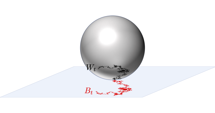
Figure 1: Generating a Brownian motion $\{W_{t}\}_{t\geq 0}$ on a sphere $S^{2}$ by “rolling without slipping” on an Euclidean Brownian motion path $\{B_{t}\}_{t\geq 0}$ in $\mathbb{R}^{2}$.

This allows us to write the Langevin diffusion using the same (formal) notation

$$dZ_{t}=-\operatorname{grad\,}F(Z_{t})\,dt+\sqrt{\frac{2}{\beta}}\,dW_{t}\,,$$ (2.2)

where $\{W_{t}\}_{t\geq 0}$ is a Brownian motion on $M$, and $Z_{0}$ is initialized with a distribution $\mu_{0}$ supported on $M$. We emphasize the above stochastic differential equation (SDE) is interpreted in the sense that for all $f\in C^{2}(M)$, the process $M^{f}(Z)_{t}$ defined in Equation 2.1 is a martingale.

Recall the generator $L\,\phi=\langle-\operatorname{grad\,}F,\operatorname{grad\,}\phi\rangle_{g}+\frac{1}{\beta}\Delta\,\phi$ for all $\phi\in C^{2}(M)$, and the stationary Gibbs density $\nu(x):=\frac{1}{\mathcal{Z}}e^{-\beta F(x)}$ on $M$. We define the carré du champ operator $\Gamma(\phi):=L(\phi^{2})-2\phi\,L\,\phi=\frac{1}{\beta}\,|\operatorname{grad\,}\phi|_{g}^{2}$, and call $(M,\nu,\Gamma)$ the Markov triple as per conventions of [13].

Definition.

We say the Markov triple $(M,\nu,\Gamma)$ satisfies a logarithmic Sobolev inequality with constant $\alpha>0$, denoted $\operatorname{LSI}(\alpha)$, if for all probability measures $\mu$ such that $\mu\ll\nu$ with $h:=\frac{d\mu}{d\nu}\in C^{1}(M)$, we have the inequality

$$H_{\nu}(\mu):=\int_{M}h\log h\,d\nu\leq\frac{1}{2\alpha}\int_{M}\frac{\Gamma(h)}{h}\,d\nu=:\frac{1}{2\alpha}I_{\nu}(\mu)\,,$$ (2.3)

where $H_{\nu}(\mu)$ is the Kullback–Leibler (KL) divergence, and $I_{\nu}(\mu)$ is the relative Fisher information.

Intuitively, Langevin diffusion $Z_{t}$ in Equation 2.2 can be interpreted as a gradient flow in the space of probability distributions [53], and $\operatorname{LSI}(\alpha)$ acts like a gradient domination condition on the KL divergence. Just as Polyak-Łojasiewicz inequality implies an exponential rate of convergence for a gradient flow [77, 58], $\operatorname{LSI}(\alpha)$ implies exponential convergence for Langevin diffusion in this divergence. More precisely, if we let $Z_{t}\sim\rho_{t}$ for all $t\geq 0$, then we have a well known exponential decay result [13, Theorem 5.2.1]

$$H_{\nu}(\rho_{t})\leq H_{\nu}(\rho_{0})\,e^{-2\alpha t}\,.$$ (2.4)

We remark that we chose the Markov triple convention to adjust for a factor of $\beta$. This convention gives us a factor of $e^{-2\alpha t}$ in Equation 2.4, whereas if we choose the LSI convention without reference to the carré du champ operator $\Gamma$, we would end up with a factor of $\exp(-\frac{2\alpha t}{\beta})$ instead. We note there are also alternative approaches to analyze convergence in KL divergence based on a modified LSI [85, 37], which is a strictly weaker condition. While we assume $\operatorname{LSI}(\alpha)$ in this section to establish convergence, we will derive a non-trivial lower bound for $\alpha$ in Section 3.

Assumption 2.2.

$(M,\nu,\Gamma)$ satisfies $\operatorname{LSI}(\alpha)$ for some constant $\alpha>0$. Note our Markov triple convention is temperature dependent, that is for all distribution $\mu$ and $h=\frac{d\mu}{d\nu}$ we have

$$H_{\nu}(\mu)\leq\frac{1}{2\alpha}\frac{1}{\beta}\int\frac{|\operatorname{grad\,}h|_{g}^{2}}{h}\,d\nu\,.$$ (2.5)

We will next turn to discretizing the Langevin diffusion in Equation 2.2. Before we consider the manifold setting, we recall the Langevin algorithm in the Euclidean space $\mathbb{R}^{N}$ with a step size $\eta>0$

$$X_{k+1}=X_{k}-\eta\,\operatorname{grad\,}F(X_{k})+\sqrt{\frac{2\eta}{\beta}}\,\xi_{k}\,\text{ where }\ \xi_{k}\sim N(0,I_{N}).$$ (2.6)

First, we observe that we cannot simply add a gradient update on the manifold, as generally straight lines are not contained on manifolds. Therefore, we propose to instead take a geodesic path starting in the direction of the gradient. This operation is known as the exponential map $\exp:TM\to M$, which is explicitly computable on spheres via the embedding $S^{d}\subset\mathbb{R}^{d+1}$ [4]

$$\exp(x,tv)=x\cos(t|v|)+\frac{v}{|v|}\sin(t|v|)\,,$$ (2.7)

where $x,v\in\mathbb{R}^{d+1}$ such that $|x|=1$, $\langle x,v\rangle=0$, and $t\in\mathbb{R}$. The exponential map can also be naturally extended to the product manifold $M$ by computing it for each sphere separately.

Secondly, we also cannot add an increment of Brownian motion on the manifold, as it is no longer Gaussian. In fact, it is generally difficult to sample Brownian motion increments on manifolds. While the direction is simple (since it is uniform), the magnitude, also known as the radial process, is difficult to sample exactly

$$dr_{t}=\frac{d-1}{2}\cot(r_{t})\,dt+dB_{t}\,.$$ (2.8)

We remark that while an approximation of the diffusion is easy, the analysis of non-exact Brownian increments is difficult to analyze.

This line of work of exact sampling of one dimensional diffusions was first started by [18] based on an idea of rejecting biased samples to recover exact samples. The main breakthrough came with [55], where the authors were able to sample a transformation of the radial process, known as the Wright–Fisher diffusion (see Section D.1). This was further transformed back to an algorithm to sample spherical Brownian motions again by [67]. Since $M$ is a product of spheres, it is equivalent to sampling $n$ independent Brownian increments on $S^{d}$. We provide more details on the sampler in Appendix A.

Putting the two operations together, we can now define the interpolated Langevin update with step size $\eta>0$ as

$$\widehat{X}_{k\eta+t}=\exp(X_{k\eta},-t\operatorname{grad\,}F(X_{k\eta}))\,,\quad X_{k\eta+t}=W\left(\widehat{X}_{k\eta+t},\frac{2t}{\beta}\right)\,,$$ (2.9)

where $W(x,t):M\times\mathbb{R}^{+}\to M$ is a Brownian motion increment starting at $x\in M$ for time $t\geq 0$, and we abuse notation slightly to define the discrete Langevin update as $X_{k}:=X_{k\eta}$ for a step size $\eta>0$. We also initialize $X_{0}\sim\rho_{0}$ where $\rho_{0}$ is supported on $M$.

By viewing one step of the Langevin update as a continuous time process, we can derive a de Bruijn’s identity for the process $\{X_{t}\}_{0\leq t\leq\eta}$.

Lemma 2.3 (De Bruijn’s Identity for the Discretization).

Let $\{X_{t}\}_{0\leq t\leq\eta}$ be the continuous time representation of the Langevin algorithm defined above, and let $\rho_{t}(x)$ be the density of $X_{t}$. Then we have the following de Bruijn type identity

$$\overbrace{\partial_{t}H_{\nu}(\rho_{t})=-I_{\nu}(\rho_{t})}^{\text{de Bruijn's identity}}+\overbrace{\mathbb{E}\left\langle\operatorname{grad\,}F(X_{t})-b(t,X_{0},X_{t})\,,\,\operatorname{grad\,}\log\frac{\rho_{t}(X_{t})}{\nu(X_{t})}\right\rangle_{g}}^{\text{Euclidean discretization error}}$$ (2.10)

$$\qquad\qquad\quad\,\,\underbrace{-\mathbb{E}\operatorname{div}_{X_{t}}b(t,X_{0},X_{t})\log\frac{\rho_{t}(X_{t})}{\nu(X_{t})}}_{\text{Riemannian discretization error}}\,,$$

where we define $\gamma_{t}(x_{0}):=\exp(x_{0},-t\,\operatorname{grad\,}F(x_{0}))$, $b(t,x_{0},x):=P_{\gamma_{t}(x_{0}),x}P_{x_{0},\gamma_{t}(x_{0})}\operatorname{grad\,}F(x_{0})$, and we use $P_{x,y}:T_{x}M\to T_{y}M$ to denote the parallel transport map along the unique shortest geodesic connecting $x,y$ when it exists, and zero otherwise.

The full proof can be found in Section 7.2. Here we observe first component is exactly the classical de Bruijn’s identity $\partial_{t}H_{\nu}(\rho_{t})=-I_{\nu}(\rho_{t})$ for the Langevin diffusion $\{Z_{t}\}_{t\geq 0}$ [13, Proposition 5.2.2]. Since $\operatorname{LSI}(\alpha)$ implies $\partial_{t}H_{\nu}(\rho_{t})=-I_{\nu}(\rho_{t})\leq-2\alpha H_{\nu}(\rho_{t})$, we can almost use a Grönwall type inequality to establish an exponential decay result similar to Equation 2.4. To complete the argument, we seek a bound on the extra terms, which can be interpretted as discretization errors. We note the second term involving the inner product correspond to the error arising from discretizing Langevin diffusion in Euclidean space [87, Equation (31)], hence we call it the Euclidean discretization error. Additionally, the last term is a new source of error arising from the manifold structure.

We emphasize the divergence term in the Riemannian discretization error has the form $\operatorname{div}_{x}P_{y,x}v$ for some $v\in T_{y}M$, and this term diverges as $x$ moves towards the cut locus of $y$, i.e. where the geodesic is no longer unique. Therefore a careful analysis of the distribution of the Brownian motion is required to provide a tight bound on this error term.

We are now ready to state our convergence result for sampling with the Langevin algorithm.

Theorem 2.4 (Sampling Bound in KL Divergence).

Let $F$ satisfy Assumption 2.1, $(M,\nu,\Gamma)$ satisfy Assumption 2.2, and suppose $d\geq 3$. Let $\{X_{k}\}_{k\geq 1}$ be the Langevin algorithm defined in Equation 2.9, with initialization $\rho_{0}\in C^{1}(M)$. If we choose $\beta\geq 1$ and $0\leq\eta\leq\min\left(\frac{2}{3\alpha},\frac{\alpha}{24K_{2}\sqrt{(\beta+d)d}}\right)$, then we have the following bound on the KL divergence of $\rho_{k}:=\mathcal{L}(X_{k})$

$$H_{\nu}(\rho_{k})\leq H_{\nu}(\rho_{0})\,e^{-\alpha k\eta}+45ndK_{2}^{2}\frac{\eta}{\alpha}\,.$$ (2.11)

The full proof can be found in Section 7.5. We reiterate that our convention of $\operatorname{LSI}(\alpha)$ includes an adjustment of a factor of $\beta$ in the Fisher information, more precisely

$$H_{\nu}(\mu)\leq\frac{1}{2\alpha}\frac{1}{\beta}\int\frac{|\operatorname{grad\,}h|_{g}^{2}}{h}\,d\nu\,,$$ (2.12)

where $h=\frac{d\mu}{d\nu}$, and in the case of $\beta=1$ our convention aligns with the usual LSI. We also remark the order matches the best known sampling bound for the Langevin algorithm in an Euclidean space [87]. Given this error bound, we will choose the step size $\eta\leq O\left(\frac{\epsilon\alpha}{ndK_{2}^{2}}\right)$ (note the Theorem also requires $\eta\leq O\left(\frac{1}{\sqrt{\beta}}\right)$), to get the run complexity of $k\geq\Omega\left(\frac{ndK_{2}^{2}}{\alpha^{2}\epsilon}\log\frac{H_{\nu}(\rho_{0})}{\epsilon}\right)$. The dependence on parameters are as follows. We have a linear dependence on dimension $nd$, which is likely tight for the unadjusted Langevin algorithm without additional assumptions, as it matches many existing work with different metrics [87, 20, 29, 31, 33]. In terms of error tolerance, we have $\frac{1}{\epsilon}$, which can only be improved if we use a higher order discretization method or if the target distribution is unbiased (e.g. via Metropolis adjusting). With respect to condition number, we have $\frac{K_{2}^{2}}{\alpha^{2}}=\kappa^{2}$, which matches other existing analysis for KL divergence [87, 20], but it is likely not tight as other analyses of first order methods have achieved better dependence [92]. We will discuss a comparison with other sampling algorithms in Section 5.

2.1 Global Optimization Error

To convert our sampling bound into bounds on optimization error, we now turn our attention to bounding the suboptimality of the Gibbs distribution $\nu$ compared against the global minimum of $F$. We state the following high probability bound.

Theorem 2.5 (Gibbs Suboptimality Bound).

Let $F$ satisfy Assumption 2.1 and suppose $d\geq 3$. For all $\epsilon\in(0,1]$ and $\delta\in(0,1)$, if we choose

$$\beta\geq\frac{3nd}{\epsilon}\log\frac{nK_{2}}{\epsilon\,\delta}\,,$$ (2.13)

then, we have that the Gibbs distribution $\nu(x):=\frac{1}{Z}e^{-\beta F(x)}$ satisfies the following bound

$$\nu\left(F-\min_{y\in M}F(y)\geq\epsilon\right)\leq\delta\,.$$ (2.14)

In other words, samples from $\nu$ find an $\epsilon$-approximate global minimum of $F$ with probability $1-\delta$.

The full proof can be found in Section 8. We observe that dropping logarithmic factors using the notation $\widetilde{\Omega}(\cdot)$, we can write the condition on $\beta$ as $\beta\geq\widetilde{\Omega}(\frac{nd}{\epsilon})$. This dependence is likely tight as it matches the case of quadratic objective functions on $\mathbb{R}^{nd}$, where Gibbs distribution is a Gaussian, and the expected suboptimality is exactly $\frac{nd}{\beta}$. Finally, above results allow us to compute the runtime complexity of the Langevin algorithm to reach an $\epsilon$-global minimum.

Corollary 2.6 (Runtime Complexity).

Let $F$ satisfy Assumption 2.1, and let $(M,\nu,\Gamma)$ satisfy Assumption 2.2. Further let the initialization $\rho_{0}\in C^{1}(M)$, and $d\geq 3$. Then for all choices of $\epsilon\in(0,1]$ and $\delta\in(0,1)$, we can choose

$$\beta \geq\frac{3nd}{\epsilon}\log\frac{2nK_{2}}{\epsilon\,\delta}\,,\quad\eta\leq\min\left\{\frac{2}{3\alpha}\,,\,\frac{\alpha\delta^{2}\sqrt{\epsilon}}{180ndK_{2}^{2}\sqrt{\log\frac{2nK_{2}}{\epsilon\delta}}}\right\}\,,$$ (2.15)

$$k \geq\max\left\{\frac{3}{2}\,,180nd\frac{K_{2}^{2}}{\alpha^{2}}\frac{\sqrt{\log\frac{2nK_{2}}{\epsilon\delta}}}{\delta^{2}\sqrt{\epsilon}}\right\}\left(2\log\frac{2}{\delta}+\log H_{\nu}(\rho_{0})\right)\,,$$

such that the Langevin algorithm $\{X_{k}\}_{k\geq 1}$ defined in Equation 2.9 with distribution $X_{k}\sim\rho_{k}$ satisfies

$$\rho_{k}\left(F-\min_{y\in M}F(y)\geq\epsilon\right)\leq\delta\,.$$ (2.16)

In other words, $X_{k}$ finds an $\epsilon$-global minimum with probability $1-\delta$.

The full proof can be found in Section 10.1. When naively viewing only in terms of the error tolerance $\epsilon>0$, Corollary 2.6 implies that it is sufficient to use $k\geq\widetilde{\Omega}\left(\frac{nd}{\delta^{2}\sqrt{\epsilon}}\right)$ steps to reach an $\epsilon$-global minimum, where $\widetilde{\Omega}(\cdot)$ here hides dependence on other parameters and log factors. However, we note that the logarithmic Sobolev constant $\alpha$ can depend on $\beta$ implicitly, and as $\beta$ depends on $n,d,\epsilon$, this could lead to a worse runtime complexity. In fact, a naive lower bound on $\alpha$ can lead to exponential dependence on these parameters, hence leading to an exponential runtime. We will discuss this in further detail in Section 3, where we establish explicit dependence of $\alpha$ on $n,d,\beta$ that lead to an explicit runtime complexity.

3 LSI and Runtime Complexity

In this section, we provide sufficient conditions for LSI($\alpha$) and a lower bound for the constant $\alpha$. While estimates for LSI constants are well studied [13, 89, 90, 9, 50, 16, 6, 24], we note that straight forward approaches in Euclidean spaces via the Bakry–Émery criterion will not work here, as strong convexity is not possible on compact manifolds. Notably, when there are no spurious local minima, Menz and Schlichting [70] introduced a perturbation method to establish the bound $\alpha^{-1}\leq O(\beta)$, but depends on dimension exponentially. We further improve this result by removing the exponential dependence on dimension $n,d$ in a similar setting.

Assumption 3.1.

$F\in C^{3}(M)$. Without loss of generality, we let $\min_{x\in M}F(x)=0$.

As a consequence of compactness and continuity, there exist constants $K_{1},K_{2},K_{3}\geq 1$ such that $F$ is $K_{1}$-Lipschitz, $\operatorname{grad\,}F$ is $K_{2}$-Lipschitz, and $\nabla^{2}F$ is $K_{3}$-Lipschitz. Here we remark that assuming $F$ is $K_{1}$-Lipschitz does not contradict LSI on a compact manifold.

Assumption 3.2.

The set of global minima $\mathcal{X}:=\{x\in M|F(x)=\inf_{y\in M}F(y)=0\}$ is geodesically convex, i.e. for any two points $x,y\in\mathcal{X}$, the minimum distance geodesic path connecting $x,y$ is also contained in $\mathcal{X}$.

Here we remark this is strictly more general than a unique global minimum.

Assumption 3.3 (Weak Morse).

For all critical points $y$, we have that the Hessian eigenvalues in the escape directions are bounded away from zero. More precisely, there exists $\lambda_{*}\in(0,1]$ such that for all $y$ with $\operatorname{grad\,}F(y)=0$, we have:

1. for all $v\in\operatorname{Ker}(\nabla^{2}F(y)^{\sharp})$, we have that $\operatorname{grad\,}F(\exp_{y}(v))=0$; in other words, $\exp_{y}(v)$ is still a critical point.

2. for all $v\in\operatorname{Ker}(\nabla^{2}F(y)^{\sharp})^{\bot}$, we have that $|\nabla^{2}F(y)^{\sharp}[v]|_{g}\geq\lambda_{*}|v|_{g}$.

Furthermore, for all critical points that is not a global minimum, we have that $\lambda_{\min}(\nabla^{2}F(y))\leq-\lambda_{*}<0$; in other words, there are no spurious local minima, and all saddles points have an escape.

We remark this condition is strictly weaker than a standard Morse assumption (see for example [64]), and we only assume $\lambda_{*}\leq 1$ to simplify computation of explicit constants. Here we note that even if the saddle point has an escape direction, having “flat directions” will also slow down convergence of Langevin diffusion, as it will take longer to “find the saddle point.” This is characterized more precisesly using the Lyapunov functional, and we discuss this further in Section 6.3.2.

We can now state the main result of this section.

Theorem 3.4 (Logarithmic Sobolev Inequality).

Suppose $F$ satisfies Assumption 3.1, 3.3 and 3.2 and $d\geq 2$. Then for all choices of $a,\beta>0$ such that

$$a^{2} \geq\max\left(\frac{24K_{2}nd}{C_{F}^{2}}\,,\frac{160}{\lambda_{*}}\right)\,,\quad\beta\geq a^{2}\max\left(\,\frac{4K_{3}^{2}}{\lambda_{*}^{2}}\,,\,K_{3}^{2}a^{4}\,\right)\,,$$ (3.1)

where $\lambda_{*}$ is defined in Assumption 3.3, we have that the Markov triple $(M,\nu,\Gamma)$ satisfies $\operatorname{LSI}(\alpha)$ with constant

$$\frac{1}{\alpha}=\begin{cases}440\frac{K_{2}n\beta}{\lambda_{*}^{2}}\,,&\text{ if the global minimum is unique, }\\ 605\frac{K_{2}n\beta^{2}}{K_{*}\lambda_{*}}\,,&\text{ otherwise, }\end{cases}$$ (3.2)

where $K_{*}=\exp\left(\frac{-2C_{F}^{2}}{K_{2}K_{3}}\right)$.

The full proof can be found in Section 9. Here, we observe that $\alpha^{-1}\leq O(n\beta)$ or $O(n\beta^{2})$, which is a significant improvement over any standard approach to establishing $\operatorname{LSI}(\alpha)$, where one typically gets exponential dependence on both dimension $nd$ and temperature $\beta$. We also remark that a dimension free Poincaré inequality was established in Proposition 9.14 as an intermediate result; if the global minimum is unique, the constant is also temperature free.

The main bottlenecks preventing improvement at the moment are (1) the requirement that $\beta\gtrsim(nd)^{3}$ for establishing the LSI, which likely can be reduced to $\beta\gtrsim nd$ with a more careful analysis (2) the fact that LSI is worse than Poincaré by a factor of $n\beta$, and we can likely use Poincaré instead to analyze convergence (3) the fact that we did not quotient out the symmetry of the problem, which would yield a unique minimum and improve the dependence on $\beta$ by one order. Putting these together, we would be hopeful of an Poincaré constant of order $\kappa^{-1}=O(1)$ under the requirement of $\beta\gtrsim nd$, which would yield a runtime complexity of $\widetilde{O}(\frac{nd}{\delta^{2}\epsilon^{0.5}})$ from Corollary 2.6. While the runtime complexity can still be improved via a more careful analysis, we note this is first polynomial time result for a Langevin based algorithm, as existing log-Sobolev inequalities on compact manifolds have an exponential dependence on dimension [70].

We will also state the current runtime complexity.

Corollary 3.5.

Let $F:M\to\mathbb{R}$ satisfy Assumption 3.1, 3.2 and 3.3. Let $\{X_{k}\}_{k\geq 1}$ be the Langevin algorithm defined in Equation 2.9, with initialization $\rho_{0}\in C^{1}(M)$, and $d\geq 3$. For all choices of $\epsilon\in(0,1]$ and $\delta\in(0,1)$, if $\beta$ and $\eta$ satisfy the conditions in Corollary 2.6 and Theorem 3.4, then choosing $k$ as

$$k\geq\begin{cases}\widetilde{\Omega}\left(\frac{n^{9.5}d^{8}}{\epsilon^{2.5}\delta^{2}}\right)\,,&\text{ if the global minimum is unique, }\\ \widetilde{\Omega}\left(\frac{n^{15.5}d^{14}}{\epsilon^{4.5}\delta^{2}}\right)\,,&\text{ otherwise, }\end{cases}$$ (3.3)

where $\widetilde{\Omega}(\cdot)$ hides dependence on $\operatorname{poly}\left(K_{2},K_{3},C_{F}^{-1},\lambda_{*}^{-1},K_{*},\log\frac{nd\,K_{2}}{\epsilon\,\delta}\,,\log H_{\nu}(\rho_{0})\,\right)$ and $K_{*}=\exp\left(\frac{-2C_{F}^{2}}{K_{2}K_{3}}\right)$, we have that the Langevin algorithm $\{X_{k}\}_{k\geq 1}$ defined in Equation 2.9 with distribution $\rho_{k}:=\mathcal{L}(X_{k})$ satisfies

$$\rho_{k}\left(F-\min_{y\in M}F(y)\geq\epsilon\right)\leq\delta\,.$$ (3.4)

In other words, $X_{k}$ finds an $\epsilon$-global minimum with probability $1-\delta$.

The proof can be found in Section 10.2. Compared to the exponential runtime of [82] (which considers the Langevin algorithm for non-convex optimization in the Euclidean setting), both of our results are polynomial runtime. This is due to the additional weak Morse and connected minima assumptions in the manifold setting, which yields an LSI constant that has polynomial temperature and dimension dependence, i.e., Theorem 3.4.

4 Application to SDP and Max-Cut

In this section, we discuss an application of the Langevin algorithm for solving the Max-Cut SDP. More specifically, we consider the following SDP for a symmetric matrix $A\in\mathbb{R}^{n\times n}$

$$\operatorname{SDP}(A):= \max_{X}\,\langle A,X\rangle\,,$$ (4.1)

$$\text{subject to }X_{ii}=1\,\text{ for all }\,i\in[n]\,,\text{and }X\succeq 0\,,$$

where $[n]=\{1,2,\cdots,n\}$ and we use $X\succeq 0$ to denote positive semidefiniteness. SDPs have a great number of applications in fields across computer science and engineering. See [35, 66] for a recent survey of methods and applications. In a seminal work, Goemans and Williamson [47] analyzed the SDP in Equation 4.1 as a convex relaxation of the Max-Cut problem on an undirected graph $G$ with adjacency matrix $A_{G}$

$$\operatorname{MaxCut}(A_{G}):=\max_{x_{i}\in\{-1,+1\}}\frac{1}{4}\sum_{i,j=1}^{n}A_{G,ij}(1-x_{i}x_{j})\,,$$ (4.2)

where we the relaxation of the SDP arises from choosing $A=-A_{G}$. Most importantly, the authors introduced a rounding scheme for optimal solutions of the SDP that leads to a $0.878$-optimal Max-Cut. Furthermore, the SDP admits a unique solution under strict complementarity, a condition that is known to be satisfied for almost every cost matrix $A$ (with respect to the Lebesgue on real symmetric matrices) [2]. While it is well known that SDPs can be solved to arbitrary accuracy in polynomial time via interior point methods [72], when used naively, computational costs of these methods scale poorly with the problem dimension $n$. This led to a large literature of fast SDP solvers [1, 3, 83, 43, 59].

In an alternative approach, Burer and Monteiro [15] introduced a low rank and non-convex reparametrization of the convex problem Equation 4.1 given as

$$\operatorname{BM}(A):= \max_{x}\,\langle x,Ax\rangle\,,$$ (4.3)

$$\text{subject to }x=[x^{(1)},\cdots,x^{(n)}]^{\top}\in\mathbb{R}^{n\times(d+1)}\text{ and }|x^{(i)}|=1\text{ for all }i\in[n]\,,$$

where $x^{(i)}\in\mathbb{R}^{d+1}$ and $|x^{(i)}|$ denotes the Euclidean norm. We emphasize this problem is contained in our framework since the manifold is a product of spheres. More precisely, we choose the objective function as

$$F(x):=-\langle x,Ax\rangle+\max_{y\in M}\langle y,Ay\rangle\,,$$ (4.4)

where we observe that the constant offset gives us $\min_{x\in M}F(x)=0$. Furthermore, if we choose $(d+1)(d+2)\geq 2n$, then we also have that the optimal solution to the Burer–Monteiro problem Equation 4.3 is also an optimal solution to the SDP Equation 4.1 [5, 73, 15].

While the Burer–Monteiro problem is non-convex, it is empirically observed that simple first order methods still perform very well [54]. To explain this phenomenon, it was shown that when $(d+1)(d+2)>2n$, all second order stationary points (local minima) are also global minima for almost every cost matrix $A$ [19, 94, 26, 76, 27]. In a different approach by [68], the authors used a Grothendieck-type inequality to show that all critical points are approximately optimal up to a multiplicative factor of $1-\frac{1}{d}$.

Finally, putting these discussion together, we can verify the assumptions required to establish an LSI, and therefore provide a runtime complexity guarantee.

Corollary 4.1.

Let $F$ be the Burer–Monteiro loss function defined in Equation 4.4. Then for all choices of $d$ such that $(d+1)(d+2)>2n$ and almost every cost matrix $A$, $F$ satisfies Assumption 3.1, 3.3 and 3.2.

Furthermore, if we choose $d=\left\lceil\sqrt{2n}\right\rceil$, then for all $\epsilon\in(0,1]$ and $\delta\in(0,1)$, $\beta$ and $\eta$ satisfying the conditions in Corollary 2.6 and Theorem 3.4, and choosing $k$ as

$$k\geq\widetilde{\Omega}\left(\frac{n^{22.5}}{\epsilon^{4.5}\delta^{2}}\right)\,,$$ (4.5)

where $\widetilde{\Omega}(\cdot)$ hides dependence on $\operatorname{poly}\left(K_{2},K_{3},C_{F}^{-1},\lambda_{*}^{-1},K_{*}\log\frac{n\,K_{2}}{\epsilon\,\delta}\,,\log H_{\nu}(\rho_{0})\,\right)$ and $K_{*}=\exp\left(\frac{-2C_{F}^{2}}{K_{2}K_{3}}\right)$, we have that with probability $1-\delta$, the Langevin algorithm $\{X_{k}\}_{k\geq 1}$ defined in Equation 2.9 finds an $\epsilon$-global solution of the SDP Equation 4.1 after $k$ iterations for almost every cost matrix $A$.

Additionally, if we let $\epsilon^{\prime}:=\epsilon/(4\operatorname{MaxCut}(A_{G}))$, then using $X_{k}$ and the random rounding scheme of [47], we recover an $0.878(1-\epsilon^{\prime})$-optimal Max-Cut for almost every adjacency matrix $A_{G}$.

Remark.

Here the notion of almost every cost matrix $A$ is with respect to the Lebesgue measure on real symmetric matrices [2].

As discussed in the earlier section, this is the first polynomial runtime result for the Langevin algorithm; and if the main technical roadblocks of the functional inequalities can be resolved, we are hopeful of a significant improvement in the runtime complexity. For context, we mention some comparable algorithms, including a generic solver of SDP with diagonal constraints $\widetilde{O}(m\epsilon^{-3.5})$ [59], where $m$ is the number of non-sparse entries in the cost matrix $A$; the fast Riemannian trust region method $O(n^{3}d^{2}\epsilon^{-2})$ [68], but each iteration typically cost $O(n^{2}d)$; Block coordinate ascent method $O(n^{3}d^{2}\epsilon^{-2})$ [39] with each iteration typically cost $O(nd)$.

5 Discussion

Extending to general manifolds. Many of the proof techniques used in this paper only depend on knowing an explicit local coordinate system, not the specific manifold structure. However, it is not yet clear which unifying properties are needed to avoid working with known local coordinates. Using comparison theory [57, Section 11] on manifolds with bounded (Ricci and scalar) curvature, we speculate all analyses can be sandwiched by the edge cases: a sphere for maximum curvature and a hyperbolic space for minimum curvature. Therefore, this work can be viewed as the first step in a multiple step program to study Langevin algorithms on general manifolds.

We briefly mention two additional difficulties with extending to more general manifolds. First, we remark Brownian motion increments are difficult to sample on general manifolds. In fact, even sampling on spheres was a recent result [55, 67]. Without a Brownian motion increment, it is difficult to relate the discrete time algorithm Equation 2.9 to the continuous time diffusion Equation 2.2, since the algorithm does not lead to an infinitesimal generator containing the Laplace-Beltrami operator. Second, it is generally difficult to provide a tight bound on the error terms in de Bruijn’s identity without local coordinates. Luckily on spheres, they can be studied via stereographic coordinates (Section C.1) and a transformation to Wright-Fisher diffusion (Section D.1).

Comparison to other samplers. There are known alternative sampling algorithms on manifolds. Most notably, Hamiltonian Monte Carlo (HMC) is widely studied [63, 11, 48, 21, 12]. For optimization, simulated annealing is also often used as a variant of MCMC [56, 14]. From a theoretical perspective, analyzing these algorithms require an orthogonal set of techniques compared to Langevin algorithms. In particular, Metropolis adjusted algorithms are often studied in discrete time in terms of total variation distance [71, 34]. On the other hand, Langevin algorithms are often studied via an approximation by the continuous time Langevin diffusion Equation 2.2, with many techniques rooted in partial differential equations (PDEs) [13]. Therefore, our paper can be seen as complimentary to this line of work, ultimately solving the same problem but with a different set of tools.

Closer to our proposed algorithm, there are variants of projected and proximal Langevin algorithms [8, 10, 92]. While the projected and proximal algorithms have straight forward implementations on the manifold in practice, the analysis of convergence are usually quite difficult. In particular, the main difficulty arises in comparing the randomness of the algorithm to a spherical Brownian motion increment, which is not problematic in Euclidean space as Gaussians are easily sampled and analyzed. As a result, the results of the analyses are not directly comparable. That being said, it is plausible that the analysis of the proximal Langevin algorithm [92] can be extended to our setting, as both our approaches are based on similar techniques from [87]. Several modifications are likely in place to adapt to the manifold setting, for example there will likely be a new Riemannian discretization error term as we had in Lemma 2.3. The proximal algorithm here is particularly interesting as it achieves a higher order bias error term of $O(\eta^{2})$, and therefore yields an improved dependence on the condition number of $\frac{K_{2}^{1.5}}{\alpha^{1.5}}=\kappa^{1.5}$. This suggests that our current result in Theorem 2.4 (which matches [87]) is likely not tight in terms of the condition number. However, the proximal algorithm requires an additional smoothness assumption, results in a higher order dimension dependence, and perhaps most importantly is not directly implementable. Once a proximal solver is introduced, additional error terms will need to be analyzed as well for a fair comparison.

6 Overview of Proofs for Main Theorems

6.1 Convergence of the Langevin Algorithm

In this subsection, we briefly sketch the proof of Theorem 2.4. We first write the one step update as a continuous time process. In particular, we let

$$\widehat{X}_{t}=\exp(X_{0},-t\operatorname{grad\,}F(X_{0}))\,,\quad X_{t}=W\left(\widehat{X}_{t},\frac{2t}{\beta}\right)\,,$$ (6.1)

where recall $\exp:M\times T_{M}\to M$ is the standard exponential map, and $W:M\times\mathbb{R}^{+}\to M$ is an increment of the standard Brownian motion, and further observe that at time $t=\eta$, we have that the discrete time update $X_{1}$ defined in Equation 2.9.

We will attempt to establish a KL divergence bound for this process. For convenience, we will define $\gamma_{t}(x):=\exp(x,-t\operatorname{grad\,}F(x))$, and we will be able to derive a Fokker–Planck equation for $\rho_{t|0}$ which we define as the condition density of $X_{t}$ given $X_{0}=x_{0}$ in Lemma 7.2

$$\partial_{t}\rho_{t|0}(x|x_{0})=\frac{1}{\beta}\Delta\rho_{t|0}(x|x_{0})+\left\langle\operatorname{grad\,}_{x}\rho_{t|0}(x|x_{0}),P_{\gamma_{t}(x_{0}),x}P_{x_{0},\gamma_{t}(x_{0})}\operatorname{grad\,}F(x_{0})\right\rangle_{g}\,,$$ (6.2)

where we add a subscript $x$ to differential operators such as $\operatorname{grad\,}$ to denote the derivative with respect to the $x$ variable as needed, and we use $P_{x,y}:T_{x}M\to T_{y}M$ to denote the parallel transport along the geodesic between $x,y$ when it is unique, and zero otherwise.

Using the Fokker–Planck equation, we can derive a de Bruijn identity for $\rho_{t}$ in Lemma 2.3

$$\partial_{t}H_{\nu}(\rho_{t}) =-I_{\nu}(\rho_{t})+\mathbb{E}\left\langle\operatorname{grad\,}F(X_{t})-b(t,X_{0},X_{t})\,,\,\operatorname{grad\,}\log\frac{\rho_{t}(X_{t})}{\nu(X_{t})}\right\rangle_{g}$$ (6.3)

$$\quad\,\,-\mathbb{E}\operatorname{div}_{X_{t}}b(t,X_{0},X_{t})\log\frac{\rho_{t}(X_{t})}{\nu(X_{t})}\,,$$

where we define $b(t,x_{0},x):=P_{\gamma_{t}(x_{0}),x}P_{x_{0},\gamma_{t}(x_{0})}\operatorname{grad\,}F(x_{0})$.

Here we remark if $X_{t}$ is exactly the Langevin diffusion, then the classical de Bruijn’s identity $\partial_{t}H_{\nu}(\rho_{t})=-I_{\nu}(\rho_{t})$ corresponds to exactly the first term [13, Proposition 5.2.2]. We also observe that the second term involving the inner product correspond to the term arising from discretizing Langevin diffusion in $\mathbb{R}^{nd}$ from [87, Equation 31], hence we call it the Euclidean discretization error. Finally, being on the manifold $M$, we will also get a final term involving $\operatorname{div}_{x}b(t,x_{0},x)$, which requires a careful analysis to give a tight bound.

We will next control the two latter terms. Starting with the inner product term, since it matches the Eucldiean case, we can use the same argument as [87]. In particular, we will need a similar application of Talagrand’s inequality in Lemma 7.4, then via basic Cauchy–Schwarz calculations in Lemma 7.5, we can get

$$\mathbb{E}\left\langle\operatorname{grad\,}F(X_{t})-b(t,X_{0},X_{t})\,,\,\operatorname{grad\,}\log\frac{\rho_{t}(X_{t})}{\nu(X_{t})}\right\rangle_{g}\leq\frac{1}{8}I_{\nu}(\rho_{t})+8tndK_{2}^{2}(1+tK_{2})+\frac{16\beta t^{2}K_{2}^{4}}{\alpha}H_{\nu}(\rho_{0})\,.$$ (6.4)

Now the divergence term from Riemannian discretization error is far more tricky. Using a stereographic local coordinate, we can show a couple of important identities for the divergence of the vector field in Lemma 7.6. Here we use the superscript $(i)$ to denote the $i^{\text{th}}$ sphere component of the product manifold $M$, and use $g^{\prime}$ to denote the Riemannian metric on $S^{d}$. Then we can show

$$\mathbb{E}\left[\left.\operatorname{div}_{X_{t}}b(t,X_{0},X_{t})\right|X_{0}=x_{0}\right] =0\,,$$ (6.5)

$$\mathbb{E}\left[\left.\left(\operatorname{div}_{X_{t}}b(t,X_{0},X_{t})\right)^{2}\right|X_{0}=x_{0}\right] =|\operatorname{grad\,}F(x_{0})|_{g}^{2}\,\left(\frac{2}{d}+1\right)\mathbb{E}\tan\left(\frac{1}{2}d_{g^{\prime}}(\gamma_{t}(x_{0})^{(i)},X_{t}^{(i)})\right)^{2}\,,$$

where $i\in[n]$ is arbitrary.

Observe that $d_{g^{\prime}}(\gamma_{t}(x_{0})^{(\ell)},x^{(\ell)})$ is exactly the geodesic distance traveled by a Brownian motion in time $2t/\beta$. This radial process can be transformed to the well known Wright–Fisher diffusion, which we have a density formula in the form of an infinite series Theorem D.2. Using this formula, we can give an explicit bound on the expected value of the squared divergence term in Lemma 7.7

$$\mathbb{E}\tan\left(\frac{1}{2}d_{g^{\prime}}(\gamma_{t}(x_{0})^{(i)},X_{t}^{(i)})\right)^{2}\leq\frac{4td}{\beta}\,.$$ (6.6)

Here we remark that $\frac{2td}{\beta}$ is the variance of the Brownian motion term in Euclidean space $\mathbb{R}^{d}$, and that $\tan(\theta)\approx\theta$ when $\theta$ is small, therefore this result is tight up to a universal constant.

Returning to the original divergence term in de Bruijn’s identity, we can now split it into two using Young’s inequality. Since the only randomness is a Brownian motion on $M$ when conditioned on $X_{0}$, we can use a local Poincaré inequality with constant $\frac{1}{2t}$, and control the log density ratio term by Fisher information in Proposition 7.9

$$\mathbb{E}\operatorname{div}b(t,X_{0},X_{t})\log\frac{\rho_{t}(X_{t})}{\nu(X_{t})}\leq\frac{1}{8}I_{\nu}(\rho_{t})+\frac{128t^{2}dK_{2}^{2}}{\alpha\beta}H_{\nu}(\rho_{0})+\frac{64t^{2}nd^{2}K_{2}}{\beta^{2}}\,.$$ (6.7)

Putting everything back together into the de Bruijn’s identity, we can get a KL divergence bound using a Grönwall type inequality in Theorem 7.10

$$H_{\nu}(\rho_{t})\leq e^{-\alpha t}H_{\nu}(\rho_{0})+30ndK_{2}^{2}t^{2}\,.$$ (6.8)

The main result Theorem 2.4 follows as a straight forward corollary, where we use a geometric sum bound to to control the KL divergence of $\rho_{k}:=\mathcal{L}(X_{k})$

$$H_{\nu}(\rho_{k})\leq H_{\nu}(\rho_{0})\,e^{-\alpha k\eta}+45ndK_{2}^{2}\frac{\eta}{\alpha}\,.$$ (6.9)

6.2 Suboptimality of the Gibbs Distribution

Recall the Gibbs distribution $\nu=\frac{1}{Z}e^{-\beta F}$, and we want to provide an upper bound on $\nu(F\geq\epsilon)$ given a sufficiently large $\beta>0$. Without loss of generality, we assumed that $\inf_{x}F(x)=0$, and let $x^{*}$ achieve the global min.

The first observation we will make is that $\nu(F\geq\epsilon)$ can be written as a fraction

$$\nu(F\geq\epsilon)=\frac{\int_{F\geq\epsilon}e^{-\beta F}dV_{g}(x)}{\int_{F\geq\epsilon}e^{-\beta F}dV_{g}(x)+\int_{F<\epsilon}e^{-\beta F}dV_{g}(x)}\leq\frac{\int_{F\geq\epsilon}e^{-\beta F}dV_{g}(x)}{\int_{F<\epsilon}e^{-\beta F}dV_{g}(x)}\,.$$ (6.10)

Now observe that the numerator can be upper bounded by

$$\int_{F\geq\epsilon}e^{-\beta F}dV_{g}(x)\leq e^{-\beta\epsilon}\operatorname{Vol}(M)\,,$$ (6.11)

and the denominator can be lower bounded by a quadratic approximation (Lemma 8.1)

$$\int_{F<\epsilon}e^{-\beta F}dV_{g}(x)\geq\int_{B_{R}}e^{-\beta\frac{K_{2}}{2}d_{g}(x,x^{*})^{2}}dV_{g}(x)\,,$$ (6.12)

where $B_{R}:=\{x\in M|\frac{K_{2}}{2}d_{g}(x,x^{*})^{2}<\epsilon\}$, this result follows from $F\leq\frac{K_{2}}{2}d_{g}(x,x^{*})^{2}$ on $B_{R}$.

Next we will use a similar normal coordinates approximation, such that when $R>0$ is sufficiently small, we can approximate the numerator as a Gaussian bound after normalizing the integral (Lemma 8.2 and Equation 8.20)

$$\int_{B_{R}}e^{-\beta\frac{K_{2}}{2}d_{g}(x,x^{*})^{2}}dV_{g}(x)\geq C\beta^{-nd/2}\mathbb{P}[|X|\leq R]\,,$$ (6.13)

where $X\sim N(0,(\beta K_{2})^{-1}I_{nd})$, $C$ is a constant independent of $\beta$ and $\epsilon$. Here $\beta^{-nd/2}$ arises from the normalizing constant of a Gaussian integral. We also observe that we can choose $\beta$ sufficiently large such that $\mathbb{P}[|X|\leq R]\geq 1/2$.

We now return to the original quantity, and observe that it is sufficient to show

$$\nu(F\geq\epsilon)\leq Ce^{-\beta\epsilon}\beta^{nd/2}\leq\delta\,,$$ (6.14)

for some new constant $C$. With some additional calculation, we will see that it is sufficient to choose

$$\beta\geq\frac{C}{\epsilon}\log\frac{1}{\epsilon\delta}\,,$$ (6.15)

which gives us the desired result in Theorem 2.5.

6.3 Logarithmic Sobolev Constant

6.3.1 Existing Results on Lyapunov Conditions

In the context of Markov diffusions, a Lyapunov function is a map $W:M\to[1,\infty)$ that satisfies the following type of condition on a subset $B\subset M$

$$LW\leq-\theta W\,,$$ (6.16)

where $L$ is the Itô generator of the Langevin diffusion in Equation 2.2, and $\theta$ is either a positive constant or a function depending on $x$. Here the set $B$ is chosen usch that the Gibbs measure $\nu$ satisfies a Poincaré inequality when restricted to $M\setminus B$. Under these two conditions, we have that $\nu$ satisfies a Poincaré inequality on $M$ [6, 25]. A slight strengthening of the condition along with a Poincaré inequality also implies a logarithmic Sobolev inequality [24]. The advantage of this approach is that both of these results have made their constants explicit, which allows us to compute explicit dependence on dimension and temperature.

Our work builds on [70], where the authors developed a careful perturbation to remove exponential dependence on $\beta$ due to the Holley–Stroock perturbation. However, after careful calculations, we found this approach still introduced an exponential dependence on dimensions $nd$. To get a polynomial runtime in terms of dimension, we need to develop a new technique without perturbation. We will defer to Section B.4 for more details on the existing Lyapunov methods.

Lyapunov function is often interpreted as an energy quantity that decreases with time, hence controlling a desired process. Alternatively, we can interpret the Lyapunov function as the moment generating function of an escape time, which is well known in the Markov chain literature (see e.g. [34, Theorem 14.1.3]), and first introduced for Markov diffusions in [25, 23]. Let $\{Z_{t}\}_{t\geq 0}$ be the Langevin diffusion defined in Equation 2.2, and we know from the Feynman–Kac formula [7, Theorem 7.15] that the unique solution to $LW=-\theta W$ is

$$W(x)=\mathbb{E}[e^{\theta\tau}|Z_{0}=x]\,,$$ (6.17)

where $\tau:=\{t\geq 0|Z_{t}\notin B\}$ is the first escape time. In fact, the existence of the Feynman–Kac solution is equivalent to the existence of a Lyapunov function [25]. Here we remark that the boundary needs to be handled carefully to an explicit estimate of the Poincaré constant [25].

The proof will come in several steps. First, we will establish an escape time method to finding a Lyapunov function. Secondly, we will prove a Poincaré inequality using the Lyapunov method from [6]. Finally, we will prove the logarithmic Sobolev inequality by adapting HWI inequality approach of [24].

6.3.2 Establishing the Lyapunov Conditions

We will first establish a Lyapunov condition away from all saddle points, i.e. a point $y\in M$ such that $\operatorname{grad\,}F(y)=0$ and the Hessian $\nabla^{2}F(y)$ has at least one negative eigenvalue. Building on [70], we will also choose the Lyapunov function $W(x)=\exp\left(\frac{\beta}{2}F(x)\right)$, and then the Lyapunov condition is reduced to

$$\frac{LW}{W}=\frac{1}{2}\Delta F-\frac{\beta}{4}|\operatorname{grad\,}F|_{g}^{2}\leq-\theta\,.$$ (6.18)

Here we emphasize that Assumption 3.3 is in a sense necessary to upper bound the Lyapunov term by an negative constant, as we require $|\operatorname{grad\,}F|_{g}$ to grow as we move away from the saddle point. This can be interpretted as the “flat directions” of the saddle point can also slow down convergence of Langevin diffusion. We also note this is not unique to Langevin, as even gradient flow alone will yield a similar $-|\operatorname{grad\,}F|_{g}^{2}$ term, and upper bounding this is similar in spirit to the establishing exponential convergence using the Polyak-Łojasiewicz inequality [77, 58].

Therefore choosing a sufficiently large $\beta>0$ will meet the Lyapunov condition (Lemma 9.8). Additionally, we observe that near the unique global minimum, we have either (1) strong convexity of the function $F$, or (2) a positive Ricci curvature on $S^{d}$, hence we get a Poincaré inequality with the classical Bakry–Émery condition. Together this implies a Poincaré inequality away from saddle points (Proposition 9.14).

Next we will choose a second Lyapunov function that satisfies the condition only near saddle points. In particular, we will choose the escape time representation of $W(x)=\mathbb{E}[e^{\theta\tau}|Z_{0}=x]$, where $\tau$ is the first escape time of $Z_{t}$ away from a neighbourhood from each saddle point. Using an equivalent characterization of subexponential random variables (Theorem 9.4), it is equivalent to establish a tail bound of the type

$$\mathbb{P}[\tau>t]\leq c\,e^{-\theta t/2}\,,$$ (6.19)

for some constant $c>0$ and all $t\geq 0$.

To study the escape time, we will first use a “quadratic approximation” of the function $F$ near the saddle point. Then the squared radial process $\frac{1}{2}d_{g}(y,Z_{t})^{2}$ is lower bounded by a Cox–Ingersoll–Ross (CIR) process of the following form

$$d\left[\frac{1}{2}r_{t}^{2}\right]=\left[c_{1}\frac{1}{2}r_{t}^{2}+\frac{c_{2}}{\beta}\right]\,dt+\sqrt{\frac{2}{\beta}}r_{t}\,dB_{t}\,,$$ (6.20)

where $c_{1},c_{2}>0$ are constants specified in the proof.

Since we can compute the density of this process explicitly (Corollary D.6), we can compute a desired escape time bound in Proposition 9.6. Putting it together with the Lyapunov method, we have that $\nu$ satisfies a Poincaré inequality on $M$.

Finally, to get a logarithmic Sobolev inequality, we will use the HWI inequality and Rothaus tightening from [24], which first establishes

$$H_{\nu}(\mu)\leq W_{2}(\mu,\nu)\sqrt{\beta I_{\nu}(\mu)}+\frac{\beta K_{2}}{2}W_{2}(\mu,\nu)^{2}\leq\frac{\tau\beta}{2}I_{\nu}(\mu)+\left(\frac{1}{2\tau}+\frac{\beta K}{2}\right)W_{2}^{2}(\mu,\nu)=:AI_{\nu}(\mu)+B\,,$$ (6.21)

where $\tau>0$ can be optimized later. Then if $\nu$ also satisfies a Poincaré inequality with constant $\kappa$, we can tighten the defective log-Soboelv inequality via Rothaus Lemma to get

$$H_{\nu}(\mu)\leq\left(A+\frac{B+2}{\kappa}\right)I_{\nu}(\mu)\,.$$ (6.22)

The logarithmic Sobolev constant is computed in Theorem 3.4.

7 Convergence of the Langevin Algorithm - Proof of Theorem 2.4

7.1 The Continuous Time Representation

Once again we recall the continuous time process representation of the Langevin algorithm

$$\widehat{X}_{t}=\exp(X_{0},-t\operatorname{grad\,}F(X_{0}))\,,\quad X_{t}=W\left(\widehat{X}_{t},\frac{2t}{\beta}\right)\,,$$ (7.1)

where $\exp:M\times TM\to M$ is the standard exponential map, and $W:M\times\mathbb{R}^{+}\to M$ is a Brownian motion increment. We also recall the notation

$$\gamma_{t}(x):=\exp(x,-t\operatorname{grad\,}F(x))\,.$$ (7.2)

Here we observe that at $t=0$, $\gamma_{0}(x)=x$. At the same time, $X_{t}$ is a Brownian motion starting at $\gamma_{t}(X_{0})$, therefore the (conditional) density of $X_{t}$ starting at $X_{0}=x_{0}$ is

$$\rho_{t|0}(x|x_{0})=p(t,\gamma_{t}(x_{0}),x)\,,$$ (7.3)

where $p(t,y,x)$ is the density of a Brownian motion with diffusion coefficient $\sqrt{2/\beta}$ and starting at $y$. In other words, $p$ is the unique solution to the following heat equation

$$\partial_{t}p(t,y,x)=\frac{1}{\beta}\Delta_{x}p(t,y,x)\,,\quad p(0,y,x)=\delta_{y}(x)\,,\quad x,y\in M\,,$$ (7.4)

where $\Delta_{x}$ denotes the Laplacian (Laplace–Beltrami operator) with respect to the $x$ variable, $\delta_{y}$ is the Dirac delta distribution, and the partial differential equation (PDE) is interpreted in the distributional sense. See [51, Theorem 4.1.1] for additional details on the heat equation and Brownian motion density.

To derive the Fokker–Planck equation, we will need an additional symmetry result about the density $p(t,y,x)$.

Lemma 7.1.

Let $p(t,y,x)$ be the unique solution of Equation 7.4, i.e. the density of a Brownian motion on $M$ with diffusion coefficient $\sqrt{2/\beta}$. For all $x,y\in M$, let $P_{x,y}:T_{x}M\to T_{y}M$ be the parallel transport along the unique shortest geodesic connecting $x,y$ when it exists, and zero otherwise. Then we have

$$\operatorname{grad\,}_{y}p(t,y,x)=-P_{x,y}\operatorname{grad\,}_{x}p(t,y,x)\,,\quad\forall t\geq 0,$$ (7.5)

where we use the subscript $\operatorname{grad\,}_{y}$ to denote the gradient with respect to the $y$ variable.

Proof.

Since $M=S^{d}\times\cdots\times S^{d}$ is a product, it is sufficient to prove the desired result on a single sphere. For the rest of the proof, we will also drop the time variable $t$ and simply write $p(y,x)$ and $p(x,y)$ instead.

We will start by considering the case when there is a unique shortest geodesic connecting $x$ and $y$. Due to Kolmogorov characterization of reversible diffusions [74, Extend Proposition 4.5 to $M$], we have the following identity

$$p(y,x)=p(x,y)\,,\quad\forall\,x,y\in M\,,$$ (7.6)

therefore it is equivalent to prove

$$\operatorname{grad\,}_{y}p(x,y)=-P_{x,y}\operatorname{grad\,}_{x}p(y,x)\,.$$ (7.7)

Let us view $S^{d}$ with center $x$, such that all points $y\in S^{d}$ can be seen as having a radial component $r=d_{g}(x,y)$ and an angular component $\theta\in T_{x}S^{d}$ such that $|\theta|_{g}=1$. Next we observe that since $S^{d}$ is symmetrical in all angular directions, the vector $v=\operatorname{grad\,}_{y}p(x,y)$ must be in the radial direction.

This implies that $r_{t}:=\exp(y,tv)$ is a geodesic, and $r_{\tau}=x$ for some $\tau>0$ (in fact $\tau$ is either $d_{g}(y,x)/|v|_{g}$ or $2\pi-d_{g}(y,x)/|v|_{g}$). Similarly, we can view $S^{d}$ with center $y$, and let $\widetilde{v}=\operatorname{grad\,}_{x}p(y,x)$, such that $\widetilde{r}_{t}:=\exp(x,t\widetilde{v})$ is also a geodesic with $\widetilde{r}_{\tau}=y$. Due to symmetry of $x,y$, we must also have $r_{t}=\widetilde{r}_{\tau-t}$ for all $t\in[0,\tau]$. Since the time derivative of a geodesic is parallel transported along its path, we can write

$$v=\partial_{t}r_{t}|_{t=0}=-\partial_{t}\widetilde{r}_{t}|_{t=\tau}=-P_{\widetilde{r}}\widetilde{v}\,,$$ (7.8)

where we use $P_{\widetilde{r}}$ to denote the parallel transport along the path $\{\widetilde{r}_{t}\}_{t=0}^{\tau}$. To get the desired result, it is sufficient to use the fact that all parallel transports along geodesics to the same end point are equivalent on $S^{d}$, which implies $P_{\widetilde{r}}\widetilde{v}=P_{x,y}\widetilde{v}$.

Finally, we will consider $x,y$ in the cut locus of each other, in other words, $x,y$ are on the opposite poles of $S^{d}$. In this case, we observe that the gradient must remain radial, but symmetrical in all angular directions. Therefore we must have

$$\operatorname{grad\,}_{x}p(y,x)=0\,,$$ (7.9)

which also gives us the desired result.

∎

Lemma 7.2 (Fokker–Planck Equation of the Discretization).

Let $\{X_{t}\}_{t\geq 0}$ be the continuous time representation of the Langevin algorithm defined in Equation 7.1, and let $\rho_{t|0}(x|x_{0})$ be the conditional density of $X_{t}|X_{0}=x_{0}$. Then we have that $\rho_{t|0}$ satisfies the following Fokker–Planck equation

$$\partial_{t}\rho_{t|0}(x|x_{0})=\frac{1}{\beta}\Delta_{x}\rho_{t|0}(x|x_{0})+\left\langle\operatorname{grad\,}_{x}\rho_{t|0}(x|x_{0}),P_{\gamma_{t}(x_{0}),x}P_{x_{0},\gamma_{t}(x_{0})}\operatorname{grad\,}F(x_{0})\right\rangle_{g}\,,$$ (7.10)

where we add a subscript $\operatorname{grad\,}_{x}$ to denote the gradient with respect to the $x$ variable as needed, and we use $P_{x,y}$ to denote the parallel transport along the unique shortest geodesic between $x,y$ when it exists and zero otherwise.

Proof.

We will directly compute the time derivative

$$\partial_{t}\rho_{t|0}(x|x_{0}) =\frac{d}{dt}p(t,\gamma_{t}(x_{0}),x)$$ (7.11)

$$=\partial_{t}p(t,\gamma_{t}(x_{0}),x)+\langle\operatorname{grad\,}_{\gamma_{t}(x_{0})}p(t,\gamma_{t}(x_{0}),x),\partial_{t}\gamma_{t}(x_{0})\rangle_{g}\,,$$

where we use $\frac{d}{dt}$ to denote the time derivative to all variables depending on $t$, and $\partial_{t}$ to denote the derivative with respect to the first variable in $p(t,y,x)$.

Here we observe that

$$\partial_{t}p(t,\gamma_{t}(x_{0}),x)=\frac{1}{\beta}\Delta_{x}p(t,\gamma_{t}(x_{0}),x)\,,$$ (7.12)

due to being the density of the standard Brownian motion.

Next we will observe that since $\gamma_{t}(x_{0})$ is a geodesic, we simply have $\partial_{t}\gamma_{t}(x_{0})=P_{x_{0},\gamma_{t}(x_{0})}(-\operatorname{grad\,}F(x_{0}))$. Furthermore, we can use Lemma 7.1 to write

$$\operatorname{grad\,}_{\gamma_{t}(x_{0})}p(t,\gamma_{t}(x_{0}),x)=-P_{x,\gamma_{t}(x_{0})}\operatorname{grad\,}_{x}p(t,\gamma_{t}(x_{0}),x)\,.$$ (7.13)

Then using the fact that parallel transport preserves the Riemannian inner product, we have that

$$\langle\operatorname{grad\,}_{\gamma_{t}(x_{0})}p(t,\gamma_{t}(x_{0}),x),\partial_{t}\gamma_{t}(x_{0})\rangle_{g}$$ (7.14)

$$=\langle-P_{x,\gamma_{t}(x_{0})}\operatorname{grad\,}_{x}p(t,\gamma_{t}(x_{0}),x),P_{x_{0},\gamma_{t}(x_{0})}(-\operatorname{grad\,}F(x_{0}))\rangle_{g}$$

$$=\langle\operatorname{grad\,}_{x}p(t,\gamma_{t}(x_{0}),x),P_{\gamma_{t}(x_{0}),x}P_{x_{0},\gamma_{t}(x_{0})}\operatorname{grad\,}F(x_{0})\rangle_{g}\,.$$

Finally, rewriting $p(t,\gamma_{t}(x_{0}),x)$ as $\rho_{t|0}(x|x_{0})$ gives us the desired Fokker–Planck equation.

∎

7.2 De Bruijn’s Identity for the Discretization

We will next derive the de Bruijn type identity for the discretization, which we first stated in Lemma 2.3. Here we recall that the Markov triple $(M,\nu,\Gamma)$ is defined as $\nu=\frac{1}{Z}e^{-\beta F}$ and $\Gamma(\phi)=\frac{1}{\beta}|\operatorname{grad\,}\phi|_{g}^{2}$. We will also define $\rho_{t}(x)$ as the density of $X_{t}$, and let $h=\rho_{t}/\nu$. We further recall the KL divergence and Fisher information are defined as

$$H_{\nu}(\rho_{t}) =\int_{M}h\log h\,d\nu=\int_{M}\log\frac{\rho_{t}(x)}{\nu(x)}\,\rho_{t}(x)\,dV_{g}(x)\,,$$ (7.15)

$$I_{\nu}(\rho_{t}) =\int_{M}\frac{\Gamma(h)}{h}\,d\nu=\frac{1}{\beta}\int_{M}\left|\operatorname{grad\,}\log\frac{\rho_{t}(x)}{\nu(x)}\right|_{g}^{2}\,\rho_{t}(x)\,dV_{g}(x)\,,$$

where we recall that $dV_{g}$ is the Riemannian volume form.

Lemma 7.3 (De Bruijn’s Identity for the Discretization).

Let $\{X_{t}\}_{t\geq 0}$ be the continuous time representation of the Langevin algorithm defined in Equation 7.1, and let $\rho_{t}(x)$ be the density of $X_{t}$. Then we have the following de Bruijn type identity

$$\partial_{t}H_{\nu}(\rho_{t})=-I_{\nu}(\rho_{t})+\mathbb{E}\left\langle\operatorname{grad\,}F(X_{t})-b(t,X_{0},X_{t})\,,\,\operatorname{grad\,}\log\frac{\rho_{t}(X_{t})}{\nu(X_{t})}\right\rangle_{g}-\mathbb{E}\operatorname{div}_{X_{t}}b(t,X_{0},X_{t})\log\frac{\rho_{t}(X_{t})}{\nu(X_{t})}\,,$$ (7.16)

where we define

$$b(t,x_{0},x):=P_{\gamma_{t}(x_{0}),x}P_{x_{0},\gamma_{t}(x_{0})}\operatorname{grad\,}F(x_{0})\,,$$ (7.17)

and recall $P_{x,y}:T_{x}M\to T_{y}M$ is the parallel transport map along the unique shortest geodesic connecting $x,y$ when it exists, and zero otherwise.

Proof.

Before we compute the time derivative of KL divergence, we will first compute $\partial_{t}\rho_{t}$ using Lemma 7.2

$$\partial_{t}\rho_{t}(x) =\partial_{t}\int_{M}\rho_{t|0}(x|x_{0})\rho_{0}(x_{0})\,dV_{g}(x_{0})$$ (7.18)

$$=\int_{M}\left[\frac{1}{\beta}\Delta_{x}\rho_{t|0}(x|x_{0})+\left\langle\operatorname{grad\,}_{x}\rho_{t|0}(x|x_{0}),b(t,x_{0},x)\right\rangle_{g}\right]\,\rho_{0}(x_{0})\,dV_{g}(x_{0})$$

$$=\frac{1}{\beta}\Delta_{x}\int_{M}\rho_{t|0}(x|x_{0})\rho_{0}(x_{0})\,dV_{g}(x_{0})+\int_{M}\left\langle\operatorname{grad\,}_{x}\rho_{t|0}(x|x_{0})\rho_{0}(x_{0}),b(t,x_{0},x)\right\rangle_{g}\,dV_{g}(x_{0})$$

$$=\frac{1}{\beta}\Delta_{x}\rho_{t}(x)+\int_{M}\left\langle\operatorname{grad\,}_{x}\rho_{t0}(x,x_{0}),b(t,x_{0},x)\right\rangle_{g}\,dV_{g}(x_{0})\,,$$

where we denote $\rho_{t0}(x,x_{0})$ as the joint density of $(X_{t},X_{0})$.

Returning to the time derivative of KL divergence, we will compute it explicitly using the previous equation

$$\partial_{t}H_{\nu}(\rho_{t}) =\partial_{t}\int_{M}\rho_{t}\log\frac{\rho_{t}}{\nu}\,dV_{g}(x)$$ (7.19)

$$=\int_{M}\partial_{t}\rho_{t}\log\frac{\rho_{t}}{\nu}+\rho_{t}\frac{\partial_{t}\rho_{t}}{\rho_{t}}-\rho_{t}\partial_{t}\log\nu\,dV_{g}(x)$$

$$=\int_{M}\partial_{t}\rho_{t}\log\frac{\rho_{t}}{\nu}\,dV_{g}(x)+\partial_{t}\int_{M}\rho_{t}\,dV_{g}(x)$$

$$=\int_{M}\left[\frac{1}{\beta}\Delta_{x}\rho_{t}(x)+\int_{M}\left\langle\operatorname{grad\,}_{x}\rho_{t0}(x,x_{0}),b(t,x_{0},x)\right\rangle_{g}\,dV_{g}(x_{0})\right]\log\frac{\rho_{t}}{\nu}dV_{g}(x)$$

$$=\int_{M}\frac{1}{\beta}\Delta_{x}\rho_{t}(x)\log\frac{\rho_{t}}{\nu}dV_{g}(x)+\int_{M}\int_{M}\left\langle\operatorname{grad\,}_{x}\rho_{t0}(x,x_{0}),b(t,x_{0},x)\right\rangle_{g}\,dV_{g}(x_{0})\log\frac{\rho_{t}}{\nu}dV_{g}(x)\,.$$

Here we will treat the two integrals separately using integration by parts (divergence theorem). For the first integral, we have that

$$\int_{M}\frac{1}{\beta}\Delta_{x}\rho_{t}(x)\log\frac{\rho_{t}}{\nu}dV_{g}(x)=\int_{M}-\frac{1}{\beta}\left\langle\operatorname{grad\,}\rho_{t}(x),\operatorname{grad\,}\log\frac{\rho_{t}}{\nu}\right\rangle_{g}dV_{g}(x)\,.$$ (7.20)

Next we will use the fact that

$$\rho_{t}(x)\left[\frac{1}{\beta}\operatorname{grad\,}\log\frac{\rho_{t}}{\nu}-\operatorname{grad\,}F(x)\right] =\rho_{t}\left[\frac{1}{\beta}\frac{\operatorname{grad\,}\rho_{t}}{\rho_{t}}-\frac{1}{\beta}\frac{\operatorname{grad\,}\nu}{\nu}-\operatorname{grad\,}F(x)\right]$$ (7.21)

$$=\rho_{t}\left[\frac{1}{\beta}\frac{\operatorname{grad\,}\rho_{t}}{\rho_{t}}+\operatorname{grad\,}F(x)-\operatorname{grad\,}F(x)\right]$$

$$=\frac{1}{\beta}\operatorname{grad\,}\rho_{t}(x)\,,$$

which allows us to write

$$\int_{M}-\frac{1}{\beta}\left\langle\operatorname{grad\,}\rho_{t}(x),\operatorname{grad\,}\log\frac{\rho_{t}}{\nu}\right\rangle_{g}dV_{g}(x) =\int_{M}-\rho_{t}(x)\left\langle\frac{1}{\beta}\operatorname{grad\,}\log\frac{\rho_{t}}{\nu}-\operatorname{grad\,}F(x),\operatorname{grad\,}\log\frac{\rho_{t}}{\nu}\right\rangle_{g}dV_{g}(x)$$ (7.22)

$$=-I_{\nu}(\rho_{t})+\int_{M}\rho_{t}(x)\left\langle\operatorname{grad\,}F(x),\operatorname{grad\,}\log\frac{\rho_{t}}{\nu}\right\rangle_{g}dV_{g}(x)$$

$$=-I_{\nu}(\rho_{t})+\mathbb{E}\left\langle\operatorname{grad\,}F(X_{t}),\operatorname{grad\,}\log\frac{\rho_{t}(X_{t})}{\nu(X_{t})}\right\rangle_{g}\,.$$

For the second integral, we will also use integration by parts to write

$$\int_{M}\int_{M}\left\langle\operatorname{grad\,}_{x}\rho_{t0}(x,x_{0}),b(t,x_{0},x)\right\rangle_{g}\,dV_{g}(x_{0})\log\frac{\rho_{t}}{\nu}dV_{g}(x)$$ (7.23)

$$=-\int_{M}\int_{M}\rho_{t0}(x,x_{0})\operatorname{div}_{x}\left[b(t,x_{0},x)\log\frac{\rho_{t}}{\nu}\right]\,dV_{g}(x_{0})dV_{g}(x)$$

$$=-\int_{M}\int_{M}\rho_{t0}(x,x_{0})\left\langle b(t,x_{0},x),\operatorname{grad\,}\log\frac{\rho_{t}(x)}{\nu(x)}\right\rangle_{g}+\rho_{t0}(x,x_{0})\operatorname{div}_{x}(b(t,x_{0},x))\log\frac{\rho_{t}}{\nu}\,dV_{g}(x_{0})dV_{g}(x)$$

$$=\mathbb{E}\left\langle-b(t,X_{0},X_{t}),\operatorname{grad\,}\log\frac{\rho_{t}(X_{t})}{\nu(X_{t})}\right\rangle_{g}-\mathbb{E}\operatorname{div}_{X_{t}}(b(t,X_{0},X_{t}))\log\frac{\rho_{t}(X_{t})}{\nu(X_{t})}\,.$$

Finally, by merging the two integral terms together, we get the desired identity.

∎

7.3 Bounding the Inner Product Term

Here we will first adapt a Talagrand’s inequality based on the expected gradient from [87, Lemma 11,12].

Lemma 7.4.

Suppose $(M,\nu,\Gamma)$ satisfies $\operatorname{LSI}(\alpha)$ and $\operatorname{grad\,}F$ is $K_{2}$-Lipschitz. Then for all probability distributions $\rho$, we have the bound

$$\int\,|\operatorname{grad\,}F(x)|_{g}^{2}\,d\rho(x)\leq\frac{4K_{2}}{\alpha}H_{\nu}(\rho)+\frac{2ndK_{2}}{\beta}\,.$$ (7.24)

Proof.

Firstly, we observe that by integration by parts

$$\int\Delta F\,d\nu=-\int\langle\operatorname{grad\,}F,\operatorname{grad\,}\nu\rangle_{g}d\operatorname{Vol}=\beta\int\,|\operatorname{grad\,}F|_{g}^{2}d\nu\,.$$ (7.25)

Combined with $K_{2}$-Lipschitzness we get the bound of

$$\int\,|\operatorname{grad\,}F|_{g}^{2}d\nu\leq\frac{ndK_{2}}{\beta}\,.$$ (7.26)

At the same time, recall that we denote $P_{x,y}:T_{x}M\to T_{y}M$ as the parallel transport via the unique shortest geodesic if it exists, we can write

$$|\operatorname{grad\,}F(x)|_{g}\leq|\operatorname{grad\,}F(x)-P_{y,x}\operatorname{grad\,}F(y)|_{g}+|P_{y,x}\operatorname{grad\,}F(y)|_{g}\leq K_{2}d_{g}(x,y)+|\operatorname{grad\,}F(y)|_{g}\,.$$ (7.27)

Now let $\mu(x,y)$ denote the optimal $W_{2}$ coupling of $\rho(x),\nu(y)$, and using $ab\leq\frac{a^{2}}{2}+\frac{b^{2}}{2}$, we can write

$$\int\,|\operatorname{grad\,}F(x)|_{g}^{2}\,d\rho(x) =\int\,|\operatorname{grad\,}F(x)|_{g}^{2}\,d\mu(x,y)$$ (7.28)

$$\leq\int\,\left(K_{2}d_{g}(x,y)+|\operatorname{grad\,}F(y)|_{g}\right)^{2}d\mu(x,y)$$

$$\leq 2K_{2}^{2}W_{2}(\rho,\nu)^{2}+2\int\,|\operatorname{grad\,}F(y)|_{g}^{2}\,d\nu(y)\,,$$

where we used the previous inequality on $|\operatorname{grad\,}F(x)|_{g}$.

Using the fact that $\operatorname{LSI}(\alpha)$ implies the transport inequality $W_{2}(\rho,\nu)^{2}\leq\frac{2}{\alpha}H_{\nu}(\rho)$, and the previous expected gradient bound, we get the desired result

$$2K_{2}^{2}W_{2}(\rho,\nu)^{2}+2\int\,|\operatorname{grad\,}F(y)|_{g}^{2}\,d\nu(y)\leq\frac{4K_{2}^{2}}{\alpha}H_{\nu}(\rho)+\frac{2ndK_{2}}{\beta}\,.$$ (7.29)

∎

Lemma 7.5.

Let $\{X_{t}\}_{t\geq 0}$ be the continuous time representation of the Langevin algorithm defined in Equation 7.1. Suppose further that $(M,\nu,\Gamma)$ satisfies $\operatorname{LSI}(\alpha)$ and $\operatorname{grad\,}F$ is $K_{2}$-Lipschitz, then we have that

$$\mathbb{E}\left\langle\operatorname{grad\,}F(X_{t})-b(t,X_{0},X_{t})\,,\,\operatorname{grad\,}\log\frac{\rho_{t}(X_{t})}{\nu(X_{t})}\right\rangle_{g}\leq\frac{1}{8}I_{\nu}(\rho_{t})+8tndK_{2}^{2}(1+tK_{2})+\frac{16\beta t^{2}K_{2}^{4}}{\alpha}H_{\nu}(\rho_{0})\,,$$ (7.30)

where we define

$$b(t,x_{0},x):=P_{\gamma_{t}(x_{0}),x}P_{x_{0},\gamma_{t}(x_{0})}\operatorname{grad\,}F(x_{0})\,,$$ (7.31)

and recall $P_{x,y}:T_{x}M\to T_{y}M$ is the parallel transport map along the unique shortest geodesic connecting $x,y$ when it exists, and zero otherwise.

Proof.

We start by using the Cauchy-Schwarz and Young’s inequality to write

$$\langle a,b\rangle_{g}\leq|a|_{g}|b|_{g}\leq 2\beta|a|_{g}^{2}+\frac{1}{8\beta}|b|_{g}^{2}\,.$$ (7.32)

Applying this to the inner product term, we can get

$$\mathbb{E}\left\langle\operatorname{grad\,}F(X_{t})-b(t,X_{0},X_{t})\,,\,\operatorname{grad\,}\log\frac{\rho_{t}(X_{t})}{\nu(X_{t})}\right\rangle_{g}\leq 2\beta\,\mathbb{E}\,|\operatorname{grad\,}F(X_{t})-b(t,X_{0},X_{t})|_{g}^{2}\,+\frac{1}{8}I_{\nu}(\rho_{t})\,,$$ (7.33)

therefore, it is sufficient to study the first expectation term.

To this end, we add an intermediate term to the gradient difference

$$\operatorname{grad\,}F(X_{t})-b(t,X_{0},X_{t})$$ (7.34)

$$=\operatorname{grad\,}F(X_{t})-P_{\gamma_{t}(X_{0}),X_{t}}P_{X_{0},\gamma_{t}(X_{0})}\operatorname{grad\,}F(x_{0})$$

$$=\operatorname{grad\,}F(X_{t})-P_{\gamma_{t}(X_{0}),X_{t}}\operatorname{grad\,}F(\gamma_{t}(X_{0}))$$

$$\quad+P_{\gamma_{t}(X_{0}),X_{t}}\operatorname{grad\,}F(\gamma_{t}(X_{0}))-P_{\gamma_{t}(X_{0}),X_{t}}P_{X_{0},\gamma_{t}(X_{0})}\operatorname{grad\,}F(x_{0})\,.$$

Then using triangle inequality and the fact that $\operatorname{grad\,}F$ is $K_{2}$-Lipschitz, we can write

$$|\operatorname{grad\,}F(X_{t})-b(t,X_{0},X_{t})|_{g}$$ (7.35)

$$\leq|\operatorname{grad\,}F(X_{t})-P_{\gamma_{t}(X_{0}),X_{t}}\operatorname{grad\,}F(\gamma_{t}(X_{0}))|_{g}$$

$$\quad+|P_{\gamma_{t}(X_{0}),X_{t}}\operatorname{grad\,}F(\gamma_{t}(X_{0}))-P_{\gamma_{t}(X_{0}),X_{t}}P_{X_{0},\gamma_{t}(X_{0})}\operatorname{grad\,}F(x_{0})|_{g}$$

$$\leq K_{2}d_{g}(\gamma_{t}(X_{0}),X_{t})+K_{2}d_{g}(X_{0},\gamma_{t}(X_{0}))\,,$$

where $d_{g}$ is the geodesic distance.

Now we return to the original expectation term, we can write

$$2\beta\,\mathbb{E}\,|\operatorname{grad\,}F(X_{t})-b(t,X_{0},X_{t})|_{g}^{2} \leq 4\beta K_{2}^{2}\mathbb{E}[d_{g}(\gamma_{t}(X_{0}),X_{t})^{2}+d_{g}(X_{0},\gamma_{t}(X_{0}))^{2}]\,,$$ (7.36)

where we used the inequality $(a+b)^{2}\leq 2a^{2}+2b^{2}$.

Since the process between $\gamma_{t}(X_{0})$ to $X_{t}$ is just a Brownian motion, we can use the radial comparison theorem (Corollary B.6) to write

$$\mathbb{E}d_{g}(\gamma_{t}(X_{0}),X_{t})^{2}\leq\mathbb{E}\frac{2}{\beta}|B_{t}|^{2}=\frac{2tnd}{\beta}\,,$$ (7.37)

where $B_{t}$ is a standard $\mathbb{R}^{nd}$ Brownian motion.

The second term is simply the path between $X_{0}$ and $\gamma_{t}(X_{0})$ is a geodesic, and therefore we have that

$$\mathbb{E}d_{g}(X_{0},\gamma_{t}(X_{0}))^{2}=\mathbb{E}|t\operatorname{grad\,}F(X_{0})|_{g}^{2}\leq t^{2}\left(\frac{4K_{2}^{2}}{\alpha}H_{\nu}(\rho_{0})+\frac{2ndK_{2}}{\beta}\right)\,,$$ (7.38)

where we used the bound from Lemma 7.4.

Putting it together, we can write

$$2\beta\mathbb{E}\,|\operatorname{grad\,}F(X_{t})-b(t,X_{0},X_{t})|_{g}^{2} \leq 4\beta K_{2}^{2}\left[\frac{2tnd}{\beta}+t^{2}\,\left(\frac{4K_{2}^{2}}{\alpha}H_{\nu}(\rho_{0})+\frac{2ndK_{2}}{\beta}\right)\right]$$ (7.39)

$$=8tndK_{2}^{2}(1+tK_{2})+\frac{16\beta t^{2}K_{2}^{4}}{\alpha}H_{\nu}(\rho_{0})\,,$$

which gives us the desired bound.

∎

7.4 Bounding the Divergence Term

Here we define the notation $x=(x^{(1)},\cdots,x^{(n)})\in M$ where $x^{(\ell)}$ represents the coordinate in $\ell^{\text{th}}$ sphere $S^{d}$, and similarly write $v=(v^{(1)},\cdots,v^{(n)})\in T_{x}M$ with $v^{(\ell)}\in T_{x^{(\ell)}}S^{d}$. We will also use $g^{\prime}$ to denote the metric on a single sphere. This allows us to state the a technical result.

Lemma 7.6 (Rotational Symmetry Identity).

Let $\{X_{t}\}_{t\geq 0}$ be the continuous time representation of the Langevin algorithm defined in Equation 7.1. Then we have that

$$\mathbb{E}\left[\left.\operatorname{div}_{X_{t}}b(t,X_{0},X_{t})\right|X_{0}=x_{0}\right] =0\,,$$ (7.40)

$$\mathbb{E}\left[\left.\left(\operatorname{div}_{X_{t}}b(t,X_{0},X_{t})\right)^{2}\right|X_{0}=x_{0}\right] =|\operatorname{grad\,}F(x_{0})|_{g}^{2}\,\left(\frac{2}{d}+1\right)\mathbb{E}\tan\left(\frac{1}{2}d_{g^{\prime}}(\gamma_{t}(x_{0})^{(i)},X_{t}^{(i)})\right)^{2}\,,$$

where $i\in[n]$ is arbitrary.

The full proof can be found in Section C.1 Lemma C.3.

Now we will turn to controlling the quantity in expectation. The next result will use several a couple of well known results regarding the Wright–Fisher diffusion, which we include in Section D.1.

Lemma 7.7.

Let $\{X_{t}\}_{t\geq 0}$ be the continuous time representation of the Langevin algorithm defined in Equation 7.1. For all $t\geq 0$ and $d\geq 3$, we have the following bound

$$\mathbb{E}\tan\left(\frac{1}{2}d_{g^{\prime}}(\gamma_{t}(x_{0})^{(i)},X_{t}^{(i)})\right)^{2}\leq\frac{4td}{\beta}\,.$$ (7.41)

Proof.

We start by invoking Lemma D.1 with the transformation of $Y_{T(t)}=\frac{1}{2}(1-\cos d_{g^{\prime}}(\gamma_{t}(x_{0})^{(i)},X_{t}^{(i)}))$ and the time change $T(t)=2t/\beta$, which implies $Y_{T}$ is a Wright–Fisher diffusion satisfying the SDE

$$dY_{T}=\frac{d}{4}(1-2Y_{T})\,dT+\sqrt{Y_{T}(1-Y_{T})}\,dB_{T}\,,$$ (7.42)

where $\{B_{t}\}_{t\geq 0}$ is a standard Brownian motion in $\mathbb{R}$.

Furthermore, we also have that by the tangent double angle formula, and basic trignometry

$$\tan\left(\frac{1}{2}d_{g^{\prime}}(\gamma_{t}(x_{0})^{(i)},X_{t}^{(i)})\right)^{2} =\tan\left(\frac{1}{2}\arccos(1-2Y_{T})\right)^{2}$$ (7.43)

$$=\frac{1-\cos\circ\arccos(1-2Y_{T})}{1+\cos\circ\arccos(1-2Y_{T})}$$

$$=\frac{Y_{T}}{1-Y_{T}}\,.$$

Using Itô’s Lemma, we have that

$$\frac{Y_{T}}{1-Y_{T}}=\frac{Y_{0}}{1-Y_{0}}+\int_{0}^{T}\,\frac{\frac{d}{4}(1-2Y_{s})+\frac{1}{2}Y_{s}}{(1-Y_{s})^{2}}\,ds+\int_{0}^{T}\,\frac{\sqrt{Y_{s}(1-Y_{s})}}{(1-Y_{s})^{2}}\,dB_{s}\,,$$ (7.44)

and since $Y_{0}=0$ and the Itô integral is a martingale, we can write the desired expectation as

$$\mathbb{E}\tan\left(\frac{1}{2}d_{g^{\prime}}(\gamma_{t}(x_{0})^{(i)},X_{t}^{(i)})\right)^{2}=\mathbb{E}\int_{0}^{T}\,\frac{\frac{d}{4}(1-2Y_{s})+\frac{1}{2}Y_{s}}{(1-Y_{s})^{2}}\,ds\,.$$ (7.45)

We further observe that when $d\geq 3$, we can upper bound the integrand as

$$\frac{\frac{d}{4}(1-2Y_{s})+\frac{1}{2}Y_{s}}{(1-Y_{s})^{2}}=\frac{d-1}{2}\frac{1}{1-Y_{s}}+\frac{2-d}{4}\frac{1}{(1-Y_{s})^{2}}\leq\frac{d-1}{2}\frac{1}{1-Y_{s}}\,,$$ (7.46)

and since the integrand is positive, we can also exchange the order of expectation and integration using Tonelli’s theorem to write

$$\mathbb{E}\tan\left(\frac{1}{2}d_{g^{\prime}}(\gamma_{t}(x_{0})^{(i)},X_{t}^{(i)})\right)^{2}\leq\int_{0}^{T}\,\mathbb{E}\,\frac{d-1}{2}\frac{1}{1-Y_{s}}\,ds\,.$$ (7.47)

At this point we will invoke Theorem D.2 to write the expectation as an integral

$$\mathbb{E}\,\frac{1}{1-Y_{s}}=\int_{0}^{1}\frac{1}{1-y}\sum_{m=0}^{\infty}q_{m}(s)\,\frac{y^{d/2-1}(1-y)^{d/2+m-1}}{B(d/2,d/2+m)}\,dy\,,$$ (7.48)

where $\{q_{m}(s)\}_{m\geq 0}$ is a probability distribution over $\mathbb{N}$ for each $s\geq 0$ and $B(\theta_{1},\theta_{2})$ is the beta function.

Since the integrand is positive, we will once again exchange the order of integration and sum to compute the beta integral

$$\mathbb{E}\,\frac{1}{1-Y_{s}} =\sum_{m=0}^{\infty}q_{m}(s)\,\int_{0}^{1}\,\frac{y^{d/2-1}(1-y)^{d/2+m-2}}{B(d/2,d/2+m)}\,dy$$ (7.49)

$$=\sum_{m=0}^{\infty}q_{m}(s)\,\frac{B(d/2,d/2+m-1)}{B(d/2,d/2+m)}$$

$$=\sum_{m=0}^{\infty}q_{m}(s)\,\frac{d-1}{d/2-1}\,.$$

Using the fact that $d\geq 3$ once again, we have

$$\sum_{m=0}^{\infty}q_{m}(s)\,\frac{d-1}{d/2-1}=\sum_{m=0}^{\infty}q_{m}(s)\frac{2}{1-1/(d-1)}\leq 4\,,$$ (7.50)

which implies

$$\mathbb{E}\tan\left(\frac{1}{2}d_{g^{\prime}}(\gamma_{t}(x_{0})^{(i)},X_{t}^{(i)})\right)^{2}\leq\int_{0}^{2t/\beta}\,2(d-1)\,ds=\frac{4(d-1)t}{\beta}\,,$$ (7.51)

which is the desired result.

∎

Corollary 7.8.

Let $\{X_{t}\}_{t\geq 0}$ be the continuous time representation of the Langevin algorithm defined in Equation 7.1. For all $t\geq 0$ and $d\geq 3$, we have the following bound

$$\mathbb{E}(\operatorname{div}b(t,X_{0},X_{t}))^{2}\leq\frac{8td}{\beta}\mathbb{E}|\operatorname{grad\,}F(X_{0})|_{g}^{2}\,.$$ (7.52)

Proof.

We simply combine the results of Lemmas 7.6 and 7.7 to write

$$\mathbb{E}(\operatorname{div}b(t,x_{0},x))^{2} =\mathbb{E}|\operatorname{grad\,}F(x_{0})|_{g}^{2}\left(\frac{2}{d}+1\right)\mathbb{E}\tan\left(\frac{1}{2}d_{g_{\ell}}(\gamma_{t}(x_{0})_{\ell},x_{\ell})\right)^{2}$$ (7.53)

$$\leq\left(\frac{2}{d}+1\right)\frac{4td}{\beta}\mathbb{E}|\operatorname{grad\,}F(x_{0})|_{g}^{2}\,,$$

and observe that when $d\geq 3$ we have that $2/d+1\leq 2$, which gives us the desired result.

∎

Proposition 7.9.

Let $\{X_{t}\}_{t\geq 0}$ be the continuous time representation of the Langevin algorithm defined in Equation 7.1. Suppose $F$ satisfies Assumption 2.1 and $(M,\nu,\Gamma)$ satisfies Assumption 2.2. Then for all $t\geq 0$ and $d\geq 3$, we have the following bound

$$-\mathbb{E}\operatorname{div}b(t,X_{0},X_{t})\log\frac{\rho_{t}(X_{t})}{\nu(X_{t})}\leq\frac{1}{8}I_{\nu}(\rho_{t})+\frac{128t^{2}dK_{2}^{2}}{\alpha\beta}H_{\nu}(\rho_{0})+\frac{64t^{2}nd^{2}K_{2}}{\beta^{2}}\,.$$ (7.54)

Proof.

We start by observing that

$$\mathbb{E}\log\frac{\rho_{t}(X_{t})}{\nu(X_{t})}=H_{\nu}(\rho_{t})\,,$$ (7.55)

then we can use the fact $\mathbb{E}\operatorname{div}b(t,X_{0},X_{t})=0$ from Lemma 7.6 to write

$$\mathbb{E}\operatorname{div}b(t,X_{0},X_{t})\log\frac{\rho_{t}(X_{t})}{\nu(X_{t})} =\mathbb{E}\operatorname{div}b(t,X_{0},X_{t})\left(\log\frac{\rho_{t}(X_{t})}{\nu(X_{t})}-H_{\nu}(\rho_{t})\right)+H_{\nu}(\rho_{t})\,\mathbb{E}\operatorname{div}b(t,X_{0},X_{t})$$ (7.56)

$$=\mathbb{E}\operatorname{div}b(t,X_{0},X_{t})\left(\log\frac{\rho_{t}(X_{t})}{\nu(X_{t})}-H_{\nu}(\rho_{t})\right)\,.$$

We will then split the first term into two more using Young’s inequality

$$-\mathbb{E}\operatorname{div}b(t,X_{0},X_{t})\left(\log\frac{\rho_{t}(X_{t})}{\nu(X_{t})}-H_{\nu}(\rho_{t})\right)\leq\frac{\epsilon}{2}\mathbb{E}\operatorname{div}b(t,X_{0},X)^{2}+\frac{1}{2\epsilon}\mathbb{E}\left(\log\frac{\rho_{t}(X_{t})}{\nu(X_{t})}-H_{\nu}(\rho_{t})\right)^{2}\,,$$ (7.57)

where $\epsilon>0$ will be chosen later.

Using Corollary 7.8, we can control the first term as

$$\frac{\epsilon}{2}\mathbb{E}\operatorname{div}b(t,X_{0},X)^{2}\leq\frac{\epsilon}{2}\frac{8td}{\beta}\mathbb{E}|\operatorname{grad\,}F(x_{0})|_{g}^{2}\leq\frac{\epsilon}{2}\frac{8td}{\beta}\left(\frac{4K_{2}^{2}}{\alpha}H_{\nu}(\rho_{0})+\frac{2ndK_{2}}{\beta}\right)\,,$$ (7.58)

where we used the bound from Lemma 7.4.

For the second term, we start be rewriting expectation as a double integral over the conditional density first

$$\int_{M}f(x)\,\rho_{t}(x)\,dV_{g}(x)=\int_{M}\int_{M}f(x)\,\rho_{t|0}(x|x_{0})\,dV_{g}(x)\,dV_{g}(x_{0})\,.$$ (7.59)

This way we can use the fact that $\rho_{t|0}(x|x_{0})=p(t,\gamma_{t}(x_{0}),x)$ is the density of a Brownian motion starting at $\gamma_{t}(x_{0})$. Hence using Theorem B.9, $\rho_{t|0}(x|x_{0})$ satisfies a local Poincaré inequality with constant $\frac{1}{2t}$. More precisely, we have that

$$\mathbb{E}\left(\log\frac{\rho_{t}(X_{t})}{\nu(X_{t})}-H_{\nu}(\rho_{t})\right)^{2}\leq\frac{2t}{\beta}\mathbb{E}\left(\operatorname{grad\,}\log\frac{\rho_{t}(X_{t})}{\nu(X_{t})}\right)_{g}^{2}=2t\,I_{\nu}(\rho_{t})\,.$$ (7.60)

To get the desired coefficient on $I_{\nu}(\rho_{t})$, we can simply choose $\epsilon=8t$, and this gives us the bound

$$-\mathbb{E}\operatorname{div}b(t,X_{0},X_{t})\left(\log\frac{\rho_{t}(X_{t})}{\nu(X_{t})}-H_{\nu}(\rho_{t})\right)\leq\frac{32t^{2}d}{\beta}\left(\frac{4K_{2}^{2}}{\alpha}H_{\nu}(\rho_{0})+\frac{2ndK_{2}}{\beta}\right)+\frac{1}{8}I_{\nu}(\rho_{t})\,,$$ (7.61)

which is the desired result.

∎

7.5 Main Result - KL Divergence Bounds

Theorem 7.10 (One Step KL Divergence Bound).

Let $\{X_{t}\}_{t\geq 0}$ be the continuous time representation of the Langevin algorithm defined in Equation 7.1. Assume $F$ satisfies Assumption 2.1 and that $(M,\nu,\Gamma)$ satisfies Assumption 2.2. Then for all $0\leq t\leq\min\left(\frac{2}{3\alpha},\frac{\alpha}{24K_{2}\sqrt{(\beta+d)d}}\right)$ and $d\geq 3$, we have the following growth bound on the KL divergence for $\rho_{t}:=\mathcal{L}(X_{t})$

$$H_{\nu}(\rho_{t})\leq e^{-\alpha t}H_{\nu}(\rho_{0})+30ndK_{2}^{2}t^{2}\,.$$ (7.62)

Proof.

We start by writing down the de Bruijn’s identity for the discretization process from Lemma 2.3

$$\partial_{t}H_{\nu}(\rho_{t})=-I_{\nu}(\rho_{t})+\mathbb{E}\left\langle\operatorname{grad\,}F(X_{t})-b(t,X_{0},X_{t})\,,\,\operatorname{grad\,}\log\frac{\rho_{t}(X_{t})}{\nu(X_{t})}\right\rangle_{g}-\mathbb{E}\operatorname{div}b(t,X_{0},X_{t})\log\frac{\rho_{t}(X_{t})}{\nu(X_{t})}\,.$$ (7.63)

Then using the results Lemma 7.5 and Proposition 7.9, we can get the following bound

$$\partial_{t}H_{\nu}(\rho_{t}) \leq-I_{\nu}(\rho_{t})$$ (7.64)

$$\quad+\frac{1}{8}I_{\nu}(\rho_{t})+16\frac{\beta t^{2}K_{2}^{2}}{\alpha}H_{\nu}(\rho_{0})+8tndK_{2}^{2}(1+tK_{2})$$

$$\quad+\frac{1}{8}I_{\nu}(\rho_{t})+128\frac{t^{2}dK_{2}^{2}}{\alpha\beta}H_{\nu}(\rho_{0})+64\frac{t^{2}nd^{2}K_{2}}{\beta^{2}}\,.$$

Plugging in the Sobolev inequality for $\nu$ and $\beta\geq 1$, we can get

$$\partial_{t}H_{\nu}(\rho_{t}) \leq-\frac{3}{2}\alpha H_{\nu}(\rho_{t})+t(8ndK_{2}^{2})+t^{2}(8K_{2}^{2}+64d)ndK_{2}+t^{2}\frac{K_{2}^{2}}{\alpha}\left(16\beta+128d\right)H_{\nu}(\rho_{0})$$ (7.65)

$$=:-aH_{\nu}(\rho_{t})+c_{1}t+c_{2}t^{2}+c_{3}t^{2}H_{\nu}(\rho_{0})\,.$$

We observe the above is a Grönwall type differential inequality, and using a Grönwall type argument in Lemma E.1, we can get the following bound

$$H_{\nu}(\rho_{t}) \leq e^{-at}H_{\nu}(\rho_{0})+\int_{0}^{t}\,e^{a(s-t)}\,(c_{1}s+c_{2}s^{2}+c_{3}s^{2}H_{\nu}(\rho_{0}))\,ds$$ (7.66)

$$\leq e^{-at}H_{\nu}(\rho_{0})+(c_{1}t+c_{2}t^{2}+c_{3}t^{2}H_{\nu}(\rho_{0}))\int_{0}^{t}\,e^{a(s-t)}\,ds$$

$$=e^{-at}H_{\nu}(\rho_{0})+(c_{1}t+c_{2}t^{2}+c_{3}t^{2}H_{\nu}(\rho_{0}))\frac{1-e^{-at}}{a}$$

$$=e^{-at}\left(1+\frac{e^{at}-1}{a}c_{3}t^{2}\right)H_{\nu}(\rho_{0})+(c_{1}t+c_{2}t^{2})\frac{1-e^{-at}}{a}\,.$$

There are a few simplifications in place. Firstly, we have that $1-e^{-at}\leq at$ for all $t\geq 0$. Then using the fact that $t\leq\frac{2}{3\alpha}=\frac{1}{a}$, we also have that $e^{at}\leq 1+2at$, which gives us

$$H_{\nu}(\rho_{t})\leq e^{-\frac{3}{2}\alpha t}(1+2c_{3}t^{2})H_{\nu}(\rho_{0})+c_{1}t^{2}+c_{2}t^{3}\,.$$ (7.67)

Now we will use the fact that $t\leq\frac{\alpha}{24K_{2}\sqrt{(\beta+d)d}}$ to get that $2c_{3}t^{2}=2\frac{K_{2}^{2}}{\alpha}\left(16\beta+128d\right)t^{2}\leq\frac{1}{2}\alpha t$, which implies the following

$$1+2c_{3}t^{2}\leq 1+\frac{\alpha t}{2}\leq e^{\frac{\alpha}{2}t}\,,$$ (7.68)

and at the same time we also have that

$$c_{2}t^{3}\leq 8ndK_{2}^{2}\left(\frac{K_{2}+64d}{24K_{2}\sqrt{\beta}d}\right)t^{2}\leq 22ndK_{2}^{2}t^{2}\,.$$ (7.69)

Putting these together, we get the desired result of

$$H_{\nu}(\rho_{t})\leq e^{-\alpha t}H_{\nu}(\rho_{0})+30ndK_{2}^{2}t\,.$$ (7.70)

∎

Here we will restate the main result, which was originally Theorem 2.4.

Theorem 7.11 (Finite Iteration KL Divergence Bound).

Let $F$ satisfy Assumption 2.1, $(M,\nu,\Gamma)$ satisfy Assumption 2.2, and suppose $d\geq 3$. Let $\{X_{k}\}_{k\geq 1}$ be the Langevin algorithm defined in Equation 2.9, with initialization $\rho_{0}\in C^{1}(M)$. If we choose $\beta\geq 1$ and $0\leq\eta\leq\min\left(\frac{2}{3\alpha},\frac{\alpha}{24K_{2}\sqrt{(\beta+d)d}}\right)$, then we have the following bound on the KL divergence of $\rho_{k}:=\mathcal{L}(X_{k})$

$$H_{\nu}(\rho_{k})\leq H_{\nu}(\rho_{0})\,e^{-\alpha k\eta}+45ndK_{2}^{2}\frac{\eta}{\alpha}\,.$$ (7.71)

Proof.

From Theorem 7.10, we get that for all positive integers $k$

$$H_{\nu}(\rho_{k})\leq e^{-\alpha\eta}H_{\nu}(\rho_{k-1})+C\eta^{2}\,,$$ (7.72)

where $C=30ndK_{2}^{2}$.

We can then continue to expand the KL divergence term for iteration $k-1$ and smaller to get

$$H_{\nu}(\rho_{k})\leq e^{-\alpha k\eta}H_{\nu}(\rho_{0})+\sum_{\ell=0}^{k-1}e^{-\alpha\ell\eta}C\eta^{2}\,.$$ (7.73)

We can upper bound the second term by an infinite geometric series, hence leading to

$$\sum_{\ell=0}^{k-1}e^{-\alpha\ell\eta}C\eta^{2}\leq C\eta^{2}\frac{1}{1-e^{-\alpha\eta}}\leq C\eta^{2}\frac{1}{\alpha\eta(1-\alpha\eta/2)}\,,$$ (7.74)

where we used the fact that $1-e^{-x}\geq x-x^{2}/2$. Using the constraint that $\eta\leq\frac{2}{3\alpha}$, we further get that

$$\sum_{\ell=0}^{k-1}e^{-\alpha\ell\eta}C\eta^{2}\leq C\frac{3\eta}{2\alpha}\,.$$ (7.75)

Finally, putting everything together, we can get the desired bound for all $k>0$

$$H_{\nu}(\rho_{k})\leq e^{-\alpha k\eta}H_{\nu}(\rho_{0})+45ndK_{2}^{2}\frac{\eta}{\alpha}\,.$$ (7.76)

∎

8 Suboptimality of the Gibbs Distribution - Proof of Theorem 2.5

In this subsection, we attempt to prove results about optimization using the Gibbs distribution

$$\nu(x)=\frac{1}{Z}e^{-\beta F(x)}\,,$$ (8.1)

where $Z$ is the normalizing constant.

Without loss of generality, we shall assume $\min_{x}F(x)=0$, since constant shifts do not affect the algorithm or the distribution. We start with the following approximation Lemma.

Lemma 8.1.

Let $F$ be $K_{2}$-smooth on $(M,g)$, and let $x^{*}$ be any global minimum of $F$. Then for all $\epsilon>0$, we have the following bound

$$\nu(F\geq\epsilon)\leq\frac{e^{-\beta\epsilon}\operatorname{Vol}(M)}{\int_{B_{R}(x^{*})}e^{-\beta\frac{K_{2}}{2}d_{g}(x^{*},x)^{2}}dV_{g}(x)}\,,$$ (8.2)

where $R=\sqrt{2\epsilon/K_{2}}$, $B_{R}(x^{*})$ is the geodesic ball of radius $R$ centered at $x^{*}$, and $d_{g}$ is the geodesic distance.

Proof.

We start by defining the unnormalized measure

$$\widehat{\nu}_{F}(A):=\int_{A}e^{-\beta F(x)}dV_{g}(x)\,.$$ (8.3)

Then letting $D_{\epsilon}(F):=\{x:F(x)<\epsilon\}$, we can rewrite the desired probability as

$$\nu(F\geq\epsilon)=\frac{\widehat{\nu}_{F}(D_{\epsilon}(F)^{c})}{\widehat{\nu}_{F}(D_{\epsilon}(F))+\widehat{\nu}_{F}(D_{\epsilon}(F)^{c})}\,.$$ (8.4)

Observe that right hand side is now a function of $F$, and to achieve an upper bound, it is sufficient to modify $F$ such that either increase $\widehat{\nu}_{F}(D_{\epsilon}(F)^{c})$ and/or decrease $\widehat{\nu}_{F}(D_{\epsilon}(F))$.

More precisely, for any function $G$ such that

$$\widehat{\nu}_{F}(D_{\epsilon}(F))\geq\widehat{\nu}_{G}(D_{\epsilon}(G))\,,\quad\widehat{\nu}_{F}(D_{\epsilon}(F)^{c})\leq\widehat{\nu}_{G}(D_{\epsilon}(G)^{c})\,,$$ (8.5)

we then also have

$$\frac{\widehat{\nu}_{F}(D_{\epsilon}(F)^{c})}{\widehat{\nu}_{F}(D_{\epsilon}(F))+\widehat{\nu}_{F}(D_{\epsilon}(F)^{c})}\leq\frac{\widehat{\nu}_{G}(D_{\epsilon}(G)^{c})}{\widehat{\nu}_{G}(D_{\epsilon}(G))+\widehat{\nu}_{G}(D_{\epsilon}(G)^{c})}\,.$$ (8.6)

To this goal, we will upper bound $F$ near $x^{*}$ using a “quadratic” function, i.e.

$$G(x)=\frac{K_{2}}{2}d_{g}(x^{*},x)\,,\quad x\in B_{R}(x^{*})^{2}\,.$$ (8.7)

To see that $G(x)\geq F(x)$ on $B_{R}(x^{*})$, we will let $\gamma(t)$ be the unit speed geodesic such that $\gamma(0)=x^{*}$ and $\gamma(d_{g}(x^{*},x))=x$. Then using the fact that $F(x^{*})=0$ and $dF(x^{*})=0$, we can write

$$F(x)=\int_{0}^{d_{g}(x^{*},x)}dF(\dot{\gamma}(s_{1}))\,ds_{1}=\int_{0}^{d_{g}(x^{*},x)}\int_{0}^{s_{1}}\nabla^{2}F(\dot{\gamma}(s_{2}),\dot{\gamma}(s_{2}))ds_{2}\,ds_{1}\,.$$ (8.8)

Using the fact that $F$ is $K_{2}$-smooth and $\gamma(t)$ is unit speed, we can upper bound the integrand by $K_{2}$, and therefore we can write

$$\int_{0}^{d_{g}(x^{*},x)}\int_{0}^{s_{1}}\nabla^{2}F(\dot{\gamma}(s_{2}),\dot{\gamma}(s_{2}))ds_{2}\,ds_{1}\leq\int_{0}^{d_{g}(x^{*},x)}\int_{0}^{s_{1}}K_{2}ds_{2}\,ds_{1}=\frac{K_{2}}{2}d_{g}(x^{*},x)^{2}\,,$$ (8.9)

which is the desired bound.

For $x\notin B_{R}(x^{*})$, we will simply define $G(x):=\epsilon$. Then we must have that

$$\widehat{\nu}_{F}(D_{\epsilon}(F))=\int_{D_{\epsilon}(F)}e^{-\beta F(x)}dV_{g}(x)\geq\int_{D_{\epsilon}(G)}e^{-\beta G(x)}dV_{g}(x)=\widehat{\nu}_{G}(D_{\epsilon}(G))\,,$$ (8.10)

since $D_{\epsilon}(G)\subset D_{\epsilon}(F)$ and $e^{-\beta F}\geq e^{-\beta G}$.

The other direction is obtained similarly

$$\widehat{\nu}_{F}(D_{\epsilon}(F)^{c})=\int_{D_{\epsilon}(F)^{c}}e^{-\beta F(x)}dV_{g}(x)\leq\int_{D_{\epsilon}(F)^{c}}e^{-\beta\epsilon}dV_{g}(x)\leq\int_{D_{\epsilon}(G)^{c}}e^{-\beta\epsilon}dV_{g}(x)=\widehat{\nu}_{G}(D_{\epsilon}(G)^{c})\,.$$ (8.11)

Putting everything together, we get

$$\frac{\widehat{\nu}_{F}(D_{\epsilon}(F)^{c})}{\widehat{\nu}_{F}(D_{\epsilon}(F))+\widehat{\nu}_{F}(D_{\epsilon}(F)^{c})} \leq\frac{\widehat{\nu}_{G}(D_{\epsilon}(G)^{c})}{\widehat{\nu}_{G}(D_{\epsilon}(G))+\widehat{\nu}_{G}(D_{\epsilon}(G)^{c})}$$ (8.12)

$$=\frac{e^{-\beta\epsilon}\operatorname{Vol}(M\setminus B_{R}(x^{*}))}{e^{-\beta\epsilon}\operatorname{Vol}(M\setminus B_{R}(x^{*}))+\int_{B_{R}(x^{*})}e^{-\beta\frac{K_{2}}{2}d_{g}(x^{*},x)^{2}}dV_{g}(x)}\,.$$

We get the desired result by further upper bounding this term by

$$\frac{e^{-\beta\epsilon}\operatorname{Vol}(M\setminus B_{R}(x^{*}))}{e^{-\beta\epsilon}\operatorname{Vol}(M\setminus B_{R}(x^{*}))+\int_{B_{R}(x^{*})}e^{-\beta\frac{K_{2}}{2}d_{g}(x^{*},x)^{2}}dV_{g}(x)}\leq\frac{e^{-\beta\epsilon}\operatorname{Vol}(M)}{\int_{B_{R}(x^{*})}e^{-\beta\frac{K_{2}}{2}d_{g}(x^{*},x)^{2}}dV_{g}(x)}\,.$$ (8.13)

∎

Lemma 8.2.

For $R\leq\pi/2$ and $\beta\geq\frac{nd}{R^{2}K_{2}}$, we have the following lower bound

$$\int_{B_{R}(x^{*})}e^{-\beta\frac{K_{2}}{2}d_{g}(x^{*},x)^{2}}dV_{g}(x)\geq\left(\frac{2}{\pi}\right)^{n(d-1)}\left(\frac{2\pi}{\beta K_{2}}\right)^{nd/2}\left[1-\exp\left(-\frac{1}{2}(R^{2}\beta K_{2}/2-nd)\right)\right]\,.$$ (8.14)

Proof.

We begin by rewriting the integral in normal coordinates, and observe that a geodesic ball $B_{R}(x^{*})\subset M$ is then $B_{R}(0)\subset\mathbb{R}^{nd}$. Then we get

$$\int_{B_{R}(x^{*})}e^{-\beta\frac{K_{2}}{2}d_{g}(x^{*},x)^{2}}dV_{g}(x)=\int_{B_{R}(0)}e^{-\beta\frac{K_{2}}{2}|x|^{2}}\sqrt{\det g}\,dx\,,$$ (8.15)

where $g$ is the Riemannian metric on $M=S^{d}\times\cdots S^{d}$ ($n$-times).

At this point, we observe the block diagonal structure of $g$ gives us

$$\det g=(\det g_{S^{d}})^{n}\,,$$ (8.16)

where $g_{S^{d}}$ is the Riemannian metric of $S^{d}$ in normal coordinates. Finally, we can also have the lower bound from Lemma C.5 whenever $|y|\leq\pi/2$

$$\det g_{S^{d}}\geq\left(\frac{2}{\pi}\right)^{2(d-1)}\,.$$ (8.17)

This then implies the lower bound on the volume form

$$\sqrt{\det g}\geq\left(\frac{2}{\pi}\right)^{n(d-1)}\,,$$ (8.18)

leading to the following integral lower bound

$$\int_{B_{R}(x^{*})}e^{-\beta\frac{K_{2}}{2}d_{g}(x^{*},x)^{2}}dV_{g}(x)\geq\left(\frac{2}{\pi}\right)^{n(d-1)}\int_{B_{R}(0)}e^{-\beta\frac{K_{2}}{2}|x|^{2}}dx\,.$$ (8.19)

We next observe the above integral is an unnormalized Gaussian integral in $\mathbb{R}^{nd}$ with variance $(\beta K_{2})^{-1}$. So we can rewrite the integral as

$$\int_{B_{R}(0)}e^{-\beta\frac{K_{2}}{2}|x|^{2}}dx=\left(\frac{2\pi}{\beta K_{2}}\right)^{nd/2}\mathbb{P}[|Z|\leq R\sqrt{\beta K_{2}}]\,,$$ (8.20)

where $Z\sim N(0,I_{nd})$ is a standard Gaussian.

At this point, it is sufficient to provide a Gaussian tail bound, since

$$\mathbb{P}[|Z|\leq R\sqrt{\beta K_{2}}]=1-\mathbb{P}[|Z|\geq R\sqrt{\beta K_{2}}]=1-\mathbb{P}[|Z|-\mathbb{E}|Z|\geq R\sqrt{\beta K_{2}}-\mathbb{E}|Z|]\,.$$ (8.21)

Using the Cauchy-Schwarz inequality, we get that

$$\mathbb{E}|Z|\leq\sqrt{\mathbb{E}|Z|^{2}}=\sqrt{nd}\,,$$ (8.22)

and therefore we can bound

$$\mathbb{P}[|Z|-\mathbb{E}|Z|\geq R\sqrt{\beta K_{2}}-\mathbb{E}|Z|]\leq\mathbb{P}[|Z|-\mathbb{E}|Z|\geq R\sqrt{\beta K_{2}}-\sqrt{nd}]\,.$$ (8.23)

Using the assumption $\beta\geq\frac{nd}{R^{2}K_{2}}$, we ensure that $R\sqrt{\beta K_{2}}-\sqrt{nd}\geq 0$, hence we can use the $1$-Lipschitz concentration bound to get

$$\mathbb{P}[|Z|-\mathbb{E}|Z|\geq R\sqrt{\beta K_{2}}-\sqrt{nd}]\leq\exp\left(-\frac{1}{2}\left(R\sqrt{\beta K_{2}}-\sqrt{nd}\right)^{2}\right)\,.$$ (8.24)

Here we will use Young’s inequality to write $ab\leq\frac{a^{2}}{4}+b^{2}$, which leads to

$$(a-b)^{2}=a^{2}+b^{2}-2ab\geq a^{2}+b^{2}-\frac{1}{2}a^{2}-2b^{2}=\frac{1}{2}a^{2}-b^{2}\,,$$ (8.25)

and applying to $a=R\sqrt{\beta K_{2}},b=\sqrt{nd}$, we get that

$$\exp\left(-\frac{1}{2}\left(R\sqrt{\beta K_{2}}-\sqrt{nd}\right)^{2}\right)\leq\exp\left(-\frac{1}{2}\left(R^{2}\beta K_{2}/2-nd\right)\right)\,.$$ (8.26)

Putting everything together, we get the desired lower bound

$$\int_{B_{R}(x^{*})}e^{-\beta\frac{K_{2}}{2}d_{g}(x^{*},x)^{2}}dV_{g}(x)\geq\left(\frac{2}{\pi}\right)^{n(d-1)}\left(\frac{2\pi}{\beta K_{2}}\right)^{nd/2}\left[1-\exp\left(-\frac{1}{2}(R^{2}\beta K_{2}/2-nd)\right)\right]\,.$$ (8.27)

∎

We will now restate our main result on suboptimality, originally Theorem 2.5.

Theorem 8.3 (Gibbs Suboptimality Bound).

Let $F$ satisfy Assumption 2.1 and suppose $d\geq 3$. Then for all $\epsilon\in(0,1]$ and $\delta\in(0,1)$, when we choose

$$\beta\geq\frac{3nd}{\epsilon}\log\frac{nK_{2}}{\epsilon\,\delta}\,,$$ (8.28)

then we have that the Gibbs distribution $\nu(x):=\frac{1}{Z}e^{-\beta F(x)}$ satisfies the following bound

$$\nu\left(F-\min_{y\in M}F(y)\geq\epsilon\right)\leq\delta\,.$$ (8.29)

In other words, $\nu$ finds an $\epsilon$-approximate global minimum of $F$ with probability $1-\delta$.

Proof.

Given the results of Lemma 8.1 and Lemma 8.2, we have the following upper bound by choosing $R=\sqrt{2\epsilon/K_{2}}$

$$\nu(F\geq\epsilon)\leq\frac{e^{-\beta\epsilon}\operatorname{Vol}(M)}{\left(\frac{2}{\pi}\right)^{n(d-1)}\left(\frac{2\pi}{\beta K_{2}}\right)^{nd/2}\left[1-\exp\left(-\frac{1}{2}(\epsilon\beta-nd)\right)\right]}\,,$$ (8.30)

when $0<\epsilon\leq 1\leq\frac{\pi^{2}K_{2}}{8}$, and $\beta\geq\frac{nd}{2\epsilon}$, which is satisfied when $\beta\geq\frac{1}{\epsilon}(nd+2\log 2)$.

Therefore it is sufficient to compute a lower bound condition on $\beta$ such that the right hand side term is less than $\delta$. To this end, we start by computing the requirement for $\beta$ such that

$$1-\exp\left(-\frac{1}{2}(\epsilon\beta-nd)\right)\geq\frac{1}{2}\,.$$ (8.31)

Rearranging and taking $log$ of both sides, it is equivalent to satisfy the condition

$$\frac{nd}{2}-\frac{\beta\epsilon}{2}\leq-\log 2\,,$$ (8.32)

hence it is sufficient to have $\beta\geq\frac{1}{\epsilon}(nd+2\log 2)$.

Therefore we have the upper bound

$$\nu(F\geq\epsilon)\leq e^{-\beta\epsilon}\beta^{nd/2}\frac{\operatorname{Vol}(M)}{\left(\frac{2}{\pi}\right)^{n(d-1)}\left(\frac{2\pi}{K_{2}}\right)^{nd/2}\frac{1}{2}}\,.$$ (8.33)

For now, let us define

$$C:=\frac{\operatorname{Vol}(M)}{\left(\frac{2}{\pi}\right)^{n(d-1)}\left(\frac{2\pi}{K_{2}}\right)^{nd/2}\frac{1}{2}}\,,$$ (8.34)

then to get the desired result, it is sufficient to show

$$e^{-\beta\epsilon}\beta^{nd/2}C\leq\delta\,.$$ (8.35)

Taking $log$ and rearranging, we have the equivalent condition of

$$\beta\epsilon-\frac{nd}{2}\log\beta\geq\log C+\log\frac{1}{\delta}\,.$$ (8.36)

Here we will first observe that $\frac{\beta\epsilon}{2}-\frac{nd}{2}\log\beta$ will be an increasing function in terms of $\beta$ after a local minimum, therefore we compute this local minimum by differentiating with respect to $\beta$ to get

$$0=\frac{\epsilon}{2}-\frac{nd}{2\beta}\,,$$ (8.37)

therefore we have the local minimum is at $\beta=\frac{nd}{\epsilon}$, and therefore for all $\beta\geq\frac{nd}{\epsilon}$, we have that

$$\frac{\beta\epsilon}{2}-\frac{nd}{2}\log\beta\geq\frac{nd}{2}\left(1-\log\frac{nd}{\epsilon}\right)\,.$$ (8.38)

Since we already require $\beta\geq\frac{1}{\epsilon}(nd+2\log 2)$, we have it is sufficient to show

$$\frac{\beta\epsilon}{2}+\frac{nd}{2}\left(1-\log\frac{nd}{\epsilon}\right)\geq\log C+\log\frac{1}{\delta}\,,$$ (8.39)

and we rearrange to get

$$\beta\geq\frac{1}{\epsilon}\left[2\log C+2\log\frac{1}{\delta}+nd\left(\log\frac{nd}{\epsilon}-1\right)\right]\,.$$ (8.40)

Therefore it simply remains to compute an upper bound for $\log C$. We start by writing out the exact term

$$\log C=\log\operatorname{Vol}(M)+n(d-1)\log\frac{\pi}{2}+\frac{nd}{2}\log\frac{K_{2}}{2\pi}+\log 2\,.$$ (8.41)

We will group the $nd$ terms by upper bounding

$$n(d-1)\log\frac{\pi}{2}+\frac{nd}{2}\log\frac{K_{2}}{2\pi}\leq nd\log\frac{\pi}{2}\sqrt{\frac{K_{2}}{2\pi}}=nd\log\sqrt{\frac{\pi K_{2}}{8}}\leq\frac{nd}{2}\log\frac{K_{2}}{2}\,,$$ (8.42)

where we used the fact that $\frac{\pi}{8}<\frac{1}{2}$.

Then we observe that

$$\log\operatorname{Vol}(M)=n\log\operatorname{Vol}(S^{d})=n\log\frac{(d+1)\pi^{(d+1)/2}}{\Gamma(\frac{d+1}{2}+1)}\,.$$ (8.43)

Now we will use a Stirling’s approximation bound from Lemma E.2 to write

$$\Gamma\left(\frac{d+1}{2}+1\right)\geq\sqrt{2\pi}\left(\frac{d+1}{2}\right)^{d/2+1}e^{-(d+1)/2}\,,$$ (8.44)

which gives us the bound on volume

$$\log\operatorname{Vol}(M)\leq n\log\left[(e\pi)^{(d+1)/2}\left(\frac{d+1}{2}\right)^{-d/2}\sqrt{\frac{2}{\pi}}\right]=n\left[\frac{-d}{2}\left(\log\frac{d+1}{2}-1-\log\pi\right)+\frac{1}{2}(1+\log 2)\right]\,.$$ (8.45)

Since we have $d\geq 3$, we group the constant in for simplicity by bounding

$$\frac{1}{2}(1+\log 2)\leq\frac{d}{6}(1+\log 2)\,,$$ (8.46)

which gives us a cleaner form

$$\log\operatorname{Vol}(M)\leq nd\left[\frac{-1}{2}\log\frac{d+1}{2}+\frac{1+\log\pi}{2}+\frac{1}{6}(1+\log 2)\right]\leq nd\left[\frac{-1}{2}\log\frac{d+1}{2}+2\right]\,,$$ (8.47)

where we used the fact that $\frac{1+\log\pi}{2}+\frac{1}{6}(1+\log 2)\approx 1.35<2$.

Putting the $\log C$ terms together, we get the bound

$$\log C\leq nd\left(\frac{1}{2}\log\frac{K_{2}}{2}-\frac{1}{2}\log\frac{d+1}{2}+2\right)+\log 2\,,$$ (8.48)

and putting the above expression back to the lower bound on $\beta$, we get

$$\frac{1}{\epsilon}\left[2nd\left(\frac{1}{2}\log\frac{K_{2}}{2}-\frac{1}{2}\log\frac{d+1}{2}+2\right)+2\log 2+2\log\frac{1}{\delta}+nd\left(\log\frac{nd}{\epsilon}-1\right)\right]$$ (8.49)

$$=\frac{1}{\epsilon}\left[nd\left(\log\frac{2nd}{\epsilon(d+1)}+\log\frac{K_{2}}{2}+3\right)+2\log\frac{1}{\delta}+2\log 2\right]$$

$$\leq\frac{1}{\epsilon}\left[nd\left(\log\frac{2n}{\epsilon}+\log\frac{K_{2}}{2}+3\right)+2\log\frac{1}{\delta}+2\log 2\right]\,.$$

To get the desired sufficient lower bound for $\beta$, we clean up the constants using the fact that $K_{2}\geq 1$, $\log 2<0$ to get

$$\beta\geq\frac{3nd}{\epsilon}\log\frac{nK_{2}}{\epsilon\,\delta}\,.$$ (8.50)

∎

9 Escape Time Approach to Lyapunov - Proof of Theorem 3.4

9.1 Equivalent Escape Time Formulation

In this section, we will study a construction of Lyapunov function using escape time. In particular, we consider a partition of $M=B\sqcup B^{c}$, such that $B$ is open, $\partial B\in C^{1}(M)$, and $\nu$ satisfies a Poincaré inequality when restricted to $B^{c}$. With this in mind, we will introduce the following definition.

Definition 9.1.

$W\in C^{2}(M)$ is said to be a Lyapunov function on $B\subset M$ with parameters $\theta>0,b\geq 0$ if $W\geq 1$ and

$$LW\leq-\theta W\,,\quad x\in B\,.$$ (9.1)

Recall Theorem B.12 adapted from [6], if $W$ is a Lyapunov function under the above conditions, then $\nu$ satisfies a Poincaré inequality on $M$. For the rest of this section, we will construct a Lyapunov function $W$ in terms of an escape time of $Z_{t}$.

To start, we recall the Langevin diffusion on $M$

$$dZ_{t}=-\operatorname{grad\,}F(Z_{t})\,dt+\sqrt{\frac{2}{\beta}}\,dW_{t}\,,$$ (9.2)

and it has the generator

$$L\phi=\langle-\operatorname{grad\,}\phi,\operatorname{grad\,}F\rangle_{g}+\frac{1}{\beta}\Delta\phi\,,\quad\forall\phi\in C^{2}(M)\,.$$ (9.3)

With this in mind, we define the first escape time outside of $B$

$$\tau_{B^{c}}:=\inf\{t\geq 0|Z_{t}\notin B\}\,,$$ (9.4)

and we also define $\mathbb{E}_{x}[\,\cdots\,]:=\mathbb{E}[\,\cdots\,|Z_{0}=x]$.

Then we will recall the classic Feynman–Kac theorem for the bounded domain.

Theorem 9.2.

[7, Theorem 7.15] Suppose $u$ is a unique solution to the following Dirichlet problem

$$\begin{cases}-Lu+k(x)u=h(x)\,,&x\in B\,,\\ u(x)=\overline{h}(x)\,,&x\in\partial B\,,\end{cases}$$ (9.5)

and further assume

$$\mathbb{E}_{x}\left[\tau_{B^{c}}\exp\left(\inf_{x\in B}k(x)\tau_{B^{c}}\right)\right]<\infty\,,\quad x\in B\,.$$ (9.6)

Then we have the following stochastic representation

$$u(x) =\mathbb{E}_{x}\bigg{[}\overline{h}(Z_{\tau_{B^{c}}})\exp\left(-\int_{0}^{\tau_{B^{c}}}k(Z_{s})\,ds\right)+\int_{0}^{\tau_{B^{c}}}h(Z_{\tau_{B^{c}}})\exp\left(-\int_{0}^{t}k(Z_{s})\,ds\right)\,dt\bigg{]}\,,\quad\forall x\in B\,.$$ (9.7)

As a consequence, if $\tau_{B^{c}}$ is exponentially integrable, then we have an explicit formula for a Lyapunov function.

Corollary 9.3.

Suppose there exists $\theta>0$ such that

$$\mathbb{E}[\exp(\theta\tau_{B^{c}})|Z_{0}=x]<\infty\,,\quad\forall x\in B\,.$$ (9.8)

Then for $W(x):=\mathbb{E}[\exp(\theta\tau_{B^{c}})|Z_{0}=x]$, we have that

$$LW=-\theta W\,,\quad\forall x\in B\,,$$ (9.9)

and hence $W$ is a Lyapunov function.

Proof.

We will first state the desired form of the Dirichlet problem

$$\begin{cases}LW=-\theta W\,,&x\in B\,,\\ W=1\,,&x\in\partial B\,.\end{cases}$$ (9.10)

Using a standard existence and uniqueness result for elliptic equations [41, Section 6.2, Theorem 5], we can now invoke the Feynman-Kac representation Theorem 9.2 to get that

$$W(x)=\mathbb{E}[\exp(\theta\tau_{B^{c}})|Z_{0}=x]\,,$$ (9.11)

where we weakened the boundedness condition since we removed the integral term.

∎

Next we will also observe that it is equivalent to show that $\tau_{B^{c}}$ is a sub-exponential random variable using the following equivalent characterization result.

Theorem 9.4.

[88, Theorem 2.13, Equivalent Characterization of Sub-Exponential Variables] For a zero mean random variable $X$, the following statements are equivalent:

1. there exist positive numbers $(\nu,\alpha)$ such that

   $$\mathbb{E}e^{\lambda X}\leq e^{\nu^{2}\lambda^{2}/2}\,,\quad\forall|\lambda|<\frac{1}{\alpha}\,.$$ (9.12)

2. there exist a positive number $c_{0}>0$ such that

   $$\mathbb{E}e^{cX}<\infty\,,\quad\forall|c|\leq c_{0}\,.$$ (9.13)

3. there are constants $c_{1},c_{2}>0$ such that

   $$\mathbb{P}[\,|X|\geq t]\leq c_{1}e^{-c_{2}t}\,,\quad\forall t\geq 0\,.$$ (9.14)

4. we have

   $$\sup_{k\geq 2}\left[\frac{\mathbb{E}[X^{k}]}{k!}\right]^{1/k}<\infty\,.$$ (9.15)

In particular, we have from the proof in [88, Section 2.5] that, if we have $c_{1},c_{2}>0$ such that

$$\mathbb{P}[\,|X|\geq t]\leq c_{1}e^{-c_{2}t}\,,\quad\forall t\geq 0\,,$$ (9.16)

then we have that for $c_{0}=c_{2}/2$

$$\mathbb{E}e^{cX}<\infty\,,\quad\forall|c|\leq c_{0}\,.$$ (9.17)

So it is sufficient to compute the constant $c_{2}$ in the above theorem, which is the decay rate in the tail bound. We summarize this discussion in the next result.

Proposition 9.5 (Escape Time to Lyapunov Condition).

Suppose there exists $c_{1},c_{2}>0$ such that

$$\mathbb{P}[\,\tau_{B^{c}}\geq t|Z_{0}=x]\leq c_{1}e^{-c_{2}t}\,,\quad\forall t\geq 0\,,\forall x\in B\,.$$ (9.18)

Then for $W(x):=\mathbb{E}[\exp(\theta\tau_{B^{c}})|Z_{0}=x]$, we have that

$$LW\leq-\frac{c_{2}}{2}W\,,\quad x\in B\,,$$ (9.19)

and hence $W$ is a Lyapunov function.

9.2 Local Escape Time Bounds

In this subsection, we consider escaping from a neighbourhood near a saddle point $\mathcal{S}$. Recall $B:=\left\{x\in M|d_{g}(x,\mathcal{S})^{2}\leq\frac{a^{2}}{\beta}\right\}$, and from Proposition 9.5 we know it is sufficient to show that

$$\mathbb{P}[\tau_{B^{c}}\geq t|Z_{0}=x]\leq c_{1}e^{-c_{2}t}\,,\quad\forall\,t\geq 0,x\in B\,,$$ (9.20)

for some constants $c_{1},c_{2}>0$, which implies that $W(x):=\mathbb{E}[e^{-\theta\tau_{B^{c}}}|Z_{0}=x]$ is a Lyapunov function with $\theta=\frac{c_{2}}{2}$. We will next establish the following escape time bound.

Proposition 9.6 (Local Escape Time Bound).

Let Assumption 3.1 and 3.3 hold, and let $\{Z_{t}\}_{t\geq 0}$ be the Langevin diffusion defined in Equation 2.2. If we choose

$$\beta\geq\max\left(a^{2}\,,K_{3}^{2}a^{6}\right)\,,$$ (9.21)

then we have that

$$\mathbb{P}[\tau_{B^{c}}\geq t|Z_{0}=x]\leq Ce^{-\lambda_{*}t/2}\,,\quad\forall\,t\geq 0,\,x\in B\,,$$ (9.22)

where $C:=C(a,\beta,\lambda_{*})>0$ is a constant independent of $t,x$. Hence $W(x)=\mathbb{E}[\exp(\theta\tau_{B^{c}})|Z_{0}=x]$ is a Lyapunov function on $B$ with parameters $\theta=\frac{\lambda_{*}}{4}$.

Proof.

For each saddle point $y\in\mathcal{S}$, let $v_{y}\in T_{y}M$ be the eigenvector of $\nabla^{2}F(y)$ that corresponds to the minimum eigenvalue of $\nabla^{2}F(y)$. And by Assumption 3.3, we have that $\nabla^{2}F(y)[v_{y},v_{y}]\leq-\lambda_{*}$ for all $y\in\mathcal{S}$. Let us fix a $y\in\mathcal{S}$ such that $d_{g}(y,x)^{2}\leq\frac{a^{2}}{\beta}$.

Let $r(Z_{t}):=d_{g}(y,Z_{t})$ be the radial process, and we can compute the gradient in normal coordinates centered at $y$ as

$$\operatorname{grad\,}r(x)=\frac{-\log_{x}y}{|\log_{x}y|}=\frac{x}{|x|}\,,$$ (9.23)

where $\log_{x}:M\to T_{x}M$ as the inverse of the standard exponential map $\exp_{x}:T_{x}M\to M$ defined outside of the cut-locus of $x$, and we treat $x\in\mathbb{R}^{nd}$ in coordinate.

We will also define

$$\widetilde{r}(x):=|\langle v_{y},x\rangle|\,,$$ (9.24)

where the calculation is done in normal coordinates, Observe that $\widetilde{r}(x)$ is the radial process after “projection” onto the submanifold (curve) $\widetilde{B}:=\{\exp(y,tv_{y})\}_{|t|\leq\frac{a^{2}}{\beta}}$, therefore we have $r(x)\geq\widetilde{r}(x)$.

For convenience, we will define $P:B\to\widetilde{B}$ as the “projection” in normal coordinates

$$Px:=\langle v_{y},x\rangle v_{y}\,,$$ (9.25)

and therefore we also have that

$$\operatorname{grad\,}\widetilde{r}(x)=\frac{-P\log_{x}y}{|P\log_{x}y|}=\frac{Px}{|Px|}\,,$$ (9.26)

where we treat $P$ as a projection in the tangent space as well.

Then we can compute using Itô’s formula to get

$$d\left[\frac{1}{2}\widetilde{r}(Z_{t})^{2}\right]= \left[\left\langle-\operatorname{grad\,}F(Z_{t})\,,\widetilde{r}(Z_{t})\operatorname{grad\,}\widetilde{r}(Z_{t})\right\rangle_{g}+\frac{1}{\beta}(|\operatorname{grad\,}\widetilde{r}(Z_{t})|_{g}^{2}+\widetilde{r}(Z_{t})\Delta\widetilde{r}(Z_{t}))\right]\,dt$$ (9.27)

$$+\sqrt{\frac{2}{\beta}}\left\langle\widetilde{r}(Z_{t})\operatorname{grad\,}\widetilde{r}(Z_{t})\,,dW_{t}\right\rangle_{g}\,,$$

where we observe that since $\operatorname{grad\,}\widetilde{r}(x)$ is a unit vector, then $\langle\operatorname{grad\,}\widetilde{r}(Z_{t})\,,dW_{t}\rangle_{g}$ is a standard one-dimensional Brownian motion independent of $Z_{t}$, which we can denote $dB_{t}$.

Next we will attempt to approximate $F$ by a “quadratic potential”, more precisely we will define the vector field in normal coordinates centered at $y$

$$H(x):=g^{ij}(x)\partial_{jk}F(0)x^{k}\partial_{i}\,,$$ (9.28)

and since the Hessian is $K_{3}$-Lipschitz, we can use a standard quadratic approximation result from [17, Proposition 10.55] to get

$$|\operatorname{grad\,}F(x)-H(x)|_{g}\leq\frac{K_{3}}{2}|x|^{2}\,.$$ (9.29)

This allows us to write

$$\left\langle-\operatorname{grad\,}F(Z_{t})\,,\operatorname{grad\,}\widetilde{r}(Z_{t})\right\rangle_{g} \geq\left\langle-H(Z_{t})\,,\operatorname{grad\,}\widetilde{r}(Z_{t})\right\rangle_{g}-|\operatorname{grad\,}F(Z_{t})-H(Z_{t})|_{g}$$ (9.30)

$$\geq\left\langle-H(Z_{t})\,,\operatorname{grad\,}\widetilde{r}(Z_{t})\right\rangle_{g}-\frac{K_{3}}{2}|Z_{t}|^{2}\,.$$

Using the definition of $H(x)$ in normal coordinates, we can further write

$$\left\langle-H(x)\,,\operatorname{grad\,}\widetilde{r}(x)\right\rangle_{g}=-\partial_{i}\partial_{j}F(0)x_{i}(Px_{j})\frac{1}{|Px|}\geq\lambda_{*}\,\widetilde{r}(x)\,,$$ (9.31)

where we used the fact that $Px$ is in the same direction as $v_{y}$, and therefore an eigenvector of $\nabla^{2}F(y)$.

Using the Laplacian comparison theorem [51, Corollary 3.4.4], we also have the lower bound

$$\Delta\widetilde{r}(x)\geq(\dim\widetilde{B}-1)K\cot(K\widetilde{r}(x))=0\,,$$ (9.32)

since $\dim\widetilde{B}=1$, and $K$ is the maximum scalar curvature. This further implies that

$$\Delta\left[\frac{1}{2}\widetilde{r}(x)^{2}\right]=|\operatorname{grad\,}\widetilde{r}(x)|_{g}^{2}+\widetilde{r}(x)\Delta\widetilde{r}(x)\geq 1\,.$$ (9.33)

Using the one-dimensional SDE comparison from Proposition E.4, we have that $\frac{1}{2}\widetilde{r}(Z_{t})^{2}$ is lower bounded by the process $\frac{1}{2}(r^{(1)}_{t})^{2}$, which is defined

$$d\left[\frac{1}{2}(r^{(1)}_{t})^{2}\right]=\left[\lambda_{*}(r^{(1)}_{t})^{2}-\frac{K_{3}}{2}|Z_{t}|^{2}\,r^{(1)}_{t}+\frac{1}{\beta}\right]\,dt+\sqrt{\frac{2}{\beta}}r^{(1)}_{t}\,dB_{t}\,.$$ (9.34)

At this point, we will further bound $|Z_{t}|^{2}\leq\frac{a^{2}}{\beta}$ since we are only concerned with $Z_{t}\in B$. Furthermore, we can use the fact that $r^{(1)}_{t}\leq\widetilde{r}(Z_{t})\leq\frac{a^{2}}{\beta}$, and using these bounds and Proposition E.4 again, we have yet another lower bounded process

$$d\left[\frac{1}{2}(r^{(2)}_{t})^{2}\right] =\left[\lambda_{*}(r^{(2)}_{t})^{2}-\frac{K_{3}}{2}\frac{a^{3}}{\beta^{3/2}}+\frac{1}{\beta}\right]\,dt+\sqrt{\frac{2}{\beta}}r^{(2)}_{t}\,dB_{t}$$ (9.35)

$$=\left[\lambda_{*}(r^{(2)}_{t})^{2}+\frac{1}{\beta}\left(1-\frac{K_{3}}{2}\frac{a^{3}}{\beta^{1/2}}\right)\right]\,dt+\sqrt{\frac{2}{\beta}}r^{(2)}_{t}\,dB_{t}\,.$$

Using the fact that $\beta\geq K_{3}^{2}a^{6}$, we also get the bound

$$1-\frac{K_{3}}{2}\frac{a^{3}}{\beta^{1/2}}\geq\frac{1}{2}\,,$$ (9.36)

which gives us a further lower bounded process

$$d\left[\frac{1}{2}(r^{(3)}_{t})^{2}\right]=\left[2|\lambda_{\ell}|\frac{1}{2}(r^{(3)}_{t})^{2}+\frac{1}{2\beta}\right]\,dt+\sqrt{\frac{2}{\beta}}r^{(3)}_{t}\,dB_{t}\,.$$ (9.37)

Now choosing $Y_{t}=\frac{1}{2}(r^{(3)}_{t})^{2}$, we can use Corollary D.6 to get the density of this Cox-Ingersoll-Ross (CIR) process to be

$$f(x;t)=2^{(1/4-3)/2}x^{(1/4-1)/2}\frac{\lambda_{*}\beta}{e^{\lambda_{*}t/4}\sinh(\lambda_{*}t)}\exp\left[\frac{\lambda_{*}\beta\left(xe^{-2\lambda_{*}t}-\frac{1}{2}\right)}{1-e^{-2\lambda_{*}t}}\right]I_{(1/4-1)}\left(\frac{\lambda_{*}\beta}{\sinh(\lambda_{*}t)}\sqrt{\frac{x}{2}}\right)\,.$$ (9.38)

And when $x\leq\frac{a^{2}}{2\beta}$ we have the following bound via Lemma D.7

$$f(x;t)\leq Ce^{-\lambda_{*}t/2}\,,$$ (9.39)

for all $t\geq 0$ and some constant $C:=C(a,\beta,\lambda_{*})>0$ independent of $t$.

At this point, we will translate the escape time problem to studying the density

$$\mathbb{P}[\tau_{B^{c}}\geq t|Z_{0}=x] =\mathbb{P}\left[\left.\sup_{s\in[0,t]}\frac{1}{2}r(Z_{s})^{2}\leq\frac{a^{2}}{2\beta}\right|Z_{0}=x\right]$$ (9.40)

$$\leq\mathbb{P}\left[\left.\frac{1}{2}r(Z_{t})^{2}\leq\frac{a^{2}}{2\beta}\right|Z_{0}=x\right]$$ including the escaped and returned

$$\leq\mathbb{P}\left[\left.\frac{1}{2}(r^{(3)}_{t})^{2}\leq\frac{a^{2}}{2\beta}\right|r^{(3)}_{t}=\widetilde{r}(x)\right]$$ using comparison theorems

$$=\int_{0}^{\frac{a^{2}}{2\beta}}f(y;t)\,dy$$ using Corollary D.6

$$\leq\frac{a^{2}}{2\beta}Ce^{-\lambda_{*}t/2} \text{ using \lx@cref{creftype~refnum}{lm:cir_density_est} }\,,$$

which is the desired result. Furthermore, Proposition 9.5 implies $W(x)$ is a Lyapunov function on $B$ with $\theta=\frac{\lambda_{*}}{4}$.

∎

9.3 Lyapunov Condition Away from Critical Points

Starting from this section, we will establish the Lyapunov condition in different regions. We will first study the region away from all critical points.

Lemma 9.7 (Morse Gradient Estimate).

Suppose $F$ satisfies Assumption 3.1 and 3.3. Let $\mathcal{C}:=\mathcal{S}\cup\mathcal{X}$ be the set of critical points of $F$. Then there exists a constant $0<C_{F}\leq 1$ such that

$$|\operatorname{grad\,}F(x)|_{g}\geq C_{F}\,d_{g}(x,\mathcal{C})\,,$$ (9.41)

where $d_{g}(x,\mathcal{C})$ denotes the smallest geodesic distance between $x$ and a critical point $y\in\mathcal{C}$.

In particular, we can write the constant explicitly as

$$C_{F}:=\min\left(\,1\,,\,\frac{\lambda_{*}}{2}\,,\,\inf_{x:d_{g}(x,\mathcal{C})>\frac{\lambda_{*}}{K_{3}}}\frac{|\operatorname{grad\,}F|_{g}}{d_{g}(x,\mathcal{C})}\,\right)\,,$$ (9.42)

where $\lambda^{*}$ is from assumption Assumption 3.3.

Proof.

Intuitively, if we have a quadratic function $F(x)=\frac{1}{2}x^{\top}Ax$, then the gradient is zero at $x=0$. For a full rank Hessian $A$, the magnitude of the gradient is $|\operatorname{grad\,}F(x)|=|Ax|\geq\lambda_{*}|x|$, where $\lambda_{*}>0$ is the gap between zero and the nearest eigenvalue. We basically extend this linear lower bound to our setting in two steps.

First, observe that since

$$\inf_{x:d(x,\mathcal{C})>\frac{\lambda_{*}}{K_{3}}}\frac{|\operatorname{grad\,}F|_{g}}{d(x,\mathcal{C})}>0\,,$$ (9.43)

due to the fact that $M$ is compact and $\operatorname{grad\,}F$ is non-zero away from critical points. Therefore it is sufficient to consider only $x\in M$ such that $d(x,\mathcal{C})\leq\frac{\lambda_{*}}{K_{3}}$.

Let $y\in\mathcal{C}$ be a critical point such that $d(x,y)=d(x,\mathcal{C})$. At this point we consider the normal coordinates centered at $y$, and we use the quadratic approximation for Hessian from [17, Proposition 10.55], which says if $\nabla^{2}F$ is Lipschitz then

$$|P_{x,y}\operatorname{grad\,}F(x)-\operatorname{grad\,}F(y)-\nabla^{2}F(y)^{\sharp}[\log_{y}x]|_{g}\leq\frac{K_{3}}{2}d_{g}(x,y)^{2}\,.$$ (9.44)

In our case, we have that $\operatorname{grad\,}F(y)=0$ and $\nabla^{2}F(y)^{\sharp}[\log_{y}x]=\partial_{ij}F(0)x^{j}\partial_{i}$ which is the same as the Euclidean Hessian. Since the direction $\log_{y}x=x$ is orthogonal to the kernel of $\nabla^{2}F(y)^{\sharp}$ (see [30, Chapter 9 Problem 1]), we can let $(\lambda_{i},v_{i})_{i\in[nd]}$ be the eigenvalues and (orthonormal) eigenvectors of the Hessian matrix $\partial_{ij}F(0)$, and write

$$x=\sum_{i=1}^{nd}c_{i}v_{i}\,,\quad\text{ where }c_{i}=0\text{ for all }i\text{ such that }\lambda_{i}=0\,.$$ (9.45)

Using this decomposition we can write

$$|\nabla^{2}F(y)^{\sharp}[\log_{y}x]|_{g}^{2}=\left|\nabla^{2}F(y)^{\sharp}\sum_{i=1}^{nd}c_{i}v_{i}\right|^{2}=\left|\sum_{i=1}^{nd}c_{i}\lambda_{i}v_{i}\right|^{2}=\sum_{i=1}^{nd}c_{i}^{2}\lambda_{i}^{2}\geq\lambda_{*}^{2}\sum_{i=1}^{nd}c_{i}^{2}=\lambda_{*}^{2}d_{g}(x,y)\,,$$ (9.46)

and combining with the quadratic approximation we get

$$|\operatorname{grad\,}F(x)|_{g} =|P_{x,y}\operatorname{grad\,}F(x)|_{g}$$ (9.47)

$$\geq|\nabla^{2}F(y)^{\sharp}[\log_{y}x]|_{g}-|P_{x,y}\operatorname{grad\,}F(x)-\nabla^{2}F(y)^{\sharp}[\log_{y}x]|_{g}$$

$$\geq\lambda_{*}d_{g}(x,y)-\frac{K_{3}}{2}d_{g}(x,y)^{2}$$

$$\geq\frac{\lambda_{*}}{2}d_{g}(x,y)\,,\quad\text{ whenever }d_{g}(x,y)\leq\frac{\lambda_{*}}{K_{3}}\,.$$

At this point, we can recover the desired $C_{F}>0$ by taking the minimum of the two constants.

∎

Lemma 9.8 (Lyapunov Condition Away From Critical Points).

Suppose $F$ satisfies Assumption 3.1, 3.3 and 3.2. Let $\mathcal{C}$ be the set of critical points. Then for all choices of $a,\beta>0$ such that

$$a^{2} \geq\frac{24K_{2}nd}{C_{F}^{2}}\,,$$ (9.48)

we have the following Lyapunov condition

$$\frac{\Delta F(x)}{2}-\frac{\beta}{4}|\operatorname{grad\,}F(x)|_{g}^{2}\leq-K_{2}nd\,,\quad\forall\,x\in M:d(x,\mathcal{C})^{2}\geq\frac{a^{2}}{4\beta}\,.$$ (9.49)

Proof.

We begin by directly computing the Lyapunov condition using Lemma 9.7

$$\frac{\Delta F(x)}{2}-\frac{\beta}{4}|\operatorname{grad\,}F(x)|_{g}^{2}\leq\frac{K_{2}nd}{2}-\frac{\beta}{4}C_{F}^{2}d(x,\mathcal{C})^{2}\,,$$ (9.50)

and using the choice $d(x,\mathcal{C})^{2}\geq\frac{a^{2}}{4\beta}$, we can get

$$\frac{K_{2}nd}{2}-\frac{\beta}{4}C_{F}^{2}d(x,\mathcal{C})^{2}\leq\frac{K_{2}nd}{2}-\frac{\beta}{4}C_{F}^{2}\frac{a^{2}}{4\beta}\,.$$ (9.51)

Now we will use the choice that

$$a^{2}\geq\frac{24K_{2}nd}{C_{F}^{2}}\,,$$ (9.52)

which gives us the desired result of

$$\frac{K_{2}nd}{2}-\frac{\beta}{4}C_{F}^{2}\frac{a^{2}}{4\beta}\leq-K_{2}nd\,.$$ (9.53)

∎

9.4 Poincaré Inequality Near Global Minimum

Even if the global minima set itself $\mathcal{X}$ is convex, the neighbourhood around $\mathcal{X}$ defined by $U:=\left\{x\in M\,|\,d_{g}(x,\mathcal{X})^{2}\leq\frac{a^{2}}{\beta}\right\}$ may not be convex on positively curved manifolds. For a simple counterexample, we can consider any greater circle on $S^{2}$, which forms a convex set, however, any $\epsilon>0$ expansion of it becomes immediately nonconvex.

As a result, we will need to adapt the classical Bakry–Emery criterion on convex sets to the slightly non-convex manifolds. In particular, we will mostly base our results on [91, Chapter 3] and [28] where we need require some control on the second fundamental form of $\partial U$ (with respect to the inward pointing normal). Fortunately, distance functions $r:M\to\mathbb{R}_{+}$ generate a very simple scalar second fundamental form where $\mathrm{I\!I}=\nabla^{2}r$ is the Hessian of the distance function [75, Section 3.2.2]. In our case, the distance function is naturally $r(x):=d_{g}(x,\mathcal{X})$, and it remains to control the eigenvalues of the Hessian $\nabla^{2}r$.

Lemma 9.9 (Bounding the Second Fundamental Form).

Under Assumption 3.2 and 3.3 and $\frac{a}{\sqrt{b}}\leq\frac{\pi}{4}$, we have that either $\partial U$ is convex, or

$$|\mathrm{I\!I}|_{g}=|\nabla^{2}r|_{g}\leq\frac{2a}{\sqrt{\beta}}\,.$$ (9.54)

Proof.

The first case follows from if $\mathcal{X}$ is a point, which then small geodesic balls around a pole do not cross the greater equator. Therefore $\frac{\pi}{4}$ is sufficient to prevent this crossing.

Therefore we consider the second case under Assumption 3.3, where the boundaries of $\mathcal{X}$ are all given by geodesics, therefore the second fundamental form of $\mathcal{X}$ is identically zero. We observe that the second fundamental form can be written as the shape operator $s:\mathfrak{X}(\partial U)\to\mathfrak{X}(\partial U)$ by

$$sX=\pi_{\top}\left(\nabla_{X}\operatorname{grad\,}r\right)\,,$$ (9.55)

where $\pi_{\top}$ is the tangential projection from $TU$ to $T\partial U$. Therefore we can let $\gamma_{t}$ be a unit speed geodesic curve in $\partial U$ (not necessarily a geodesic in $M$), and compute the parallel transport of a unit vector $V_{t}$, more precisely if $\dot{\gamma}_{t}|_{t=0}=X$ then

$$sX=\pi_{\top}(D_{t}V_{t})|_{t=0}\,,$$ (9.56)

where $V_{0}=\operatorname{grad\,}r$ and $D_{t}=\nabla_{\dot{\gamma}_{t}}$.

We will first consider a simple case of $n=1,d=2$ where $\mathcal{X}$ is exactly the greater circle.

Simple Case: $n=1,d=2$. In this case, we can define without loss of generality $V_{0}=[\cos\epsilon,\sin\epsilon,0]^{\top}$ where $\epsilon=\frac{a}{\sqrt{\beta}}$, and that

$$V_{t}=[\cos\epsilon,\sin\epsilon\cos\theta_{t},\sin\epsilon\sin\theta_{t}]^{\top}\,,$$ (9.57)

where $\theta_{t}=\frac{t}{\cos\epsilon}$ is the angle parameterization of a unit speed geodesic on the circle with radius $\cos\epsilon$. Therefore we can calculate that

$$|D_{t}V_{t}|_{g}^{2}=\tan^{2}\epsilon(\sin^{2}\theta_{t}+\cos^{2}\theta_{t})=\tan^{2}\epsilon\leq 4\epsilon^{2}\,,$$ (9.58)

where we used the fact that $\epsilon=\frac{a}{\sqrt{\beta}}\leq\frac{\pi}{4}$ to get the bound $\tan\epsilon\leq 2\epsilon$ (since $\tan\frac{\pi}{4}=1<2\frac{\pi}{4}\approx 1.57$ and $\tan$ is convex increasing on $[0,\pi/4]$). Consequently, we can conclude that $|\mathrm{I\!I}|_{g}\leq 2\epsilon=\frac{2a}{\sqrt{\beta}}$.

Higher Dimensional Sphere: $n=1$, general $d$. Without loss of generality, we can rotate the sphere such that we have

$$V_{t}=[\cos\epsilon,\sin\epsilon\cos\theta_{t},\sin\epsilon\sin\theta_{t},0,\cdots,0]^{\top}\ ,,$$ (9.59)

where $\theta_{t}$ is the angle parameterizing the unit speed geodesic on $\partial U$, which must also be $\theta_{t}=\frac{t}{\cos\epsilon}$. Consequently the rest of the calculations follow similarly by padding zeros and we again get $|\mathrm{I\!I}|_{g}\leq\frac{2a}{\sqrt{\beta}}$ as desired.

Product of Spheres: General $n,d$. In this case, for any point on $\partial U$, we let $\epsilon_{i}:=d_{g}(x^{(i)},\mathcal{X}^{(i)})$ be the distance from the minimum on the $i$-th sphere. This implies that we have

$$\frac{a^{2}}{\beta}=\sum_{i=1}^{n}\epsilon_{i}^{2}\,,$$ (9.60)

and we have that on each sphere $|\mathrm{I\!I}^{(i)}|_{g}\leq 2\epsilon_{i}$, which gives us

$$|\mathrm{I\!I}|_{g}\leq 2\max_{i}\epsilon_{i}\leq\frac{2a}{\sqrt{\beta}}\,,$$ (9.61)

which is the desired result.

∎

We will recover a Poincaré inequality on $U$ using the following two results.

Proposition 9.10 (Corollary 3.5.2 of [91]).

If $\phi\in C^{2}_{b}(U)$ is such that $\phi\geq 1$ and $\mathrm{I\!I}\geq-N\log\phi$, then the first non-zero Neumann eigenvalue of $L$ (the inverse Poincaré constant) satisfies

$$\lambda_{1}\geq\frac{1}{\|\phi\|_{\infty}^{4}}\left(\frac{\pi^{2}}{D^{2}}+\frac{K_{\phi}}{2}\right)\,,$$ (9.62)

where $D=\text{diam}(U)$ and

$$K_{\phi}:=\inf_{U}\left\{\phi^{2}K+\frac{1}{2}L\phi^{2}-|\operatorname{grad\,}\phi|_{g}^{2}\,|\operatorname{grad\,}F|^{2}-(nd-2)|\operatorname{grad\,}\phi|_{g}\right\}\,.$$ (9.63)

Proposition 9.11 (Theorem 3.2 of [28]).

Suppose $-\sigma\leq|\mathrm{I\!I}|_{g}\leq\theta$, $\rho_{\partial}=d_{g}(x,\partial U)$ be smooth on $\partial_{r_{0}}M=\{x\in U|\rho_{\partial}(x)\leq r_{0}\}$ for some constant $r_{0}$, $|\operatorname{grad\,}F|_{g}\leq\delta$, the sectional curvature $\text{sect}\leq k$, and $\nabla^{2}F+\operatorname{Ric}_{g}\geq Kg$. We will also define

$$r_{1}=\min\left(r_{0},\frac{1}{\sqrt{k}}\arcsin\sqrt{\frac{k}{k+\theta^{2}}}\right)\,,$$ (9.64)

then we can replace $K_{\phi}$ with

$$K_{1}=K-\sigma\left(\delta+\frac{nd}{r_{1}}\right)-\sigma^{2}\,,$$ (9.65)

and replace $\|\phi\|_{\infty}$ with $e^{\frac{1}{2}\sigma ndr_{1}}$.

Now we return to deriving the Poincaré inequality on $U$. Here we define $\nu|_{U}$ as the probability measure $\nu$ restricted to the set $U$, more precisely

$$\nu|_{U}(x):=\frac{\nu(x)}{\int_{U}\,\nu(y)\,dy}\mathds{1}_{U}(x)\,.$$ (9.66)

Lemma 9.12 (Poincaré Inequality on $U$).

Suppose $F$ satisfies Assumption 3.1, 3.3 and 3.2 and $d\geq 2$. Then for all choices of $a,\beta>0$ such that

$$a^{2} \geq\frac{6K_{2}nd}{C_{F}^{2}}\,,\quad\beta\geq a^{2}\max\left(\,\frac{4K_{3}^{2}}{\lambda_{*}^{2}}\,,\,K_{3}^{2}a^{4}\,\right)\,,$$ (9.67)

where $\lambda_{*}$ is defined in Assumption 3.3, we have that the Markov triple $(U,\nu|_{U},\Gamma)$, with $\nu|_{U}$ defined in Equation 9.66, satisfies a Poincaré inequality with constant

$$\kappa_{U}=\begin{cases}\frac{\lambda_{*}}{2}\,,&\text{ if the global minimum $\mathcal{X}$ is a unique point,}\\ \frac{K_{*}(d-1)}{4\beta}\,,&\text{ otherwise.}\end{cases}\,,$$ (9.68)

where $K_{*}=\exp\left(\frac{-2C_{F}^{2}}{K_{2}K_{3}}\right)$.

Proof.

We will first consider the unique global minimum case, where $\mathcal{X}=\{x^{*}\}$, then we can write $U:=\{x\in M|d_{g}(x,x^{*})^{2}\leq\frac{a^{2}}{\beta}\}$. We start by observing that eigenvalues $\lambda_{i}$ is a $1$-Lipschitz function of the Hessian $\nabla^{2}F$, which is in turn a $K_{3}$-Lipschitz function, therefore we have that

$$|\lambda_{i}(\nabla^{2}F(x))-\lambda_{i}(\nabla^{2}F(x^{*}))|\leq K_{3}d_{g}(x,x^{*})\,,$$ (9.69)

which means we can write

$$\lambda_{\min}(\nabla^{2}F(x))\geq\lambda_{\min}(\nabla^{2}F(x^{*}))-K_{3}d_{g}(x,x^{*})\geq\frac{\lambda_{*}}{2}\,,\quad\text{ whenever }d_{g}(x,x^{*})\leq\frac{\lambda_{*}}{2K_{3}}\,,$$ (9.70)

where we also observe this is satisfied since $\frac{a^{2}}{\beta}\leq\frac{\lambda_{*}^{2}}{4K_{3}^{2}}$.

At the same time, we can also consider the case when the global minimum is not unique. Here we will directly compute the constants in Propositions 9.10 and 9.11 where

$$\kappa_{U}=\lambda_{1}^{-1}=\|\phi\|_{\infty}^{4}\left(\frac{\pi^{2}}{D^{2}}+\frac{K_{\phi}}{2}\right)^{-1}\,.$$ (9.71)

Starting with $\|\phi\|_{\infty}^{4}=\exp(2\sigma ndr_{1})$, where we observe that using the fact that $k=1$ on a sphere and $\sigma=\theta=\frac{2a}{\sqrt{\beta}}$ from Lemma 9.9 to get that

$$r_{1}=\arcsin\frac{1}{\sqrt{1+\frac{4a^{2}}{\beta}}}\,.$$ (9.72)

And since that $0<\frac{2a}{\sqrt{\beta}}\leq 1$ we must have that $r_{1}\in[\frac{\pi}{4},\frac{\pi}{2}]$. Using the conditions on $a,\beta$ we have that

$$\frac{2a}{\sqrt{\beta}}\leq 2\max\left(\frac{2K_{3}}{\lambda_{*}},K_{3}a^{2}\right)^{-1}=\min\left(\frac{\lambda_{*}}{K_{3}}\,,\frac{C_{F}^{2}}{3K_{2}K_{3}nd}\right)\,,$$ (9.73)

which further implies that we have

$$\|\phi\|_{\infty}^{4}\leq\exp\left(\pi\min\left(\frac{\lambda_{*}}{K_{3}}\,,\frac{C_{F}^{2}}{3K_{2}K_{3}nd}\right)\right)\leq\exp\left(\frac{2C_{F}^{2}}{K_{2}K_{3}}\right)=K_{*}^{-1}\,.$$ (9.74)

Next we observe that $D^{2}\leq\pi^{2}n$ and therefore it’s sufficient to bound $K_{\phi}\leq\frac{1}{2n}$. Now we write out the three terms in $K_{\phi}$

$$K_{\phi}=K-\sigma\left(\delta+\frac{nd}{r_{1}}\right)-\sigma^{2}\,,$$ (9.75)

where we can plug in $K=d-1,\sigma=\frac{2a}{\sqrt{\beta}},\delta=K_{1},r_{1}=\frac{\pi}{4}$ for an upper bound. Observe it’s sufficient to bound each of the three terms to be less than $\frac{1}{3}$ which we observe

$$\frac{a}{\sqrt{\beta}}K_{1} \leq\frac{C_{F}^{2}}{6K_{1}K_{2}K_{3}nd}\leq\frac{1}{3}\,,$$ (9.76)

$$\frac{a}{\sqrt{\beta}}\frac{nd\pi}{2} \leq\frac{2C_{F}^{2}}{6K_{2}K_{3}}\leq\frac{1}{3}\,,$$

$$\frac{4a^{2}}{\beta} \leq\frac{4C_{F}^{4}}{36K_{2}^{2}K_{3}^{3}n^{2}d^{2}}\leq\frac{1}{3}\,.$$

Finally to adjust for the temperature change, we need to add a factor of $\beta$ to get

$$\kappa_{U}=\frac{K_{*}}{\beta}\left(\frac{1}{n}+\frac{1}{2}\left(d-1-1\right)\right)\geq\frac{K_{*}(d-1)}{4\beta}\,,$$ (9.77)

where we used $d\geq 2$.

∎

9.5 Poincaré Inequality

In this section, we will establish a Poincaré inequality for the Markov triple $(M,\nu,\Gamma)$ through the Lyapunov approach. We will define the following partition of the manifold $M$ with $r^{2}=\frac{a^{2}}{4\beta}$

$$B_{r} :=\left\{x\in M\,|\,d_{g}(x,\mathcal{S})^{2}\leq r\right\}\,,$$ (9.78)

$$B_{2r} :=\left\{x\in M\,|\,d_{g}(x,\mathcal{S})<2r\right\}\,,$$

$$U :=\left\{x\in M\,|\,d_{g}(x,\mathcal{X})^{2}\leq 2r\right\}\,,$$

$$A :=M\setminus(U\cup B_{r})\,,$$

where $\mathcal{X}$ is the set of global minima, and $\mathcal{S}$ is the set of critical points that are not global minima. Observe here that $B_{2r}$ overlaps with $A$ by exactly the shell $B_{2r}\setminus B_{r}$.

We will next establish the Poincaré inequality on the entire manifold $M$ using a combination of the Lyapunov methods in [6, 25], which are made more precise in Theorems B.12 and B.14. Before we start, we will briefly summarize the results of the previous sections up to this point as follows

$$LW_{2}=-\theta W_{2}\,,\quad x\in B_{2r}\,,$$ (9.79)

$$LW_{1}\leq-\lambda W_{1}+b\mathds{1}_{U}\,,\quad x\in B_{r}^{c}\,,$$

$$(U,\nu|_{U},\Gamma|_{U})\in\text{PI}(\kappa_{U})\,,$$

where $\theta=\frac{\lambda_{*}}{4},\lambda=K_{2}nd$, and $b=\frac{3}{2}K_{2}nd$ using Assumption 3.1. Furthermore

$$\kappa_{U}=\begin{cases}\frac{\lambda_{*}}{2}\,,&\text{ if the global minimum $\mathcal{X}$ is a unique point,}\\ \frac{K_{*}(d-1)}{4\beta}\,,&\text{ otherwise.}\end{cases}\,,$$ (9.80)

where $K_{*}=\exp\left(\frac{-2C_{F}^{2}}{K_{2}K_{3}}\right)$.

Next we will derive a more generic Poincaré inequality under these conditions.

Proposition 9.13 (Generic Poincaré Inequality on $M$).

Suppose we have the Lyapunov and Poincaré conditions in Equation 9.79, and we choose

$$a^{2}\geq 32\left(\frac{1}{\lambda}+\frac{1}{\theta}\right)\,,$$ (9.81)

then $(M,\nu,\Gamma)$ satisfies a Poincaré inequality with constant

$$\kappa^{-1}=8\left(\frac{1}{\lambda}+\frac{1}{\theta}+\frac{b}{\lambda\kappa_{U}}\right)\,.$$ (9.82)

Proof.

Firstly, we note that

$$\operatorname{Var}_{\nu}(\widetilde{f})\leq\int(\widetilde{f}+c)^{2}\,d\nu\,,$$ (9.83)

for all constant offsets $c\in\mathbb{R}$. Therefore, without loss of generality we will choose the offset $f=\widetilde{f}+c$ such that

$$\int_{U}f\,d\nu=0\,,$$ (9.84)

and we choose to bound $\operatorname{Var}_{\nu}(f)$ with $\int f^{2}\,d\nu$.

We start by decomposing the function into two components using a smooth partition function $\chi(x)=\psi(d_{g}(x,\mathcal{S}))$, where $\psi$ is a smooth step function constructed in Lemma B.13 with parameters $r_{1}=r,r_{2}=2r$

$$\int f^{2}\,d\nu =\int(f(1-\chi)+f\chi)^{2}\,d\nu$$ (9.85)

$$\leq 2\int_{B_{2r}}f^{2}(1-\chi)^{2}\,d\nu+2\int_{B_{r}^{c}}f^{2}\chi^{2}\,d\nu\,.$$

For the first integral, we will use the Lyapunov function $W_{2}$ and the fact that $1-\chi=0$ on $\partial B_{2r}$ to get

$$\int_{\partial B_{2r}}\frac{f^{2}(1-\chi)^{2}}{W_{2}}\nu\langle\operatorname{grad\,}W_{2},dn\rangle_{g}=0\,,$$ (9.86)

where $n$ is the outward pointing normal. Therefore we can using Green’s identity and drop the boundary integral to write

$$2\int_{B_{2r}}f^{2}(1-\chi)^{2}\,d\nu =\frac{2}{\theta}\int_{B_{2r}}\frac{-LW_{2}}{W_{2}}f^{2}(1-\chi)^{2}\,d\nu$$ (9.87)

$$=\frac{2}{\theta}\int_{B_{2r}}\Gamma(f(1-\chi))\,d\nu\,,$$

where we write $\Gamma(f)=\Gamma(f,f)=\frac{1}{\beta}|\operatorname{grad\,}f|_{g}^{2}$.

Using the inequality $\Gamma(fg,fg)\leq 2(f^{2}\Gamma(g,g)+g^{2}\Gamma(f,f))$ we can also write

$$\frac{2}{\theta}\int_{B_{2r}}\Gamma(f(1-\chi))\,d\nu\leq\frac{4}{\theta}\int\Gamma(f)\,d\nu+\frac{4\|\Gamma(\chi)\|_{\infty}}{\theta}\int f^{2}\,d\nu\,.$$ (9.88)

For the second integral, we will use the Lyapunov function $W_{1}$, the fact that $\chi$ vanishes on $\partial B_{r}$, and the Poincaré inequality on $U$ (note $\int_{U}f\,d\nu=0$) to write

$$2\int_{B_{r}^{c}}f^{2}\chi^{2}\,d\nu \leq\frac{2}{\lambda}\int_{B_{r}^{c}}\frac{-LW_{1}}{W_{1}}f^{2}\chi^{2}\,d\nu+\frac{2}{\lambda}\int_{U}\frac{b}{W_{1}}f^{2}\,d\nu$$ (9.89)

$$\leq\frac{2}{\lambda}\int\Gamma(f\chi)\,d\nu+\frac{2b}{\lambda\kappa_{U}}\Gamma(f)\,d\nu\,.$$

Similarly, we will use $\Gamma(fg,fg)\leq 2(f^{2}\Gamma(g,g)+g^{2}\Gamma(f,f))$ to write

$$2\int_{B_{r}^{c}}f^{2}\chi^{2}\,d\nu\leq\frac{4\|\Gamma(\chi)\|_{\infty}}{\lambda}\int f^{2}\,d\nu+\left(\frac{4}{\lambda}+\frac{4b}{\lambda\kappa_{U}}\right)\int\Gamma(f)\,d\nu\,.$$ (9.90)

Putting this together, we have that

$$\int f^{2}\,d\nu\leq 4\|\Gamma(\chi)\|_{\infty}\left(\frac{1}{\lambda}+\frac{1}{\theta}\right)\int f^{2}\,d\nu+4\left(\frac{1}{\lambda}+\frac{1}{\theta}+\frac{b}{\lambda\kappa_{U}}\right)\int\Gamma(f)\,d\nu\,,$$ (9.91)

which we can manipulative to write the Poincaré inequality

$$\int f^{2}\,d\nu\leq\frac{4\left(\frac{1}{\lambda}+\frac{1}{\theta}+\frac{b}{\lambda\kappa_{U}}\right)}{1-4\|\Gamma(\chi)\|_{\infty}\left(\frac{1}{\lambda}+\frac{1}{\theta}\right)}\int\Gamma(f)\,d\nu\,.$$ (9.92)

It remains to compute the constant. To this goal, we will use the fact that $\|\Gamma(\chi)\|_{\infty}\leq\frac{1}{\beta(r+\epsilon)^{2}}$ for all $\epsilon>0$, and $r=\frac{a}{2\sqrt{\beta}}$ to write

$$\|\Gamma(\chi)\|_{\infty}\leq\frac{1}{\beta r^{2}}=\frac{4}{a^{2}}\,.$$ (9.93)

Therefore, choosing $a^{2}\geq 32(\frac{1}{\lambda}+\frac{1}{\theta})$, we get that

$$1-4\|\Gamma(\chi)\|_{\infty}\left(\frac{1}{\lambda}+\frac{1}{\theta}\right)\geq 1-4\frac{4}{a^{2}}\left(\frac{1}{\lambda}+\frac{1}{\theta}\right)\geq\frac{1}{2}\,,$$ (9.94)

which leads to use the desired Poincaré constant

$$\kappa^{-1}=8\left(\frac{1}{\lambda}+\frac{1}{\theta}+\frac{b}{\lambda\kappa_{U}}\right)\,.$$ (9.95)

∎

Proposition 9.14 (Poincaré Inequality on $M$).

Suppose $F$ satisfies Assumption 3.1, 3.3 and 3.2 and $d\geq 2$. Then for all choices of $a,\beta>0$ such that

$$a^{2} \geq\max\left(\frac{24K_{2}nd}{C_{F}^{2}}\,,\frac{160}{\lambda_{*}}\right)\,,\quad\beta\geq a^{2}\max\left(\,\frac{4K_{3}^{2}}{\lambda_{*}^{2}}\,,\,K_{3}^{2}a^{4}\,\right)\,,$$ (9.96)

where $\lambda_{*}$ is defined in Assumption 3.3, we have that the Markov triple $(M,\nu,\Gamma)$ satisfies a Poincaré inequality with constant

$$\kappa=\left[\frac{25}{\lambda_{*}}+\frac{15}{2\kappa_{U}}\right]^{-1}\geq\begin{cases}\frac{\lambda_{*}}{40}\,,&\text{ if the global minimum is unique, }\\ \frac{K_{*}\lambda_{*}}{55\beta}\,,&\text{ otherwise. }\end{cases}\,,$$ (9.97)

where $\kappa_{U}$ is the Poincaré constant from Lemma 9.12, and $K_{*}=\exp\left(\frac{-2C_{F}^{2}}{K_{2}K_{3}}\right)$.

Proof.

We first recall the constants $\theta=\frac{\lambda_{*}}{4},\lambda=K_{2}nd$, and $b=\frac{3}{2}K_{2}nd$ using Assumption 3.1. Furthermore

$$\kappa_{U}=\begin{cases}\frac{\lambda_{*}}{2}\,,&\text{ if the global minimum $\mathcal{X}$ is a unique point,}\\ \frac{K_{*}(d-1)}{4\beta}\,,&\text{ otherwise.}\end{cases}\,,$$ (9.98)

where $K_{*}=\exp\left(\frac{-2C_{F}^{2}}{K_{2}K_{3}}\right)$.

Then we use the fact that $\lambda=K_{2}nd\geq 1\geq\lambda_{*}^{-1}$ to simplify the condition on $a^{2}\geq 160\lambda_{*}^{-1}$.

The unique minimum value of $\kappa_{U}$ follows directly from plugging in the constants, where as the non-unique case follows from the fact that $d-1\geq 1$ and $K_{*}\geq 1$, so we can write

$$\frac{5}{\lambda_{*}}+\frac{6\beta}{K_{*}(d-1)}\leq\frac{11\beta}{\lambda_{*}K_{*}}\,,$$ (9.99)

which gives us the desired result.

∎

Remark.

It is tempting to consider the extension of $W$ to outside the set $B$ and use the easier Lyapunov condition from [6] of

$$\frac{LW}{W}\leq-\theta+b\mathds{1}_{B^{c}}\,.$$ (9.100)

However, as discussed by [25], it is unclear how we can estimate the constant $b$ as the extension is only known to qualitatively exist via Whitney extension. Therefore, we instead follow [25] to use a different route without considering the extension at all, using a smooth partition function to handle the boundary. The full calculations are included in Lemmas B.13 and B.14.

9.6 Logarithmic Sobolev Inequality

We will next adapt the results of [24, Theorem 1.9] and [70, Theorem 3.15] but with a significant simplification since $W_{2}$ on $M$ is trivially bounded. Before we start, we will recall a couple of standard results.

Theorem 9.15.

[86, Corollary 20.13] Let $(M,g)$ be a Riemannian manifold, $V\in C^{2}(M)$ such that $\nu=e^{-V}\in\mathcal{P}_{2}(M)$, i.e. $\nu$ is a probability measure and

$$\int_{M}d_{g}(x,x_{0})^{2}\,d\nu<\infty\,,\quad\forall x_{0}\in M\,.$$ (9.101)

Furthermore assume there exists $K>0$ such that

$$\nabla^{2}V+\operatorname{Ric}_{g}\geq-Kg\,,$$ (9.102)

then for all $\mu\in\mathcal{P}_{2}(M)$, we have that

$$H_{\nu}(\mu)\leq W_{2}(\mu,\nu)\sqrt{\widetilde{I}_{\nu}(\mu)}+\frac{K}{2}W_{2}^{2}(\mu,\nu)\,,$$ (9.103)

where $\widetilde{I}_{\nu}(\mu):=\int_{M}\frac{1}{h}|\operatorname{grad\,}h|_{g}^{2}\,d\nu$ is the Fisher information without adjusting for temperature $\beta$, and $h=\frac{d\mu}{d\nu}$.

Theorem 9.16.

[86, Theorem 6.15] Let $\mu,\nu$ be two probability measures on the Polish space $(\mathcal{X},d)$. Then for all $p\geq 1$, $p^{\prime}$ the Hölder conjugate of $p$, and $x_{0}\in\mathcal{X}$, we have that

$$W_{p}(\mu,\nu)\leq 2^{\frac{1}{p^{\prime}}}\left[\int_{\mathcal{X}}d_{g}(x,x_{0})^{p}\,d|\mu-\nu|(x)\right]^{\frac{1}{p}}\,.$$ (9.104)

Proposition 9.17 (Poincaré Implies LSI).

Suppose that $(M,g)$ is the product of $n$ unit spheres $S^{d}$, with $F\in C^{2}(M)$, and $\nu=\frac{1}{Z}\exp(-\beta F)$ with $\beta\geq 1$. Suppose further that

1. There exists a constant $K>0$ such that

   $$\nabla^{2}F+\frac{1}{\beta}\operatorname{Ric}_{g}\geq-Kg\,,$$ (9.105)

2. $(M,\nu,\Gamma)$ satisfies a Poincaré inequality with constant $1\geq\kappa>0$.

Then we have that $(M,\nu,\Gamma)$ satisfies a logarithmic Sobolev inequality with constant

$$\frac{1}{\alpha}=\frac{11\beta Kn}{\kappa}\,.$$ (9.106)

Proof.

We start by defining the “unadjusted” Fisher information as $\widetilde{I}_{\nu}(\mu)=\beta I_{\mu}(\mu)=\int|\operatorname{grad\,}h|^{2}/h\,d\nu$, where $h=\frac{d\mu}{d\nu}$. Then we can apply the HWI inequality from Theorem 9.15 to $V=\beta F$, which gives us

$$H_{\nu}(\mu)\leq W_{2}(\mu,\nu)\sqrt{\widetilde{I}_{\nu}(\mu)}+\frac{\beta K}{2}W_{2}^{2}(\mu,\nu)\,.$$ (9.107)

Now using the trivial bound $W_{2}(\mu,\nu)^{2}\leq\sup_{x,y}d_{g}(x,y)^{2}\leq\pi^{2}n$ and Young’s inequality with $ab\leq\frac{\tau}{2}a^{2}+\frac{1}{2\tau}b^{2}$, we can write

$$H_{\nu}(\mu) \leq\frac{\tau}{2}\widetilde{I}_{\nu}(\mu)+\left(\frac{1}{2\tau}+\frac{\beta K}{2}\right)W_{2}^{2}(\mu,\nu)$$ (9.108)

$$\leq\frac{\tau}{2}\widetilde{I}_{\nu}(\mu)+\left(\frac{1}{2\tau}+\frac{\beta K}{2}\right)\pi^{2}n$$

$$\leq\frac{\tau\beta}{2}\widetilde{I}_{\nu}(\mu)+\left(\frac{1}{2\tau}+\frac{\beta K}{2}\right)\pi^{2}n$$

$$=:AI_{\nu}(\mu)+B\,,$$

which is a defective logarithmic Sobolev inequality.

Using a standard tightening argument with a Poincaré inequality via Rothaus’ Lemma [13, Proposition 5.1.3], we have that a tight logarithmic Sobolev inequality

$$H_{\nu}(\mu) \leq\left[A+\frac{B+2}{\kappa}\right]\,I_{\nu}(\mu)$$ (9.109)

$$=\left(\frac{\tau\beta}{2}+\frac{\frac{\pi^{2}n}{2}\left(\frac{1}{\tau}+\beta K\right)+2}{\kappa}\right)I_{\nu}(\mu)$$

$$=\left(\frac{\tau\beta}{2}+\frac{1}{\tau}\frac{\pi^{2}n}{2\kappa}+\frac{\pi^{2}n\beta K+4}{2\kappa}\right)I_{\nu}(\mu)\,,$$

and we can optimize over $\tau$ by choosing $\tau=\sqrt{\frac{\pi^{2}n}{\beta\kappa}}$, which gives us the final constant of

$$\sqrt{\frac{\pi^{2}\beta n}{\kappa}}+\frac{\pi^{2}n\beta K+4}{2\kappa}\leq\left(\pi+\frac{\pi^{2}}{2}+2\right)\frac{\beta Kn}{\kappa}\leq\frac{11\beta Kn}{\kappa}\,.$$ (9.110)

∎

Theorem 9.18 (Logarithmic Sobolev Inequality).

Suppose $F$ satisfies Assumption 3.1, 3.3 and 3.2 and $d\geq 2$. Then for all choices of $a,\beta>0$ such that

$$a^{2} \geq\max\left(\frac{24K_{2}nd}{C_{F}^{2}}\,,\frac{160}{\lambda_{*}}\right)\,,\quad\beta\geq a^{2}\max\left(\,\frac{4K_{3}^{2}}{\lambda_{*}^{2}}\,,\,K_{3}^{2}a^{4}\,\right)\,,$$ (9.111)

where $\lambda_{*}$ is defined in Assumption 3.3, we have that the Markov triple $(M,\nu,\Gamma)$ satisfies $\operatorname{LSI}(\alpha)$ with constant

$$\frac{1}{\alpha}=\begin{cases}440\frac{K_{2}n\beta}{\lambda_{*}^{2}}\,,&\text{ if the global minimum is unique, }\\ 605\frac{K_{2}n\beta^{2}}{K_{*}\lambda_{*}}\,,&\text{ otherwise, }\end{cases}$$ (9.112)

where $K_{*}=\exp\left(\frac{-2C_{F}^{2}}{K_{2}K_{3}}\right)$.

Proof.

This result follows directly from Proposition 9.17, where we get $\nabla^{2}F\geq-K_{2}g$ from Assumption 3.1, $\operatorname{Ric}_{g}=(d-1)g>0$, and the Poincaré constant $\kappa$ from Proposition 9.14.

∎

10 Proof of the Corollaries

10.1 Runtime Complexity Under $\operatorname{LSI}(\alpha)$

We start by restating Corollary 2.6.

Corollary 10.1 (Runtime Complexity).

Let $F$ satisfy Assumption 2.1, and let $(M,\nu,\Gamma)$ satisfy Assumption 2.2. Further let the initialization $\rho_{0}\in C^{1}(M)$, and $d\geq 3$. Then for all choices of $\epsilon\in(0,1]$ and $\delta\in(0,1)$, we can choose

$$\beta \geq\frac{3nd}{\epsilon}\log\frac{2nK_{2}}{\epsilon\,\delta}\,,\quad\eta\leq\min\left\{\frac{2}{3\alpha}\,,\,\frac{\alpha\delta^{2}\sqrt{\epsilon}}{180ndK_{2}^{2}\sqrt{\log\frac{2nK_{2}}{\epsilon\delta}}}\right\}\,,$$ (10.1)

$$k \geq\max\left\{\frac{3}{2}\,,180nd\frac{K_{2}^{2}}{\alpha^{2}}\frac{\sqrt{\log\frac{2nK_{2}}{\epsilon\delta}}}{\delta^{2}\sqrt{\epsilon}}\right\}\left(2\log\frac{2}{\delta}+\log H_{\nu}(\rho_{0})\right)\,,$$

such that the unadjusted Langevin algorithm $\{X_{k}\}_{k\geq 1}$ defined in Equation 2.9 with distribution $\rho_{k}:=\mathcal{L}(X_{k})$ satisfies

$$\rho_{k}\left(F-\min_{y\in M}F(y)\geq\epsilon\right)\leq\delta\,.$$ (10.2)

In other words, $X_{k}$ finds an $\epsilon$-global minimum with probability $1-\delta$.

Proof.

We start by observing that under the conditions we chose, we have that by Theorem 2.4 and $\beta\geq 1$

$$H_{\nu}(\rho_{k})\leq C_{0}\,e^{-\alpha k\eta}+C_{1}\frac{\eta}{\alpha}\,,$$ (10.3)

by Theorem 2.5 we have that

$$\nu(F\geq\epsilon)\leq\frac{\delta}{2}\,.$$ (10.4)

Next we will observe that using the above bound on $\nu(F\geq\epsilon)$ and Pinsker’s inequality on total variation distance, we can write

$$\rho_{k}(F\geq\epsilon) \leq\nu(F\geq\epsilon)+\sup_{A\in\mathcal{F}}|\rho_{k}(A)-\nu(A)|$$ (10.5)

$$\leq\frac{\delta}{2}+\sqrt{\frac{1}{2}H_{\nu}(\rho_{k})}\,,$$

therefore it is sufficient to establish the bound $H_{\nu}(\rho_{k})\leq\frac{\delta^{2}}{2}$, which reduces to the sufficient condition

$$C_{0}\,e^{-\alpha k\eta}\leq\frac{\delta^{2}}{4}\quad\text{ and }\quad C_{1}\frac{\eta}{\alpha}\leq\frac{\delta^{2}}{4}\,.$$ (10.6)

To satisfy the second condition, we simply choose $\eta\leq\frac{\alpha\delta^{2}}{4C_{1}}$, and the first condition is equivalent to

$$k\geq\frac{1}{\alpha\eta}\left[2\log\frac{2}{\delta}+\log C_{0}\right]\,.$$ (10.7)

Now we can use the condition of $\eta$ and plug in $C_{1}=45ndK_{2}^{2}$ and the condition on $\beta$ to write

$$\eta \leq\min\left\{\frac{2}{3\alpha}\,,\,\frac{\alpha\delta^{2}\sqrt{\epsilon}}{180ndK_{2}^{2}\sqrt{\log\frac{2nK_{2}}{\epsilon\delta}}}\right\}\leq\min\left\{\frac{2}{3\alpha}\,,\frac{\alpha\delta^{2}}{4C_{1}}\,,\frac{\alpha}{24K_{2}\sqrt{(\beta+d)d}}\right\}\,,$$ (10.8)

and finally we plug in $C_{0}=H_{\nu}(\rho_{0})$ to get the desired sufficient condition

$$k\geq\max\left\{\frac{3}{2}\,,180nd\frac{K_{2}^{2}}{\alpha^{2}}\frac{\sqrt{\log\frac{2nK_{2}}{\epsilon\delta}}}{\delta^{2}\sqrt{\epsilon}}\right\}\left(2\log\frac{2}{\delta}+\log H_{\nu}(\rho_{0})\right)\,.$$ (10.9)

∎

10.2 Runtime Complexity for General Problems

Corollary 10.2.

Let $F:M\to\mathbb{R}$ satisfy Assumption 3.1, 3.2 and 3.3. Let $\{X_{k}\}_{k\geq 1}$ be the Langevin algorithm defined in Equation 2.9, with initialization $\rho_{0}\in C^{1}(M)$, and $d\geq 3$. For all choices of $\epsilon\in(0,1]$ and $\delta\in(0,1)$, if $\beta$ and $\eta$ satisfy the conditions in Corollary 2.6 and Theorem 3.4, then choosing $k$ as

$$k\geq\begin{cases}\widetilde{\Omega}\left(\frac{n^{9.5}d^{8}}{\epsilon^{2.5}\delta^{2}}\right)\,,&\text{ if the global minimum is unique, }\\ \widetilde{\Omega}\left(\frac{n^{15.5}d^{14}}{\epsilon^{4.5}\delta^{2}}\right)\,,&\text{ otherwise, }\end{cases}$$ (10.10)

where $\widetilde{\Omega}(\cdot)$ hides dependence on $\operatorname{poly}\left(K_{2},K_{3},C_{F}^{-1},\lambda_{*}^{-1},K_{*},\log\frac{nd\,K_{2}}{\epsilon\,\delta}\,,\log H_{\nu}(\rho_{0})\,\right)$ and $K_{*}=\exp\left(\frac{-2C_{F}^{2}}{K_{2}K_{3}}\right)$, we have that the Langevin algorithm $\{X_{k}\}_{k\geq 1}$ defined in Equation 2.9 with distribution $\rho_{k}:=\mathcal{L}(X_{k})$ satisfies

$$\rho_{k}\left(F-\min_{y\in M}F(y)\geq\epsilon\right)\leq\delta\,.$$ (10.11)

In other words, $X_{k}$ finds an $\epsilon$-global minimum with probability $1-\delta$.

Proof.

For this proof, since we only need to track the polynomial dependence on $n,d,\alpha,\beta,\delta,\epsilon$ and ignoring $\log$ factors, we will work with $\widetilde{O}(\cdot)$ and $\widetilde{\Omega}(\cdot)$ notation to denote the polynomial dependence on the desired parameters.

We start by following the steps of Corollary 2.6 to get

$$k \geq\widetilde{\Omega}\left(\frac{1}{\alpha\eta}\right)\,,\quad\eta\leq\widetilde{O}\left(\min\left\{\frac{\alpha\delta}{nd}\,,\frac{\alpha}{\sqrt{(\beta+d)d}}\right\}\right)\,.$$ (10.12)

We simplify this slightly further to get

$$k\geq\widetilde{\Omega}\left(\frac{1}{\alpha^{2}\delta^{2}}\max\left\{nd\,,\sqrt{(\beta+d)d}\right\}\right)\,.$$ (10.13)

At this point, we can plug in $\alpha$ from Theorem 3.4 to get

$$\frac{1}{\alpha^{2}}\leq\widetilde{O}\left(n^{2}\beta^{2r}\right)\,,$$ (10.14)

where $r=1$ when there is a unique minimum, and $r=2$ otherwise. This further gives us the expression

$$k\geq\widetilde{\Omega}\left(\frac{n^{2}\beta^{2r}}{\delta^{2}}\max\left\{nd\,,\sqrt{(\beta+d)d}\right\}\right)\,.$$ (10.15)

Recall also from Theorems 2.5 and 3.4, we need

$$\beta\geq\widetilde{\Omega}\left(\frac{(nd)^{3}}{\epsilon}\right)\,.$$ (10.16)

Therefore we can get the final runtime complexity as

$$k\geq\widetilde{\Omega}\left(\frac{n^{2}}{\delta^{2}}\frac{(nd)^{6r}}{\epsilon^{2r}}\sqrt{\frac{(nd)^{3}}{\epsilon}d}\right)=\widetilde{\Omega}\left(\frac{n^{6r+3.5}d^{6r+2}}{\delta^{2}\epsilon^{2r+0.5}}\right)\,.$$ (10.17)

∎

10.3 Runtime for SDP and Max-Cut

We will restate the result from Corollary 4.1.

Corollary 10.3.

Let $F$ be the Burer–Monteiro loss function defined in Equation 4.4. Then for all choices of $d$ such that $(d+1)(d+2)>2n$ and almost every cost matrix $A$, $F$ satisfies Assumption 3.1, 3.3 and 3.2.

Furthermore, if we choose $d=\left\lceil\sqrt{2n}\right\rceil$, then for all $\epsilon\in(0,1]$ and $\delta\in(0,1)$, $\beta$ and $\eta$ satisfying the conditions in Corollary 2.6 and Theorem 3.4, and choosing $k$ as

$$k\geq\widetilde{\Omega}\left(\frac{n^{22.5}}{\epsilon^{4.5}\delta^{2}}\right)\,,$$ (10.18)

where $\widetilde{\Omega}(\cdot)$ hides dependence on $\operatorname{poly}\left(K_{2},K_{3},C_{F}^{-1},\lambda_{*}^{-1},K_{*},\log\frac{n\,K_{2}}{\epsilon\,\delta}\,,\log H_{\nu}(\rho_{0})\,\right)$ and $K_{*}=\exp\left(\frac{-2C_{F}^{2}}{K_{2}K_{3}}\right)$, we have that with probability $1-\delta$, the Langevin algorithm $\{X_{k}\}_{k\geq 1}$ defined in Equation 2.9 finds an $\epsilon$-global solution of the SDP Equation 4.1 after $k$ iterations for almost every cost matrix $A$.

Additionally, if we let $\epsilon^{\prime}:=\epsilon/(4\operatorname{MaxCut}(A_{G}))$, then using $X_{k}$ and the random rounding scheme of [47], we recover an $0.878(1-\epsilon^{\prime})$-optimal Max-Cut for almost every adjacency matrix $A_{G}$.

Proof.

We start by observing $F\in C^{3}(M)$ trivially, which verifies Assumption 3.1.

Before we move to the next assumptions, we will make the standard observation that $F$ is symmetric up to an $O(d+1)$ orbit. Or more precisely, for all $x\in M$, we call $xO(d+1)=\{xQ|Q\in O(d+1)\}$ the orbit of $x$. And we can write for all $Q\in O(d+1)$

$$F(x)=\langle x,Ax\rangle=\langle A,xx^{\top}\rangle=\langle A,xQQ^{\top}x^{\top}\rangle=\langle A,(Qx)(Qx)^{\top}\rangle=F(xQ)\,.$$ (10.19)

Then a standard gradient calculation (see for example [68]) gives us

$$\operatorname{grad\,}F(x)=2(A-\operatorname{ddiag}(Axx^{\top}))x\,,$$ (10.20)

where $\operatorname{ddiag}:\mathbb{R}^{n\times n}\to\mathbb{R}^{n\times n}$ that zeros out all the non-diagonal entries.

Observe that $\operatorname{grad\,}F(x)=0$ requires $A-\operatorname{ddiag}(Axx^{\top})$ to be low rank and that all columns of $x$ lie in the null space of $A-\operatorname{ddiag}(Axx^{\top})$. However, any small perturbation of $A$ will lead to the matrix $A-\operatorname{ddiag}(Axx^{\top})$ becoming full rank almost surely. Therefore for almost every matrix $A$, all critical points of $F$ are isolated up to an $O(d+1)$ orbit, and therefore the total number of these orbits must be finite. This means that Assumption 3.3 is trivially satisfied by taking the minimum of absolute Hessian spectral gap

$$\lambda_{*}:=\inf\left\{|\lambda_{i}(\nabla^{2}F(x))|:\operatorname{grad\,}F(x)=0,i\in[nd],\lambda_{i}(\nabla^{2}F(x))\neq 0\right\}\,.$$ (10.21)

Finally, since strict complementarity is satisfied for almost every $A$ [2, Lemma 2], this guarantees that the SDP admits a unique solution, and therefore the Burer–Monteiro relaxation can also recover that solution. In other words, the global minimum is unique up to an $O(d+1)$ orbit, hence satisfying Assumption 3.2.

Finally, by taking $d=\left\lceil\sqrt{2n}\right\rceil$, we can apply the runtime complexity result of the Langevin algorithm directly with Corollary 3.5, and taking $d=\Omega(\sqrt{n})$, we recover the desired runtime complexity of

$$k\geq\widetilde{\Omega}\left(\frac{n^{22.5}}{\epsilon^{4.5}\delta^{2}}\right)\,.$$ (10.22)

∎

Appendix A Sampling a Spherical Brownian Motion Increment

In this section, we will describe the algorithm for exact sampling of Brownian motion increments on the sphere $S^{d}$, where $d\geq 2$. We start by assuming we can sample from the Wright–Fisher distribution $\operatorname{WF}_{0,t}(\frac{d}{2},\frac{d}{2})$ using an algorithm by [55], which we state later. Then we have an algorithm from [67] that samples the Brownian motion increment exactly in Algorithm 1.

1 Require  Starting point $z\in S^{d}$ and time horizon $t>0$

2       Simulate the radial component: $X\sim\operatorname{WF}_{0,t}(\frac{d}{2},\frac{d}{2})$;

3       Simulate the angular component: $Y$ uniform on $S^{d-1}$;

4       Set $e_{d}:=(0,\cdots,0,1)^{\top}\in S^{d}$, $u:=(e_{d}-z)/|e_{d}-z|$, and $O(z):=I-2uu^{\top}$;

5       return $O(z)\left(2\sqrt{X(1-X)}Y^{\top},1-2X\right)^{\top}$

6

Algorithm 1 [67, Algorithm 1] Simulation of Brownian motion on $S^{d}$

Next we will describe the sampling procedure for $\operatorname{WF}_{x,t}(\theta_{1},\theta_{2})$.

1 Require  Mutation parameters $\theta_{1},\theta_{2}$, starting point $x\in[0,1]$, and time horizon $t>0$

2       Simulate $M\overset{d}{=}A_{\infty}^{\theta}(t)$ using [55, Algorithm 2], where $\theta=\theta_{1}+\theta_{2}$;

3       Simulate the angular component: $L\sim\text{Binomial}(M,x)$;

4       Simulate $Y\sim\text{Beta}(\theta_{1}+L,\theta_{2}+M-L)$;

5       return $Y$

6

Algorithm 2 [67, Algorithm 2] Simulation of $\operatorname{WF}_{x,t}(\theta_{1},\theta_{2})$

Finally, to generate a sample of $A_{\infty}^{\theta}(t)$, we will use the following algorithm.

1 Require  Mutation parameter $\theta=\theta_{1}+\theta_{2}$ and time horizon $t>0$

2       Set $m\leftarrow 0,k_{0}\leftarrow 0,\mathbf{k}\leftarrow(k_{0})$;

3       Simulate $U\sim\text{Uniform}[0,1]$;

4       repeat

5             Set $k_{m}\leftarrow C^{t,\theta}_{m}/2$;

6             while  $S_{\mathbf{k}}^{-}(m)<U<S_{\mathbf{k}}^{+}(m)$  do

7                   Set $\mathbf{k}\leftarrow\mathbf{k}+(1,\cdots,1)$

8             end while

9            

10            if  $S_{\mathbf{k}}^{-}(m)>U$  then

11                   return $m$

12             else if  $S_{\mathbf{k}}^{+}(m)<U$  then

13                   Set $\mathbf{k}\leftarrow(k_{0},k_{1},\cdots,k_{m},0)$ Set $m\leftarrow m+1$

14            

15      until  false ;

16

Algorithm 3 [55, Algorithm 2] Simulation of $A_{\infty}^{\theta}(t)$

For the above algorithm, we define

$$a^{\theta}_{km} :=\frac{(\theta+2k-1)}{m!(k-m)!}\frac{\Gamma(\theta+m+k-1)}{\Gamma(\theta+m)}\,,$$ (A.1)

$$b^{(t,\theta)}_{k}(m) :=a^{\theta}_{km}e^{-k(k+\theta-1)t/2}\,,$$

$$C^{t,\theta}_{m} :=\inf\{i\geq 0\,|\,b^{(t,\theta)}_{i+m+1}(m)<b^{(t,\theta)}_{i+m}(m)\}\,,$$

$$S_{\mathbf{k}}^{-}(m) :=\sum_{m=0}^{M}\sum_{i=0}^{2k_{m}+1}(-1)^{i}b^{(t,\theta)}_{m+i}(m)\,,$$

$$S_{\mathbf{k}}^{+}(m) :=\sum_{m=0}^{M}\sum_{i=0}^{2k_{m}}(-1)^{i}b^{(t,\theta)}_{m+i}(m)\,,$$

where $\Gamma$ is the Gamma function.

Here we note that while the repeat loop in Algorithm 3 does not have an explicit terminate condition, [55, Proposition 1] guarantees the algorithm will terminate in finite time.

Appendix B Background on Bakry–Émery Theory and Lyapunov Methods

B.1 Classical Bakry–Émery Theory

In this section, we recall several well known results from [13], and adapt them slightly to our setting. First we recall our Markov triple $(M,\nu,\Gamma)$ with $M=S^{d}\times\cdots\times S^{d}$ an $n$-times product, $\nu(dx)=\frac{1}{Z}e^{-\beta F(x)}dx$ is the Gibbs measure, and the carré du champ operator $\Gamma$ on $C^{2}(M)\times C^{2}(M)$ as

$$\Gamma(f,h):=\frac{1}{2}(L(fh)-fLh-hLf)\,,$$ (B.1)

for $Lf:=\langle-\operatorname{grad\,}F,\operatorname{grad\,}f\rangle_{g}+\frac{1}{\beta}\Delta f$ is the infinitesimal generator.

In particular, we notice that

$$\Gamma(f,h)=\frac{1}{\beta}\langle\operatorname{grad\,}f,\operatorname{grad\,}h\rangle_{g}\,.$$ (B.2)

We will next define the second order carré du champ operator as

$$\Gamma_{2}(f,h)=\frac{1}{2}(L\Gamma(f,h)-\Gamma(f,Lh)-\Gamma(Lf,h))\,.$$ (B.3)

Lemma B.1.

We have the explicit formula for the second order carré du champ operator as

$$\Gamma_{2}(f,f)=\frac{1}{\beta^{2}}|\nabla^{2}f|_{g}^{2}+\frac{1}{\beta^{2}}\operatorname{Ric}_{g}(\operatorname{grad\,}f,\operatorname{grad\,}f)+\frac{1}{\beta}\nabla^{2}F(\operatorname{grad\,}f,\operatorname{grad\,}f)\,.$$ (B.4)

Proof.

This calculation will follow the ones of [13, Appendix C] closely, but we will add a temperature factor $\beta$, and make steps explicit.

We start by stating the Bochner-Lichnerowicz formula [13, Theorem C.3.3]

$$\frac{1}{2}\Delta(|\operatorname{grad\,}f|_{g}^{2})=\langle\operatorname{grad\,}f,\operatorname{grad\,}\Delta f\rangle_{g}+|\nabla^{2}f|_{g}^{2}+\operatorname{Ric}_{g}(\operatorname{grad\,}f,\operatorname{grad\,}f)\,.$$ (B.5)

Then we will directly compute

$$\Gamma_{2}(f,f) =\frac{1}{2}(L\Gamma(f,f)-2\Gamma(f,Lf))$$ (B.6)

$$=\frac{1}{2}\left(\frac{1}{\beta}L|\operatorname{grad\,}f|_{g}^{2}-\frac{2}{\beta}\langle\operatorname{grad\,}f,\operatorname{grad\,}Lf\rangle_{g}\right)\,,$$

where we then compute one term at a time

$$L|\operatorname{grad\,}f|_{g}^{2} =\langle-\operatorname{grad\,}F,2\nabla^{2}f(\operatorname{grad\,}f)^{\sharp}\rangle_{g}+\frac{1}{\beta}\Delta(|\operatorname{grad\,}f|_{g}^{2})$$ (B.7)

$$=\langle-\operatorname{grad\,}F,2\nabla^{2}f(\operatorname{grad\,}f)^{\sharp}\rangle_{g}+\frac{2}{\beta}(\langle\operatorname{grad\,}f,\operatorname{grad\,}\Delta f\rangle_{g}+|\nabla^{2}f|_{g}^{2}+\operatorname{Ric}_{g}(\operatorname{grad\,}f,\operatorname{grad\,}f))\,,$$

$$\langle\operatorname{grad\,}f,\operatorname{grad\,}Lf\rangle_{g} =\left\langle\operatorname{grad\,}f,-\nabla^{2}F(\operatorname{grad\,}f)^{\sharp}-\nabla^{2}f(\operatorname{grad\,}F)^{\sharp}+\frac{1}{\beta}\operatorname{grad\,}\Delta f\right\rangle_{g}\,.$$

Putting these terms together, we have the desired result

$$\Gamma_{2}(f,f) =\frac{1}{\beta}\left[\frac{1}{\beta}|\nabla^{2}f|_{g}^{2}+\frac{1}{\beta}\operatorname{Ric}_{g}(\operatorname{grad\,}f,\operatorname{grad\,}f)+\nabla^{2}F(\operatorname{grad\,}f,\operatorname{grad\,}f)\right]\,.$$ (B.8)

∎

Definition B.2 (Curvature Dimension Condition).

For $\kappa\in\mathbb{R}$, we say the Markov triple $(M,\nu,\Gamma)$ satisfies the condition $CD(\kappa,\infty)$ if for all $f\in C^{2}(M)$

$$\Gamma_{2}(f,f)\geq\kappa\,\Gamma(f,f)\,.$$ (B.9)

We note in this case, $CD(\kappa,\infty)$ is equivalent to

$$\nabla^{2}F+\frac{1}{\beta}\operatorname{Ric}_{g}\geq\kappa\,g\,.$$ (B.10)

We will additionally state a couple of useful standard results before compute the logarithmic Sobolev inequality constant for the Gibbs distribution.

Proposition B.3.

[13, Proposition 5.7.1] Under the curvature dimension condition $CD(\kappa,\infty)$ for $\kappa>0$, the Markov triple $(E,\mu,\Gamma)$ satisfies $\operatorname{LSI}(\kappa)$.

We will also need the following perturbation result originally due to [50].

Proposition B.4.

[13, Proposition 5.1.6] Assume that the Markov triple $(E,\mu,\Gamma)$ satisfies $\operatorname{LSI}(\alpha)$. Let $\mu_{1}$ be a probability measure with density $h$ with respect to $\mu$ such that

$$\frac{1}{b}\leq h\leq b\,,$$ (B.11)

for some constant $b>0$. Then $\mu_{1}$ satisfies a logarithmic Sobolev inequality with constant $\alpha/b^{2}$.

Here we remark that an equivalent statement is that if $\nu=\frac{1}{Z}e^{-\beta F}$ and $\widetilde{\nu}=\frac{1}{Z}e^{-\beta\widetilde{F}}$, where $(M,\nu,\Gamma)$ satisfies $\operatorname{LSI}(\alpha)$, then $(M,\widetilde{\nu},\Gamma)$ satisfies $\operatorname{LSI}(\alpha e^{-\operatorname{Osc}(F-\widetilde{F})})$, where we define

$$\operatorname{Osc}h:=\sup h-\inf h\,.$$ (B.12)

B.2 Local in Time Results

In this subsection, we will recall and adapt several known results about the transition density of a Brownian motion on $S^{d}$. Equivalently, we would be studying the semigroup $\{P_{t}\}_{t\geq 0}$ defined by

$$P_{t}\phi(x):=\mathbb{E}[\phi(X_{t})|X_{0}=x]\,,$$ (B.13)

where $\{X_{t}\}_{t\geq 0}$ is the Brownian motion on $S^{d}$ with diffusion coefficient $\sqrt{2/\beta}$.

We start by stating an important radial comparison theorem on the manifold.

Theorem B.5.

[51, Theorem 3.5.3] let $\{X_{t}\}_{t\geq 0}$ be a standard Brownian motion on a general Riemannian manifold $(M,g)$, and define the radial process

$$r_{t}:=d_{g}(X_{t},X_{0})\,,$$ (B.14)

then the radial satisfies

$$r_{t}=\beta_{t}+\frac{1}{2}\int_{0}^{t}\Delta_{M}r(X_{s})\,ds-L_{t}\,,\quad t<e(X)\,,$$ (B.15)

where $\beta_{t}$ is a standard Brownian motion in $\mathbb{R}$, $L_{t}$ is a local time process supported on the cut locus of $X_{0}$, and $e(X)$ is the exit time of the process.

Let $\kappa:[0,\infty)\to\mathbb{R}$ be such that

$$\kappa(r)\geq\max\{K_{M}(x):d_{g}(x,X_{0})=r\}\,,$$ (B.16)

where $K_{M}(x)$ is the maximum sectional curvature at $x$. We then define $G(r)$ as the unique solution to

$$G^{\prime\prime}(r)+\kappa(r)G(r)=0\,,\quad G(0)=0\,,G^{\prime}(0)=1\,,$$ (B.17)

and $\rho_{t}$ as the unique nonnegative solution to

$$\rho_{t}=\beta_{t}+\frac{d-1}{2}\int_{0}^{t}\frac{G^{\prime}(\rho_{s})}{G(\rho_{s})}\,ds\,.$$ (B.18)

Then we have that $e(\rho)\geq e(X)$ and $\rho_{t}\leq r_{t}$ for all $t<T_{C_{0}}$, where $T_{C_{0}}$ is the first hitting time of the cut locus.

Using the previous result, we can now upper bound the radial process of Brownian motion on $S^{d}$ by the radial process on $\mathbb{R}^{d}$.

Corollary B.6.

Let $r_{t}$ be the radial process of a Brownian motion on $\mathbb{R}^{d}$, and $\rho_{t}$ be the radial process of a Brownian motion on $S^{d}$, then we have that $r_{t}\geq\rho_{t}$ for all $t<T_{C_{0}}$ i.e. before hitting the cut locus. Consequently for all $0<\delta<d_{g}(X_{0},C_{0})$, i.e. less than the distance to the cut locus, we have the following bounds

$$\mathbb{P}[\,\rho_{t}\geq\delta]\leq\mathbb{P}[\,r_{t}\geq\delta]\,,\quad\mathbb{E}\,\rho_{t}\leq\mathbb{E}\,r_{t}\,.$$ (B.19)

Proof.

Firstly, for $\kappa(r)$ a constant function, we can show that the unique solution of ODE for $G$ is a generalize sine function

$$G(r)=\begin{cases}\frac{1}{\sqrt{\kappa}}\sin(\sqrt{\kappa}r)\,,&\kappa>0\,,\\ r\,,&\kappa=0\,,\\ \frac{1}{\sqrt{-\kappa}}\sinh(\sqrt{-\kappa}r)\,,&\kappa<0\,.\end{cases}$$ (B.20)

As a straight forward consequence of the Laplacian comparison theorem [51, Theorem 3.4.2] for constant curvature manifolds, or many other sources such as [52, p. 269], we can show that the radial process of a Brownian motion on $S^{d}$ satisfies

$$\rho_{t}=\beta_{t}+\frac{d-1}{2}\int_{0}^{t}\cot(\rho_{s})\,ds\,,$$ (B.21)

and the radial process of an $\mathbb{R}^{d}$ is a Bessel process

$$r_{t}=\beta_{t}+\frac{d-1}{2}\int_{0}^{t}\frac{1}{r_{s}}\,ds\,.$$ (B.22)

Using the comparison from Theorem B.5, and the fact that on $S^{d}$ we have $\kappa=1$, we immediately have the desired comparison

$$\rho_{t}\leq r_{t}\,,\quad t<T_{C_{0}}\,.$$ (B.23)

The tail and expectation bound follows immediately from the comparison.

∎

Before we can continue, we will cite a local logarithmic Sobolev inequality result.

Theorem B.7.

[13, Theorem 5.5.2, Local LSI] Let $(E,\mu,\Gamma)$ be a Markov Triple with semigroup $P_{t}$. The following are equivalent.

1. The curvature dimension condition $CD(\kappa,\infty)$ holds for some $\kappa\in\mathbb{R}$.

2. For every $f\in H^{1}(\mu)$ and every $t\geq 0$, we have that

   $$P_{t}(f\log f)-(P_{t}f)\log(P_{t}f)\leq\frac{1-e^{-2\kappa t}}{2\kappa}P_{t}\left(\frac{\Gamma(f)}{f}\right)\,,$$ (B.24)

where when $\kappa=0$, we will replace $\frac{1-e^{-2\kappa t}}{2\kappa}$ with $t$.

In other words, the Markov triple $(M,p_{t},\Gamma)$, where $p_{t}$ is the transition kernel density of $P_{t}$, satisfies $\operatorname{LSI}(\frac{2\kappa}{1-e^{-2\kappa t}})$.

Corollary B.8.

For a Brownian motion on $S^{d}$ or $M=S^{d}\times\cdots\times S^{d}$ ($n$-times) with diffusion coefficient $\sqrt{2/\beta}$, its transition density $p_{t}$ satisfies $\operatorname{LSI}(\frac{1}{2t})$.

Proof.

We will simply verify the conditions of Theorem B.7. For $S^{d}$, our Markov triple is $(S^{d},\mu,\Gamma)$ where $\mu$ is uniform on the sphere, and $\Gamma(f)=\frac{1}{\beta}|\operatorname{grad\,}f|_{g}^{2}$. Hence when our potential $F$ is constant, and we can check

$$\nabla^{2}F+\frac{1}{\beta}\operatorname{Ric}_{g}=\frac{1}{\beta}\operatorname{Ric}_{g}=\frac{d-1}{\beta}g\,,$$ (B.25)

therefore $(S^{d},\mu,\Gamma)$ satisfies the curvature dimension condition $CD((d-1)/\beta,\infty)$.

On $M=S^{d}\times\cdots S^{d}$, we observe that $\operatorname{Ric}_{g}$ remains unaffected, and therefore we still satisfy the curvature dimension condition $CD((d-1)/\beta,\infty)$.

Using Theorem B.7, we also observe that

$$\frac{2\kappa}{1-e^{-2\kappa t}}\leq\frac{1}{2t}\,,$$ (B.26)

which is the desired result.

∎

We will additionally need a local Poincaré inequality, which we will define as follows.

Definition.

We say that a Markov triple $(E,\mu,\Gamma)$ satisfies a Poincaré inequality with constant $\kappa>0$, denoted $\operatorname{PI}(\kappa)$ if for all $f\in L^{2}(\mu)\cap C^{1}(M)$, we have that

$$\mu(f^{2})-\mu(f)^{2}\leq\frac{1}{\kappa}\,\mu(\Gamma(f))\,,$$ (B.27)

where $\mu(f):=\int_{E}f\,d\mu$.

Theorem B.9.

[13, Theorem 4.7.2, Local PI] Let $(E,\mu,\Gamma)$ be a Markov Triple with semigroup $P_{t}$. The following are equivalent.

1. The curvature dimension condition $CD(\kappa,\infty)$ holds for some $\kappa\in\mathbb{R}$.

2. For every $f\in H^{1}(\mu)$ and every $t\geq 0$, we have that

   $$P_{t}(f^{2})-(P_{t}f)^{2}\leq\frac{1-e^{-2\kappa t}}{\kappa}P_{t}\left(\Gamma(f)\right)\,,$$ (B.28)

where when $\kappa=0$, we will replace $\frac{1-e^{-2\kappa t}}{\kappa}$ with $2t$.

In other words, the Markov triple $(M,p_{t},\Gamma)$, where $p_{t}$ is the transition kernel density of $P_{t}$, satisfies $\operatorname{PI}(\frac{2\kappa}{1-e^{-\kappa t}})$.

B.3 Bakry-Émery with Boundary Conditions

In this subsection, we consider the case when $U$ is a convex manifold with boundary $\partial U$, and we consider the Langevin diffusion with a reflecting boundary condition in the same setting as [80]. More specifically, for the generator

$$L\phi=\langle-\operatorname{grad\,}F,\operatorname{grad\,}\phi\rangle_{g}+\frac{1}{\beta}\Delta\phi\,,$$ (B.29)

$X_{t}$ is the unique diffusion such that

$$f(X_{t})-f(X_{0})-\int_{0}^{t}\,Lf(X_{s})\,ds\,,$$ (B.30)

is a martingale for all $f\in C^{2}_{0}(U)$ with $\frac{\partial f}{\partial n}=0$, where $n$ is the outward normal.

In this case, we can define the semigroup $P_{t}$ as follows

$$P_{t}f(x)=\mathbb{E}[f(X_{t})|X_{0}=x]\,.$$ (B.31)

We will also define the curvature potential as in [80]

$$\rho^{B}(x):=\inf\left\{(\operatorname{Ric}_{g}-\nabla^{s}_{B})(\xi,\xi):\xi\in T_{x}U,|\xi|_{g}=1\right\}\,,$$ (B.32)

where

$$\nabla^{s}_{B}(\xi,\eta)=\frac{1}{2}\langle\nabla_{\xi}B,\eta\rangle+\frac{1}{2}\langle\nabla_{\eta}B,\xi\rangle\,,$$ (B.33)

and the vector field $B$ is $-\operatorname{grad\,}F$ in our case. Note $\rho^{B}(x)\geq\kappa$ is equivalent to $CD(\kappa,\infty)$ in this setting.

Now we will state the main result of [80].

Theorem B.10.

[80, Theorem 2.1] Let $U$ be a compact Riemannain manifold with convex boundary. Then for any $f\in C^{2}(U)\cap C^{1}(U\cup\partial U)$, we have the following gradient estimate

$$|\operatorname{grad\,}P_{t}f|_{g}(x)\leq\mathbb{E}\left[|\operatorname{grad\,}f|_{g}(X_{t})\,e^{-\int_{0}^{t}\rho^{B}(X_{s})\,ds}\right]\,.$$ (B.34)

We observe that under $CD(\kappa,\infty)$, we have that

$$|\operatorname{grad\,}P_{t}f|_{g}(x)\leq e^{-\kappa t}P_{t}|\operatorname{grad\,}f|_{g}\,.$$ (B.35)

We will use this to establish a local Poincaré inequality using essentially the same proof as in [13, Theorem 4.7.2], but for a manifold with boundary. Here we will define the Gibbs measure on $U$ as $\nu|_{U}(dx)=\frac{1}{Z_{U}}e^{-\beta F}dx$, where $Z_{U}=\int_{U}e^{-\beta F}dx$ is the normalizing constant.

Proposition B.11 (Local Poincaré Inequality with Boundary).

Let $U$ be with a Riemannain manifold with convex boundary, and let $(U,\nu|_{U},\Gamma|_{U})$ satisfy $CD(\kappa,\infty)$. Then for all $f\in C^{\infty}_{0}(U)$ and $t\geq 0$, we have the following local inequality

$$P_{t}(f^{2})-(P_{t}f)^{2}\leq\frac{1-e^{-2\kappa t}}{\kappa}P_{t}\left(\Gamma(f)\right)\,.$$ (B.36)

Furthermore, we also have $(U,\nu|_{U},\Gamma|_{U})\in\operatorname{PI}(\kappa)$.

Proof.

We start by weakening the gradient estimate of Theorem B.10

$$\Gamma(P_{t}f) =\frac{1}{\beta}|\operatorname{grad\,}P_{t}f|_{g}^{2}$$ (B.37)

$$\leq\frac{1}{\beta}e^{-2\kappa t}P_{t}|\operatorname{grad\,}f|^{2}$$

$$\leq e^{-2\kappa t}P_{t}\Gamma(f)\,,$$

where we used the Cauchy-Schwarz inequality in the last step.

Next we will define $\Lambda(s):=P_{s}(P_{t-s}f)^{2}$ and compute

$$\Lambda^{\prime}(s) =P_{s}(L(P_{t-s}f)^{2}-2P_{t-s}fLP_{t-s}f)$$ (B.38)

$$=P_{s}\left(\frac{2}{\beta}|\operatorname{grad\,}f|_{g}^{2}\right)$$

$$=2P_{s}\Gamma(P_{t-s}f)\,.$$

To recover the local inequality, we simply need to observe the following integral relation

$$P_{t}(f^{2})-(P_{t}f)^{2} =\Lambda(t)-\Lambda(0)$$ (B.39)

$$=\int_{0}^{t}\Lambda^{\prime}(s)\,ds$$

$$=\int_{0}^{t}2P_{s}\Gamma(P_{t-s}f)\,ds$$

$$\leq\int_{0}^{t}2P_{s}e^{-2\kappa(t-s)}P_{t-s}\Gamma(f)\,ds$$

$$=\int_{0}^{t}2e^{-2\kappa(t-s)}\,ds\,P_{t}\Gamma(f)$$

$$=\frac{1-e^{-2\kappa t}}{\kappa}P_{t}\Gamma(f)\,.$$

Finally, to recover the global Poincaré inequality, we can take $t\to\infty$ and recover

$$P_{\infty}(f^{2})-(P_{\infty}f)^{2}\leq\frac{1}{\kappa}P_{\infty}\Gamma(f)\,,$$ (B.40)

which is equivalent to $\operatorname{PI}(\kappa)$ if the stationary measure of $\nu|_{U}$ is unique. The uniqueness follows from the fact that $U$ is convex bounded and therefore $(U,\nu|_{U},\Gamma|_{U})$ satisfies $\operatorname{PI}(\frac{\pi^{2}}{4D^{2}})$ where $D=\text{Diam}(U)$ [62].

∎

B.4 Adapting Existing Lyapunov Results

We will first adapt a result from [6] to include the temperature parameter $\beta$, and show the manifold setting introduces no additional complications.

Theorem B.12.

[6, Theorem 1.4 Adapted] [70, Theorem 3.8 Adapted] Let $\nu=\frac{1}{Z}e^{-\beta F}$ be a probability measure on a Riemannian manifold $(M,g)$. Let $U\subset M$ be such that $(U,\nu|_{U},\Gamma|_{U})$ satisfies the Poincaré inequality with constant $\kappa_{U}>0$. Suppose there exist constants $\theta>0,b\geq 0$ and a Lyapunov function $W\in C^{2}(M)$ and $W\geq 1$ such that

$$LW\leq-\theta W+b\,\mathds{1}_{U}(x)\,,$$ (B.41)

where $L\phi=\langle-\operatorname{grad\,}F,\operatorname{grad\,}\phi\rangle_{g}+\frac{1}{\beta}\Delta\phi$ is the generator. Further suppose either $M$ does not have a boundary, or $M$ has a $C^{1}$ boundary $\partial M$ and $W$ satisfies the Neumann boundary condition

$$-\int\phi\,LWd\nu=\frac{1}{\beta}\int\left\langle\operatorname{grad\,}\phi,\operatorname{grad\,}W\right\rangle_{g}\,d\nu\,,$$ (B.42)

for all $\phi\in C^{1}(M)$. Then $(M,\nu,\Gamma)$ satisfies $\operatorname{PI}(\kappa)$ with

$$\kappa=\frac{\theta}{1+b/\kappa_{U}}\,.$$ (B.43)

Proof.

We will follow carefully the proof steps of [6] with our conventions. We start by observing that for all $h\in L^{2}(\nu)$ and constants $c\in\mathbb{R}$ to be chosen later, we have that

$$\operatorname{Var}_{\nu}(h):=\nu(h^{2})-\nu(h)^{2}\leq\nu((h-c)^{2})\,.$$ (B.44)

Next we can rearrange the Lyapunov condition in Equation B.41 to write

$$\nu(f^{2})\leq\int\frac{-LW}{\theta W}f^{2}d\nu+\int f^{2}\frac{b}{\theta W}\mathds{1}_{U}d\nu\,.$$ (B.45)

Using the fact that $L$ is $\nu$-symmetric and integration by parts with the given boundary condition, we can write

$$\int\frac{-LW}{W}f^{2}d\nu =\frac{1}{\beta}\int\left\langle\operatorname{grad\,}\left(\frac{f^{2}}{W}\right),\operatorname{grad\,}W\right\rangle_{g}\,d\nu$$ (B.46)

$$=\frac{2}{\beta}\int(f/W)\langle\operatorname{grad\,}f,\operatorname{grad\,}W\rangle_{g}d\nu-\frac{1}{\beta}\int(f^{2}/W^{2})|\operatorname{grad\,}W|_{g}^{2}\,d\nu$$

$$=\frac{1}{\beta}\int|\operatorname{grad\,}f|^{2}_{g}\,d\nu-\frac{1}{\beta}\int|\operatorname{grad\,}f-(f/W)\operatorname{grad\,}W|_{g}^{2}\,d\nu$$

$$\leq\frac{1}{\beta}\int|\operatorname{grad\,}f|^{2}_{g}\,d\nu\,.$$

Now we can study the second term. Since $\nu$ satisfies a Poincaré’s inequality on $U$ with constant $\kappa_{U}$, we have that

$$\int_{U}f^{2}\,d\nu\leq\frac{1}{\kappa_{U}\,\beta}\int_{U}|\operatorname{grad\,}f|_{g}^{2}\,d\nu+\frac{1}{\mu(U)}\left(\int_{U}f\,d\nu\right)^{2}\,.$$ (B.47)

Now we choose $c=\int_{U}h\,d\nu$, the so last term is equal to zero. Then using $W\geq 1$, we can get that

$$\int_{U}f^{2}/W\,d\nu\leq\int_{U}f^{2}\,d\nu\leq\frac{1}{\kappa_{U}\,\beta}\int_{U}|\operatorname{grad\,}f|_{g}^{2}\,d\nu\,.$$ (B.48)

Putting the two results together, we get the desired Poincaré inequality as follows

$$\operatorname{Var}_{\nu}(h)\leq\int f^{2}\,d\nu\leq\frac{1+b/\kappa_{U}}{\theta}\frac{1}{\beta}\int|\operatorname{grad\,}h|_{g}^{2}\,.$$ (B.49)

∎

Next we will adapt an alternative Lyapunov–Poincaré result from [25], and add some more precise control over the Poincaré constant. To start we will need to construct a smooth partition function.

Lemma B.13 (Smooth Partition Function).

For all $r_{2}>r_{1}>0$ and $\epsilon>0$, there exists a smooth non-increasing function $\psi:\mathbb{R}\to[0,1]$ such that

$$\psi(x)=\begin{cases}0\,,&x\leq r_{1}\,,\\ \text{Increasing}\,,&x\in(r_{1},r_{2})\,,\\ 1\,,&x\geq r_{2}\,,\end{cases}$$ (B.50)

and that $\|\psi^{\prime}\|_{\infty}\leq\frac{1}{r_{2}-r_{1}}+\epsilon$.

Proof.

We start by defining the unit smooth bump function

$$\phi_{b}(x)=\begin{cases}\frac{\exp\left(\frac{-1}{b^{2}-x^{2}}\right)}{\int_{-b}^{b}\exp\left(\frac{-1}{b^{2}-y^{2}}\right)\,dy}\,,&x\in[-b,b]\,,\\ 0\,,&\text{ otherwise.}\end{cases}$$ (B.51)

Observe that as $b\to 0$, $\phi_{b}$ converges to the Dirac delta functional with unit mass. This allows us to construct the derivative of $\psi$ as follows

$$\psi^{\prime}(x) =\left(\frac{1}{r_{2}-r_{1}}+\epsilon\right)\int_{-\infty}^{x}\phi_{b}(y-r_{1}-b)-\phi_{b}(y-r_{2}+b)\,dy$$ (B.52)

$$=\begin{cases}0\,,&x\leq r_{1}\text{ or }x\geq r_{2}\,,\\ \frac{1}{r_{2}-r_{1}}+\epsilon\,,&x\in(r_{1}+2b,r_{2}-2b)\,,\end{cases}$$

where without loss of generality we can assume $b>0$ is sufficiently small for $\psi^{\prime}$ to be well defined.

Then we can construct $\psi$ as

$$\psi(x)=\int_{-\infty}^{x}\psi^{\prime}(y)\,dy\,.$$ (B.53)

Finally, to satisfy the requirement that $\psi$ choose $b>0$ sufficiently small such that $\psi(r_{2})=0$, or more precisely

$$\int_{r_{1}}^{r_{2}}\psi^{\prime}(x)\,dx=\left(\frac{1}{r_{2}-r_{1}}+\epsilon\right)\int_{r_{1}}^{r_{2}}\int_{-\infty}^{x}\phi_{b}(y-r_{1}-b)-\phi_{b}(y-r_{2}+b)\,dy\,dx=1\,.$$ (B.54)

Since this is always possible for $\epsilon$ small, therefore it’s sufficient for the upper bound.

∎

We will now establish a Poincaré inequality based on this construction.

Proposition B.14 (Adapted Theorem 2.3 of [25]).

For all $r>\widetilde{r}>0$, let us define the following open neighbourhoods of saddle points

$$B=\left\{x\in M\,|\,d_{g}(x,\mathcal{S})<r\right\}\,,\quad\widetilde{B}=\left\{x\in M\,|\,d_{g}(x,\mathcal{S})<\widetilde{r}\right\}\,.$$ (B.55)

Suppose $(\widetilde{B}^{c},\nu|_{\widetilde{B}^{c}},\Gamma|_{\widetilde{B}^{c}})$ satisfies a Poincaré inequality with constant $\kappa_{\widetilde{B}^{c}}$, and there exists $W\in C^{2}(B)$ such that $W\geq 1$ and

$$LW\leq-\theta W\,,\quad x\in B\,.$$ (B.56)

Then we have that $(M,\nu,\Gamma)$ satisfies a Poincaré inequality with constant

$$\frac{1}{\kappa}=\frac{4}{\theta}+\left(\frac{4}{\theta\beta(r-\widetilde{r})^{2}}+2\right)\frac{1}{\kappa_{\widetilde{B}^{c}}}\,.$$ (B.57)

Proof.

We will follow the steps of (H1) $\Rightarrow$ (H4) in [25] and first compute for any smooth $f$ and use integration-by-parts to write

$$\int\frac{-LW}{W}f^{2}\,d\nu =\int\Gamma\left(\frac{f^{2}}{W},W\right)\,d\nu$$ (B.58)

$$=2\int\frac{f}{W}\Gamma(f,W)\,d\nu-\int\frac{f^{2}}{W^{2}}\Gamma(W,W)\,d\nu$$

$$=-\int\left|\frac{f}{W\sqrt{\beta}}\operatorname{grad\,}W-\frac{1}{\sqrt{\beta}}\operatorname{grad\,}f\right|^{2}\,d\nu+\int\Gamma(f,f)\,d\nu$$

$$\leq\int\Gamma(f,f)\,d\nu\,.$$

Next we will introduce a partition function $\chi:M\to[0,1]$ such that $\chi=1$ on $B^{c}$ and $\chi=0$ on $\widetilde{B}$. This function can be explicitly constructed by choosing $\psi$ from Lemma B.13 with $r_{1}=\widetilde{r},r_{2}=r$, and any $\epsilon>0$, then we can define

$$\chi(x)=\psi\left(d_{g}(x,\mathcal{S})\right)\,,$$ (B.59)

where we recall $B,\widetilde{B}$ are neighbourhoods of $\mathcal{S}$. Here we note since $\|\psi^{\prime}\|_{\infty}\leq\frac{1}{r-\widetilde{r}}+\epsilon$, we also have that

$$\|\Gamma(\chi,\chi)\|_{\infty}=\frac{1}{\beta}\|\psi^{\prime}\|_{\infty}^{2}\leq\frac{1}{\beta}\left(\frac{1}{r-\widetilde{r}}+\epsilon\right)^{2}\,.$$ (B.60)

This allows us to carry on the calculation with

$$\int f^{2}\,d\nu =\int(f(1-\chi)+f\chi)^{2}\,d\nu$$ (B.61)

$$\leq 2\int f^{2}(1-\chi)^{2}\,d\nu+2\int f^{2}\chi^{2}\,d\nu$$

$$\leq\frac{2}{\theta}\int\frac{-LW}{W}f^{2}(1-\chi)^{2}\,d\nu+2\int_{\widetilde{B}^{c}}f^{2}\,d\nu$$

$$\leq\frac{2}{\theta}\int\Gamma(f(1-\chi),f(1-\chi))\,d\nu+2\int_{\widetilde{B}^{c}}f^{2}\,d\nu\,.$$

Next we can use $\Gamma(fg,fg)\leq 2(f^{2}\Gamma(g,g)+g^{2}\Gamma(f,f))$ to write

$$\int f^{2}\,d\nu \leq\frac{4}{\theta}\int\Gamma(f,f)\,d\nu+\frac{4}{\theta}\int f^{2}\Gamma(\chi,\chi)\,d\nu+2\int_{\widetilde{B}^{c}}f^{2}\,d\nu$$ (B.62)

$$\leq\frac{4}{\theta}\int\Gamma(f,f)\,d\nu+\left(\frac{4\|\Gamma(\chi,\chi)\|_{\infty}}{\theta}+2\right)\int_{\widetilde{B}^{c}}f^{2}\,d\nu\,.$$

Since $(\widetilde{B}^{c},\nu|_{\widetilde{B}^{c}},\Gamma|_{\widetilde{B}^{c}})$ satisfies a Poincaré inequality, we have that for $\widetilde{f}=f-\int_{\widetilde{B}^{c}}f\,d\nu$

$$\int_{\widetilde{B}^{c}}\widetilde{f}^{2}\,d\nu\leq\frac{1}{\kappa_{\widetilde{B}^{c}}}\int_{\widetilde{B}^{c}}\Gamma(f,f)\,d\nu\,,$$ (B.63)

which implies

$$\text{Var}_{\nu}(f)\leq\int\widetilde{f}^{2}\,d\nu\leq\left(\frac{4}{\theta}+\left(\frac{4\|\Gamma(\chi,\chi)\|_{\infty}}{\theta}+2\right)\kappa_{\widetilde{B}^{c}}\right)\int\Gamma(f,f)\,d\nu\,.$$ (B.64)

Finally, we explicitly control the constant

$$\frac{4}{\theta}+\left(\frac{4\|\Gamma(\chi,\chi)\|_{\infty}}{\theta}+2\right)\kappa_{\widetilde{B}^{c}}\leq\frac{4}{\theta}+\left(\frac{4}{\theta\beta}\left(\frac{1}{r-\widetilde{r}}+\epsilon\right)^{2}+2\right)\frac{1}{\kappa_{\widetilde{B}^{c}}}\,,$$ (B.65)

and since $\psi$ can be constructed for any $\epsilon>0$, we have the Poincaré constant

$$\frac{1}{\kappa}=\frac{4}{\theta}+\left(\frac{4}{\theta\beta(r-\widetilde{r})^{2}}+2\right)\frac{1}{\kappa_{\widetilde{B}^{c}}}\,.$$ (B.66)

∎

Appendix C Technical Lemmas on Local Coordinates

C.1 Stereographic Coordinates

In this section, we will attempt to prove a technical result regarding a divergence term via explicit calculations in local coordinates. We begin by introducing the stereographic coordinates. Let us view $S^{d}\subset\mathbb{R}^{d+1}$ using coordinates $(y_{0},y_{1},\ldots,y_{d})$, and define a coordinate on $S^{d}\setminus(1,0,\ldots,0)$ by

$$x_{i}:=\frac{y_{i}}{1-y_{0}}\,,\quad\forall i=1,\ldots,d\,.$$ (C.1)

For this coordinate system, we get from [57, Proposition 3.5] that the Riemannian metric has the following form

$$g_{ij}(x)=\frac{4\delta_{ij}}{(|x|^{2}+1)^{2}}\,,$$ (C.2)

where $\delta_{ij}$ is the Kronecker delta. Since the metric is diagonal, we immediately also get that $g^{ij}=\delta_{ij}/g_{ij}$. This allows us to compute the Christoffel symbols as

$$\Gamma^{k}_{ij} =\frac{1}{2}g^{kh}\left(\partial_{j}g_{ih}+\partial_{i}g_{hj}-\partial_{h}g_{ij}\right)$$ (C.3)

$$=\frac{1}{2}\frac{(|x|^{2}+1)^{2}}{4}\delta_{kh}\left(\frac{-16x_{j}\delta_{ih}}{(|x|^{2}+1)^{3}}+\frac{-16x_{i}\delta_{hj}}{(|x|^{2}+1)^{3}}-\frac{-16x_{h}\delta_{ij}}{(|x|^{2}+1)^{3}}\right)$$

$$=\frac{-2}{|x|^{2}+1}\left(x_{j}\delta_{ik}+x_{i}\delta_{kj}-x_{k}\delta_{ij}\right)\,.$$

We will first need a couple of technical calculations on the stereographic coordinates.

Lemma C.1.

Let $u=(u^{1},\ldots,u^{d})\in\mathbb{R}^{d}$ be a tangent vector at $0$ such that $|u|=1$. Then in the stereographic coordinates for $S^{d}$ defined above, the unique unit speed geodesic connecting $0$ and $y=cu$ for constant $c\in\mathbb{R}$ has the form

$$\gamma(t)=\tan(t/2)\,u\,.$$ (C.4)

Proof.

it is sufficient to check that $\gamma(t)$ is the unique positive solution to the ODE

$$\ddot{\gamma}^{k}(t)+\dot{\gamma}^{i}(t)\dot{\gamma}^{j}(t)\Gamma^{k}_{ij}(\gamma(t))=0\,,\quad\forall k=1,\ldots,d\,,$$ (C.5)

with initial conditions $\gamma(0)=0,|\dot{\gamma}(0)|_{g}=1$.

Firstly, since $S^{d}$ is radially symmetric, the geodesic must be radial curve of the form

$$\gamma(t)=f(t)\,u\,.$$ (C.6)

Then the ODE reduces down to

$$\ddot{f}(t)u^{k}+\dot{f}(t)^{2}u^{i}u^{j}\Gamma^{k}_{ij}(\gamma(t))=0\,.$$ (C.7)

Next we compute the Christoffel symbol part as

$$u^{i}u^{j}\Gamma^{k}_{ij}(\gamma(t)) =\frac{-2}{|\gamma(t)|^{2}+1}\sum_{i=1}^{d}2u^{i}u^{k}\gamma_{i}(t)-(u^{i})^{2}\gamma_{k}(t)$$ (C.8)

$$=\frac{-2}{f(t)^{2}|u|^{2}+1}\sum_{i=1}^{d}2u^{i}u^{k}u^{i}f(t)-(u^{i})^{2}u^{k}f(t)$$

$$=\frac{-2u^{k}f(t)}{f(t)^{2}+1}\,,$$

where we used the fact that $|u|^{2}=1$.

Returning to the ODE, we now have that

$$\ddot{f}(t)u^{k}+\dot{f}(t)^{2}\frac{-2u^{k}f(t)}{f(t)^{2}+1}=0\,,$$ (C.9)

which further reduces to

$$\ddot{f}(t)-\frac{2f(t)\dot{f}(t)^{2}}{f(t)^{2}+1}=0\,.$$ (C.10)

Using Wolfram Cloud [93, Wolfram Cloud] with command

⬇

1 DSolve[f”[t] - 2 * f[t] *(f’[t])^2/(f[t]^2 + 1)==0,f[t],t]

the general solution to this equation has the form

$$f(t)=\tan(c_{1}t+c_{2})\,,$$ (C.11)

where using initial condition $\gamma(0)=0$ we have that $c_{2}=0$.

Finally, to match the other initial condition

$$|\dot{\gamma}(0)|_{g}^{2}=\dot{f}(0)^{2}u^{i}u^{j}g_{ij}(0)=c_{1}^{2}|u|^{2}4=1\,,$$ (C.12)

therefore we have $c_{1}=1/2$ and $\gamma(t)=\tan(t/2)\,u$ as desired.

∎

Now we make a computation regarding parallel transport along geodesics of the above form.

Lemma C.2.

Let $v=(v^{1},\ldots,v^{d})\in\mathbb{R}^{d}$ be a tangent vector at $0$ using stereographic coordinates defined above. Then for any point $x\in\mathbb{R}^{d}$, the vector parallel transport of $v$ along the geodesic to $x$ has the form

$$P_{0,x}v=v(|x|^{2}+1)\,.$$ (C.13)

Furthermore, the vector field defined by $A(x)=P_{0,x}v$ has the following divergence

$$\operatorname{div}A=4\sum_{i=1}^{d}x_{i}v^{i}-2\sum_{i,j=1}^{d}x_{j}v^{i}\,.$$ (C.14)

Proof.

We will solve the ODE for parallel transport explicitly for a geodesic $\gamma(t)$ and the vector field $A(t):=A(\gamma(t))$

$$\dot{A}^{k}(t)+\dot{\gamma}^{i}(t)A^{j}(t)\Gamma^{k}_{ij}(\gamma(t))=0\,,\quad\forall k=1,\ldots,d\,,$$ (C.15)

with initial condition $A^{k}(0)=v^{k}$.

We start by first simplifying the term

$$\dot{\gamma}^{i}(t)A^{j}(t)\Gamma^{k}_{ij}(\gamma(t))$$ (C.16)

$$=\frac{-2}{|\gamma(t)|^{2}+1}\sum_{i=1}^{d}\gamma_{i}(t)(\dot{\gamma}^{i}(t)A^{k}(t)+\dot{\gamma}^{k}A^{i}(t))-\gamma_{k}(t)\dot{\gamma}^{i}(t)A^{i}(t)$$

$$=\frac{-2}{\tan(t/2)^{2}+1}\sum_{i=1}^{d}\tan(t/2)\,u^{i}\left(\frac{1}{2}\sec(t/2)^{2}u^{i}A^{k}(t)+\frac{1}{2}\sec(t/2)^{2}u^{k}A^{i}(t)\right)-\tan(1/4)\,u^{k}\frac{1}{2}\sec(t/2)^{2}u^{i}A^{i}(t)$$

$$=\frac{-\tan(t/2)\sec(t/2)^{2}}{\tan(t/2)^{2}+1}\sum_{i=1}^{d}u^{i}u^{i}A^{k}(t)+u^{i}u^{k}A^{i}(t)-u^{k}u^{i}A^{i}(t)$$

$$=\frac{-\tan(t/2)\sec(t/2)^{2}}{\tan(t/2)^{2}+1}A^{k}(t)$$

$$=-\tan(t/2)A^{k}(t)\,,$$

where we canceled the last two terms, and used the fact that $|u|^{2}=1$ and $\tan(t/2)^{2}+1=\sec(t/2)^{2}$.

This leads to the following ODE for each $k=1,\ldots,d$

$$\dot{A}^{k}(t)-\tan(t/2)A^{k}(t)=0\,,$$ (C.17)

with the initial condition $A^{k}(0)=v^{k}$.

Once again, using Wolfram Cloud [93] with command

⬇

1 DSolve[A’[t]-A[t]*Tan[t/2]==0, A[t], t]

we get that the general solution is

$$A^{k}(t)=c_{1}\sec(t/2)^{2}\,,$$ (C.18)

and using the initial condition we get $c_{1}=v_{k}$.

To get the desired form, we will let $u=x/|x|$ and $\tan(t/2)=|x|$, then we get

$$A(x)=v\sec(t/2)^{2}=v\sec(\arctan(|x|))=v(|x|^{2}+1)\,.$$ (C.19)

Finally, we can compute the divergence in local coordinates

$$\operatorname{div}A =\frac{1}{\sqrt{G}}\partial_{i}(A^{i}\sqrt{G})$$ (C.20)

$$=\partial_{i}A^{i}+A^{i}\partial_{i}\log\sqrt{G}$$

$$=\partial_{i}A^{i}+A^{i}\Gamma^{j}_{ij}$$

$$=v^{i}(2x_{i})+v^{i}(|x|^{2}+1)\frac{2}{|x|^{2}+1}\left(x_{i}-\sum_{j=1}^{d}x_{j}\right)$$

$$=4\sum_{i=1}^{d}x_{i}v^{i}-2\sum_{i,j=1}^{d}x_{j}v^{i}\,,$$

where $G:=\det(g_{ij})$ and we used the identity $\partial_{i}\log\sqrt{G}=\Gamma^{j}_{ij}$.

∎

Here we recall the notation $x=(x^{(1)},\cdots,x^{(n)})\in M$ where $x^{(\ell)}$ represents the coordinate in $\ell^{\text{th}}$ sphere $S^{d}$, and similarly write $v=(v^{(1)},\cdots,v^{(n)})\in T_{x}M$ with $v^{(\ell)}\in T_{x^{(\ell)}}S^{d}$. We will also use $g^{\prime}$ to denote the metric on a single sphere.

Recall that $\gamma_{t}(x):=\exp(x,-t\operatorname{grad\,}F(x))$ and

$$b(t,x_{0},x):=P_{\gamma_{t}(x_{0}),x}P_{x_{0},\gamma_{t}(x_{0})}\operatorname{grad\,}F(x_{0})\,,$$ (C.21)

where $P_{x,y}:T_{x}M\to T_{y}M$ is the parallel transport along the unique shortest geodesic connecting $x,y$ when it exists, and zero otherwise. We first prove an identity to reduce the complexity of the problem.

Lemma C.3 (Rotational Symmetry Identity).

Let $\{X_{t}\}_{t\geq 0}$ be the continuous time representation of the Langevin algorithm defined in Equation 7.1. Then we have the following identities

$$\mathbb{E}\left[\left.\operatorname{div}_{X_{t}}b(t,X_{0},X_{t})\right|X_{0}=x_{0}\right] =0\,,$$ (C.22)

$$\mathbb{E}\left[\left.\left(\operatorname{div}_{X_{t}}b(t,X_{0},X_{t})\right)^{2}\right|X_{0}=x_{0}\right] =|\operatorname{grad\,}F(x_{0})|_{g}^{2}\,\left(\frac{2}{d}+1\right)\mathbb{E}\tan\left(\frac{1}{2}d_{g^{\prime}}(\gamma_{t}(x_{0})^{(i)},X_{t}^{(i)})\right)^{2}\,,$$

where $i\in[n]$ is arbitrary.

Proof.

We first recall the result of Lemma C.2, and let $v=P_{x_{0},\gamma_{t}(x_{0})}\operatorname{grad\,}F(x_{0}),y=\gamma_{t}(x_{0}),x=X_{t}$, then we have by natural extension of $\operatorname{div}$ to product stereographic coordinates centered at $y^{(i)}$

$$\operatorname{div}_{x}b(t,x_{0},x)=\sum_{i=1}^{n}\left[4\sum_{j=1}^{d}x_{j}^{(i)}v^{(i),j}-2\sum_{j=1}^{d}x_{j}^{(i)}\sum_{j=1}^{d}v^{(i),j}\right]\,.$$ (C.23)

Observe that since each $x^{(i)}$ is an independent Brownian motion on $S^{d}$ starting at $y^{(i)}$, we have that each $x_{j}^{(i)}$ is distributed symmetrically around zero, and hence have zero mean. Therefore we have that

$$\mathbb{E}\left[\left.\operatorname{div}_{X_{t}}b(t,X_{0},X_{t})\right|X_{0}=x_{0}\right] =0\,,$$ (C.24)

$$\mathbb{E}\left[\left.\left(\operatorname{div}_{X_{t}}b(t,X_{0},X_{t})\right)^{2}\right|X_{0}=x_{0}\right] =\sum_{i=1}^{n}\mathbb{E}\left[4\sum_{j=1}^{d}(X_{t})_{j}^{(i)}v^{(i),j}-2\sum_{j=1}^{d}(X_{t})_{j}^{(i)}\sum_{j=1}^{d}v^{(i),j}\right]^{2}\,.$$

At this same time, since Brownian motion is radially symmetric about its starting point, we can without loss of generality let $v^{(i)}=(|v^{(i)}|,0,\cdots,0)\in\mathbb{R}^{d}$. This allows us to rewrite the previous expression as

$$\sum_{i=1}^{n}\mathbb{E}\left[4\sum_{j=1}^{d}(X_{t})_{j}^{(i)}v^{(i),j}-2\sum_{j=1}^{d}(X_{t})_{j}^{(i)}\sum_{j=1}^{d}v^{(i),j}\right]^{2}$$ (C.25)

$$= \sum_{i=1}^{n}\,|v^{(i)}|^{2}\,\mathbb{E}\left[4(X_{t})^{(i)}_{1}-2\sum_{j=1}^{d}(X_{t})_{j}^{(i)}\right]^{2}$$

$$= \left|v\right|^{2}\,\mathbb{E}\left[4(X_{t})^{(i)}_{1}-2\sum_{j=1}^{d}(X_{t})_{j}^{(i)}\right]^{2}$$

$$= \left|\operatorname{grad\,}F(x_{0})\right|_{g}^{2}\,\frac{1}{4}\,\mathbb{E}\left[4(X_{t})^{(i)}_{1}-2\sum_{j=1}^{d}(X_{t})_{j}^{(i)}\right]^{2}\,,$$

where we used the fact that the Brownian motion components on each $S^{d}$ are independent and identically distributed, and that on stereographic coordinates $g_{ij}(0)=4\delta_{ij}$.

This implies it is sufficient to analyze the result on a single sphere $S^{d}$. In fact, from this point onward, we drop the superscript $(i)$ for coordinates as it is no longer required. Here we let $X_{t}$ have density $p_{t}(x)$ in stereographic coordinates, and observe that $p_{t}$ is only a function of $|x|$. Therefore the radial process $|X_{t}|$ is independent of the normalized coordinates $Y_{j}:=(X_{t})_{j}/|X_{t}|$, where $(Y_{j})_{j=1}^{d}$ is uniformly distributed on $S^{d-1}$. This allows us to write

$$\mathbb{E}\left[4(X_{t})_{1}-2\sum_{j=1}^{d}(X_{t})_{j}\right]^{2}= \,\mathbb{E}\left[|X_{t}|^{2}\right]\,\mathbb{E}\left[4Y_{1}-2\sum_{j=1}^{d}Y_{j}\right]^{2}$$ (C.26)

$$= \,\mathbb{E}\tan\left(\frac{1}{2}d_{g^{\prime}}(\gamma_{t}(X_{0})^{(i)},X_{t}^{(i)})\right)^{2}\,\mathbb{E}\left[4Y_{1}-2\sum_{j=1}^{d}Y_{j}\right]^{2}\,,$$

where we used the form of unit speed geodesic from Lemma C.1 to get $|x|=\tan\left(\frac{1}{2}d_{g^{\prime}}(0,x)\right)$. Therefore it is sufficient to only analyze the expectation with the normalize coordinates $(Y_{j})_{j=1}^{d}$.

First we claim that $\mathbb{E}Y_{j}Y_{k}=0$ whenever $j\neq k$. Since the coordinate ordering is arbitrary, it is sufficient to prove for $j=1,k=2$. We start by writing out the expectation over spherical coordinates, where $Y_{1}=\cos\varphi_{1},Y_{2}=\sin\varphi_{1}\cos\varphi_{2}$, the integrand is over $[0,\pi]\times[0,\pi]$ and over the volume form $\sin^{d-2}\varphi_{1}\sin^{d-3}\varphi_{2}d\varphi_{1}d\varphi_{2}$, which gives us

$$\mathbb{E}Y_{1}Y_{2}=\frac{\int_{0}^{\pi}\int_{0}^{\pi}\cos\varphi_{1}\sin\varphi_{1}\cos\varphi_{2}\sin^{d-2}\varphi_{1}\sin^{d-3}\varphi_{2}d\varphi_{1}d\varphi_{2}}{\int_{0}^{\pi}\int_{0}^{\pi}\sin^{d-2}\varphi_{1}\sin^{d-3}\varphi_{2}d\varphi_{1}d\varphi_{2}}\,.$$ (C.27)

Here we observe that $\sin$ is symmetric about $\pi/2$ and $\cos$ is antisymmetric about $\pi/2$, therefore

$$\int_{0}^{\pi}\cos\varphi_{1}\sin^{d-2}\varphi_{1}d\varphi_{1}=0\,,$$ (C.28)

which proves the desired claim.

This allows us to simplify the expectation by expanding the bracket and removing terms of the type $Y_{j}Y_{k}$ where $j\neq k$

$$\mathbb{E}\left[4Y_{1}-2\sum_{j=1}^{d}Y_{j}\right]^{2}=\mathbb{E}\,8Y_{1}^{2}+4\sum_{j=1}^{d}Y_{j}^{2}=\mathbb{E}\,8Y_{1}^{2}+4\,,$$ (C.29)

where we used the fact that $\sum_{j=1}^{d}Y_{j}^{2}=1$.

Finally, since the coordinate ordering is arbitrary therefore each $Y_{j}$ is identically distributed, and that $\mathbb{E}\sum_{j=1}^{d}Y_{j}^{2}=1$, we must also have

$$\mathbb{E}Y_{j}^{2}=\frac{1}{d}\,,\quad\text{ for all }j\in[d]\,.$$ (C.30)

Putting everything together, we have that

$$\mathbb{E}\left[\left.\left(\operatorname{div}_{X_{t}}b(t,X_{0},X_{t})\right)^{2}\right|X_{0}=x_{0}\right]$$ (C.31)

$$= \left|\operatorname{grad\,}F(x_{0})\right|_{g}^{2}\,\frac{1}{4}\,\mathbb{E}\left[4(X_{t})^{(i)}_{1}-2\sum_{j=1}^{d}(X_{t})_{j}^{(i)}\right]^{2}$$

$$= \left|\operatorname{grad\,}F(x_{0})\right|_{g}^{2}\,\frac{1}{4}\,\mathbb{E}\tan\left(\frac{1}{2}d_{g^{\prime}}(\gamma_{t}(X_{0})^{(i)},X_{t}^{(i)})\right)^{2}\,\mathbb{E}\left[4Y_{1}-2\sum_{j=1}^{d}Y_{j}\right]^{2}$$

$$= \left|\operatorname{grad\,}F(x_{0})\right|_{g}^{2}\,\left(\frac{2}{d}+1\right)\,\mathbb{E}\tan\left(\frac{1}{2}d_{g^{\prime}}(\gamma_{t}(X_{0})^{(i)},X_{t}^{(i)})\right)^{2}\,,$$

which is the desired result.

∎

C.2 Riemannian Normal Coordinates on $S^{d}$

In this subsection, we will compute the metric and several results related to the normal coordinates on a sphere. More specifically, we first take the stereographic coordinates $(x_{1},\cdots,x_{d})$ on $S^{d}\ \{x^{*}\}$, and transform it to the new coordinates

$$y:=\frac{2x}{|x|}\arctan(|x|)\,,$$ (C.32)

where $y$ now lives on a ball $B_{\pi}(0)\subset\mathbb{R}^{d}$. This also gives us the following inverse map

$$x:=\frac{y}{|y|}\tan(|y|/2).$$ (C.33)

$y=(y_{1},\cdots,y_{d})$ is called the normal coordinates because all geodesics $\gamma(t)$ starting at $\gamma(0)=0$ has the form

$$\gamma(t)=t(v^{1},\cdots,v^{d})\,,\quad v\in\mathbb{R}^{d}\,.$$ (C.34)

Lemma C.4.

The Riemannian metric in the normal coordinates is

$$g_{ij}(y)=\frac{y_{i}y_{j}}{|y|^{2}}\left[1-\frac{\sin^{2}(|y|)}{|y|^{2}}\right]+\delta_{ij}\frac{\sin^{2}(|y|)}{|y|^{2}}\,,$$ (C.35)

where $\delta_{ij}$ denotes the Kronecker delta.

Proof.

it is sufficient to compute the quantity

$$\frac{4\sum_{i=1}^{d}(dx^{i})^{2}}{(|x|^{2}+1)^{2}}$$ (C.36)

in terms of the normal coordinates $y$. We start by using $x=\frac{y}{|y|}\tan(|y|/2)$ to write

$$dx^{i}=\frac{dy^{i}}{|y|}\tan(|y|/2)-\frac{y_{i}}{2|y|^{3}}\sum_{j=1}^{d}2y_{j}dy^{j}\tan(|y|/2)+\frac{y_{i}}{|y|}\sec^{2}(|y|/2)\frac{1}{4|y|}\sum_{j=1}^{d}2y_{j}dy^{j}\,,$$ (C.37)

which then gives us

$$(dx^{i})^{2} =\frac{(dy^{i})^{2}}{|y|^{2}}\tan^{2}(|y|/2)+\frac{y_{i}^{2}}{|y|^{2}}\left(\sum_{j=1}^{d}y_{j}dy^{j}\right)^{2}\left[\frac{|y|}{2}\sec^{2}(|y|/2)-\tan(|y|/2)\right]^{2}$$ (C.38)

$$\quad+\frac{2y_{i}dy^{i}}{|y|^{4}}\tan(|y|/2)\left(\sum_{j=1}^{d}y_{j}dy^{j}\right)\left[\frac{|y|}{2}\sec^{2}(|y|/2)-\tan(|y|/2)\right]\,.$$

We can also compute that

$$(|x|^{2}+1)^{2}=(\tan^{2}(|y|/2)+1)^{2}=\sec^{4}(|y|/2)\,.$$ (C.39)

Then we put everything together to write

$$\frac{4\sum_{i=1}^{d}(dx^{i})^{2}}{(|x|^{2}+1)^{2}} =\frac{4\sum_{i}(dy^{i})^{2}\tan^{2}(|y|/2)}{\sec^{4}(|y|/2)|y|^{2}}+\frac{4|y|^{2}\left(\sum_{j=1}^{d}y_{j}dy^{j}\right)}{\sec^{4}(|y|/2)|y|^{6}}\left[\frac{|y|}{2}\sec^{2}(|y|/2)-\tan(|y|/2)\right]^{2}$$ (C.40)

$$\quad+\frac{8\sum_{i}y_{i}dy^{i}}{\sec^{4}(|y|/2)|y|^{4}}\tan(|y|/2)\left(\sum_{j=1}^{d}y_{j}dy^{j}\right)\left[\frac{|y|}{2}\sec^{2}(|y|/2)-\tan(|y|/2)\right]$$

$$=\frac{4\sum_{i}(dy^{i})^{2}}{|y|^{2}}\frac{\tan^{2}(|y|/2)}{\sec^{4}(|y|/2)}+\frac{4\left(\sum_{j=1}^{d}y_{j}dy^{j}\right)^{2}}{|y|^{4}}\left[\frac{|y|^{2}}{4}-\frac{\tan^{2}(|y|/2)}{\sec^{4}(|y|/2)}\right]\,.$$

At this point, we can write $\tan^{2}(\theta)/\sec^{4}(\theta)=\sin^{2}(\theta)\cos^{2}(\theta)$, and expand the term $\left(\sum_{j=1}^{d}y_{j}dy^{j}\right)^{2}$, then group together the equal indices to write

$$\left(\sum_{j=1}^{d}y_{j}dy^{j}\right)^{2}=\sum_{i=j}y_{i}^{2}(dy^{i})^{2}+\sum_{i\neq j}y_{i}y_{j}dy^{i}dy^{j}\,,$$ (C.41)

this gives us

$$g_{ii}(y) =\frac{y_{i}^{2}}{|y|^{2}}\left(1-\frac{4}{|y|^{2}}\sin^{2}(|y|/2)\cos^{2}(|y|/2)\right)+\frac{4}{|y|^{2}}\sin^{2}(|y|/2)\cos^{2}(|y|/2)\,,$$ (C.42)

$$g_{ij}(y) =\frac{y_{i}y_{j}}{|y|^{2}}\left[1-\frac{4}{|y|^{2}}\sin^{2}(|y|/2)\cos^{2}(|y|/2)\right]\,,\quad i\neq j\,.$$

Finally the desired result follows from the double angle formula

$$2\sin(|y|/2)\cos(|y|/2)=\sin(|y|)\,.$$ (C.43)

∎

Lemma C.5.

The Riemannian metric $g$ in the normal coordinates of $S^{d}$ has one eigenvalue of $1$ corresponding to the direction of $y$, and all other eigenvalues are

$$\frac{\sin^{2}(|y|)}{|y|^{2}}\,,$$ (C.44)

with multiplicity $(d-1)$. Hence we obtain that

$$\det g=\left(\frac{\sin(|y|)}{|y|}\right)^{2(d-1)}\,,$$ (C.45)

and thus we also have that whenever $|y|\leq\pi/2$, we have the following estimate

$$\left(\frac{2}{\pi}\right)^{2(d-1)}\leq\det g\leq 1\,.$$ (C.46)

Proof.

Let $\widehat{y}=y/|y|$ be the unit vector, then we can rewrite the matrix $g$ in the following form

$$g(y)=\widehat{y}\widehat{y}^{\top}\left(1-\frac{\sin^{2}(|y|)}{|y|^{2}}\right)+I_{d}\frac{\sin^{2}(|y|)}{|y|^{2}}\,,$$ (C.47)

where $I_{d}$ is the identity matrix in $\mathbb{R}^{d\times d}$.

Then clearly, $\widehat{y}$ is an eigenvector and we also have that

$$g(y)\widehat{y}=\widehat{y}\left(1-\frac{\sin^{2}(|y|)}{|y|^{2}}+\frac{\sin^{2}(|y|)}{|y|^{2}}\right)=\widehat{y}\,,$$ (C.48)

hence $\widehat{y}$ corresponds to an eigenvalue of $1$.

For all other directions $v$ orthogonal to $y$, we then have that

$$g(y)v=\frac{\sin^{2}(|y|)}{|y|^{2}}\,I_{d}\,v=\frac{\sin^{2}(|y|)}{|y|^{2}}v\,,$$ (C.49)

therefore all other eigenvalues are $\frac{\sin^{2}(|y|)}{|y|^{2}}$, and hence it has multiplicity $(d-1)$.

Since determinant is just the product of all eigenvalues, we must have

$$\det g=\left(\frac{\sin(|y|)}{|y|}\right)^{2(d-1)}\,.$$ (C.50)

Finally, we observe that for $\theta\in[0,\pi/2]$, $\sin(\theta)/\theta$ is a decreasing function, therefore we have the following trivial lower bound for all $|y|\leq\pi/2$

$$\det g\geq\left(\frac{1}{\pi/2}\right)^{2(d-1)}=\left(\frac{2}{\pi}\right)^{2(d-1)}\,.$$ (C.51)

Finally, to complete the proof, we observe that when $|y|=0$, we simply have $\det g=1$.

∎

Using the results of Lemmas C.4 and C.5, we can write that

$$g_{ij}(x)=\frac{x_{i}x_{j}}{|x|^{2}}\left[1-\frac{\sin^{2}(|x|)}{|x|^{2}}\right]+\delta_{ij}\frac{\sin^{2}(|x|)}{|x|^{2}}\,,$$ (C.52)

where $\delta_{ij}$ denotes the Kronecker delta, and that we know the matrix $g_{ij}$ has an eigenvalue of $1$ in the direction of $x/|x|$, and the rest of the eigenvalues are

$$\frac{\sin^{2}(|x|)}{|x|^{2}}\,.$$ (C.53)

Therefore we can also construct the inverse as follows

$$g^{ij}(x)=\frac{x_{i}x_{j}}{|x|^{2}}\left[1-\frac{|x|^{2}}{\sin^{2}(|x|)}\right]+\delta_{ij}\frac{|x|^{2}}{\sin^{2}(|x|)}\,,$$ (C.54)

where observe that $g_{ij},g^{ij}$ have matching eigenvectors, and the eigenvalues are exactly reciprocals of each other.

Furthermore, we also have an explicit form for the determinant

$$\det g(x)=\left[\frac{\sin(|x|)}{|x|}\right]^{2(d-1)}\,.$$ (C.55)

Lemma C.6 (Christoffel Symbol Formulas).

In normal coordinates on $S^{d}$, the Christoffel symbols has the following formula

$$\Gamma_{ij}^{k}(y)= y_{k}\left(\delta_{ij}-\frac{y_{i}y_{j}}{|y|^{2}}\right)\frac{1}{|y|^{2}}\left(1-\frac{\sin(|y|)^{2}}{|y|^{2}}-\frac{\sin(|y|)}{|y|}\left(\cos(|y|)-\frac{\sin(|y|)}{|y|}\right)\right)$$ (C.56)

$$+\left(\delta_{jk}y_{i}+\delta_{ik}y_{j}-\frac{2y_{i}y_{j}y_{k}}{|y|^{2}}\right)\frac{1}{\sin(|y|)\,|y|}\left(\cos(|y|)-\frac{\sin(|y|)}{|y|}\right)\,.$$

Proof.

We start by recalling the formula for the Christoffel symbols

$$\Gamma_{ij}^{k}=\frac{1}{2}g^{k\ell}(\partial_{i}g_{j\ell}+\partial_{j}g_{i\ell}-\partial_{\ell}g_{ij})\,.$$ (C.57)

Before we compute the derivative terms, we will compute some of the components

$$\partial_{\ell}\left(\frac{y_{i}y_{j}}{|y|^{2}}\right) =\left(\delta_{i\ell}y_{j}+\delta_{j\ell}y_{i}-\frac{2y_{i}y_{j}y_{\ell}}{|y|^{2}}\right)\frac{1}{|y|^{2}}\,,$$ (C.58)

$$\partial_{\ell}\left(\frac{\sin(|y|)^{2}}{|y|^{2}}\right) =\frac{2y_{\ell}\sin(|y|)}{|y|^{3}}\left(\cos(|y|)-\frac{\sin(|y|)}{|y|}\right)\,,$$

which implies

$$\partial_{\ell}g_{ij}= \left(\delta_{i\ell}y_{j}+\delta_{j\ell}y_{i}-\frac{2y_{i}y_{j}y_{\ell}}{|y|^{2}}\right)\frac{1}{|y|^{2}}\left(1-\frac{\sin(|y|)^{2}}{|y|^{2}}\right)$$ (C.59)

$$+\left(\delta_{ij}-\frac{y_{i}y_{j}}{|y|^{2}}\right)\frac{2y_{\ell}\sin(|y|)}{|y|^{3}}\left(\cos(|y|)-\frac{\sin(|y|)}{|y|}\right)\,.$$

Now we can compute the sum of the three terms inside the bracket as

$$\partial_{i}g_{j\ell}+\partial_{j}g_{i\ell}-\partial_{\ell}g_{ij}$$ (C.60)

$$=\frac{2y_{\ell}}{|y|^{2}}\left(1-\frac{\sin(|y|)^{2}}{|y|^{2}}\right)+\left(\delta_{j\ell}y_{i}+\delta_{i\ell}y_{j}-\delta_{ij}y_{\ell}-\frac{y_{i}y_{j}y_{\ell}}{|y|^{2}}\right)\frac{2\sin(|y|)}{|y|^{3}}\left(\cos(|y|)-\frac{\sin(|y|)}{|y|}\right)\,.$$

Now we recall

$$g^{ij}(x)=\frac{x_{i}x_{j}}{|x|^{2}}\left[1-\frac{|x|^{2}}{\sin^{2}(|x|)}\right]+\delta_{ij}\frac{|x|^{2}}{\sin^{2}(|x|)}\,,$$ (C.61)

and observe this implies $\Gamma_{ij}^{k}$ is a product of sums of the term $(a+b)(c+d)$, which we compute by opening up the brackets and write

$$\Gamma_{ij}^{k}=T_{11}+T_{12}+T_{21}+T_{22}\,,$$ (C.62)

where $T_{ij}$ is the product of the $i^{\text{th}}$ component of $\frac{1}{2}g^{k\ell}$ with the $j^{\text{th}}$ component of $\partial_{i}g_{j\ell}+\partial_{j}g_{i\ell}-\partial_{\ell}g_{ij}$. We then compute separately

$$T_{11} =y_{k}\left(\delta_{ij}-\frac{y_{i}y_{j}}{|y|^{2}}\right)\frac{1}{|y|^{2}}\left(1-\frac{|y|^{2}}{\sin(|y|)^{2}}\right)\left(1-\frac{\sin(|y|)^{2}}{|y|^{2}}\right)\,,$$ (C.63)

$$T_{12} =y_{k}\left(\delta_{ij}-\frac{y_{i}y_{j}}{|y|^{2}}\right)\left(1-\frac{\sin(|y|)^{2}}{|y|^{2}}\right)\frac{1}{|y|\sin(|y|)}\left(\cos(|y|)-\frac{\sin(|y|)}{|y|}\right)\,,$$

$$T_{21} =y_{k}\left(\delta_{ij}-\frac{y_{i}y_{j}}{|y|^{2}}\right)\frac{1}{\sin(|y|)^{2}}\left(1-\frac{\sin(|y|)^{2}}{|y|^{2}}\right)\,,$$

$$T_{22} =y_{k}\left(\delta_{ij}-\frac{y_{i}y_{j}}{|y|^{2}}\right)\frac{1}{|y|\sin(|y|)}\left(\cos(|y|)-\frac{\sin(|y|)}{|y|}\right)$$

$$\quad+\left(\delta_{jk}y_{i}+\delta_{ik}y_{j}-\frac{2y_{i}y_{j}y_{k}}{|y|^{2}}\right)\frac{1}{|y|\sin(|y|)}\left(\cos(|y|)-\frac{\sin(|y|)}{|y|}\right)\,.$$

Finally, we get the desired result by adding these four terms and simplifying.

∎

Appendix D Technical Results on Special Stochastic Processes

D.1 The Wright–Fisher Diffusion

In this section, we will review several existing results on the Wright–Fisher diffusion, in particular the connection with the radial process of spherical Brownian motion.

We start by letting $\{W_{t}\}_{t\geq 0}$ be a standard Brownian motion on $S^{d}$ equipped with the Riemannian metric $g^{\prime}$. Using standard results on the radial process [51, Section 3], we can write down the SDE for $r_{t}:=d_{g^{\prime}}(W_{0},W_{t})$

$$dr_{t}=\frac{d-1}{2}\cot(r_{t})\,dt+dB_{t}\,,$$ (D.1)

where $\{B_{t}\}_{t\geq 0}$ is a standard Brownian motion on $\mathbb{R}$.

We will first establish a standard transformation of this radial process into the Wright–Fisher diffusion. This result is well known and commonly used, for example in [67]. We will provide a short proof for completeness.

Lemma D.1.

Let $r_{t}=d_{g^{\prime}}(W_{0},W_{t})$ be the radial process of a standard Brownian motion $\{W_{t}\}_{t\geq 0}$ on $S^{d}$. Then $Y_{t}:=\frac{1}{2}(1-\cos(r_{t}))$ is the unique solution of

$$dY_{t}=\frac{d}{4}(1-2Y_{t})\,dt+\sqrt{Y_{t}(1-Y_{t})}\,dB_{t}\,,$$ (D.2)

where $\{B_{t}\}_{t\geq 0}$ is a standard Brownian motion in $\mathbb{R}$. In other words, $\{Y_{t}\}_{t\geq 0}$ is the Wright–Fisher diffusion with parameters $(d/2,d/2)$.

Proof.

We will first compute Itô’s Lemma for $\phi(x)=\cos(x)$ to get

$$\partial_{x}\phi(x)=-\sin(x)=-\sqrt{1-\phi(x)^{2}}\,,\quad\partial_{xx}\phi(x)=-\cos(x)=-\phi(x)\,.$$ (D.3)

This implies that $Z_{t}:=\cos(r_{t})$ solves the SDE

$$dZ_{t} =\left[-\frac{d-1}{2}\cot(\arccos(Z_{t}))\sqrt{1-Z_{t}^{2}}-\frac{1}{2}Z_{t}\right]\,dt-\sqrt{1-Z_{t}^{2}}\,dB_{t}$$ (D.4)

$$=-\frac{d}{2}Z_{t}\,dt-\sqrt{1-Z_{t}^{2}}\,dB_{t}\,,$$

where we used the fact that $\sin(\arccos(x))=\sqrt{1-x^{2}}$. We also note the fact that the sign on Brownian motion is invariant in distribution.

We will complete the proof by using Itô’s Lemma again on $\psi(x)=\frac{1}{2}(1-x)$, which gives us the SDE for $Y_{t}=\psi(Z_{t})$ as

$$dY_{t}=\frac{d}{4}(1-2Z_{t})\,dt+\sqrt{Y_{t}(1-Y_{t})}\,dB_{t}\,,$$ (D.5)

which is the desired result.

∎

Next we will state another well known result for the transition density of the Wright–Fisher diffusion process. This result can be found in [45, 84, 36, 46, 55].

Theorem D.2.

Let $\{Y_{t}\}_{t\geq 0}$ be the Wright–Fisher diffusion, i.e. the solution of

$$dY_{t}=\frac{d}{4}(1-2Y_{t})\,dt+\sqrt{Y_{t}(1-Y_{t})}\,dB_{t}\,,$$ (D.6)

where $\{B_{t}\}_{t\geq 0}$ is a standard Brownian motion in $\mathbb{R}$. Then the density of $Y_{t}|Y_{0}=x$ is given by

$$f(x,y;t)=\sum_{m\geq 0}q_{m}(t)\sum_{\ell=0}^{m}\binom{m}{\ell}x^{\ell}(1-x)^{m-\ell}\,\frac{y^{d/2+\ell-1}(1-y)^{d/2+m-\ell-1}}{B(d/2+\ell,d/2+m-\ell)}\,,$$ (D.7)

where $\{q_{m}(t)\}_{m\geq 0}$ is a probability distribution over $\mathbb{N}$, and $B(\theta_{1},\theta_{2})$ is the Beta function.

In particular, if $Y_{0}=0$, then $Y_{t}$ has density

$$f(y;t)=\sum_{m\geq 0}q_{m}(t)\,\frac{y^{d/2-1}(1-y)^{d/2+m-1}}{B(d/2,d/2+m)}\,.$$ (D.8)

D.2 The Cox–Ingersoll–Ross Process

In this section, we consider a class of Cox–Ingersoll–Ross (CIR) processes defined by

$$dY_{t}=\left[2\lambda_{*}Y_{t}+\frac{1}{2\beta}\right]\,dt+\frac{2}{\sqrt{\beta}}\sqrt{Y_{t}}\,dB_{t}\,,\quad Y_{0}=y_{0}\geq 0\,,$$ (D.9)

where $\lambda_{*},\beta>0$, and $\{B_{t}\}_{t\geq 0}$ is a standard one-dimensional Brownian motion. In other words, $\{Y_{t}\}_{t\geq 0}$ is a “mean-avoiding” process. Here we emphasize that the parameters are intentionally chosen so that $\{Y_{t}\}_{t\geq 0}$ is not mean-reverting.

We start by adapting a Feymann-Kac type uniqueness theorem by [40].

Theorem D.3.

[40, Theorem 2.3, Slightly Modified] Suppose the process

$$dY_{t}=\mu(Y_{t})\,dt+\sigma(Y_{t})\,dB_{t}\,,$$ (D.10)

is such that

$$\mu\in C^{1}([0,\infty),\|\partial_{y}\mu\|_{\infty}<\infty,\text{ and }\mu(t,0)\geq 0\text{ for all }t\geq 0\,,$$ (D.11)

$$\alpha(\cdot):=\frac{1}{2}\sigma(\cdot)^{2}\in C^{2}([0,\infty))\text{ and }\sigma(x)=0\text{ if and only if }x=0\,,$$

$$|\mu(x)|+|\sigma(x)|+|\alpha(x)|\leq C(1+x)\text{ for all }t,x\geq 0\,,$$

$$\phi\in C^{1}([0,\infty))\text{ and }\|\phi\|_{\infty}+\|\partial_{x}\phi\|_{\infty}<\infty\,,$$

for some constant $C>0$. Then for the following partial differential equation with initial boundary conditions

$$\begin{cases}\partial_{t}u=\mu\,\partial_{x}u+\frac{1}{2}\sigma^{2}\,\partial_{xx}u\,,&t,x\in(0,\infty)\times(0,\infty)\,,\\ u(0,x)=\phi(x)\,,&t=0\,,\\ \partial_{t}u(t,0)=\mu(0)\partial_{x}u(t,0)\,,&x=0\,,\end{cases}$$ (D.12)

the unique classical solution $u\in C^{1,2}((0,\infty)^{2})\cap C([0,\infty)^{2})$ admits the following stochastic representation

$$u(t,x)=\mathbb{E}[\,\phi(Y_{t})\,|\,Y_{0}=x\,]\,.$$ (D.13)

Proof.

We will only show uniqueness as the regularity proof follows exactly from [40] by dropping the exponential term. Let $v^{1},v^{2}$ be two classical solutions, then $v:=v^{1}-v^{2}$ must satisfy the follow problem

$$\begin{cases}\partial_{t}v=\mu\,\partial_{x}v+\frac{1}{2}\sigma^{2}\,\partial_{xx}v\,,&t,x\in(0,\infty)\times(0,\infty)\,,\\ v(0,x)=0\,,&t=0\,,\\ \partial_{t}v(t,0)=\mu(0)\partial_{x}v(t,0)\,,&x=0\,.\end{cases}$$ (D.14)

Here we observe that $h(t,x)=(1+x)e^{Mt}$ is a supersolution for some $M>0$ large, more precisely

$$\partial_{t}h\geq\mu\,\partial_{x}h+\frac{1}{2}\sigma^{2}\,\partial_{xx}h\,,\quad t,x\in(0,\infty)\times(0,\infty)\,.$$ (D.15)

Similarly observe that $\epsilon h$ is a supersolution for all $\epsilon>0$, and $-\epsilon h$ is a subsolution for all $\epsilon>0$. Then by the maximum principle for parabolic super/subsolutions [41, Section 7.1.4, Theorem 8], the maximum of $h$ is attained at the boundary $\partial(0,\infty)^{2}=\{x=0\}\cup\{t=0\}$. Furthermore, we also have that $-\epsilon h\leq v\leq\epsilon h$ for all $\epsilon>0$. Therefore we must also have $v\equiv 0$, hence the solution is unique.

∎

While it is well known that the $Y_{t}$ is related a transformed non-central Chi-squared random variable for standard parameters, but we need to extend this result to the general case. In particular, we cannot guarantee that $Y_{t}$ does not hit $0$. We start by showing the characteristic function is indeed the desired one.

Lemma D.4 (Characteristic Function of $Y_{t}$).

Let $\{Y_{t}\}_{t\geq 0}$ be the (unique strong) solution of Equation D.9. Then we have the following formula for the characteristic function

$$\mathbb{E}e^{isY_{t}}=\frac{\exp\left(\frac{is\,y_{0}\,e^{2\lambda_{*}t}}{1-\frac{is}{\lambda_{*}\beta}(e^{2\lambda_{*}t}-1)}\right)}{\left(1-\frac{is}{\lambda_{*}\beta}(e^{2\lambda_{*}t}-1)\right)^{1/2}}\,.$$ (D.16)

Proof.

We start by letting $\phi(x):=e^{isx}$ and $u(t,x):=\mathbb{E}[\phi(Y_{t})|Y_{0}=x]$ satisfies the backward Kolmogorov equation

$$\begin{cases}\partial_{t}u=\left(2\lambda_{*}x+\frac{1}{\beta}\right)\partial_{x}u+\frac{2x}{\beta}\partial_{xx}u\,,&\quad(t,x)\in(0,\infty)\times(0,\infty)\,,\\ u(0,x)=\phi(x)\,,&t=0\,,\\ \partial_{t}u(t,0)=\frac{1}{\beta}\partial_{x}u(t,0)\,,&x=0\,.\end{cases}$$ (D.17)

We will guess and check the solution

$$u(t,x):=\frac{\exp\left(\frac{is\,x\,e^{2\lambda_{*}t}}{1-\frac{is}{\lambda_{*}\beta}(e^{2\lambda_{*}t}-1)}\right)}{\left(1-\frac{is}{\lambda_{*}\beta}(e^{2\lambda_{*}t}-1)\right)^{1/2}}\,.$$ (D.18)

Using Wolfram Cloud [93, Wolfram Cloud], we can define the guessed solution

⬇

1u[t_,x_,s_] := Exp[I*s*x*Exp[2*L*t] / ( 1 - I*s/(L*b)*(Exp[2*L*t] - 1) )] / ( 1 - I*s/(L*b)*(Exp[2*L*t] - 1) )^(1 / 2)

Next we check all three conditions of the PDE in Equation D.17 by confirming that all three of the following commands output zero

⬇

1FullSimplify[ - D[u[t,x,s],{t}] +(2*L*x + 1/b )* D[u[t,x,s],{x}] + 2*x/b * D[u[t,x,s],{x,2}] ]

2Limit[u[t,x,s] - Exp[I*s*x] ,t->0]

3Limit[D[u[t,x,s],t] - 1/b*D[u[t,x,s],{x}] ,x->0]

Therefore, we confirm that $u(t,x)$ is indeed the unique solution based on Theorem D.3.

∎

Next we will use a classical result of [65] to compute the density of $Y_{t}$ exactly.

Lemma D.5.

[65, Case 1] Let the density $f(x)$ supported on $[0,\infty)$ be defined by

$$f(x;\lambda,\gamma,Q):=2^{Q/2-3/2}\frac{x^{(Q-1)/2}}{\gamma^{Q-1}}\lambda^{Q}\exp\left[-\frac{\gamma^{2}}{4\lambda}-\frac{\lambda}{2}x\right]I_{Q-1}\left[\gamma\left(\frac{x}{2}\right)^{1/2}\right]\,,\quad x\geq 0\,,$$ (D.19)

where $\gamma,\lambda\geq 0,Q>0$, and $I_{Q-1}$ is the modified Bessel function of the first kind of degree $Q-1$. Then $f(x)$ has the following characteristic function

$$\varphi(t):=\left(1-\frac{2it}{\lambda}\right)^{-Q}\exp\left[\frac{it\gamma^{2}}{2\lambda^{2}\left(1-\frac{2it}{\lambda}\right)}\right]\,.$$ (D.20)

We will substitute and calculate the density explicitly using this result.

Corollary D.6.

Let $\{Y_{t}\}_{t\geq 0}$ be the (unique strong) solution of Equation D.9. Then we have the following formula for the density

$$f(y;t)=2^{(1/2-3)/2}\left(\frac{y}{y_{0}}\right)^{(1/2-1)/2}\frac{\lambda_{*}\beta}{e^{1\lambda_{*}t/2}\sinh(\lambda_{*}t)}\exp\left[\frac{\lambda_{*}\beta\left(ye^{-2\lambda_{*}t}-\frac{y_{0}}{2}\right)}{1-e^{-2\lambda_{*}t}}\right]I_{(-1/2)}\left(\frac{\lambda_{*}\beta}{\sinh(\lambda_{*}t)}\sqrt{\frac{yy_{0}}{2}}\right)\,.$$ (D.21)

Proof.

Lemma D.5 allows us to calculate the density directly from the characteristic function via the following substitution

$$s:=t\,,\quad Q:=1/2\,,\quad\lambda:=\frac{2\lambda_{*}\beta}{e^{2\lambda_{*}t}-1}\,,\quad\gamma:=\sqrt{y_{0}}\lambda e^{\lambda_{*}t}\,,$$ (D.22)

which gives us the intermediate result of

$$f(y;t)=2^{(1/2-3)/2}\frac{y^{(1/2-1)/2}}{\left(\sqrt{y_{0}}\lambda e^{\lambda_{*}t}\right)^{1/2-1}}\lambda^{1/2}\exp\left[-\frac{y_{0}\lambda e^{2\lambda_{*}t}}{4}+\frac{\lambda}{2}y\right]I_{(1/2-1)}\left(\sqrt{y_{0}}\lambda e^{\lambda_{*}t}\sqrt{\frac{y}{2}}\right)\,.$$ (D.23)

We get the desired result by simplifying.

∎

We will next prove an upper bound of the density in terms of $t$ when $x\in[0,R]$.

Lemma D.7.

For the density $f(y;t)$ defined in Corollary D.6, on the interval $y\leq R$, we have the following bound for $t\geq 0$

$$f(y;t)\leq Ce^{-2\lambda_{*}t}\,,$$ (D.24)

where $C:=C(R,\lambda_{*},\beta)>0$ is a constant independent of $t$.

Proof.

We start separating the expression into three separate parts,

$$T_{1} :=\frac{\lambda_{*}\beta}{e^{\lambda_{*}t/2}\sinh(\lambda_{*}t)}\,,$$ (D.25)

$$T_{2} :=\exp\left[\frac{\lambda_{*}\beta\left(ye^{-2\lambda_{*}t}-\frac{y_{0}}{2}\right)}{1-e^{-2\lambda_{*}t}}\right]\,,$$

$$T_{3} :=\left(\frac{y}{y_{0}}\right)^{(1/2-1)/2}I_{(1/2-1)}\left(\frac{\lambda_{*}\beta}{\sinh(\lambda_{*}t)}\sqrt{\frac{yy_{0}}{2}}\right)\,,$$

where we observe that $f(y;t):=2^{(1/2-3)/2}T_{1}T_{2}T_{3}$.

We start with the first term, and observe that

$$\frac{\lambda_{*}\beta}{e^{\lambda_{*}t/2}\sinh(\lambda_{*}t)}\leq Ce^{-(1/2+1)\lambda_{*}t}\,,$$ (D.26)

for some constant $C$.

For the second term, since

$$\lim_{t\to\infty}\exp\left[\frac{\lambda_{*}\beta\left(ye^{-2\lambda_{*}t}-\frac{1}{2}\right)}{1-e^{-2\lambda_{*}t}}\right]=e^{-\frac{1}{2}\lambda_{*}\beta y_{0}}\,,$$ (D.27)

we actually have that $T_{2}\leq C$ for some constant $C$.

Before we observe the third term, we recall an inequality from [60, Equation 6.25] for $z>0$ and $\nu>-1/2$

$$1<\Gamma(\nu+1)\left(\frac{2}{z}\right)^{\nu}I_{\nu}<\cosh(z)\,,$$ (D.28)

where in this case, since $I_{\nu}=I_{-\nu}$, we replace $I_{(1/2-1)}$ with $I_{|1/2-1|}$ and write

$$I_{(1/2-1)}\left(\frac{\lambda_{*}\beta}{\sinh(\lambda_{*}t)}\sqrt{\frac{yy_{0}}{2}}\right) \leq C\left(\frac{x^{1/2}}{\sinh(\lambda_{*}t}\right)^{|1/2-1|}\cosh\left(\frac{\lambda_{*}\beta}{\sinh(\lambda_{*}t)}\sqrt{\frac{yy_{0}}{2}}\right)$$ (D.29)

$$\leq Cy^{|1/2-1|/2}e^{-|(1/2-1)\lambda_{*}|t}\,.$$

Putting this together in $T_{3}$, we get that

$$T_{3}\leq Ce^{-|(1/2-1)\lambda_{*}|t}\,,$$ (D.30)

as we no longer have to bound $y^{(1/2-1)/2}$ near $y=0$.

Finally, $y\leq R$ implies that

$$f(y;t)\leq Ce^{-(1/2+1+|1/2-1|)\lambda_{*}t}\,,$$ (D.31)

where we simplify $1/2+1+|1/2-1|=2$, so we can equivalently write

$$f(y;t)\leq Ce^{-2\lambda_{*}t}\,,$$ (D.32)

which is the desired result.

∎

Appendix E Miscellaneous Technical Lemmas

Lemma E.1 (Grönwall’s Inequality, Constant Rate).

Suppose $u:[0,T]\to\mathbb{R}$ is a differentiable function, and $a>0$ is a constant and $b:[0,T]\to\mathbb{R}$ such that

$$\partial_{t}u(t)\leq-au(t)+b(t)\,,\quad t\in[0,T]\,,$$ (E.1)

then we have that

$$u(t)\leq e^{-at}u(0)+\int_{0}^{t}e^{a(s-t)}b(s)\,ds\,,\quad t\in[0,T]\,.$$ (E.2)

Proof.

We start by computing

$$\partial_{t}\left(e^{at}u(t)\right)=e^{at}\partial_{t}u(t)+ae^{at}u(t)\leq e^{at}b(t)\,,$$ (E.3)

then integrating in $[0,t]$, we can get

$$e^{at}u(t)-u(0)\leq\int_{0}^{t}e^{as}b(s)\,ds\,,$$ (E.4)

manipulating the above inequality gives us

$$u(t)\leq e^{-at}u(0)+\int_{0}^{t}e^{a(s-t)}b(s)\,ds\,,$$ (E.5)

which is the desired result.

∎

We will next adapt a result of [81] to non-integer values.

Lemma E.2 (Gamma Function Bounds).

For all $z>0$, we have the following bounds

$$\sqrt{2\pi}z^{z+1/2}e^{-z}e^{\frac{1}{12z+1}}<\Gamma(z+1)<\sqrt{2\pi}z^{z+1/2}e^{-z}e^{\frac{1}{12z}}\,.$$ (E.6)

Proof.

We will start by defining $z_{0}:=z-\lfloor z\rfloor$, and $n:=z-z_{0}$. Then we will follow the steps of [81] closely and only modify the term

$$S_{n}:=\log\Gamma(z+1)=\Gamma(z_{0}+1)+\sum_{p=1}^{n-1}\log(z_{0}+p+1)\,.$$ (E.7)

Next we define the terms

$$A_{p} =\int_{z_{0}+p}^{z_{0}+p+1}\log x\,dx\,,$$ (E.8)

$$b_{p} =\frac{1}{2}[\log(z_{0}+p+1)-\log(z_{0}+p)]\,,$$

$$\epsilon_{p} =\int_{z_{0}+p}^{z_{0}+p+1}\log x\,dx-\frac{1}{2}[\log(z_{0}+p+1)+\log(z_{0}+p)]\,,$$

which leads to the following identity

$$\log(z_{0}+p+1)=A_{p}+b_{p}-\epsilon_{p}\,.$$ (E.9)

Here we remark we can view $\log(z_{0}+p+1)$ as a rectangle with width $1$, $A_{p}$ is the integral of a curve, $\epsilon_{p}$ as the trapezoid approximation error of the integral, and $b_{p}$ as trapezoid approximation error of the rectangle.

Then we can write

$$S_{n} =\log\Gamma(z_{0}+1)+\sum_{p=1}^{n-1}(A_{p}+b_{p}-\epsilon_{p})$$ (E.10)

$$=\log\Gamma(z_{0}+1)+\int_{z_{0}+1}^{z_{0}+n}\log x\,dx+\frac{1}{2}[\log(z_{0}+n)-\log(z_{0}+1)]-\sum_{p=1}^{n-1}\epsilon_{p}\,.$$

Next we will use the fact that $\int\log x\,dx=x\log x-x$ to write

$$S_{n}=\log\Gamma(z_{0}+1)+(z_{0}+n+1/2)\log(z_{0}+n)-(z_{0}+n+1/2)\log(z_{0}+1)-(n-1)-\sum_{p=1}^{n-1}\epsilon_{p}\,.$$ (E.11)

We can also compute $\epsilon_{p}$ as

$$\epsilon_{p}=(z_{0}+p+1/2)\log\left(\frac{z_{0}+p+1}{z_{0}+1}\right)-1\,.$$ (E.12)

Choosing $x=(2(z_{0}+p)+1)^{-1}$, we can also write

$$\frac{z_{0}+p+1}{z_{0}+p}=\frac{1+x}{1-x}\,,$$ (E.13)

and we can write the Taylor expansion of the $\log$ term as

$$\log\left(\frac{1+x}{1-x}\right)=2\left(x+\frac{x^{3}}{3}+\frac{x^{5}}{5}+\cdots\right)\,.$$ (E.14)

This allows us to write

$$\epsilon_{p}=\frac{1}{3(2(z_{0}+p)+1)^{2}}+\frac{1}{5(2(z_{0}+p)+1)^{4}}+\frac{1}{7(2(z_{0}+p)+1)^{6}}+\cdots\,.$$ (E.15)

Therefore we can get the following upper and lower bound as follows

$$\epsilon_{p} <\frac{1}{3(2(z_{0}+p)+1)^{2}}\left(1+\frac{1}{(2(z_{0}+p)+1)^{2}}+\frac{1}{(2(z_{0}+p)+1)^{4}}+\cdots\right)$$ (E.16)

$$=\frac{1}{3(2(z_{0}+p)+1)^{2}}\frac{1}{1-(2(z_{0}+p)+1)^{-2}}$$

$$=\frac{1}{12}\left(\frac{1}{z_{0}+p}-\frac{1}{z_{0}+p+1}\right)\,,$$

$$\epsilon_{p} >\frac{1}{3(2(z_{0}+p)+1)^{2}}\left(1+\frac{1}{3(2(z_{0}+p)+1)^{2}}+\frac{1}{3^{2}(2(z_{0}+p)+1)^{4}}+\cdots\right)$$

$$=\frac{1}{3(2(z_{0}+p)+1)^{2}}\frac{1}{1-\frac{1}{3}(2(z_{0}+p)+1)^{-2}}$$

$$>\frac{1}{12}\left(\frac{1}{z_{0}+p+\frac{1}{12}}-\frac{1}{z_{0}+p+1+\frac{1}{12}}\right)\,.$$

Now defining

$$B:=\sum_{p=1}^{\infty}\epsilon_{p}\,,\quad r_{n}:=\sum_{p=n}^{\infty}\epsilon_{p}\,,$$ (E.17)

we can get the following bounds

$$\frac{1}{12(z_{0}+1)+1}<B<\frac{1}{12(z_{0}+1)}\,,\quad\frac{1}{12(z_{0}+n)+1}<r_{n}<\frac{1}{12(z_{0}+n)+1}\,.$$ (E.18)

Putting everything together with $z=z_{0}+n$, we have that

$$S_{n}=(z+1/2)\log z-z+r_{n}+C_{0}\,,$$ (E.19)

where $C_{0}$ is a constant independent of $n$ defined by

$$C_{0}:=1-B+z_{0}+1+\log\Gamma(z_{0}+1)-(z_{0}+1)\log(z_{0}+1)-\frac{1}{2}\log(z_{0}+1)\,.$$ (E.20)

Taking the limit as $n\to\infty$, we can recover Stirling’s formula as

$$S_{n}=\left[(z+1/2)\log z-z+\frac{1}{2}\log(2\pi)\right](1+o_{n}(1))\,,$$ (E.21)

therefore we must have that $C_{0}=\frac{1}{2}\log(2\pi)$.

Putting everything together, we have that

$$\Gamma(z)=\sqrt{2\pi}(z+1/2)^{z}e^{-z}e^{r_{n}}\,,$$ (E.22)

plugging the bounds from Equation E.18, we recover the desired result.

∎

Lemma E.3.

We have the two following inequalities:

1. Suppose $y\geq e$. Choosing $D:=\max(c_{1},c_{2})$, and $x=\frac{D}{y}\log y$, we have that

   $$y\geq\frac{c_{1}}{x}\log\frac{c_{2}}{x}\,.$$ (E.23)

2. Suppose $y\geq e$. Choosing $x=4y\log y$ implies

   $$\frac{x}{\log x}\geq y\,.$$ (E.24)

Proof.

For the first result, we simply write out the right hand side

$$\frac{c_{1}}{x}\log\frac{c_{2}}{x}=\frac{c_{1}}{\max(c_{1},c_{2})}y\frac{\log\left[\frac{c_{2}}{\max(c_{1},c_{2})}y\frac{1}{\log y}\right]}{\log y}\leq y\frac{\log\left[\frac{y}{\log y}\right]}{\log y}\,.$$ (E.25)

Using the fact that $y\geq e$, we have that $\log y\geq 1$, and therefore

$$y\frac{\log\left[\frac{y}{\log y}\right]}{\log y}\leq y\frac{\log\left[y\right]}{\log y}=y\,,$$ (E.26)

which is the desired result.

For the second inequality, we similarly also write out

$$\frac{x}{\log x}=\frac{4y\log y}{\log(4y\log y)}=y\frac{4\log y}{\log 4+\log y+\log\log y}\,.$$ (E.27)

Next we will use the fact that $y\geq e$ to get $\log\log y\leq\log y\leq y$ and $\log y\geq 1$, which further implies

$$y\frac{4\log y}{\log 4+\log y+\log\log y}\geq y\frac{4}{\log 4+2\log y}\geq y\frac{4}{\log 4+2}\,,$$ (E.28)

which gives us the desired result since $4\geq\log 4+2$.

∎

We will also need comparison theorems for one-dimensional SDEs. Here, we will modify a standard comparison theorem from [78, Proposition 3.12], so that we won’t require strong existence and uniqueness of solutions for the SDEs, but instead only local solutions up to a stopping time. In particular, we say that $(Z_{t},\tau)$ is a local solution of an SDE

$$dZ_{t}=\Phi(Z_{t})\,dt+\sigma(Z_{t})\,dB_{t}\,,\quad Z_{0}=z_{0}\,,$$ (E.29)

if $\tau$ is an adapted stopping time, and $Z_{t}$ satisfies

$$Z_{t}=z_{0}+\int_{0}^{t}\Phi(Z_{s})\,ds+\int_{0}^{t}\sigma(Z_{s})\,dB_{s}\,,\quad\text{ whenever }t<\tau\,.$$ (E.30)

Proposition E.4.

Let $(Z_{t},\tau),(\widetilde{Z}_{t},\widetilde{\tau})$ be local solutions (on some filtered probability space) to the following one dimensional SDEs

$$dZ_{t} =\Phi(Z_{t})\,dt+\sigma(Z_{t})\,dB_{t}\,,$$ (E.31)

$$d\widetilde{Z}_{t} =\widetilde{\Phi}(\widetilde{Z}_{t})\,dt+\sigma(Z_{t})\,dB_{t}\,,$$

where $Z_{0}=\widetilde{Z}_{0}$ almost surely, and $\Phi,\widetilde{\Phi},\sigma$ are locally Lipschitz.

If $\Phi(x)\geq\widetilde{\Phi}(x)$ for all $x\in\mathbb{R}$, then $Z_{t}\geq\widetilde{Z}_{t}$ a.s.

Proof.

The result follows directly from [78, Proposition 3.12] as the only difference is the existence and uniqueness of a local solution instead of a strong solution.

∎

References

- AHK [05] Sanjeev Arora, Elad Hazan, and Satyen Kale, Fast algorithms for approximate semidefinite programming using the multiplicative weights update method, 46th Annual IEEE Symposium on Foundations of Computer Science (FOCS’05), IEEE, 2005, pp. 339–348.
- AHO [97] Farid Alizadeh, Jean-Pierre A Haeberly, and Michael L Overton, Complementarity and nondegeneracy in semidefinite programming, Mathematical programming 77 (1997), no. 1, 111–128.
- AK [07] Sanjeev Arora and Satyen Kale, A combinatorial, primal-dual approach to semidefinite programs, Proceedings of the thirty-ninth annual ACM symposium on Theory of computing, 2007, pp. 227–236.
- AMS [09] P-A Absil, Robert Mahony, and Rodolphe Sepulchre, Optimization algorithms on matrix manifolds, Princeton University Press, 2009.
- Bar [95] Alexander I. Barvinok, Problems of distance geometry and convex properties of quadratic maps, Discrete & Computational Geometry 13 (1995), no. 2, 189–202.
- BBCG [08] Dominique Bakry, Franck Barthe, Patrick Cattiaux, and Arnaud Guillin, A simple proof of the poincaré inequality for a large class of probability measures, Electronic Communications in Probability 13 (2008), 60–66.
- BdH [16] Anton Bovier and Frank den Hollander, Metastability: a potential-theoretic approach, vol. 351, Springer, 2016.
- BDMP [17] Nicolas Brosse, Alain Durmus, Éric Moulines, and Marcelo Pereyra, Sampling from a log-concave distribution with compact support with proximal langevin monte carlo, Conference on learning theory, PMLR, 2017, pp. 319–342.
- BÉ [85] Dominique Bakry and Michel Émery, Diffusions hypercontractives, Séminaire de Probabilités XIX 1983/84, Springer, 1985, pp. 177–206.
- BEL [18] Sébastien Bubeck, Ronen Eldan, and Joseph Lehec, Sampling from a log-concave distribution with projected langevin monte carlo, Discrete & Computational Geometry 59 (2018), no. 4, 757–783.
- Bet [13] Michael J Betancourt, Generalizing the no-u-turn sampler to riemannian manifolds, arXiv preprint arXiv:1304.1920 (2013).
- BG [13] Simon Byrne and Mark Girolami, Geodesic monte carlo on embedded manifolds, Scandinavian Journal of Statistics 40 (2013), no. 4, 825–845.
- BGL [13] D. Bakry, I. Gentil, and M. LeDoux, Analysis and geometry of markov diffusion operators, Springer, 2013.
- BLNR [15] Alexandre Belloni, Tengyuan Liang, Hariharan Narayanan, and Alexander Rakhlin, Escaping the local minima via simulated annealing: Optimization of approximately convex functions, Conference on Learning Theory, 2015, pp. 240–265.
- BM [03] Samuel Burer and Renato DC Monteiro, A nonlinear programming algorithm for solving semidefinite programs via low-rank factorization, Mathematical Programming 95 (2003), no. 2, 329–357.
- BMRR [20] Adam Block, Youssef Mroueh, Alexander Rakhlin, and Jerret Ross, Fast mixing of multi-scale langevin dynamics underthe manifold hypothesis, arXiv preprint arXiv:2006.11166 (2020).
- Bou [22] Nicolas Boumal, An introduction to optimization on smooth manifolds.
- BPR [06] Alexandros Beskos, Omiros Papaspiliopoulos, and Gareth O Roberts, Retrospective exact simulation of diffusion sample paths with applications, Bernoulli 12 (2006), no. 6, 1077–1098.
- BVB [16] Nicolas Boumal, Vlad Voroninski, and Afonso Bandeira, The non-convex burer-monteiro approach works on smooth semidefinite programs, Advances in Neural Information Processing Systems, 2016, pp. 2757–2765.
- CB [18] Xiang Cheng and Peter Bartlett, Convergence of langevin mcmc in kl-divergence, Algorithmic Learning Theory, PMLR, 2018, pp. 186–211.
- CBMR [19] Adam D Cobb, Atılım Güneş Baydin, Andrew Markham, and Stephen J Roberts, Introducing an explicit symplectic integration scheme for riemannian manifold hamiltonian monte carlo, arXiv preprint arXiv:1910.06243 (2019).
- CCAY+ [18] Xiang Cheng, Niladri S Chatterji, Yasin Abbasi-Yadkori, Peter L Bartlett, and Michael I Jordan, Sharp convergence rates for langevin dynamics in the nonconvex setting, arXiv preprint arXiv:1805.01648 (2018).
- CG [17] Patrick Cattiaux and Arnaud Guillin, Hitting times, functional inequalities, lyapunov conditions and uniform ergodicity, Journal of Functional Analysis 272 (2017), no. 6, 2361–2391.
- CGW [10] Patrick Cattiaux, Arnaud Guillin, and Li-Ming Wu, A note on talagrand’s transportation inequality and logarithmic sobolev inequality, Probability theory and related fields 148 (2010), no. 1-2, 285–304.
- CGZ [13] Patrick Cattiaux, Arnaud Guillin, and Pierre André Zitt, Poincaré inequalities and hitting times, Annales de l’IHP Probabilités et statistiques, vol. 49, 2013, pp. 95–118.
- Cif [19] Diego Cifuentes, On the burer-monteiro method for general semidefinite programs, arXiv preprint arXiv:1904.07147 (2019).
- CM [19] Diego Cifuentes and Ankur Moitra, Polynomial time guarantees for the burer-monteiro method, arXiv preprint arXiv:1912.01745 (2019).
- CTT [17] Li-Juan Cheng, Anton Thalmaier, and James Thompson, Functional inequalities on manifolds with non-convex boundary, arXiv preprint arXiv:1711.04307 (2017).
- Dal [17] Arnak Dalalyan, Further and stronger analogy between sampling and optimization: Langevin monte carlo and gradient descent, Conference on learning theory, PMLR, 2017, pp. 678–689.
- DCFF [92] Manfredo Perdigao Do Carmo and J Flaherty Francis, Riemannian geometry, vol. 6, Springer, 1992.
- DK [19] Arnak S Dalalyan and Avetik Karagulyan, User-friendly guarantees for the langevin monte carlo with inaccurate gradient, Stochastic Processes and their Applications 129 (2019), no. 12, 5278–5311.
- DM [17] Alain Durmus and Eric Moulines, Nonasymptotic convergence analysis for the unadjusted langevin algorithm, The Annals of Applied Probability 27 (2017), no. 3, 1551–1587.
- DMM [19] Alain Durmus, Szymon Majewski, and Błażej Miasojedow, Analysis of langevin monte carlo via convex optimization, The Journal of Machine Learning Research 20 (2019), no. 1, 2666–2711.
- DMPS [18] Randal Douc, Eric Moulines, Pierre Priouret, and Philippe Soulier, Markov chains, Springer, 2018.
- EDM [17] Murat A Erdogdu, Yash Deshpande, and Andrea Montanari, Inference in graphical models via semidefinite programming hierarchies, Advances in Neural Information Processing Systems 30 (2017).
- EG [93] Stewart N Ethier and RC Griffiths, The transition function of a fleming-viot process, The Annals of Probability (1993), 1571–1590.
- EH [20] Murat A Erdogdu and Rasa Hosseinzadeh, On the convergence of langevin monte carlo: The interplay between tail growth and smoothness, arXiv preprint arXiv:2005.13097 (2020).
- EMS [18] Murat A Erdogdu, Lester Mackey, and Ohad Shamir, Global non-convex optimization with discretized diffusions, Advances in Neural Information Processing Systems, 2018, pp. 9671–9680.
- EOPV [18] Murat A Erdogdu, Asuman Ozdaglar, Pablo A Parrilo, and Nuri Denizcan Vanli, Convergence rate of block-coordinate maximization burer-monteiro method for solving large sdps, arXiv preprint arXiv:1807.04428 (2018).
- ET [11] Erik Ekström and Johan Tysk, Boundary conditions for the single-factor term structure equation, The Annals of Applied Probability 21 (2011), no. 1, 332–350.
- Eva [10] L.C. Evans, Partial differential equations, Graduate studies in mathematics, American Mathematical Society, 2010.
- GC [11] Mark Girolami and Ben Calderhead, Riemann manifold langevin and hamiltonian monte carlo methods, Journal of the Royal Statistical Society: Series B (Statistical Methodology) 73 (2011), no. 2, 123–214.
- GH [11] Dan Garber and Elad Hazan, Approximating semidefinite programs in sublinear time, Advances in Neural Information Processing Systems, 2011, pp. 1080–1088.
- GM [91] Saul B Gelfand and Sanjoy K Mitter, Recursive stochastic algorithms for global optimization in r^d, SIAM Journal on Control and Optimization 29 (1991), no. 5, 999–1018.
- Gri [79] RC Griffiths, A transition density expansion for a multi-allele diffusion model, Advances in Applied Probability 11 (1979), no. 2, 310–325.
- Gri [10] Robert C Griffiths, Diffusion processes and coalescent trees, arXiv preprint arXiv:1003.4650 (2010).
- GW [95] Michel X Goemans and David P Williamson, Improved approximation algorithms for maximum cut and satisfiability problems using semidefinite programming, Journal of the ACM (JACM) 42 (1995), no. 6, 1115–1145.
- HLVRS [18] Andrew Holbrook, Shiwei Lan, Alexander Vandenberg-Rodes, and Babak Shahbaba, Geodesic lagrangian monte carlo over the space of positive definite matrices: with application to bayesian spectral density estimation, Journal of statistical computation and simulation 88 (2018), no. 5, 982–1002.
- HLWY [19] Jiang Hu, Xin Liu, Zai-Wen Wen, and Ya-Xiang Yuan, A brief introduction to manifold optimization, Journal of the Operations Research Society of China (2019), 1–50.
- HS [87] Richard Holley and Daniel Stroock, Logarithmic sobolev inequalities and stochastic ising models, Journal of statistical physics 46 (1987), no. 5, 1159–1194.
- Hsu [02] E.P. Hsu, Stochastic analysis on manifolds, Contemporary Mathematics, American Mathematical Society, 2002.
- IM [74] K. Itō and H.P. McKean, Diffusion processes and their sample paths, Grundlehren Der Mathematischen Wissenschaften, Springer, 1974.
- JKO [98] Richard Jordan, David Kinderlehrer, and Felix Otto, The variational formulation of the fokker–planck equation, SIAM journal on mathematical analysis 29 (1998), no. 1, 1–17.
- JMRT [16] Adel Javanmard, Andrea Montanari, and Federico Ricci-Tersenghi, Phase transitions in semidefinite relaxations, Proceedings of the National Academy of Sciences 113 (2016), no. 16, E2218–E2223.
- JS [17] Paul A Jenkins and Dario Spano, Exact simulation of the wright–fisher diffusion, The Annals of Applied Probability 27 (2017), no. 3, 1478–1509.
- KV [06] Adam Tauman Kalai and Santosh Vempala, Simulated annealing for convex optimization, Mathematics of Operations Research 31 (2006), no. 2, 253–266.
- Lee [19] J.M. Lee, Introduction to riemannian manifolds, Graduate Texts in Mathematics, Springer International Publishing, 2019.
- Łoj [63] Stanisław Łojasiewicz, A topological property of real analytic subsets, Les équations aux dérivées partielles (1963), 87––89.
- LP [19] Yin Tat Lee and Swati Padmanabhan, An -cost algorithm for semidefinite programs with diagonal constraints, arXiv preprint arXiv:1903.01859 (2019).
- Luk [72] Yudell L Luke, Inequalities for generalized hypergeometric functions, Journal of Approximation Theory 5 (1972), no. 1, 41–65.
- LWME [19] Xuechen Li, Yi Wu, Lester Mackey, and Murat A Erdogdu, Stochastic runge-kutta accelerates langevin monte carlo and beyond, Advances in Neural Information Processing Systems, 2019, pp. 7748–7760.
- LY [80] Peter Li and Shing-Tung Yau, Estimates of eigenvalues of a compact riemannian manifold, Geometry of the Laplace operator (Proc. Sympos. Pure Math., Univ. Hawaii, Honolulu, Hawaii, 1979), Amer. Math. Soc., 1980, pp. 205–239.
- LZS [16] Chang Liu, Jun Zhu, and Yang Song, Stochastic gradient geodesic mcmc methods, Advances in neural information processing systems, 2016, pp. 3009–3017.
- MBM+ [18] Song Mei, Yu Bai, Andrea Montanari, et al., The landscape of empirical risk for nonconvex losses, The Annals of Statistics 46 (2018), no. 6A, 2747–2774.
- McN [73] Frank McNolty, Some probability density functions and their characteristic functions, Mathematics of Computation 27 (1973), no. 123, 495–504.
- MHA [19] Anirudha Majumdar, Georgina Hall, and Amir Ali Ahmadi, A survey of recent scalability improvements for semidefinite programming with applications in machine learning, control, and robotics, arXiv preprint arXiv:1908.05209 (2019).
- MMB [18] Aleksandar Mijatović, Veno Mramor, and Gerónimo Uribe Bravo, A note on the exact simulation of spherical brownian motion, arXiv preprint arXiv:1811.12107 (2018).
- MMMO [17] Song Mei, Theodor Misiakiewicz, Andrea Montanari, and Roberto I Oliveira, Solving sdps for synchronization and maxcut problems via the grothendieck inequality, arXiv preprint arXiv:1703.08729 (2017).
- MR [20] Ankur Moitra and Andrej Risteski, Fast convergence for langevin diffusion with matrix manifold structure, arXiv preprint arXiv:2002.05576 (2020).
- MS [14] Georg Menz and André Schlichting, Poincaré and logarithmic sobolev inequalities by decomposition of the energy landscape, The Annals of Probability 42 (2014), no. 5, 1809–1884.
- MT [09] Sean Meyn and Richard L. Tweedie, Markov chains and stochastic stability, 2nd ed., Cambridge University Press, USA, 2009.
- Nes [13] Yurii Nesterov, Introductory lectures on convex optimization: A basic course, vol. 87, Springer Science & Business Media, 2013.
- Pat [98] Gábor Pataki, On the rank of extreme matrices in semidefinite programs and the multiplicity of optimal eigenvalues, Mathematics of operations research 23 (1998), no. 2, 339–358.
- Pav [14] G.A. Pavliotis, Stochastic processes and applications: Diffusion processes, the fokker-planck and langevin equations, Texts in Applied Mathematics, Springer New York, 2014.
- Pet [06] Peter Petersen, Riemannian geometry, vol. 171, Springer, 2006.
- PJB [18] Thomas Pumir, Samy Jelassi, and Nicolas Boumal, Smoothed analysis of the low-rank approach for smooth semidefinite programs, Advances in Neural Information Processing Systems, 2018, pp. 2281–2290.
- Pol [63] Boris Teodorovich Polyak, Gradient methods for minimizing functionals, Zhurnal Vychislitel’noi Matematiki i Matematicheskoi Fiziki 3 (1963), no. 4, 643–653.
- PR [14] Etienne Pardoux and Aurel Răşcanu, Stochastic Differential Equations, Backward SDEs, Partial Differential Equations, Stochastic Modelling and Applied Probability, vol. 69, Springer, July 2014.
- PT [13] Sam Patterson and Yee Whye Teh, Stochastic gradient riemannian langevin dynamics on the probability simplex, Advances in neural information processing systems, 2013, pp. 3102–3110.
- Qia [97] Zhongmin Qian, A gradient estimate on a manifold with convex boundary, Proceedings of the Royal Society of Edinburgh Section A: Mathematics 127 (1997), no. 1, 171–179.
- Rob [55] Herbert Robbins, A remark on stirling’s formula, Amer. Math. Monthly 62 (1955), 26–29.
- RRT [17] Maxim Raginsky, Alexander Rakhlin, and Matus Telgarsky, Non-convex learning via stochastic gradient langevin dynamics: a nonasymptotic analysis, Proceedings of the 30th Conference on Learning Theory, COLT 2017, Amsterdam, The Netherlands, 7-10 July 2017, 2017, pp. 1674–1703.
- Ste [10] David Steurer, Fast sdp algorithms for constraint satisfaction problems, Proceedings of the twenty-first annual ACM-SIAM symposium on Discrete Algorithms, SIAM, 2010, pp. 684–697.
- Tav [84] Simon Tavaré, Line-of-descent and genealogical processes, and their applications in population genetics models, Theoretical population biology 26 (1984), no. 2, 119–164.
- TV [00] Guiseppe Toscani and Cédric Villani, On the trend to equilibrium for some dissipative systems with slowly increasing a priori bounds, Journal of Statistical Physics 98 (2000), no. 5-6, 1279–1309.
- Vil [08] C. Villani, Optimal transport: Old and new, Grundlehren der mathematischen Wissenschaften, Springer Berlin Heidelberg, 2008.
- VW [19] Santosh S Vempala and Andre Wibisono, Rapid convergence of the unadjusted langevin algorithm: Log-sobolev suffices, arXiv preprint arXiv:1903.08568 (2019).
- Wai [19] Martin J Wainwright, High-dimensional statistics: A non-asymptotic viewpoint, vol. 48, Cambridge University Press, 2019.
- [89] Feng-Yu Wang, Logarithmic sobolev inequalities on noncompact riemannian manifolds, Probability theory and related fields 109 (1997), no. 3, 417–424.
- [90] , On estimation of the logarithmic sobolev constant and gradient estimates of heat semigroups, Probability theory and related fields 108 (1997), no. 1, 87–101.
- Wan [14] , Analysis for diffusion processes on riemannian manifolds, vol. 18, World Scientific, 2014.
- Wib [19] Andre Wibisono, Proximal langevin algorithm: Rapid convergence under isoperimetry, arXiv preprint arXiv:1911.01469 (2019).
- [93] Inc. Wolfram Research, Wolfram Cloud.
- WW [18] Irene Waldspurger and Alden Waters, Rank optimality for the burer-monteiro factorization, arXiv preprint arXiv:1812.03046 (2018).
- ZPFP [20] Kelvin Shuangjian Zhang, Gabriel Peyré, Jalal Fadili, and Marcelo Pereyra, Wasserstein control of mirror langevin monte carlo, arXiv preprint arXiv:2002.04363 (2020).