How Data Augmentation affects Optimization for Linear Regression

Abstract

Though data augmentation has rapidly emerged as a key tool for optimization in modern machine learning, a clear picture of how augmentation schedules affect optimization and interact with optimization hyperparameters such as learning rate is nascent. In the spirit of classical convex optimization and recent work on implicit bias, the present work analyzes the effect of augmentation on optimization in the simple convex setting of linear regression with MSE loss.

We find joint schedules for learning rate and data augmentation scheme under which augmented gradient descent provably converges and characterize the resulting minimum. Our results apply to arbitrary augmentation schemes, revealing complex interactions between learning rates and augmentations even in the convex setting. Our approach interprets augmented (S)GD as a stochastic optimization method for a time-varying sequence of proxy losses. This gives a unified way to analyze learning rate, batch size, and augmentations ranging from additive noise to random projections. From this perspective, our results, which also give rates of convergence, can be viewed as Monro-Robbins type conditions for augmented (S)GD.

1 Introduction

Data augmentation, a popular set of techniques in which data is augmented (i.e. modified) at every optimization step, has become increasingly crucial to training models using gradient-based optimization. However, in modern overparametrized settings where there are many different minimizers of the training loss, the specific minimizer selected by training and the quality of the resulting model can be highly sensitive to choices of augmentation hyperparameters. As a result, practitioners use methods ranging from simple grid search to Bayesian optimization and reinforcement learning (cubuk2019autoaugment, ; cubuk2020randaugment, ; ho2019population, ) to select and schedule augmentations by changing hyperparameters over the course of optimization. Such approaches, while effective, often require extensive compute and lack theoretical grounding.

These empirical practices stand in contrast to theoretical results from the implicit bias and stochastic optimization literature. The extensive recent literature on implicit bias (gunasekar2020characterizing, ; soudry2018implicit, ; wu2021direction, ) gives provable guarantees on which minimizer of the training loss is selected by GD and SGD in simple settings, but considers cases without complex scheduling. On the other hand, classical theorems in stochastic optimization, building on the Monro-Robbins theorem in (robbins1951stochastic, ), give provably optimal learning rate schedules for strongly convex objectives. However, neither line of work addresses the myriad augmentation and hyperparameter choices crucial to gradient-based training effective in practice.

The present work takes a step towards bridging this gap. We consider two main questions for a learning rate schedule and data augmentation policy:

1. When and at what rate will optimization converge?

2. Assuming optimization converges, what point does it converge to?

To isolate the effect on optimization of jointly scheduling learning rate and data augmentation schemes, we consider these questions in the simple convex model of linear regression with MSE loss:

$$\mathcal{L}(W;\mathcal{D})=\frac{1}{N}\left\|Y-WX\right\|_{F}^{2}.$$ (1.1)

In this setting, we analyze the effect of the data augmentation policy on the optimization trajectory $W_{t}$ of augmented (stochastic) gradient descent, which follows the update equation

$$W_{t+1}=W_{t}-\eta_{t}\nabla_{W}\mathcal{L}(W;\mathcal{D}_{t})\big{|}_{W=W_{t}}.$$ (1.2)

Here, the dataset $\mathcal{D}=\left(X,Y\right)$ contains $N$ datapoints arranged into data matrices $X\in\mathbb{R}^{n\times N}$ and $Y\in\mathbb{R}^{p\times N}$ whose columns consist of inputs $x_{i}\in\mathbb{R}^{n}$ and outputs $y_{i}\in\mathbb{R}^{p}$. In this context, we take a flexible definition data augmentation scheme as any procedure that consists, at every step of optimization, of replacing the dataset $\mathcal{D}$ by a randomly augmented variant which we denote by $\mathcal{D}_{t}=\left(X_{t},Y_{t}\right)$. This framework is flexible enough to handle SGD and commonly used augmentations such as additive noise grandvalet1997noise , CutOut devries2017improved , SpecAugment park2019specaugment , Mixup (zhang2017mixup, ), and label-preserving transformations (e.g. color jitter, geometric transformations (simard2003best, ))).

We give a general answer to Questions 1 and 2 for arbitrary data augmentation schemes. Our main result (Theorem 3.1) gives sufficient conditions for optimization to converge in terms of the learning rate schedule and simple $2^{\text{nd}}$ and $4^{\text{th}}$ order moment statistics of augmented data matrices. When convergence occurs, we explicitly characterize the resulting optimum in terms of these statistics. We then specialize our results to (S)GD with modern augmentations such as additive noise (grandvalet1997noise, ) and random projections (e.g. CutOut (devries2017improved, ) and SpecAugment park2019specaugment ). In these cases, we find learning rate and augmentation parameters which ensure convergence with rates to the minimum norm optimum for overparametrized linear regression. To sum up, our main contributions are:

• We analyze arbitrary data augmentation schemes for linear regression with MSE loss, obtaining explicit sufficient conditions on the joint schedule of the data augmentation policy and the learning rate for (stochastic) gradient descent that guarantee convergence with rates in Theorems 3.1 and 3.2. The resulting augmentation-dependent optimum encodes the ultimate effect of augmentation on optimization, and we characterize it in Theorem 3.1. Our results generalize Monro-Robbins theorems robbins1951stochastic to situations where the stochastic optimization objective may change at each step.

• We specialize our results to (stochastic) gradient descent with additive input noise (§4) or random projections of the input (§5), a proxy for the popular CutOut and SpecAugment augmentations devries2017improved ; park2019specaugment . In each case, we find that jointly scheduling learning rate and augmentation strength is critical for allowing convergence with rates to the minimum norm optimizer. We find specific schedule choices which guarantee this convergence with rates (Theorems 4.1, 4.2, and 5.1) and validate our results empirically (Figure 4.1). This suggests explicitly adding learning rate schedules to the search space for learned augmentations as in cubuk2019autoaugment ; cubuk2020randaugment , which we leave to future work.

2 Related Work

In addition to the extensive empirical work on data augmentation cited elsewhere in this article, we briefly catalog other theoretical work on data augmentation and learning rate schedules. The latter were first considered in the seminal work robbins1951stochastic . This spawned a vast literature on rates of convergence for GD, SGD, and their variants. We mention only the relatively recent articles bach2013non ; defossez2015averaged ; bottou2018optimization ; smith2018don ; ma2018power and the references therein. The last of these, namely ma2018power , finds optimal choices of learning rate and batch size for SGD in the overparametrized linear setting.

A number of articles have also pointed out in various regimes that data augmentation and more general transformations such as feature dropout correspond in part to $\ell_{2}$-type regularization on model parameters, features, gradients, and Hessians. The first article of this kind of which we are aware is bishop1995training , which treats the case of additive Gaussian noise (see §4). More recent work in this direction includes chapelle2001vicinal ; wager2013dropout ; lejeune2019implicit ; liu2020penalty . There are also several articles investigating optimal choices of $\ell_{2}$-regularization for linear models (cf e.g. wu2018sgd ; wu2020optimal ; bartlett2020benign ). These articles focus directly on the generalization effects of ridge-regularized minima but not on the dynamics of optimization. We also point the reader to lewkowycz2020training , which considers optimal choices for the weight decay coefficient empirically in neural networks and analytically in simple models.

We also refer the reader to a number of recent attempts to characterize the benefits of data augmentation. In rajput2019does , for example, the authors quantify how much augmented data, produced via additive noise, is needed to learn positive margin classifiers. chen2019invariance , in contrast, focuses on the case of data invariant under the action of a group. Using the group action to generate label-preserving augmentations, the authors prove that the variance of any function depending only on the trained model will decrease. This applies in particular to estimators for the trainable parameters themselves. dao2019kernel shows augmented $k$-NN classification reduces to a kernel method for augmentations transforming each datapoint to a finite orbit of possibilities. It also gives a second order expansion for the proxy loss of a kernel method under such augmentations and interprets how each term affects generalization. Finally, the article wu2020generalization considers both label preserving and noising augmentations, pointing out the conceptually distinct roles such augmentations play.

3 Time-varying Monro-Robbins for linear models under augmentation

We seek to isolate the impact of data augmentation on optimization in the simple setting of augmented (stochastic) gradient descent for linear regression with the MSE loss (1.1). Since the augmented dataset $\mathcal{D}_{t}$ at time $t$ is a stochastic function of $\mathcal{D}$, we may view the update rule (1.2) as a form of stochastic optimization for the proxy loss at time $t$

$$\overline{\mathcal{L}}_{t}(W):=\mathbb{E}_{\mathcal{D}_{t}}\left[\mathcal{L}(W;\mathcal{D}_{t})\right]$$ (3.1)

which uses an unbiased estimate of the gradient of $\mathcal{L}(W;\mathcal{D}_{t})$ from a single draw of $\mathcal{D}_{t}$. The connection between data augmentation and this proxy loss was introduced in bishop1995training ; chapelle2001vicinal , but we now consider it in the context of stochastic optimization. In particular, we consider scheduling the augmentation, which allows the distribution of $\mathcal{D}_{t}$ to change with $t$ and thus enables optimization to converge to points which are not minimizers of the proxy loss $\overline{\mathcal{L}}_{t}(W)$ at any fixed time.

Our main results, Theorems 3.1 and 3.2, provide sufficient conditions for jointly scheduling learning rates and general augmentation schemes to guarantee convergence of augmented gradient descent in the linear regression model (1.1). Before stating them, we first give examples of augmentations falling into our framework, which we analyze using our general results in §4 and §5.

• Additive Gaussian noise: For SGD with batch size $B_{t}$ and noise level $\sigma_{t}>0$, this corresponds to $X_{t}=c_{t}(XA_{t}+\sigma_{t}\cdot G_{t})$ and $Y_{t}=c_{t}YA_{t}$, where $G_{t}$ is a matrix of i.i.d. standard Gaussians, $A_{t}\in\mathbb{R}^{N\times B_{t}}$ has i.i.d. columns with a single non-zero entry equal to $1$ chosen uniformly at random and $c_{t}=\sqrt{N/B_{t}}$ is a normalizing factor. The proxy loss is

  $$\overline{\mathcal{L}}_{t}(W)=\mathcal{L}(W;\mathcal{D})+\sigma_{t}^{2}\left\|W\right\|_{F}^{2},$$ (3.2)

  which adds an $\ell_{2}$ penalty. We analyze this case in §4.

• Random projection: This corresponds to $X_{t}=\Pi_{t}X$ and $Y_{t}=Y$, where $\Pi_{t}$ is an orthogonal projection onto a random subspace. For $\gamma_{t}=\text{tr}(\Pi_{t})/n$, the proxy loss is

  $$\overline{\mathcal{L}}_{t}(W)=\frac{1}{N}\|Y-\gamma_{t}WX\|_{F}^{2}+\frac{1}{N}\gamma_{t}(1-\gamma_{t})\frac{1}{n}\|X\|_{F}^{2}\cdot\|W\|_{F}^{2}+O(n^{-1}),$$

  adding a data-dependent $\ell_{2}$ penalty and applying Stein-type shrinkage on input data. We analyze this in §5.

In addition to these augmentations, the augmentations below also fit into our framework, and Theorems 3.1 and 3.2 apply. However, in these cases, explicitly characterizing the learned minimum beyond the general description given in Theorems 3.1 and 3.2 is more difficult, and we thus leave interpretion of these specializations to future work.

• Label-preserving transformations: For a 2-D image viewed as a vector $x\in\mathbb{R}^{n}$, geometric transforms (with pixel interpolation) or other label-preserving transforms such as color jitter take the form of linear transforms $\mathbb{R}^{n}\to\mathbb{R}^{n}$. We may implement such augmentations in our framework by $X_{t}=A_{t}X$ and $Y_{t}=Y$ for some random transform matrix $A_{t}$.

• Mixup: To implement Mixup, we can take $X_{t}=XA_{t}$ and $Y_{t}=YA_{t}$, where $A_{t}\in\mathbb{R}^{N\times B_{t}}$ has i.i.d. columns containing two random non-zero entries equal to $1-c_{t}$ and $c_{t}$ with mixing coefficient $c_{t}$ drawn independently from a $\text{Beta}(\alpha_{t},\alpha_{t})$ distribution for a parameter $\alpha_{t}$.

3.1 A general time-varying Monro-Robbins theorem

(a) The time $t$ proxy loss $\overline{\mathcal{L}}_{t}$ is non-degenerate on $V_{\parallel}$ with minimal norm minimizer $W_{t}^{*}$. The increment $W_{t+1}-W_{t}$ is in $V_{\parallel}$, so only the projection $W_{t}Q_{\parallel}$ of $W_{t}$ onto $V_{\parallel}$ changes.

(b) The proxy losses $\overline{\mathcal{L}}_{t}$ and $\overline{\mathcal{L}}_{t+1}$ at consecutive times will generally have different minimal norm minimizers $W_{t}^{*},\,W_{t+1}^{*}$. The increment $\Xi_{t}^{*}=W_{t+1}^{*}-W_{t}^{*}$ measures this change.

Figure 3.1: Schematic diagrams of augmented optimization in the parameter space $\mathbb{R}^{n\times p}$.

Given an augmentation scheme for the overparameterized linear model (1.1), the time $t$ gradient update at learning rate $\eta_{t}$ is

$$W_{t+1}:=W_{t}+\frac{2\eta_{t}}{N}\cdot(Y_{t}-W_{t}X_{t})X_{t}^{\mathsf{T}},$$ (3.3)

where $\mathcal{D}_{t}=(X_{t},Y_{t})$ is the augmented dataset at time $t.$ The minimum norm minimizer of the corresponding proxy loss $\overline{\mathcal{L}}_{t}$ (see (3.1)) is

$$W^{*}_{t}:=\mathbb{E}[Y_{t}X_{t}^{\mathsf{T}}]\mathbb{E}[X_{t}X_{t}^{\mathsf{T}}]^{+},$$ (3.4)

where $\mathbb{E}[X_{t}X_{t}^{\mathsf{T}}]^{+}$ denotes the Moore-Penrose pseudo-inverse (see Figure 1(a)). In this section we state a rigorous result, Theorem 3.1, giving sufficient conditions on the learning rate $\eta_{t}$ and distributions of the augmented matrices $X_{t},Y_{t}$ under which augmented gradient descent converges. To state it, note that (3.3) implies that each row of $W_{t+1}-W_{t}$ is contained in the column span of the Hessian $X_{t}X_{t}^{\mathsf{T}}$ of the augmented loss and therefore almost surely belongs to the subspace

$$V_{\parallel}:=\text{column span of }\mathbb{E}[X_{t}X_{t}^{\mathsf{T}}]\subseteq\mathbb{R}^{n},$$ (3.5)

as illustrated in Figure 1(a). The reason is that, in the orthogonal complement to $V_{\parallel}$, the augmented loss $\mathcal{L}(W;\mathcal{D}_{t})$ has zero gradient with probability $1$. To ease notation, we assume that $V_{\parallel}$ is independent of $t$. This assumption holds for additive Gaussian noise, random projection, MixUp, SGD, and their combinations. It is not necessary in general, however, and we refer the interested reader to Remark B.2 in the Appendix for how to treat the general case.

Let us denote by $Q_{\parallel}:\mathbb{R}^{n}\to\mathbb{R}^{n}$ the orthogonal projection onto $V_{\parallel}$ (see Figure 1(a)). As we already pointed out, at time $t$, gradient descent leaves the matrix of projections $W_{t}(\operatorname{Id}-Q_{\parallel})$ of each row of $W_{t}$ onto the orthogonal complement of $V_{\parallel}$ unchanged. In contrast, $\|W_{t}Q_{\parallel}-W_{t}^{*}\|_{F}$ decreases at a rate governed by the smallest positive eigenvalue $\lambda_{\text{min},V_{\parallel}}\left(\mathbb{E}\left[X_{t}X_{t}^{\mathsf{T}}\right]\right)$ of the Hessian for the proxy loss $\overline{\mathcal{L}}_{t}$, which is obtained by restricting its full Hessian $\mathbb{E}\left[X_{t}X_{t}^{\mathsf{T}}\right]$ to $V_{\parallel}$. Moreover, whether and at what rate $W_{t}Q_{\parallel}-W_{t}^{*}$ converges to $0$ depends on how quickly the distance

$$\Xi_{t}^{*}:=W_{t+1}^{*}-W_{t}^{*}$$ (3.6)

between proxy loss optima at successive steps tends to zero (see Figure 1(b)).

Theorem 3.1 (Special case of Theorem B.1).

Suppose that $V_{\parallel}$ is independent of $t$, that the learning rate satisfies $\eta_{t}\to 0$, that the proxy optima satisfy

$$\sum_{t=0}^{\infty}\|\Xi_{t}^{*}\|_{F}<\infty,$$ (3.7)

ensuring the existence of a limit $W_{\infty}^{*}:=\lim_{t\to\infty}W_{t}^{*}$, that

$$\sum_{t=0}^{\infty}\eta_{t}\lambda_{\text{min},V_{\parallel}}(\mathbb{E}[X_{t}X_{t}^{\mathsf{T}}])=\infty$$ (3.8)

and finally that

$$\sum_{t=0}^{\infty}\eta_{t}^{2}\mathbb{E}\Big{[}\|X_{t}X_{t}^{\mathsf{T}}-\mathbb{E}[X_{t}X_{t}^{\mathsf{T}}]\|_{F}^{2}+\|Y_{t}X_{t}^{\mathsf{T}}-\mathbb{E}[Y_{t}X_{t}^{\mathsf{T}}]\|_{F}^{2}\Big{]}<\infty.$$ (3.9)

Then, for any initialization $W_{0}$, we have that $W_{t}Q_{\parallel}$ converges in probability to $W_{\infty}^{*}$.

If the same augmentation is applied with different strength parameters at each step $t$ (e.g. the noise level $\sigma_{t}^{2}$ for additive Gaussian noise), we may specialize Theorem 3.1 to this augmentation scheme. More precisely, translating conditions (3.7), (3.8), (3.9) into conditions on the learning rate and augmentation strength gives conditions on the schedule for $\eta_{t}$ and these strength parameters to ensure convergence. In §4 and §5, we do this for additive Gaussian noise and random projections.

When the augmentation scheme is static in $t$, Theorem 3.1 reduces to a standard Monro-Robbins theorem robbins1951stochastic for the (static) proxy loss $\overline{\mathcal{L}}_{t}(W)$. As in that setting, condition (3.8) enforces that the learning trajectory travels far enough to reach an optimum, and the summand in Condition (3.9) bounds the variance of the gradient of the augmented loss $\mathcal{L}(W;\mathcal{D}_{t})$ to ensure the total variance of the stochastic gradients is summable. Condition (3.7) is new and enforces that the minimizers $W_{t}^{*}$ of the proxy losses $\overline{\mathcal{L}}_{t}(W)$ change slowly enough for augmented optimization procedure to keep pace.

3.2 Convergence rates and scheduling for data augmentation

Refining the proof of Theorem 3.1 gives rates of convergence for the projections $W_{t}Q_{\parallel}$ of the weights onto $V_{\parallel}$ to the limiting optimum $W_{\infty}^{*}$. When the quantities in Theorem 3.1 have power law decay, we obtain the following result.

Theorem 3.2 (Special case of Theorem B.4).

Suppose $V_{\parallel}$ is independent of $t$ and the learning rate satisfies $\eta_{t}\to 0$. Moreover assume that for some $0<\alpha<1<\beta_{1},\beta_{2}$ and $\gamma>\alpha$ we have

$$\eta_{t}\lambda_{\text{min},V_{\parallel}}(\mathbb{E}[X_{t}X_{t}^{\mathsf{T}}])=\Omega(t^{-\alpha}),\qquad\|\Xi_{t}^{*}\|_{F}=O(t^{-\beta_{1}})$$ (3.10)

as well as

$$\eta_{t}^{2}\mathbb{E}[\|X_{t}X_{t}^{\mathsf{T}}-\mathbb{E}[X_{t}X_{t}^{\mathsf{T}}]\|^{2}_{2}]=O(t^{-\gamma})$$ (3.11)

and

$$\eta_{t}^{2}\mathbb{E}\Big{[}\|\mathbb{E}[W_{t}](X_{t}X_{t}^{\mathsf{T}}-\mathbb{E}[X_{t}X_{t}^{\mathsf{T}}])-(Y_{t}X_{t}^{\mathsf{T}}-\mathbb{E}[Y_{t}X_{t}^{\mathsf{T}}])\|_{F}^{2}\Big{]}=O(t^{-\beta_{2}}).$$ (3.12)

Then, for any initialization $W_{0}$, we have for any $\varepsilon>0$ the following convergence in probability:

$$t^{\min\{\beta_{1}-1,\frac{\beta_{2}-\alpha}{2}\}-\varepsilon}\|W_{t}Q_{\parallel}-W_{\infty}^{*}\|_{F}\overset{p}{\to}0.$$

It may be surprising that $\mathbb{E}[W_{t}]$ appears in condition (3.12). Note that $\mathbb{E}[W_{t}]$ is the gradient descent trajectory for the time-varying sequence of deterministic proxy losses $\overline{\mathcal{L}}_{t}(W)$. To apply Theorem 3.2, one may first study this deterministic problem to show that $\mathbb{E}[W_{t}]$ converges to $W_{\infty}^{*}$ at some rate and then use (3.12) to obtain rates of convergence of the true stochastic trajectory $W_{t}$ to $W_{\infty}^{*}$.

In §4 and §5 below, we specialize Theorems 3.1 and 3.2 to obtain rates of convergence for specific augmentations. Optimizing the learning rate and augmentation parameter schedules in Theorem 3.2 yields power law schedules with convergence rate guarantees in these settings.

4 Special Case: Additive Gaussian Noise

We now specialize our main results Theorem 3.1 and 3.2 to the commonly used additive noise augmentation (grandvalet1997noise, ). Under gradient descent, this corresponds to taking augmented data matrices

$$X_{t}=X+\sigma_{t}G_{t}\qquad\text{and}\qquad Y_{t}=Y,$$

where $G_{t}\in\mathbb{R}^{n\times N}$ are independent matrices with i.i.d. standard Gaussian entries, and $\sigma_{t}>0$ is a strength parameter. Under SGD (with replacement), this corresponds to augmented data matrices

$$X_{t}=c_{t}(XA_{t}+\sigma_{t}\cdot G_{t})\qquad\text{and}\qquad Y_{t}=c_{t}YA_{t},$$

where $A_{t}\in\mathbb{R}^{N\times B_{t}}$ has i.i.d. columns with a single non-zero entry equal to $1$ chosen uniformly at random and $c_{t}=\sqrt{N/B_{t}}$ is a normalizing factor. In both cases, the proxy loss is

$$\mathcal{L}_{\sigma_{t}}(W):=\frac{1}{N}\|Y-WX\|_{F}^{2}+\sigma_{t}^{2}\|W\|_{F}^{2},$$ (4.1)

which to our knowledge was first discovered in bishop1995training .

Before stating our precise results, we first illustrate how jointly scheduling learning rate and augmentation strength impacts GD for overparameterized linear regression, where

$$N~{}=~{}\#\text{data points}~{}<~{}\text{input dimension }~{}=~{}n.$$ (4.2)

The inequality (4.2) ensures $\mathcal{L}(W;\mathcal{D})$ has infinitely many minima, of which we consider the minimum norm minimizer

$$W_{\min}:=YX^{\mathsf{T}}(XX^{\mathsf{T}})^{+}$$

most desirable. Notice that steps of vanilla gradient descent

$$W_{t+1}=W_{t}-\frac{2\eta_{t}}{N}\cdot(Y-W_{t}X)X^{\mathsf{T}}$$ (4.3)

change the rows of the weight matrix $W_{t}$ only in the column space $V_{\parallel}=\text{colspan}(XX^{\mathsf{T}})\subseteq\mathbb{R}^{n}$. Because $V_{\parallel}\neq\mathbb{R}^{n}$ by the overparameterization assumption (4.2), minimizing $\mathcal{L}(W;\mathcal{D})$ without augmentation cannot change $W_{t,\perp}$, the matrix whose rows are the components of the rows of $W_{t}$ orthogonal to $V_{\parallel}$. This means that GD converges to the minimal norm optimizer $W_{\min}$ only when each row of $W_{0}$ belongs to $V_{\parallel}$. As this explicit initialization may not be available for more general models, we seek to find augmentation schedules which allow GD or SGD to converge to $W_{\min}$ without it, in the spirit of recent studies on implicit bias of GD.

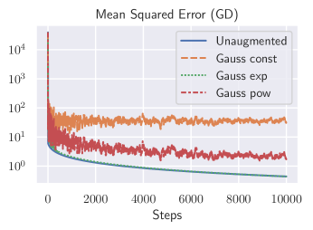
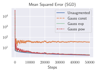
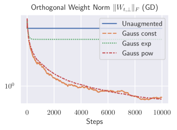
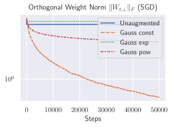
Figure 4.1: MSE and $\|W_{t,\perp}\|_{F}$ for optimization trajectories of GD with additive Gaussian noise augmentation and SGD with additive Gaussian noise augmentation under different augmentation schedules. For both GD and SGD, jointly scheduling learning rate and noise variance to have polynomial decay is necessary for optimization to converge to the minimal norm solution $W_{\min}$. Gauss const, Gauss exp, and Gauss pow have Gaussian noise augmentation with $\sigma_{t}^{2}=2,2e^{-0.02t},2(1+\frac{t}{50})^{-0.33}$, respectively. All other details are given in §4.3.

4.1 Joint schedules for augmented GD with additive noise to converge to $W_{\min}$

We specialize Theorems 3.1 and 3.2 to additive Gaussian noise to show that when the learning rate $\eta_{t}$ and noise strength $\sigma_{t}$ are jointly scheduled to converge to $0$ at appropriate rates, augmented gradient descent can find the minimum norm optimizer $W_{\min}$.

Theorem 4.1.

Consider any joint schedule of the learning rate $\eta_{t}$ and noise variance $\sigma_{t}^{2}$ in which both $\eta_{t}$ and $\sigma_{t}^{2}$ tend to $0$ and $\sigma_{t}$ is non-decreasing. If the joint schedule satisfies

$$\sum_{t=0}^{\infty}\eta_{t}\sigma_{t}^{2}=\infty\qquad\text{and}\qquad\sum_{t=0}^{\infty}\eta_{t}^{2}\sigma_{t}^{2}<\infty,$$ (4.4)

then the weights $W_{t}$ converge in probability to the minimal norm optimum $W_{\text{min}}$ regardless of the initialization. Moreover, the first condition in (4.4) is necessary for $\mathbb{E}[W_{t}]$ to converge to $W_{\min}$.

If we further have $\eta_{t}=\Theta(t^{-x})$ and $\sigma_{t}^{2}=\Theta(t^{-y})$ with $x,y>0$, $x+y<1$, and $2x+y>1$ so that $\eta_{t}$ and $\sigma_{t}^{2}$ satisfy (4.4), then for small $\varepsilon>0$, we have $t^{\min\{y,\frac{1}{2}x\}-\varepsilon}\|W_{t}-W_{\text{min}}\|_{F}\overset{p}{\to}0$.

The conditions of (4.4) require that $\eta_{t}$ and $\sigma_{t}$ be jointly scheduled correctly to ensure convergence to $W_{\min}$ and are akin to the Monro-Robbins conditions (robbins1951stochastic, ) for convergence of stochastic gradient methods. We now give an heuristic explanation for why the first condition from (4.4) is necessary. In this setting, the average trajectory of augmented gradient descent

$$\mathbb{E}[W_{t+1}]=\mathbb{E}[W_{t}]-\eta\nabla_{W}\mathcal{L}_{\sigma_{t}}(W)\big{|}_{W=\mathbb{E}[W_{t}]}$$ (4.5)

is given by gradient descent on the ridge regularized losses $\mathcal{L}_{\sigma_{t}}(W)$. If $\sigma_{t}\equiv\sigma>0$ is constant, then $\mathbb{E}[W_{t}]$ will converge to the unique minimizer $W_{\sigma}^{*}$ of the ridge regularized loss $\mathcal{L}_{\sigma}$. This point $W_{\sigma}^{*}$ has zero orthogonal component, but does not minimize the original loss $\mathcal{L}$.

To instead minimize $\mathcal{L}$, we must choose a schedule satisfying $\sigma_{t}\to 0$. For the expected optimization trajectory to converge to $W_{\min}$ for such a schedule, the matrix $\mathbb{E}[W_{t,\perp}]$ of components of rows of $\mathbb{E}\left[W_{t}\right]$ orthogonal to $V_{\parallel}$ must converge to $0$. The GD steps for this matrix yield

$$\mathbb{E}[W_{t+1,\perp}]=(1-\eta_{t}\sigma_{t}^{2})\mathbb{E}[W_{t,\perp}]=\prod_{s=0}^{t}(1-\eta_{s}\sigma_{s}^{2})\mathbb{E}[W_{0,\perp}].$$ (4.6)

Because $\eta_{t}\sigma_{t}^{2}$ approaches $0$, this implies the necessary condition $\sum_{t=0}^{\infty}\eta_{t}\sigma_{t}^{2}=\infty$ for $\mathbb{E}[W_{t,\perp}]\to 0$.

This argument illustrates a key intuition behind the conditions (4.4). The augmentation strength $\sigma_{t}$ must decay to $0$ to allow convergence to a true minimizer of the training loss, but this convergence must be carefully tuned to allow the implicit regularization of the noising augmentation to kill the orthogonal component of $W_{t}$ in expectation. In a similar manner, the second expression in (4.4) measures the total variance of the gradients and ensures that only a finite amount of noise is injected into the optimization.

Although Theorem 4.1 is stated for additive Gaussian noise, an analogous version holds for arbitrary additive noise with bounded moments. Moreover, optimizing over $x,y$, the fastest rate of convergence guaranteed by Theorem 4.1 is obtained by setting $\eta_{t}=t^{-2/3+\varepsilon},\,\sigma_{t}^{2}=t^{-1/3}$ and results in a $O(t^{-1/3+\varepsilon})$ rate of convergence. It is not evident that this is best possible, however.

4.2 Joint schedules for augmented SGD with additive noise to converge to $W_{\min}$

To conclude our discussion of additive noise augmentations, we present the following result on convergence to $W_{\min}$ in the presence of both Gaussian noise and SGD (where datapoints in each batch are selected with replacement).

Theorem 4.2.

Suppose $\sigma_{t}^{2}\to 0$ is decreasing, $\eta_{t}\to 0$, and we have

$$\sum_{t=0}^{\infty}\eta_{t}\sigma_{t}^{2}=\infty\qquad\text{and}\qquad\sum_{t=0}^{\infty}\eta_{t}^{2}<\infty.$$ (4.7)

Then the trajectory $W_{t}$ of SGD with additive noise converges in probability to $W_{\text{min}}$ for any initialization. If we further have $\eta_{t}=\Theta(t^{-x})$ and $\sigma_{t}^{2}=\Theta(t^{-y})$ with $x>\frac{1}{2}$, $y>0$ and $x+y<1$, then for any $\varepsilon>0$ we have that $t^{\min\{y,\frac{1}{2}x\}-\varepsilon}\|W_{t}-W_{\text{min}}\|_{F}\overset{p}{\to}0$.

Theorem 4.2 is the analog of Theorem 4.1 for mini-batch SGD and provides an example where our framework can handle the composition of two augmentations, namely additive noise and mini-batching. The difference between conditions (4.7) for SGD and (4.4) for GD accounts for the fact that the batch selection changes the scale of the gradient variance at each step. Finally, Theorem 4.2 reveals a qualitative difference between SGD with and without additive noise. If $\eta_{t}$ has power law decay, the convergence of noiseless SGD (Theorem F.1) is exponential in $t$, while Theorem 4.2 gives power law rates.

4.3 Experimental validation

To validate Theorems 4.1 and 4.2, we ran augmented GD and SGD with additive Gaussian noise on $N=100$ simulated datapoints. Inputs were i.i.d. Gaussian vectors in dimension $n=400$, and outputs in dim $p=1$ were generated by a random linear map with i.i.d Gaussian coefficients drawn from $\mathcal{N}(1,1)$. The learning rate followed a fixed polynomially decaying schedule $\eta_{t}=\frac{0.005}{100}\cdot(\text{batch size})\cdot(1+\frac{t}{20})^{-0.66}$, and the batch size used for SGD was $20$. Figure 4.1 shows MSE and $\|W_{t,\perp}\|_{F}$ along a single optimization trajectory with different schedules for the variance $\sigma_{t}^{2}$ used in Gaussian noise augmentation. Complete code to generate this figure is provided in supplement.zip in the supplement. It ran in 30 minutes on a standard laptop CPU.

For both GD and SGD, Figure 4.1 shows that the optimization trajectory reaches $W_{\min}$ only when both learning rate and noise variance decay polynomially to zero. Indeed, Figure 4.1 shows that if $\sigma_{t}^{2}$ is zero (blue) or exponentially decaying (green), then while the MSE tends to zero, the orthogonal component $W_{t,\perp}$ does not tend to zero. Thus these choices of augmentation schedule cause $W_{t}$ to converge to an optimum which does not have minimal norm.

On the other hand, if $\sigma_{t}^{2}$ remains constant (orange), then while $W_{t,\perp}$ tends to zero, the MSE is not minimized. Only by decaying both noise strength and learning rate to $0$ at sufficiently slow polynomial rates (red) prescribed by Theorem 4.1 do we find both MSE and $W_{t,\perp}$ tending to $0$, meaning that augmented (S)GD finds the minimum norm optimum $W_{\min}$ under this choice of parameter scheduling.

5 Special Case: Augmentation with Random Projections

We further illustrate our results by specializing them to a class of augmentations which replace each input $x$ in a batch by its orthogonal projection $\Pi_{t}X$ onto a random subspace. In practice (e.g. when using CutOut (devries2017improved, ) or SpecAugment park2019specaugment ), the subspace is chosen based on a prior about correlations between components of $X$, but we consider the simplified case of a uniformly random subspace of $\mathbb{R}^{n}$ of given dimension.

At each time step $t$ we fix a dimension $k_{t}$ and a fixed $k_{t}$-dimensional subspace $\widetilde{S}_{t}$ of $\mathbb{R}^{n}$. Define the random subspace $S_{t}$ by

$$S_{t}:=Q_{t}(\widetilde{S}_{t})=\{Q_{t}x~{}|~{}x\in\widetilde{S}_{t}\},$$

where $Q_{t}\in O(n)$ is a Haar random orthogonal matrix. Thus, $S_{t}$ is uniformly distributed among all $k_{t}$-dimensional subspaces in $\mathbb{R}^{n}$. At step $t$, we take the augmentation given by

$$X_{t}=\Pi_{t}X\qquad Y_{t}=Y,\qquad\Pi_{t}:=Q_{t}\widetilde{\Pi}_{t}Q_{t}^{\mathsf{T}},$$

where $\widetilde{\Pi}_{t}$ is the orthogonal projection onto $\widetilde{S}_{t}$ and hence $\Pi_{t}$ is the orthogonal projection onto $S_{t}$.

Denoting by $\gamma_{t}=k_{t}/n$ the relative dimension of $S_{t}$, a direct computation (see Lemma E.1) reveals that the proxy loss $\overline{\mathcal{L}}_{t}(W)$ equals $\mathcal{L}(\gamma_{t}W;\mathcal{D})$ plus

$$\frac{1}{N}\frac{\gamma_{t}(1-\gamma_{t})}{n}\|X\|_{F}^{2}\cdot\|W\|_{F}^{2}+\frac{\gamma_{t}(1-\gamma_{t})(1/n-2/n^{2})}{N(1+1/n-2/n^{2})}(\|WX\|_{F}^{2}+\frac{1}{n}\|X\|_{F}^{2}\cdot\|W\|_{F}^{2}).$$ (5.1)

Neglecting terms of order $O(n^{-1})$, this proxy loss applies a Stein-type shrinkage on input data by $\gamma_{t}$ and adds a data-dependent $\ell_{2}$ penalty. For $\gamma_{t}<1$, the minimizer of the proxy loss (5.1) is

$$W_{\gamma_{t}}^{*}=YX^{\mathsf{T}}\Big{(}\frac{\gamma_{t}+1/n-2/n^{2}}{1+1/n-2/n^{2}}XX^{\mathsf{T}}+\frac{1-\gamma_{t}}{1+1/n-2/n^{2}}\frac{\|X\|_{F}^{2}}{n}\operatorname{Id}\Big{)}^{-1}.$$

Again, although $W_{\gamma_{t}}^{*}$ does not minimize the original objective for any $\gamma_{t}<1$, the sequence of these proxy optima converges to the minimal norm optimum in the weak regularization limit. Namely, we have $\lim_{\gamma_{t}\to 1^{-}}W_{\gamma_{t}}^{*}=W_{\min}$. Specializing our general result Theorem 3.1 to this setting, we obtain explicit conditions under which joint schedules of the normalized rank of the projection and the learning rate guarantee convergence to the minimum norm optimizer $W_{\text{min}}$.

Theorem 5.1.

Suppose that $\eta_{t}\to 0,\gamma_{t}\to 1$ with $\gamma_{t}$ non-decreasing and

$$\sum_{t=0}^{\infty}\eta_{t}(1-\gamma_{t})=\infty\,\,\,\text{and}\,\,\,\sum_{t=0}^{\infty}\eta_{t}^{2}(1-\gamma_{t})<\infty.$$ (5.2)

Then, $W_{t}\overset{p}{\to}W_{\text{min}}$. Further, if $\eta_{t}=\Theta(t^{-x})$ and $\gamma_{t}=1-\Theta(t^{-y})$ with $x,y>0$, $x+y<1$, and $2x+y>1$, then for small $\varepsilon>0$, we have that $t^{\min\{y,\frac{1}{2}x\}-\varepsilon}\|W_{t}-W_{\min}\|_{F}\overset{p}{\to}0$.

Comparing the conditions (5.2) of Theorem 5.1 to the conditions (4.4) of Theorem 4.1, we see that $1-\gamma_{t}$ is a measure of the strength of the random projection preconditioning. As in that setting, the fastest rates of convergence guaranteed by Theorem 5.1 are obtained by setting $\eta_{t}=t^{-2/3+\varepsilon}$ and $\gamma_{t}=1-t^{-1/3}$, yielding a $O(t^{-1/3+\varepsilon})$ rate of convergence.

6 Discussion and Limitations

We have presented a theoretical framework to rigorously analyze the effect of data augmentation. As can be seen in our main results, our framework applies to completely general augmentations and relies only on analyzing the first few moments of the augmented dataset. This allows us to handle augmentations as diverse as additive noise and random projections as well as their composition in a uniform manner. We have analyzed some representative examples in detail in this work, but many other commonly used augmentations may be handled similarly: label-preserving transformations (e.g. color jitter, geometric transformations) and Mixup (zhang2017mixup, ), among many others. Another line of investigation left to future work is to compare different methods of combining augmentations such as mixing, alternating, or composing, which often improve performance in the empirical literature (hendrycks2020augmix, ).

Though our results provide a rigorous baseline to compare to more complex settings, the restriction of the present work to linear models is a significant constraint. In future work, we hope to extend our general analysis to models closer to those used in practice. Most importantly, we intend to consider more complex models such as kernels (including the neural tangent kernel) and neural networks by making similar connections to stochastic optimization. In an orthogonal direction, our analysis currently focuses on the mean square loss for regression, and we aim to extend it to other losses such as cross-entropy. Finally, our study has thus far been restricted to the effect of data augmentation on optimization, and it would be of interest to derive consequences for generalization with more complex models. We hope our framework can provide the theoretical underpinnings for a more principled understanding of the effect and practice of data augmentation.

Broader Impact

Our work provides a new theoretical approach to data augmentation for neural networks. By giving a better understanding of how this common practice affects optimization, we hope that it can lead to more robust and interpretable uses of data augmentation in practice. Because our work is theoretical and generic, we do not envision negative impacts aside from those arising from improving learning algorithms in general.

Appendix A Analytic lemmas

In this section, we present several basic lemmas concerning convergence for certain matrix-valued recursions that will be needed to establish our main results. For clarity, we first collect some matrix notations used in this section and throughout the paper.

A.1 Matrix notations

Let $M\in\mathbb{R}^{m\times n}$ be a matrix. We denote its Frobenius norm by $\|M\|_{F}$ and its spectral norm by $\|M\|_{2}$. If $m=n$ so that $M$ is square, we denote by $\operatorname{diag}(M)$ the diagonal matrix with $\operatorname{diag}(M)_{ii}=M_{ii}$. For matrices $A,B,C$ of the appropriate shapes, define

$$A\circ(B\otimes C):=BAC$$ (A.1)

and

$$\text{Var}(A):=\mathbb{E}[A^{\mathsf{T}}\otimes A]-\mathbb{E}[A^{\mathsf{T}}]\otimes\mathbb{E}[A].$$ (A.2)

Notice in particular that

$$\text{tr}[\operatorname{Id}\circ\text{Var}(A)]=\mathbb{E}[\|A-\mathbb{E}[A]\|^{2}_{F}].$$

A.2 One- and two-sided decay

Definition A.1.

Let $A_{t}\in\mathbb{R}^{n\times n}$ be a sequence of independent random non-negative definite matrices with

$$\sup_{t}\left\|A_{t}\right\|\leq 2\quad\text{almost surely},$$

let $B_{t}\in\mathbb{R}^{p\times n}$ be a sequence of arbitrary matrices, and let $C_{t}\in\mathbb{R}^{n\times n}$ be a sequence of non-negative definite matrices. We say that the sequence of matrices $X_{t}\in\mathbb{R}^{p\times n}$ has one-sided decay of type $(\{A_{t}\},\{B_{t}\})$ if it satisfies

$$X_{t+1}=X_{t}(\operatorname{Id}-\mathbb{E}[A_{t}])+B_{t}.$$ (A.3)

We say that a sequence of non-negative definite matrices $Z_{t}\in\mathbb{R}^{n\times n}$ has two-sided decay of type $(\{A_{t}\},\{C_{t}\})$ if it satisfies

$$Z_{t+1}=\mathbb{E}[(\operatorname{Id}-A_{t})Z_{t}(\operatorname{Id}-A_{t})]+C_{t}.$$ (A.4)

Intuitively, if a sequence of matrices $X_{t}$ (resp. $Z_{t}$) satisfies one decay of type $(\{A_{t}\},\{B_{t}\})$ (resp. two-sided decay of type $(\{A_{t}\},\{C_{t}\})$), then in those directions $u\in\mathbb{R}^{n}$ for which $\left\|A_{t}u\right\|$ does not decay too quickly in $t$ we expect that $X_{t}$ (resp. $Z_{t}$) will converge to $0$ provided $B_{t}$ (resp. $C_{t}$) are not too large. More formally, let us define

$$V_{\parallel}:=\bigcap_{t=0}^{\infty}\ker\left[\prod_{s=t}^{\infty}(\operatorname{Id}-\mathbb{E}[A_{s}])\right]=\left\{u\in\mathbb{R}^{n}~{}\bigg{|}~{}\lim_{T\to\infty}\prod_{s=t}^{T}(\operatorname{Id}-\mathbb{E}[A_{s}])u=0,\quad\forall t\geq 1\right\},$$

and let $Q_{\parallel}$ be the orthogonal projection onto $V_{\parallel}$. It is on the space $V_{\parallel}$ that that we expect $X_{t},Z_{t}$ to tend to zero if they satisfy one or two-side decay, and the precise results follows.

A.3 Lemmas on Convergence for Matrices with One and Two-Sided Decay

We state here several results that underpin the proofs of our main results. We begin by giving in Lemmas A.2 and A.3 two slight variations of the same simple argument that matrices with one or two-sided decay converge to zero.

Lemma A.2.

If a sequence $\{X_{t}\}$ has one-sided decay of type $(\{A_{t}\},\{B_{t}\})$ with

$$\sum_{t=0}^{\infty}\|B_{t}\|_{F}<\infty,$$ (A.5)

then $\lim_{t\to\infty}X_{t}Q_{\parallel}=0$.

Proof.

For any $\varepsilon>0$, choose $T_{1}$ so that $\sum_{t=T_{1}}^{\infty}\|B_{t}\|_{F}<\frac{\varepsilon}{2}$ and $T_{2}$ so that for $t>T_{2}$ we have

$$\left\|\Big{(}\prod_{s=T_{1}}^{t}(\operatorname{Id}-\mathbb{E}[A_{s}])\Big{)}Q_{\parallel}\right\|_{2}<\frac{\varepsilon}{2}\frac{1}{\|X_{0}\|_{F}+\sum_{s=0}^{T_{1}-1}\|B_{s}\|_{F}}.$$

By (A.3), we find that

$$X_{t+1}=X_{0}\prod_{s=0}^{t}(\operatorname{Id}-\mathbb{E}[A_{s}])+\sum_{s=0}^{t}B_{s}\prod_{r=s+1}^{t}(\operatorname{Id}-\mathbb{E}[A_{r}]),$$

which implies for $t>T_{2}$ that

$$\|X_{t+1}Q_{\parallel}\|_{F}\leq\|X_{0}\|_{F}\left\|\Big{(}\prod_{s=0}^{t}(\operatorname{Id}-\mathbb{E}[A_{s}])\Big{)}Q_{\parallel}\right\|_{2}+\sum_{s=0}^{t}\|B_{s}\|_{F}\left\|\Big{(}\prod_{r=s+1}^{t}(\operatorname{Id}-\mathbb{E}[A_{r}])\Big{)}Q_{\parallel}\right\|_{2}.$$ (A.6)

Our assumption that $\left\|A_{t}\right\|\leq 2$ almost surely implies that for any $T\leq t$

$$\left\|\Big{(}\prod_{s=0}^{t}(\operatorname{Id}-\mathbb{E}[A_{s}])\Big{)}Q_{\parallel}\right\|_{2}\leq\left\|\Big{(}\prod_{s=0}^{T}(\operatorname{Id}-\mathbb{E}[A_{s}])\Big{)}Q_{\parallel}\right\|_{2}$$

since each term in the product is non-negative-definite. Thus, we find

$$\|X_{t+1}Q_{\parallel}\|_{F}\leq\left[\|X_{0}\|_{F}+\sum_{s=0}^{T_{1}-1}\|B_{s}\|_{F}\right]\left\|\Big{(}\prod_{s=T_{1}}^{t}(\operatorname{Id}-\mathbb{E}[A_{s}])\Big{)}Q_{\parallel}\right\|_{2}+\sum_{s=T_{1}}^{t}\|B_{s}\|_{F}<\varepsilon.$$

Taking $t\to\infty$ and then $\varepsilon\to 0$ implies that $\lim_{t\to\infty}X_{t}Q_{\parallel}=0$, as desired. ∎

Lemma A.3.

If a sequence $\{Z_{t}\}$ has two-sided decay of type $(\{A_{t}\},\{C_{t}\})$ with

$$\lim_{T\to\infty}\mathbb{E}\left[\left\|\Big{(}\prod_{s=t}^{T}(\operatorname{Id}-A_{s})\Big{)}Q_{\parallel}\right\|_{2}^{2}\right]=0\quad\text{ for all $t\geq 0$}$$ (A.7)

and

$$\sum_{t=0}^{\infty}\text{tr}(C_{t})<\infty,$$ (A.8)

then $\lim_{t\to\infty}Q_{\parallel}^{\mathsf{T}}Z_{t}Q_{\parallel}=0$.

Proof.

The proof is essentially identical to that of Lemma A.2. That is, for $\varepsilon>0$, choose $T_{1}$ so that $\sum_{t=T_{1}}^{\infty}\text{tr}(C_{t})<\frac{\varepsilon}{2}$ and choose $T_{2}$ by (A.7) so that for $t>T_{2}$ we have

$$\mathbb{E}\left[\left\|\Big{(}\prod_{s=T_{1}}^{t}(\operatorname{Id}-A_{s})\Big{)}Q_{\parallel}\right\|_{2}^{2}\right]<\frac{\varepsilon}{2}\frac{1}{\text{tr}(Z_{0})+\sum_{s=0}^{T_{1}-1}\text{tr}(C_{s})}.$$

Conjugating (A.4) by $Q_{\parallel}$, we have that

$$Q_{\parallel}^{\mathsf{T}}Z_{t+1}Q_{\parallel}=\mathbb{E}\left[Q_{\parallel}^{\mathsf{T}}\Big{(}\prod_{s=0}^{t}(\operatorname{Id}-A_{s})\Big{)}^{\mathsf{T}}Z_{0}\Big{(}\prod_{s=0}^{t}(\operatorname{Id}-A_{s})\Big{)}Q_{\parallel}\right]\\ +\sum_{s=0}^{t}\mathbb{E}\left[Q_{\parallel}^{\mathsf{T}}\Big{(}\prod_{r=s+1}^{t}(\operatorname{Id}-A_{r})\Big{)}^{\mathsf{T}}C_{s}\Big{(}\prod_{r=s+1}^{t}(\operatorname{Id}-A_{r})\Big{)}Q_{\parallel}\right].$$

Our assumption that $\left\|A_{t}\right\|\leq 2$ almost surely implies that for any $T\leq t$

$$\left\|\Big{(}\prod_{s=0}^{t}(\operatorname{Id}-A_{s})\Big{)}Q\right\|_{2}\leq\left\|\Big{(}\prod_{s=0}^{T}(\operatorname{Id}-A_{s})\Big{)}Q\right\|_{2}.$$

For $t>T_{2}$, this implies by taking trace of both sides that

$$\text{tr}(Q_{\parallel}^{\mathsf{T}}Z_{t+1}Q_{\parallel}) \leq\text{tr}(Z_{0})\mathbb{E}\left[\left\|\Big{(}\prod_{s=0}^{t}(\operatorname{Id}-A_{s})\Big{)}Q_{\parallel}\right\|_{2}^{2}\right]+\sum_{s=0}^{t}\text{tr}(C_{s})\mathbb{E}\left[\left\|\Big{(}\prod_{r=s+1}^{t}(\operatorname{Id}-A_{r})\Big{)}Q_{\parallel}\right\|_{2}^{2}\right]$$ (A.9)

$$\leq\left[\text{tr}(Z_{0})+\sum_{s=0}^{T_{1}-1}\text{tr}(C_{s})\right]\mathbb{E}\left[\left\|\Big{(}\prod_{s=T_{1}}^{t}(\operatorname{Id}-A_{s})\Big{)}Q_{\parallel}\right\|_{2}^{2}\right]+\sum_{s=T_{1}}^{t}\text{tr}(C_{s})$$

$$<\varepsilon,$$

which implies that $\lim_{t\to\infty}Q_{\parallel}^{\mathsf{T}}Z_{t}Q_{\parallel}=0$. ∎

The preceding Lemmas will be used to provide sufficient conditions for augmented gradient descent to converge as in Theorem B.1 below. Since we are also interested in obtaining rates of convergence, we record here two quantitative refinements of the Lemmas above that will be used in the proof of Theorem B.4.

Lemma A.4.

Suppose $\{X_{t}\}$ has one-sided decay of type $(\{A_{t}\},\{B_{t}\})$. Assume also that for some $X\geq 0$ and $C>0$, we have

$$\log\left\|\Big{(}\prod_{r=s}^{t}(\operatorname{Id}-\mathbb{E}[A_{r}])\Big{)}Q_{\parallel}\right\|_{2}<X-C\int_{s}^{t+1}r^{-\alpha}dr$$

and $\|B_{t}\|_{F}=O(t^{-\beta})$ for some $0<\alpha<1<\beta$. Then, $\|X_{t}Q_{\parallel}\|_{F}=O(t^{\alpha-\beta})$.

Proof.

Denote $\gamma_{s,t}:=\int_{s}^{t}r^{-\alpha}dr$. By (A.6), we have for some constants $C_{1},C_{2}>0$ that

$$\|X_{t+1}Q_{\parallel}\|_{F}<C_{1}e^{-C\gamma_{1,t+1}}+C_{2}e^{X}\sum_{s=1}^{t}(1+s)^{-\beta}e^{-C\gamma_{s+1,t+1}}.$$ (A.10)

The first term on the right hand side is exponentially decaying in $t$ since $\gamma_{1,t+1}$ grows polynomially in $t$. To bound the second term, observe that the function

$$f(s):=C\gamma_{s+1,t+1}-\beta\log(s+1)$$

satisfies

$$f^{\prime}(s)\geq 0\quad\Leftrightarrow\quad C(s+1)^{-\alpha}-\frac{\beta}{1+s}\geq 0\quad\Leftrightarrow\quad s\geq\left(\frac{\beta}{C}\right)^{1/(1-\alpha)}=:K.$$

Hence, the summands are monotonically increasing for $s$ greater than a fixed constant $K$ depending only on $\alpha,\beta,C$. Note that

$$\sum_{s=1}^{K}(1+s)^{-\beta}e^{-C\gamma_{s+1,t+1}}\leq Ke^{-C\gamma_{K+1,t+1}}\leq Ke^{-C^{\prime}t^{1-\alpha}}$$

for some $C^{\prime}$ depending only on $\alpha$ and $K$, and hence sum is exponentially decaying in $t$. Further, using an integral comparison, we find

$$\sum_{s=K+1}^{t}(1+s)^{-\beta}e^{-C\gamma_{s+1,t+1}}\leq\int_{K}^{t}(1+s)^{-\beta}e^{-\frac{C}{1-\alpha}\left((t+1)^{1-\alpha}-(s+1)^{1-\alpha}\right)}ds.$$ (A.11)

Changing variables using $u=(1+s)^{1-\alpha}/(1-\alpha)$, the last integral has the form

$$e^{-Cg_{t}}(1-\alpha)^{-\xi}\int_{g_{K}}^{g_{t}}u^{-\xi}e^{Cu}du,\qquad g_{x}:=\frac{(1+x)^{1-\alpha}}{1-\alpha},\,\xi:=\frac{\beta-\alpha}{1-\alpha}.$$ (A.12)

Integrating by parts, we have

$$\int_{g_{K}}^{g_{t}}u^{-\xi}e^{u}du=C^{-1}\xi\int_{g_{K}}^{g_{t}}u^{-\xi-1}e^{Cu}du+(u^{-\xi}e^{Cu})|_{g_{K}}^{g_{t}}$$

Further, since on the range $g_{K}\leq u\leq g_{t}$ the integrand is increasing, we have

$$e^{-Cg_{t}}\xi\int_{g_{K}}^{g_{t}}u^{-\xi-1}e^{Cu}du\leq\xi g_{t}^{-\xi}.$$

Hence, $e^{-Cg_{t}}$ times the integral in (A.12) is bounded above by

$$O(g_{t}^{-\xi})+e^{-Cg_{t}}(u^{-\xi}e^{Cu})|_{g_{K}}^{g_{t}}=O(g_{t}^{-\xi}).$$

Using (A.11) and substituting the previous line into (A.12) yields the estimate

$$\sum_{s=K+1}^{t}(1+s)^{-\beta}e^{-C\gamma_{s+1,t+1}}\leq(1+t)^{-\beta+\alpha},$$

which completes the proof. ∎

Lemma A.5.

Suppose $\{Z_{t}\}$ has two-sided decay of type $(\{A_{t}\},\{C_{t}\})$. Assume also that for some $X\geq 0$ and $C>0$, we have

$$\log\mathbb{E}\left[\left\|\Big{(}\prod_{r=s}^{t}(\operatorname{Id}-A_{r})\Big{)}Q_{\parallel}\right\|_{2}^{2}\right]<X-C\int_{s}^{t+1}r^{-\alpha}dr$$

as well as $\text{tr}(C_{t})=O(t^{-\beta})$ for some $0<\alpha<1<\beta$. Then $\text{tr}(Q_{\parallel}^{T}Z_{t}Q_{\parallel})=O(t^{\alpha-\beta})$.

Proof.

This argument is identical to the proof of Lemma A.4. Indeed, using (A.9) we have that

$$\text{tr}\left(Q_{\parallel}^{T}Z_{t}Q_{\parallel}\right)\leq C_{1}e^{-C\gamma_{1,t+1}}+C_{2}e^{X}\sum_{s=1}^{t}(1+s)^{-\beta}e^{-C\gamma_{s+1,t+1}}.$$

The right hand side of this inequality coincides with the expression on the right hand side of (A.10), which we already bounded by $O(t^{\beta-\alpha})$ in the proof of Lemma A.4. ∎

In what follows, we will use a concentration result for products of matrices from huang2020matrix . Let $Y_{1},\ldots,Y_{n}\in\mathbb{R}^{N\times N}$ be independent random matrices. Suppose that

$$\|\mathbb{E}[Y_{i}]\|_{2}\leq a_{i}\qquad\text{and}\qquad\mathbb{E}\left[\|Y_{i}-\mathbb{E}[Y_{i}]\|_{2}^{2}\right]\leq b_{i}^{2}a_{i}^{2}$$

for some $a_{1},\ldots,a_{n}$ and $b_{1},\ldots,b_{n}$. We will use the following result, which is a specialization of Theorem 5.1 in huang2020matrix for $p=q=2$.

Theorem A.6 (Theorem 5.1 in huang2020matrix ).

For $Z_{0}\in\mathbb{R}^{N\times n}$, the product $Z_{n}=Y_{n}Y_{n-1}\cdots Y_{1}Z_{0}$ satisfies

$$\mathbb{E}\left[\|Z_{n}\|_{2}^{2}\right] \leq e^{\sum_{i=1}^{n}b_{i}^{2}}\prod_{i=1}^{n}a_{i}^{2}\cdot\|Z_{0}\|_{2}^{2}$$

$$\mathbb{E}\left[\|Z_{n}-\mathbb{E}[Z_{n}]\|_{2}^{2}\right] \leq\Big{(}e^{\sum_{i=1}^{n}b_{i}^{2}}-1\Big{)}a_{i}^{2}\cdot\|Z_{0}\|_{2}^{2}.$$

Finally, we collect two simple analytic lemmas for later use.

Lemma A.7.

For any matrix $M\in\mathbb{R}^{m\times n}$, we have that

$$\mathbb{E}[\|M\|_{2}^{2}]\geq\|\mathbb{E}[M]\|_{2}^{2}.$$

Proof.

We find by Cauchy-Schwartz and the convexity of the spectral norm that

$$\mathbb{E}[\|M\|_{2}^{2}]\geq\mathbb{E}[\|M\|_{2}]^{2}\geq\|\mathbb{E}[M]\|_{2}^{2}.\qed$$

Lemma A.8.

For bounded $a_{t}\geq 0$, if we have $\sum_{t=0}^{\infty}a_{t}=\infty$, then for any $C>0$ we have

$$\sum_{t=0}^{\infty}a_{t}e^{-C\sum_{s=0}^{t}a_{s}}<\infty.$$

Proof.

Define $b_{t}:=\sum_{s=0}^{t}a_{s}$ so that

$$S:=\sum_{t=0}^{\infty}a_{t}e^{-C\sum_{s=0}^{t}a_{s}}=\sum_{t=0}^{\infty}(b_{t}-b_{t-1})e^{-Cb_{t}}\leq\int_{0}^{\infty}e^{-Cx}dx<\infty,$$

where we use $\int_{0}^{\infty}e^{-Cx}dx$ to upper bound its right Riemann sum. ∎

Appendix B Analysis of data augmentation as stochastic optimization

In this section, we prove generalizations of our main theoretical results Theorems 3.1 and 3.2 giving Monro-Robbins type conditions for convergence and rates for augmented gradient descent in the linear setting.

B.1 Monro-Robbins type results

To state our general Monro-Robbins type convergence results, let us briefly recall the notation. We consider overparameterized linear regression with loss

$$\mathcal{L}(W;\mathcal{D})=\frac{1}{N}\left\|WX-Y\right\|_{F}^{2},$$

where the dataset $\mathcal{D}$ of size $N$ consists of data matrices $X,Y$ that each have $N$ columns $x_{i}\in\mathbb{R}^{n},y_{i}\in\mathbb{R}^{p}$ with $n>N.$ We optimize $\mathcal{L}(W;\mathcal{D})$ by augmented gradient descent, which means that at each time $t$ we replace $\mathcal{D}=(X,Y)$ by a random dataset $\mathcal{D}_{t}=(X_{t},Y_{t})$. We then take a step

$$W_{t+1}=W_{t}-\eta_{t}\nabla_{W}\mathcal{L}(W_{t};\mathcal{D}_{t})$$

of gradient descent on the resulting randomly augmented loss $\mathcal{L}(W;\mathcal{D}_{t})$ with learning rate $\eta_{t}$. Recall that we set

$$V_{\parallel}:=\text{ column span of $\mathbb{E}[X_{t}X_{t}^{\mathsf{T}}]$}$$

and denoted by $Q_{\parallel}$ the orthogonal projection onto $V_{\parallel}$. As noted in §3, on $V_{\parallel}$ the proxy loss

$$\overline{\mathcal{L}}_{t}=\mathbb{E}\left[\mathcal{L}(W;\mathcal{D}_{t})\right]$$

is strictly convex and has a unique minimum, which is

$$W_{t}^{*}=\mathbb{E}\left[Y_{t}X_{t}^{T}\right](Q_{||}\mathbb{E}\left[X_{t}X_{t}^{\mathsf{T}}\right]Q_{||})^{-1}.$$

The change from one step of augmented GD to the next in these proxy optima is captured by

$$\Xi_{t}^{*}:=W_{t+1}^{*}-W_{t}^{*}.$$

With this notation, we are ready to state Theorems B.1, which gives two different sets of time-varying Monro-Robbins type conditions under which the optimization trajectory $W_{t}$ converges for large $t$. In Theorem B.4, we refine the analysis to additionally give rates of convergence. Note that Theorem B.1 is a generalization of Theorem 3.1 and that Theorem B.4 is a generalization of Theorem 3.2.

Theorem B.1.

Suppose that $V_{\parallel}$ is independent of $t$, that the learning rate satisfies $\eta_{t}\to 0$, that the proxy optima satisfy

$$\sum_{t=0}^{\infty}\|\Xi_{t}^{*}\|_{F}<\infty,$$ (B.1)

ensuring the existence of a limit $W_{\infty}^{*}:=\lim_{t\to\infty}W_{t}^{*}$ and that

$$\sum_{t=0}^{\infty}\eta_{t}\lambda_{\text{min},V_{\parallel}}(\mathbb{E}[X_{t}X_{t}^{\mathsf{T}}])=\infty.$$ (B.2)

Then if either

$$\sum_{t=0}^{\infty}\eta_{t}^{2}\mathbb{E}\left[\|X_{t}X_{t}^{\mathsf{T}}-\mathbb{E}[X_{t}X_{t}^{\mathsf{T}}]\|_{F}^{2}+\|Y_{t}X_{t}^{\mathsf{T}}-\mathbb{E}[Y_{t}X_{t}^{\mathsf{T}}]\|_{F}^{2}\right]<\infty$$ (B.3)

or

$$\sum_{t=0}^{\infty}\eta_{t}^{2}\mathbb{E}\Big{[}\|X_{t}X_{t}^{\mathsf{T}}-\mathbb{E}[X_{t}X_{t}^{\mathsf{T}}]\|_{F}^{2}+\Big{\|}\mathbb{E}[W_{t}](X_{t}X_{t}^{\mathsf{T}}-\mathbb{E}[X_{t}X_{t}^{\mathsf{T}}])-(Y_{t}X_{t}^{\mathsf{T}}-\mathbb{E}[Y_{t}X_{t}^{\mathsf{T}}])\Big{\|}_{F}^{2}\Big{]}<\infty$$ (B.4)

hold, then for any initialization $W_{0}$, we have $W_{t}Q_{\parallel}\overset{p}{\to}W_{\infty}^{*}$.

Remark B.2.

In the general case, the column span $V_{||}$ of $\mathbb{E}[X_{t}X_{t}^{\mathsf{T}}]$ may vary with $t$. This means that some directions in $\mathbb{R}^{n}$ may only have non-zero overlap with $\text{colspan}(\mathbb{E}[X_{t}X_{t}^{\mathsf{T}}])$ for some positive but finite collection of values of $t$. In this case, only finitely many steps of the optimization would move $W_{t}$ in this direction, meaning that we must define a smaller space for convergence. The correct definition of this subspace turns out to be the following

$$V_{\parallel} :=\bigcap_{t=0}^{\infty}\ker\left[\prod_{s=t}^{\infty}\Big{(}\operatorname{Id}-\frac{2\eta_{s}}{N}\mathbb{E}[X_{s}X_{s}^{\mathsf{T}}]\Big{)}\right]$$ (B.5)

$$=\bigcap_{t=0}^{\infty}\left\{u\in\mathbb{R}^{n}~{}\bigg{|}~{}\lim_{T\to\infty}\prod_{s=t}^{T}\Big{(}\operatorname{Id}-\frac{2\eta_{s}}{N}\mathbb{E}[X_{s}X_{s}^{\mathsf{T}}]\Big{)}u=0\right\}.$$

With this re-definition of $V_{||}$ and with $Q_{\parallel}$ still denoting the orthogonal projection to $V_{\parallel}$, Theorem B.1 holds verbatim and with the same proof. Note that if $\eta_{t}\to 0$, $V_{||}=\text{colspan}(\mathbb{E}[X_{t}X_{t}^{\mathsf{T}}])$ is fixed in $t$, and (B.2) holds, this definition of $V_{\parallel}$ reduces to that defined in (3.5).

Remark B.3.

The condition (B.4) can be written in a more conceptual way as

$$\sum_{t=0}^{\infty}\left[\|X_{t}X_{t}^{\mathsf{T}}-\mathbb{E}[X_{t}X_{t}^{\mathsf{T}}]\|_{F}^{2}+\eta_{t}^{2}\text{tr}\left[\operatorname{Id}\circ\text{Var}\Big{(}(\mathbb{E}[W_{t}]X_{t}-Y_{t})X_{t}^{\mathsf{T}}\Big{)}\right]\right]<\infty,$$

where we recognize that $(\mathbb{E}[W_{t}]X_{t}-Y_{t})X_{t}^{\mathsf{T}}$ is precisely the stochastic gradient estimate at time $t$ for the proxy loss $\overline{\mathcal{L}}_{t}$, evaluated at $\mathbb{E}\left[W_{t}\right]$, which is the location at time $t$ for vanilla GD on $\overline{\mathcal{L}}_{t}$ since taking expectations in the GD update equation (3.3) coincides with GD for $\overline{\mathcal{L}}_{t}$. Moreover, condition (B.4) actually implies condition (B.3) (see (B.12) below). The reason we state Theorem B.1 with both conditions, however, is that (B.4) makes explicit reference to the average $\mathbb{E}\left[W_{t}\right]$ of the augmented trajectory. Thus, when applying Theorem B.1 with this weaker condition, one must separately estimate the behavior of this quantity.

Theorem B.1 gave conditions on joint learning rate and data augmentation schedules under which augmented optimization is guaranteed to converge. Our next result proves rates for this convergence.

Theorem B.4.

Suppose that $\eta_{t}\to 0$ and that for some $0<\alpha<1<\beta_{1},\beta_{2}$ and $C_{1},C_{2}>0$, we have

$$\log\mathbb{E}\left[\left\|\Big{(}\prod_{r=s}^{t}\Big{(}\operatorname{Id}-\frac{2\eta_{r}}{N}X_{r}X_{r}^{\mathsf{T}}\Big{)}\Big{)}Q_{\parallel}\right\|_{2}^{2}\right]<C_{1}-C_{2}\int_{s}^{t+1}r^{-\alpha}dr$$ (B.6)

as well as

$$\|\Xi_{t}^{*}\|_{F}=O(t^{-\beta_{1}})$$ (B.7)

and

$$\eta_{t}^{2}\text{tr}\left[\operatorname{Id}\circ\text{Var}(\mathbb{E}[W_{t}]X_{t}X_{t}^{\mathsf{T}}-Y_{t}X_{t}^{\mathsf{T}}\Big{)}\right]=O(t^{-\beta_{2}}).$$ (B.8)

Then, for any initialization $W_{0}$, we have for any $\varepsilon>0$ that

$$t^{\min\{\beta_{1}-1,\frac{\beta_{2}-\alpha}{2}\}-\varepsilon}\|W_{t}Q_{\parallel}-W_{\infty}^{*}\|_{F}\overset{p}{\to}0.$$

Remark B.5.

To reduce Theorem 3.2 to Theorem B.4, we notice that (3.10) and (3.11) mean that Theorem A.6 applies to $Y_{t}=\operatorname{Id}-2\eta_{t}\frac{X_{t}X_{t}^{\mathsf{T}}}{N}$ with $a_{t}=1-\Omega(t^{-\alpha})$ and and $b_{t}^{2}=O(t^{-\gamma})$, thus implying (B.6).

The first step in proving both Theorem B.1 and Theorem B.4 is to obtain recursions for the mean and variance of the difference $W_{t}-W_{t}^{*}$ between the time $t$ proxy optimum and the augmented optimization trajectory at time $t.$ We will then complete the proof of Theorem B.1 in §B.3 and the proof of Theorem B.4 in §B.4.

B.2 Recursion relations for parameter moments

The following proposition shows that difference between the mean augmented dynamics $\mathbb{E}[W_{t}]$ and the time$-t$ optimum $W_{t}^{*}$ satisfies, in the sense of Definition A.1, one-sided decay of type $(\{A_{t}\},\{B_{t}\})$ with

$$A_{t}=\frac{2\eta_{t}}{N}X_{t}X_{t}^{\mathsf{T}},\qquad B_{t}=-\Xi_{t}^{*}.$$

It also shows that the variance of this difference, which is non-negative definite, satisfies two-sided decay of type $(\{A_{t}\},\{C_{t}\})$ with $A_{t}$ as before and

$$C_{t}=\frac{4\eta_{t}^{2}}{N^{2}}\left[\operatorname{Id}\circ\text{Var}\Big{(}\mathbb{E}[W_{t}]X_{t}X_{t}^{\mathsf{T}}-Y_{t}X_{t}^{\mathsf{T}}\Big{)}\right].$$

In terms of the notations of Appendix A.1, we have the following recursions.

Proposition B.6.

The quantity $\mathbb{E}[W_{t}]-W_{t}^{*}$ satisfies

$$\mathbb{E}[W_{t+1}]-W_{t+1}^{*}=(\mathbb{E}[W_{t}]-W_{t}^{*})\Big{(}\operatorname{Id}-\frac{2\eta_{t}}{N}\mathbb{E}[X_{t}X_{t}^{\mathsf{T}}]\Big{)}-\Xi_{t}^{*}$$ (B.9)

and $Z_{t}:=\mathbb{E}[(W_{t}-\mathbb{E}[W_{t}])^{\mathsf{T}}(W_{t}-\mathbb{E}[W_{t}])]$ satisfies

$$Z_{t+1}=\mathbb{E}\left[(\operatorname{Id}-\frac{2\eta_{t}}{N}X_{t}X_{t}^{\mathsf{T}})Z_{t}(\operatorname{Id}-\frac{2\eta_{t}}{N}X_{t}X_{t}^{\mathsf{T}})\right]+\frac{4\eta_{t}^{2}}{N^{2}}\left[\operatorname{Id}\circ\text{Var}\Big{(}\mathbb{E}[W_{t}]X_{t}X_{t}^{\mathsf{T}}-Y_{t}X_{t}^{\mathsf{T}}\Big{)}\right].$$ (B.10)

Proof.

Notice that $\mathbb{E}[X_{t}X_{t}^{\mathsf{T}}]u=0$ if and only if $X_{t}^{\mathsf{T}}u=0$ almost surely, which implies that

$$W_{t}^{*}\mathbb{E}[X_{t}X_{t}^{\mathsf{T}}]=\mathbb{E}[Y_{t}X_{t}^{\mathsf{T}}]\mathbb{E}[X_{t}X_{t}^{\mathsf{T}}]^{+}\mathbb{E}[X_{t}X_{t}^{\mathsf{T}}]=\mathbb{E}[Y_{t}X_{t}^{\mathsf{T}}].$$

Thus, the learning dynamics (3.3) yield

$$\mathbb{E}[W_{t+1}] =\mathbb{E}[W_{t}]-\frac{2\eta_{t}}{N}\Big{(}\mathbb{E}[W_{t}]\mathbb{E}[X_{t}X_{t}^{\mathsf{T}}]-\mathbb{E}[Y_{t}X_{t}^{\mathsf{T}}]\Big{)}$$

$$=\mathbb{E}[W_{t}]-\frac{2\eta_{t}}{N}(\mathbb{E}[W_{t}]-W_{t}^{*})\mathbb{E}[X_{t}X_{t}^{\mathsf{T}}].$$

Subtracting $W_{t+1}^{*}$ from both sides yields (B.9). We now analyze the fluctuations. Writing $\text{Sym}(A):=A+A^{\mathsf{T}}$, we have

$$\mathbb{E}[W_{t+1}]^{\mathsf{T}}\mathbb{E}[W_{t+1}]=\mathbb{E}[W_{t}]^{\mathsf{T}}\mathbb{E}[W_{t}]+\frac{2\eta_{t}}{N}\text{Sym}\Big{(}\mathbb{E}[W_{t}]^{\mathsf{T}}\mathbb{E}[Y_{t}X_{t}^{\mathsf{T}}]-\mathbb{E}[W_{t}]^{\mathsf{T}}\mathbb{E}[W_{t}]\mathbb{E}[X_{t}X_{t}^{\mathsf{T}}]\Big{)}\\ +\frac{4\eta_{t}^{2}}{N^{2}}\Big{(}\mathbb{E}[X_{t}X_{t}^{\mathsf{T}}]\mathbb{E}[W_{t}]^{\mathsf{T}}\mathbb{E}[W_{t}]\mathbb{E}[X_{t}X_{t}^{\mathsf{T}}]+\mathbb{E}[X_{t}Y_{t}^{\mathsf{T}}]\mathbb{E}[Y_{t}X_{t}^{\mathsf{T}}]-\text{Sym}(\mathbb{E}[X_{t}X_{t}^{\mathsf{T}}]\mathbb{E}[W_{t}]^{\mathsf{T}}\mathbb{E}[Y_{t}X_{t}^{\mathsf{T}}])\Big{)}.$$

Similarly, we have that

$$\mathbb{E}[W_{t+1}^{\mathsf{T}}W_{t+1}]=\mathbb{E}[W_{t}^{\mathsf{T}}W_{t}]+\frac{2\eta_{t}}{N}\text{Sym}(\mathbb{E}[W_{t}^{\mathsf{T}}Y_{t}X_{t}^{\mathsf{T}}-W_{t}^{\mathsf{T}}W_{t}X_{t}X_{t}^{\mathsf{T}}])\\ +\frac{4\eta_{t}^{2}}{N^{2}}\mathbb{E}[X_{t}X_{t}^{\mathsf{T}}W_{t}^{\mathsf{T}}W_{t}X_{t}X_{t}^{\mathsf{T}}-\text{Sym}(X_{t}X_{t}^{\mathsf{T}}W_{t}^{\mathsf{T}}Y_{t}X_{t}^{\mathsf{T}})+X_{t}Y_{t}^{\mathsf{T}}Y_{t}X_{t}^{\mathsf{T}}].$$

Noting that $X_{t}$ and $Y_{t}$ are independent of $W_{t}$ and subtracting yields the desired. ∎

B.3 Proof of Theorem B.1

First, by Proposition B.6, we see that $\mathbb{E}[W_{t}]-W_{t}^{*}$ has one-sided decay with

$$A_{t}=2\eta_{t}\frac{X_{t}X_{t}^{\mathsf{T}}}{N}\qquad\text{and}\qquad B_{t}=-\Xi_{t}^{*}.$$

Thus, by Lemma A.2 and (B.1), we find that

$$\lim_{t\to\infty}(\mathbb{E}[W_{t}]Q_{\parallel}-W_{t}^{*})=0,$$ (B.11)

which gives convergence in expectation.

For the second moment, by Proposition B.6, we see that $Z_{t}$ has two-sided decay with

$$A_{t}=2\eta_{t}\frac{X_{t}X_{t}^{\mathsf{T}}}{N}\qquad\text{and}\qquad C_{t}=\frac{4\eta_{t}^{2}}{N^{2}}\left[\operatorname{Id}\circ\text{Var}\Big{(}\mathbb{E}[W_{t}]X_{t}X_{t}^{\mathsf{T}}-Y_{t}X_{t}^{\mathsf{T}}\Big{)}\right].$$

We now verify (A.7) and (A.8) in order to apply Lemma A.3.

For (A.7), for any $\varepsilon>0$, notice that

$$\mathbb{E}[\|A_{s}-\mathbb{E}[A_{s}]\|_{F}^{2}]=\eta_{s}^{2}\mathbb{E}[\|X_{s}X_{s}^{\mathsf{T}}-\mathbb{E}[X_{s}X_{s}^{\mathsf{T}}]\|_{F}^{2}]$$

so by either (B.3) or (B.4) we may choose $T_{1}>t$ so that $\sum_{s=T_{1}}^{\infty}\mathbb{E}[\|A_{s}-\mathbb{E}[A_{s}]\|_{F}^{2}]<\frac{\varepsilon}{2}$. Now choose $T_{2}>T_{1}$ so that for $T>T_{2}$, we have

$$\left\|\Big{(}\prod_{r=T_{1}}^{T}\mathbb{E}[\operatorname{Id}-A_{r}]\Big{)}Q_{\parallel}\right\|_{2}^{2}<\frac{\varepsilon}{2}\frac{1}{\|\prod_{s=t}^{T_{1}-1}\mathbb{E}[\operatorname{Id}-A_{s}]\|_{F}^{2}+\sum_{s=t}^{T_{1}-1}\mathbb{E}[\|A_{s}-\mathbb{E}[A_{s}]\|_{F}^{2}]}.$$

For $T>T_{2}$, we then have

$$\mathbb{E}\left[\left\|\Big{(}\prod_{s=t}^{T}(\operatorname{Id}-A_{s})\Big{)}Q_{\parallel}\right\|_{2}^{2}\right]$$

$$\leq\left\|\Big{(}\prod_{s=t}^{T}\mathbb{E}[\operatorname{Id}-A_{s}]\Big{)}Q_{\parallel}\right\|^{2}+\sum_{s=t}^{T}\mathbb{E}\left[\left\|\prod_{r=t}^{s}(\operatorname{Id}-A_{r})\prod_{r=s+1}^{T}(\operatorname{Id}-\mathbb{E}[A_{r}])Q_{\parallel}\right\|_{F}^{2}-\left\|\prod_{r=t}^{s-1}(\operatorname{Id}-A_{r})\prod_{r=s}^{T}(\operatorname{Id}-\mathbb{E}[A_{r}])Q_{\parallel}\right\|_{F}^{2}\right]$$

$$=\left\|\Big{(}\prod_{s=t}^{T}\mathbb{E}[\operatorname{Id}-A_{s}]\Big{)}Q_{\parallel}\right\|_{F}^{2}+\sum_{s=t}^{T}\mathbb{E}\left[\left\|\prod_{r=t}^{s-1}(\operatorname{Id}-A_{r})(A_{s}-\mathbb{E}[A_{s}])\prod_{r=s+1}^{T}(\operatorname{Id}-\mathbb{E}[A_{r}])Q_{\parallel}\right\|_{F}^{2}\right]$$

$$\leq\left\|\prod_{s=t}^{T_{1}-1}\mathbb{E}[\operatorname{Id}-A_{s}]\right\|^{2}\left\|{}_{F}\Big{(}\prod_{r=T_{1}}^{T}\mathbb{E}[\operatorname{Id}-A_{r}]\Big{)}Q_{\parallel}\right\|_{2}^{2}+\sum_{s=t}^{T}\mathbb{E}[\|A_{s}-\mathbb{E}[A_{s}]\|_{F}^{2}]\left\|\Big{(}\prod_{r=s+1}^{T}\mathbb{E}[\operatorname{Id}-A_{r}]\Big{)}Q_{\parallel}\right\|_{2}^{2}$$

$$\leq\Big{(}\left\|\prod_{s=t}^{T_{1}-1}\mathbb{E}[\operatorname{Id}-A_{s}]\right\|_{F}^{2}+\sum_{s=t}^{T_{1}-1}\mathbb{E}[\|A_{s}-\mathbb{E}[A_{s}]\|_{F}^{2}]\Big{)}\left\|\Big{(}\prod_{r=T_{1}}^{T}\mathbb{E}[\operatorname{Id}-A_{r}]\Big{)}Q_{\parallel}\right\|_{2}^{2}+\sum_{s=T_{1}}^{T}\mathbb{E}[\|A_{s}-\mathbb{E}[A_{s}]\|_{F}^{2}]$$

$$<\varepsilon,$$

which implies (A.7). Condition (A.8) follows from either (B.4) or (B.3) and the bounds

$$\text{tr}(C_{t}) \leq\frac{8\eta_{t}^{2}}{N^{2}}\left(\|\mathbb{E}[W_{t}](X_{t}X_{t}^{\mathsf{T}}-\mathbb{E}[X_{t}X_{t}^{\mathsf{T}}])\|_{F}^{2}+\|Y_{t}X_{t}^{\mathsf{T}}-\mathbb{E}[Y_{t}X_{t}^{\mathsf{T}}]\|_{F}^{2}\right)$$ (B.12)

$$\leq\frac{8\eta_{t}^{2}}{N^{2}}\left(\|\mathbb{E}[W_{t}]\|^{2}\|X_{t}X_{t}^{\mathsf{T}}-\mathbb{E}[X_{t}X_{t}^{\mathsf{T}}]\|_{F}^{2}+\|Y_{t}X_{t}^{\mathsf{T}}-\mathbb{E}[Y_{t}X_{t}^{\mathsf{T}}]\|_{F}^{2}\right),$$

where in the first inequality we use the fact that $\|M_{1}-M_{2}\|_{F}^{2}\leq 2(\|M_{1}\|_{F}^{2}+\|M_{2}\|_{F}^{2})$. Furthermore, iterating (B.9) yields $\|\mathbb{E}[W_{t}]-W_{t}^{*}\|_{F}\leq\|W_{0}-W_{0}^{*}\|_{F}+\sum_{t=0}^{\infty}\|\Xi_{t}^{*}\|_{F}$, which combined with (B.12) and either (B.3) or (B.4) therefore implies (A.8). We conclude by Lemma A.3 that

$$\lim_{t\to\infty}Q_{\parallel}^{\mathsf{T}}Z_{t}Q_{\parallel}=\lim_{t\to\infty}\mathbb{E}[Q_{\parallel}^{\mathsf{T}}(W_{t}-\mathbb{E}[W_{t}])^{\mathsf{T}}(W_{t}-\mathbb{E}[W_{t}])Q_{\parallel}]=0.$$ (B.13)

Together, (B.11) and (B.13) imply that $W_{t}Q_{\parallel}-W_{t}^{*}\overset{p}{\to}0$. The conclusion then follows from the fact that $\lim_{t\to 0}W_{t}^{*}=W_{\infty}^{*}$. This complete the proof of Theorem B.1. $\square$

B.4 Proof of Theorem B.4

By Proposition B.6, $\mathbb{E}[W_{t}]-W_{t}^{*}$ has one-sided decay with

$$A_{t}=\frac{2\eta_{t}}{N}X_{t}X_{t}^{\mathsf{T}},\qquad B_{t}=-\Xi_{t}^{*}.$$

By Lemma A.7 and (B.6), $\mathbb{E}[A_{t}]$ satisfies

$$\log\left\|\prod_{r=s}^{t}\Big{(}\operatorname{Id}-2\eta_{r}\frac{1}{N}\mathbb{E}[X_{r}X_{r}^{\mathsf{T}}]\Big{)}Q_{\parallel}\right\|_{2} \leq\frac{1}{2}\log\mathbb{E}\left[\left\|\Big{(}\prod_{r=s}^{t}\Big{(}\operatorname{Id}-2\eta_{r}\frac{X_{r}X_{r}^{\mathsf{T}}}{N}\Big{)}\Big{)}Q_{\parallel}\right\|_{2}^{2}\right]$$

$$<\frac{C_{1}}{2}-\frac{C_{2}}{2}\int_{s}^{t+1}r^{-\alpha}dr.$$

Applying Lemma A.4 using this bound and (B.7), we find that

$$\|\mathbb{E}[W_{t}]Q_{\parallel}-W_{t}^{*}\|_{F}=O(t^{\alpha-\beta_{1}}).$$

Moreover, because $\|\Xi_{t}^{*}\|_{F}=O(t^{-\beta_{1}})$, we also find that $\|W_{t}^{*}-W_{\infty}^{*}\|_{F}=O(t^{-\beta_{1}+1})$, and hence

$$\|\mathbb{E}[W_{t}]Q_{\parallel}-W_{\infty}^{*}\|_{F}=O(t^{-\beta_{1}+1}).$$

Further, by Proposition B.6, $\mathbb{E}[(W_{t}-\mathbb{E}[W_{t}])^{\mathsf{T}}(W_{t}-\mathbb{E}[W_{t}])]$ has two-sided decay with

$$A_{t}=\frac{2\eta_{t}}{N}X_{t}X_{t}^{\mathsf{T}},\qquad C_{t}=\frac{4\eta_{t}^{2}}{N^{2}}\left[\operatorname{Id}\circ\text{Var}\Big{(}\mathbb{E}[W_{t}]X_{t}X_{t}^{\mathsf{T}}-Y_{t}X_{t}^{\mathsf{T}}\Big{)}\right].$$

Applying Lemma A.5 with (B.6) and (B.8), we find that

$$\mathbb{E}\left[\|(W_{t}-\mathbb{E}[W_{t}])Q_{\parallel}\|_{F}^{2}\right]=O(t^{\alpha-\beta_{2}}).$$

By Chebyshev’s inequality, for any $x>0$ we have

$$\mathbb{P}\Big{(}\|W_{t}Q_{\parallel}-W_{\infty}^{*}\|_{F}\geq O(t^{-\beta_{1}+1})+x\cdot O(t^{\frac{\alpha-\beta_{2}}{2}})\Big{)}\leq x^{-2}.$$

For any $\varepsilon>0$, choosing $x=t^{\delta}$ for small $0<\delta<\varepsilon$ we find as desired that

$$t^{\min\{\beta_{1}-1,\frac{\beta_{2}-\alpha}{2}\}-\varepsilon}\|W_{t}Q_{\parallel}-W_{\infty}^{*}\|_{F}\overset{p}{\to}0,$$

thus completing the proof of Theorem B.4. $\square$

Appendix C Intrinsic time

Theorem 3.2 measures rates in terms of optimization steps $t$, but a different measurement of time called the intrinsic time of the optimization will be more suitable for measuring the behavior of optimization quantities. This was introduced for SGD in smith2018bayesian ; smith2018don , and we now generalize it to our broader setting. For gradient descent on a loss $\mathcal{L}$, the intrinsic time is a quantity which increments by $\eta\lambda_{\text{min}}(H)$ for a optimization step with learning rate $\eta$ at a point where $\mathcal{L}$ has Hessian $H$. When specialized to our setting, it is given by

$$\tau(t):=\sum_{s=0}^{t-1}\frac{2\eta_{s}}{N}\lambda_{\text{min},V_{\parallel}}(\mathbb{E}[X_{s}X_{s}^{\mathsf{T}}]).$$ (C.1)

Notice that intrinsic time of augmented optimization for the sequence of proxy losses $\overline{\mathcal{L}}_{s}$ appears in Theorems 3.1 and 3.2, which require via conditions (3.8) and (3.11) that the intrinsic time tends to infinity as the number of optimization steps grows.

Intrinsic time will be a sensible variable in which to measure the behavior of quantities such as the fluctuations of the optimization path $f(t):=\mathbb{E}[\|(W_{t}-\mathbb{E}[W_{t}])Q_{\parallel}\|_{F}^{2}]$. In the proofs of Theorems 3.1 and 3.2, we show that the fluctuations satisfy an inequality of the form

$$f(t+1)\leq f(t)(1-a(t))^{2}+b(t)$$ (C.2)

for $a(t):=2\eta_{t}\frac{1}{N}\lambda_{\text{min},V_{\parallel}}(\mathbb{E}[X_{t}X_{t}^{\mathsf{T}}])$ and $b(t):=\text{Var}[\left\|\eta_{t}\nabla_{W}\mathcal{L}(W_{t})\right\|_{F}]$ so that $\tau(t)=\sum_{s=0}^{t-1}a(s)$. Iterating the recursion (C.2) shows that

$$f(t) \leq f(0)\prod_{s=0}^{t-1}(1-a(s))^{2}+\sum_{s=0}^{t-1}b(s)\prod_{r=s+1}^{t-1}(1-a(r))^{2}$$

$$\leq e^{-2\tau(t)}f(0)+\sum_{s=0}^{t-1}\frac{b(s)}{a(s)}e^{2\tau(s+1)-2\tau(t)}(\tau(s+1)-\tau(s)).$$

Changing variables to $\tau:=\tau(t)$ and defining $A(\tau)$, $B(\tau)$, and $F(\tau)$ by $A(\tau(t))=a(t)$, $B(\tau(t))=b(t)$, and $F(\tau(t))=f(t)$, we find by replacing a right Riemann sum by an integral that

$$F(\tau)\precsim e^{-2\tau}\left[F(0)+\int_{0}^{\tau}\frac{B(\sigma)}{A(\sigma)}e^{2\sigma}d\sigma\right].$$ (C.3)

In order for the result of optimization to be independent of the starting point, by (C.3) we must have $\tau\to\infty$ to remove the dependence on $F(0)$; this provides one explanation for the appearance of $\tau$ in condition (3.8). Further, (C.3) implies that the fluctuations at an intrinsic time are bounded by an integral against the function $\frac{B(\sigma)}{A(\sigma)}$ which depends only on the ratio of $A(\sigma)$ and $B(\sigma)$.

In the case of minibatch SGD, our proof of Theorem F.1 shows the intrinsic time is $\tau(t)=\sum_{s=0}^{t-1}2\eta_{s}\frac{1}{N}\lambda_{\text{min},V_{\parallel}}(XX^{\mathsf{T}})$ and the ratio $\frac{b(t)}{a(t)}$ in (C.3) is by (F.5) bounded uniformly by $\frac{b(t)}{a(t)}\leq C\cdot\frac{\eta_{t}}{B_{t}}$ for a constant $C>0$. Thus, keeping $\frac{b(t)}{a(t)}$ fixed as a function of $\tau$ suggests the “linear scaling” $\eta_{t}\propto B_{t}$ used empirically in goyal2017accurate and proposed via an heuristic SDE limit in smith2018don .

Appendix D Analysis of Noising Augmentations

In this section, we give a full analysis of the noising augmentations presented in Section 4. Let us briefly recall the notation. As before, we consider overparameterized linear regression with loss

$$\mathcal{L}(W;\mathcal{D})=\frac{1}{N}\left\|WX-Y\right\|_{F}^{2},$$

where the dataset $\mathcal{D}$ of size $N$ consists of data matrices $X,Y$ that each have $N$ columns $x_{i}\in\mathbb{R}^{n},y_{i}\in\mathbb{R}^{p}$ with $n>N.$ We optimize $\mathcal{L}(W;\mathcal{D})$ by augmented gradient descent or augmented stochastic gradient descent with additive Gaussian noise. This means that at each time $t$ we replace $\mathcal{D}=(X,Y)$ by a random batch $\mathcal{D}_{t}=(X_{t},Y)$ of size $B_{t}$, where the columns $x_{i,t}$ of $X_{t}$ are

$$x_{i,t}=x_{i}+\sigma_{t}G_{i,t},\qquad G_{i,t}\sim\mathcal{N}(0,1)\text{ i.i.d.}$$

In the case of gradient descent, the batch consists of the entire dataset, and the resulting data matrices are

$$X_{t}=X+\sigma_{t}G_{t}\qquad\text{and}\qquad Y_{t}=Y.$$

In the case of stochastic gradient descent, the batch consists of $B_{t}$ datapoints chosen uniformly at random with replacement, and the resulting data matrices are

$$X_{t}=c_{t}(XA_{t}+\sigma_{t}G_{t})\qquad\text{and}\qquad Y_{t}=c_{t}YA_{t},$$

where $c_{t}=\sqrt{N/B_{t}}$, $A_{t}\in\mathbb{R}^{N\times B_{t}}$ has i.i.d. columns with a single non-zero entry equal to $1$, and $G_{t}\in\mathbb{R}^{n\times B_{t}}$ has i.i.d. Gaussian entries. In both cases, the proxy loss is

$$\overline{\mathcal{L}}_{t}(W):=\frac{1}{N}\|Y-WX\|_{F}^{2}+\sigma_{t}^{2}\|W\|_{F}^{2},$$

which has ridge minimizer

$$W_{t}^{*}=YX^{\mathsf{T}}(XX^{\mathsf{T}}+\sigma_{t}^{2}N\cdot\operatorname{Id}_{n\times n})^{-1},$$

and the space $V_{\parallel}:=\text{ column span of $\mathbb{E}[X_{t}X_{t}^{\mathsf{T}}]$}$ is all of $\mathbb{R}^{n}$. We now separately analyze the cases of GD and SGD in Theorems 4.1 and Theorem 4.2, respectively.

D.1 Proof of Theorem 4.1 for GD

We begin by proving convergence without rates. For this, we seek to show that if $\sigma_{t}^{2},\eta_{t}\to 0$ with $\sigma_{t}^{2}$ non-increasing and

$$\sum_{t=0}^{\infty}\eta_{t}\sigma_{t}^{2}=\infty\qquad\text{and}\qquad\sum_{t=0}^{\infty}\eta_{t}^{2}\sigma_{t}^{2}<\infty,$$ (D.1)

then, $W_{t}\overset{p}{\to}W_{\text{min}}$. We will do this by applying Theorem 3.1, so we check that our assumptions imply the hypotheses of these theorems. For Theorem 3.1, we directly compute

$$\mathbb{E}[Y_{t}X_{t}^{\mathsf{T}}]=YX^{\mathsf{T}}\qquad\text{and}\qquad\mathbb{E}[X_{t}X_{t}^{\mathsf{T}}]=XX^{\mathsf{T}}+\sigma_{t}^{2}N\cdot\operatorname{Id}_{n\times n}$$

and

$$\mathbb{E}[X_{t}X_{t}^{\mathsf{T}}X_{t}] =XX^{\mathsf{T}}X+\sigma_{t}^{2}(N+n+1)X$$

$$\mathbb{E}[X_{t}X_{t}^{\mathsf{T}}X_{t}X_{t}^{\mathsf{T}}] =XX^{\mathsf{T}}XX^{\mathsf{T}}+\sigma_{t}^{2}\Big{(}(2N+n+2)XX^{\mathsf{T}}+\text{tr}(XX^{\mathsf{T}})\operatorname{Id}_{n\times n}\Big{)}+\sigma_{t}^{4}N(N+n+1)\operatorname{Id}_{n\times n}.$$

We also find that

$$\|\Xi_{t}^{*}\|_{F} =|\sigma_{t}^{2}-\sigma_{t+1}^{2}|N\left\|YX^{\mathsf{T}}\Big{(}XX^{\mathsf{T}}+\sigma_{t}^{2}N\cdot\operatorname{Id}_{n\times n}\Big{)}^{-1}\Big{(}XX^{\mathsf{T}}+\sigma_{t+1}^{2}N\cdot\operatorname{Id}_{n\times n}\Big{)}^{-1}\right\|_{F}$$

$$\leq|\sigma_{t}^{2}-\sigma_{t+1}^{2}|N\|YX^{\mathsf{T}}[(XX^{\mathsf{T}})^{+}]^{2}\|_{F}.$$

Thus, because $\sigma_{t}^{2}$ is decreasing, we see that the hypothesis (3.7) of Theorem 3.1 indeed holds. Further, we note that

$$\sum_{t=0}^{\infty}\eta_{t}^{2}\mathbb{E}\left[\|X_{t}X_{t}^{\mathsf{T}}-\mathbb{E}[X_{t}X_{t}^{\mathsf{T}}]\|_{F}^{2}+\|Y_{t}X_{t}^{\mathsf{T}}-\mathbb{E}[Y_{t}X_{t}^{\mathsf{T}}]\|_{F}^{2}\right]\\ =\sum_{t=0}^{\infty}\eta_{t}^{2}\sigma_{t}^{2}\Big{(}2(n+1)\|X\|_{F}^{2}+N\|Y\|_{F}^{2}+\sigma_{t}^{2}Nn(n+1)\Big{)}=O\left(\sum_{t=0}^{\infty}\eta_{t}^{2}\sigma_{t}^{2}\right),$$

which by (D.1) implies (B.3). Theorem 3.1 and the fact that $\lim_{t\to\infty}W_{t}^{*}=W_{\text{min}}$ therefore yield that $W_{t}\overset{p}{\to}W_{\text{min}}$.

We now prove convergence with rates, we aim to show that if $\eta_{t}=\Theta(t^{-x})$ and $\sigma_{t}^{2}=\Theta(t^{-y})$ with $x,y>0$, $x+y<1$, and $2x+y>1$, then for any $\varepsilon>0$, we have that

$$t^{\min\{y,\frac{1}{2}x\}-\varepsilon}\|W_{t}-W_{\text{min}}\|_{F}\overset{p}{\to}0.$$

We now check the hypotheses for and apply Theorem B.4. For (B.6), notice that $Y_{r}=\operatorname{Id}-2\eta_{r}\frac{X_{r}X_{r}^{\mathsf{T}}}{N}$ satisfies the hypotheses of Theorem A.6 with $a_{r}=1-2\eta_{r}\sigma_{r}^{2}$ and $b_{r}^{2}=\frac{\eta_{r}^{2}\sigma_{r}^{2}}{a_{r}^{2}}\Big{(}2(n+1)\|X\|_{F}^{2}+\sigma_{r}^{2}Nn(n+1)\Big{)}$. Thus, by Theorem A.6 and the fact that $\eta_{t}=\Theta(t^{-x})$ and $\sigma_{t}^{2}=\Theta(t^{-y})$, we find for some $C_{1},C_{2}>0$ that

$$\log\mathbb{E}\left[\left\|\prod_{r=s}^{t}(\operatorname{Id}-2\eta_{r}\frac{X_{r}X_{r}^{\mathsf{T}}}{N})\right\|^{2}_{2}\right]\leq\sum_{r=s}^{t}b_{r}^{2}+2\sum_{r=s}^{t}\log(1-2\eta_{r}\sigma_{r}^{2})\leq C_{1}-C_{2}\int_{s}^{t+1}r^{-x-y}dr.$$

For (B.7), we find that

$$\|\Xi_{t}^{*}\|_{F}\leq|\sigma_{t}^{2}-\sigma_{t+1}^{2}|N\|YX^{\mathsf{T}}[(XX^{\mathsf{T}})^{+}]^{2}\|_{F}=O(t^{-y-1}).$$

Finally, for (B.8), we find that

$$\eta_{t}^{2} \text{tr}\left[\operatorname{Id}\circ\text{Var}\Big{(}\mathbb{E}[W_{t}]X_{t}X_{t}^{\mathsf{T}}-Y_{t}X_{t}^{\mathsf{T}}\Big{)}\right]=\eta_{t}^{2}\mathbb{E}\Big{[}\|\mathbb{E}[W_{t}](X_{t}X_{t}^{\mathsf{T}}-\mathbb{E}[X_{t}X_{t}^{\mathsf{T}}])-(Y_{t}X_{t}^{\mathsf{T}}-\mathbb{E}[Y_{t}X_{t}^{\mathsf{T}}])\|_{F}^{2}\Big{]}$$

$$\leq 2\eta_{t}^{2}\mathbb{E}\Big{[}\|\mathbb{E}[W_{t}](X_{t}X_{t}^{\mathsf{T}}-\mathbb{E}[X_{t}X_{t}^{\mathsf{T}}])\|_{F}^{2}+\|Y_{t}X_{t}^{\mathsf{T}}-\mathbb{E}[Y_{t}X_{t}^{\mathsf{T}}]\|_{F}^{2}\Big{]}$$

$$\leq 2\eta_{t}^{2}\Big{(}\|\mathbb{E}[W_{t}]\|_{F}^{2}\mathbb{E}[\|X_{t}X_{t}^{\mathsf{T}}-\mathbb{E}[X_{t}X_{t}^{\mathsf{T}}]\|_{F}^{2}]+\|Y_{t}X_{t}^{\mathsf{T}}-\mathbb{E}[Y_{t}X_{t}^{\mathsf{T}}]\|_{F}^{2}\Big{)}$$

$$=O(t^{-2x-y}).$$

Noting finally that $\|W_{t}^{*}-W_{\text{min}}\|_{F}=O(\sigma_{t}^{2})=O(t^{-y})$, we apply Theorem B.4 with $\alpha=x+y$, $\beta_{1}=y+1$, and $\beta_{2}=2x+y$ to obtain the desired estimates. This concludes the proof of Theorem 4.1. $\square$

D.2 Proof of Theorem 4.2 for SGD

We now prove Theorem 4.2 for SGD. As before, we will apply Theorems 3.1 and B.4. To check the hypotheses of these theorems, we will use the following expressions for moments of the augmented data matrices.

Lemma D.1.

We have

$$\mathbb{E}[Y_{t}X_{t}^{\mathsf{T}}]=YX^{\mathsf{T}}\qquad\text{and}\qquad\mathbb{E}[X_{t}X_{t}^{\mathsf{T}}]=XX^{\mathsf{T}}+\sigma_{t}^{2}N\operatorname{Id}_{n\times n}.$$ (D.2)

Moreover,

$$\mathbb{E}[Y_{t}X_{t}^{\mathsf{T}}X_{t}Y_{t}^{\mathsf{T}}] =c_{t}^{4}\mathbb{E}[YA_{t}A_{t}^{\mathsf{T}}X^{\mathsf{T}}XA_{t}A_{t}^{\mathsf{T}}Y^{\mathsf{T}}+\sigma_{t}^{2}YA_{t}G_{t}^{\mathsf{T}}G_{t}A_{t}^{\mathsf{T}}Y^{\mathsf{T}}]$$

$$=\frac{N}{B_{t}}Y\operatorname{diag}(X^{\mathsf{T}}X)Y^{\mathsf{T}}+\frac{B_{t}-1}{B_{t}}YX^{\mathsf{T}}XY^{\mathsf{T}}+\sigma_{t}^{2}NYY^{\mathsf{T}}$$

$$\mathbb{E}[Y_{t}X_{t}^{\mathsf{T}}X_{t}X_{t}^{\mathsf{T}}] =c_{t}^{4}\mathbb{E}[YA_{t}A_{t}^{\mathsf{T}}X^{\mathsf{T}}XA_{t}A_{t}^{\mathsf{T}}X^{\mathsf{T}}+\sigma_{t}^{2}YA_{t}G_{t}^{\mathsf{T}}G_{t}A_{t}^{\mathsf{T}}X^{\mathsf{T}}$$

$$\phantom{==}+\sigma_{t}^{2}YA_{t}G_{t}^{\mathsf{T}}XA_{t}G_{t}^{\mathsf{T}}+\sigma_{t}^{2}YA_{t}A_{t}^{\mathsf{T}}X^{\mathsf{T}}G_{t}G_{t}^{\mathsf{T}}]$$

$$=\frac{N}{B_{t}}Y\operatorname{diag}(X^{\mathsf{T}}X)X^{\mathsf{T}}+\frac{B_{t}-1}{B_{t}}YX^{\mathsf{T}}XX^{\mathsf{T}}+\sigma_{t}^{2}(N+\frac{n+1}{B_{t}/N})YX^{\mathsf{T}}$$

$$\mathbb{E}[X_{t}X_{t}^{\mathsf{T}}X_{t}X_{t}^{\mathsf{T}}] =c_{t}^{4}\mathbb{E}[XA_{t}A_{t}^{\mathsf{T}}X^{\mathsf{T}}XA_{t}A_{t}^{\mathsf{T}}X^{\mathsf{T}}+\sigma_{t}^{2}G_{t}G_{t}^{\mathsf{T}}XA_{t}A_{t}^{\mathsf{T}}X^{\mathsf{T}}+\sigma_{t}^{2}XA_{t}G_{t}^{\mathsf{T}}G_{t}A_{t}^{\mathsf{T}}X^{\mathsf{T}}$$

$$\phantom{==}+\sigma_{t}^{2}XA_{t}A_{t}^{\mathsf{T}}X^{\mathsf{T}}G_{t}G_{t}^{\mathsf{T}}+\sigma_{t}^{2}G_{t}A_{t}^{\mathsf{T}}X^{\mathsf{T}}G_{t}A_{t}^{\mathsf{T}}X^{\mathsf{T}}+\sigma_{t}^{2}XA_{t}G_{t}^{\mathsf{T}}XA_{t}G_{t}^{\mathsf{T}}$$

$$\phantom{==}+\sigma_{t}^{2}G_{t}A_{t}^{\mathsf{T}}X^{\mathsf{T}}XA_{t}G_{t}^{\mathsf{T}}+\sigma_{t}^{4}G_{t}G_{t}^{\mathsf{T}}G_{t}G_{t}^{\mathsf{T}}]$$

$$=\frac{N}{B_{t}}X\operatorname{diag}(X^{\mathsf{T}}X)X^{\mathsf{T}}+\frac{B_{t}-1}{B_{t}}XX^{\mathsf{T}}XX^{\mathsf{T}}+\sigma_{t}^{2}(2N+\frac{n+2}{B_{t}/N})XX^{\mathsf{T}}$$

$$\phantom{==}+\sigma_{t}^{2}\frac{N}{B_{t}}\text{tr}(XX^{\mathsf{T}})\operatorname{Id}_{n\times n}+\sigma_{t}^{4}N(N+\frac{n+1}{B_{t}/N})\operatorname{Id}_{n\times n}.$$

Proof.

All these formulas are obtained by direct, if slightly tedious, computation. ∎

With these expressions in hand, we now check the conditions of Theorem 3.1. First, by the Sherman-Morrison-Woodbury matrix inversion formula, we have

$$\|\Xi_{t}^{*}\|_{F} =|\sigma_{t}^{2}N-\sigma_{t+1}^{2}N|\left\|YX^{\mathsf{T}}(XX^{\mathsf{T}}+\sigma_{t}^{2}N\cdot\operatorname{Id}_{n\times n})^{-1}(XX^{\mathsf{T}}+\sigma_{t+1}^{2}N\cdot\operatorname{Id}_{n\times n})^{-1}\right\|_{F}$$ (D.3)

$$\leq N|\sigma_{t}^{2}-\sigma_{t+1}^{2}|\left\|YX^{\mathsf{T}}[(XX^{\mathsf{T}})^{+}]^{2}\right\|_{F}.$$

Because $\sigma_{t}^{2}$ is non-increasing, this implies (3.7). Next, by Lemma D.1 we have that

$$\sum_{t=0}^{\infty}\eta_{t}\lambda_{\text{min},V_{\parallel}}(\mathbb{E}[X_{t}X_{t}^{\mathsf{T}}])\geq\sum_{t=0}^{\infty}\eta_{t}\sigma_{t}^{2}=\infty$$

by the first given condition in (4.7), which verifies (3.8). Finally, by Lemma D.1, we may compute

$$\mathbb{E}\left[\left\|X_{t}X_{t}^{\mathsf{T}}-\mathbb{E}\left[X_{t}X_{t}^{\mathsf{T}}\right]\right\|_{F}^{2}\right]\\ =\frac{1}{B_{t}}\text{tr}\Big{(}X(N\operatorname{diag}(X^{\mathsf{T}}X)-X^{\mathsf{T}}X)X^{\mathsf{T}}\Big{)}+2\sigma_{t}^{2}\frac{n+1}{B_{t}/N}\text{tr}(XX^{\mathsf{T}})+\sigma_{t}^{4}\frac{Nn(n+1)}{B_{t}/N}$$

and

$$\mathbb{E}\left[\|Y_{t}X_{t}^{\mathsf{T}}-\mathbb{E}[Y_{t}X_{t}^{\mathsf{T}}]\|_{F}^{2}\right]=\frac{1}{B_{t}}\text{tr}\Big{(}Y(N\operatorname{diag}(X^{\mathsf{T}}X)-X^{\mathsf{T}}X)Y^{\mathsf{T}}\Big{)}+\sigma_{t}^{2}N\text{tr}(YY^{\mathsf{T}}).$$

Together, these imply that for some constant $C>0$, we have that

$$\sum_{t=0}^{\infty}\eta_{t}^{2}\left[\mathbb{E}\left[\left\|X_{t}X_{t}^{\mathsf{T}}-\mathbb{E}\left[X_{t}X_{t}^{\mathsf{T}}\right]\right\|_{F}^{2}\right]+\mathbb{E}\left[\left\|Y_{t}X_{t}^{\mathsf{T}}-\mathbb{E}[Y_{t}X_{t}^{\mathsf{T}}]\right\|_{F}^{2}\right]\right]\leq\sum_{t=0}^{\infty}C\eta_{t}^{2}<\infty$$

by the second given condition in (4.7), which verifies (3.9). Thus the conditions of Theorem 3.1 apply, which shows that $W_{t}\overset{p}{\to}W_{\text{min}}$, as desired.

For rates of convergence, we check the conditions of Theorem B.4. For (B.6), we will apply Theorem A.6 to bound $\log\mathbb{E}\left\|\prod_{r=s}^{t}\left(\operatorname{Id}-\frac{2\eta_{r}}{N}X_{r}X_{r}^{\mathsf{T}}\right)\right\|_{2}^{2}$. By the second moment expression $\mathbb{E}[X_{r}X_{r}^{\mathsf{T}}]=XX^{\mathsf{T}}+\sigma_{r}^{2}N\operatorname{Id}_{n\times n}$, we find that

$$\left\|\mathbb{E}\left[\operatorname{Id}-\frac{2\eta_{r}}{N}X_{r}X_{r}^{\mathsf{T}}\right]\right\|_{2}=1-2\eta_{r}\sigma_{r}^{2}.$$

Moreover, by Lemma D.1, for some constant $C>0$ we have

$$\mathbb{E}\left[\left\|\operatorname{Id}-\frac{2\eta_{r}}{N}X_{r}X_{r}^{\mathsf{T}}-\mathbb{E}\left[\operatorname{Id}-\frac{2\eta_{r}}{N}X_{r}X_{r}^{\mathsf{T}}\right]\right\|_{2}^{2}\right]$$

$$=\frac{4\eta_{r}^{2}}{N^{2}}\mathbb{E}\left[\left\|X_{r}X_{r}^{\mathsf{T}}-\mathbb{E}\left[X_{r}X_{r}^{\mathsf{T}}\right]\right\|_{2}^{2}\right]$$

$$\leq\frac{4\eta_{r}^{2}}{N^{2}}\left[\frac{1}{B_{t}}\text{tr}\Big{(}X(N\operatorname{diag}(X^{\mathsf{T}}X)-X^{\mathsf{T}}X)X^{\mathsf{T}}\Big{)}+2\sigma_{t}^{2}\frac{n+1}{B_{t}/N}\text{tr}(XX^{\mathsf{T}})+\sigma_{t}^{4}\frac{Nn(n+1)}{B_{t}/N}\right]$$

$$\leq C\eta_{r}^{2}.$$

Applying Theorem A.6 with $a_{r}=1-2\eta_{r}\sigma_{r}^{2}$ and $b_{r}^{2}=\frac{C\eta_{r}^{2}}{a_{r}^{2}}$, we find that

$$\log\mathbb{E}\left\|\prod_{r=s}^{t}\left(\operatorname{Id}-\frac{2\eta_{r}}{N}X_{r}X_{r}^{\mathsf{T}}\right)\right\|_{2}^{2} \leq\sum_{r=s}^{t}\frac{C\eta_{r}^{2}}{a_{r}^{2}}+2\log\left(\prod_{r=s}^{t}\left(1-2\eta_{r}\sigma_{r}^{2}\right)\right)$$

$$\leq\sum_{r=s}^{t}\frac{C\eta_{r}^{2}}{a_{r}^{2}}-4\sum_{r=s}^{t}\eta_{r}\sigma_{r}^{2}.$$

Because $\eta_{r}=\Theta(r^{-x})$ and $\sigma_{r}^{2}=\Theta(r^{-y})$, we obtain (B.6) with $\alpha=x+y$, $C_{1}=\sum_{r=0}^{\infty}\frac{C\eta_{r}^{2}}{a_{r}^{2}}$, and some $C_{2}>0$, where $C_{1}$ is finite because $x>\frac{1}{2}$. Next, (B.7) holds for $\beta_{1}=-y-1$ by (D.3). Finally, it remains to bound

$$\eta_{t}^{2}\text{tr}\left[\operatorname{Id}\circ\text{Var}(\mathbb{E}[W_{t}]X_{t}X_{t}^{\mathsf{T}}-Y_{t}X_{t}^{\mathsf{T}}\Big{)}\right]$$

to verify (B.8). Again using D.1 and noting that $W_{\text{min}}X=Y$, we find

$$\eta_{t}^{2} \text{tr}\left[\operatorname{Id}\circ\text{Var}(\mathbb{E}[W_{t}]X_{t}X_{t}^{\mathsf{T}}-Y_{t}X_{t}^{\mathsf{T}})\right]$$

$$=\eta_{t}^{2}\text{tr}\Big{(}\frac{1}{B_{t}}\mathbb{E}[W_{t}]X(N\operatorname{diag}(X^{\mathsf{T}}X)-X^{\mathsf{T}}X)X^{\mathsf{T}}\mathbb{E}[W_{t}]^{\mathsf{T}}$$

$$\phantom{==}+2\sigma_{t}^{2}\frac{n+1}{B_{t}/N}\mathbb{E}[W_{t}]XX^{\mathsf{T}}\mathbb{E}[W_{t}]^{\mathsf{T}}+(\sigma_{t}^{2}\frac{N}{B_{t}}\text{tr}(XX^{\mathsf{T}})+\sigma_{t}^{4}N\frac{n+1}{B_{t}/N})\mathbb{E}[W_{t}]\mathbb{E}[W_{t}]^{\mathsf{T}}\Big{)}$$

$$\phantom{==}-2\eta_{t}^{2}\text{tr}\Big{(}\frac{1}{B_{t}}Y(N\operatorname{diag}(X^{\mathsf{T}}X)-X^{\mathsf{T}}X)X^{\mathsf{T}}\mathbb{E}[W_{t}]^{\mathsf{T}}+\sigma_{t}^{2}\frac{n+1}{B_{t}/N}YX^{\mathsf{T}}\mathbb{E}[W_{t}]^{\mathsf{T}}\Big{)}$$

$$\phantom{==}+\eta_{t}^{2}\text{tr}\Big{(}\frac{1}{B_{t}}Y(N\operatorname{diag}(X^{\mathsf{T}}X)-X^{\mathsf{T}}X)Y^{\mathsf{T}}+\sigma_{t}^{2}NYY^{\mathsf{T}}\Big{)}$$

$$\leq C\eta_{t}^{2}(\sigma_{t}^{2}+\left\|\Delta_{t}\right\|_{F}^{2})$$

for some $C>0$ and $\Delta_{t}:=\mathbb{E}[W_{t}]-W_{\text{min}}$. Define also $\Delta_{t}^{\prime}:=\mathbb{E}[W_{t}]-W_{t}^{*}$ so that, exactly as in Proposition B.6, we have

$$\Delta_{t+1}^{\prime}=\Delta_{t}^{\prime}\left(\operatorname{Id}-\frac{2\eta_{t}}{N}\mathbb{E}\left[X_{t}X_{t}^{\mathsf{T}}\right]\right)+\frac{2}{N}\Xi_{t}^{*},\qquad\Delta_{t}^{\prime}:=\mathbb{E}\left[W_{t}-W_{t}^{*}\right].$$

Since $\left\|\Xi_{t}^{*}\right\|_{F}=O(t^{-y-1})$ and we already saw that

$$\left\|\operatorname{Id}-\frac{2\eta_{t}}{N}\mathbb{E}\left[X_{t}X_{t}^{\mathsf{T}}\right]\right\|_{2}=1-2\eta_{t}\sigma_{t}^{2},$$

we may use the single sided decay estimates of Lemma A.4 to conclude that $\left\|\Delta_{t}^{\prime}\right\|_{F}=O(t^{x-1})$. This implies that

$$\|\Delta_{t}\|_{F}\leq\|\Delta_{t}^{\prime}\|_{F}+\left\|W_{t}^{*}-W_{\min}\right\|_{F}=O(t^{x-1})+\Theta(t^{-y})=\Theta(t^{-y})$$

since we assumed that $x+y<1$. Therefore, we obtain

$$\eta_{t}^{2} \text{tr}\left[\operatorname{Id}\circ\text{Var}(\mathbb{E}[W_{t}]X_{t}X_{t}^{\mathsf{T}}-Y_{t}X_{t}^{\mathsf{T}})\right]\leq C\eta_{t}^{2}(\sigma_{t}^{2}+\Theta(t^{-2y}))=\Theta(t^{-2x-y}),$$

showing that condition (B.8) holds with $\beta_{2}=2x+y$. We have thus verified all of the conditions of Theorem B.4, whose application completes the proof. $\square$

Appendix E Analysis of random projection augmentations

In this section, we give a full analysis of the random projection augmentations presented in Section 5. In this setting, we have a preconditioning matrix $\Pi_{t}=Q_{t}\widetilde{\Pi}_{t}Q_{t}^{\mathsf{T}}\in\mathbb{R}^{n\times n}$, where $\widetilde{\Pi}_{t}$ is a projection matrix and $Q_{t}$ are Haar random orthogonal matrices. Define the normalized trace of the projection matrix by

$$\gamma_{t}:=\frac{\text{tr}(\Pi_{t})}{n}.$$ (E.1)

We consider the augmentation given by

$$X_{t}=\Pi_{t}X\qquad\text{and}\qquad Y_{t}=Y.$$

In this setting, we first record the values of the lower order moments of the augmented data matrices, with proofs deferred to Section E.1

Lemma E.1.

We have that

$$\mathbb{E}[X_{t}] =\gamma_{t}X$$ (E.2)

$$\mathbb{E}[Y_{t}X_{t}^{\mathsf{T}}] =\gamma_{t}YX^{\mathsf{T}}$$ (E.3)

$$\mathbb{E}[X_{t}X_{t}^{\mathsf{T}}] =\frac{\gamma_{t}(\gamma_{t}+1/n-2/n^{2})}{1+1/n-2/n^{2}}XX^{\mathsf{T}}+\frac{\gamma_{t}(1-\gamma_{t})}{n(1+1/n-2/n^{2})}\|X\|_{F}^{2}\operatorname{Id}$$ (E.4)

$$\mathbb{E}[X_{t}X_{t}^{\mathsf{T}}X_{t}] =\frac{\gamma_{t}^{2}+\gamma_{t}(1/n-2/n^{2})}{1+1/n-2/n^{2}}XX^{\mathsf{T}}X+\frac{\gamma_{t}(1-\gamma_{t})}{1+1/n-2/n^{2}}\frac{\|X\|_{F}^{2}}{n}X$$ (E.5)

$$\mathbb{E}[\|X_{t}X_{t}^{\mathsf{T}}\|_{F}^{2}] =\frac{(\gamma_{t}^{2}+\gamma_{t}(1/n-2/n^{2}))\|XX^{\mathsf{T}}\|_{F}^{2}+\gamma_{t}(1-\gamma_{t})\frac{1}{n}\|X\|_{F}^{4}}{1+1/n-2/n^{2}}.$$ (E.6)

We now compute the proxy loss and its optima as follows.

Lemma E.2.

The proxy loss for randomly rotated projections with normalized trace $\gamma_{t}$ given by (E.1) is

$$\overline{\mathcal{L}}_{t}(W)=\frac{1}{N}\|Y-\gamma_{t}WX\|_{F}^{2}+\frac{1}{N}\gamma_{t}(1-\gamma_{t})\|X\|_{F}^{2}\|W\|_{F}^{2}+\frac{\gamma_{t}(1-\gamma_{t})}{N}\frac{1/n-2/n^{2}}{1+1/n-2/n^{2}}(\|WX\|_{F}^{2}+\frac{1}{n}\|X\|_{F}^{2}\|W\|_{F}^{2}).$$

It has proxy optima

$$W_{t}^{*}=YX^{\mathsf{T}}\Big{(}\frac{\gamma_{t}+1/n-2/n^{2}}{1+1/n-2/n^{2}}XX^{\mathsf{T}}+\frac{1-\gamma_{t}}{1+1/n-2/n^{2}}\frac{\|X\|_{F}^{2}}{n}\operatorname{Id}\Big{)}^{-1}.$$

Proof.

Applying (3.1), we find that

$$\overline{\mathcal{L}}_{t}(W)=\frac{1}{N}\mathbb{E}[\|Y_{t}-WX_{t}\|_{F}^{2}]=\frac{1}{N}\mathbb{E}[\|Y_{t}\|_{F}^{2}]-\frac{2}{N}\mathbb{E}[\text{tr}(X_{t}^{\mathsf{T}}W^{\mathsf{T}}Y_{t})]+\frac{1}{N}\mathbb{E}[\text{tr}(W^{\mathsf{T}}WX_{t}X_{t}^{\mathsf{T}})].$$

Applying Lemma E.1, we conclude that

$$\overline{\mathcal{L}}_{t}(W) =\frac{1}{N}\|Y\|_{F}^{2}-\frac{2\gamma_{t}}{N}\text{tr}(XW^{\mathsf{T}}Y)+\frac{1}{N}\frac{\gamma_{t}(\gamma_{t}+1/n-2/n^{2})}{1+1/n-2/n^{2}}\|WX\|_{F}^{2}+\frac{1}{N}\frac{\gamma_{t}(1-\gamma_{t})}{n(1+1/n-2/n^{2})}\|X\|_{F}^{2}\|W\|_{F}^{2}$$

$$=\frac{1}{N}\|Y-\gamma_{t}WX\|_{F}^{2}+\frac{1}{N}\gamma_{t}(1-\gamma_{t})\|X\|_{F}^{2}\|W\|_{F}^{2}+\frac{\gamma_{t}(1-\gamma_{t})}{N}\frac{1/n-2/n^{2}}{1+1/n-2/n^{2}}(\|WX\|_{F}^{2}+\frac{1}{n}\|X\|_{F}^{2}\|W\|_{F}^{2}).$$

The formula for $W_{t}^{*}$ then results from Lemma E.1 and the general formula (3.4). ∎

E.1 Proof of Lemma E.1

We apply the Weingarten calculus (collins2006integration, ) to compute integrals of polynomial functions of the matrix entries of a Haar orthogonal matrix. Because each matrix entry of the expectations in Lemma E.1 is such a polynomial, this will allow us to compute the relevant expectations. The main result we use is the following on polynomials of degree at most $4$ and its corollary.

Proposition E.3 (Corollary 3.4 of collins2006integration ).

For an $n\times n$ orthogonal matrix $Q$ drawn from the Haar measure, we have that

$$\mathbb{E}[Q_{i_{1}j_{1}}Q_{i_{2}j_{2}}] =\frac{1}{n}\delta_{i_{1}i_{2}}\delta_{j_{1}j_{2}}$$ (E.7)

$$\mathbb{E}[Q_{i_{1}j_{1}}Q_{i_{2}j_{2}}Q_{i_{3}j_{3}}Q_{i_{4}j_{4}}] =\frac{-1}{n(n-1)(n+2)}\Big{(}\delta_{i_{1}i_{2}}\delta_{i_{3}i_{4}}+\delta_{i_{1}i_{3}}\delta_{i_{2}i_{4}}+\delta_{i_{1}i_{4}}\delta_{i_{2}i_{3}}\Big{)}\Big{(}\delta_{j_{1}j_{2}}\delta_{j_{3}j_{4}}+\delta_{j_{1}j_{3}}\delta_{j_{2}j_{4}}+\delta_{j_{1}j_{4}}\delta_{j_{2}j_{3}}\Big{)}$$

$$\phantom{=}+\frac{1}{n(n-1)}\Big{(}\delta_{i_{1}i_{2}}\delta_{i_{3}i_{4}}\delta_{j_{1}j_{2}}\delta_{j_{3}j_{4}}+\delta_{i_{1}i_{3}}\delta_{i_{2}i_{4}}\delta_{j_{1}j_{3}}\delta_{j_{2}j_{4}}+\delta_{i_{1}i_{4}}\delta_{i_{2}i_{3}}\delta_{j_{1}j_{4}}\delta_{j_{2}j_{3}}\Big{)},$$ (E.8)

where $\delta_{ab}$ denotes the Kronecker delta function $\delta_{ab}=\mathbf{1}\{a=b\}$.

Corollary E.4.

For matrices $A,B,C\in\mathbb{R}^{n\times n}$ and an $n\times n$ Haar random orthogonal matrix $Q$, we have

$$\mathbb{E}[QAQ^{\mathsf{T}}] =\frac{1}{n}\text{tr}(A)\cdot\operatorname{Id}$$ (E.9)

$$\mathbb{E}[QAQ^{\mathsf{T}}BQCQ^{\mathsf{T}}]_{ij} =-\frac{1}{n(n-1)(n+2)}\Big{(}\text{tr}(A)\text{tr}(C)+\text{tr}(AC^{\mathsf{T}}+AC)\Big{)}\Big{(}\delta_{ij}\text{tr}(B)+B_{ij}+B_{ji}\Big{)}$$

$$\phantom{===}+\frac{1}{n(n-1)}\Big{(}\text{tr}(A)\text{tr}(C)B_{ij}+\text{tr}(AC^{\mathsf{T}})B_{ji}+\delta_{ij}\text{tr}(AC)\text{tr}(B)\Big{)}.$$ (E.10)

Proof.

For (E.9), notice by (E.7) that

$$\mathbb{E}[QAQ^{\mathsf{T}}]_{ij}=\sum_{a,b=1}^{n}\mathbb{E}[Q_{ia}A_{ab}Q_{jb}]=\sum_{a,b=1}^{n}\delta_{ab}\delta_{ij}\frac{1}{n}A_{ab}=\delta_{ij}\frac{1}{n}\text{tr}(A).$$

For (E.10), notice by (E.8) that

$$\mathbb{E}[QAQ^{\mathsf{T}}BQCQ^{\mathsf{T}}]_{ij} =\sum_{a,b,c,d,e,f=1}^{n}\mathbb{E}[Q_{ia}A_{ab}Q_{cb}B_{cd}Q_{de}C_{ef}Q_{jf}]$$

$$=-\frac{1}{n(n-1)(n+2)}\Big{(}\sum_{a,e=1}^{n}A_{aa}C_{ee}+\sum_{a,b=1}^{n}A_{ab}C_{ab}+\sum_{a,b=1}^{n}A_{ab}C_{ba}\Big{)}\Big{(}\sum_{c=1}^{n}\delta_{ij}B_{cc}+B_{ij}+B_{ji}\Big{)}$$

$$\phantom{==}+\frac{1}{n(n-1)}\Big{(}\sum_{a,e=1}^{n}A_{aa}C_{ee}B_{ij}+\sum_{a,b=1}^{n}A_{ab}C_{ab}B_{ji}+\delta_{ij}\sum_{a,b=1}^{n}A_{ab}C_{ba}\sum_{c=1}^{n}B_{cc}\Big{)},$$

which when simplified gives the desired conclusion. ∎

We now compute each lower order moment; in each computation, let $Q$ denote a random $n\times n$ orthogonal matrix drawn from the Haar measure. Claims (E.2) and (E.3) follow from Corollary E.4 and the facts that

$$\mathbb{E}[X_{t}]=\mathbb{E}[Q\widetilde{\Pi}_{t}Q^{\mathsf{T}}]X\qquad\text{and}\qquad\mathbb{E}[Y_{t}X_{t}^{\mathsf{T}}]=Y\mathbb{E}[Q\widetilde{\Pi}_{t}Q^{\mathsf{T}}]X.$$

Claims (E.4) and (E.5) follow from Corollary E.4 and the facts that

$$\mathbb{E}[X_{t}X_{t}^{\mathsf{T}}]=\mathbb{E}[Q\widetilde{\Pi}_{t}Q^{\mathsf{T}}XX^{\mathsf{T}}Q\widetilde{\Pi}_{t}Q^{\mathsf{T}}]\qquad\text{and}\qquad\mathbb{E}[X_{t}X_{t}^{\mathsf{T}}X_{t}]=\mathbb{E}[Q\widetilde{\Pi}_{t}Q^{\mathsf{T}}XX^{\mathsf{T}}Q\widetilde{\Pi}_{t}^{2}Q^{\mathsf{T}}]X.$$

Finally, (E.6) follows from Corollary E.4 and the fact that

$$\mathbb{E}[\|X_{t}X_{t}^{\mathsf{T}}]_{F}^{2}]=\mathbb{E}[\text{tr}(Q\widetilde{\Pi}_{t}Q^{\mathsf{T}}XX^{\mathsf{T}}Q\widetilde{\Pi}_{t}^{2}Q^{\mathsf{T}}XX^{\mathsf{T}}Q\widetilde{\Pi}_{t}Q^{\mathsf{T}})]=\mathbb{E}[\text{tr}(\widetilde{\Pi}_{t}Q^{\mathsf{T}}XX^{\mathsf{T}}Q\widetilde{\Pi}_{t}^{2}Q^{\mathsf{T}}XX^{\mathsf{T}}Q\widetilde{\Pi}_{t})]].$$

This completes the proof of Lemma E.1.

E.2 Proof of Theorem 5.1

We first show convergence. By Lemma E.1, we find that $V_{\parallel}=\mathbb{R}^{n}$. Furthermore, because $\gamma_{t}\to 1$, we have that $W_{\infty}^{*}=\lim_{t\to\infty}W_{t}^{*}=W_{\min}$. It therefore suffices to verify the conditions of Theorem 3.1. First, notice that

$$\|\Xi_{t}^{*}\|_{F} =\frac{|\gamma_{t}-\gamma_{t+1}|}{1+1/n-2/n^{2}}\left\|YX^{\mathsf{T}}\Big{(}\frac{\gamma_{t+1}+1/n-2/n^{2}}{1+1/n-2/n^{2}}XX^{\mathsf{T}}+\frac{1-\gamma_{t+1}}{1+1/n-2/n^{2}}\frac{\|X\|_{F}^{2}}{n}\operatorname{Id}\Big{)}^{-1}\right.$$

$$\phantom{==========}\left.\Big{(}XX^{\mathsf{T}}-\frac{\|X\|_{F}^{2}}{n}\operatorname{Id}\Big{)}\Big{(}\frac{\gamma_{t}+1/n-2/n^{2}}{1+1/n-2/n^{2}}XX^{\mathsf{T}}+\frac{1-\gamma_{t}}{1+1/n-2/n^{2}}\frac{\|X\|_{F}^{2}}{n}\operatorname{Id}\Big{)}^{-1}\right\|_{F}$$

$$\leq\frac{|\gamma_{t}^{-1}-\gamma_{t+1}^{-1}|}{1+1/n-2/n^{2}}\|YX^{\mathsf{T}}\|_{F}\|[XX^{\mathsf{T}}]^{+}\|^{2}_{F}\|XX^{\mathsf{T}}-\frac{1}{n}\|X\|_{F}^{2}\operatorname{Id}\|_{F}.$$

Because $\gamma_{t}$ are increasing and $\lim_{t\to\infty}\gamma_{t}=1$, we find that (3.7) holds. Now, by Lemma E.1, we have

$$\lambda_{\min}(\mathbb{E}[X_{t}X_{t}^{\mathsf{T}}])\geq\frac{\gamma_{t}(1-\gamma_{t})}{1+1/n-2/n^{2}}\frac{\|X\|_{F}^{2}}{n},$$

so the first condition in (5.2) implies (3.8). Finally, using Lemma E.1 we may compute

$$\mathbb{E}[\|X_{t}X_{t}^{\mathsf{T}} -\mathbb{E}[X_{t}X_{t}^{\mathsf{T}}]\|_{F}^{2}]=\mathbb{E}[\|X_{t}X_{t}\|_{F}^{2}]-\|\mathbb{E}[X_{t}X_{t}^{\mathsf{T}}]\|_{F}^{2}$$

$$=\frac{\gamma_{t}(1-\gamma_{t})(\gamma_{t}(1+\gamma_{t})n^{4}+(1+2\gamma_{t})n^{3}-(1+4\gamma_{t})n^{2}-4n+4)}{(n-1)^{2}(n+2)^{2}}\|XX^{\mathsf{T}}\|_{F}^{2}$$

$$\phantom{===}+\frac{\gamma_{t}(1-\gamma_{t})((1-\gamma_{t}-\gamma_{t}^{2})n^{4}+(1-2\gamma_{t})n^{3}+(4\gamma_{t}-2)n^{2})}{(n-1)^{2}(n+2)^{2}}\frac{1}{n}\|X\|_{F}^{4}$$

$$\leq 2\gamma_{t}(1-\gamma_{t})\Big{(}\|XX^{\mathsf{T}}\|_{F}^{2}+\frac{1}{n}\|X\|_{F}^{4}\Big{)}$$ (E.11)

and also

$$\mathbb{E}[\|Y_{t}X_{t}^{\mathsf{T}} -\mathbb{E}[Y_{t}X_{t}^{\mathsf{T}}]\|_{F}^{2}]=\mathbb{E}[\|Y_{t}X_{t}^{\mathsf{T}}\|_{F}^{2}]-\|\mathbb{E}[Y_{t}X_{t}^{\mathsf{T}}]\|_{F}^{2}$$

$$=\frac{\gamma_{t}(1-\gamma_{t})(1/n-2/n^{2})}{1+1/n-2/n^{2}}\|YX^{\mathsf{T}}\|_{F}^{2}+\frac{\gamma_{t}(1-\gamma_{t})}{1+1/n-2/n^{2}}\frac{1}{n}\|X\|_{F}^{2}\|Y\|_{F}^{2}$$

$$\leq\gamma_{t}(1-\gamma_{t})\Big{(}\|YX^{\mathsf{T}}\|_{F}^{2}+\frac{1}{n}\|X\|_{F}^{2}\|Y\|_{F}^{2}\Big{)}.$$ (E.12)

Combining these bounds with the second condition in (5.2) gives (3.9). Having verified (3.7), (3.8), and (3.9), we conclude by Theorem 3.1 that $W_{t}\overset{p}{\to}W_{\min}$ as desired.

We now obtain rates using Theorem B.4. We aim to show that if $\eta_{t}=\Theta(t^{-x})$ and $\gamma_{t}=1-\Theta(t^{-y})$ with $x,y>0$, $x+y<1$, and $2x+y>1$, then for any $\varepsilon>0$ we have that

$$t^{\min\{y,\frac{1}{2}x\}-\varepsilon}\|W_{t}-W_{\min}\|_{F}\overset{p}{\to}0.$$

We now check the hypotheses of Theorem B.4. For (B.6), by Lemma E.1 and (E.11), $Y_{r}=\operatorname{Id}-\frac{2\eta_{r}}{N}X_{r}X_{r}^{\mathsf{T}}$ satisfies the hypotheses of Theorem A.6 with

$$a_{r}=1-\frac{2\eta_{r}}{N}\frac{\gamma_{t}(1-\gamma_{t})}{1+1/n-2/n^{2}}\frac{\|X\|_{F}^{2}}{n}\qquad\text{and}\qquad b_{r}^{2}=\frac{8\eta_{r}^{2}\gamma_{t}(1-\gamma_{t})}{a_{r}^{2}N^{2}}\Big{(}\|XX^{\mathsf{T}}\|_{F}^{2}+\frac{1}{n}\|X\|_{F}^{4}\Big{)}.$$

By Theorem A.6 and the fact that $\eta_{t}=\Theta(t^{-x})$ and $\gamma_{t}=1-\Theta(t^{-y})$, we find for some $C_{1},C_{2}>0$ that

$$\log\mathbb{E}\left[\left\|\prod_{r=s}^{t}(\operatorname{Id}-\frac{2\eta_{r}}{N}X_{r}X_{r}^{\mathsf{T}})\right\|^{2}_{2}\right] \leq\sum_{r=s}^{t}b_{r}^{2}+2\sum_{r=s}^{t}\log(1-\frac{2\eta_{r}}{N(1+1/n-2/n^{2})}\gamma_{t}(1-\gamma_{t})\frac{\|X\|_{F}^{2}}{n})$$

$$\leq C_{1}-C_{2}\int_{s}^{t+1}r^{-x-y}dr.$$

For (B.7), our previous computations show that

$$\|\Xi_{t}^{*}\|_{F}\leq\frac{|\gamma_{t}^{-1}-\gamma_{t+1}^{-1}|}{1+1/n-2/n^{2}}\|YX^{\mathsf{T}}\|_{F}\|[XX^{\mathsf{T}}]^{+}\|^{2}_{F}\|XX^{\mathsf{T}}-\frac{1}{n}\|X\|_{F}^{2}\operatorname{Id}\|_{F}=O(t^{-y-1}).$$

Finally, for (B.8), we find by (E.11), (E.12) and the fact that $\|\mathbb{E}[W_{t}]\|_{F}=O(1)$ that

$$\eta_{t}^{2} \text{tr}\left[\operatorname{Id}\circ\text{Var}\Big{(}\mathbb{E}[W_{t}]X_{t}X_{t}^{\mathsf{T}}-Y_{t}X_{t}^{\mathsf{T}}\Big{)}\right]=\eta_{t}^{2}\mathbb{E}\Big{[}\|\mathbb{E}[W_{t}](X_{t}X_{t}^{\mathsf{T}}-\mathbb{E}[X_{t}X_{t}^{\mathsf{T}}])-(Y_{t}X_{t}^{\mathsf{T}}-\mathbb{E}[Y_{t}X_{t}^{\mathsf{T}}])\|_{F}^{2}\Big{]}$$

$$\leq 2\eta_{t}^{2}\mathbb{E}\Big{[}\|\mathbb{E}[W_{t}](X_{t}X_{t}^{\mathsf{T}}-\mathbb{E}[X_{t}X_{t}^{\mathsf{T}}])\|_{F}^{2}+\|Y_{t}X_{t}^{\mathsf{T}}-\mathbb{E}[Y_{t}X_{t}^{\mathsf{T}}]\|_{F}^{2}\Big{]}$$

$$\leq 2\eta_{t}^{2}\Big{(}\|\mathbb{E}[W_{t}]\|_{F}^{2}\mathbb{E}[\|X_{t}X_{t}^{\mathsf{T}}-\mathbb{E}[X_{t}X_{t}^{\mathsf{T}}]\|_{F}^{2}]+\|Y_{t}X_{t}^{\mathsf{T}}-\mathbb{E}[Y_{t}X_{t}^{\mathsf{T}}]\|_{F}^{2}\Big{)}$$

$$=O(t^{-2x-y}).$$

Noting finally that $\|W_{t}^{*}-W_{\text{min}}\|_{F}=O(1-\gamma_{t})=O(t^{-y})$, we apply Theorem B.4 with $\alpha=x+y$, $\beta_{1}=y+1$, and $\beta_{2}=2x+y$ to obtain the desired rate. This concludes the proof of Theorem 5.1. $\square$

E.3 Experimental validation

To validate Theorem 5.1, we ran augmented GD with random projection augmentation on $N=100$ simulated datapoints. Inputs were i.i.d. Gaussian vectors in dimension $n=400$, and outputs in dim $p=1$ were generated by a random linear map with i.i.d Gaussian coefficients drawn from $\mathcal{N}(1,1)$. The learning rate followed a fixed polynomially decaying schedule $\eta_{t}=\frac{0.005}{100}\cdot(\text{batch size})\cdot(1+\frac{t}{20})^{-0.66}$. Figure E.1 shows MSE and $\|W_{t,\perp}\|_{F}$ along a single optimization trajectory with different schedules for the dimension ratio $1-\gamma_{t}$ used in random projection augmentation. Code to generate this figure is provided in supplement.zip in the supplement. It ran in 30 minutes on a standard laptop CPU.

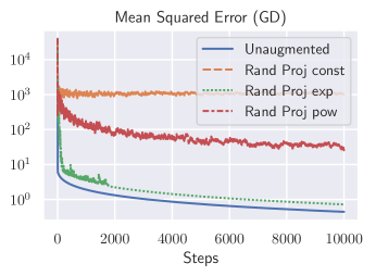
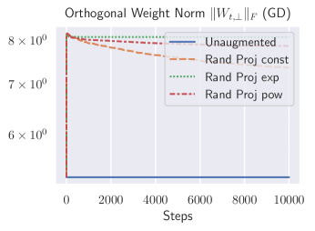
Figure E.1: MSE and $\|W_{t,\perp}\|_{F}$ for optimization trajectories of GD with random projection augmentation Jointly scheduling learning rate and noise variance to have polynomial decay is necessary for optimization to converge to the minimal norm solution $W_{\min}$. Rand Proj const, Rand Proj exp, and Rand Proj pow have random projection augmentation with $1-\gamma_{t}=0.1,0.1e^{-0.02t},0.1(1+\frac{t}{50})^{-0.33}$, respectively. Other experimental details are the same as those described in §E.3.

Appendix F Analysis of SGD

This section gives an analysis of vanilla SGD using our method. Let us briefly recall the notation. As before, we consider overparameterized linear regression with loss

$$\mathcal{L}(W;\mathcal{D})=\frac{1}{N}\left\|WX-Y\right\|_{F}^{2},$$

where the dataset $\mathcal{D}$ of size $N$ consists of data matrices $X,Y$ that each have $N$ columns $x_{i}\in\mathbb{R}^{n},y_{i}\in\mathbb{R}^{p}$ with $n>N.$ We optimize $\mathcal{L}(W;\mathcal{D})$ by augmented SGD either with or without additive Gaussian noise. In the former case, this means that at each time $t$ we replace $\mathcal{D}=(X,Y)$ by a random batch $\mathcal{B}_{t}=(X_{t},Y_{t})$ given by a prescribed batch size $B_{t}=|\mathcal{B}_{t}|$ in which each datapoint in $\mathcal{B}_{t}$ is chosen uniformly with replacement from $\mathcal{D}$, and the resulting data matrices $X_{t}$ and $Y_{t}$ are scaled so that $\overline{\mathcal{L}}_{t}(W)=\mathcal{L}(W;\mathcal{D})$. Concretely, this means that for the normalizing factor $c_{t}:=\sqrt{N/B_{t}}$ we have

$$X_{t}=c_{t}XA_{t}\qquad\text{and}\qquad Y_{t}=c_{t}YA_{t},$$ (F.1)

where $A_{t}\in\mathbb{R}^{N\times B_{t}}$ has i.i.d. columns $A_{t,i}$ with a single non-zero entry equal to $1$ chosen uniformly at random. In this setting the minimum norm optimum for each $t$ are the same and given by

$$W_{t}^{*}=W_{\min}=YX^{\mathsf{T}}(XX^{\mathsf{T}})^{+},$$

which coincides with the minimum norm optimum for the unaugmented loss.

Theorem F.1.

If the learning rate satisfies $\eta_{t}\to 0$ and

$$\sum_{t=0}^{\infty}\eta_{t}=\infty,$$ (F.2)

then for any initialization $W_{0}$, we have $W_{t}Q_{\parallel}\overset{p}{\to}W_{\min}$. If further we have that $\eta_{t}=\Theta(t^{-x})$ with $0<x<1$, then for some $C>0$ we have

$$e^{Ct^{1-x}}\|W_{t}Q_{\parallel}-W_{\min}\|_{F}\overset{p}{\to}0.$$

Theorem F.1 recovers the exponential convergence rate for SGD in the overparametrized settting, which has been previously studied through both empirical and theoretical means (ma2018power, ). Because $1\leq B_{t}\leq N$ for all $t$, it does not affect the asymptotic results in Theorem F.1. In practice, however, the number of optimization steps $t$ is often small enough that $\frac{B_{t}}{N}$ is of order $t^{-\alpha}$ for some $\alpha>0$, meaning the choice of $B_{t}$ can affect rates in this non-asymptotic regime. Though we do not attempt to push our generic analysis to this granularity, this is done in ma2018power to derive optimal batch sizes and learning rates in the overparametrized setting.

Proof of Theorem F.1.

In order to apply Theorems B.1 and B.4, we begin by computing the moments of $A_{t}$ as follows. Recall the notation $\operatorname{diag}(M)$ from Appendix A.1.

Lemma F.2.

For any $Z\in\mathbb{R}^{N\times N}$, we have that

$$\mathbb{E}[A_{t}A_{t}^{\mathsf{T}}]=\frac{B_{t}}{N}\operatorname{Id}_{N\times N}\qquad\text{and}\qquad\mathbb{E}[A_{t}A_{t}^{\mathsf{T}}ZA_{t}A_{t}^{\mathsf{T}}]=\frac{B_{t}}{N}\operatorname{diag}(Z)+\frac{B_{t}(B_{t}-1)}{N^{2}}Z.$$

Proof.

We have that

$$\mathbb{E}[A_{t}A_{t}^{\mathsf{T}}]=\sum_{i=1}^{B_{t}}\mathbb{E}[A_{i,t}A_{i,t}^{\mathsf{T}}]=\frac{B_{t}}{N}\operatorname{Id}_{N\times N}.$$

Similarly, we find that

$$\mathbb{E}[A_{t}A_{t}^{\mathsf{T}}ZA_{t}A_{t}^{\mathsf{T}}] =\sum_{i,j=1}^{B_{t}}\mathbb{E}[A_{i,t}A_{i,t}^{\mathsf{T}}ZA_{j,t}A_{j,t}^{\mathsf{T}}]$$

$$=\sum_{i=1}^{B_{t}}\mathbb{E}[A_{i,t}A_{i,t}^{\mathsf{T}}ZA_{i,t}A_{i,t}^{\mathsf{T}}]+2\sum_{1\leq i<j\leq B_{t}}\mathbb{E}[A_{i,t}A_{i,t}^{\mathsf{T}}ZA_{j,t}A_{j,t}^{\mathsf{T}}]$$

$$=\frac{B_{t}}{N}\operatorname{diag}(Z)+\frac{B_{t}(B_{t}-1)}{N^{2}}Z,$$

which completes the proof. ∎

Let us first check convergence in mean:

$$\mathbb{E}[W_{t}]Q_{\parallel}\to W_{\min}.$$

To see this, note that Lemma F.2 implies

$$\mathbb{E}[Y_{t}X_{t}^{\mathsf{T}}]=YX^{\mathsf{T}}\qquad\mathbb{E}[X_{t}X_{t}^{\mathsf{T}}]=XX^{\mathsf{T}},$$

which yields that

$$W_{t}^{*}=YX^{\mathsf{T}}[XX^{\mathsf{T}}]^{+}=W_{\min}$$ (F.3)

for all $t$. We now prove convergence. Since all $W_{t}^{*}$ are equal to $W_{\min}$, we find that $\Xi^{*}_{t}=0$. By (B.9) and Lemma F.2 we have

$$\mathbb{E}[W_{t+1}]-W_{\min}=(\mathbb{E}[W_{t}]-W_{\min})\Big{(}\operatorname{Id}-\frac{2\eta_{t}}{N}XX^{\mathsf{T}}\Big{)},$$

which implies since $\frac{2\eta_{t}}{N}<\lambda_{\text{max}}(XX^{\mathsf{T}})^{-1}$ for large $t$ that for some $C>0$ we have

$$\|\mathbb{E}[W_{t}]Q_{\parallel}-W_{\min}\|_{F}\leq\|W_{0}Q_{\parallel}-W_{\min}\|_{F}\prod_{s=0}^{t-1}\left\|Q_{\parallel}-\frac{2\eta_{s}}{N}XX^{\mathsf{T}}\right\|_{2}\\ \leq C\|W_{0}Q_{\parallel}-W_{\min}\|_{F}\exp\Big{(}-\sum_{s=0}^{t-1}\frac{2\eta_{s}}{N}\lambda_{\text{min},V_{\parallel}}(XX^{\mathsf{T}})\Big{)}.$$ (F.4)

From this we readily conclude using (F.2) the desired convergence in mean $\mathbb{E}[W_{t}]Q_{\parallel}\to W_{\min}$.

Let us now prove that the variance tends to zero. By Proposition B.6, we find that $Z_{t}=\mathbb{E}[(W_{t}-\mathbb{E}[W_{t}])^{\mathsf{T}}(W_{t}-\mathbb{E}[W_{t}])]$ has two-sided decay of type $(\{A_{t}\},\{C_{t}\})$ with

$$A_{t}=\frac{2\eta_{t}}{N}X_{t}X_{t}^{\mathsf{T}},\qquad C_{t}=\frac{4\eta_{t}^{2}}{N^{2}}\left[\operatorname{Id}\circ\text{Var}((\mathbb{E}[W_{t}]X_{t}-Y_{t})X_{t}^{\mathsf{T}})\right].$$

To understand the resulting rating of convergence, let us first obtain a bound on $\text{tr}(C_{t})$. To do this, note that for any matrix $A$, we have

$$\text{tr}\left(\operatorname{Id}\circ\text{Var}[A]\right)=\text{tr}\left(\mathbb{E}\left[A^{\mathsf{T}}A\right]-\mathbb{E}\left[A\right]^{\mathsf{T}}\mathbb{E}\left[A\right]\right).$$

Moreover, using the definition (F.1) of the matrix $A_{t}$ and writing

$$M_{t}:=\mathbb{E}\left[W_{t}\right]X-Y,$$

we find

$$\left((\mathbb{E}\left[W_{t}\right]X_{t}-Y_{t})X_{t}^{\mathsf{T}}\right)^{\mathsf{T}}(\mathbb{E}\left[W_{t}\right]X_{t}-Y_{t})X_{t}^{\mathsf{T}}=XA_{t}A_{t}^{\mathsf{T}}M_{t}^{\mathsf{T}}M_{t}A_{t}A_{t}^{\mathsf{T}}X^{\mathsf{T}}$$

as well as

$$\mathbb{E}\left[\left((\mathbb{E}[W_{t}]X_{t}-Y_{t})X_{t}^{\mathsf{T}}\right)\right]^{\mathsf{T}}\mathbb{E}\left[(\mathbb{E}[W_{t}]X_{t}-Y_{t})X_{t}^{\mathsf{T}}\right]=X\mathbb{E}\left[A_{t}A_{t}^{\mathsf{T}}\right]M_{t}^{\mathsf{T}}M_{t}\mathbb{E}\left[A_{t}A_{t}^{\mathsf{T}}\right]X^{\mathsf{T}}.$$

Hence, using the expression from Lemma F.2 for the moments of $A_{t}$ and recalling the scaling factor $c_{t}=(N/B_{t})^{1/2}$, we find

$$\text{tr}(C_{t})=\frac{4\eta_{t}^{2}}{B_{t}}\text{tr}\left(X\left\{\mathrm{diag}\left(M_{t}^{\mathsf{T}}M_{t}\right)-\frac{1}{N}M_{t}^{\mathsf{T}}M_{t}\right\}X^{\mathsf{T}}\right).$$

Next, writing

$$\Delta_{t}:=\mathbb{E}[W_{t}]-W_{\min}$$

and recalling (F.3), we see that

$$M_{t}=\Delta_{t}X.$$

Thus, applying the estimates (F.4) about exponential convergence of the mean, we obtain

$$\text{tr}(C_{t})\leq\frac{8\eta_{t}^{2}}{B_{t}}\left\|\Delta_{t}Q_{||}\right\|_{2}^{2}\left\|XX^{T}\right\|_{2}^{2}\leq C\frac{8\eta_{t}^{2}}{B_{t}}\left\|XX^{T}\right\|_{2}^{2}\|\Delta_{0}Q_{\parallel}\|_{F}^{2}\exp\Big{(}-\sum_{s=0}^{t-1}\frac{4\eta_{s}}{N}\lambda_{\text{min},V_{\parallel}}(XX^{\mathsf{T}})\Big{)}.$$ (F.5)

Notice now that $Y_{r}=Q_{\parallel}-A_{r}$ satisfies the conditions of Theorem A.6 with $a_{r}=1-2\eta_{r}\frac{1}{N}\lambda_{\text{min},V_{\parallel}}(XX^{\mathsf{T}})$ and $b_{r}^{2}=\frac{4\eta_{r}^{2}}{B_{r}a_{r}^{2}N}\text{tr}\Big{(}X\operatorname{diag}(X^{\mathsf{T}}X)X-\frac{1}{N}XX^{\mathsf{T}}XX^{\mathsf{T}}\Big{)}$. By Theorem A.6 we then obtain for any $t>s>0$ that

$$\mathbb{E}\left[\left\|\prod_{r=s+1}^{t}(Q_{\parallel}-A_{r})\right\|_{2}^{2}\right]\leq e^{\sum_{r=s+1}^{t}b_{r}^{2}}\prod_{r=s+1}^{t}\Big{(}1-2\eta_{r}\frac{1}{N}\lambda_{\text{min},V_{\parallel}}(XX^{\mathsf{T}})\Big{)}^{2}.$$ (F.6)

By two-sided decay of $Z_{t}$, we find by (F.5), (F.6), and (A.9) that

$$\mathbb{E}[\|W_{t}Q_{\parallel}-\mathbb{E}[W_{t}]Q_{\parallel}\|^{2}_{F}]=\text{tr}(Q_{\parallel}Z_{t}Q_{\parallel})\\ \leq e^{-\frac{4}{N}\lambda_{\text{min},V_{\parallel}}(XX^{\mathsf{T}})\sum_{s=0}^{t-1}\eta_{s}}\frac{\|XX^{\mathsf{T}}\|_{2}^{2}}{N^{2}}\|\Delta_{0}Q_{\parallel}\|_{F}^{2}C\sum_{s=0}^{t-1}\frac{8\eta_{s}^{2}}{B_{s}/N}e^{\frac{4\eta_{s}}{N}\lambda_{\text{min},V_{\parallel}}(XX^{\mathsf{T}})+\sum_{r=s+1}^{t}b_{r}^{2}}.$$ (F.7)

Since $\eta_{s}\to 0$, we find that $\eta_{s}\frac{N}{B_{s}}e^{\frac{4\eta_{s}}{N}\lambda_{\text{min},V_{\parallel}}(XX^{\mathsf{T}})}$ is uniformly bounded and that $b_{r}^{2}\leq\frac{4}{N}\lambda_{\text{min},V_{\parallel}}(XX^{\mathsf{T}})\eta_{r}$ for sufficiently large $r$. We therefore find that for some $C^{\prime}>0$,

$$\mathbb{E}[\|W_{t}Q_{\parallel}-\mathbb{E}[W_{t}]Q_{\parallel}\|_{F}^{2}]\leq C^{\prime}\sum_{s=0}^{t-1}\eta_{s}e^{-\frac{4}{N}\lambda_{\text{min},V_{\parallel}}(XX^{\mathsf{T}})\sum_{r=0}^{s}\eta_{r}},$$

hence $\lim_{t\to\infty}\mathbb{E}[\|W_{t}Q_{\parallel}-\mathbb{E}[W_{t}]Q_{\parallel}\|_{F}^{2}]=0$ by Lemma A.8. Combined with the fact that $\mathbb{E}[W_{t}]Q_{\parallel}\to W_{\min}$, this implies that $W_{t}Q_{\parallel}\overset{p}{\to}W_{\min}$.

To obtain a rate of convergence, observe that by (F.4) and the fact that $\eta_{t}=\Theta(t^{-x})$, for some $C_{1},C_{2}>0$ we have

$$\|\mathbb{E}[W_{t}]Q_{\parallel}-W_{\min}\|_{F}\leq C_{1}\exp\Big{(}-C_{2}t^{1-x}\Big{)}.$$ (F.8)

Similarly, by (F.7) and the fact that $\frac{\eta_{s}}{B_{s}/N}<\infty$ uniformly, for some $C_{3},C_{4},C_{5}>0$ we have

$$\mathbb{E}[\|W_{t}Q_{\parallel}-\mathbb{E}[W_{t}]Q_{\parallel}\|_{F}^{2}]\leq C_{3}\exp\Big{(}-C_{4}t^{1-x}\Big{)}t^{1-x}$$

We conclude by Chebyshev’s inequality that for any $a>0$ we have

$$\mathbb{P}\Big{(}\|W_{t}Q_{\parallel}-W_{\min}\|_{F}\geq C_{1}\exp\Big{(}-C_{2}t^{1-x}\Big{)}+a\cdot\sqrt{C_{3}}t^{\frac{1}{2}-\frac{x}{2}}e^{-C_{4}t^{1-x}/2}\Big{)}\leq a^{-2}.$$

Taking $a=t$, we conclude as desired that for some $C>0$, we have

$$e^{Ct^{1-x}}\|W_{t}Q_{\parallel}-W_{\min}\|_{F}\overset{p}{\to}0.$$

This completes the proof of Theorem F.1. ∎

References

- (1) F. Bach and E. Moulines. Non-strongly-convex smooth stochastic approximation with convergence rate . In Advances in neural information processing systems, pages 773–781, 2013.
- (2) P. L. Bartlett, P. M. Long, G. Lugosi, and A. Tsigler. Benign overfitting in linear regression. Proceedings of the National Academy of Sciences, 2020.
- (3) C. M. Bishop. Training with noise is equivalent to Tikhonov regularization. Neural computation, 7(1):108–116, 1995.
- (4) L. Bottou, F. E. Curtis, and J. Nocedal. Optimization methods for large-scale machine learning. Siam Review, 60(2):223–311, 2018.
- (5) O. Chapelle, J. Weston, L. Bottou, and V. Vapnik. Vicinal risk minimization. In T. K. Leen, T. G. Dietterich, and V. Tresp, editors, Advances in Neural Information Processing Systems 13, pages 416–422. MIT Press, 2001.
- (6) S. Chen, E. Dobriban, and J. H. Lee. Invariance reduces variance: Understanding data augmentation in deep learning and beyond. stat, 1050:25, 2019.
- (7) B. Collins and P. Śniady. Integration with respect to the Haar measure on unitary, orthogonal and symplectic group. Communications in Mathematical Physics, 264(3):773–795, Mar 2006.
- (8) E. D. Cubuk, B. Zoph, D. Mane, V. Vasudevan, and Q. V. Le. Autoaugment: Learning augmentation strategies from data. In Proceedings of the IEEE conference on computer vision and pattern recognition, pages 113–123, 2019.
- (9) E. D. Cubuk, B. Zoph, J. Shlens, and Q. V. Le. Randaugment: Practical automated data augmentation with a reduced search space. In Proceedings of the IEEE/CVF Conference on Computer Vision and Pattern Recognition Workshops, pages 702–703, 2020.
- (10) T. Dao, A. Gu, A. Ratner, V. Smith, C. De Sa, and C. Re. A kernel theory of modern data augmentation. volume 97 of Proceedings of Machine Learning Research, pages 1528–1537, Long Beach, California, USA, 09–15 Jun 2019. PMLR.
- (11) A. Défossez and F. Bach. Averaged least-mean-squares: Bias-variance trade-offs and optimal sampling distributions. In Artificial Intelligence and Statistics, pages 205–213, 2015.
- (12) T. DeVries and G. W. Taylor. Improved regularization of convolutional neural networks with cutout. arXiv preprint arXiv:1708.04552, 2017.
- (13) P. Goyal, P. Dollár, R. Girshick, P. Noordhuis, L. Wesolowski, A. Kyrola, A. Tulloch, Y. Jia, and K. He. Accurate, large minibatch SGD: Training Imagenet in 1 hour. arXiv preprint arXiv:1706.02677, 2017.
- (14) Y. Grandvalet and S. Canu. Noise injection for inputs relevance determination. In Advances in intelligent systems, pages 378–382. IOS Press, 1997.
- (15) S. Gunasekar, J. Lee, D. Soudry, and N. Srebro. Characterizing implicit bias in terms of optimization geometry, 2020.
- (16) D. Hendrycks, N. Mu, E. D. Cubuk, B. Zoph, J. Gilmer, and B. Lakshminarayanan. AugMix: A simple data processing method to improve robustness and uncertainty. Proceedings of the International Conference on Learning Representations (ICLR), 2020.
- (17) D. Ho, E. Liang, X. Chen, I. Stoica, and P. Abbeel. Population based augmentation: Efficient learning of augmentation policy schedules. In International Conference on Machine Learning, pages 2731–2741, 2019.
- (18) D. Huang, J. Niles-Weed, J. A. Tropp, and R. Ward. Matrix concentration for products, 2020.
- (19) D. LeJeune, R. Balestriero, H. Javadi, and R. G. Baraniuk. Implicit rugosity regularization via data augmentation. arXiv preprint arXiv:1905.11639, 2019.
- (20) A. Lewkowycz and G. Gur-Ari. On the training dynamics of deep networks with regularization. arXiv preprint arXiv:2006.08643, 2020.
- (21) F. Liu, A. Najmi, and M. Sundararajan. The penalty imposed by ablated data augmentation. arXiv preprint arXiv:2006.04769, 2020.
- (22) S. Ma, R. Bassily, and M. Belkin. The power of interpolation: Understanding the effectiveness of SGD in modern over-parametrized learning. In International Conference on Machine Learning, pages 3325–3334. PMLR, 2018.
- (23) D. S. Park, W. Chan, Y. Zhang, C.-C. Chiu, B. Zoph, E. D. Cubuk, and Q. V. Le. SpecAugment: A simple data augmentation method for automatic speech recognition. Proc. Interspeech 2019, pages 2613–2617, 2019.
- (24) S. Rajput, Z. Feng, Z. Charles, P.-L. Loh, and D. Papailiopoulos. Does data augmentation lead to positive margin? arXiv preprint arXiv:1905.03177, 2019.
- (25) H. Robbins and S. Monro. A stochastic approximation method. Ann. Math. Statist., 22(3):400–407, 09 1951.
- (26) P. Simard, D. Steinkraus, and J. Platt. Best practices for convolutional neural networks applied to visual document analysis. In Seventh International Conference on Document Analysis and Recognition, 2003. Proceedings., volume 2, pages 958–958, 2003.
- (27) S. L. Smith, P.-J. Kindermans, C. Ying, and Q. V. Le. Don’t decay the learning rate, increase the batch size. In International Conference on Learning Representations, 2018.
- (28) S. L. Smith and Q. V. Le. A Bayesian perspective on generalization and stochastic gradient descent. In International Conference on Learning Representations, 2018.
- (29) D. Soudry, E. Hoffer, M. S. Nacson, S. Gunasekar, and N. Srebro. The implicit bias of gradient descent on separable data, 2018.
- (30) S. Wager, S. Wang, and P. S. Liang. Dropout training as adaptive regularization. In Advances in neural information processing systems, pages 351–359, 2013.
- (31) D. Wu and J. Xu. On the optimal weighted regularization in overparameterized linear regression. arXiv preprint arXiv:2006.05800, 2020.
- (32) J. Wu, D. Zou, V. Braverman, and Q. Gu. Direction matters: On the implicit bias of stochastic gradient descent with moderate learning rate, 2021.
- (33) L. Wu, C. Ma, and E. Weinan. How SGD selects the global minima in over-parameterized learning: A dynamical stability perspective. In Advances in Neural Information Processing Systems, pages 8279–8288, 2018.
- (34) S. Wu, H. R. Zhang, G. Valiant, and C. Ré. On the generalization effects of linear transformations in data augmentation, 2020.
- (35) H. Zhang, M. Cisse, Y. N. Dauphin, and D. Lopez-Paz. mixup: Beyond empirical risk minimization. arXiv preprint arXiv:1710.09412, 2017.