Tropospheric Composition and Circulation of Uranus with ALMA and the VLA

Abstract

We present ALMA and VLA spatial maps of the Uranian atmosphere taken between 2015 and 2018 at wavelengths from 1.3 mm to 10 cm, probing pressures from $\sim$1 to $\sim$50 bar at spatial resolutions from 0.1” to 0.8”. Radiative transfer modeling was performed to determine the physical origin of the brightness variations across Uranus’s disk. The radio-dark equator and midlatitudes of the planet (south of $\sim$50^∘ N) are well fit by a deep H₂S mixing ratio of $8.7_{-1.5}^{+3.1}\times 10^{-4}$ ($37_{-6}^{+13}\times$ Solar) and a deep NH₃ mixing ratio of $1.7_{-0.4}^{+0.7}\times 10^{-4}$ ($1.4_{-0.3}^{+0.5}\times$ Solar), in good agreement with literature models of Uranus’s disk-averaged spectrum. The north polar region is very bright at all frequencies northward of $\sim$50^∘N, which we attribute to strong depletions extending down to the NH₄SH layer in both NH₃ and H₂S relative to the equatorial region; the model is consistent with an NH₃ abundance of $4.7_{-1.8}^{+2.1}\times 10^{-7}$ and an H₂S abundance of $<$$1.9\times 10^{-7}$ between $\sim$20 and $\sim$50 bar. Combining this observed depletion in condensible molecules with methane-sensitive near-infrared observations from the literature suggests large-scale downwelling in the north polar vortex region from $\sim$0.1 to $\sim$50 bar. The highest-resolution maps reveal zonal radio-dark and radio-bright bands at 20^∘S, 0^∘, and 20^∘N, as well as zonal banding within the north polar region. The difference in brightness is a factor of $\sim$10 less pronounced in these bands than the difference between the north pole and equator, and additional observations are required to determine the temperature, composition and vertical extent of these features.

1 Introduction

Uranus’s 82^∘ obliquity leads to drastic seasonal variations in insolation, with both poles receiving more annual sunlight than the equator. In addition, Uranus is the only giant planet that lacks an apparent internal heat source (Pearl et al., 1990). The unusual pattern of heat flux into the Uranian troposphere resulting from these two characteristics provides an extreme test of our understanding of atmospheric circulation (for recent reviews see Hueso & Sánchez-Lavega, 2019; Fletcher et al., 2020). The strong seasonal forcing also plays a role in altering Uranus’s atmospheric composition; for example, Uranus’s insolation pattern has been invoked to explain the disequilibrium in the H₂ ortho-para fraction in the upper troposphere as well as the seasonal variation in haze properties and/or methane abundance in the stratosphere (Hueso & Sánchez-Lavega, 2019). Radio observations provide a unique tool for probing the atmosphere of Uranus beneath its tropospheric cloud layers, permitting inferences about its tropospheric properties (Jaffe et al., 1984; de Pater & Gulkis, 1988; Hofstadter & Muhleman, 1989; Hofstadter et al., 1990; de Pater et al., 1991; Hofstadter, 1992; Hofstadter & Butler, 2003; Klein & Hofstadter, 2006).

Central to these questions is Uranus’s global circulation pattern. Remote-sensing observations probe atmospheric vertical motions indirectly by determining the zonal-mean distribution of condensible gases and clouds. Regions of large-scale upwelling are cloudy and rich in condensible gases up to the condensation pressure of that gas, while downwelling regions are drier and less cloudy. This point can be understood by analogy to the Hadley cell on Earth (see, e.g., Marshall & Plumb, 1989). Water vapor evaporated from the deep reservoir (the ocean) moves equatorward into the Intertropical Convergence Zone (ITCZ), where it upwells, condenses as the tropospheric temperature decreases with altitude, and then rains back into the deep reservoir. The air leaving the top of the ITCZ has thus been robbed of its water vapor by the tropopause cold trap, so the divergent upper branch and subsiding sub-tropical branch of the circulation cell are much drier than the ITCZ both in terms of relative humidity and column-integrated water vapor. The atmospheres of the giant planets organize into a series of alternating thermally direct and thermally indirect circulation cells similar to Earth’s Hadley and Ferrel cells, giving rise to the spectacular jets of Jupiter and Saturn. Global circulation models (GCMs) of Jupiter show that the zonal-mean column-integrated abundances of both ammonia and water are indeed higher in the upwelling branches and lower in the downwelling branches (Young et al., 2019a, b), in agreement with ground-based (e.g., de Pater et al., 2016, 2019) and spacecraft (Li et al., 2017) data. Based on Voyager thermal-infrared measurements, Flasar et al. (1987) suggested a circulation model for Uranus with gas rising at latitudes near 30^∘ and subsiding at the equator and poles. Observations with the Very Large Array (VLA) revealed a bright south pole on Uranus, interpreted as a relative lack of microwave opacity in the deep troposphere down to $\sim$50 bar, which pointed to large-scale subsidence of dry air (Jaffe et al., 1984; de Pater & Gulkis, 1988; de Pater et al., 1989; Hofstadter et al., 1990; de Pater et al., 1991; Hofstadter, 1992; Hofstadter & Butler, 2003; Klein & Hofstadter, 2006). A polar depletion in both methane and hydrogen sulfide (H₂S) at higher altitudes observed at visible and near-infrared wavelengths corroborated this interpretation (Karkoschka & Tomasko, 2009; Sromovsky et al., 2014; Irwin et al., 2018; Sromovsky et al., 2019). Together, these multi-wavelength observations lent further support to the Flasar et al. (1987) non-seasonal equator-to-pole single-cell meridional circulation pattern (de Pater et al., 1991; Hofstadter, 1992; Sromovsky et al., 2014). However, a single-celled model has difficulty explaining the observed bands of clouds at 38^∘ and 58^∘ in both hemispheres. An alternative model prescribing circulation in three vertically stacked layers was proposed by Sromovsky et al. (2014), although those authors make clear that the three-layer model has shortcomings of its own. It also remains unclear how the bright storm systems observed occasionally at near-infrared wavelengths, which appear to migrate in latitude (Sromovsky et al., 2007; de Pater et al., 2011, 2015), fit into either model.

Previously published radio and millimeter observations of Uranus (e.g. Jaffe et al., 1984; de Pater & Gulkis, 1988), mostly taken prior to 1990, have mostly considered the disk-integrated planet and primarily imaged Uranus’s southern hemisphere. More recent spatially resolved observations using the VLA have been presented at conferences (e.g., Hofstadter et al., 2009) and featured in a recent white paper (de Pater et al., 2018). Both the Hofstadter et al. (2009) image from 2005 and the de Pater et al. (2018) image from 2015, which is analyzed in detail in this paper, show alternating bright and dark zonal bands in the midlatitudes, indicating a more complex circulation pattern than current models. The bright polar regions display similar brightness temperatures and zonal extents in the 2005 image, in which both poles are visible, and in the 2015 image zonal banding is visible within the bright polar region.

Inferences about the vertical cloud structure of giant planets are made by comparing radiative transfer and chemical modeling to observational data across the electromagnetic spectrum. Visible and near-infrared spectroscopy (e.g., Karkoschka & Tomasko, 2009; Tice et al., 2013; Sromovsky et al., 2014; de Kleer et al., 2015; Sromovsky et al., 2019) have identified methane as the major condensible species in the upper troposphere, producing bright clouds and weather readily observed in visible/IR imaging (e.g., de Pater et al., 2011, 2015; Sromovsky et al., 2015). At $\sim$35 bar, gaseous NH₃ and H₂S are expected to precipitate into a cloud of solid NH₄SH, effectively removing either all nitrogen or all sulfur from the upper atmosphere. Gulkis et al. (1978) showed that Uranus must be ammonia-poor above the NH₄SH layer in order to fit the planet’s disk-integrated radio spectrum. This finding suggested, contrary to solar composition models, that more H₂S than NH₃ was present in Uranus’s deep atmosphere. Further work indicated that H₂S itself was also a major absorber, and new models, still with more sulfur than nitrogen, were developed that improved the fit to the observed spectra (de Pater et al., 1991; de Pater, 2018). Based on these studies, the uniform cloud layer at $\sim$3 bar, evident in IR spectroscopy, was long assumed to be composed of H₂S ice particles; this hypothesis was confirmed recently by the direct detection of H₂S spectral lines above the cloud (Irwin et al., 2018). The chemistry becomes more speculative at pressures deeper than $\sim$50 bars, as those depths have not been accessed observationally. Models suggest Uranus’s oxygen is locked in a water-ice cloud at $\sim$270 K ($\sim$50 bar), and beneath this, an aqueous nitrogen-, sulfur-, and oxygen-bearing solution is expected to form (Weidenschilling & Lewis, 1973; Atreya & Romani, 1985). The effects of phosphine (PH₃) have also been considered in the ice giants. Its condensation pressure is near 80 K ($\sim$1 bar on Uranus), and modeling shows that its absorption at deeper layers may be important to Uranus’s infrared and millimeter spectrum (e.g., Fegley & Prinn, 1986; Hoffman et al., 2001), especially near its $J=1\rightarrow 0$ rotational transition at 1.123 mm (266.9 GHz). However, its presence has never been confirmed observationally (Orton & Kaminski, 1989; Moreno et al., 2009).

In this paper we present new VLA and ALMA observations of Uranus’s atmosphere from 2015 to 2018, representing the highest sensitivity and spatial resolution measurements of the planet at wavelengths from 1.3 mm to 10 cm. In Section 2 we outline the observational techniques and data processing procedures used to produce science images of Uranus. We present our results in Section 3, including seasonal brightness trends, spatial variations in brightness temperature, and inferred properties of Uranus’s troposphere as determined from radiative transfer modeling. Finally, we put our results in a broader context and provide concluding remarks in Section 4.

2 Observations and Data Reduction

We obtained observations of Uranus with the Karl G. Jansky Very Large Array (VLA) from 0.9-10 cm (3.0-33 GHz) in August 2015 and the Atacama Large (sub-)Millimeter Array (ALMA) from 1.3-3.1 mm (98-233 GHz) between December 2017 and September 2018. A table of observations is provided in Table 1. The data-reduction procedures are outlined in the following two subsections.

	Wavelength	Frequency		On-Source	Resolution	Resolution	Flux & Gain	Phase	Sub-Obs
Array	(mm)	(GHz)	UT Date	Time (min)	(arcsec)	(km)	Calibrator	Calibrator	Latitude (∘)
VLA	95	3.2	2015-08-29	88	0.79	11000	3C48	J0121+422	33
VLA	51	5.8	2015-08-29	89	0.45	6300	3C48	J0121+422	33
VLA	30.	9.9	2015-08-29/30	150	0.26	3600	3C48	J0121+422	33
VLA	20.	15	2015-08-29/30	148	0.17	2400	3C48	J0121+422	33
VLA	9.1	33	2015-08-29/30	160	0.085	1200	3C48	J0121+422	33
ALMA	3.1	98	2017-12-03	42	0.19	2700	J0238+1636	J0121+1149	38
ALMA	3.1	98	2017-12-06	42	0.19	2700	J0238+1636	J0121+1149	38
ALMA	2.1	144	2017-12-27	22	0.21	3000	J0238+1636	J0121+1149	38
ALMA	1.3	233	2018-09-13	24	0.29	4000	J0237+2848	J0211+1051	45

Table 1: Table of observations. Note that the VLA observations at 0.9 cm, 2 cm, and 3 cm were taken in two parts over two consecutive days.

2.1 ALMA Data

The data in each of the three ALMA bands were flagged and calibrated by the North American ALMA Science Center using the standard data-reduction procedures contained in the NRAO’s CASA software version 5.1.1. Standard flux- and phase-calibration procedures were carried out by applying the pipeline using the quasars listed in Table 1 as calibrator sources. The CASA pipeline retrieved flux calibration errors of $\sim$5% in all three bands. Iterative phase-only self-calibration, which is routinely applied to radio observations of bright planets (e.g., Butler et al., 2001; de Pater et al., 2014, 2019), was performed using a procedure similar to that outlined in Brogan et al. (2018) using solution intervals of 20, 10, 5, and 1 minutes in that order. To reduce ringing in the image plane from the presence of the bright planet, a uniform limb-darkened disk model of Uranus was subtracted from the data in the UV plane in each band, as done in, e.g., de Pater et al. (2014, 2016). The disk-subtracted data were inverted into the image plane and deconvolved using CASA’s tclean function. The resulting disk-subtracted images are shown in Figure 1. These images are also shown cylindrically projected onto a latitude-longitude grid in Figure 2. It should be noted that the planet’s rotation smears out features in longitude: the $\sim$20 minute observations at 2.1 mm and 1.3 mm are smeared by $\sim$8^∘, and the 3.1 mm image is a sum of two $\sim$40 minute observations taken at different sub-observer longitudes.

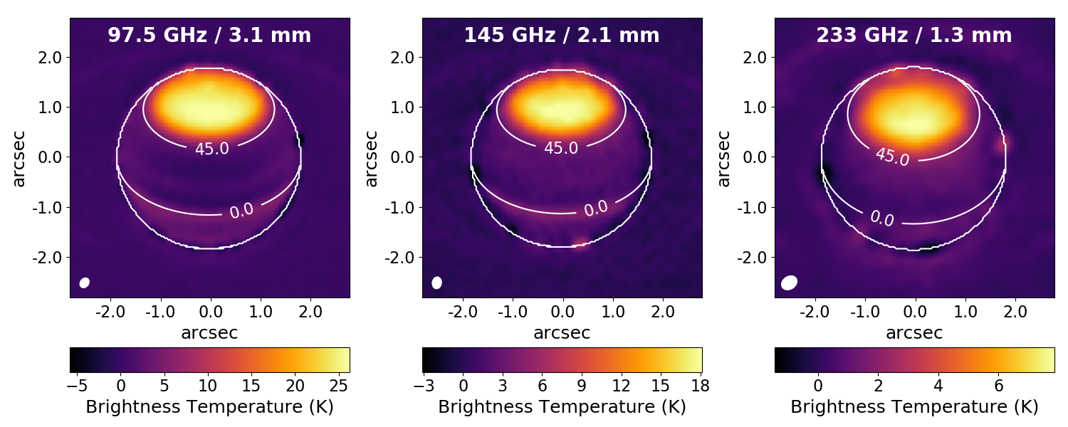
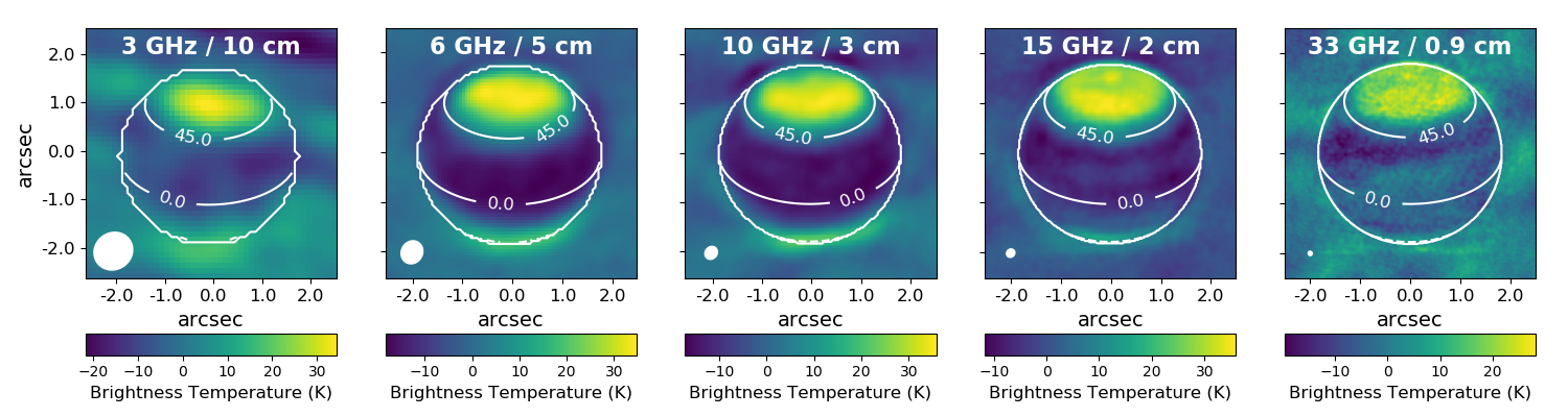
Figure 1: Disk-subtracted images of Uranus from ALMA (top) at 3.1 mm (Band 3), 2.1 mm (Band 4), and 1.3 mm (Band 6), and the VLA (bottom) from 0.9-20 cm. The color bars below each image indicate the brightness temperature residuals in Kelvin. The synthesized beam is shown as a white ellipse in the bottom left corner of each image. The ring of light and dark one-beam-size spots around the planet are artefacts produced by applying a Fourier transform to the UV-plane data near the sharp edges of the bright planet.

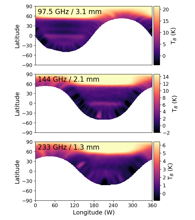
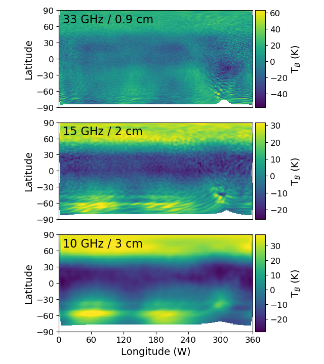
Figure 2: Left: Reprojected ALMA maps of Uranus. The $\sim$20 minute observations at 2.1 mm and 1.3 mm are smeared by $\sim$8^∘, and the 3.1 mm image is a sum of two $\sim$40 minute observations taken at different sub-observer longitudes. The alternating bright and dark spots near the planet’s limb are due to CLEAN artefacts, induced by attempting to Fourier transform a sharp-edged planet and made larger in apparent size by projection effects. Right: Longitude-resolved VLA maps of Uranus, produced using the faceting technique (Sault et al., 2004). The distortions near 300^∘W are due to poor zonal coverage at those longitudes in the observations. The spatial resolution of the 5 cm and 10 cm data is not sufficient to produce reliable longitude-resolved maps, so these are not shown.

Images were also produced from the calibrated but non-disk-subtracted data; these images were used to measure absolute fluxes across the disk for radiative transfer modeling. The $\sim$3.5” disk of Uranus was smaller than the maximum recoverable scale of the ALMA array configuration in all three observing bands; therefore we have short enough baselines to faithfully measure Uranus’s total flux. These flux measurements were confirmed by fitting the visibility data to a Bessel function; the difference between the UV-plane-derived and image-plane-derived total flux measurements was much smaller than the flux calibration error at all wavelengths. The total flux measurements were corrected for the cosmic microwave background (CMB) according to the prescription detailed in Appendix A of de Pater et al. (2014). Final measurements of Uranus’s disk-averaged brightness temperature are plotted against measurements from the literature in Figure 3 and tabulated in Table 2.

Figure 3: Disk-integrated brightness temperatures of Uranus from this work (red points) compared to measurements from the literature (black points; Gulkis & de Pater, 1984; Orton et al., 1986; de Pater & Gulkis, 1988; Muhleman & Berge, 1991; Griffin & Orton, 1993). As shown by those authors (see also Figure 4), the scatter in the data is primarily due to real seasonal fluctuations in Uranus’s observed brightness temperature as the planet’s poles move into and out of view. Our data fall at a lower brightness temperature than the majority of the literature data because those were observed in southern summer, when the bright south polar region made up a large fraction of Uranus’s disk. A radiative transfer model with parameters retrieved to match our 25^∘N data (Section 3.3), shown by a blue line, matches the disk-averaged data quite well.

Wavelength	Frequency	Disk-averaged	25∘ N	75∘ N	Flux Cal	RMS per	Latitude Bin
(mm)	(GHz)	$T_{B}$ (K)	$T_{B}$ (K)	$T_{B}$ (K)	Error (K)	Beam (K)	Error (K)
95	3.2	251.3	261.3	293.4	7.5	2.2	3.6
51	5.8	219.3	219.2	262.0	6.6	0.8	2.6
30.	9.9	184.5	182.8	224.4	5.5	1.2	2.6
20.	15	173.9	169.4	205.0	5.2	1.3	2.6
9.1	33	152.4	157.8	180.6	10.7	3.4	2.6
3.1	98	140.7	142.6	165.1	7.0	0.3	1.1
2.1	144	122.5	126.5	139.1	6.6	0.1	0.9
1.3	233	91.1	96.0	101.8	4.8	0.1	0.5

Table 2: Brightness temperature measurements and errors extracted from the ALMA and VLA maps. See Section 2 for discussion of the flux calibration and per-bin RMS errors, and Section 3.2 for discussion of the latitude-bin error.

2.2 VLA Data

The data in each of the five VLA bands were flagged and calibrated using the standard data-reduction procedures contained in the MIRIAD software package (Sault et al., 1995). Standard flux- and phase-calibration procedures were carried out using the calibrator sources listed in Table 1; the absolute flux calibration error was assumed to be 3% at the longest four wavelengths and 7% at 0.9 cm (Butler et al., 2001; Perley & Butler, 2013, 2017). Iterative self-calibration, disk subtraction, imaging, and deconvolution were carried out in a similar manner to the ALMA data but using MIRIAD. The CMB correction was applied in the same way as for the ALMA images. The resulting disk-subtracted images are shown in Figure 1. It should be noted that the 0.9 cm images are more strongly affected by imaging artefacts than the other bands because this wavelength sits near a telluric water absorption band, leading to relatively poor phase stability. Longitude-resolved images, produced using the faceting technique developed and recently used for VLA observations of Jupiter (Sault et al., 2004; de Pater et al., 2019), are shown in Figure 2. This represents the first attempt to resolve Uranus in longitude at these wavelengths. Limited UV-plane coverage leads to significant artefacts in these maps, including large-scale alternating bright and dark regions (e.g., bright at 60^∘W and 200^∘W in the 2 cm and 3 cm images) that cross many latitude bands. An apparent warping near 300^∘W is also present, caused by poor zonal coverage at those longitudes. Nevertheless, if any vortex-like disturbances at the scale of Jupiter’s Great Red Spot were present on Uranus, these maps should have detected them. No such structures are found, so in this work we focus our analysis on the longitude-smeared maps only.

3 Results and Discussion

3.1 Seasonal Brightness Variations

We explore long-term trends in Uranus’s radio brightness in Figure 4, which plots our VLA 3.0 cm data along with 3.5 cm data obtained by Klein & Hofstadter (2006) and older disk-averaged data from various telescopes (Gulkis & de Pater, 1984) as a function of sub-observer latitude. Our data were taken with Uranus’s north pole facing the observer, whereas the Klein & Hofstadter (2006) data were taken toward the south pole; nevertheless, Uranus’s brightness temperature was the same within the error bars of the data at a sub-observer longitude of $\sim$35^∘. The $\sim$40 K brightness difference we observe between Uranus’s northern midlatitudes and its north pole at 2-3 cm is of the same magnitude as VLA measurements of the difference between the south polar region and southern midlatitudes (e.g., Hofstadter et al., 1990). Imaging at 1.3 cm taken near equinox (observers Hofstadter & Butler; de Pater et al., 2018), which appears to show that both poles are roughly equally bright, further supports the similarity in brightness temperature between the north and south pole. Any trend in the 3 mm brightness temperature (right panel of Figure 4) is much less clear; the error bars are large for all observations taken near equinox, and all data taken at sub-observer latitudes larger than 40^∘ have the same brightness to within the 2$\sigma$ level. This is confusing given the very large and bright north polar region we observe and the clear brightness temperature variations at longer wavelengths. However, the flux calibration uncertainty from measurements in some older papers (see references in Gulkis & de Pater, 1984) have not been reported and so this result should be treated with caution.

Figure 4: Left: VLA 3.0 cm total flux measurement of Uranus’s disk from this work (red) compared to 3.5 cm flux measurements made with the Goldstone station of NASA’s Deep Space Network (DSN) at a range of sub-observer latitudes (Klein & Hofstadter, 2006), as well as 3.5 cm measurements made prior to 1984 as summarized in Gulkis & de Pater (1984). Right: ALMA 3.1 mm total flux measurement of Uranus’s disk from this work (red) compared to previous mm-wavelength measurements from various authors (Gulkis & de Pater, 1984; Orton et al., 1986; Muhleman & Berge, 1991). The error bars on the literature measurements in both panels should be treated with caution, as flux calibration errors are often not reported. For the purposes of this plot we have added 5% flux calibration errors to the points from the Gulkis and Muhleman papers. The x-axis in both panels shows the absolute value of sub-observer latitude; note that all previous measurements were made at negative sub-observer latitudes.

3.2 Spatially Resolved Brightness Temperatures

The images in Figures 1 and 2 reveal complex banding structure in Uranus’s troposphere. For better visual comparison of the zonal features in the maps at different frequencies, a vertical slice of width 30^∘ longitude centered on the sub-observer point was taken from the longitude-smeared, disk-subtracted, projected maps (shown in Figure 2 for the ALMA data) at each frequency, then averaged into a 1-D brightness versus latitude profile. The resulting profiles are shown normalized relative to one another in Figure 5. To extract spatially-resolved brightness temperatures for radiative transfer modeling, we simply averaged non-disk-subtracted latitude profiles over ten degrees latitude; that is, the 25^∘N region represents latitudes from 20-30^∘N and the 75^∘N region represents latitudes from 70-80^∘N. The error on the extracted brightness temperatures was determined by making latitude profiles over several different 30^∘ longitude ranges and computing the standard deviation in the brightness measurements from those profiles. These “latitude-bin” errors are given in Table 2. It is worth noting that they are larger than the per-beam RMS error extracted from background regions of the radio maps (except at 0.9 cm). This is due to systematic errors arising from inverting and CLEANing visibility data of a very bright, extended, and sharp-edged source.

Figure 5: Meridional brightness profiles of the zonally-averaged radio/millimeter maps. Left: The 3.1 mm ALMA and 2.0 cm VLA data are plotted separately because they provide the best combination of high signal-to-noise ratio and resolution. These are compared to the brightness ratio between the Keck PaBeta (1.29 $\mu$m) and He1A (1.08 $\mu$m) filters, which is a tracer of the upper tropospheric methane abundance, as derived from 2015 imaging (Sromovsky et al., 2019, ; black dashed line). The PaBeta/He1A ratio curve and VLA 2 cm curve have been convolved with a 1-D Gaussian beam at the ALMA 3.1 mm resolution (0.19 arcsec); the $\sim$6^∘ FWHM of the beam at the sub-observer point is shown in the bottom right corner. Right: Latitudinal brightness profiles at all the observed wavelengths are plotted against one another. The FWHM of the beam at the sub-observer point is shown for representative frequencies in the same color as the data for that frequency. To facilitate visual comparison, the brightness temperature units in both panels are normalized so each band has maximum one.

The north polar region is readily observed across the radio and millimeter spectrum as a prominent brightening northward of $\sim$50^∘N. At 3.1 mm wavelength, this brightening reaches $>$25 K, nearly ten times the magnitude of any other brightness variations observed across Uranus’s disk. The edge of this brightening appears sharply defined: the transition from the darker midlatitudes to the bright poles occurs over less than a single resolution element in all the observing bands. The magnitude of the polar brightening is much too large to be explained by variations in kinetic temperature (see Appendix A), so we attribute it to downwelling air dry in absorbing species such as NH₃ and H₂S. Keck observations in the methane-sensitive PaBeta and H₂-sensitive He1A filters in 2015 (Sromovsky et al., 2019, simultaneous with our VLA observations) revealed a strong polar methane depletion that is spatially correlated with the bright polar region observed in the millimeter and radio data (see Figure 5). This implies continuously downwelling dry air over a wide range of pressures from 0.1 to at least 20 bar (see Section 3.3) at latitudes northward of 50^∘N. However, localized regions of upwelling (i.e. convection) or a temporally variable circulation pattern at the north pole cannot be ruled out. At 0.9 cm and 2 cm wavelengths, the highest-resolution VLA bands, a polar collar is observed at $\sim$60^∘N, just north of the 45^∘ polar collar seen at near-infrared wavelengths (see also Figure 5) but at the same latitude as the transition to solid-body rotation in Uranus’s zonal wind profile (Sromovsky et al., 2012). The polar collar is bounded by a somewhat fainter band at $\sim$75^∘N, then another brightening right at the north pole. However, this banding is not observed in the ALMA data despite similar spatial resolutions in the 3 mm and 2 cm data.

Alternating bright and dark bands are observed near Uranus’s equator in some of our images, with brighter latitudes at $\sim$20^∘S, $\sim$0^∘, and $\sim$20^∘N. At 3.1 mm, these bands are $\sim$1 K, $\sim$4 K, and $\sim$1 K brighter, respectively, than their surroundings. The banding is visible in all the ALMA data (3.1 mm, 2.1 mm, and 1.3 mm). It is also observed faintly in the 2 cm and 0.9 cm VLA bands, but not at longer wavelengths. Using our radiative transfer model (see Section 3.3), we find that variations in the CH₄ abundance, the PH₃ abundance, the relative humidity of H₂S, or the ortho-para fraction can all produce stronger absorption from 1 to 3 mm than at wavelengths longer than 2 cm. Changes in the kinetic temperature may also be responsible for all or part of the brightness temperature banding; however, this would require unusual atmospheric temperature profiles to fit our radio-millimeter spectrum (see Appendix A for a discussion of the kinetic temperature as it relates to the polar region). These putative abundance variations suggest downwelling and depletion in condensing species at the brighter latitudes extending at least from $\sim$1 to 5 bar. The lack of strong banding at longer wavelengths means that either the depletions do not extend deeper than 5-10 bar, the depletions are caused by a species that absorbs more strongly at shorter wavelengths, or the longer-wavelength VLA observations lack the sensitivity and spatial resolution to detect these faint equatorial bands. These observations point to a more complex circulation pattern than predicted by models (Flasar et al., 1987; Allison et al., 1991; Sromovsky et al., 2014), which suggested upwelling near 30^∘N and 30^∘S and subsidence at the equator and poles. A recent review paper (Fletcher et al., 2020) considered a more complex model that prescribes tropospheric upwelling at the equator and just equatorward of the polar region ($\sim$40^∘N), and downwelling between these. This model captures the large region of subsidence that we require at the poles. However, the alternating bright and dark bands we see, if indeed tied to upwelling and downwelling, do not match very well the locations prescribed in their model.

3.3 Radiative Transfer Modeling

The combined ALMA and VLA datasets comprise a spectrum of Uranus. Here we use radiative transfer models to fit this spectrum and infer the vertical distribution of condensible species in Uranus’s atmosphere. Radiative transfer modeling was carried out using the radio-BEAR (radio-BErkeley Atmospheric Radiative transfer) code. The cloud model and radiative transfer scheme are described in detail in de Pater et al. (2005, 2014, 2019). Radio-BEAR assumes that the atmosphere is in local thermodynamic equilibrium; its temperature follows an adiabat with a temperature of 76.4 K at 1 bar as determined by radio-occultation experiments with Voyager 2 (Lindal et al., 1987). At higher altitudes, where radiative effects become important, we used the temperature-pressure profile derived from Voyager/IRIS observations by Orton et al. (2015). The temperature-pressure profile is shown in Figure 6. Cloud densities may affect the millimeter and/or radio spectrum via absorption and scattering; however, too little is known about the cloud properties on Uranus to make an accurate cloud density model and clouds have been shown not to significantly affect the opacity at these wavelengths on Jupiter (de Pater et al., 2019). RadioBEAR therefore ignores cloud opacity and considers only gas absorption.

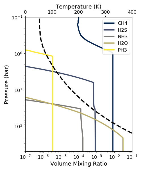
Figure 6: Vertical abundance profiles for trace gases in our radiative transfer model. Deep atmospheric abundances are set to 35$\times$ Solar except for NH₃, which has an abundance of 1$\times$ Solar. The dashed black line plots the assumed temperature-pressure profile, which follows a moist adiabat.

We started with a nominal disk-averaged model that assumed deep H₂S, H₂O, and CH₄ abundances of 30$\times$ Solar and a deep NH₃ abundance of 1$\times$ Solar (de Pater et al., 1991, 2018). The vertical profiles of these gases were determined using a cloud-physics model (Atreya & Romani, 1985; Romani, 1986; de Pater et al., 1991) that includes prescriptions for a water-solution cloud at $\gtrsim$100 bar and an NH₄SH layer at $\sim$35 bar. We added in PH₃ with a nominal deep abundance of 30$\times$ Solar and a simple prescription for its saturation vapor curve (Orton & Kaminski, 1989). Vertical profiles of all the condensible gases included in the radiative transfer code are plotted in Figure 6. The observed frequencies are sensitive to the atmospheric abundance and temperature from $\sim$0.1-50 bar; contribution functions at each frequency for the nominal model are shown in Figure 7.

We next perturbed many possible variables within this model one at a time to observe their effect on the spectrum, namely: the abundances of NH₃, H₂S, CH₄, and PH₃ from 500 bar up to just below the NH₄SH layer; the relative humidity of the H₂S ice cloud (H₂S $h_{rel}$); the ortho-para hydrogen fraction; and a wet vs dry adiabat. Only NH₃ and H₂S gas absorb strongly enough to impact the radio spectrum by $\gtrsim$5 K, i.e. above the flux calibration error, at the observed frequencies. We therefore expect strong constraints on only the H₂S and NH₃ abundances and the H₂S relative humidity; the impacts of these three parameters on Uranus’s radio spectrum spectrum are shown in Figure 8. The effect of the NH₄SH cloud can be seen on the spectrum as NH₃ and H₂S are varied (Figure 8a and 8b): at low H₂S abundances and high NH₃ abundances, NH₃ survives above the NH₄SH cloud and absorbs strongly at long wavelengths, whereas at high H₂S abundances and low NH₃ abundances (including the nominal values), H₂S survives above the NH₄SH cloud and absorbs most strongly at millimeter wavelengths. In the intermediate regime, where the NH₃ and H₂S abundances are nearly equal, the lower H₂S abundance leads to less absorption from 1-3 cm, but at 10 cm the NH₃ absorption deeper than the NH₄SH cloud is still important (see salmon line in Figure 8b). Pressure-broadened absorption near the 1.123 mm (266.9 GHz) rotational line of phosphine may also be important in ALMA Band 6, i.e. at 1.3 mm (see Figure 8d). Methane has no strong lines at millimeter or radio wavelengths, but alters Uranus’s millimeter/radio spectrum at the $\sim$1$\sigma$ level primarily by altering the strength of H₂-CH₄ collision-induced absorption (CIA; Borysow & Frommhold, 1986). The ortho-para fraction of molecular hydrogen changes the strength of H₂-H₂ CIA as well as modifying the adiabatic lapse rate, and thus also affects the mm/radio spectrum (Trafton, 1967; Wallace, 1980). Since in our model the CH₄ abundance, PH₃ abundance, and ortho-para fraction of H₂ may all affect the spectrum to near the $\sim$1$\sigma$ level at some frequencies, we allow them to vary as well. The deep H₂O abundance has no impact on the spectrum because the H₂O cloud forms well below the maximum depth to which we are sensitive; we set the deep H₂O abundance to a fixed 30$\times$ Solar. The difference between a wet and dry adiabat is small; we assumed a dry adiabat.

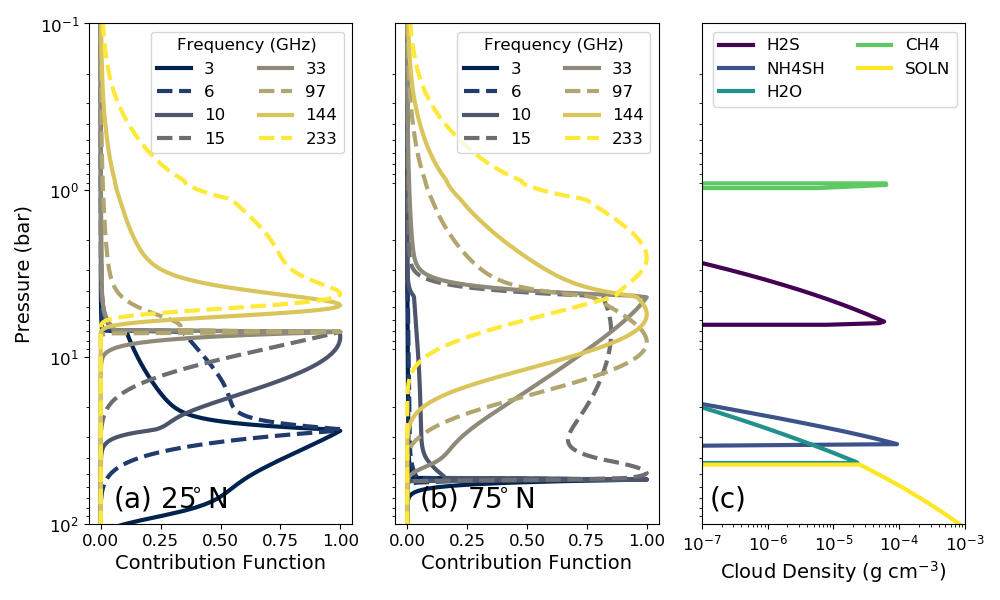
Figure 7: Normalized contribution function at each observed frequency for the best-fitting radiative transfer models at (a) 25^∘N and (b) 75^∘N. The spike in panel (b) at $\sim$40 bar is caused by the discontinuity in the vertical abundance profiles at the retrieved mixing pressure. (c) Cloud density as a function of pressure for clouds expected to form under thermochemical equilibrium assuming the abundance profiles in Figure 6.

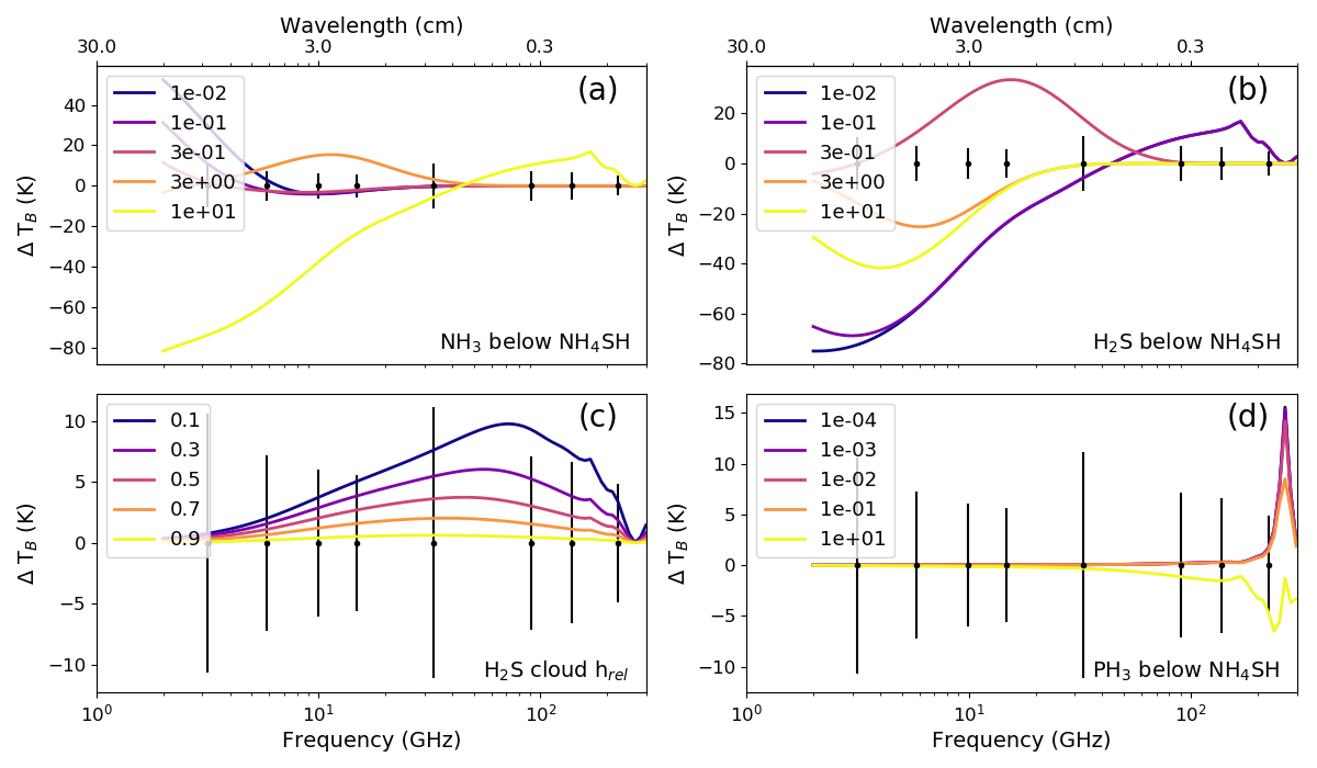
Figure 8: Effect of changing radiative transfer model parameters on the radio spectrum of Uranus. In each panel, one parameter was changed from its nominal value; the resulting model spectrum was subtracted from the nominal model such that $\Delta T_{B}$ represents the departure from the nominal model. Legend labels denote a multiplicative factor applied to the model parameter of interest, where 1.0 is the nominal value (30$\times$ Solar for H₂S and PH₃; 1$\times$ Solar for NH₃, 1.0 for H₂S h_rel). The black points plotted along the zero line show the size of the error bars on the data at the observed frequencies. All models were produced assuming viewing geometry from the sub-observer point.

Radiative transfer modeling was carried out within a Markov Chain Monte Carlo (MCMC) framework, implemented using the emcee Python package (Foreman-Mackey et al., 2013). Letting $\theta$ represent the set of free parameters in the model, the likelihood function $\ln p$ is given by

$$\ln p(T|\nu,\sigma,\theta)=-\frac{1}{2}\sum_{n}\Big{[}(T_{n}-T_{m}(\theta))^{2}\sigma_{n}^{-2}+\ln(2\pi\sigma_{n}^{-2})\Big{]}$$ (1)

where $\sigma_{n}^{2}$ is the variance of the measured brightness temperature $T_{n}$ at each frequency $\nu_{n}$. At each MCMC step, a set of test parameters $\theta$ is selected, a model brightness temperature $T_{m}(\theta)$ is generated by RadioBEAR at each frequency, and the likelihood function is evaluated. The result of many MCMC iterations is a joint probability distribution over the free parameters in the radiative transfer model. Each of the MCMC runs presented in this paper used 500 iterations and 40 walkers. As is standard practice with MCMC (Foreman-Mackey et al., 2013), we cut out the “burn-in” phase by using only the second half of the iterations to describe the posterior distribution; plotting the parameter values as a function of iteration confirmed that this procedure had worked as intended. We refer the interested reader to Hogg & Foreman-Mackey (2018) for an overview of how MCMC works and is used in astrophysics research.

3.3.1 Enriched Region

We first fit the radio-dark region at 25^∘N, chosen as the representative “enriched” or volatile-rich region because of its location at small emission angles with respect to the observer as well as relatively similar brightnesses at nearby latitudes, minimizing beam smearing effects. For computational efficiency, we simplified the full cloud-physics model to include only prescriptions for the NH₄SH cloud and the H₂S, NH₃, CH₄, and PH₃ ice clouds. The solution cloud beneath the NH₄SH cloud was ignored; this was a reasonable compromise because its location at $\sim$100 bar pressures is deeper than the observed frequencies probe (see Figure 7). The vertical abundance profile of H₂O as well as all other inputs (ortho-para fraction, adiabat) were set to their nominal values. We checked our simplified implementation against the full cloud-physics model, and found that the difference in brightness temperature between them was at least an order of magnitude smaller than the flux calibration errors at all frequencies. However, it should be noted that the MCMC retrieval estimates the NH₃ and H₂S abundances below the NH₄SH layer but above the solution cloud, i.e. at $\sim$50-100 bar. The solution cloud in the full model removes $\sim$5% of the deep H₂S and $\sim$25% of the deep NH₃; this is discussed further in Section 3.3.3. The retrieved values for all the parameters at 25^∘N are given in Table 3. The best-fitting model is compared to the data in Figure 9, and a “corner plot” displaying the one- and two-dimensional projections of the posterior probability distribution of the retrieved parameters is shown in Figure 10. The observed disk-averaged brightness temperatures are also reasonably well fit by the 25^∘ model (see Figure 3).

Parameter	2.5% ($-2\sigma$)	16% ($-1\sigma$)	Median	84% ($+1\sigma$)	97.5% ($+2\sigma$)	Abundance / Solar (1$\sigma$)
NH3 below NH4SH	$4.07\times 10^{-9}$	$2.63\times 10^{-7}$	$7.23\times 10^{-6}$	$8.49\times 10^{-5}$	$7.40\times 10^{-4}$	0.06${}^{+0.6}_{-0.04}$
H2S below NH4SH	$5.34\times 10^{-4}$	$6.88\times 10^{-4}$	$8.27\times 10^{-4}$	$1.12\times 10^{-3}$	$1.50\times 10^{-3}$	35.2${}^{+12.5}_{-5.9}$
H2S hrel	0.005	0.02	0.05	0.13	0.34	—
CH4 below NH4SH	$2.68\times 10^{-4}$	$1.77\times 10^{-3}$	$8.29\times 10^{-3}$	$2.39\times 10^{-2}$	$5.73\times 10^{-2}$	17${}^{+33}_{-14}$
ortho-para	0.03	0.19	0.58	0.87	0.97	—
PH3 below NH4SH	$4.52\times 10^{-9}$	$2.86\times 10^{-7}$	$3.43\times 10^{-6}$	$1.16\times 10^{-5}$	$2.72\times 10^{-5}$	18${}^{+43}_{-17}$
H2S above NH4SH	$4.29\times 10^{-4}$	$6.32\times 10^{-4}$	$8.09\times 10^{-4}$	$1.00\times 10^{-3}$	$1.31\times 10^{-3}$	34.4${}^{+8.3}_{-7.7}$
Deep H2S	$5.59\times 10^{-4}$	$7.20\times 10^{-4}$	$8.65\times 10^{-4}$	$1.17\times 10^{-3}$	$1.57\times 10^{-3}$	36.8${}^{+13.1}_{-6.2}$

Table 3: Values and errors for radiative transfer model parameters for the “enriched” region at 25^∘N. The median values are reported, along with the 16th/84th percentile values, which represent the 1$\sigma$ interval, and the 2.5/97.5 percentile values, which represent the 2$\sigma$ interval. The quantities below the horizontal line are not free parameters in the model, but can be determined from the retrieved vertical profiles. The values below the solution cloud are measured at 35 bar. The ortho-para fraction takes a value between 0 and 1, where 1 is “equilibrium” H₂ and 0 is “normal” H₂. The deep H₂S abundance refers to the model abundance below the water solution cloud.

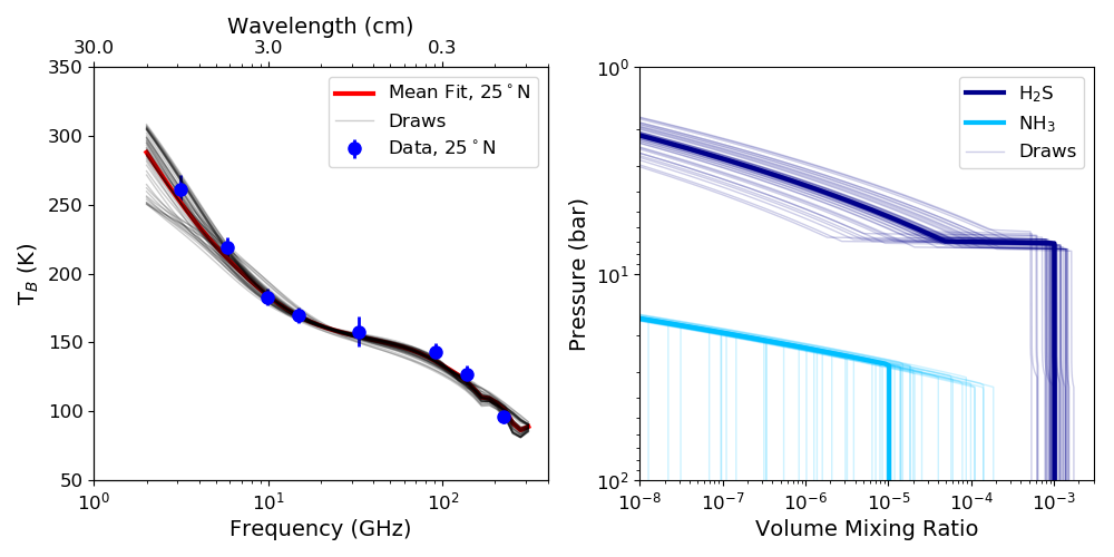
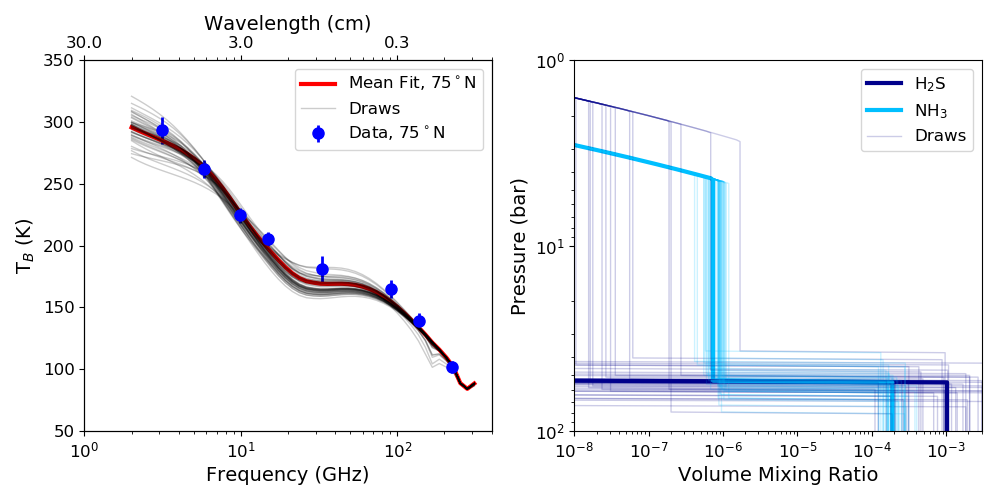
Figure 9: Left: Brightness temperature measurements of Uranus (blue dots) compared to our radiative transfer models at 25^∘N (top) and 75^∘N (bottom). The best-fitting model is shown as a thick red line, and 50 MCMC draws are shown as thin grey lines. Right: Abundance profiles of H₂S (dark blue) and NH₃ (light blue) for the best-fitting model (thick line) and the same 50 draws (thin lines) at 25^∘N (top) and 75^∘N (bottom). We refer the reader to Hogg & Foreman-Mackey (2018) for an explanation of the meaning of model draws.

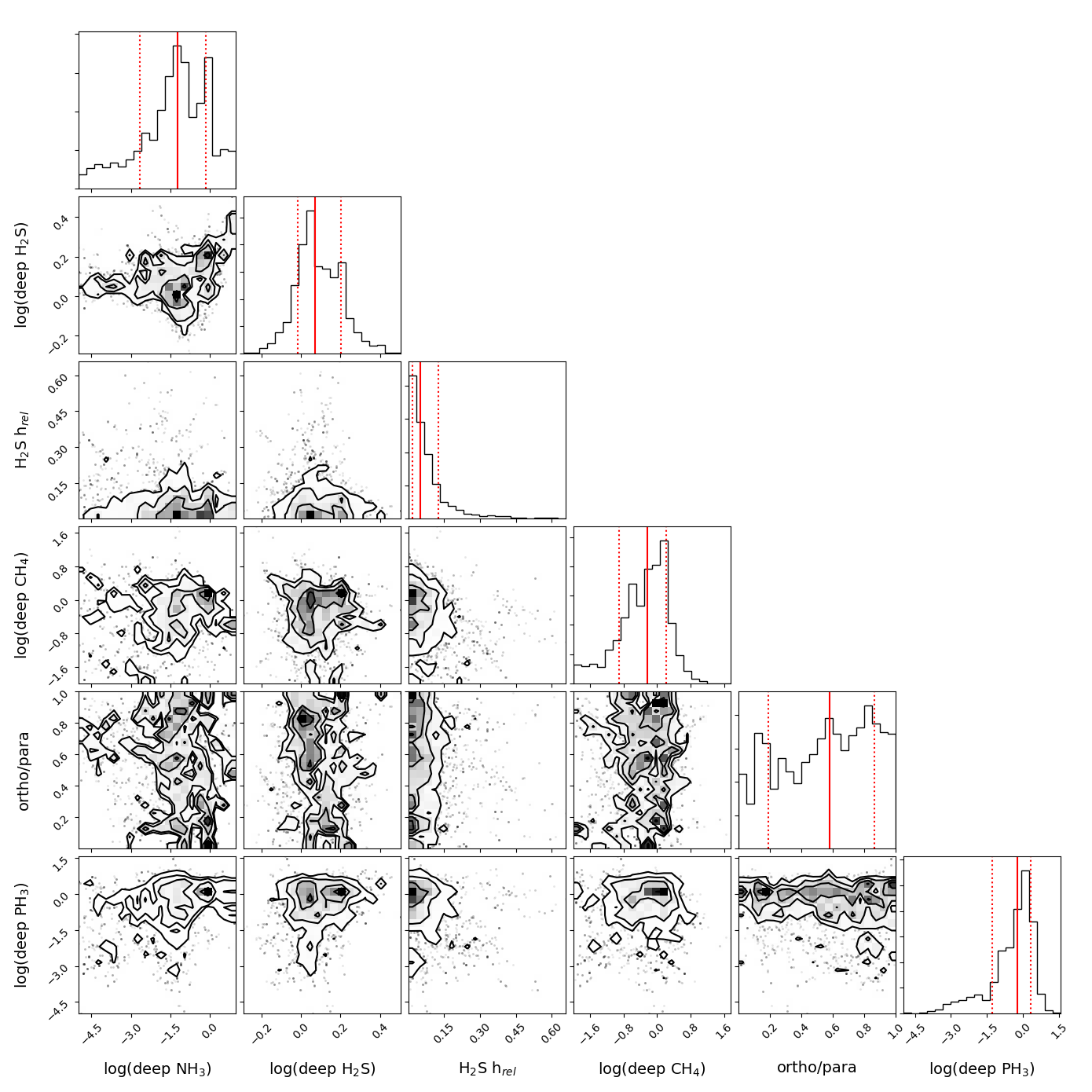
Figure 10: “Corner plot” showing the one-dimensional (top panels, corresponding to the label at the bottom of each column) and two-dimensional (other panels) projections of the posterior probability distribution of the MCMC-retrieved parameters for the radiative transfer models at 25^∘N. The mean value (solid red line) and 16th and 84th percentile (dotted red lines) of each probability distribution are plotted. We refer the reader to Hogg & Foreman-Mackey (2018) for an explanation of how to interpret a corner plot.

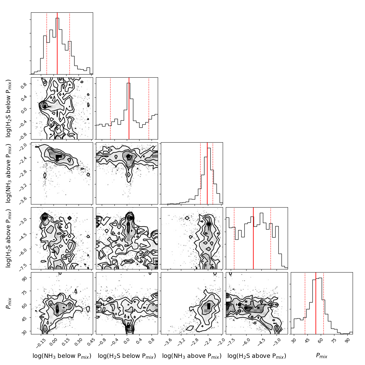
Figure 11: Same as Figure 10 but for the depleted model and data at 75^∘N.

The abundance of ammonia below the NH₄SH cloud is only weakly constrained in the enriched region, with a best-fitting value of 6% Solar but a 1$\sigma$ confidence interval from 0.2% to 70% Solar. This quantity is better constrained in the depleted north polar region, where the very low H₂S absorption allows our observations to probe deeper into the atmosphere (see Section 3.3.2). The hydrogen sulfide abundance takes a 1$\sigma$ value of $35.2_{-5.9}^{+12.3}\times$ Solar below the NH₄SH cloud, in excellent agreement with previous results (de Pater et al., 1991). The relative humidity of the H₂S ice cloud takes an 84th percentile value of 0.13, meaning that $h_{rel}<13$% is preferred to higher values. Models that include at least some PH₃ are preferred, as absorption from the pressure-broadened PH₃ line at 1.123 mm (266.9 GHz) is the only way in our model to decrease the brightness temperature at 1.3 mm relative to 2.1 mm. Indeed, a PH₃ abundance below $\sim$3% Solar is disfavored at the 2$\sigma$ level. However, the spectral slope within the 1.3 mm ALMA band is more consistent with models lacking phosphine absorption than models including it (see Figure 12). A detailed study of Uranus’s radio spectrum around the PH₃ $J=1\rightarrow 0$ absorption line at 1.123 mm (266.9 GHz) is required to confirm or rule out the presence of significant PH₃ in the Uranian troposphere. The methane abundance is only weakly constrained. Our retrieved abundance agrees with previous measurements at near-infrared and visible wavelengths, which range from $\sim$3 to $\sim$5% in the equatorial regions (Karkoschka & Tomasko, 2009; Tice et al., 2013; Sromovsky et al., 2014, 2019; Irwin et al., 2019), but is not as constraining as these studies. The average spin state of hydrogen (ortho-para) remains completely unconstrained by our data.

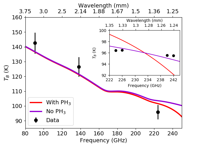
Figure 12: Main: ALMA data at 25^∘N (black points) plotted over radiative transfer models with 35$\times$ Solar phosphine (red line) and without any phosphine (purple line). The inclusion of phosphine marginally improves the fit. In this plot the error bars include the flux calibration error and are identical to those in the left panel of Figure 9. Inset: ALMA data in Band 6 (1.24-1.35 mm) split into its four spectral windows. We plot here only the error due to random noise, which is very small compared to the brightess of Uranus; the error bars are of the same order as the thickness of the data points. The radiative transfer models are normalized so that their value at 1.29 mm (233 GHz) is equal to the mean of the Band 6 data, to facilitate visual comparison of the spectral slopes. Here the inclusion of phosphine makes the spectral slope agreement poorer.

3.3.2 North Pole

We then modeled the brightness temperature of the depleted north polar region at 75^∘ N. Physically, the situation in the downwelling depleted region differs from that in the upwelling enriched region: the subsiding air is already depleted in condensible species, so strong subsaturations are likely at certain pressures. In addition, the depletion in abundances does not extend to infinite depth—the atmosphere must be well-mixed deeper than some pressure P_mix. Thus the deep abundance should remain the same as retrieved in the enriched region. With these considerations in mind, we employ a model for the depleted region that prescribes a step function in the H₂S and NH₃ abundances. We set the prior probability distribution functions of the deep abundances equal to the posterior probability distribution functions found for the enriched region; that is, the deep abundances are constrained to agree with the enriched region. The H₂S and NH₃ abundances are uniform above some mixing pressure $P_{mix}$ until the species reaches its condensation level; the depletion factor of each species and $P_{mix}$ are allowed to vary freely. The retrieved values for all the parameters at 75^∘N are given in Table 4. The best-fitting model is compared to the data in Figure 9, and a “corner plot” displaying the one- and two-dimensional projections of the posterior probability distribution of the retrieved parameters is shown in Figure 11.

Parameter	2.5% ($-2\sigma$)	16% ($-1\sigma$)	Median	84% ($+1\sigma$)	97.5% ($+2\sigma$)	Abundance / Solar (1$\sigma$)
NH3 below Pmix	$8.46\times 10^{-5}$	$1.00\times 10^{-4}$	$1.31\times 10^{-4}$	$1.86\times 10^{-4}$	$2.74\times 10^{-4}$	1.10${}^{+0.46}_{-0.26}$
H2S below Pmix	$8.46\times 10^{-5}$	$2.07\times 10^{-4}$	$8.46\times 10^{-4}$	$3.61\times 10^{-3}$	$6.41\times 10^{-3}$	36${}^{+118}_{-27}$
NH3 above Pmix	$1.09\times 10^{-7}$	$2.88\times 10^{-7}$	$4.67\times 10^{-7}$	$6.75\times 10^{-7}$	$9.53\times 10^{-7}$	$3.9^{+1.7}_{-1.5}\times 10^{-3}$
H2S above Pmix	—	—	—	$1.89\times 10^{-7}$	$1.11\times 10^{-6}$	$<$0.008
$P_{mix}$	30.64	42.23	54.59	63.23	75.58	—
Deep NH3	$1.02\times 10^{-4}$	$1.31\times 10^{-4}$	$1.71\times 10^{-4}$	$2.43\times 10^{-4}$	$3.92\times 10^{-4}$	1.44${}^{+0.60}_{-0.34}$

Table 4: Values and errors for radiative transfer model parameters for the “depleted” north polar region at 75^∘N. The median values are reported, along with the 16th/84th percentile values, which represent the 1$\sigma$ interval, and the 2.5/97.5 percentile values, which represent the 2$\sigma$ interval. The quantities below the horizontal line are not free parameters in the model, but can be determined from the retrieved vertical profiles. The deep NH₃ abundance refers to the model abundance below the H₂O solution cloud.

The MCMC simulation shows that strong depletions in both NH₃ and H₂S are required above the mixing pressure. The results are consistent with zero H₂S above the mixing pressure; the simulation yields a 1$\sigma$ upper limit of 0.8% Solar, which translates to at least $\sim$4000 times less H₂S above $P_{mix}$ than in the enriched region, i.e., an abundance $\lesssim$$2\times 10^{-7}$. The results do not constrain the H₂S abundance below $P_{mix}$ any more than did the enriched region model. Because so little H₂S absorption is present, the spectrum of the depleted north polar region is more sensitive than the enriched equatorial region to the NH₃ abundance below the mixing pressure, and this quantity is constrained to $1.10_{-0.26}^{+0.45}\times$ Solar (1$\sigma$). Above the mixing pressure, the model is consistent with a factor of $\sim$280 depletion in NH₃ in the north polar region compared to the enriched midlatitude region, i.e., an abundance of $\sim$$5\times 10^{-7}$. The retrieved mixing pressure of $55_{-12}^{+9}$ (1$\sigma$) is somewhat deeper than the level at which the NH₄SH cloud is expected to form in equilibrium ($\sim$35 bar); however, this value remains within the 95% (2$\sigma$) confidence interval. Thus it is a reasonable guess that the atmosphere transitions from well-mixed to depleted at the NH₄SH cloud.

3.3.3 RT Modeling Discussion

The good fit to the data provided by our cloud-physics model (Figure 9) lends strong support to a Uranian atmosphere dominated by H₂S absorption in the upwelling regions, with most or all NH₃ removed from the troposphere by the NH₄SH cloud. This model, which is similar to that of de Pater et al. (1989, 1991), permits significant H₂S above the NH₄SH cloud. The nitrogen-to-sulfur (N/S) ratio does not need to be tuned to very near unity as required by the H₂S-inclusive models of Hofstadter (1992). The midlatitudes are fit by a solar NH₃ abundance below the NH₄SH layer, which forms at a pressure of $\sim$35 bar. This is deeper than the midlatitude mixing pressure of $\sim$22 bar determined by Hofstadter et al. (1990); however, those authors did not consider the role of H₂S absorption on Uranus’s radio spectrum. In the downwelling north polar region, our model agrees well with the Hofstadter et al. (1990) and Hofstadter (1992) south polar region model: those authors required an NH₃ abundance of $\sim$$5\times 10^{-7}$ down to $\sim$50 bar pressures (they ignored H₂S gas opacity). All three of those requirements are within $1\sigma$ of our results, providing evidence that the north- and south-polar warm spots may arise from the same chemical processes.

The retrieved abundances derived in the previous subsections came from a simplified cloud-physics model that did not take into account the solution cloud at pressures deeper than 50 bars. Thus, to make inferences about the true deep abundances of nitrogen- and sulfur-bearing species, we returned to the full cloud-physics model of de Pater et al. (1991), which includes prescriptions for the deep water and water-solution clouds from Atreya & Romani (1985). We tuned the model such that the NH₃ and H₂S abundances between the solution cloud and the NH₄SH cloud matched our retrieved abundances of those species. For this purpose, we used the best-fitting H₂S abundance below the NH₄SH cloud from the enriched region and the best-fitting NH₃ abundance below $P_{mix}$ from the depleted region, since those were the best-constrained values and the two regions are assumed to be well-mixed below the mixing layer. This procedure yielded abundances in the deep troposphere of $1.7_{-0.4}^{+0.7}\times 10^{-4}$ (1.4${}_{-0.3}^{+0.6}$$\times$ Solar; 1$\sigma$) for NH₃ and $8.7_{-1.5}^{+3.1}\times 10^{-4}$ (37${}_{-6}^{+13}$$\times$ Solar; 1$\sigma$) for H₂S.

Using the NH₃/H₂S ratio as a proxy for the nitrogen/sulfur (N/S) ratio, our results provide a much stronger constraint on Uranus’s bulk atmospheric N/S ratio than previous work. We find N/S = $0.20_{-0.07}^{+0.08}$ (1$\sigma$), in agreement with de Pater et al. (1989, 1991), who required N/S$<0.2$. This is a very strong selective enrichment in sulfur considering the Solar N/S value of $\sim$5. Our observed sulfur-to-nitrogen ratio can be explained by an ice giant formation scenario in which volatiles were trapped as clathrate hydrates and then swept up by planetesimals (Hersant et al., 2004). Those authors argue that in the cold, ice-rich conditions of the outer disk, NH₃ and H₂S would be trapped very efficiently by clathration and accrete onto solid grains, while N₂ would remain in the gas phase. At the temperature and pressure of the outer disk, nearly all sulfur is in the form of H₂S, and the N₂:NH₃ ratio is roughly 10:1. Therefore, Uranus and Neptune should have accreted nearly all available sulfur but only a small fraction of available nitrogen, decreasing the N/S ratio by a factor of $\sim$20, which is close to what we observe.

4 Conclusions

The millimeter and radio observations presented here provide a unique view of Uranus’s troposphere: we provide the first published millimeter-wavelength maps of the planet, as well as the first VLA observations taken during northern summer. Our results are summarized as follows.

• High-spatial-resolution maps reveal a complex tropospheric circulation pattern, including thin, bright, likely downwelling bands at $\sim$0^∘N, 20^∘N, and 20^∘S in the 2 cm VLA and 2.1/3.1 mm ALMA maps. The identity of the absorber in these bands remains unknown, but variations in the relative humidity of H₂S or the methane abundance are good candidates to explain these features. Kinetic temperature variations may also play a role.

• The north polar region is approximately equal in brightness and extent to the south polar region observed three decades ago, with a radio brightness temperature $\sim$35 K brighter at 2 cm than the midlatitudes. The polar brightening can be observed over a large range of frequencies from 10 cm - 1 mm. Taken together with methane sensitive infrared measurements, this implies a single vertical cell of downwelling air from $\sim$0.1 to 50 bars. Radiative transfer modeling suggests the north polar region is depleted in ammonia to a similar degree as the south polar region observed 30 years ago; both have an NH₃ volume mixing ratio of $\sim$$5\times 10^{-7}$ above the $\sim$50 bar level and zero H₂S opacity.

• The radio spectrum of the dark upwelling midlatitude regions between $\sim$40^∘S and $\sim$40^∘N is consistent with a model in which all NH₃ is removed by the NH₄SH cloud at $\sim$35 bar, and constrains the deep H₂S abundance to $37_{-6}^{+13}\times$ Solar.

• The radio spectrum of the downwelling north polar region at latitudes north of $\sim$50^∘N is consistent with strong depletions in both ammonia and hydrogen sulfide from the top of the atmosphere down to a mixing pressure $P_{mix}=55_{-12}^{+9}$. The strong depletion in H₂S in this region permits the deep NH₃ abundance to be well constrained, taking a value of $1.4_{-0.3}^{+0.6}\times$ Solar.

• The deep sulfur-to-nitrogen ratio in Uranus’s troposphere is N/S = $0.20_{-0.07}^{+0.08}$ (note protosolar N/S $\sim$ 5), assuming the Atreya & Romani (1985) prescription for the water-solution cloud at pressures deeper than 50 bars and no temperature difference between equator and pole. This is the most stringent constraint on that ratio to date.

• The phosphine abundance in the ice giants remains unknown; the observations presented in this work are only sensitive to pressure-broadened phosphine spectral lines at the 2$\sigma$ level in one band (ALMA Band 6; 1.3 mm), and the spectral slope in this band does not support a pressure-broadened phosphine line.

This paper lays the groundwork for more detailed studies of Uranus’s tropospheric circulation and composition with the upcoming Next-Generation Very Large Array (NGVLA). The NGVLA will perform 10 cm and 20 cm observations at resolutions of $\sim$3 mas and $\sim$10 mas, respectively, permitting a much stronger constraint on the ammonia abundance in the ice giants. Observations from 3 cm to 3 mm at resolutions down to 0.1 mas will resolve the new dark and bright bands discovered in this work well enough to extract robust brightness temperature measurements from those regions; applying radiative transfer models may identify the absorbers responsible for these bands. An outline of the solar system science that will become possible with the ngVLA is given in de Pater et al. (2018).

adiobear, scipy, emcee, CASA, MIRIAD

Appendix A Meridional Temperature Gradients

The radio occultation experiment aboard the Voyager 2 spacecraft determined the temperature-pressure profile in Uranus down to roughly 2.7 bar (Lindal et al., 1987); however, this measurement was made using two occultations between 0^∘ and -10^∘ latitude, so meridional differences were not observed. The IRIS instrument determined the temperature structure down to $\sim$0.6 bar as a function of latitude, finding temperature differences smaller than 2 K (Pearl et al., 1990). Similarly small temperature differences have also been observed in the upper troposphere from more recent ground-based studies (Roman et al., 2020). The latitudinal temperature structure of Uranus has not been directly observed below 1 bar. Most atmospheric models predict that meridional temperature gradients should be small because the orbital period is much shorter than the radiative relaxation time in Uranus’s troposphere (Wallace, 1983; Friedson & Ingersoll, 1987; Conrath et al., 1990); however, recent calculations have cast doubt on the radiative timescales used in those papers (Li et al., 2018). We must therefore consider the possibility that the observed brightness temperature difference between the midlatitude and polar regions is driven primarily by differences in kinetic temperature, instead of differences in composition as assumed in the main text. The strength of an absorption feature is set by both the abundance profile of the absorbing species and the atmospheric temperature profile. To disentangle temperature and abundance is an underconstrained problem; however, a large midlatitude-to-pole temperature difference between $\sim$0.6 and 50 bar is generally considered unlikely based on several lines of evidence. These have been summarized convincingly by Hofstadter & Butler (2003), and here we leverage our new data to expand upon the arguments of those authors.

The radio/millimeter spectra at the midlatitudes and poles cannot both be fit with the same composition unless a highly unphysical temperature-pressure profile is assumed. The latent heat of condensation of H₂S (or H₂S/NH₃ in the NH₄SH cloud) at saturation is very small compared to the enthalpy of a parcel of air in Uranus, so the difference between a moist and dry adiabat is very small. However, if the requirement to fit the Voyager data at pressures less than 0.6 bar is relaxed, warmer or cooler adiabats can be considered. Starting with our best-fitting gas abundances and vertical temperature structure in the midlatitude region (Section 3.3.1), we tried using warmer adiabatic profiles; a sample result is shown in Figure A1. No adiabatic profile can effectively fit the north polar data. To achieve a reasonable fit to the observed north polar spectrum using only kinetic temperature changes requires many unphysical kinks in the temperature structure (Figure A1). The “solutions” we find require a strongly superadiabatic lapse rate near the H₂S ice cloud level to bring H₂S condensation high in the atmosphere, and a strongly subadiabatic lapse rate deper than that to keep the NH₄SH cloud deep enough. Overall, we find that the spectra, and in particular the millimeter wavelengths, are highly sensitive to the pressure level of the H₂S and NH₄SH clouds; the kinetic temperature must be tuned very finely to place these at the correct equilibrium level. It is worth noting that a discontinuity in the temperature profile at a condensation layer is possible if a large vertical gradient in atmospheric molecular weight is also present, as has been suggested for both the methane and H₂O cloud layers (Guillot, 1995; Cavalié et al., 2017, 2020). However, the abundances of NH₃ and H₂S have a factor of $\gtrsim$25 less effect on the atmospheric molecular weight than those of CH₄ and H₂O, so this effect is not expected to be important near the NH₄SH or H₂S cloud layers.

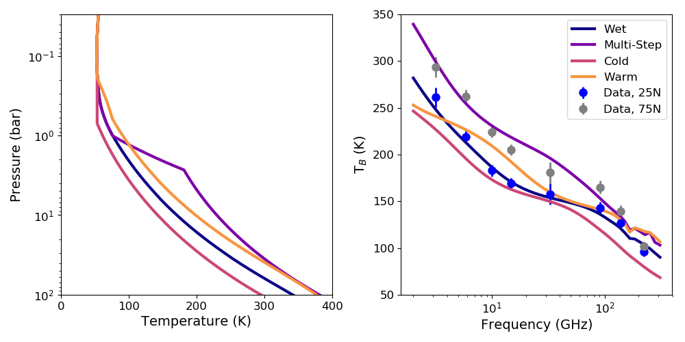
Figure A1: Effect of temperature profile perturbations on the radio/millimeter spectrum of Uranus. Using the same chemical abundances as for our best-fitting model at 25^∘N, we consider a wet adiabat (blue line) and a warmer and cooler adiabat (orange and salmon lines). We also attempt to perturb the temperature profile ad-hoc until a reasonable fit to the north-polar-region data is achieved (purple line).

Hofstadter & Butler (2003) considered the complementary situation, in which the bright polar region followed an adiabat and the equatorial region was fit using strongly subadiabatic temperature profiles. This goes contrary to most theory, which generally predicts that the pole should be more stably stratified (Briggs & Andrew, 1980; Wallace, 1983; Friedson & Ingersoll, 1987), but shall be considered regardless. In this case, the temperature profiles at the midlatitudes and poles were both forced to fit the Voyager data, but allowed to diverge below. Hofstadter & Butler (2003) note that the temperature differences needed to make this work, which reach 90 K at 20 bar pressure, imply a vertical wind shear of $-100$ m s^-1 per scale height at 20 bar by the thermal wind equation. However, they stop short of integrating the thermal wind equation vertically to produce a geostrophic wind profile. We have done this, and find that the winds must be supersonic deeper than $\sim$20 bar, which is unphysical. It is worth noting that the thermal wind equation assumes a compositionally constant atmosphere wherein density differences are due to temperature only. Significant meridional gradients in composition could arise on Uranus via gradients in the methane abundance, since methane accounts for up to 5% of the troposphere by volume and is much heavier than hydrogen and helium (Sun et al., 1991; Tollefson et al., 2018). However, methane is observed to be depleted in the poles relative to the midlatitudes (Karkoschka & Tomasko, 2009; Tice et al., 2013; Sromovsky et al., 2014, 2019; Irwin et al., 2019), so the implied compositional (and therefore density) gradients would lead to even larger vertical wind shear. The observed thermal wind (e.g., Sromovsky et al., 2015) also points, again by the thermal wind equation, to a warmer midlatitude region than polar region.

Taken together, these arguments show that composition is the primary driver of the observed brightness temperature differences at millimeter and radio wavelengths. However, the possibility that both temperature and composition change between the midlatitudes and poles cannot be ruled out. A different assumed polar temperature profile would have a relatively small but perhaps non-negligible effect on the deep NH₃ abundance retrieved in this paper.

References

- Allison et al. (1991) Allison, M., Beebe, R. F., Conrath, B. J., Hinson, D. P., & Ingersoll, A. P. 1991, Uranus atmospheric dynamics and circulation., ed. J. T. Bergstralh, E. D. Miner, & M. S. Matthews, 253–295
- Asplund et al. (2009) Asplund, M., Grevesse, N., Sauval, A. J., & Scott, P. 2009, ARA&A, 47, 481, doi: 10.1146/annurev.astro.46.060407.145222
- Atreya & Romani (1985) Atreya, S. K., & Romani, P. N. 1985, Photochemistry and clouds of Jupiter, Saturn and Uranus., ed. G. E. Hunt, 17–68
- Borysow & Frommhold (1986) Borysow, A., & Frommhold, L. 1986, ApJ, 304, 849, doi: 10.1086/164221
- Briggs & Andrew (1980) Briggs, F. H., & Andrew, B. H. 1980, Icarus, 41, 269, doi: 10.1016/0019-1035(80)90010-X
- Brogan et al. (2018) Brogan, C. L., Hunter, T. R., & Fomalont, E. B. 2018, arXiv e-prints. https://arxiv.org/abs/1805.05266
- Butler et al. (2001) Butler, B. J., Steffes, P. G., Suleiman, S. H., Kolodner, M. A., & Jenkins, J. M. 2001, Icarus, 154, 226, doi: 10.1006/icar.2001.6710
- Cavalié et al. (2017) Cavalié, T., Venot, O., Selsis, F., et al. 2017, Icarus, 291, 1, doi: 10.1016/j.icarus.2017.03.015
- Cavalié et al. (2020) Cavalié, T., Venot, O., Miguel, Y., et al. 2020, Space Sci. Rev., 216, 58, doi: 10.1007/s11214-020-00677-8
- Conrath et al. (1990) Conrath, B. J., Gierasch, P. J., & Leroy, S. S. 1990, Icarus, 83, 255, doi: 10.1016/0019-1035(90)90068-K
- de Kleer et al. (2015) de Kleer, K., Luszcz-Cook, S., de Pater, I., Ádámkovics, M., & Hammel, H. B. 2015, Icarus, 256, 120, doi: 10.1016/j.icarus.2015.04.021
- de Pater (2018) de Pater, I. 2018, Nature Astronomy, 2, 364, doi: 10.1038/s41550-018-0457-5
- de Pater et al. (2005) de Pater, I., DeBoer, D., Marley, M., Freedman, R., & Young, R. 2005, Icarus, 173, 425, doi: 10.1016/j.icarus.2004.06.019
- de Pater & Gulkis (1988) de Pater, I., & Gulkis, S. 1988, Icarus, 75, 306, doi: 10.1016/0019-1035(88)90007-3
- de Pater et al. (1989) de Pater, I., Romani, P. N., & Atreya, S. K. 1989, Icarus, 82, 288, doi: 10.1016/0019-1035(89)90040-7
- de Pater et al. (1991) —. 1991, Icarus, 91, 220, doi: 10.1016/0019-1035(91)90020-T
- de Pater et al. (2016) de Pater, I., Sault, R. J., Butler, B., DeBoer, D., & Wong, M. H. 2016, Science, 352, 1198, doi: 10.1126/science.aaf2210
- de Pater et al. (2019) de Pater, I., Sault, R. J., Wong, M. H., et al. 2019, Icarus, 322, 168, doi: 10.1016/j.icarus.2018.11.024
- de Pater et al. (2015) de Pater, I., Sromovsky, L. A., Fry, P. M., et al. 2015, Icarus, 252, 121, doi: 10.1016/j.icarus.2014.12.037
- de Pater et al. (2011) de Pater, I., Sromovsky, L. A., Hammel, H. B., et al. 2011, Icarus, 215, 332, doi: 10.1016/j.icarus.2011.06.022
- de Pater et al. (2014) de Pater, I., Fletcher, L. N., Luszcz-Cook, S., et al. 2014, Icarus, 237, 211, doi: 10.1016/j.icarus.2014.02.030
- de Pater et al. (2018) de Pater, I., Butler, B., Sault, R. J., et al. 2018, Astronomical Society of the Pacific Conference Series, Vol. 517, Potential for Solar System Science with the ngVLA, ed. E. Murphy, 49
- Fegley & Prinn (1986) Fegley, B., J., & Prinn, R. G. 1986, ApJ, 307, 852, doi: 10.1086/164472
- Flasar et al. (1987) Flasar, F. M., Conrath, B. J., Gierasch, P. J., & Pirraglia, J. A. 1987, J. Geophys. Res., 92, 15011, doi: 10.1029/JA092iA13p15011
- Fletcher et al. (2020) Fletcher, L. N., de Pater, I., Orton, G. S., et al. 2020, Space Sci. Rev., 216, 21, doi: 10.1007/s11214-020-00646-1
- Foreman-Mackey et al. (2013) Foreman-Mackey, D., Hogg, D. W., Lang, D., & Goodman, J. 2013, PASP, 125, 306, doi: 10.1086/670067
- Friedson & Ingersoll (1987) Friedson, J., & Ingersoll, A. P. 1987, Icarus, 69, 135, doi: 10.1016/0019-1035(87)90010-8
- Griffin & Orton (1993) Griffin, M. J., & Orton, G. S. 1993, Icarus, 105, 537, doi: 10.1006/icar.1993.1147
- Guillot (1995) Guillot, T. 1995, Science, 269, 1697, doi: 10.1126/science.7569896
- Gulkis & de Pater (1984) Gulkis, S., & de Pater, I. 1984, in NASA Conference Publication, Vol. 2330, NASA Conference Publication, ed. J. T. Bergstralh
- Gulkis et al. (1978) Gulkis, S., Janssen, M. A., & Olsen, E. T. 1978, Icarus, 34, 10, doi: 10.1016/0019-1035(78)90120-3
- Hersant et al. (2004) Hersant, F., Gautier, D., & Lunine, J. I. 2004, Planet. Space Sci., 52, 623, doi: 10.1016/j.pss.2003.12.011
- Hoffman et al. (2001) Hoffman, J. P., Steffes, P. G., & DeBoer, D. R. 2001, Icarus, 152, 172, doi: 10.1006/icar.2001.6622
- Hofstadter (1992) Hofstadter, M. D. 1992, PhD thesis, California Institute of Technology, Pasadena.
- Hofstadter et al. (1990) Hofstadter, M. D., Berge, G. L., & Muhleman, D. O. 1990, Icarus, 84, 261, doi: 10.1016/0019-1035(90)90170-E