Abstract

We propose a new reinforcement learning algorithm derived from a regularized linear-programming formulation of optimal control in MDPs. The method is closely related to the classic Relative Entropy Policy Search (REPS) algorithm of Peters et al., (2010), with the key difference that our method introduces a Q-function that enables efficient exact model-free implementation. The main feature of our algorithm (called Q-REPS) is a convex loss function for policy evaluation that serves as a theoretically sound alternative to the widely used squared Bellman error. We provide a practical saddle-point optimization method for minimizing this loss function and provide an error-propagation analysis that relates the quality of the individual updates to the performance of the output policy. Finally, we demonstrate the effectiveness of our method on a range of benchmark problems.

1 INTRODUCTION

While the squared Bellman error is a broadly used loss function for approximate dynamic programming and reinforcement learning (RL), it has a number of undesirable properties: it is not directly motivated by standard Markov Decission Processes (MDP) theory, not convex in the action-value function parameters, and RL algorithms based on its recursive optimization are known to be unstable (Geist et al.,, 2017; Mehta and Meyn,, 2020). In this paper, we offer a remedy to these issues by proposing a new RL algorithm utilizing an objective-function free from these problems. Our approach is based on the seminal Relative Entropy Policy Search (REPS) algorithm of Peters et al., (2010), with a number of newly introduced elements that make the algorithm significantly more practical.

While REPS is elegantly derived from a principled linear-programing (LP) formulation of optimal control in MDPs, it has the serious shortcoming that its faithful implementation requires access to the true MDP for both the policy evaluation and improvement steps, even at deployment time. The usual way to address this limitation is to use an empirical approximation to the policy evaluation step and to project the policy from the improvement step into a parametric space (Deisenroth et al.,, 2013), losing all the theoretical guarantees of REPS in the process.

In this work, we propose a new algorithm called Q-REPS that eliminates this limitation of REPS by introducing a simple softmax policy improvement step expressed in terms of an action-value function that naturally arises from a regularized LP formulation. The action-value functions are obtained by minimizing a convex loss function that we call the logistic Bellman error (LBE) due to its analogy with the classic notion of Bellman error and the logistic loss for logistic regression. The LBE has numerous advantages over the most commonly used notions of Bellman error: unlike the squared Bellman error, the logistic Bellman error is convex in the action-value function parameters, smooth, and has bounded gradients (see Figure 1). This latter property obviates the need for the heuristic technique of gradient clipping (or using the Huber loss in place of the square loss), a commonly used optimization trick to improve stability of training of deep RL algorithms (Mnih et al.,, 2015).

Besides the above favorable properties, Q-REPS comes with rigorous theoretical guarantees that establish its convergence to the optimal policy under appropriate conditions. Our main theoretical contribution is an error-propagation analysis that relates the quality of the optimization subroutine to the quality of the policy output by the algorithm, showing that convergence to the optimal policy can be guaranteed if the optimization errors are kept sufficiently small. Together with another result that establishes a bound on the bias of the empirical LBE in terms of the regularization parameters used in Q-REPS, this justifies the approach of minimizing the empirical objective under general conditions. For the concrete setting of factored linear MDPs, we provide a bound on the rate of convergence.

Our main algorithmic contribution is a saddle-point optimization framework for optimizing the empirical version of the LBE that formulates the minimization problem as a two-player game between a learner and a sampler. The learner plays stochastic gradient descent (SGD) on the samples proposed by the sampler, and the sampler updates its distribution over the sample transitions in response to the observed Bellman errors. We evaluate the resulting algorithm experimentally on a range of standard benchmarks, showing excellent empirical performance of Q-REPS.

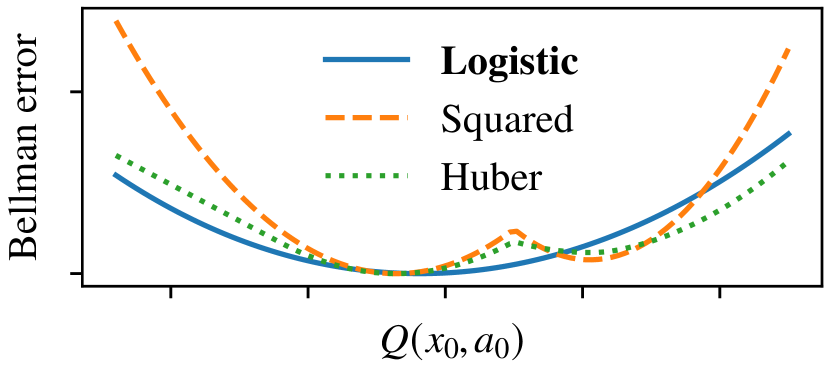
Figure 1: Squared Bellman error considered harmful: Loss functions plotted as a function of the Q-value at a fixed state-action pair while keeping other values fixed.

Related Work.

Despite the enormous empirical successes of deep reinforcement learning, we understand little about the convergence of the algorithms that are commonly used. The use of the squared Bellman error for deep reinforcement learning has been popularized in the breakthrough paper of Mnih et al., (2015), and has been exclusively used for policy evaluation ever since. Indeed, while several algorithmic improvements have been proposed for improving policy updates over the past few years, the squared Bellman error remained a staple: among others, it is used for policy evaluation in TRPO (Schulman et al.,, 2015), SAC (Haarnoja et al.,, 2018), A3C (Mnih et al.,, 2016), TD3 (Fujimoto et al.,, 2018), MPO (Abdolmaleki et al.,, 2018) and POLITEX (Abbasi-Yadkori et al.,, 2019). Despite its extremely broad use, the squared Bellman error suffers from a range of well-known issues pointed out by several authors including Sutton and Barto, (2018, Chapter 11.5), Geist et al., (2017), and Mehta and Meyn, (2020). While some of these have been recently addressed by Dai et al., (2018) and Feng et al., (2019), several concerns remain.

On the other hand, the RL community has been very productive in developing novel policy-improvement rules: since the seminal work of Kakade and Langford, (2002) established the importance of soft policy updates for dealing with policy-evaluation errors, several practical update rules have been proposed and applied successfully in the context of deep RL—see the list we provided in the previous paragraph. Many of these soft policy updates are based on the idea of entropy regularization, first explored by Kakade, (2001) and Ziebart et al., (2008) and inspiring an impressive number of followup works eventually unified by Neu et al., (2017) and Geist et al., (2019). A particularly attractive feature of entropy-regularized methods is that they often come with a closed-form “softmax” policy update rule that is easily expressed in terms of an action-value function. A limitation of these methods is that they typically don’t come with a theoretically well-motivated loss function for estimating the value functions and end up relying on the squared Bellman error. One notable exception is the REPS algorithm of Peters et al., (2010) that comes with a natural loss function for policy evaluation, but no tractable policy-update rule.

The main contribution of our work is proposing Q-REPS, a mirror-descent algorithm that comes with both a natural loss function and an explicit and tractable policy update rule, both derived from an entropy-regularization perspective. These properties make it possible to implement Q-REPS entirely faithfully to its theoretical specification in a deep reinforcement learning context, modulo the step of using a neural network for parametrizing the Q function. This implementation is justified by our main theoretical result, an error propagation analysis accounting for the optimization and representation errors.

Our error propagation analysis is close in spirit to that of Scherrer et al., (2015), recently extended to entropy-regularized approximate dynamic programming algorithms by Geist et al., (2019), Vieillard et al., 2020a , and Vieillard et al., 2020b . One major difference between our approaches is that their guarantees depend on the $\ell_{p}$ norms of the policy evaluation errors, but still optimize squared-Bellman-error-like quantities that only serve as proxy for these errors. In contrast, our analysis studies the propagation of the optimization errors on the objective function that is actually optimized by the algorithm.

Notation.

We use $\left\langle\cdot,\cdot\right\rangle$ to denote inner products in Euclidean space and ₊ to denote the set of non-negative real numbers. For two vectors $v,w\in{}^{m}$, we will use the notation $v\geq w$ to denote elementwise inequality holding in the sense $v-w\in{}_{+}^{m}$. We will often write indefinite sums $\sum_{x,a}$ to denote sums over the entire state-action space $\mathcal{X}\times\mathcal{A}$, and write $p(x,a)\propto q(x,a)$ to signify that $p(x,a)=q(x,a)/\sum_{x^{\prime},a^{\prime}}q(x^{\prime},a^{\prime})$ for a nonnegative function $q$ over $\mathcal{X}\times\mathcal{A}$.

2 BACKGROUND

Consider a Markov decision process (MDP, Puterman,, 1994) defined by the tuple $M=(\mathcal{X},\mathcal{A},P,r)$, where $\mathcal{X}$ is the state space, $\mathcal{A}$ is the action space, $P$ is the transition function with $P(\cdot|x,a)$ denoting the distribution of the follow-up state $x^{\prime}$ after taking action $a\in\mathcal{A}$ in state $x\in\mathcal{X}$, and $r$ is the reward function mapping state-action pairs to rewards with $r(x,a)$ denoting the reward of being in state $x$ and taking action $a$. For simplicity of presentation, we assume that the rewards are deterministic and bounded in $[0,1]$, and that the state action spaces are finite (but potentially very large). An MDP models a sequential interaction process between an agent and its environment where in each round $t$, the agent observes state $x_{t}\in\mathcal{X}$, selects action $a_{t}\in\mathcal{A}$, moves to the next state $x_{t+1}\sim P(\cdot|x_{t},a_{t})$, and obtains reward $r(x_{t},a_{t})$. The goal of the agent is to select actions so as to maximize the normalized discounted return $R=(1-\gamma)\mathbb{E}\left[\sum_{t=0}^{\infty}\gamma^{t}r(x_{t},a_{t})\right]$, where $\gamma\in(0,1)$ is the discount factor and the state $x_{0}$ is drawn from a fixed initial-state distribution $\nu_{0}$.

We will heavily rely on a linear programming (LP) characterization of optimal policies originally due to Manne,, 1960. This approach aims to directly find a normalized discounted state-action occupancy measure (in short, occupancy measure) $\mu(x,a)=(1-\gamma)\mathbb{E}\left[\sum_{t=0}^{\infty}\gamma^{t}\mathbb{I}_{\left\{(x_{t},a_{t})=(x,a)\right\}}\right]$ with $x_{0}\sim\nu_{0}$ that maximizes the discounted return that can simply be written as $R=\sum_{x,a}\mu(x,a)r(x,a)$. From every valid occupancy measure $\mu$, one can derive a stationary stochastic policy (in short, policy) $\pi_{\mu}$ defined as the conditional distribution $\pi_{\mu}(a|x)=\mu(x,a)/\sum_{a^{\prime}}\mu(x,a^{\prime})$ over actions $a$ for each state $x$. Following the policy $\pi_{\mu}$ by drawing each action $a_{t}\sim\pi(\cdot|x_{t})$ can be shown to yield $\mu$ as the occupancy measure. We briefly describe the characterization of optimal policies in these terms below, and refer the interested reader to Section 6.9 of Puterman, (1994) for a more detailed discussion.

For a compact notation, we will represent the decision variables $\mu$ as vectors in ^X×A and introduce the linear operator $P^{\mathsf{\scriptscriptstyle T}}:{}^{\mathcal{X}\times\mathcal{A}}\rightarrow{}^{\mathcal{X}}$ defined for each $\mu$ through $(P^{\mathsf{\scriptscriptstyle T}}\mu)(x^{\prime})=\sum_{x,a}P(x^{\prime}|x,a)\mu(x,a)$ for all $x^{\prime}$. Similarly, we define the operator $E^{\mathsf{\scriptscriptstyle T}}$ acting on $\mu$ through the assignment $(E^{\mathsf{\scriptscriptstyle T}}\mu)(x)=\sum_{a}\mu(x,a)$ for all $x$. With this notation, the task of finding an optimal occupancy measure can be written as the solution of the following linear program:

$$\begin{split}\text{maximize}_{\mu\in{}^{\mathcal{X}\times\mathcal{A}}_{+}}\quad&\left\langle\mu,r\right\rangle\\ \text{s.t.}\quad&E^{\mathsf{\scriptscriptstyle T}}\mu=\gamma P^{\mathsf{\scriptscriptstyle T}}\mu+(1-\gamma)\nu_{0}.\end{split}$$ (1)

The above set of constraints is known to uniquely characterize the set of all valid occupancy measures, which set will be denoted as $\mathcal{M}^{*}$ from here on. Due to this property, any solution $\mu^{*}$ of the LP maximizes the total discounted return and the corresponding policy $\pi^{*}=\pi_{\mu^{*}}$ is optimal in the sense that choosing actions as $a_{t}\sim\pi^{*}(\cdot|x_{t})$ yields maximal return. The dual of the linear program (1) is

$$\begin{split}\text{minimize}_{V\in{}^{\mathcal{X}}}\quad&(1-\gamma)\left\langle\nu_{0},V\right\rangle\\ \text{s.t.}\quad&EV\geq r+\gamma PV,\end{split}$$ (2)

where we used the adjoint operators $E$ and $P$, acting on $V$ as $(EV)(x,a)=V(x)$ and $(PV)(x,a)=\sum_{x^{\prime}}P(x^{\prime}|x,a)V(x^{\prime})$ for all $x,a$. The solution of this LP can be shown to be equivalent to the celebrated Bellman optimality equations in the sense that the so-called optimal value function $V^{*}$ is an optimal solution of this LP, and is the unique optimal solution if $\nu_{0}$ has full support over the state space.

Relative Entropy Policy Search.

Our approach is directly inspired by the seminal relative entropy policy search (REPS) algorithm proposed by Peters et al., (2010). The core ideas underlying REPS are adding a strongly convex regularization function to the objective of the LP (1) and relaxing the primal constraints through the use of a feature map $\psi:\mathcal{X}\rightarrow{}^{m}$. Introducing the operator $\Psi^{\mathsf{\scriptscriptstyle T}}$ acting on $q\in{}^{\mathcal{X}}$ as $\Psi^{\mathsf{\scriptscriptstyle T}}q=\sum_{x}q(x)\psi(x)$, and letting $\mu_{0}$ be an arbitrary state-action distribution, REPS is defined as an iterative optimization scheme that produces a sequence of occupancy measures as follows:

$$\begin{split}\mu_{k+1}=\max_{\mu\in{}^{\mathcal{X}\times\mathcal{A}}_{+}}\quad&\left\langle\mu,r\right\rangle-\frac{1}{\eta}D\left(\mu\middle\|\mu_{k}\right)\\ \text{s.t.}\quad&\Psi^{\mathsf{\scriptscriptstyle T}}E^{\mathsf{\scriptscriptstyle T}}\mu=\Psi^{\mathsf{\scriptscriptstyle T}}\left(\gamma P^{\mathsf{\scriptscriptstyle T}}\mu+(1-\gamma)\nu_{0}\right).\end{split}$$ (3)

Here, $D\left(\mu\middle\|\mu^{\prime}\right)$ is the unnormalized relative entropy (or Kullback–Leibler divergence) between the distributions $\mu$ and $\mu^{\prime}$ defined as $D\left(\mu\middle\|\mu^{\prime}\right)=\sum_{x,a}\bigl{(}\mu(x,a)\bigl{(}\log\frac{\mu(x,a)}{\mu^{\prime}(x,a)}-1\bigr{)}+\mu^{\prime}(x,a)\bigr{)}$. Introducing the notation $V_{\theta}=\Psi\theta$ and $\delta_{\theta}=r+\gamma PV_{\theta}-EV_{\theta}$, the unique optimal solution to this optimization problem can be written as

$$\mu_{k+1}(x,a)=\mu_{k}(x,a)e^{\eta\left(\delta_{\theta_{k}}(x,a)-\rho_{k}\right)},$$ (4)

where $\rho_{k}$ is a normalization constant and $\theta_{k}$ is given as the minimizer of the dual function given as

$$\mathcal{G}_{k}(\theta)=\sum_{x,a}\mu_{k}(x,a)e^{\eta\delta_{\theta}(x,a)}+(1-\gamma)\left\langle\nu_{0},V_{\theta}\right\rangle.$$ (5)

As highlighted by Zimin and Neu, (2013) and Neu et al., (2017), REPS can be seen as a mirror descent algorithm (Martinet,, 1970; Rockafellar,, 1976; Beck and Teboulle,, 2003), and thus its iterates $\mu_{k}$ are guaranteed to converge to an optimal occupancy measure $\mu^{*}$.

Despite its exceptional elegance, the formulation above has a number of features that limit its practical applicability. One very serious limitation of REPS is that its output policy $\pi_{K}$ involves an expectation with respect to the transition function, thus requiring knowledge of $P$ to run the policy. Another issue is that optimizing an empirical version of the loss (5) as originally proposed by Peters et al., (2010) may be problematic due to the empirical loss being a biased estimator of the true objective (5) caused by the conditional expectation appearing in the exponent.

Deep $Q$-learning.

Let us contrast REPS with the emblematic deep RL approach of Deep Q Networks (DQN) as proposed by Mnih et al., (2015). This algorithm aims to approximate the optimal action-value function $Q^{*}(x,a)$ which is known to characterize optimal behaviors: any policy that puts all probability mass on $\mathop{\mbox{ arg\,max}}_{a}Q^{*}(x,a)$ is optimal. Using the notation $\left\|f\right\|_{\mu}^{2}=\sum_{x,a}\mu(x,a)f^{2}(x,a)$, the main idea of DQN is to sequentially compute approximations of $Q^{*}$ by minimizing the squared Bellman error:

$$Q_{k+1}=\mathop{\mbox{ arg\,min}}_{Q\in\mathcal{Q}}\left\|r+\gamma PV_{Q}-Q\right\|^{2}_{\mu_{k}},$$ (6)

where $\mathcal{Q}$ is some class of action-value functions (e.g., a class of neural networks), $V_{Q}(x)=\max_{a}Q(x,a)$, and $\mu_{k}$ is the state distribution generated by the policy $\pi_{k}$. A major advantage of this formulation is that, having access to Q-functions, it is trivial to compute policy updates, typically by choosing near-greedy policies with respect to $Q_{k}$. However, it is well known that the squared Bellman error objective above suffers from a number of serious problems: its lack of convexity in $Q$ prevents efficient optimization even under the simplest parametrizations, and the conditional expectation appearing within the squared norm makes its empirical estimate severely biased.

Mnih et al., (2015) addressed these issues by using a number of ideas from the approximate dynamic programming literature (see, e.g., Riedmiller,, 2005), eventually resulting in spectacular empirical performance on a range of highly challenging problems. Despite these successes, the heuristics introduced to stabilize DQN training are arguably only surface-level patches: the convergence of the resulting scheme can only be guaranteed under extremely strong conditions on the function class $\mathcal{Q}$ and the data-generating distribution (Melo and Ribeiro,, 2007; Antos et al.,, 2006; Geist et al.,, 2017; Fan et al.,, 2020; Mehta and Meyn,, 2020). Altogether, these observations suggest that the squared Bellman error has fundamental limitations that have to be addressed from first principles.

Our contribution.

In this paper, we address the above issues by proposing a new algorithmic framework that unifies the advantages of REPS and DQNs, while removing their key limitations. Our approach (called Q-REPS) endows REPS with a Q-function fully specifying the policy updates, thus enabling efficient model-free implementation akin to DQNs. Similarly to REPS, the Q-functions of Q-REPS are obtained by minimizing a convex objective function (that we call logistic Bellman error) naturally derived from a regularized LP formulation. We provide a practical framework for optimizing this objective and provide formal performance guarantees for the resulting algorithm.

3 Q-REPS

This section presents our main contributon: the derivation of the Q-REPS algorithm in its primal and dual forms, and an efficient reinforcement learning algorithm that approximately implements the Q-REPS policy updates using sample transitions.

One key technical idea underlying our algorithm design is a Lagrangian decomposition of the linear program (1). Specifically, we introduce an additional set of primal variables $d\in{}^{\mathcal{X}\times\mathcal{A}}$ and split the constraints of the LP as follows:

$$\begin{split}\text{maximize}_{\mu,d}\quad&\left\langle\mu,r\right\rangle\\ \text{s.t.}\quad&E^{\mathsf{\scriptscriptstyle T}}d=\gamma P^{\mathsf{\scriptscriptstyle T}}\mu+(1-\gamma)\nu_{0}\\ &\,\quad d=\mu,\qquad\mu\in{}^{\mathcal{X}\times\mathcal{A}},d\in{}_{+}^{\mathcal{X}\times\mathcal{A}}.\end{split}$$ (7)

The additional set of variables $d$ can be thought of as a “mirror image” of $\mu$. By straightforward calculations, the dual of this LP can be shown to be

$$\begin{split}\text{minimize}_{V\in{}^{\mathcal{X}},Q\in{}^{\mathcal{X}\times\mathcal{A}}}\quad&(1-\gamma)\left\langle\nu_{0},V\right\rangle\\ \text{s.t.}\quad&Q=r+\gamma PV,\qquad EV\geq Q.\end{split}$$ (8)

The optimal value functions $V^{*}$ and $Q^{*}$ can be easily seen to be optimal solutions of this decomposed LP. A clear advantage of this formulation that we will take advantage of is that it naturally introduces Q-functions as slack variables enforcing to the newly introduced primal constraints $d=\mu$. To our best knowledge, this LP has been first proposed by Mehta and Meyn, (2009) and has been recently rediscovered by Lee and He, (2019) and Neu and Pike-Burke, (2020) and revisited by Mehta and Meyn, (2020).

Inspired by Peters et al., (2010), we make two key modifications to this LP to derive our algorithm: introduce a convex regularization term in the objective and relax some of the constraints. For this latter step, we introduce a state-action feature map $\varphi:{}^{\mathcal{X}\times\mathcal{A}}\rightarrow{}^{m}$ and the corresponding linear operator $\Phi^{\mathsf{\scriptscriptstyle T}}$ acting on $\mu$ as $\Phi^{\mathsf{\scriptscriptstyle T}}\mu=\sum_{x,a}\mu(x,a)\varphi(x,a)$. Further, we propose to augment the relative-entropy regularization used in REPS by a conditional relative entropy term defined between two state-action distributions $d$ and $d^{\prime}$ as $H(d\|d^{\prime})=\sum_{x,a}d(x,a)\log\frac{\pi_{d}(a|x)}{\pi_{d^{\prime}}(a|x)}$. A minor change is that we will restrict $d$ and $\mu$ to belong to the set of probability distributions over $\mathcal{X}\times\mathcal{A}$, denoted as $\mathcal{U}$.

Letting $\mu_{0}$ and $d_{0}$ be two arbitrary reference distributions and denoting the corresponding policy as $\pi_{0}=\pi_{d_{0}}$, and letting $\alpha$ and $\eta$ be two positive parameters, we define the primal Q-REPS optimization problem as follows:

$$\begin{split}\text{maximize}_{\mu,d\in\mathcal{U}}&\quad\left\langle\mu,r\right\rangle-\frac{1}{\eta}D(\mu\|\mu_{0})-\frac{1}{\alpha}H(d\|d_{0})\\ \text{s.t.}\quad&E^{\mathsf{\scriptscriptstyle T}}d=\gamma P^{\mathsf{\scriptscriptstyle T}}\mu+(1-\gamma)\nu_{0}\\ &\Phi^{\mathsf{\scriptscriptstyle T}}d=\Phi^{\mathsf{\scriptscriptstyle T}}\mu.\end{split}$$ (9)

The following proposition characterizes the optimal solution of this problem.

Proposition 1.

Define the Q-function $Q_{\theta}=\Phi\theta$ taking values $Q_{\theta}(x,a)=\left\langle\theta,\varphi(x,a)\right\rangle$, the value function

$$V_{\theta}(x)=\frac{1}{\alpha}\log\left(\sum_{a}\pi_{0}(a|x)e^{\alpha Q_{\theta}(x,a)}\right)$$ (10)

and the Bellman error function $\Delta_{\theta}=r+\gamma PV_{\theta}-Q_{\theta}$. Then, the optimal solution of the optimization problem (9) is given as

$$\mu^{*}(x,a) \propto\mu_{0}(x,a)e^{\eta\Delta_{\theta^{*}}(x,a)}$$

$$\pi_{d^{*}}(a|x) =\pi_{0}(a|x)e^{\alpha\bigl{(}Q_{\theta^{*}}(x,a)-V_{\theta^{*}}(x)\bigr{)}},$$

where $\theta^{*}$ is the minimizer of the convex function

$$\mathcal{G}(\theta)= \frac{1}{\eta}\log\left(\sum_{x,a}{\mu_{0}(x,a)e^{\eta\Delta_{\theta}(x,a)}}\right)+(1-\gamma)\left\langle\nu_{0},V_{\theta}\right\rangle.$$

The proof is based on Lagrangian duality and is presented in Appendix A.1. This proposition has several important implications. First, it shows that the optimization problem (9) can be reduced to minimizing the convex loss function $\mathcal{G}$. By analogy with the classic logistic loss, we will call this loss function the logistic Bellman error, its solutions $Q_{\theta}$ and $V_{\theta}$ the logistic value functions. Unlike the squared Bellman error, the logistic Bellman error is convex in the action-value function $Q$ its parameters $\theta$. Another major implication of Proposition 1 is that it provides a simple explicit expression for the policy associated with $d^{*}$ as a function of the logistic action-value function $Q_{\theta^{*}}$. This is remarkable since no such policy parametrization is directly imposed in the primal optimization problem (9) as a constraint, but it rather emerges naturally from the overall structure we propose.

Besides convexity, the LBE has other favorable properties: when regarded as a function of $Q$, its gradient satisfies $\left\|\nabla_{Q}\mathcal{G}(Q)\right\|_{1}\leq 2$ and is thus $2$-Lipschitz with respect to the $\ell_{\infty}$ norm, and it is smooth with parameter $\alpha+\eta$ (due to being a composition of an $\alpha$-smooth and an $\eta$-smooth function). These additional properties make the LBE a desirable alternative to the squared Bellman error, which is non-convex, non-smooth, and has unbounded gradients. Indeed, the Lipschitzness of the LBE implies that optimizing the loss via stochastic gradient descent does not require any gradient clipping tricks since the derivatives are bounded by default. In this sense, the LBE can be seen as a theoretically well-motivated alternative to the Huber loss commonly used instead of the squared loss for policy evaluation.

3.1 Approximate policy iteration with Q-REPS

We now derive a more concrete algorithmic framework based on the Q-REPS optimization problem. Specifically, denoting the set of $(\mu,d)$ pairs that satisfy the constraints of the problem (9) as $\mathcal{M}_{\Phi}$, we will consider a mirror-descent algorithm that calculates a sequence of distributions iteratively as

$$(\mu_{k+1},d_{k+1})=\mathop{\mbox{ arg\,max}}_{(\mu,d)\in\mathcal{M}_{\Phi}}\left\langle\mu,r\right\rangle-\frac{1}{\eta}D(\mu\|d_{k})-\frac{1}{\alpha}H(d\|d_{k}).$$

Importantly, the reference distributions in both regularization terms are chosen to be $d_{k}$, and $d_{0}$ is chosen as the occupancy measure induced by a fixed initial policy $\pi_{0}$ with full support over all actions. By the results established above, implementing the Q-REPS updates requires finding the minimum $\theta_{k}^{*}$ of the logistic Bellman error function

$$\mathcal{G}_{k}(\theta)=\frac{1}{\eta}\log\left(\sum_{x,a}{d_{k}(x,a)e^{\eta\Delta_{\theta}(x,a)}}\right)+(1-\gamma)\left\langle\nu_{0},V_{\theta}\right\rangle.$$

We will denote the logistic value functions corresponding to $\theta_{k}^{*}$ as $Q_{k}^{*}$ and $V_{k}^{*}$, and the induced policy as $\pi_{k}^{*}(a|x)$. In practice, exact minimization can be often infeasible due to the lack of knowledge of the transition function $P$ and limited access to computation. Thus, practical implementations of Q-REPS will inevitably have to work with approximate minimizers $\theta_{k}$ of the logistic Bellman error $\mathcal{G}_{k}$. We will denote the corresponding logistic value functions as $Q_{k}$ and $V_{k}$ and the policy as $\pi_{k}$, and the distribution $d_{k}$ will be chosen as the occupancy measure induced by $\pi_{k}$. By analogy with classical approximate policy iteration (API) schemes, we will refer to the minimization of the LBE $\mathcal{G}_{k}$ as a policy evaluation step that is carried out by the subroutine Q-REPS-Eval. Using this language, we present a pseudocode for Q-REPS as Algorithm 1.

Initialize $\pi_{0}$ arbitrarily;

for $k=1,2,\dots,K$ do

       Policy evaluation: $\theta_{k}=\texttt{Q-REPS-Eval}(\pi_{k})$;

       Policy update: $\pi_{k+1}(a|x)\propto\pi_{k}(a|x)e^{\alpha Q_{k}(x,a)}$;

      

end for

Result: $\pi_{K}$

Algorithm 1 Q-REPS

3.2 Policy evaluation via saddle-point optimization

In order to use Q-REPS in a reinforcement-learning setting, we need to design a policy-evaluation subroutine that is able to directly work with sample transitions obtained through interaction with the environment. We will specifically consider a scheme where in each epoch $k$, we execute policy $\pi_{k}$ and obtain a batch of $N$ sample transitions $\{\xi_{k,n}\}_{n=1}^{N}$ , with $\xi_{k,n}=(X_{k,n},A_{k,n},X_{k,n}^{\prime})$, drawn from the occupancy measure $d_{k}$ induced by $\pi_{k}$. Furthermore, defining the empirical Bellman error for any $(x,a,x^{\prime})$ as

$$\widehat{\Delta}_{\theta}(x,a,x^{\prime})=r(x,a)+\gamma V_{\theta}(x^{\prime})-Q_{\theta}(x,a),$$

we define the empirical logistic Bellman error (ELBE):

$$\begin{split}\widehat{\mathcal{G}}_{k}(\theta)=&\frac{1}{\eta}\log\left(\frac{1}{N}\sum_{n=1}^{N}e^{\eta\widehat{\Delta}_{\theta}(\xi_{k,n})}\right)\\ &+(1-\gamma)\left\langle\nu_{0},V_{\theta}\right\rangle.\end{split}$$ (11)

As in the case of the REPS objective function (5) and the squared Bellman error (6), the empirical counterpart of the LBE is a biased estimator of the true loss due to the conditional expectation taken over $x^{\prime}$ within the exponent. As we will show in Section 4, this bias can be directly controlled by the magnitude of the regularization parameter $\eta$, and convergence to the optimal policy can be guaranteed for small enough choices of $\eta$ corresponding to strong regularization.

We now provide a practical algorithmic framework for optimizing the ELBE (11) based on the following reparameterization of the loss function:

Proposition 2.

Let $\mathcal{D}_{N}$ be the set of all probability distributions over $[N]$ and define

$$\mathcal{S}_{k}(\theta,z)= \sum_{n}z(n)\left(\widehat{\Delta}_{\theta}(\xi_{k,n})-\frac{1}{\eta}\log(Nz(n))\right)$$

$$+(1-\gamma)\left\langle\nu_{0},V_{\theta}\right\rangle$$

for each $z\in\mathcal{D}_{N}$. Then, the problem of minimizing the ELBE can be rewritten as $\min_{\theta}\hat{\mathcal{G}}_{k}(\theta)=\min_{\theta}\max_{z\in\mathcal{D}_{N}}\mathcal{S}_{k}(\theta,z)$.

The proof is a straightforward consequence of the Donsker–Varadhan variational formula (see, e.g., Boucheron et al.,, 2013, Corollary 4.15). Motivated by the characterization above, we propose to formulate the optimization of the ELBE as a two-player game between a sampler and a learner: in each round $\tau=1,2,\dots,T$, the sampler proposes a distribution $z_{k,\tau}\in\mathcal{D}_{N}$ over sample transtions and the learner updates the parameters $\theta_{k,\tau}$, together attempting to approximate the saddle point of $\SS_{k}$. In particular, the learner will update the parameters $\theta$ through online stochastic gradient descent on the sequence of loss functions $\ell_{\tau}=\SS_{k}(\cdot,z_{k,\tau})$. In order to estimate the gradients, we define the policy $\pi_{k,\theta}(a|x)=\pi_{k}(a|x)e^{\alpha\left(Q_{\theta}(x,a)-V_{\theta}(x)\right)}$ and propose the following procedure: sample an index $I$ from the distribution $z_{k,\tau}$ and let $(X,A,X^{\prime})=(X_{k,I},A_{k,I},X^{\prime}_{k,I})$ and sample a state $\overline{X}\sim\nu_{0}$ and two actions $A^{\prime}\sim\pi_{\theta}(\cdot|X^{\prime})$ and $\overline{A}\sim\pi_{\theta}(\cdot|\overline{X})$, then let

$$\widehat{g}_{k,t}(\theta)=\gamma\varphi(X^{\prime},A^{\prime})-\varphi(X,A)+(1-\gamma)\varphi(\overline{X},\overline{A}).$$ (12)

This choice is justified by the following proposition:

Proposition 3.

The vector $\widehat{g}_{k,t}(\theta)$ is an unbiased estimate of the gradient $\nabla_{\theta}\SS_{k}(\theta_{k,\tau},z_{k,\tau})$.

The proof is provided in Appendix A.4. Using this gradient estimator, the learner updates $\theta_{k,\tau}$ as

$$\theta_{k,\tau+1}=\theta_{k,\tau}-\beta\widehat{g}_{k,t}(\theta_{k,\tau}),$$

where $\beta>0$ is a stepsize parameter. As for the sampler, one can consider several different algorithms for updating the distributions $z_{k,\tau}$. A straightforward choice is simply using the best-response strategy of playing

$$z_{k,\tau}(n)\propto\exp\left(\eta\widehat{\Delta}_{\theta_{k,\tau}}(\xi_{k,n})\right),$$

whence the overall algorithm becomes equivalent to optimizing the empirical LBE via stochastic gradient descent. A slightly more sophisticated (and sometimes empirically more stable) approach is updating the parameters incrementally by first calculating the gradient $h_{k,\tau}=\nabla_{z}\SS_{k}(\theta_{k,\tau},z_{k,\tau})$ with components

$$h_{k,\tau}(n)=\widehat{\Delta}_{\theta}(\xi_{k,n})-\frac{1}{\eta}\log\left(Nz_{k,\tau}(n)\right),$$

and then updating $z_{k,\tau}$ through an exponentiated gradient step with a stepsize $\beta^{\prime}$:

$$z_{k,\tau+1}(n)\propto z_{k,\tau}(n)e^{\beta^{\prime}h_{k,\tau}(n)}.$$

We refer to the implementation of Q-REPS using the above procedure as MinMax-Q-REPS and provide pseudocode as Algorithm 2. We discuss the impact of the design choices involved in choosing the sampler’s updates in Section 6.

Initialize $\pi_{0}$ arbitrarily;

for $k=0,1,2,\dots,K-1$ do

       Run $\pi_{k}$ and collect sample transitions $\{\xi_{k,n}\}_{n=1}^{N}$;

       Saddle-point optimization for Q-REPS-Eval:

       for $\tau=1,2,\dots,T$ do

             $\theta_{k,\tau}\leftarrow\theta_{k,\tau-1}-\beta\widehat{g}_{k,\tau-1}(\theta)$;

             $z_{k,\tau}(n)\leftarrow\frac{z_{k,\tau-1}(n)\exp\left(\beta^{\prime}h_{k,\tau-1}(n)\right)}{\sum_{m}z_{k,\tau-1}(m)\exp\left(\beta^{\prime}h_{k,\tau-1}(m)\right)}$;

            

       end for

      $\theta_{k}=\frac{1}{T}\sum_{\tau=0}^{T}\theta_{k,\tau}$;

       Policy update: $\pi_{k+1}(a|x)\propto\pi_{0}(a|x)e^{\alpha\sum_{i=0}^{k}Q_{\theta_{i}}(x,a)}$;

      

end for

Result: $\pi_{I}$ with $I\sim\mbox{Unif}(K)$

Algorithm 2 MinMax-Q-REPS

4 ANALYSIS

This section presents a collection of formal guarantees regarding the performance of Q-REPS. For most of the analysis, we will make the following assumptions:

Assumption 1 (Concentrability).

The likelihood ratio for any two valid occupancy measures $\mu$ and $\mu^{\prime}$ is upper-bounded by some $C_{\gamma}$ called the concentrability coefficient: $\sup_{x}\frac{\sum_{a}\mu(x,a)}{\sum_{a}\mu^{\prime}(x,a)}\leq C_{\gamma}$.

Assumption 2 (Factored linear MDP).

There exists a function $\omega:\mathcal{X}\rightarrow{}^{m}$ and a vector $\vartheta\in{}^{m}$ such that for any $x,a,x^{\prime}$, the transition function factorizes as $P(x^{\prime}|x,a)=\left\langle\omega(x^{\prime}),\varphi(x,a)\right\rangle$ and the reward function can be expressed as $r(x,a)=\left\langle\vartheta,\varphi(x,a)\right\rangle$.

The first of these ensures that every policy will explore the state space sufficiently well. Although this is a rather strong condition that is rarely verified in problems of practical interest, it is commonly assumed to ease theoretical analysis of batch RL algorithms. For instance, similar conditions are required in the classic works of Kakade and Langford, (2002), Antos et al., (2006), and more recently by Geist et al., (2017), Agarwal et al., 2020b and Xie and Jiang, (2020). The second assumption ensures that the feature space is expressive enough to allow the representation of the optimal action-value function and thus the optimal policy (a property often called realizability). This condition has been first proposed by Yang and Wang, (2019) and Jin et al., (2020), and has quickly become a standard model for studying reinforcement learning algorithms under realizable linear function approximation (Cai et al.,, 2020; Wang et al.,, 2020; Neu and Pike-Burke,, 2020; Agarwal et al., 2020a, ).

Error propagation of Q-REPS.

We first provide guarantees regarding the propagation of optimization errors in the general Q-REPS algorithm template. Specifically, we will study how the suboptimality of each policy evaluation step impacts the convergence rate of the sequence of policies to the optimal policy in terms of the corresponding expected rewards. To this end, we let $\theta_{k}^{*}=\mathop{\mbox{ arg\,min}}_{\theta}\mathcal{G}_{k}(\theta)$, and define the suboptimality gap associated with the parameter vector $\theta_{k}$ computed by Q-REPS-Eval as $\varepsilon_{k}=\mathcal{G}_{k}(\theta_{k})-\mathcal{G}_{k}(\theta_{k}^{*})$. Denoting the normalized discounted return associated with policy $\pi_{k}$ as $R_{k}=\left\langle d,r\right\rangle$ and the optimal return $R^{*}=\left\langle d^{*},r\right\rangle$, our main result is stated as follows:

Theorem 1.

Suppose that Assumptions 1 and 2 hold and let $d^{*}=\mathop{\mbox{ arg\,max}}_{d\in\mathcal{M}^{*}}\left\langle d,r\right\rangle$. Then, the policy sequence output by Q-REPS satisfies

$$\sum_{k=1}^{K}\left(R^{*}-R_{k}\right)\leq \frac{D(d^{*}\|d_{0})}{\eta}+\frac{H(d^{*}\|d_{0})}{\alpha}+\sum_{k=1}^{K}\varepsilon_{k}$$

$$\,\,\,+3C_{\gamma}\left(\sqrt{\frac{\alpha}{{1-\gamma}}}+\sqrt{\eta}\right)\sum_{k=1}^{K}\sqrt{\varepsilon_{k}}.$$

The proof can be found in Appendix A.2. The theorem implies that whenever the bound increases sublinearly, the average quality of the policies output by Q-REPS approaches that of the optimal policy: $\lim_{K\rightarrow\infty}\frac{1}{K}\sum_{k=1}^{K}R_{k}=R^{*}$. An immediate observation is that the policy updates are perfectly accurate (i.e., $\varepsilon_{k}=0$ for all $k$), then the expected return is guaranteed to converge to the optimum at a rate of $1/K$, as expected for mirror-descent algorithms optimizing a fixed linear loss, and also matching the best known rates for natural policy gradient methods (Agarwal et al., 2020b, ). In the more interesting case where the evaluation steps are not perfect, the correct choice of the regularization parameters depends on the magnitude of the evaluation errors. Theorem 2 below provides bounds on these errors when using the minimizer of the empirical LBE for policy evaluation.

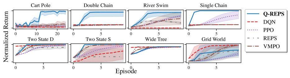
Figure 2: Empirical performance Q-REPS on different benchmarks. The returns are scaled to $[0,1]$ by dividing by the maximum achievable return, with the mean plotted in solid lines and and the shaded area representing one standard deviation.

One important feature of the bound of Theorem 1 is that it shows no direct dependence on the size of the MDP or the dimensionality of the feature map, which can be seen to justify using Q-REPS with general (possibly non-linear) function approximation. Indeed, observe that every MDP can be seen to satisfy Assumption 2 when choosing $\Phi$ as the identity map, and that the logistic Bellman error can be directly written as a function of the Q-functions. Then, Theorem 1 shows that whenever one is able to keep the policy evaluation errors small, convergence to the optimal policy can be guaranteed irrespective of the size of the state space. Among other implications, this suggests that the logistic Bellman error can indeed be a viable objective function for large-scale deep reinforcement learning.

Concentration of the empirical LBE.

We now move on to establishing some important properties of the empirical logistic Bellman error (11). For simplicity, we will assume that the sample transitions are generated in an i.i.d. fashion: each $(X_{k,n},A_{k,n})$ is drawn independently from $\mu_{k}$ and $X_{k,n}^{\prime}$ is drawn independently from $P(\cdot|X_{k,n},A_{k,n})$. Under this condition, the following theorem establishes the connection between the ELBE and the true LBE:

Theorem 2.

Let $\mathcal{Q}=\left\{Q_{\theta}:\left\|Q_{\theta}\right\|_{\infty}\leq B^{\prime}\right\}$ for some $B^{\prime}>0$ and $\Theta$ be the corresponding set of parameter vectors. Furthermore, define $B=1+(1+\gamma)B^{\prime}$, and assume that $\eta B\leq 1$ holds. Then, with probability at least $1-\delta$, the following holds:

$$\sup_{\theta\in\Theta}\left|\widehat{\mathcal{G}}_{k}(\theta)-\mathcal{G}_{k}(\theta)\right|\leq 8\eta B^{2}+56\sqrt{\frac{m\log\bigl{(}(1+4BN)/\delta\bigr{)}}{N}}.$$

In Appendix A.3, we provide a more detailed statement of the theorem that holds for general Q-function classes, as well as the proof. The main feature of this theorem is quantifying the bias of the empirical LBE, showing that it is proportional to the regularization parameter $\eta$, making it possible to tune the parameters of Q-REPS in a way that ensures convergence to the optimal policy.

Q-REPS performance guarantees.

Putting the results from the previous sections together, we obtain the following performance guarantee for Q-REPS:

Corollary 1.

Suppose that Assumptions 1 and 2 hold and that each update Q-REPS is implemented by minimizing the empirical LBE (11) evaluated on $N$ independent sample transitions. Furthermore, suppose that $\left\|Q_{k}^{*}\right\|_{\infty}\leq B$ for all $k$. Then, setting $N=K$ and tuning $\eta$ and $\alpha$ appropriately, Q-REPS is guaranteed to output an $\epsilon$-optimal policy with

$$\epsilon=\widetilde{O}\left(\left(\sqrt{\frac{1}{1-\gamma}}\!+\!B\right)\sqrt{\frac{mC_{\gamma}D(d^{*}\|d_{0})}{K}}\right).$$

Furthermore, for any $\epsilon>0$ and the same choice of $\eta$ and $\alpha$, Q-REPS is guaranteed to output an $\epsilon$-optimal policy after observing $T_{\epsilon}=NK$ transitions with

$$T_{\epsilon}=\widetilde{O}\left(\frac{\left(\left(B^{2}+\frac{1}{1-\gamma}\right)mC_{\gamma}D(d^{*}\|d_{0})\right)^{2}}{\epsilon^{4}}\right).$$

5 EXPERIMENTS

In this section we evaluate Q-REPS empirically. As the algorithm is essentially on-policy, we compare it with: DQN using Polyak averaging and getting new samples at every episode (Mnih et al.,, 2015); PPO as a surrogate of TRPO (Schulman et al.,, 2017); VMPO as the on-policy version of MPO (Song et al.,, 2020); and REPS with parametric policies (Deisenroth et al.,, 2013). The code used for these experiments is available online at https://github.com/sebascuri/qreps.

We evaluate these algorithms in different standard environments which we describe in Appendix B. In all environments we use indicator features, except for Cart-Pole that we use the initialization of a 2-layer ReLU Neural Network as features and optimize the last layer. For all environments but CartPole we run episodes of length 200 and update the policy at the end of each episode. Due to the early-termination of CartPole, we run episodes until termination or length 200 and update the policy after 4 episodes.

In Figure 2 we plot the sample mean and one standard deviation of 50 independent runs of the algorithms (random seeds 0 to 49). In all cases, Q-REPS either outperforms the competing algorithms or is at least comparable them.

6 CONCLUSION

Due to its many favorable properties, we believe that Q-REPS has significant potential to become a state-of-the-art method for reinforcement learning. That said, there is still a lot of room for improvement on both fronts of theoretical guarantees and practical applicability. We outline some challenges for future research and discuss some implications of our results below.

Limitations of our theory.

While our theoretical guarantees have several desirable properties, they also have a number of shortcomings. First, while the error-propagation guarantee of Theorem 1 has no explicit dependence on the number of states, it requires a very restrictive concentrability condition to hold. We believe that this is an artifact of our analysis and expect that it can be removed by a more careful proof technique. Similarly, our Theorem 2 shows that the bias of the straightforward empirical estimator of the LBE can be controlled by the regularization parameter $\eta$, but it comes with the caveat that it requires the condition that the logistic Q-functions be bounded. While we were not able to prove an explicit upper bound on the Q-functions, our extensive supplementary experiments indicate that they are bounded by a constant independent of $\eta$, and we believe that a more sophisticated analysis could formally establish this property. In light of these limitations, we prefer to think of the guarantees of Theorems 1 and 2 as promising initial results, and we leave the important challenge of tightening these guarantees open for future work.

Limitations of our algorithm.

The most important merit of Q-REPS is that it can be implemented without any significant deviation from its theoretical specifications. The most serious implementation issue is that Q-REPS requires sampling from the discounted occupancy measure, which can only be done efficiently when having access to a reset action. This is a common issue of many reinforcement learning algorithms that is often addressed by using samples from the undiscounted state-action distribution. This heuristic often leads to well-performing practical algorithms, but has been long known to suffer from bias issues, as pointed out by Thomas, (2014) and Nota and Thomas, (2020). We expect that this heuristic could help practical implementations of Q-REPS, although it should be applied with caution. Another practical limitation of our algorithm is that it requires storing the cumulative sum of all past Q-functions, which is not feasible without approximations in a deep RL implementation. It is straightforward to address this limitation by adjusting the regularization terms, but it is currently unclear if it is still possible to meaningfully control the error propagation of the resulting variant.

Experience replay and MinMax-Q-REPS.

Interestingly, the saddle-point optimization scheme proposed in Section 3.2 can be seen as a principled form of prioritized experience replay where the samples used for value-function updates are drawn according to some priority criteria (Schaul et al.,, 2016). Indeed, this method maintains a probability distribution over sample transitions that governs the value updates, with the distribution being adjusted after each update according to a rule that is determined by the TD error. Different rules for the priority updates result in different learning dynamics with the best choice potentially depending on the problem instance. In our experiments, we have observed that best-response updates are sometimes overly aggressive, and the incremental updates featured in Algorithm 2 lead to more stable behavior. We leave a formal study of the best practices and uncovering further connections with prioritized experience replay for future research.

The relaxed LP formulation.

Our method is based on a subtle variation on the classic LP formulation of optimal control in MDPs due to Manne, (1960). One key element in our formulation is a linear relaxation of some of the constraints in this LP, which is a technique looking back to a long history: a similar relaxation has been first proposed by Schweitzer and Seidmann, (1985), whose approach was later popularized by the influential work of de Farias and Van Roy, (2003). This latter paper initiated a long line of work studying the properties of solutions to various linearly relaxed versions of the LP, mostly focusing on the quality of value functions extracted from the solutions (see, e.g., Petrik and Zilberstein,, 2009; Desai et al.,, 2012; Lakshminarayanan et al.,, 2018). Another complementary line of work was initiated by Peters et al., (2010), whose main goal was deriving practical RL algorithms from a relaxed LP formulation. Our own work is heavily influenced by this latter line of research, in that our main focus is also on algorithmic aspects. That said, one important result in our paper is providing a sufficient condition for the LP relaxation to yield exact solutions to the original LP: our analysis shows that for factored linear MDPs, the relaxation we propose suffers from no approximation error (cf. Proposition 4). Understanding the approximation errors without this structural assumption is a very exciting question that we plan to address in future work, building on the approximate linear programming literature initiated by de Farias and Van Roy, (2003). Similarly, we expect that our algorithmic techniques can be combined with other, more sophisticated relaxation methods. In light of this discussion, we view our work as a promising step toward bridging the gap between LP-based approximate dynamic-programming approaches and mainstream reinforcement learning.

Acknowledgements

This project has received funding from the European Research Council (ERC) under the European Unions Horizon 2020 research and innovation program grant agreement No 815943. G. Neu was supported by “la Caixa” Banking Foundation through the Junior Leader Postdoctoral Fellowship Programme, a Google Faculty Research Award, and the Bosch AI Young Researcher Award.

Appendix A Omitted proofs

A.1 The proof of Proposition  1

The proof is based on Lagrangian duality: we introduce a set of multipliers $V\in{}^{X}$ and $\theta\in{}^{m}$ for the two sets of constraints and $\rho$ for the normalization constraint of $\mu$, and write the Lagrangian of the constrained optimization problem (9) as

$$\mathcal{L}(\mu,d;V,\theta,\rho)= \left\langle\mu,r\right\rangle+\left\langle V,\gamma P^{\mathsf{\scriptscriptstyle T}}\mu+(1-\gamma)\nu_{0}-E^{\mathsf{\scriptscriptstyle T}}d\right\rangle+\left\langle\theta,\Phi^{\mathsf{\scriptscriptstyle T}}d-\Phi^{\mathsf{\scriptscriptstyle T}}\mu\right\rangle+\rho\left(1-\left\langle\mu,\bm{1}\right\rangle\right)-\frac{1}{\eta}D(\mu\|\mu_{0})-\frac{1}{\alpha}H(d\|d_{0})$$

$$= \left\langle\mu,r+\gamma PV-\Phi\theta-\rho\bm{1}\right\rangle+\left\langle d,\Phi\theta-EV\right\rangle+(1-\gamma)\left\langle\nu_{0},V\right\rangle+\rho-\frac{1}{\eta}D(\mu\|\mu_{0})-\frac{1}{\alpha}H(d\|d_{0})$$

$$= \left\langle\mu,\Delta_{\theta,V}-\rho\bm{1}\right\rangle+\left\langle d,Q_{\theta}-EV\right\rangle+(1-\gamma)\left\langle\nu_{0},V\right\rangle+\rho-\frac{1}{\eta}D(\mu\|\mu_{0})-\frac{1}{\alpha}H(d\|d_{0}),$$ (13)

where we used the notation $Q_{\theta}=\Phi\theta$ and $\Delta_{\theta,V}=r+\gamma PV-Q_{\theta}$ in the last line. Notice that the above is a strictly concave function of $d$ and $\mu$, so its maximum can be found by setting the derivatives with respect to these parameters to zero. In order to do this, we note that

$$\frac{\partial D(\mu\|\mu_{0})}{\partial\mu(x,a)}=\log\mu(x,a)-\log\mu_{0}(x,a)\qquad\mbox{and }\qquad\frac{\partial H(d\|d_{0})}{\partial d(x,a)}=\log\pi_{d}(a|x)-\log\pi_{0}(a|x),$$

where $\pi_{d}(a|x)=d(x,a)/\sum_{a^{\prime}}d(x,a^{\prime})$ and the last expression can be derived by straightforward calculations (see, e.g., Appendix A.4 in Neu et al.,, 2017). This gives the following expressions for the optimal choices of $\mu$ and $d$:

$$\mu^{*}(x,a)=\mu_{0}(x,a)e^{\eta(\Delta_{\theta,V}(x,a)-\rho)}\qquad\mbox{and}\qquad\qquad\pi_{d}^{*}(x,a)=\pi_{0}(a|x)e^{\alpha(Q_{\theta}(x,a)-V(x))}.$$

From the constraint $\sum_{x,a}\mu^{*}(x,a)=1$, we can express the optimal choice of $\rho$ as

$$\rho^{*}=\log\left(\sum_{x,a}{\mu_{0}(x,a)e^{\eta\Delta_{\theta,V}(x,a)}}\right).$$

Similarly, from the constraint $\sum_{a}\pi_{d}^{*}(a|x)=1$, we can express $V$ as a function of $\theta$ for all $x$:

$$V_{\theta}(x)=\frac{1}{\alpha}\log\left(\sum_{a}\pi_{0}(a|x)e^{\alpha Q_{\theta}(x,a)}\right)$$

This implies that $d^{*}$ has the form $d^{*}(x,a)=\nu(x)\pi_{d}^{*}(a|x)$, where $\nu$ is some nonnegative function on the state space. Recalling the definition of $\Delta_{\theta}=r+\gamma PV_{\theta}-Q_{\theta}$ and plugging the above parameters $(\mu^{*},d^{*},\rho^{*},V_{\theta})$ back into the Lagrangian (13) gives

$$\mathcal{G}(\theta)= \mathcal{L}(\mu^{*},d^{*};V_{\theta},\theta,\rho^{*})$$

$$= \sum_{x,a}\left(\mu_{0}(x,a)e^{\eta(\Delta_{\theta}(x,a)-\rho^{*})}(\Delta_{\theta}(x,a)-\rho^{*})+\nu(x)\pi_{0}(a|x)e^{\alpha\left(Q_{\theta}(x,a)-V_{\theta}(x)\right)}\left(Q_{\theta}(x,a)-V_{\theta}(x)\right)\right)$$

$$-\sum_{x,a}\frac{1}{\eta}\left(\mu_{0}(x,a)e^{\eta(\Delta_{\theta}(x,a)-\rho^{*})}\log\frac{\mu_{0}(x,a)e^{\eta(\Delta_{\theta}(x,a)-\rho^{*})}}{\mu_{0}(x,a)}+\mu_{0}(x,a)-\mu_{0}(x,a)e^{\eta(\Delta_{\theta}(x,a)-\rho^{*})}\right)$$

$$-\sum_{x,a}\frac{1}{\alpha}\nu(x)\pi_{0}(a|x)e^{\alpha\left(Q_{\theta}(x,a)-V_{\theta}(x)\right)}\log\frac{\pi_{0}(a|x)e^{\alpha\left(Q_{\theta}(x,a)-V_{\theta}(x)\right)}}{\pi_{0}(a|x)}+(1-\gamma)\left\langle\nu_{0},V\right\rangle+\rho^{*}$$

$$= \sum_{x,a}\left(\mu_{0}(x,a)e^{\eta(\Delta_{\theta}(x,a)-\rho^{*})}(\Delta_{\theta}(x,a)-\rho^{*})+\nu(x)\pi_{0}(a|x)e^{\alpha\left(Q_{\theta}(x,a)-V_{\theta}(x)\right)}\left(Q_{\theta}(x,a)-V_{\theta}(x)\right)\right)$$

$$-\sum_{x,a}\mu_{0}(x,a)e^{\eta(\Delta_{\theta}(x,a)-\rho^{*})}(\Delta_{\theta}(x,a)-\rho^{*})$$

$$-\sum_{x,a}\nu(x)\pi_{0}(a|x)e^{\alpha\left(Q_{\theta}(x,a)-V_{\theta}(x)\right)}\left(Q_{\theta}(x,a)-V_{\theta}(x)\right)+(1-\gamma)\left\langle\nu_{0},V\right\rangle+\rho^{*}$$

$$= (1-\gamma)\left\langle\nu_{0},V\right\rangle+\rho^{*}$$

$$= (1-\gamma)\left\langle\nu_{0},V\right\rangle+\frac{1}{\eta}\log\left(\sum_{x,a}{\mu_{0}(x,a)e^{\eta\Delta_{\theta}(x,a)}}\right).$$

Furthermore, observe that since the parameters were chosen so that all constraints are satisfied, we also have

$$\mathcal{G}(\theta)=\mathcal{L}(\mu^{*},d^{*};V_{\theta},\theta,\rho^{*})=\left\langle\mu^{*},r\right\rangle-\frac{1}{\eta}D(\mu^{*}\|\mu_{0})-\frac{1}{\alpha}H(d^{*}\|d_{0}).$$ (14)

Thus, the solution of the optimization problem (9) can be indeed written as

$$\max_{\mu,d\geq 0}\min_{\theta,V,\rho}\mathcal{L}(\mu,d;V,\theta,\rho)=\min_{\theta,V,\rho}\max_{\mu,d\geq 0}\mathcal{L}(\mu,d;V,\theta,\rho)=\min_{\theta}\mathcal{L}(\mu^{*},d^{*};V_{\theta},\theta,\rho^{*})=\min_{\theta}\mathcal{G}(\theta),$$

which concludes the proof. ∎

A.2 The proof of Theorem 1

The proof of this result is somewhat lengthy and is broken down into a sequence of lemmas and propositions.

Before analyizing the algorithm, we first establish an important realizability property of factored linear MDPs. Precisely, this result will show that, under Assumption 2, the relaxed constraint set $\mathcal{M}_{\Phi}$ matches the set of valid discounted occupancy measures in an appropriate sense, which can be seen as the bare minimum requirement for being able to show convergence to the optimal policy. We refer to this condition as primal realizability, and show that it holds in the following sense:

Proposition 4.

Let $\mathcal{M}_{\Phi}^{\prime}=\left\{d:(\mu,d)\in\mathcal{M}_{\Phi}\right\}$. Then, under Assumption 2, $\mathcal{M}^{*}=\mathcal{M}^{\prime}_{\Phi}$ holds. Furthermore, letting $(\mu^{*},d^{*})=\mathop{\mbox{ arg\,max}}_{(\mu,d)\in\mathcal{M}_{\Phi}}\left\langle\mu,r\right\rangle$, we have $\left\langle d^{*},r\right\rangle=\max_{\mu\in\mathcal{M}^{*}}\left\langle\mu,r\right\rangle$.

Proof.

It is easy to see that $\mathcal{M}^{*}\subseteq\mathcal{M}_{\Phi}^{\prime}$: for any $\mu\in\mathcal{M}^{*}$, we can choose $d=\mu$ and directly verify that all constraints of (9) are satisfied. For proving the other direction, it is helpful to define the operator $M$ through its action $Mv=\sum_{x}\omega(x)v(x)$ for any $v\in{}^{\mathcal{X}}$, so that the condition of Assumption 2 can be expressed as $P=\Phi M$ and $r=\Phi\vartheta$. Then, for any $(\mu,d)\in\mathcal{M}_{\Phi}$, we write

$$E^{\mathsf{\scriptscriptstyle T}}d =\gamma P^{\mathsf{\scriptscriptstyle T}}\mu+(1-\gamma)\nu_{0}=\gamma M^{\mathsf{\scriptscriptstyle T}}\Phi^{\mathsf{\scriptscriptstyle T}}\mu+(1-\gamma)\nu_{0}$$

$$=\gamma M^{\mathsf{\scriptscriptstyle T}}\Phi^{\mathsf{\scriptscriptstyle T}}d+(1-\gamma)\nu_{0}=\gamma P^{\mathsf{\scriptscriptstyle T}}d+(1-\gamma)\nu_{0}.$$

Combined with the fact that $d$ is non-negative, this implies that $d\in\mathcal{M}^{*}$ and thus that $\mathcal{M}_{\Phi}^{\prime}\subseteq\mathcal{M}^{*}$. Together with the previous argument, this shows that $\mathcal{M}^{*}=\mathcal{M}_{\Phi}^{\prime}$ indeed holds. For proving the second statement, we use the assumption on $r$ to write $\left\langle\mu,r\right\rangle=\left\langle\Phi^{\mathsf{\scriptscriptstyle T}}\mu,\Phi r\right\rangle=\left\langle\Phi^{\mathsf{\scriptscriptstyle T}}d,\Phi r\right\rangle=\left\langle d,r\right\rangle$ for any feasible $(\mu,d)$. Using this fact for the maximizer $d^{*}$ implies $\left\langle d^{*},r\right\rangle=\max_{d\in\mathcal{M}^{\prime}_{\Phi}}\left\langle d,r\right\rangle=\max_{\mu\in\mathcal{M}^{*}}\left\langle\mu,r\right\rangle$, which concludes the proof. ∎

We can now turn to the analysis of Q-REPS. We first introduce some useful notation and outline the main challenges faced in the proof. We start by defining the action-value functions $Q_{k}=\Phi\theta_{k}$ and $Q_{k}^{*}=\Phi\theta_{k}^{*}$, the state-action distributions

$$\widetilde{\mu}_{k}(x,a)=\mu_{k-1}(x,a)e^{\eta\left(\Delta_{\theta_{k}}(x,a)-\rho_{k}\right)}\qquad\mbox{and}\qquad\mu_{k}^{*}(x,a)=\mu_{k-1}(x,a)e^{\eta\left(\Delta_{\theta_{k}^{*}}(x,a)-\rho_{k}^{*}\right)},$$

for appropriately defined normalization constants $\rho_{k}$ and $\rho_{k}^{*}$ and the policies

$$\pi_{k}(a|x)=\pi_{k-1}(a|x)e^{\alpha\left(Q_{\theta_{k}}(x,a)-V_{\theta_{k}}(x)\right)}\qquad\mbox{and}\qquad\pi_{k}^{*}(a|x)=\pi_{k-1}(a|x)e^{\alpha\left(Q_{\theta_{k}^{*}}(x,a)-V_{\theta_{k}^{*}}(x)\right)}.$$

A crucial challenge we have to address in the analysis is that, since $\theta_{k}$ is not the exact minimizer of $\mathcal{G}_{k}$, the state-action distribution $\widetilde{\mu}_{k}$ is not a valid occupancy measure. In order to prove meaningful guarantees about the performance of the algorithm, we need to consider the actual occupancy measure induced by policy $\pi_{k}$. We denote this occupancy measure as $d_{k}$ and define it for all $x,a$ as

$$d_{k}(x,a)=(1-\gamma)\mathbb{E}_{\pi_{k}}\left[\sum_{t=0}^{\infty}\gamma^{t}\mathbb{I}_{\left\{(x_{t},a_{t})=(x,a)\right\}}\right],$$

where the notation emphasizes that the actions are generated by policy $\pi_{k}$. A major part of the proof is dedicated to accounting for the discrepancy between $\mu_{k}$ and the ideal updates $\mu_{k}^{*}$. During the proof, we will often factorize occupancy measures as $d(x,a)=\nu(x)\pi(a|x)$, where $\nu$ is the discounted state-occupancy measure induced by $\pi$. In particular, we will use the notations

$$d_{k}(x,a)=\nu_{k}(x)\pi_{k}(a|x)\qquad\mbox{and}\qquad d_{k}^{*}(x,a)=\nu_{k}^{*}(x)\pi_{k}^{*}(a|x),$$

to refer to the state-action occupancy measures respectively induced by $\pi_{k}$ and $\pi^{*}_{k}$.

Our first lemma presents an important technical result that relates the suboptimality gap $\varepsilon_{k}$ to the divergence between the ideal and realized updates.

Lemma 1.

$\varepsilon_{k}=\frac{D(\mu_{k}^{*}\|\widetilde{\mu}_{k})}{\eta}+\frac{H(d_{k}^{*}\|d_{k})}{\alpha}$.

Notably, this result does not require any of Assumptions 1 or 2, as its proof only uses the properties of the optimization problem (9).

Proof.

The proof uses the feasibility of $(\mu_{k}^{*},d_{k}^{*})$ that follows from their definition. We start by observing that

$$D(\mu_{k}^{*}\|\widetilde{\mu}_{k}) =\sum_{x,a}\mu_{k}^{*}(x,a)\log\frac{\mu_{k}^{*}(x,a)}{\widetilde{\mu}_{k}(x,a)}$$

$$=\eta\bigl{\langle}\mu_{k}^{*},r+\gamma PV_{k}^{*}-Q_{k}^{*}-\rho_{k}^{*}\bm{1}-r-\gamma PV_{k}+Q_{k}+\rho_{k}\bm{1}\bigr{\rangle}$$

$$=\eta\bigl{\langle}d_{k}^{*},EV_{k}^{*}-EV_{k}\bigr{\rangle}+\eta\left\langle\Phi^{\mathsf{\scriptscriptstyle T}}\mu_{k}^{*},\theta_{k}-\theta_{k}^{*}\right\rangle+\eta(\rho_{k}+(1-\gamma)\left\langle\nu_{0},V_{k}\right\rangle-\rho_{k}^{*}-(1-\gamma)\left\langle\nu_{0},V_{k}^{*}\right\rangle)$$

(using $$d_{k}^{*}=\gamma P^{\mathsf{\scriptscriptstyle T}}\mu_{k}^{*}+(1-\gamma)\nu_{0} Q_{k}-Q_{k}^{*}=\Phi(\theta_{k}-\theta^{*}_{k})$$ and )

$$=\eta\bigl{\langle}d_{k}^{*},EV_{k}^{*}-EV_{k}\bigr{\rangle}+\eta\left\langle\Phi^{\mathsf{\scriptscriptstyle T}}d_{k}^{*},\theta_{k}-\theta_{k}^{*}\right\rangle+\eta(\mathcal{G}_{k}(\theta_{k})-\mathcal{G}_{k}(\theta_{k}^{*}))$$

(using $$\Phi^{\mathsf{\scriptscriptstyle T}}d_{k}^{*}=\Phi^{\mathsf{\scriptscriptstyle T}}\mu_{k}^{*} \mathcal{G}_{k}$$ and the form of )

$$=\eta\bigl{\langle}d_{k}^{*},EV_{k}^{*}-Q_{k}^{*}-EV_{k}+Q_{k}\bigr{\rangle}+\eta(\mathcal{G}_{k}(\theta_{k})-\mathcal{G}_{k}(\theta_{k}^{*})).$$

On the other hand, we have

$$H(d_{k}^{*}\|d_{k}) =\sum_{x,a}d_{k}^{*}(x,a)\log\frac{\pi_{k}^{*}(a|x)}{\pi_{k}(a|x)}=\alpha\left\langle d_{k}^{*},Q_{k}^{*}-EV_{k}^{*}-Q_{k}+EV_{k}\right\rangle.$$

Putting the two equalities together, we get

$$\frac{D(\mu_{k}^{*}\|\widetilde{\mu}_{k})}{\eta}+\frac{H(d_{k}^{*}\|d_{k})}{\alpha}=\mathcal{G}_{k}(V_{k})-\mathcal{G}_{k}(V_{k}^{*})$$

as required. ∎

The next result shows that, as a consequence of the above property, the realized occupancy measure $d_{k}$ will be close to the ideal one, $d_{k}^{*}$. The proof only uses Assumption 2 to make sure that $d_{k}^{*}$ is a valid occupancy measure.

Lemma 2.

Suppose that Assumption 2 holds. Then, $D\left(d_{k}^{*}\middle\|d_{k}\right)\leq\frac{H\left(d_{k}^{*}\middle\|d_{k}\right)}{1-\gamma}.$

Proof.

The proof follows from direct calculations and exploiting several properties of the relative entropy:

$$D\left(d_{k}^{*}\middle\|d_{k}\right) =D\left(\nu_{k}^{*}\middle\|\nu_{k}\right)+H\left(d_{k}^{*}\middle\|d_{k}\right)$$

(by the chain rule of the relative entropy)

$$=D\left((1-\gamma)\nu_{0}+\gamma P^{\mathsf{\scriptscriptstyle T}}d_{k}^{*}\middle\|(1-\gamma)\nu_{0}+\gamma P^{\mathsf{\scriptscriptstyle T}}\mu_{k}\right)+H\left(d_{k}^{*}\middle\|d_{k}\right)$$

(using that $$d_{k}^{*} d_{k}$$ and are valid occupancy measures)

$$\leq(1-\gamma)D\left(\nu_{0}\middle\|\nu_{0}\right)+\gamma D\left(P^{\mathsf{\scriptscriptstyle T}}d_{k}^{*}\middle\|P^{\mathsf{\scriptscriptstyle T}}d_{k}\right)+H\left(d_{k}^{*}\middle\|d_{k}\right)$$

(using the joint convexity of the relative entropy)

$$\leq\gamma D\left(d_{k}^{*}\middle\|\mu_{k}\right)+H\left(d_{k}^{*}\middle\|d_{k}\right),$$

where the final step follows from the using information-processing inequality for the relative entropy. Reordering the terms concludes the proof. ∎

Armed with the above two lemmas, we are now ready to present the proof of Theorem 1.

Proof of Theorem 1.

The proof is based on direct calculations inspired by the classical mirror descent analysis. We let $d^{*}=\mathop{\mbox{ arg\,max}}_{d\in\mathcal{M}^{*}}\left\langle d,r\right\rangle$ and $\mu^{*}$ be any state-action distribution satisfying $(\mu^{*},d^{*})\in\mathcal{M}_{\Phi}$. We first express the divergence between the comparator $\mu^{*}$ and the unprojected iterate $\widetilde{\mu}_{k}$:

$$D(\mu^{*}\|\widetilde{\mu}_{k}) =\sum_{x,a}\mu^{*}(x,a)\log\frac{\mu^{*}(x,a)}{\widetilde{\mu}_{k}(x,a)}=\sum_{x,a}\mu^{*}(x,a)\log\frac{\mu(x,a)}{d_{k-1}(x,a)}-\sum_{x,a}\mu^{*}(x,a)\log\frac{\widetilde{\mu}_{k}(x,a)}{d_{k-1}(x,a)}$$

$$=D(\mu^{*}\|d_{k-1})-\eta\left\langle\mu^{*},r+\gamma PV_{k}-Q_{k}\right\rangle+\eta\rho_{k}$$

$$=D(\mu^{*}\|d_{k-1})-\eta\left\langle\mu^{*},r-\Phi\theta_{k}\right\rangle+\eta\left\langle d^{*},EV_{k}\right\rangle+\eta\bigl{(}\rho_{k}+(1-\gamma)\left\langle\nu_{0},V_{k}\right\rangle\bigr{)}$$

(using $$d^{*}=\gamma P^{\mathsf{\scriptscriptstyle T}}\mu^{*}+(1-\gamma)\nu_{0} Q_{k}=\Phi\theta_{k}$$ and )

$$=D(\mu^{*}\|d_{k-1})-\eta\left\langle\mu^{*},r\right\rangle+\eta\left\langle d^{*},EV_{k}-\Phi\theta_{k}\right\rangle+\eta\mathcal{G}_{k}(\theta_{k})$$

(using $$\Phi^{\mathsf{\scriptscriptstyle T}}d^{*}=\Phi^{\mathsf{\scriptscriptstyle T}}\mu^{*} \mathcal{G}_{k}$$ and the form of )

$$\leq D(\mu^{*}\|d_{k-1})-\eta\left\langle\mu^{*},r\right\rangle+\eta\left\langle d^{*},EV_{k}-\Phi\theta_{k}\right\rangle+\eta\mathcal{G}_{k}(\theta_{k}^{*})+\eta\varepsilon_{k}$$

(using the suboptimality guarantee of $$\theta_{k}$$)

$$\leq D(\mu^{*}\|d_{k-1})-\eta\left\langle\mu^{*},r\right\rangle+\eta\left\langle d^{*},EV_{k}-\Phi\theta_{k}\right\rangle+\eta\left\langle\mu_{k}^{*},r\right\rangle-D(\mu_{k}^{*}\|d_{k-1})-\frac{\eta H(d^{*}_{k}\|d_{k-1})}{\alpha}+\eta\varepsilon_{k}$$

(using the dual form (14) of $$\mathcal{G}_{k}(\theta_{k})$$)

$$\leq D(\mu^{*}\|d_{k-1})-\eta\left\langle\mu^{*},r\right\rangle+\eta\left\langle d^{*},EV_{k}-\Phi\theta_{k}\right\rangle+\eta\left\langle d_{k},r\right\rangle+\eta\left\langle d_{k}^{*}-d_{k},r\right\rangle+\eta\varepsilon_{k}$$

(using that $$\left\langle d_{k}^{*},r\right\rangle=\left\langle\mu_{k}^{*},r\right\rangle$$ by Proposition 4)

$$\leq D(\mu^{*}\|d_{k-1})-\eta\left\langle\mu^{*},r\right\rangle+\eta\left\langle d^{*},EV_{k}-\Phi\theta_{k}\right\rangle+\eta\left\langle d_{k},r\right\rangle+\eta\left\|d_{k}^{*}-d_{k}\right\|_{1}+\eta\varepsilon_{k},$$

where we used $\left\|r\right\|_{\infty}\leq 1$ in the last step. After reordering and noticing that $\left\langle\mu^{*},r\right\rangle=\left\langle d^{*},r\right\rangle$, we obtain

$$\left\langle d^{*}-d_{k},r\right\rangle\leq\frac{D(\mu^{*}\|d_{k-1})-D(\mu^{*}\|\widetilde{\mu}_{k})}{\eta}+\left\langle d^{*},EV_{k}-Q_{k}\right\rangle+\eta\left\|d_{k}^{*}-d_{k}\right\|_{1}+\varepsilon_{k}.$$

Furthermore, we have

$$H(d^{*}\|d_{k}) =\sum_{x,a}d^{*}(x,a)\log\frac{\pi^{*}(a|x)}{\pi_{k}(a|x)}=\sum_{x,a}d^{*}(x,a)\log\frac{\pi^{*}(a|x)}{\pi_{k-1}(a|x)}-\sum_{x,a}\mu(x,a)\log\frac{\pi_{k}(a|x)}{\pi_{k-1}(a|x)}$$

$$=H(d^{*}\|d_{k-1})-\alpha\left\langle d^{*},Q_{k}-EV_{k}\right\rangle.$$

Plugging this equality back into the previous bound, we finally obtain

$$\left\langle d^{*}-d_{k},r\right\rangle\leq\frac{D(\mu^{*}\|d_{k-1})-D(\mu^{*}\|\widetilde{\mu}_{k})}{\eta}+\frac{H(d^{*}\|d_{k-1})-H(d^{*}\|d_{k})}{\alpha}+\left\|d_{k}^{*}-d_{k}\right\|_{1}+\varepsilon_{k}$$

$$\qquad=\frac{D(\mu^{*}\|d_{k})-D(\mu^{*}\|\widetilde{\mu}_{k})}{\eta}+\frac{D(\mu^{*}\|d_{k-1})-D(\mu^{*}\|d_{k})}{\eta}+\frac{H(d^{*}\|d_{k-1})-H(d^{*}\|d_{k})}{\alpha}+\left\|d_{k}^{*}-d_{k}\right\|_{1}+\varepsilon_{k}.$$

Summing up for all $k$ and omitting some nonpositive terms, we obtain

$$\sum_{k=1}^{K}\left\langle d^{*}-d_{k},r\right\rangle\leq\frac{D(\mu^{*}\|d_{0})}{\eta}+\frac{H(d^{*}\|d_{0})}{\alpha}+\sum_{k=1}^{K}\left(\frac{D(\mu^{*}\|d_{k})-D(\mu^{*}\|\widetilde{\mu}_{k})}{\eta}+\left\|d_{k}^{*}-d_{k}\right\|_{1}+\varepsilon_{k}\right)$$ (15)

Combining Lemma 2 with Pinsker’s inequality, we can bound

$$\left\|d_{k}^{*}-d_{k}\right\|_{1}\leq\sqrt{2D(d_{k}^{*}\|d_{k})}\leq\sqrt{\frac{2H(d_{k}^{*}\|d_{k})}{1-\gamma}}\leq\sqrt{\frac{2\alpha\varepsilon_{k}}{1-\gamma}},$$

where in the last step we also used Lemma 1 that implies $H(d_{k}^{*}\|\widetilde{d}_{k})\leq\alpha\varepsilon_{k}$. Thus, the remaining challenge is to bound the terms $D(\mu^{*}\|d_{k})-D(\mu^{*}\|\widetilde{\mu}_{k})$. In order to do this, let us introduce the Bregman projection of $\widetilde{\nu}_{k}$ to the space of occupancy measures, $\widetilde{\nu}_{k}^{*}=\mathop{\mbox{ arg\,min}}_{\nu\in\Delta_{\gamma}(\mathcal{X})}D(\nu\|\widetilde{\nu}_{k})$. Then, we can write

$$D(\mu^{*}\|d_{k})-D(\mu^{*}\|\widetilde{\mu}_{k})= D(\nu^{*}\|\nu_{k})-D(\nu^{*}\|\widetilde{\nu}_{k})$$

$$= D(\nu^{*}\|\nu_{k})-D(\nu^{*}\|\widetilde{\nu}_{k}^{*})+D(\nu^{*}\|\widetilde{\nu}_{k}^{*})-D(\nu^{*}\|\widetilde{\nu}_{k})$$

$$\leq D(\nu^{*}\|\nu_{k})-D(\nu^{*}\|\widetilde{\nu}_{k}^{*})-D(\widetilde{\nu}_{k}^{*}\|\widetilde{\nu}_{k})\leq D(\nu^{*}\|\nu_{k})-D(\nu^{*}\|\widetilde{\nu}_{k}^{*}),$$

where the first inequality is the generalized Pythagorean inequality that uses the fact that $\widetilde{\nu}_{k}^{*}$ is the Bregman projection of $\widetilde{\nu}_{k}$ (cf. Lemma 11.3 in Cesa-Bianchi and Lugosi,, 2006). By using the chain rule of the relative entropy and appealing to Lemma 2, we have

$$D(\nu_{k}^{*}\|\widetilde{\nu}_{k})=D(\mu_{k}^{*}\|\widetilde{\mu}_{k})-H(\mu_{k}^{*}\|\widetilde{\mu}_{k})\leq D(\mu_{k}^{*}\|\widetilde{\mu}_{k})\leq\eta\varepsilon_{k},$$

which implies $D(\widetilde{\nu}_{k}^{*}\|\widetilde{\nu}_{k})\leq D(\nu_{k}^{*}\|\widetilde{\nu}_{k})\leq\eta\varepsilon_{k}$ due to the properties of the projected point $\widetilde{\nu}_{k}^{*}$. To proceed, we use the inequality $\log(u)\leq u-1$ that holds for all $u>-1$ to write

$$D(\nu^{*}\|\nu_{k})-D(\nu^{*}\|\widetilde{\nu}_{k}^{*}) =\sum_{x}\nu^{*}(x)\log\frac{\nu_{k}(x)}{\widetilde{\nu}_{k}^{*}(x)}\leq\sum_{x}\nu^{*}(x)\left(\frac{\nu_{k}(x)}{\widetilde{\nu}_{k}^{*}(x)}-1\right)=\sum_{x}\frac{\nu^{*}(x)}{\widetilde{\nu}_{k}^{*}(x)}\left(\nu_{k}(x)-\widetilde{\nu}_{k}^{*}(x)\right)$$

$$\leq\sum_{x}\frac{\nu^{*}(x)}{\widetilde{\nu}_{k}^{*}(x)}\left|\nu_{k}(x)-\widetilde{\nu}_{k}^{*}(x)\right|\leq\max_{x^{\prime}}\frac{\nu^{*}(x^{\prime})}{\widetilde{\nu}_{k}^{*}(x^{\prime})}\sum_{x}\left|\nu_{k}(x)-\widetilde{\nu}_{k}^{*}(x)\right|$$

$$\leq C_{\gamma}\left\|\nu_{k}-\widetilde{\nu}_{k}^{*}\right\|_{1}\leq C_{\gamma}\left(\left\|\nu_{k}-\nu_{k}^{*}\right\|_{1}+\left\|\nu_{k}^{*}-\widetilde{\nu}_{k}\right\|_{1}+\left\|\widetilde{\nu}_{k}-\widetilde{\nu}_{k}^{*}\right\|_{1}\right)$$

(by Assumption 1 and the triangle inequality)

$$\leq C_{\gamma}\left(\sqrt{\frac{2H(d_{k}^{*}\|d_{k})}{1-\gamma}}+\sqrt{2D(\nu_{k}^{*}\|\widetilde{\nu}_{k})}+\sqrt{2D(\widetilde{\nu}_{k}^{*}\|\widetilde{\nu}_{k})}\right)$$

(by applying Pinsker’s inequality twice and invoking Lemma 2)

$$\leq C_{\gamma}\sqrt{\frac{2\alpha\varepsilon_{k}}{1-\gamma}}+C_{\gamma}\sqrt{8\eta\varepsilon_{k}}.$$

Plugging all bounds back into the bound of Equation (15) and using that $C_{\gamma}\geq 1$, we obtain

$$\sum_{k=1}^{K}\left\langle d^{*}-d_{k},r\right\rangle\leq\frac{D(\mu^{*}\|d_{0})}{\eta}+\frac{H(d^{*}\|d_{0})}{\alpha}+C_{\gamma}\left(\sqrt{\frac{8\alpha}{1-\gamma}}+\sqrt{8\eta}\right)\sum_{k=1}^{K}\sqrt{\varepsilon_{k}}+\sum_{k=1}^{K}\varepsilon_{k},$$

thus concluding the proof of the theorem. ∎

A.3 The proof of Theorem 2

We will prove the following, more general version of the theorem below:

Theorem 2.

(General statement) Let $\mathcal{Q}=\left\{Q_{\theta}:\left\|Q_{\theta}\right\|_{\infty}\leq B^{\prime}\right\}$ for some $B^{\prime}>0$ and $\Theta$ be the corresponding set of parameter vectors, and let $\mathcal{N}_{\mathcal{Q},\epsilon}$ be the $\epsilon$-covering number of $\mathcal{Q}$ with respect to the $\ell_{\infty}$ norm. Furthermore, define $B=1+(1+\gamma)B^{\prime}$, and assume that $\eta B\leq 1$ holds. Then, with probability at least $1-\delta$, the following holds:

$$\sup_{\theta\in\Theta}\left|\widehat{\mathcal{G}}_{k}(\theta)-\mathcal{G}_{k}(\theta)\right|\leq 8\eta B^{2}+56\sqrt{\frac{\log(2\mathcal{N}_{\mathcal{Q},1/\sqrt{N}}/\delta)}{N}}.$$

The proof of the version stated in the main body of the paper follows from bounding the covering number of our linear Q-function class as $\mathcal{N}_{\mathcal{Q},\epsilon}\leq(1+4B/\epsilon)^{m}$.

Proof.

We first prove a concentration bound for a fixed $\theta$ and then provide a uniform guarantee through a covering argument.

For the first part, let us fix a confidence level $\delta^{\prime}>0$ and an arbitrary $\theta$, and define the shorthand notation $\widehat{S}_{n}=\widehat{\Delta}_{\theta}(X_{k,n},A_{k,n},X^{\prime}_{k,n})$ and $S_{n}=\Delta_{\theta}(X_{k,n},A_{k,n})$. Note that, by definition, these random variables are bounded in the interval $[-(\gamma+1)B^{\prime},1+(\gamma+1)B^{\prime}]\subset[-B,B]$. Furthermore, let us define the notation $\mathbb{E}_{X^{\prime}}\left[\cdot\right]=\mathbb{E}\left[\cdot\left|\left\{X_{k,n},A_{k,n}\right\}_{n=1}^{N}\right.\right]$ and let

$$W=\frac{1}{N}\sum_{n=1}^{N}e^{\eta\widehat{S}_{n}}\qquad\mbox{and}\qquad\overline{W}=\frac{1}{N}\sum_{n=1}^{N}e^{\eta S_{n}}.$$

We start by observing that, by Jensen’s inequality, we obviously have $\mathbb{E}_{X^{\prime}}\left[W\right]\leq\overline{W}$. Furthermore, by using the inequality $e^{u}\leq 1+u+u^{2}$ that holds for all $u\leq 1$, we can further write

$$\overline{W} \leq\frac{1}{N}\sum_{n=1}^{N}\left(1+\eta S_{n}+\eta^{2}S_{n}^{2}\right)\leq\mathbb{E}_{X^{\prime}}\left[\frac{1}{N}\sum_{n=1}^{N}\left(1+\eta\widehat{S}_{n}\right)\right]+\eta^{2}S_{n}^{2}$$

$$\leq\mathbb{E}_{X^{\prime}}\left[\frac{1}{N}\sum_{n=1}^{N}e^{\eta\widehat{S}_{n}}\right]+\eta^{2}S_{n}^{2}=\mathbb{E}_{X^{\prime}}\left[W\right]+\eta^{2}B^{2},$$

where in the last line we used the inequality $1+u\leq e^{u}$ that holds for all $u$ and our upper bound on $\widehat{S}_{n}$. Thus, taking expectations with respect to $X^{\prime}$, we get

$$\mathbb{E}\left[W\right]\leq\mathbb{E}\left[\overline{W}\right]\leq\mathbb{E}\left[W\right]+\eta^{2}B^{2}.$$ (16)

To proceed, we define the function

$$f(s_{1},s_{2},\dots,s_{N})=\frac{1}{N}\sum_{n=1}^{N}e^{\eta s_{n}}$$

and notice that it satisfies the bounded-differences property

$$f(s_{1},s_{2},\dots,s_{n},\dots,s_{N})-f(s_{1},s_{2},\dots,s_{n}^{\prime},\dots,s_{N})=\frac{1}{N}\left(e^{\eta s_{n}}-e^{\eta s_{n}^{\prime}}\right)\leq\frac{\eta e^{2\eta B}}{N}.$$

Here, the last step follows from Taylor’s theorem that implies that there exists a $\chi\in(0,1)$ such that

$$e^{\eta s_{n}^{\prime}}=e^{\eta s_{n}}+\eta e^{\eta\chi\left(s_{n}^{\prime}-s_{n}\right)}$$

holds, so that $e^{\eta s_{n}^{\prime}}-e^{\eta s_{n}}=\eta e^{\eta\chi\left(s_{n}^{\prime}-s_{n}\right)}\leq\eta e^{2\eta B}$, where we used the assumption that $|s_{n}-s_{n}^{\prime}|\leq 2B$ in the last step. Notice that our assumption $\eta B\leq 1$ further implies that $e^{2\eta B}\leq e^{2}$. Thus, also noticing that $W=f(S_{1},\dots,S_{N})$, we can apply McDiarmid’s inequality that to show that the following holds with probability at least $1-\delta^{\prime}$:

$$|W-\mathbb{E}\left[W\right]|\leq\eta e^{2}\sqrt{\frac{\log(2/\delta^{\prime})}{N}}.$$ (17)

Now, let us observe that the difference between the LBE and its empirical counterpart can be written as

$$\widehat{\mathcal{G}}_{k}(\theta)-\mathcal{G}_{k}(\theta)=\frac{1}{\eta}\log\left(W\right)-\frac{1}{\eta}\log\left(\mathbb{E}\left[\overline{W}\right]\right)=\frac{1}{\eta}\log\left(\frac{W}{\mathbb{E}\left[\overline{W}\right]}\right).$$

Thus, by combining Equations (16) and (17), we obtain that

$$\widehat{\mathcal{G}}_{k}(\theta)-\mathcal{G}_{k}(\theta) =\frac{1}{\eta}\log\left(1+\frac{W-\mathbb{E}\left[\overline{W}\right]}{\mathbb{E}\left[\overline{W}\right]}\right)\leq\frac{1}{\eta}\log\left(1+\frac{W-\mathbb{E}\left[W\right]}{\mathbb{E}\left[\overline{W}\right]}\right)$$

$$\leq\frac{W-\mathbb{E}\left[W\right]}{\eta\mathbb{E}\left[\overline{W}\right]}\leq e^{4}\sqrt{\frac{\log(2/\delta^{\prime})}{N}},$$

where we used the inequality $\log(1+u)\leq u$ that holds for $u>-1$ and our assumption on $\eta$ that implies $\overline{W}\geq e^{-2}$. Similarly, we can show

$$\mathcal{G}_{k}(\theta)-\widehat{\mathcal{G}}_{k}(\theta) =\frac{1}{\eta}\log\left(1+\frac{\mathbb{E}\left[\overline{W}\right]-W}{W}\right)\leq\frac{1}{\eta}\log\left(1+\frac{\mathbb{E}\left[W\right]-W+\eta^{2}B^{2}}{W}\right)$$

$$\leq\frac{\mathbb{E}\left[W\right]-W+\eta^{2}B^{2}}{\eta W}\leq e^{4}\sqrt{\frac{\log(2/\delta^{\prime})}{N}}+\eta e^{2}B^{2},$$

This concludes the proof of the concentration result for a fixed $\theta$.

In order to prove a bound that holds uniformly for all values of $\theta$, we will consider a covering of the space of Q functions $Q_{\theta}$ bounded in terms of the supremum norm $\mathcal{Q}=\left\{Q_{\theta}:\,\theta\in{}^{m},\left\|Q_{\theta}\right\|_{\infty}\leq B\right\}$. The corresponding set of parameters will be denoted as $\Theta$. To define the covering, we fix an $\epsilon>0$ and consider a set $\mathcal{C}_{\mathcal{Q},\epsilon}\subset\mathcal{Q}$ of minimum cardinality, such that for all $Q_{\theta}\in\mathcal{Q}$, there exists a $\theta^{\prime}\in\mathcal{C}_{\mathcal{Q},\epsilon}$ satisfying $|\mathcal{G}_{k}(\theta)-\mathcal{G}_{k}(\theta^{\prime})|\leq\epsilon$. Defining the covering number $\mathcal{N}_{\mathcal{Q},\epsilon}=\left|\mathcal{C}_{\mathcal{Q},\epsilon}\right|$ and $\epsilon=1/\sqrt{N}$, we can combine the above concentration result with a union bound over the covering $\mathcal{C}_{\mathcal{Q},\epsilon}$ to get that

$$\sup_{\theta\in\Theta}\left|\mathcal{G}_{k}(\theta)-\widehat{\mathcal{G}}_{k}(\theta)\right|\leq\left(e^{4}+1\right)\sqrt{\frac{\log(2\mathcal{N}_{\mathcal{Q},\epsilon}/\delta)}{N}}+\eta e^{2}B^{2}$$

holds with probability at least $1-\delta$. Upper-bounding the constants $e^{2}<8$ and $e^{4}+1<56$ concludes the proof. ∎

A.4 The proof of Proposition 3

For each $i$, the partial derivatives of $S(\theta,z)$ with respect to $\theta_{i}$ can written as

$$\frac{\partial S(\theta,z)}{\partial\theta_{i}}\sum_{n}z(n)\frac{\partial\widehat{\Delta}(X_{k,n},A_{k,n},X_{k,n}^{\prime})}{\partial\theta_{i}}+\sum_{x,y,a}(1-\gamma)\nu_{0}(x)\frac{\partial V_{\theta}(x)}{\partial Q_{\theta}(y,a)}\frac{\partial Q_{\theta}(y,a)}{\partial\theta_{i}}.$$ (18)

Computing the derivatives

$$\frac{\partial V_{\theta}(x)}{\partial Q_{\theta}(y,a)}=\mathbb{I}_{\left\{x=y\right\}}\frac{\pi_{k}(a|x)e^{\alpha Q_{\theta}(x,a)}}{\sum_{a^{\prime}}\pi_{k}(a^{\prime}|x)e^{\alpha Q_{\theta}(x,a^{\prime})}}=\mathbb{I}_{\left\{x=y\right\}}\pi_{k,\theta}(a|x)$$

and

$$\frac{\partial\widehat{\Delta}(X_{k,n},A_{k,n},X^{\prime}_{k,n})}{\partial\theta_{i}}= \gamma\sum_{x,a}\frac{\partial V_{\theta}(X^{\prime}_{k,n})}{\partial Q_{\theta}(x,a)}\frac{\partial Q_{\theta}(x,a)}{\partial\theta_{i}}-\frac{\partial Q_{\theta}(X_{k,n},A_{k,n})}{\partial\theta_{i}}$$

$$= \gamma\sum_{a}\pi_{k,\theta}(X^{\prime}_{k,n},a)\varphi_{i}(X^{\prime}_{k,n},a)-\varphi_{i}(X_{k,n},A_{k,n})$$

and plugging them back in Equation (18), we get

$$\nabla_{\theta}S(\theta,z)=\sum_{n=1}^{N}z(n)\left(\gamma\sum_{a}\pi_{k,\theta}(a|X_{k,n})\varphi(X_{k,n}^{\prime},a)-\varphi(X_{k,n},A_{k,n})\right)+\sum_{x,a}(1-\gamma)\nu_{0}(x)\pi_{k,\theta}(a|x)\varphi(x,a).$$

The statement of the proposition can now be directly verified using the definitions of $X,A,X^{\prime}$ and $\overline{X},\overline{A}$. ∎

Appendix B Experimental details and further experiments

Environment description.

We use Double-chain and Single-Chain from Furmston and Barber, (2010), River Swim from Strehl and Littman, (2008), WideTree from Ayoub et al., (2020), CartPole from Brockman et al., (2016), Two-State Deterministic from Bagnell and Schneider, (2003), windy-grid world from Sutton and Barto, (2018), and a new Two-State Stochastic that we present in Figure 3.

Code environment.

We use the open-source implementation of these algorithms from Curi, (2020) which is based on PyTorch (Paszke et al.,, 2017).

Hyperparameters.

In Table 1 we show the hyperparameters we use for each environment. We fix the regularization parameters as $\eta=\alpha$ and set them so that $1/\eta$ matches the average optimal returns in each game. As optimizers for the player controlling the $\theta$ parameters in MinMax-Q-REPS (the learner), we use SGD (Robbins and Monro,, 1951) and in CartPole we use Adam (Kingma and Ba,, 2014). For the player controlling the distributions $z$ (the sampler), we use the exponentited gradient (EG) update explained in the main text as the default choice, and use the best response (BR) for CartPole:

$$z_{k,\tau+1}(n)\propto e^{\eta\widehat{\Delta}_{k,\tau}(\xi_{k,n})}.$$

The learning rates $\beta$ and $\beta^{\prime}$ were picked as the largest values that resulted in stable optimization performance.

Features for CartPole

We initialize a two-layer neural network with a hidden layer of 200 units and ReLU activations, and use the default initialization from PyTorch. We freeze the first layer and use the outputs of the activations as state features $\phi^{\prime}:\mathcal{X}\rightarrow{}^{200}$. To account for early termination, we multiply each of the features with an indicator feature $\delta(x)$ that takes the value $1$ if the transition is valid and $0$ if the next transition terminates. The final state features are given by the product $\phi(x)=\phi^{\prime}(x)\delta(x)\in\mathbb{R}^{200}_{\geq 0}$. Finally, we define state-action features $\varphi:\mathcal{X}\times\mathcal{A}\rightarrow{}^{200\times 2}$ by letting $\varphi_{i,b}(x,a)=\phi_{i}(x)\mathbb{I}_{\left\{a=b\right\}}$ for all $i$ and both actions $b\in\mathcal{A}$.

Table 1: Experiment hyperparameters. The “-” symbol indicates that the default values were used, whereas “x” symbol indicates that the algorithm does not require such hyperparameter.

	$\eta$	$\alpha$	$\beta$	$\beta^{\prime}$	$\gamma$	$T$	Learner	Sampler	Features
Default	0.5	0.5	0.1	0.1	1.0	300	SGD	EG	Tabular
Cart Pole	0.01	0.01	0.08	x	0.99	-	Adam	BR	Linear
Double Chain	-	-	0.01	-	-	-	-	-	-
River Swim	2.5	2.5	0.01	-	-	-	-	-	-
Single Chain	5.0	5.0	0.05	-	-	-	-	-	-
Two State D	-	-	0.05	-	-	-	-	-	-
Two State S	-	-	-	-	-	-	-	-	-
Wide Tree	-	-	-	0.05	-	-	-	-	-
Grid World	-	-	-	0.03	-	-	-	-	-

B.1 The effect of $\eta$ on the bias of the ELBE

We propose a simple environment to study the magnitude of the bias of the ELBE as an estimator of the LBE. While Theorem 2 establishes that this bias is of order $\eta$, one may naturally wonder if larger values of $\eta$ truly results in larger bias, and if the bias impacts the learning procedure negatively. In this section, we show that there indeed exist MDPs where this issue is real.

Figure 3: Two-state MDP for illustrating the effect of biased estimation of the logistic Bellman error through the empirical LBE. From $x_{0}$ there are two actions with deterministic effects: stay and go. The stay action stays in $x_{0}$ and results in a reward of $1$, while the go action moves to $x_{1}$ and results in a reward of $6$. From $x_{1}$ there is one single stochastic action that goes to $x_{0}$ or remains in $x_{1}$ with equal probability and has reward $-3$.

The MDP we consider has two states $x_{0}$ and $x_{1}$, with two actions available at $x_{0}$: stay and go, with the corresponding rewards being $r_{\textit{stay}}$ and $r_{\textit{go}}$, and the rest of the dynamics is as explained on Figure 3. To simplify the reasoning, we set $\gamma=1$ and consider the case $r_{\textit{stay}}=0$ first. In this case, the two policies that systematically pick stay and go respectively would both have zero average reward. Despite this, it can be shown that minimizing the empirical LBE in Q-REPS converges to a policy that consistently picks the go action for any choice of $\eta$. This is due to the “risk-seeking” effect of the bias in estimating the LBE that favors policies that promise higher extreme values of the return. This risk-seeking effect continues to impact the behavior of Q-REPS even when $r_{\textit{stay}}=1$ and $\eta$ is chosen to be large enough—see the learning curves corresponding to various choices of $\eta$ in Figure 4. This suggests that the bias of the LBE can indeed be a concern in practical implementations in Q-REPS, and that the guidance provided by Theorem 2 is essential for tuning this hyperparameter.

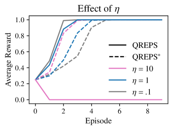
Figure 4: Effect of relative entropy regularization parameter $\eta$ on the performance of Q-REPS. On this figure, $\texttt{Q-REPS}^{*}$ (dashed line) refers to the ideal version of the algorithm that minimizes the exact LBE, whereas Q-REPS (solid line) is the sample-based implementation minimizing the empirical LBE. For large $\eta$, Q-REPS suffers from bias and only converges to the optimal policy for smaller values of $\eta$. This effect is independent of the sample size $N$ used for the updates. On the other hand, the ideal updates performed by $\texttt{Q-REPS}^{*}$ do not suffer from such bias.

We also note that this bias issue can be alleviated if one has access to a simulator of the environment that allows drawing states from the transition distribution $P(\cdot|x,a)$ for any state-action pair in the replay buffer. Indeed, in this case one can replace $X^{\prime}$ by an independently generated sample in the gradient estimator $\widehat{g}_{k,t}(\theta)$ defined in Equation (12), which allows convergence to the minimizer of the following semi-empirical version of the LBE:

$$\begin{split}\widetilde{\mathcal{G}}_{k}(\theta)=&\frac{1}{\eta}\log\left(\frac{1}{N}\sum_{n=1}^{N}e^{\eta\Delta_{\theta}(X_{k,n},A_{k,n})}\right)+(1-\gamma)\left\langle\nu_{0},V_{\theta}\right\rangle.\end{split}$$ (19)

As this definition replaces the empirical Bellman error by the true Bellman error in the exponent, it serves as an unbiased estimator of the LBE. Due to this property, one can set large values of the regularization parameter $\eta$ and converge faster toward the optimal policy. Thus, this implementation of Q-REPS is preferable when one has sampling access to the transition function.

B.2 The Effect of $\alpha$ on the Action Gap

One interesting feature of the Q-REPS optimization problem (9) is that it becomes essentially identical to the REPS problem (3) when setting $\alpha=+\infty$. To see this, let $\Psi$ and $\Phi$ be the identity maps so that the primal form of Q-REPS becomes

$$\begin{split}\text{maximize}_{\mu,d\in\mathcal{U}}&\quad\left\langle\mu,r\right\rangle-\frac{1}{\eta}D(\mu\|\mu_{0})\\ \text{s.t.}\quad&E^{\mathsf{\scriptscriptstyle T}}d=\gamma P^{\mathsf{\scriptscriptstyle T}}\mu+(1-\gamma)\nu_{0}\\ &d=\mu,\end{split}$$

which is clearly seen to be a simple reparametrization of the convex program (3). Furthermore, when $\alpha=+\infty$, the closed-form expression for $V$ in Proposition 1 is replaced with the inequality constraint $V(x)\geq Q(x,a)$ required to hold for all $x,a$ and the dual function becomes

$$\mathcal{G}^{\prime}(Q,V)=\frac{1}{\eta}\log\left(\sum_{x,a}{\mu_{0}(x,a)e^{\eta\left(r(x,a)+\gamma\sum_{x^{\prime}}P(x^{\prime}|x,a)V(x^{\prime})-Q(x,a)\right)}}\right)+(1-\gamma)\left\langle\nu_{0},V\right\rangle.$$

Since this function needs to be minimized in terms of $Q$ and $V$ and it is monotone decreasing in $Q$, its minimum is achieved when the constraints are tight and thus when $Q(x,a)=V(x)$ for all $x,a$. Thus, in this case $Q$ loses its intuitive interpretation as an action-value function, highlighting the importance of the conditional-entropy regularization in making Q-REPS practical.

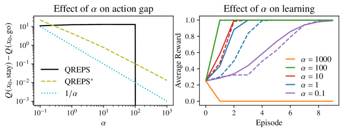
Figure 5: Effect of conditional-entropy regularization parameter $\alpha$ on the performance of Q-REPS. On this figure, $\texttt{Q-REPS}^{*}$ (dashed line) refers to the ideal version of the algorithm that minimizes the exact LBE, whereas Q-REPS (solid line) is the sample-based implementation minimizing the empirical LBE. On the left plot, we see the effect of $\alpha$ on the action gap. For $\texttt{Q-REPS}^{*}$, the action gap decreases at a rate slightly slower than $1/\alpha$. On the other hand, for Q-REPS, the estimation noise dominates the action gap for smaller values of $\alpha$. For larger values of $\alpha$, Q-REPS fails to identify the optimal action which results in a negative action gap. On the right plot, we show the performance for different values of alpha. For $\texttt{Q-REPS}^{*}$, $\alpha$ plays the role of a learning rate: as $\alpha$ increases so does the learning speed. For Q-REPS, this effect is only preserved for moderate values of $\alpha$, as the small action gap in the ideal Q-values makes identifying the optimal action harder. For $\alpha=100$ (green solid line), the sign is identified correctly and it performs almost as if no regularization was present. For $\alpha=1000$ (orange solid line), the sign is misidentified and the wrong action is preferred, leading to poor performance.

From a practical perspective, this suggests that the choice of $\alpha$ impacts the gap between the values of $Q$: as $\alpha$ goes to infinity, the gap between the values vanish and they become harder to distinguish based on noisy observations. Figure 5 shows that the action gap indeed decreases as $\alpha$ is increased, roughly at an asymptotic rate of $1/\alpha$, and that learning indeed becomes harder as the gaps decrease.

References

- Abbasi-Yadkori et al., (2019) Abbasi-Yadkori, Y., Bartlett, P., Bhatia, K., Lazic, N., Szepesvári, Cs., and Weisz, G. (2019). Politex: Regret bounds for policy iteration using expert prediction. In International Conference on Machine Learning, pages 3692–3702.
- Abdolmaleki et al., (2018) Abdolmaleki, A., Springenberg, J. T., Tassa, Y., Munos, R., Heess, N., and Riedmiller, M. (2018). Maximum a posteriori policy optimisation. In International Conference on Learning Representations.
- (3) Agarwal, A., Kakade, S., Krishnamurthy, A., and Sun, W. (2020a). FLAMBE: Structural complexity and representation learning of low rank MDPs. In Advances in Neural Information Processing Systems, pages 20095–20107.
- (4) Agarwal, A., Kakade, S. M., Lee, J. D., and Mahajan, G. (2020b). Optimality and approximation with policy gradient methods in Markov decision processes. In Conference on Learning Theory, pages 64–66.
- Antos et al., (2006) Antos, A., Szepesvári, Cs., and Munos, R. (2006). Learning near-optimal policies with Bellman-residual minimization based fitted policy iteration and a single sample path. In Conference on Learning Theory, pages 574–588.
- Ayoub et al., (2020) Ayoub, A., Jia, Z., Szepesvári, Cs., Wang, M., and Yang, L. F. (2020). Model-based reinforcement learning with value-targeted regression. In International Conference on Machine Learning, pages 463–474.
- Bagnell and Schneider, (2003) Bagnell, J. A. and Schneider, J. (2003). Covariant policy search. In International Joint Conference on Artificial Intelligence, pages 1019–1024.
- Beck and Teboulle, (2003) Beck, A. and Teboulle, M. (2003). Mirror descent and nonlinear projected subgradient methods for convex optimization. Operations Research Letters, 31(3):167–175.
- Boucheron et al., (2013) Boucheron, S., Lugosi, G., and Massart, P. (2013). Concentration inequalities: A Nonasymptotic Theory of Independence. Oxford University Press.
- Brockman et al., (2016) Brockman, G., Cheung, V., Pettersson, L., Schneider, J., Schulman, J., Tang, J., and Zaremba, W. (2016). OpenAI gym. arXiv preprint arXiv:1606.01540.
- Cai et al., (2020) Cai, Q., Yang, Z., Jin, C., and Wang, Z. (2020). Provably efficient exploration in policy optimization. In International Conference on Machine Learning.
- Cesa-Bianchi and Lugosi, (2006) Cesa-Bianchi, N. and Lugosi, G. (2006). Prediction, Learning, and Games. Cambridge University Press, New York, NY, USA.
- Curi, (2020) Curi, S. (2020). RL-Lib - a PyTorch-based library for reinforcement learning research. Github.
- Dai et al., (2018) Dai, B., Shaw, A., Li, L., Xiao, L., He, N., Liu, Z., Chen, J., and Song, L. (2018). SBEED: Convergent reinforcement learning with nonlinear function approximation. In International Conference on Machine Learning, pages 1125–1134.
- de Farias and Van Roy, (2003) de Farias, D. P. and Van Roy, B. (2003). The linear programming approach to approximate dynamic programming. Operations Research, 51(6):850–865.
- Deisenroth et al., (2013) Deisenroth, M., Neumann, G., and Peters, J. (2013). A survey on policy search for robotics. Foundations and Trends in Robotics, 2(1-2):1–142.
- Desai et al., (2012) Desai, V. V., Farias, V. F., and Moallemi, C. C. (2012). Approximate dynamic programming via a smoothed linear program. Operations Research, 60(3):655–674.
- Fan et al., (2020) Fan, J., Wang, Z., Xie, Y., and Yang, Z. (2020). A theoretical analysis of deep Q-learning. In Learning for Dynamics and Control, pages 486–489. PMLR.
- Feng et al., (2019) Feng, Y., Li, L., and Liu, Q. (2019). A kernel loss for solving the Bellman equation. In Advances in Neural Information Processing Systems, pages 15456–15467.
- Fujimoto et al., (2018) Fujimoto, S., van Hoof, H., and Meger, D. (2018). Addressing function approximation error in actor-critic methods. pages 1582–1591.
- Furmston and Barber, (2010) Furmston, T. and Barber, D. (2010). Variational methods for reinforcement learning. In Artificial Intelligence and Statistics, pages 241–248.
- Geist et al., (2017) Geist, M., Piot, B., and Pietquin, O. (2017). Is the Bellman residual a bad proxy? In Advances in Neural Information Processing Systems, pages 3205–3214.
- Geist et al., (2019) Geist, M., Scherrer, B., and Pietquin, O. (2019). A theory of regularized Markov decision processes. In International Conference on Machine Learning, pages 2160–2169.
- Haarnoja et al., (2018) Haarnoja, T., Zhou, A., Abbeel, P., and Levine, S. (2018). Soft actor-critic: Off-policy maximum entropy deep reinforcement learning with a stochastic actor. In International Conference on Machine Learning, pages 1861–1870.
- Jin et al., (2020) Jin, C., Yang, Z., Wang, Z., and Jordan, M. I. (2020). Provably efficient reinforcement learning with linear function approximation. In Conference on Learning Theory, pages 2137–2143.
- Kakade, (2001) Kakade, S. (2001). A natural policy gradient. In Advances in Neural Information Processing Systems, pages 1531–1538.
- Kakade and Langford, (2002) Kakade, S. and Langford, J. (2002). Approximately optimal approximate reinforcement learning. In International Conference on Machine Learning, volume 2, pages 267–274.
- Kingma and Ba, (2014) Kingma, D. P. and Ba, J. (2014). Adam: A method for stochastic optimization. In International Conference on Learning Representations.
- Lakshminarayanan et al., (2018) Lakshminarayanan, C., Bhatnagar, S., and Szepesvári, Cs. (2018). A linearly relaxed approximate linear program for Markov decision processes. IEEE Transactions on Automatic Control, 63(4):1185–1191.
- Lee and He, (2019) Lee, D. and He, N. (2019). Stochastic primal-dual Q-learning algorithm for discounted MDPs. In American Control Conference, pages 4897–4902.
- Manne, (1960) Manne, A. S. (1960). Linear programming and sequential decisions. Management Science, 6(3):259–267.
- Martinet, (1970) Martinet, B. (1970). Régularisation d’inéquations variationnelles par approximations successives. ESAIM: Mathematical Modelling and Numerical Analysis - Modélisation Mathématique et Analyse Numérique, 4(R3):154–158.
- Mehta and Meyn, (2009) Mehta, P. and Meyn, S. (2009). Q-learning and Pontryagin’s minimum principle. In Conference on Decision and Control, pages 3598–3605. IEEE.
- Mehta and Meyn, (2020) Mehta, P. G. and Meyn, S. P. (2020). Convex Q-learning, part 1: Deterministic optimal control. arXiv preprint arXiv:2008.03559.
- Melo and Ribeiro, (2007) Melo, F. S. and Ribeiro, M. I. (2007). Q-learning with linear function approximation. In Conference on Learning Theory, pages 308–322. Springer.
- Mnih et al., (2016) Mnih, V., Badia, A. P., Mirza, M., Graves, A., Lillicrap, T., Harley, T., Silver, D., and Kavukcuoglu, K. (2016). Asynchronous methods for deep reinforcement learning. In International Conference on Machine Learning, pages 1928–1937.
- Mnih et al., (2015) Mnih, V., Kavukcuoglu, K., Silver, D., Rusu, A. A., Veness, J., Bellemare, M. G., Graves, A., Riedmiller, M., Fidjeland, A. K., and Ostrovski, G. (2015). Human-level control through deep reinforcement learning. Nature, 518(7540):529–533.
- Neu et al., (2017) Neu, G., Jonsson, A., and Gómez, V. (2017). A unified view of entropy-regularized Markov decision processes. arXiv preprint arXiv:1705.07798.
- Neu and Pike-Burke, (2020) Neu, G. and Pike-Burke, C. (2020). A unifying view of optimism in episodic reinforcement learning. In Advances in Neural Information Processing Systems, pages 1392–1403.
- Nota and Thomas, (2020) Nota, C. and Thomas, P. S. (2020). Is the policy gradient a gradient? In Autonomous Agents and Multiagent Systems, pages 939–947.
- Paszke et al., (2017) Paszke, A., Gross, S., Chintala, S., Chanan, G., Yang, E., DeVito, Z., Lin, Z., Desmaison, A., Antiga, L., and Lerer, A. (2017). Automatic differentiation in PyTorch.
- Peters et al., (2010) Peters, J., Mülling, K., and Altun, Y. (2010). Relative entropy policy search. In AAAI Conference on Artificial Intelligence, pages 1607–1612.
- Petrik and Zilberstein, (2009) Petrik, M. and Zilberstein, S. (2009). Constraint relaxation in approximate linear programs. In International Conference on Machine Learning, pages 809–816.
- Puterman, (1994) Puterman, M. L. (1994). Markov Decision Processes: Discrete Stochastic Dynamic Programming. Wiley-Interscience.
- Riedmiller, (2005) Riedmiller, M. (2005). Neural fitted Q iteration–first experiences with a data efficient neural reinforcement learning method. In European Conference on Machine Learning, pages 317–328. Springer.
- Robbins and Monro, (1951) Robbins, H. and Monro, S. (1951). A stochastic approximation method. Annals of Mathematical Statistics, 22:400–407.
- Rockafellar, (1976) Rockafellar, R. T. (1976). Monotone Operators and the Proximal Point Algorithm. SIAM Journal on Control and Optimization, 14(5):877–898.
- Schaul et al., (2016) Schaul, T., Quan, J., Antonoglou, I., and Silver, D. (2016). Prioritized experience replay. In International Conference on Learning Representations.
- Scherrer et al., (2015) Scherrer, B., Ghavamzadeh, M., Gabillon, V., Lesner, B., and Geist, M. (2015). Approximate modified policy iteration and its application to the game of tetris. Journal of Machine Learning Research, 16:1629–1676.
- Schulman et al., (2015) Schulman, J., Levine, S., Abbeel, P., Jordan, M., and Moritz, P. (2015). Trust region policy optimization. In International Conference on Machine Learning, pages 1889–1897.
- Schulman et al., (2017) Schulman, J., Wolski, F., Dhariwal, P., Radford, A., and Klimov, O. (2017). Proximal policy optimization algorithms. arXiv preprint arXiv:1707.06347.
- Schweitzer and Seidmann, (1985) Schweitzer, P. and Seidmann, A. (1985). Generalized polynomial approximations in Markovian decision processes. J. of Math. Anal. and Appl., 110:568–582.
- Song et al., (2020) Song, H. F., Abdolmaleki, A., Springenberg, J. T., Clark, A., Soyer, H., Rae, J. W., Noury, S., Ahuja, A., Liu, S., Tirumala, D., Heess, N., Belov, D., Riedmiller, M. A., and Botvinick, M. M. (2020). V-MPO: on-policy maximum a posteriori policy optimization for discrete and continuous control.
- Strehl and Littman, (2008) Strehl, A. L. and Littman, M. L. (2008). An analysis of model-based interval estimation for Markov decision processes. Journal of Computer and System Sciences, 74(8):1309–1331.
- Sutton and Barto, (2018) Sutton, R. and Barto, A. (2018). Reinforcement Learning: An Introduction (second edition). MIT Press.
- Thomas, (2014) Thomas, P. (2014). Bias in natural actor-critic algorithms. In International Conference on Machine Learning, pages 441–448.
- (57) Vieillard, N., Kozuno, T., Scherrer, B., Pietquin, O., Munos, R., and Geist, M. (2020a). Leverage the average: an analysis of KL regularization in reinforcement learning. In Advances in Neural Information Processing Systems, pages 12163–12174.
- (58) Vieillard, N., Pietquin, O., and Geist, M. (2020b). Munchausen reinforcement learning. In Advances in Neural Information Processing Systems, pages 4235–4246.
- Wang et al., (2020) Wang, R., Du, S. S., Yang, L., and Salakhutdinov, R. R. (2020). On reward-free reinforcement learning with linear function approximation. In Advances in Neural Information Processing Systems, pages 17816–17826.
- Xie and Jiang, (2020) Xie, T. and Jiang, N. (2020). approximation schemes for batch reinforcement learning: A theoretical comparison. In Uncertainty in Artificial Intelligence, pages 550–559.
- Yang and Wang, (2019) Yang, L. F. and Wang, M. (2019). Sample-optimal parametric Q-learning using linearly additive features. In International Conference on Machine Learning, pages 12095–12114.
- Ziebart et al., (2008) Ziebart, B., Maas, A. L., Bagnell, J. A., and Dey, A. K. (2008). Maximum entropy inverse reinforcement learning. In AAAI Conference on Artificial Intelligence, pages 1433–1438.
- Zimin and Neu, (2013) Zimin, A. and Neu, G. (2013). Online learning in episodic Markovian decision processes by relative entropy policy search. In Advances in Neural Information Processing Systems, pages 1583–1591.