Finite-size localization scenarios in condensation transitions

Abstract

We consider the phenomenon of condensation of a globally conserved quantity $H=\sum_{i=1}^{N}\epsilon_{i}$ distributed on $N$ sites, occurring when the density $h=H/N$ exceeds a critical density $h_{c}$. We numerically study the dependence of the participation ratio $Y_{2}=\langle\epsilon_{i}^{2}\rangle/(Nh^{2})$ on the size $N$ of the system and on the control parameter $\delta=(h-h_{c})$, for various models: (i) a model with two conservation laws, derived from the Discrete NonLinear Schrödinger equation; (ii) the continuous version of the Zero Range Process class, for different forms of the function $f(\epsilon)$ defining the factorized steady state. Our results show that various localization scenarios may appear for finite $N$ and close to the transition point. These scenarios are characterized by the presence or the absence of a minimum of $Y_{2}$ when plotted against $N$ and by an exponent $\gamma\geq 2$ defined through the relation $N^{*}\simeq\delta^{-\gamma}$, where $N^{*}$ separates the delocalized region ($N\ll N^{*}$, $Y_{2}$ vanishes with increasing $N$) from the localized region ($N\gg N^{*}$, $Y_{2}$ is approximately constant). We finally compare our results with the structure of the condensate obtained through the single-site marginal distribution.

I Introduction

The word condensation typically refers to the condensation of a gas Chaikin et al. (1995), a classical change of the physical state of matter, or to the Bose-Einstein condensation (BEC), a quantum phenomenon observed in dilute atomic gases Huang (1987). In the last twenty years it has acquired a new meaning related to transport phenomena: under certain conditions it may appear a critical density of the transported quantity (e.g., mass) above which a finite fraction of whole mass condenses/localizes at a single site of a lattice Drouffe et al. (1998); Majumdar et al. (2005); Godreche (2007); Majumdar (2010); Zannetti et al. (2014); Godrèche (2020). It is therefore a localization in the real space while BEC is a localization in the momentum space.

The phenomenon of real-space condensation appears ubiquitously in several domains of physics, ranging from shaken granular materials Eggers (1999); Török (2005) to the behavior of traffic flows Evans and Hanney (2005), just to mention a couple of important applications. Another physically relevant example appears when studying the Discrete NonLinear Schrödinger (DNLS) equation Kevrekidis (2009), which is used to model nonlinear wave propagation in weakly dissipative systems with important applications in the fields of nonlinear optics Eisenberg et al. (1998) and cold atoms Trombettoni and Smerzi (2001). In this context, in spite of the presence of two conservation laws (see Sec. II), it has recently been shown Gradenigo et al. (2021a, b) that the condensation transition of the DNLS model is strictly related to a special case of the class of zero-range processes (ZRP) Evans and Hanney (2005), where only one quantity is conserved. In the wide class of ZRP, the sites of a lattice hosts indistinguishable particles which hop from a site $i$ to a neighboring site $i^{\prime}$ with a rate depending only on the number of particles at the departure site $i$. The peculiarity of ZRP class and of its continuous version Evans et al. (2004); Zia et al. (2004) is that stationary/equilibrium states are given by a simple factorized form Evans and Hanney (2005), which may allow for analytic descriptions of the condensation process Evans et al. (2006).

Finite-size effects play a relevant role in condensation transitions, as they can determine the dominant behavior of the system even for moderately large system sizes. As an example, in the DNLS model they are responsible of the emergence of peculiar delocalized states at negative absolute temperature. Such states disappear in the thermodynamic limit, but they are still easily detectable even for lattices of thousands of sites Gradenigo et al. (2021a, b).

In this paper we provide a systematic numerical study of the localization process occurring at finite sizes and for different classes of condensation models. In order to be specific, let us suppose to have $N$ independent random variables $\epsilon_{i}$, equally distributed according to some distribution function $f(\epsilon)$ and constrained by their sum, $\sum_{i}\epsilon_{i}=H\equiv Nh$ Godrèche and Luck (2001). Condensation is known to occur if asymptotically ($\epsilon\to\infty$) Evans et al. (2006)

$$\exp(-\epsilon)<f(\epsilon)<\frac{1}{\epsilon^{2}},$$ (1)

and if $h>h_{c}$, with the critical value for condensation given by

$$h_{c}=\int_{0}^{\infty}\!\!d\epsilon\,\epsilon f(\epsilon)\;.$$ (2)

In the condensed region, $h\geq h_{c}$, and in the thermodynamic limit $N\to\infty$, the equilibrium state is trivial: one single site $i^{*}$ collects the “extra” energy above the threshold, $\epsilon_{i^{*}}=\delta N\equiv(h-h_{c})N$, while the “critical” energy $h_{c}N$ is distributed to all other sites according to $f(\epsilon)$.

When the system is finite, the above picture must be corrected evaluating the single-site marginal distribution,

$$p(\epsilon)=f(\epsilon)\frac{Z_{N-1}(E-\epsilon)}{Z_{N}(E)},$$ (3)

where $Z_{N}(E)=\int d\epsilon_{1}\dots d\epsilon_{N}\prod_{k=1}^{N}f(\epsilon_{k})\delta(E-\sum_{i}\epsilon_{i})$ is the partition function. This has been done in Ref. Evans et al. (2006) where it is derived the limiting shape of the condensate, i.e. the form of the distribution (3) around $\epsilon=\delta N$.

Here we focus on the finite-size effects of the condensation transition close to the critical point ($\delta\ll 1,N\gg 1$) using the participation ratio,

$$Y_{2}(N,\delta)\equiv\frac{\langle\,\overline{\epsilon_{i}^{2}}\,\rangle}{\displaystyle N\langle\,\overline{\epsilon_{i}}\,\rangle^{2}}=\frac{\langle\,\overline{\epsilon_{i}^{2}}\,\rangle}{Nh^{2}}\,,$$ (4)

where $\overline{(\cdots)}$ is a spatial average and $\langle\cdots\rangle$ is a statistical average. $Y_{2}$, firstly introduced in the theory of electron localization Thouless (1974), has been recently used in the context of condensation transitions Gradenigo and Bertin (2017); Gradenigo et al. (2021a, b). Most importantly, it should be noted that $Y_{2}$ is a collective property which represents the proper order parameter for the condensation/localization transition, as it allows to discriminate between homogeneous and localized states. In the former case $\langle\,\overline{\epsilon_{i}}\,\rangle^{2}$ is finite and $Y_{2}$ asymptotically vanishes as $1/N$. In the latter case the average is dominated by the single site hosting the extra-energy, $\langle\,\overline{\epsilon_{i}^{2}}\,\rangle=N\delta^{2}+o(N)$ and in the thermodynamic limit $Y_{2}$ remains finite:

$$Y_{2}^{\infty}(\delta)=\frac{\delta^{2}}{h^{2}}=\frac{\delta^{2}}{(h_{c}+\delta)^{2}}\,.$$ (5)

For finite system sizes it is no more possible to assume that a single site hosts all the excess energy as soon as $\delta>0$ and the evaluation of $Y_{2}$ is much more complicated. The full knowledge of $p(\epsilon)$, see Eq. (3), would allow to compute $Y_{2}(N,\delta)$ but in practice this is hardly feasible in general. For this reason in the following we will carry out a detailed numerical analysis of how $Y_{2}(N,\delta)$ depends on the size $N$ and on the reduced control parameter $\delta=h-h_{c}$, for several models. In particular, the use of the participation ratio will allow to characterize the condensation transition through some qualitative and quantitative features which will be seen to depend on the asymptotic form of $f(\epsilon)$. A detailed description of the content of the paper follows.

We start in Sec. II with the DNLS equation, showing the well known result that close to the transition point it reduces to a simple microcanonical model with two conservation laws, called here C2C model. Our analysis shows that $Y_{2}(N,\delta)$ does not tend to the asymptotic value $Y_{2}^{\infty}(\delta)$ monotonically: it displays a minimum as a function of $N$ and $Y_{2}^{min}(\delta)\sim\delta^{\gamma}$ with $\gamma=3$. The study of the participation ratio therefore allows to introduce the exponent $\gamma$.

In Sec. III we pass to study different cases of the “continuous mass” transport models, i.e. different functions $f(\epsilon)$ in the condensation range defined in Eq. (1). Since the transported quantity is continuous and we focus on the equilibrium properties we will use the acronym FCT (Factorized Continuous Transport) to indicate these models. We will start by discussing a recent result Gradenigo et al. (2021a) according to which the C2C model is asymptotically equivalent to the FCT model where $f(\epsilon)$ is a stretched-exponential distribution, $f(\epsilon)\sim\exp(-\sqrt{\epsilon})$. The following analysis of the participation ratio for the cases where $f(\epsilon)$ decays as a power law $1/\epsilon^{\beta}$ shows localization scenarios which are different from the C2C one: when $\beta=4$, $Y_{2}$ still displays a minimum as a function of $N$ but with a different exponent $\gamma=2$, because now $Y_{2}^{min}(\delta)\sim\delta^{2}$. Moreover, when $\beta=2.5$ there is no minimum at all. All the scenarios emerging from numerics will be interpreted in terms of the effective number of sites hosting the condensate, $K(N,\delta)$.

Finally, in Sec. IV we summarize our results and discuss the different localization scenarios in the light of related studies on ZRP/FCT models Evans et al. (2006) and on the C2C model Gradenigo et al. (2021a).

II The microcanonical DNLS/C2C model

The one-dimensional Discrete NonLinear Schrödinger (DNLS) model is defined by the Hamiltonian Kevrekidis (2009)

$${H}=\sum_{n}\left(|z_{n}|^{4}+z_{n}^{*}z_{n+1}+z_{n}z_{n+1}^{*}\right),$$ (6)

where $z_{n}=\rho_{n}e^{i\phi_{n}}$ are complex variables whose canonically-conjugated variables are $-iz^{*}_{n}$. Accordingly, the DNLS equation is derived from the Hamilton’s equations $\dot{z}_{n}=\partial{H}/\partial(-iz^{*}_{n})$ and reads,

$$i\dot{z}_{n}=-2|z_{n}|^{2}z_{n}-z_{n+1}-z_{n-1}\,.$$ (7)

This model has two conserved quantities, the energy (because ot time invariance of ${H}$) and the mass $A=\sum_{n}|z_{n}|^{2}$ (because of the invariance under global phase transformations, $z_{n}\to z_{n}e^{i\bar{\phi}}$). Two results are now well established Rasmussen et al. (2000); Iubini et al. (2013, 2014); Szavits-Nossan et al. (2014); Iubini et al. (2017); Gradenigo et al. (2021a): (i) this model has an equilibrium localized state for $h>h_{c}=2a^{2}$, where $a=A/N$ is the mass density, ${h}={H}/N$ is the energy density, and the curve $h_{c}=2a^{2}$ also corresponds to the infinite-temperature line. (ii) Close to this line the coupling terms between neighboring sites (see Eq. (6)), $z_{n}^{*}z_{n+1}+z_{n}z_{n+1}^{*}$, are negligible Gradenigo et al. (2021a), so that the phases $\phi_{n}$ can be ignored. In this limit the DNLS model is equivalent to a much simpler system, which is defined in terms of the positive-definite local masses $c_{i}=\rho_{i}^{2}$ and their squares (local energies) $\epsilon_{i}=c_{i}^{2}$. The total mass and energy

$$A=\sum_{i=1}^{N}c_{i},\qquad H=\sum_{i=1}^{N}\epsilon_{i}.$$ (8)

are conserved and it can be shown Gradenigo et al. (2021a) that the condensation condition $h>h_{c}=2a^{2}$ still holds, with the same meaning of the symbols $a$ and $h$ defined above. We refer to this model as the C2C model. In this model the density $a$ is just a unit of measure of the mass and we can set $a=1$ without loss of generality.

The existence of a condensation transition can be understood in the C2C model as follows. The ground state corresponds to a perfectly homogeneous state with all sites hosting the same mass, $c_{i}\equiv 1$, so $h_{GS}=1$. Upon increasing the energy ($h>1$), mass fluctuations increase evenly until $h=2$, where $\langle c_{i}^{2}\rangle=2\langle c_{i}\rangle^{2}$. Therefore at $h=2$ the standard deviation of the mass distribution is equal to its average value and the injection of additional energy is expected to be localized. According to Rasmussen et al. (2000) at criticality ($h=2$) the mass is distributed exponentially

$$\tilde{f}(c)=\exp(-c).$$ (9)

Above criticality (and in the thermodynamic limit!) a single site hosts the extra energy $\delta N$.

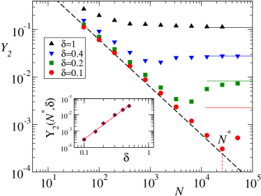
Figure 1: Curves of $Y_{2}(N,\delta)$ of the C2C model for some values of $\delta$, see legend. The black dashed curve shows the analytical scaling $Y_{2}=6/N$, expected for $N\ll N^{*}$. Full lines are the analytical asymptotic values, equal to $\delta^{2}/h^{2}$. Inset: behavior of the minimum $Y_{2}(N^{*},\delta)$ as a function of $\delta$ (black diamonds). The red line shows a growth as $\delta^{3}$.

The equilibrium properties of the C2C model, in particular the evaluation of the participation ratio $Y_{2}(N,\delta)$, see Eq. (4), have been obtained here numerically through a Microcanonical Monte Carlo algorithm. The simplest stochastic evolution rule satisfying detailed balance and conservation laws is Iubini et al. (2014) to choose a triplet of distinct sites $(i,j,k)$ and update their masses in order to conserve their sum (the mass) and the sum of their squares (the energy). This procedure amounts to determine the intersection between the plane $c_{i}+c_{j}+c_{k}=M$ with the sphere $c_{i}^{2}+c_{j}^{2}+c_{k}^{2}=E$ and to choose a random point in such intersection. If the masses are of the same order the intersection is a circle, otherwise the positivity constraint on the masses limits the intersection to the union of three arcs. The three sites can be chosen either in sequence, ($i-1,i,i+1$), or randomly. This choice affects the relaxation dynamics towards the equilibrium condensed state, which displays a coarsening process and has been studied in detail Iubini et al. (2014, 2017) for a triplet of neighboring sites. Here, instead, we will focus on the properties of the equilibrium state, which are not affected by such a choice. Accordingly, we implement the update of random triplets of sites in order to speed up numerical simulations . Finally, we stress that the energy $h$ does not enter explicitly the evolution rule: $h$ only specifies the initial configuration, which is appropriately chosen so as to have $\bar{\epsilon}_{i}=h$.

In Fig. 1 we plot $Y_{2}$ versus $N$ for different values of $\delta$. The main feature of these curves is that $Y_{2}$ does not tend to the asymptotic value $Y_{2}^{\infty}(\delta)=\delta^{2}/h^{2}$ monotonically: except for large values of $\delta$, the participation ratio has a minimum, occurring for $N=N^{*}(\delta)$ and separating the delocalized regime (where $Y_{2}$ decays as $1/N$ and does not depend on $\delta$) from a localized one, where $Y_{2}\to Y_{2}^{\infty}(\delta)$. Furthermore, according to the inset the participation ratio at the minimum vanishes with $\delta$ as a power law, $Y_{2}(N^{*},\delta)\simeq\delta^{\gamma}$, which allows to define the exponent $\gamma=3$.

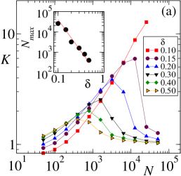
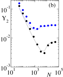
Figure 2: (a) Effective number of localization sites for the C2C model, $K(N,\delta)$, for different values of $\delta$. Inset: Size $N_{max}$ for which the maximum of $K(N)$ is attained versus $\delta$. The red curve is a power-law scaling as $\delta^{-3}$. (b)  Participation ratio directly obtained from numerics (full circles) and reproduced from Eq. (10) using data for $K$ as given in (a) (dotted lines). Data refer to $\delta=0.4$ (blue symbols, upper curve) and $\delta=0.2$ (black symbols, lower curve).

In the absence of an exact analytic expression for $Y_{2}(N,\delta)$ we propose a phenomenological interpretation of our results which is also applicable to the models studied in the next Section. The basic assumption is that the extra energy $\delta N$ is equally shared among $K(N,\delta)$ sites, while the remaining energy is homogeneously distributed on the other sites with a second moment equal to $\mu_{2}$. With these hypotheses from Eq. (4) we obtain

$$Y_{2}(N,\delta)=\frac{\mu_{2}}{Nh^{2}}+\frac{\delta^{2}}{K(N,\delta)h^{2}}+o\left(\frac{1}{N}\right)\,,$$ (10)

which immediately clarifies that the condition $K=1$ (or $K$ any constant) cannot produce a minimum in $Y_{2}$. More precisely, if we take the derivative of $Y_{2}$ with respect to $N$ we obtain

$$\frac{dY_{2}}{dN}=-\frac{\mu_{2}}{N^{2}h^{2}}-\frac{\delta^{2}}{K^{2}h^{2}}\frac{dK}{dN},$$ (11)

indicating that a minimum of $Y_{2}(N,\delta)$ ($dY_{2}/dN=0$) may appear only if $K(N,\delta)$ decreases in some interval of $N$ ($dK/dN<0$).

The correctness of this interpretation is shown in Fig. 2. In left panel (a) the effective number of sites hosting the extra energy, $K(N,\delta)$, has been independently derived from simulations comparing the extra energy with the actual, maximal energy appearing in the lattice: their ratio gives an estimate of $K(N,\delta)$. The curves $K(N,\delta)$ have a maximum which can explain the minimum of the participation ratio. Furthermore, the position of the maximum $N_{max}$ moves to larger $N$ when $\delta$ decreases (which is in agreement with a decreasing function $N^{*}(\delta)$) and the maximum itself increases upon decreasing $\delta$ (which is in agreement with the fact that $Y_{2}(N^{*})$ decreases more rapidly than $Y_{2}^{\infty}$). The inset of Fig. 2(a) shows that $N_{max}(\delta)$ scales as $\delta^{-3}$, that is, as $N^{*}(\delta)$. If we now make use of the just determined function $K(N,\delta)$ in Eq. (10), we obtain the curves $Y_{2}(N,\delta)$ as given in Fig. 2(b) (see dotted lines), which satisfactorily reproduce the behavior of the participation ratio in the whole range of $N$, attesting the correctness of the proposed expression (10) for $Y_{2}(N,\delta)$.

The next step is to understand whether the features of $Y_{2}(N,\delta)$ we have found for the C2C model (existence of a minimum and value of the exponent $\gamma$) are either model-specific or generic. For this reason we now move to study the more general class of FCT models. This passage is even more justified by the strict connection between C2C and FCT, as now discussed.

III Canonical FCT models

In Ref. Gradenigo et al. (2021a) the microcanonical partiton function of the C2C model,

$$\Omega(A,E)=\int_{0}^{\infty}\!\!\prod_{i}dc_{i}\,\,\delta\!\left(A-\sum_{i}c_{i}\right)\delta\!\left(E-\sum_{i}c_{i}^{2}\right),$$ (12)

was studied by means of large-deviations techniques. It was shown that the constraint on the mass conservation can be relaxed by taking the Laplace transform with respect to $A$, explicitly

$$\tilde{\Omega}(\lambda,E)=\left(\frac{1}{2\lambda}\right)\int_{0}^{\infty}\!\!\prod_{i}d\epsilon_{i}f_{\lambda}(\epsilon_{i})\delta\!\left(E-\sum_{i}\epsilon_{i}\right)$$ (13)

where 

$$f_{\lambda}(\epsilon)=\frac{\lambda}{2\sqrt{\epsilon}}\exp(-\lambda\sqrt{\epsilon}).$$ (14)

Equation (13) can be therefore interpreted as the probability distribution of the sum of $N$ i.i.d. random variables $\epsilon_{i}$ distributed according to $f_{\lambda}(\epsilon)$ and constrained by the their sum. Since $f_{\lambda}(\epsilon)$ satisfies the bounds of Eq. (1) this is a further proof that the C2C model has a condensation transition. The equivalence between the microcanonical C2C model and the canonical FCT model with a distribution given by Eq. (14) is only guaranteed in the thermodynamical limit. For this reason we have explicitly simulated the canonical FCT model with a pure stretched exponential,

$$f_{s}(\epsilon)=\frac{3}{2}\exp(-\sqrt{3\epsilon}),$$ (15)

where the $\sqrt{3}$ factor at the exponent has been chosen so as to have $h_{c}=\int_{0}^{\infty}\!\!d\epsilon\,\epsilon f_{s}(\epsilon)=2$.

Simulations have been performed using the following Monte Carlo algorithm to sample the equilibrium state Godrèche and Luck (2001). Two distinct sites $i,j$ are randomly chosen and a random energy value $\epsilon^{*}$ is extracted from a uniform distribution in the interval $(0,\epsilon_{i}+\epsilon_{j})$. The attempted new energies are $\epsilon^{\prime}_{i}=\epsilon^{*}$ and $\epsilon^{\prime}_{j}=(\epsilon_{i}+\epsilon_{j})-\epsilon^{*}$. This move, which by construction conserves the energy, is accepted with probability

$$q = \min\{1,q^{*}\},$$

$$q^{*} = \frac{f_{\beta}(\epsilon^{\prime}_{i})f_{\beta}(\epsilon^{\prime}_{j})}{f_{\beta}(\epsilon_{i})f_{\beta}(\epsilon_{j})},$$ (16)

which satisfies detailed balance. Results are shown in Fig. 3: not only a clear minimum of the participation ratio appears, it also scales with an exponent compatible with $\gamma=3$.

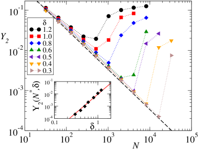
Figure 3: Curves of $Y_{2}(N,\delta)$ for $f_{s}(\epsilon)=\frac{3}{2}\exp(-\sqrt{3\epsilon})$. The black dashed curve shows the analytical scaling $Y_{2}=10/(3N)$, expected for $N\ll N^{*}$. Inset: behavior of the minimum $Y_{2}(N^{*},\delta)$ as a function of $\delta$ (black diamonds). The red line shows a growth as $\delta^{3}$.

In order to check how peculiar are the properties of the C2C model and of the FCT model with $f(\epsilon)=f_{s}(\epsilon)$, it is now necessary to study definitely different $f(\epsilon)$. For this reason we will focus to the family of power-law distributions

$$f_{\beta}(\epsilon)=\frac{1}{b_{0}+\epsilon^{\beta}},$$ (17)

where the real parameter $\beta$ satisfies the condition $\beta>2$ in order to have a condensation phenomenon, see Eq. (1), and $b_{0}$ is fixed to have the same critical value as the C2C model,

$$h_{c}=\frac{\int_{0}^{\infty}d\epsilon\epsilon f_{\beta}(\epsilon)}{\int_{0}^{\infty}d\epsilon f_{\beta}(\epsilon)}=2.$$ (18)

Expression (10) for the participation ratio suggests that a distinction should be made between $\beta>3$ and $\beta\leq 3$. In the former case $f_{\beta}(\epsilon)$ has a finite second moment, while in the latter case $\mu_{2}$ diverges as $N^{3-\beta}$ (logarithmically for $\beta=3$) . All the same, the first term on the RHS of Eq. (10) vanishes asymptotically for $\beta>2$. Therefore in such limit it is negligible with respect to the second term which tends to $\delta^{2}/h^{2}$.

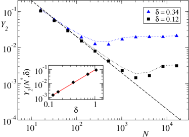
Figure 4: Participation ratio of the $\beta=4$ model for a couple of values of $\delta$ (full symbols). Dotted lines refer to the values obtained from Eq. (10). The straight dashed line is the analytical expression $Y_{2}(N,\delta=0)=2/N$, valid for $N\ll N^{*}$. Inset: $Y_{2}(N^{*},\delta)$ as a function of $\delta$ (black diamonds). The red line shows a growth as $\delta^{2}$.

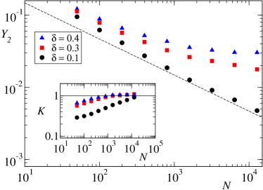
Figure 5: Participation ratio of the $\beta=2.5$ model for different values of $\delta$. $Y_{2}(N,\delta)$ curves at $\delta$ fixed have no minimum, in agreement with the absence of a maximum in the curves $K(N)$, see the inset. Furthermore, for $N\ll N^{*}$ $Y_{2}(N)$ decays as $1/N^{1/2}$, see dashed line.

We have studied this class of models for $\beta=4$ and $\beta=2.5$ Results are shown in Fig. 4 for $\beta=4$ and in Fig. 5 for $\beta=2.5$. For $\beta=4$, $Y_{2}$ displays a minimum similarly to the C2C model, but, as shown in the inset, there is an important difference between the two models because $\gamma$(C2C)$=3$, while $\gamma(\beta=4)=2$. Accordingly, for finite systems, delocalized states extend above the critical threshold up to sizes of order $N^{*}$, with

$$N^{*}(\beta=4)\sim\delta^{-2}\ll N^{*}(C2C)\sim\delta^{-3}.$$ (19)

From the derivation of the curves $K(N,\delta)$ as explained for the C2C model and from Eq. (10), again, we are able to reproduce the $N-$dependence of the participation ratio for different values of $\delta$, see Fig. 4 (main).

When the exponent $\beta$ is reduced, the minimum of $Y_{2}$ can even disappear, as observed for $\beta=2.5$, see Fig. 5. The monotonic decrease of $Y_{2}$ towards the finite asymptotic value is compatible with a localization transition involving condensation on a single site also for finite $N$. In fact, for $\beta=2.5$ no peak exists in $K$ versus $N$, see the inset. The absence of a decreasing regime for $K$ implies the absence of a minimum for $Y_{2}$. Furthermore, we observe that the first term on the RHS of Eq. (10) does not decrease as $1/N$ because the second moment $\mu_{2}$ at the numerator diverges for $\beta<3$. More precisely, such term vanishes as $1/N^{\beta-2}$, which explains the decay $Y_{2}\sim 1/\sqrt{N}$ observed in Fig. 5. In the absence of a minimum, $N^{*}$ can be interpreted as a size separating the delocalized phase from the localized one and it can be derived by equating the two terms of Eq. (10). For $\beta=2.5$ we have $1/\sqrt{N^{*}}\sim\delta^{2}$, therefore $N^{*}(\beta=2.5)=\delta^{-4}$. Using the relation $N^{*}(\beta)\simeq\delta^{-\gamma}$ we can define the exponent $\gamma$ also if $Y_{2}$ does not display a minimum and obtain $\gamma(\beta=2.5)=4$.

IV Discussion

In the thermodynamic limit the main properties of the localization transition are well understood: (i) Eq. (1) gives the condensation condition for the class of the discrete Zero Range Process (ZRP) models and for their continuous counterpart, that we called here Factorized Continuous Transport (FCT) models. (ii) At criticality the single-site marginal distribution function $p(\epsilon)$ in Eq. (3) equals the function $f(\epsilon)$. Above criticality $p(\epsilon)$ is given by $f(\epsilon)$ plus a Dirac delta centred at the energy excess $N\delta$; (iii) The value of the participation ratio in the thermodynamic limit is simply $Y_{2}^{\infty}(\delta)=(\delta/h)^{2}$.

When the finite size $N$ is taken into account things get more complicated but also more interesting, as physically relevant phenomena may appear. In this paper, we studied numerically several condensation models focusing on the behavior of the participation ratio $Y_{2}(N,\delta)$, which is the standard order parameter Godrèche and Luck (2012); Gradenigo and Bertin (2017); Gradenigo et al. (2021a) as well as an experimentally accessible observable, see e.g. Lahini et al. (2009).

Concerning the C2C model, our results are in agreement with the recent analytical results obtained in Ref. Gradenigo et al. (2021a) using the large deviation theory. Our study confirms that for finite $N$ the system is still nonlocalized for $\delta<\delta^{*}\sim 1/N^{1/3}$ and it shows that the transition between the nonlocalized and localized regimes corresponds to a minimum of the participation ratio. The large extension of the nonlocalized region is related to an exponent $\gamma=3$. In the context of the DNLS equation where localized states are generated dynamically as discrete breather excitations Flach and Willis (1998); Flach and Gorbach (2008), these results corroborate the idea that multi-breather states are compatible with equilibrium conditions, as discussed in Iubini et al. (2013). We have also shown that, consistently with Gradenigo et al. (2021a), analogous results hold for a canonical FCT model characterized by a stretched-exponential distribution.

The above properties are modified for FCT models with power-law distributions, $f(\epsilon)\sim 1/\epsilon^{\beta}$ $(\beta>2)$. More precisely, we have studied two cases, $\beta=4$ and $\beta=2.5$. For $\beta=4$, $Y_{2}$ still displays a minimum in $N$, yet $\gamma=2$. This means that $\gamma$ has the lowest possible value, so that, for finite $N$ and $\delta>0$, the delocalized region has the smallest possible extension in $N$. For $\beta=2.5$, $Y_{2}$ does not even have a minimum. Moreover, since the second moment of the distribution diverges, the nonlocalized region is “strongly” nonlocalized, because $Y_{2}$ decays as $1/\sqrt{N}$ rather than as $1/N$. Even if a minimum does not exist, it is possible to define $N^{*}$ as the length separating the nonlocalized region $(N\ll N^{*})$ from the localized one $(N\gg N^{*})$ and it is therefore possible to define the exponent $\gamma$ through the relation $N^{*}\simeq\delta^{-\gamma}$. With this definition, we can sum up our findings: $\gamma(\beta=2.5)=4$, $\gamma(\beta=4)=2$, $\gamma(\mbox{stretched-exponential})=\gamma(\mbox{C2C})=3$.

We also stress that significantly different localization scenarios can have a unified interpretation through the effective number of sites hosting the condensate, $K(N,\delta)$, which determines the participation ratio, see Eq. (10). In fact, the minimum of $Y_{2}(N)$ is related to a maximum of $K(N)$ and the exponent $\gamma>2$ is related to a maximum of $K(N)$ whose value increases upon decreasing $\delta$. The non-monotonic behavior of $Y_{2}(N)$ has also important physical implications for what concerns the observation of effectively delocalized states above the critical condensation point, as recently discussed in Gradenigo et al. (2021a) for the DNLS model.

It is useful to compare our results with related studies of the nature of the condensate based on the single-site marginal distribution Evans et al. (2006). The case $\beta=4$ corresponds to gaussian fluctuations of the condensate (called normal condensate) on the scale $|\epsilon-\delta N|\sim N^{2/3}$ while the case $\beta=2.5$ corresponds to non gaussian fluctuations of the condensate (called anomalous condensate). Finally, the stretched-exponential case is characterized by gaussian fluctuations but on the different scale $|\epsilon-\delta N|\sim N^{1/2}$. Additionally, in Evans et al. (2006) it was also noted that the nature of the condensation transition for stretched exponential distributions differs from the usual scenario of a second order phase transition. In fact, specific signatures of a first order phase transition have been recently found in Gradenigo and Majumdar (2019); Gradenigo et al. (2021a). In Fig. 6 we show a schematic phase diagram which summarizes our results and the results obtained in Evans et al. (2006). We also mention that we have obtained preliminary results for the model $\beta=6$ and for a modified stretched-exponential distribution, $f(\epsilon)\sim\exp(-\epsilon^{0.6})$. Results clearly show that in both cases $Y_{2}$ has a minimum in $N$ and suggest that $\gamma=2$ for $\beta=6$ and $\gamma=3$ for the modified stretched-exponential case.

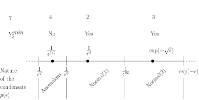
Figure 6: Localization properties for canonical FCT models with distributions in the range $1/\epsilon^{2}>f(\epsilon)>\exp(-\epsilon)$. Upper half: behavior of $Y_{2}^{min}$ and $\gamma$ obtained in the present article for the specific models indicated by the full dots (the results for the stretched exponential case are also representative of the C2C model). Lower half: nature of the condensate as obtained in Evans et al. (2006) through the single-site marginal distribution $p(\epsilon)$. Normal (Anomalous) means that fluctuations of the condensate are (are not) gaussian. Normal$(1)$ and Normal$(2)$ refer to different scales over which fluctuations are gaussian (see the main text).

In order to clarify the full localization scenarios in the whole range of distributions given in Eq. (1) it will be necessary to perform detailed simulations for several other models, keeping in mind that larger values of $\gamma$ would be very problematic for numerics, because $N^{*}$ scales as $1/\delta^{\gamma}$, therefore forcing to investigate extremely large systems. Alternatively, analytic approaches allowing to extract the peculiar features that make a model fall in a given scenario would be desirable. We hope that our results might lead to pursue further analytical studies to find a rigorous connection between the properties of $Y_{2}$ and $K$ on the one hand and those of $p(\epsilon)$ on the other hand.