MADER: Trajectory Planner in Multi-Agent and Dynamic Environments

Abstract

This paper presents MADER, a 3D decentralized and asynchronous trajectory planner for UAVs that generates collision-free trajectories in environments with static obstacles, dynamic obstacles, and other planning agents. Real-time collision avoidance with other dynamic obstacles or agents is done by performing outer polyhedral representations of every interval of the trajectories and then including the plane that separates each pair of polyhedra as a decision variable in the optimization problem. MADER uses our recently developed MINVO basis ([1]) to obtain outer polyhedral representations with volumes 2.36 and 254.9 times, respectively, smaller than the Bernstein or B-Spline bases used extensively in the planning literature. Our decentralized and asynchronous algorithm guarantees safety with respect to other agents by including their committed trajectories as constraints in the optimization and then executing a collision check-recheck scheme. Finally, extensive simulations in challenging cluttered environments show up to a 33.9% reduction in the flight time, and a 88.8% reduction in the number of stops compared to the Bernstein and B-Spline bases, shorter flight distances than centralized approaches, and shorter total times on average than synchronous decentralized approaches.

Acronyms: UAV (Unmanned Aerial Vehicle), MINVO (Basis that obtains a minimum-volume simplex enclosing a polynomial curve [1]), MADER (Trajectory Planner in Multi-Agent and Dynamic Environments), AABB (Axis-Aligned Bounding Box).

Supplementary material

Video: https://youtu.be/aoSoiZDfxGE
Code: https://github.com/mit-acl/mader

I Introduction and related work

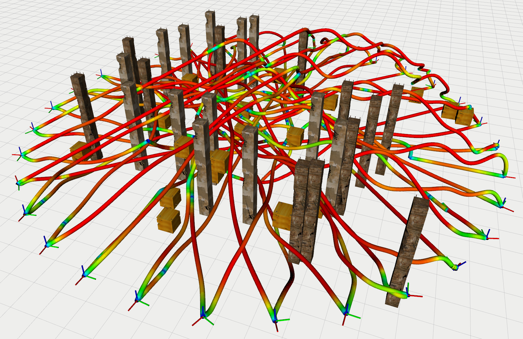
(a) Circle configuration: 32 agents, 25 static obstacles and 25 dynamic obstacles.

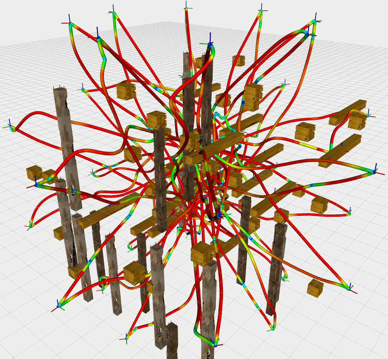
(b) Sphere configuration: 32 agents, 18 static obstacles and 52 dynamic obstacles.

Figure 1: 32 agents using MADER to plan trajectories in a decentralized and asynchronous way in an environment with dynamic obstacles (light brown boxes and horizontal poles), static obstacles (dark brown pillars) and other agents.

While efficient and fast UAV trajectory planners for static worlds have been extensively proposed in the literature [2, 3, 4, 5, 6, 7, 8, 9, 10, 11, 12, 13, 14], a 3D real-time planner able to handle environments with static obstacles, dynamic obstacles and other planning agents still remains an open problem (see Fig. 1).

To be able to guarantee safety, the trajectory of the planning agent and the ones of other obstacles/agents need to be encoded in the optimization (see Fig. 2). A common representation of this trajectory in the optimization is via points discretized along the trajectory [15, 16, 17, 18, 19, 20]. However, this does not usually guarantee safety between two consecutive discretization points and alleviating that problem by using a fine discretization of the trajectory can lead to a very high computational burden. To reduce this computational burden, polyhedral outer representations of each interval of the trajectory are extensively used in the literature, with the added benefit of ensuring safety at all times (i.e., not just at the discretization points). A common way to obtain this polyhedral outer representation is via the convex hull of the control points of the Bernstein basis (basis used by Bézier curves) or the B-Spline basis [13, 10, 21, 22]. However, these bases do not yield very tight (i.e., with minimum volume) tetrahedra that enclose the curve, leading to conservative results.

MADER addresses this conservatism at its source and leverages our recently developed MINVO basis [1] to obtain control points that generate the $n$-simplex (a tetrahedron for $n=3$) with the minimum volume that completely contains each interval of the curve. Global optimality (in terms of minimum volume) of this tetrahedron obtained by the MINVO basis is guaranteed both in position and velocity space.

When other agents are present, the deconfliction problem between the trajectories also needs to be solved. Most of the state-of-the-art approaches either rely on centralized algorithms [23, 24, 25] and/or on imposing an ad-hoc priority such that an agent only avoids other agents with higher priority [26, 27, 28, 29, 30]. Some decentralized solutions have also been proposed [31, 28, 32], but they require synchronization between the replans of different agents. The challenge then is how to create a decentralized and asynchronous planner that solves the deconfliction problem and guarantees safety and feasibility for all the agents.

MADER solves this deconfliction in a decentralized and asynchronous way by including the trajectories other agents have committed to as constraints in the optimization. After the optimization, a collision check-recheck scheme ensures that the trajectory found is still feasible with respect to the trajectories other agents have committed to while the optimization was happening.

To impose collision-free constraints in the presence of static obstacles, a common approach is to first find convex decompositions of free space and then force (in the optimization problem) the outer polyhedral representation of each interval to be inside these convex decompositions [10, 33, 34]. However, this approach can be conservative, especially in cluttered environments in which the convex decomposition algorithm may not find a tight representation of the free space. In the presence of dynamic obstacles, these convex decompositions become harder, and likely intractable, due to the extra time dimension.

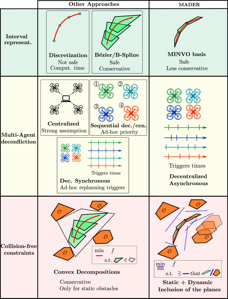
Figure 2: Contributions of MADER.

To be able to impose collision-free constraints with respect to dynamic obstacles/agents, MADER imposes the separation between the polyhedral representations of each trajectory via planes. Moreover, MADER overcomes the conservatism of a convex decomposition (imposed ad-hoc before the optimization) by including a parameterization of these separating planes as decision variables in the optimization problem. The solver can thus choose the optimal location of these planes to determine collision avoidance. Including this plane parameterization reduces conservatism, but it comes at the expense of creating a nonconvex problem, for which a good initial guess is imperative. For this initial guess, we present a search-based algorithm that handles dynamic environments and obtains both the control points of the trajectory and the planes that separate it from other obstacles/agents.

The contributions of this paper are therefore summarized as follows (see also Fig. 2):

• Decentralized and asynchronous planning framework that solves the deconfliction between the agents by imposing as constraints the trajectories other agents have committed to, and then doing a collision check-recheck scheme to guarantee safety with respect to trajectories other agents have committed to during the optimization time.

• Collision-free constraints are imposed by using a novel polynomial basis in trajectory planning: the MINVO basis. In position space, the MINVO basis yields a volume 2.36 and 254.9 times smaller than the extensively-used Bernstein and B-Spline bases, respectively.

• Formulation of the collision-free constraints with respect to other dynamic obstacles/agents by including the planes that separate the outer polyhedral representations of each interval of every pair of trajectories as decision variables.

• Extensive simulations and comparisons with state-of-the-art baselines in cluttered environments. The results show up to a 33.9% reduction in the flight time, a 88.8% reduction in the number of stops (compared to Bernstein/B-Spline bases), shorter flight distances than centralized approaches, and shorter total times on average than synchronous decentralized approaches.

II Definitions

Table I: Notation used in this paper

Symbol	Meaning
$\mathbf{p},\mathbf{v},\mathbf{a},\mathbf{j}$	Position, Velocity, Acceleration and Jerk, $\in\mathbb{R}^{3}$.
$\mathbf{x}$	State vector: $\mathbf{x}:=\left[\begin{array}[]{ccc}\mathbf{p}^{T}&\mathbf{v}^{T}&\mathbf{a}^{T}\end{array}\right]^{T}\in\mathbb{R}^{9}$
$m$	$m+1$ is the number of knots of the B-Spline.
$n$	$n+1$ is the number of control points of the B-Spline.
$p$	Degree of the polynomial of each interval of the B-Spline. In this paper we will use $p=3$.
$J$	Set that contains the indexes of all the intervals of a B-Spline $J:=\{0,1,...,m-2p-1\}$.
$\xi$	$\xi:=\text{Number of agents + Number of obstacles}$
$s$	Index of the planning agent.
$I$	Set that contains the indexes of all the obstacles/agents, except the agent $s$. $I:=\{0,1,...,\xi\}\backslash s$.
$L$	$L=\{0,1,...,n\}$.
$l$	Index of the control point. $l\in L$ for position, $l\in L\backslash\{n\}$ for velocity and $l\in L\backslash\{n-1,n\}$ for acceleration.
$i$	Index of the obstacle/agent, $i\in I$.
$j$	Index of the interval, $j\in J$.
$\rho$	Radius of the sphere that models the agents.
$B_{i}$, $B_{s}$	$B_{i}$ is the 3D axis-aligned bounding box (AABB) of the shape of the agent/obstacle $i$. For simplicity, we assume that the obstacles do not rotate. Hence, $B_{i}$ does not change for a given obstacle/agent $i$. The AABB of the planning agent is denoted as $B_{s}$.
$\boldsymbol{\eta}_{s}$	Each entry of $\boldsymbol{\eta}_{s}$ is the length of each side of the AABB of the planning agent (agent whose index is $s$). I.e., $\boldsymbol{\eta}_{s}:=2\left[\begin{array}[]{ccc}\rho&\rho&\rho\end{array}\right]^{T}\in\mathbb{R}^{3}$
$\mathcal{C}_{ij}$	Set of vertexes of the polyhedron that completely encloses the trajectory of the obstacle/agent $i$ during the initial and final times of the interval $j$ of the agent $s$.
$\mathbf{c}$	Vertex of a polyhedron, $\in\mathbb{R}^{3}$.
$\boldsymbol{q},\boldsymbol{v},\boldsymbol{a}$	Position, velocity, and acceleration control points, $\in\mathbb{R}^{3}$.
$b$	Notation for the basis used: MINVO ($b=\text{MV}$), Bernstein ($b=\text{Be}$), or B-Spline ($b=\text{BS}$).
$\mathcal{Q}_{j}^{b}$	Set that contains the 4 position control points of the interval $j$ of the trajectory of the agent $s$ using the basis $b$. $\mathcal{Q}_{j-1}^{\text{MV}}\cap\mathcal{Q}_{j}^{\text{MV}}=\emptyset$ in general. If $b=\text{Be}$, the last control point of interval $j-1$ is also the first control point of interval $j$. If $b=\text{BS}$, the last 3 control points of interval $j-1$ are also the first 3 control points of interval $j$. Analogous definition for the set $\mathcal{V}_{j}^{b}$, which contains the three velocity control points.
$\boldsymbol{Q}_{j}^{b}$	Matrix whose columns contain the 4 position control points of the interval $j$ of the trajectory of the agent $s$ using the basis $b$. Analogous definition for the matrix $\boldsymbol{V}_{j}^{b}$, whose columns are the three velocity control points.
$f_{j}^{\text{BS}\rightarrow\text{MV}}(\cdot)$	Linear function (see Eq. 1) such that $\mathcal{Q}_{j}^{\text{MV}}=f_{j}^{\text{BS}\rightarrow\text{MV}}(\mathcal{Q}_{j}^{\text{BS}})$
$h_{j}^{\text{BS}\rightarrow\text{MV}}(\cdot)$	Linear function (see Eq. 1) such that $\mathcal{V}_{j}^{\text{MV}}=h_{j}^{\text{BS}\rightarrow\text{MV}}(\mathcal{Q}_{j}^{\text{BS}})$
$\boldsymbol{\pi}_{ij}$ ($\boldsymbol{n}_{ij}$, $\;d_{ij}$)	Plane $\boldsymbol{n}_{ij}^{T}\boldsymbol{x}+d_{ij}=0$ that separates $\mathcal{C}_{ij}$ from $\mathcal{Q}_{j}^{b}$.
$\boldsymbol{1}$, $\text{abs}\left(\boldsymbol{a}\right)$, $\boldsymbol{a}\leq\boldsymbol{b}$, $\oplus$, $\text{conv}(\cdot)$	Column vector of ones, element-wise absolute value, element-wise inequality, Minkowski sum, and convex hull.
	Unless otherwise noted, this colormap in the trajectories will represent the norm of the velocity (blue $0$ m/s and red $v_{\text{max}}$).
Snapshot at $t=t_{1}$ (current time):
$\boldsymbol{g}_{\text{term}}$ ( ) is the terminal goal, and is the current position of the UAV.
is the trajectory the UAV is currently executing.
is the trajectory the UAV is currently optimizing, starts at
$t=t_{\text{in}}$ and finishes at $t=t_{\text{f}}$.
$\boldsymbol{d}$ ( ) is a point in , used as the initial position of .
$\mathcal{S}$ is a sphere of radius $r$ around $\boldsymbol{d}$.  will be contained in $\mathcal{S}$.
$\boldsymbol{g}$ ( ) is the projection of $\boldsymbol{g}_{term}$ onto the sphere $\mathcal{S}$.
$\mathbf{p}_{i}(t)$	Predicted trajectory of an obstacle $i$, and committed trajectory of agent $i$.
$\mathcal{T}_{j}$, $\gamma_{j}$	$\mathcal{T}_{j}$ is a uniform discretization of $[t_{p+j},t_{p+j+1}]$ (timespan of interval $j$ of the trajectory of agent $s$) with step size $\gamma_{j}$ and such that $t_{p+j},t_{p+j+1}\in\text{$\mathcal{T}_{j}$}$.
$\mathbf{p}_{i}\left(\mathcal{T}_{j}\right)$	$\left\{\mathbf{p}_{i}(t)\;|\;t\in\mathcal{T}_{j}\right\}$

This paper will use the notation shown in Table I, together with the following two definitions:

• Agent: Element of the environment with the ability to exchange information and take decisions accordingly (i.e., an agent can change its trajectory given the information received from the environment).

• Obstacle: Element of the environment that moves on its own without consideration of the trajectories of other elements in the environment. An obstacle can be static or dynamic.

Note that here we are calling dynamic obstacles what some works in the literature call non-cooperative agents.

This paper will also use clamped uniform B-Splines, which are B-Splines defined by $n+1$ control points $\{\boldsymbol{q}_{0},\ldots,\boldsymbol{q}_{n}\}$ and $m+1$ knots $\{t_{0},t_{1},\ldots,t_{m}\}$ that satisfy:

$$\underbrace{t_{0}=...=t_{p}}_{p+1\;\text{knots}}<\underbrace{{\color[rgb]{0,0,0}t_{p+1}<...<t_{m-p-1}}}_{\text{Internal Knots}}<\underbrace{t_{m-p}=...=t_{m}}_{p+1\;\text{knots}}$$

and where the internal knots are equally spaced by $\Delta t$ (i.e. $\Delta t:=t_{k+1}-t_{k}\;\;\forall k=\{p,\ldots,m-p-1\}$). The relationship $m=n+p+1$ holds, and there are in total $m-2p=n-p+1$ intervals. Each interval $j\in J$ is defined in $t\in\left[t_{p+j},t_{p+j+1}\right]$. In this paper we will use $p=3$ (i.e. cubic B-Splines). Hence, each interval will be a polynomial of degree $3$, and it is guaranteed to lie within the convex hull of its $4$ control points $\{\boldsymbol{q}_{j}$, $\boldsymbol{q}_{j+1}$, $\boldsymbol{q}_{j+2}$, $\boldsymbol{q}_{j+3}\}$. Moreover, clamped B-Splines are guaranteed to pass through the first and last control points ($\boldsymbol{q}_{0}$ and $\boldsymbol{q}_{n}$). The velocity and acceleration of a B-Spline are B-Splines of degrees $p-1$ and $p-2$ respectively, whose control points are given by ([13]):

$$\boldsymbol{v}_{l} =\frac{p\left(\boldsymbol{q}_{l+1}-\boldsymbol{q}_{l}\right)}{t_{l+p+1}-t_{l+1}}\quad\forall l\in L\backslash\{n\}$$

$$\boldsymbol{a}_{l} =\frac{\left(p-1\right)\left(\boldsymbol{v}_{l+1}-\boldsymbol{v}_{l}\right)}{t_{l+p+1}-t_{l+2}}\quad\forall l\in L\backslash\{n-1,n\}$$

Finally, and as shown in Table I, to obtain $\boldsymbol{g}$ we project the terminal goal $\boldsymbol{g}_{\text{term}}$ to a sphere $\mathcal{S}$ centered on $\boldsymbol{d}$. This is done only for simplicity, and other possible way would be to choose $\boldsymbol{g}$ as the intersection between $\mathcal{S}$ and a piecewise linear path that goes from $\boldsymbol{d}$ to $\boldsymbol{g}_{\text{term}}$, and that avoids the static obstacles (and potentially the dynamic obstacles or agents as well). If a voxel grid of the environment is available, this piecewise linear path could be obtained by running a search-based algorithm, as done in [10].

III Assumptions

This paper relies on the following four assumptions:

• Let $\mathbf{p}^{\text{real}}_{i}(t)$ denote the real future trajectory of an obstacle $i$, and $\mathbf{p}_{i}(t)$ the one obtained by a given tracking and prediction algorithm. The smallest dimensions of the axis-aligned box $D_{ij}$ for which

  $$\mathbf{p}^{\text{real}}_{i}(t)\in\text{conv}\left(D_{ij}\oplus\mathbf{p}_{i}(\mathcal{T}_{j})\right)\quad\forall t\in[t_{p+j},t_{p+j+1}]$$

  is satisfied will be denoted as $2\left(\boldsymbol{\alpha}_{ij}+\boldsymbol{\beta}_{ij}\right)\in\mathbb{R}^{3}$. Here, $\mathcal{T}_{j}$ is a uniform discretization of $[t_{p+j},t_{p+j+1}]$ with step size $\gamma_{j}$ (see Table I), $\boldsymbol{\alpha}_{ij}$ represents the error associated with the prediction and $\boldsymbol{\beta}_{ij}$ the one associated with the discretization of the trajectory of the obstacle. The values $\boldsymbol{\alpha}_{ij},\boldsymbol{\beta}_{ij}$ and $\gamma_{j}$ are assumed known. This assumption is needed to be able to obtain an outer polyhedral approximation of the Minkowski sum of a bounding box and any continuous trajectory of an obstacle (Sec. IV-C).

• Similar to other works in the literature (see [32] for instance), we assume that an agent can communicate without delay with other agents. Specifically, we assume that the planning agent has access to the committed trajectory $\mathbf{p}_{i}(t)$ of agent $i$ when this condition holds:

  $$\exists t\in[t_{\text{in}},t_{\text{f}}]\;\;\text{s.t.}\;\;\left(\mathbf{p}_{i}(t)\oplus B_{i}\right)\cap\left(\mathcal{S}\oplus B_{s}\right)\neq\emptyset$$

  This condition ensures that the agent $s$ knows the trajectories of the agents whose committed trajectories, inflated with their AABBs, pass through the sphere $\mathcal{S}$ (inflated with $B_{s}$) during the interval $[t_{\text{in}},t_{\text{f}}]$. Note also that all the agents have the same reference time, but trigger the planning iterations asynchronously.

• Two agents do not commit to a new trajectory at the very same time. Note that, as time is continuous, the probability of this assumption not being true is essentially zero. Letting $t_{4}$ denote the time when a UAV commits to a trajectory, the reason behind this assumption is to guarantee that it is safe for a UAV to commit to a trajectory at $t=t_{4}$ having checked all the committed trajectories of other agents at $t<t_{4}$ (this will be explained in detail in Sec. VI).

• Finally, we assume for simplicity that the obstacles do not rotate (and hence $B_{i}$ is constant for an obstacle $i$). However, this is not a fundamental assumption in MADER: To take into account the rotation of the objects, one could still use MADER, but use for the inflation (Sec. IV) the largest AABB that contains all the rotations of the obstacle during a specific interval $j$.

IV Polyhedral representations

To avoid the computational burden of imposing infinitely-many constrains to separate two trajectories, we need to compute a tight polyhedral outer representation of every interval of the optimized trajectory (trajectory that agent $s$ is trying to obtain), the trajectory of the other agents and the trajectory of other obstacles (see also Table II).

Table II: Polyhedral representations of interval $j$ from the point of view of agent $s$. Here, $\mathcal{R}_{ij}^{\text{MV}}$ denotes the set of MINVO control points of every interval of the trajectory of agent $i$ that falls in $[t_{\text{in}}+j\Delta t,t_{\text{in}}+(j+1)\Delta t]$ (timespan of the interval $j$ of the trajectory of agent $s$).

	Trajectory	Inflation	Polyhedral Repr.
Agent $s$	B-Spline	No Inflation	$\text{conv}\left(\mathcal{Q}_{j}^{\text{MV}}\right)$
Other agents $i\in I$	B-Spline	$B_{i}^{\prime}=B_{i}$ inflated with $\boldsymbol{\eta}_{s}$	$\text{conv}\left(B_{i}^{\prime}\oplus\mathcal{R}_{ij}^{\text{MV}}\right)$
Obstacles $i\in I$	Any	$B_{i}^{\prime}=B_{i}$ inflated with $\boldsymbol{\eta}_{s}+2\left(\boldsymbol{\beta}_{ij}+\boldsymbol{\alpha}_{ij}\right)$	$\text{conv}\left(B_{i}^{\prime}\oplus\boldsymbol{p}_{i}\left(\mathcal{T}_{j}\right)\right)$

IV-A Polyhedral Representation of the trajectory of the agent $s$

When using B-Splines, one common way to obtain an outer polyhedral representation for each interval is to use the polyhedron defined by the control points of each interval. As the functions in the B-Spline basis are positive and form a partition of unity, this polyhedron is guaranteed to completely contain the interval. However, this approximation is far from being tight, leading therefore to great conservatism both in the position and in the velocity space. To mitigate this, [22] used the Bernstein basis for the constraints in the velocity space. Although this basis generates a polyhedron smaller than the B-Spline basis, it is still conservative, as this basis does not minimize the volume of this polyhedron. We instead use both in position and velocity space our recently derived MINVO basis [1] that, by construction, is a polynomial basis that attempts to obtain the simplex with minimum volume that encloses a given polynomial curve. As shown in Fig. 3, this basis achieves a volume that is 2.36 and 254.9 times smaller (in the position space) and $1.29$ and $5.19$ times smaller (in the velocity space) than the Bernstein and B-Spline bases respectively. For each interval $j$, the vertexes of the MINVO control points ($\boldsymbol{Q}_{j}^{\text{MV}}$ and $\boldsymbol{V}_{j}^{\text{MV}}$ for position and velocity respectively) and the B-Spline control points ($\boldsymbol{Q}_{j}^{\text{BS}}$, $\boldsymbol{V}_{j}^{\text{BS}}$) are related as follows:

$$\begin{split}\boldsymbol{Q}_{j}^{\text{MV}}&=\boldsymbol{Q}_{j}^{\text{BS}}\boldsymbol{A}_{\text{pos}}^{\text{BS}}(j)\left(\boldsymbol{A}_{\text{pos}}^{\text{MV}}\right)^{-1}\\ \boldsymbol{V}_{j}^{\text{MV}}&=\boldsymbol{V}_{j}^{\text{BS}}\boldsymbol{A}_{\text{vel}}^{\text{BS}}(j)\left(\boldsymbol{A}_{\text{vel}}^{\text{MV}}\right)^{-1}\end{split}$$ (1)

where the matrices $\boldsymbol{A}$ are known, and are available in our recent work [1] (for the MINVO basis) and in [35] (for the Bernstein and B-Spline bases). For the B-Spline bases, and because we are using clamped uniform splines, the matrices $\boldsymbol{A}_{\text{pos}}^{\text{BS}}(j)$ and $\boldsymbol{A}_{\text{vel}}^{\text{BS}}(j)$ depend on the interval $j$. Eq. 1, together with the fact that $\boldsymbol{V}_{j}^{\text{BS}}$ is a linear combination of $\boldsymbol{Q}_{j}^{\text{BS}}$, allow us to write

$$\begin{split}\mathcal{Q}_{j}^{\text{MV}}&=f_{j}^{\text{BS}\rightarrow\text{MV}}(\mathcal{Q}_{j}^{\text{BS}})\\ \mathcal{V}_{j}^{\text{MV}}&=h_{j}^{\text{BS}\rightarrow\text{MV}}(\mathcal{Q}_{j}^{\text{BS}})\end{split}$$ (2)

where $f_{j}^{\text{BS}\rightarrow\text{MV}}(\cdot)$ and $h_{j}^{\text{BS}\rightarrow\text{MV}}(\cdot)$ are known linear functions.

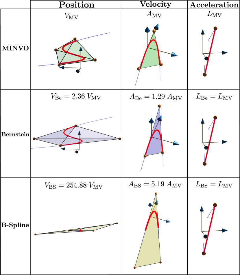
Figure 3: Comparison of the volumes, areas and lengths obtained by the MINVO basis (ours), Bernstein basis (used by the Bézier curves) and B-Spline basis for an interval ( ) of a given uniform B-Spline ( ). In the acceleration space, the three bases generate the same control points.

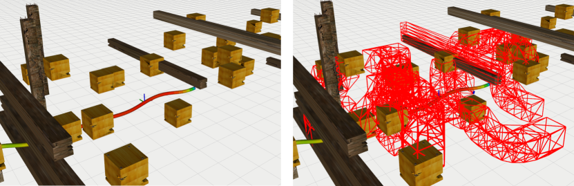
Figure 4: To impose collision-free constraints, MADER uses polyhedral representations of each interval of the trajectories of other agents/obstacles. On the left a given scenario with dynamic obstacles and on the right the polyhedral representations obtained (in red).

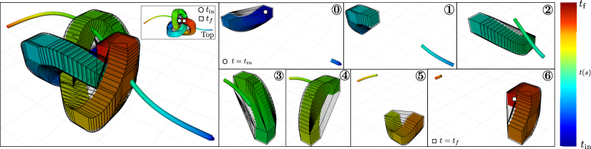
Figure 5: Example of a trajectory avoiding a dynamic obstacle. The obstacle has a box-like shape and is moving following a trefoil knot trajectory. The trajectory of the obstacle is divided into as many segments as the optimized trajectory has. An outer polyhedral representation (whose edges are shown as black lines) is computed for each of theses segments, and each segment of the trajectory avoids these polyhedra.

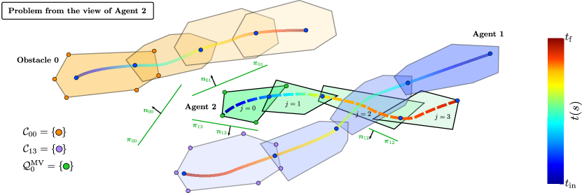
Figure 6: Collision-free constraints between agent 2 and both the obstacle 0 and agent 1. This figure is from the view of agent 2. $t_{\text{in}}$ and $t_{\text{f}}$ are the initial and final times of the trajectory being optimized (dashed lines), and they are completely independent of the initial and final optimization times of agent 1. $\mathcal{Q}_{0}^{\text{MV}}$ are the control points of the interval $0$ of the optimized trajectory using the MINVO basis. $\mathcal{C}_{13}$ are the vertexes of the convex hull of the vertexes of the control points of all the intervals of the trajectory of agent 1 that fall in $[t_{\text{f}}-\Delta t,t_{\text{f}}]$. Note that the trajectories and polyhedra are in 3D, but they are represented in 2D for visualization purposes.

IV-B Polyhedral Representation of the trajectory of other agents

We first increase the sides of $B_{i}$ by $\boldsymbol{\eta}_{s}$ to obtain the inflated box $B_{i}^{\prime}$. Now, note that the trajectory of the agent $i\neq s$ is also a B-Spline, but its initial and final times can be different from $t_{\text{in}}$ and $t_{\text{f}}$ (initial and final times of the trajectory that agent $s$ is optimizing). Therefore, to obtain the polyhedral representation of the trajectory of the agent $i$ in the intervals $[t_{\text{in}},t_{\text{in}}+\Delta t]$, $[t_{\text{in}}+\Delta t,t_{\text{in}}+2\Delta t]$, …, $[t_{\text{f}}-\Delta t,t_{\text{f}}]$ we first compute the MINVO control points of every interval of the trajectory of agent $i$ that falls in one of these intervals. The convex hull of the boxes $B_{i}^{\prime}$ placed in every one of these control points will be the polyhedral representation of the interval $j$ of the trajectory of the agent $i$. We denote the vertexes of this outer polyhedral representation as $\mathcal{C}_{ij}$.

IV-C Polyhedral Representation of the trajectory of the obstacles

For each interval $j$ we first increase the sides of $B_{i}$ by $\boldsymbol{\eta}_{s}+2(\boldsymbol{\beta}_{ij}+\boldsymbol{\alpha}_{ij})$, and denote this inflated box $B_{i}^{\prime}$. Here $\boldsymbol{\beta}_{ij}$ and $\boldsymbol{\alpha}_{ij}$ are the values defined in Sec. III. We then place $B_{i}^{\prime}$ in $\mathbf{p}_{i}(\mathcal{T}_{j})$, where $\mathbf{p}_{i}(\mathcal{T}_{j})$ denotes the set of positions of the obstacle $i$ at the times $\mathcal{T}_{j}$ (see Table I) and compute the convex hull of all the vertexes of these boxes. Given the first assumption of Sec. III, this guarantees that the convex hull obtained is an outer approximation of all the 3D space occupied by the obstacle $i$ (inflated by the size of the agent $s$) during the interval $j$. The static obstacles are treated in the same way, with $\mathbf{p}_{i}(t)=\text{constant}$. An example of these polyhedral representations is shown in Fig. 4.

V Optimization And Initial Guess

V-A Collision-free constraints

Once the polyhedral approximation of the trajectories of the other obstacles/agents have been obtained, we enforce the collision-free constraints between these polyhedra and the ones of the optimized trajectory as follows: we introduce the planes $\boldsymbol{\pi}_{ij}$ (characterized by $\boldsymbol{n}_{ij}$ and $d_{ij}$) that separate them as decision variables in the optimization problem and force this way the separation between the vertexes in $\mathcal{C}_{ij}$ and the MINVO control points $\mathcal{Q}_{j}^{\text{MV}}$ (see Figs. 5 and 6):

$$\boldsymbol{n}_{ij}^{T}\boldsymbol{c}+d_{ij}>0\quad\forall\boldsymbol{c}\in\mathcal{C}_{ij},\;\forall i\in I,j\in J$$ (3)

$$\boldsymbol{n}_{ij}^{T}\boldsymbol{q}+d_{ij}<0\quad\forall\boldsymbol{q}\in\mathcal{Q}_{j}^{\text{MV}},\;\forall j\in J$$

V-B Other constraints

The initial condition (position, velocity and acceleration) is imposed by $\mathbf{x}(t_{\text{in}})=\mathbf{x}_{in}$. Note that $\boldsymbol{p}_{\text{in}}$, $\boldsymbol{v}_{\text{in}}$ and $\boldsymbol{a}_{\text{in}}$ completely determine $\boldsymbol{q}_{0}$, $\boldsymbol{q}_{1}$ and $\boldsymbol{q}_{2}$, so these control points are not included as decision variables.

For the final condition, we use a final stop condition imposing the constraints $\mathbf{v}(t_{\text{f}})=\mathbf{v}_{f}=\boldsymbol{0}$ and $\mathbf{a}(t_{\text{f}})=\mathbf{a}_{f}=\boldsymbol{0}$. These conditions require $\boldsymbol{q}_{n-2}=\boldsymbol{q}_{n-1}=\boldsymbol{q}_{n}$, so the control points $\boldsymbol{q}_{n-1}$ and $\boldsymbol{q}_{n}$ can also be excluded from the set of decision variables. The final position is included as a penalty cost $\left\|\boldsymbol{q}_{n-2}-\boldsymbol{g}\right\|^{2}_{2}$ in the objective function, weighted with a parameter $\omega\geq 0$. Here $\boldsymbol{g}$ is the goal (projection of the $\boldsymbol{g}_{\text{term}}$ onto a sphere $\mathcal{S}$ of radius $r$ around $\boldsymbol{d}$, see Table I). Note that, as we are using clamped uniform B-Splines with a final stop condition, $\boldsymbol{q}_{n-2}$ coincides with the last position of the B-Spline. The reason of adding this penalty cost for the final position, instead of including $\boldsymbol{q}_{n-2}=\boldsymbol{g}$ as a hard constraint, is that a hard constraint can easily lead to infeasibility if the heuristics used for the total time $(t_{\text{f}}-t_{\text{in}})$ underestimates the time needed to reach $\boldsymbol{g}$.

To force the trajectory generated to be inside the sphere $\mathcal{S}$, we impose the constraint

$$\left\|\boldsymbol{q}-\boldsymbol{d}\right\|_{2}^{2}\leq r^{2}\qquad\forall\boldsymbol{q}\in\mathcal{Q}_{j}^{\text{MV}},\;\forall j\in J$$ (4)

Moreover, we also add the constraints on the maximum velocity and acceleration:

$$\qquad\text{abs}\left(\boldsymbol{v}\right)\leq\boldsymbol{v}_{\text{max}}\quad\forall\boldsymbol{v}\in\mathcal{V}_{j}^{\text{MV}},\;\forall j\in J$$ (5)

$$\qquad\text{abs}\left(\boldsymbol{a}_{l}\right)\leq\boldsymbol{a}_{\text{max}}\quad\forall l\in L\backslash\{n-1,n\}$$

where we are using the MINVO velocity control points for the velocity constraint. For the acceleration constraint, the B-Spline and MINVO control points are the same (see Fig. 3). Note that the velocity and acceleration are constrained independently on each one of the axes $\{x,y,z\}$.

V-C Control effort

The evaluation of a cubic clamped uniform B-Spline in an interval $j\in J$ can be done as follows [35]:

$$\mathbf{p}(t)=\boldsymbol{Q}_{j}^{\text{BS}}\boldsymbol{A}_{\text{pos}}^{\text{BS}}(j)\underbrace{\left[\begin{array}[]{c}u_{j}^{3}\\ u_{j}^{2}\\ u_{j}\\ 1\end{array}\right]}_{:=\boldsymbol{u}_{j}}$$

where $u_{j}:=\frac{t-t_{p+j}}{t_{p+j+1}-t_{p+j}}$, $t\in[t_{p+j},t_{p+j+1}]$ and $\boldsymbol{A}_{\text{pos}}^{\text{BS}}(j)$ is a known matrix that depends on each interval. Specifically, and with the knots chosen, we will have $\boldsymbol{A}_{\text{pos}}^{\text{BS}}(0)\neq\boldsymbol{A}_{\text{pos}}^{\text{BS}}(1)\neq\boldsymbol{A}_{\text{pos}}^{\text{BS}}(2)=...=\boldsymbol{A}_{\text{pos}}^{\text{BS}}(m-2p-3)\neq\boldsymbol{A}_{\text{pos}}^{\text{BS}}(m-2p-2)\neq\boldsymbol{A}_{\text{pos}}^{\text{BS}}(m-2p-1)$. Now, note that

$$\frac{d^{r}\mathbf{p}(t)}{dt^{r}}=\frac{1}{\Delta t^{r}}\boldsymbol{Q}_{j}^{\text{BS}}\boldsymbol{A}_{\text{pos}}^{\text{BS}}(j)\frac{d^{r}\boldsymbol{u}_{j}}{{du_{j}}^{r}}$$

Therefore, as the jerk is constant in each interval (since $p=3$), the control effort is:

$$\int_{t_{\text{in}}}^{t_{\text{f}}}\left\|\mathbf{j}(t)\right\|^{2}dt\propto\sum_{j\in J}\left\|\boldsymbol{Q}_{j}^{\text{BS}}\boldsymbol{A}_{\text{pos}}^{\text{BS}}(j)\left[\begin{array}[]{c}6\\ 0\\ 0\\ 0\end{array}\right]\right\|^{2}_{2}$$ (6)

V-D Optimization Problem

Given the constraints and the objective function explained above, the optimization problem solved is as follows:

$$\underset{\mathcal{Q}_{j}^{\text{BS}},\boldsymbol{n}_{ij},d_{ij}}{\boldsymbol{\min}}\sum_{j\in J}\left\|\boldsymbol{Q}_{j}^{\text{BS}}\boldsymbol{A}_{\text{pos}}^{\text{BS}}(j)\left[\begin{array}[]{c}6\\ 0\\ 0\\ 0\end{array}\right]\right\|^{2}_{2}+\omega\left\|\boldsymbol{q}_{n-2}-\boldsymbol{g}\right\|^{2}_{2}$$

s.t.

$$\quad\mathbf{x}(t_{\text{in}})=\mathbf{x}_{in}$$

$$\quad\mathbf{v}(t_{\text{f}})=\mathbf{v}_{f}=\boldsymbol{0}$$

$$\quad\mathbf{a}(t_{\text{f}})=\mathbf{a}_{f}=\boldsymbol{0}$$

$$\quad\boldsymbol{n}_{ij}^{T}\boldsymbol{c}+d_{ij}>0\quad\forall\boldsymbol{c}\in\mathcal{C}_{ij},\;\forall i,j$$

$$\quad\boldsymbol{n}_{ij}^{T}\boldsymbol{q}+d_{ij}<0\quad\forall\boldsymbol{q}\in\mathcal{Q}_{j}^{\text{MV}}:=f_{j}^{\text{BS}\rightarrow\text{MV}}(\mathcal{Q}_{j}^{\text{BS}}),\;\forall i,j$$

$$\quad\left\|\boldsymbol{q}-\boldsymbol{d}\right\|_{2}^{2}\leq r^{2}\quad\forall\boldsymbol{q}\in\mathcal{Q}_{j}^{\text{MV}}:=f_{j}^{\text{BS}\rightarrow\text{MV}}(\mathcal{Q}_{j}^{\text{BS}}),\;\forall j$$

$$\quad\text{abs}\left(\boldsymbol{v}\right)\leq\boldsymbol{v}_{\text{max}}\quad\forall\boldsymbol{v}\in\mathcal{V}_{j}^{\text{MV}}:=h_{j}^{\text{BS}\rightarrow\text{MV}}(\mathcal{Q}_{j}^{\text{BS}}),\;\forall j$$

$$\quad\text{abs}\left(\boldsymbol{a}_{l}\right)\leq\boldsymbol{a}_{\text{max}}\quad\forall l\in L\backslash\{n-1,n\}$$

This problem is clearly nonconvex since we are minimizing over the control points and the planes $\boldsymbol{\pi}_{ij}$ (characterized by $\boldsymbol{n}_{ij}$ and $d_{ij}$). Note also that the decision variables are the B-Spline control points $\mathcal{Q}_{j}^{\text{BS}}$. In the constraints, the MINVO control points $\mathcal{Q}_{j}^{\text{MV}}$ and $\mathcal{V}_{j}^{\text{MV}}$ are simply linear transformations of the decision variables (see Eq. 2). We solve this problem using the augmented Lagrangian method [36, 37], and with the globally-convergent method-of-moving-asymptotes (MMA) [38] as the subsidiary optimization algorithm. The interface used for these algorithms is NLopt [39]. The time allocated per trajectory is chosen before the optimization as $(t_{\text{f}}-t_{\text{in}})=\frac{\left\|\boldsymbol{g}-\boldsymbol{d}\right\|_{2}}{v_{max}}$.

V-E Initial Guess

1

2 Function GetInitialGuess():

3      

4      Compute $\boldsymbol{q}_{0}$, $\boldsymbol{q}_{1}$ and $\boldsymbol{q}_{2}$ from $\boldsymbol{p}_{\text{in}}$, $\boldsymbol{v}_{\text{in}}$ and $\boldsymbol{a}_{\text{in}}$

5      Add $\boldsymbol{q}_{2}$ to $Q$

6      while $Q$ is not empty do

7            

8            $\boldsymbol{q}_{l}\leftarrow$First element of $Q$

9            Remove first element of $Q$

10            $\mathcal{M}\leftarrow$Uniformly sample $\boldsymbol{v}_{l}$ satisfying $v_{max}$ and $a_{max}$

11            if any of the conditions 1-6 is true then

12                  

13                  continue

14            

15            if $\left\|\boldsymbol{q}_{l}-\boldsymbol{g}\right\|_{2}<\epsilon^{\prime\prime}$ and $l=(n-2)$ then

16                  

17                  $\boldsymbol{q}_{n-1}\leftarrow\boldsymbol{q}_{n-2}$

18                  $\boldsymbol{q}_{n}\leftarrow\boldsymbol{q}_{n-2}$

19                  return $\{\boldsymbol{q}_{0},\boldsymbol{q}_{1},\boldsymbol{q}_{2},\ldots,\boldsymbol{q}_{n-2},\boldsymbol{q}_{n-1},\boldsymbol{q}_{n}\}\cup\boldsymbol{\pi}_{ij}$

20                  

21            

22            for every $\boldsymbol{v}_{l}$ in $\mathcal{M}$ do

23                  

24                  $\boldsymbol{q}_{l+1}\leftarrow\boldsymbol{q}_{l}+\frac{t_{l+p+1}-t_{l+1}}{p}\boldsymbol{v}_{l}$

25                  Store in $\boldsymbol{q}_{l+1}$ a pointer to $\boldsymbol{q}_{l}$

26                  Add $\boldsymbol{q}_{l+1}$ to $Q$

27                  

28            

29      

30      return Closest Path found

Algorithm 1 Octopus Search

To obtain an initial guess (which consists of both the control points $\{\boldsymbol{q}_{0},\ldots,\boldsymbol{q}_{n}\}^{\text{BS}}$ and the planes $\boldsymbol{\pi}_{ij}$), we use the Octopus Search algorithm shown in Alg. 1. The Octopus Search takes inspiration from A^* [40], but it is designed to work with B-Splines, handle dynamic obstacles/agents, and use the MINVO basis for the collision check. Each control point will be a node in the search. All the open nodes are kept in a priority queue $Q$, in which the elements are ordered in increasing order of $f=g+\epsilon h$, where $g$ is the sum of the distances (between successive control points) from $\boldsymbol{q}_{0}$ to the current node (cost-to-come), $h$ is the distance from the current node to the goal (heuristics of the cost-to-go), and $\epsilon$ is the bias. Similar to A^*, this ordering of the priority queue makes nodes with lower $f$ be explored first.

The way the algorithm works is as follows: First, we compute the control points ${\boldsymbol{q}_{0},\;\boldsymbol{q}_{1},\;\boldsymbol{q}_{2}}$, which are determined from $\boldsymbol{p}_{\text{in}},\boldsymbol{v}_{\text{in}}$ and $\boldsymbol{a}_{\text{in}}$. After adding $\boldsymbol{q}_{2}$ to the queue $Q$ (line 1), we run the following loop until there are no elements in $Q$: First we store in $\boldsymbol{q}_{l}$ the first element of $Q$, and remove it from $Q$ (lines 1-1). Then, we store in a set $\mathcal{{M}}$ velocity samples for $\boldsymbol{v}_{l}$ that satisfy both $v_{\text{max}}$ and $a_{\text{max}}$. After this, we discard the current $\boldsymbol{q}_{l}$ if any of these conditions are true (l.s. denotes linearly separable):

1. $\mathcal{Q}_{l-3}^{\text{MV}}$ is not l.s. from $\mathcal{C}_{i,l-3}$ for some $i\in I$.

2. $l=(n-2)$ and $\mathcal{Q}_{n-4}^{\text{MV}}$ is not l.s. from $\mathcal{C}_{i,n-4}$ for some $i\in I$.

3. $l=(n-2)$ and $\mathcal{Q}_{n-3}^{\text{MV}}$ is not l.s. from $\mathcal{C}_{i,n-3}$ for some $i\in I$.

4. $\left\|\boldsymbol{q}_{l}-\boldsymbol{d}\right\|_{2}>r$.

5. $\left\|\boldsymbol{q}_{l}-\boldsymbol{q}_{k}\right\|_{\infty}\leq\epsilon^{\prime}$ for some $\boldsymbol{q}_{k}$ already added to $Q$.

6. Cardinality of $\mathcal{{M}}$ is zero.

Condition 1 ensures that the convex hull of $\mathcal{Q}_{l-3}^{\text{MV}}$ does not collide with any interval $l-3$ of other obstacle/agent $i\in I$. The linear separability is checked by solving the following feasibility linear problem for the interval $j=l-3$ of every obstacle/agent $i\in I$:

$$\begin{array}[]{cc}\boldsymbol{n}_{ij}^{T}\boldsymbol{c}+d_{ij}>0&\forall\boldsymbol{c}\in\mathcal{C}_{ij}\\ \boldsymbol{n}_{ij}^{T}\boldsymbol{q}+d_{ij}<0&\forall\boldsymbol{q}\in\mathcal{Q}_{j}^{\text{MV}}\end{array}$$ (7)

where the decision variables are the planes $\boldsymbol{\pi}_{ij}$ (defined by $\boldsymbol{n}_{ij}$ and $d_{ij}$). We solve this problem using GLPK [41]. Note that we also need to check the conditions 2 and 3 due to the fact that $\boldsymbol{q}_{n-2}=\boldsymbol{q}_{n-1}=\boldsymbol{q}_{n}$ and hence the choice of $\boldsymbol{q}_{n-2}$ in the search forces the choice of $\boldsymbol{q}_{n-1}$ and $\boldsymbol{q}_{n}$. In all these three previous conditions, the MINVO control points are used.

As in the optimization problem we are imposing the trajectory to be inside the sphere $\mathcal{S}$, we also discard $\boldsymbol{q}_{l}$ if condition 4 is not satisfied. Additionally, to keep the search computationally tractable, we discard $\boldsymbol{q}_{l}$ if it is very close to another $\boldsymbol{q}_{k}$ already added to $Q$ (condition 5): we create a voxel grid of voxel size $2\epsilon^{\prime}$, and add a new control point to $Q$ only if no other point has been added before within the same voxel. Finally, we also discard $\boldsymbol{q}_{l}$ if there are not any feasible samples for $\boldsymbol{v}_{l}$ (condition 6).

Then, we check if we have found all the control points and if $\boldsymbol{q}_{n-2}$ is sufficiently close to the goal $\boldsymbol{g}$ (distance less than $\epsilon^{\prime\prime}$). If this is the case, the control points $\boldsymbol{q}_{n-1}$ and $\boldsymbol{q}_{n}$ (which are the same as $\boldsymbol{q}_{n-2}$ due to the final stop condition) are added to the list of the corresponding control points, and are returned together with all the separating planes $\boldsymbol{\pi}_{ij}\;\forall i\in I,\forall j\in J$ (lines 1-1). If the goal has not been reached yet, we use the velocity samples $\mathcal{M}$ to generate $\boldsymbol{q}_{l+1}$ and add them to $Q$ (lines 1-1). If the algorithm is not able to find a trajectory that reaches the goal, the one found that is closest to the goal is returned (line 1).

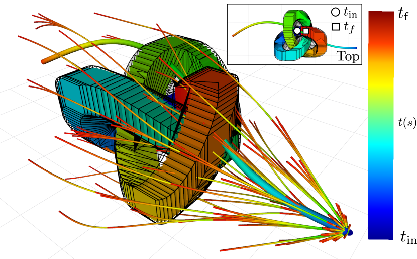
Figure 7: Example of the trajectories found by the Octopus Search in an environment with a dynamic obstacle following a trefoil knot trajectory. The best trajectory found is the thickest one in the figure.

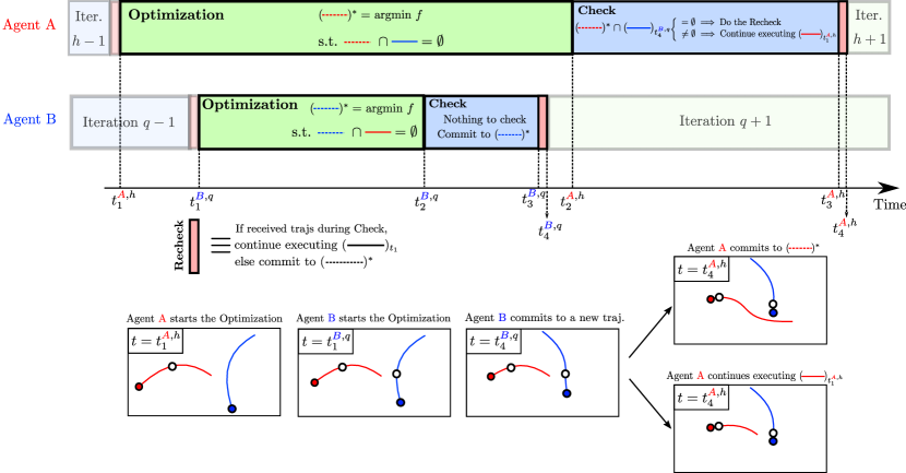
Figure 8: Deconfliction between agents. Each agent includes the trajectories other agents have committed to as constraints in the optimization. After the optimization, a collision check-recheck scheme is performed to ensure feasibility with respect to trajectories other agents have committed to while the optimization was happening. In this example, agent B starts the optimization after agent A, but commits to a trajectory before agent A. Hence, when agent A finishes the optimization it needs to check whether the trajectory found collides or not with the trajectory agent B committed to at $t=t_{4}^{{\color[rgb]{0,0,1}B},q}$. If it collides, agent A will simply keep executing the trajectory available at $t=t_{1}^{{\color[rgb]{1,0,0}A},h}$. If it does not collide, agent A will do the Recheck step to ensure no agent has committed to any trajectory during the Check period, and if this Recheck step is satisfied, agent A will commit to the trajectory found.

Fig. 7 shows an example of the trajectories found by the Octopus Search algorithm in an environment with a dynamic obstacle following a trefoil knot trajectory.

V-F Degree of the splines

In this paper, we focused on the case $p=3$ (i.e., cubic splines). However, MADER could also be used with higher (or lower) order splines. For instance, one could use splines of fourth-degree polynomials (i.e., $p=4$), minimize snap (instead of jerk), and then use the corresponding MINVO polyhedron that encloses each fourth-degree interval for the obstacle avoidance constraints [1]. The reason behind the choice of cubic splines, instead of higher/lower order splines, is that cubic splines are a good trade-off between dynamic feasibility of a UAV [42] and computational tractability.

VI Deconfliction

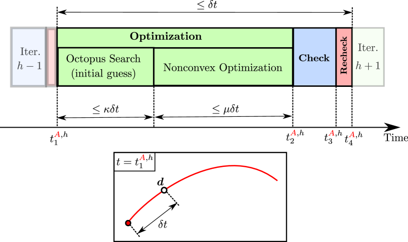
Figure 9: At $t=t_{1}^{{\color[rgb]{1,0,0}A},h}$, agent A chooses the point $\boldsymbol{d}$ ( ) along the current trajectory that it is executing, with an offset $\delta t$ from the current position . Then, it allocates $\kappa\delta t$ seconds to obtain an initial guess. The closest trajectory found to $\boldsymbol{g}$ is used as the initial guess if the search has not finished by that time. Then, the nonconvex optimization runs for $\mu\delta t$ seconds, choosing the best feasible solution found if no local optimum has been found by then. $\kappa$ and $\mu$ satisfy $\kappa>0$, $\mu>0$, $\kappa+\mu<1$.

To guarantee that the agents plan trajectories asynchronously while not colliding with other agents that are also constantly replanning, we use a deconfliction scheme divided in these three periods (see Fig. 8):

• The Optimization period happens during $t\in(t_{1},t_{2}]$. The optimization problem will include the polyhedral outer representations of the trajectories $p_{i}(t),\;i\in I$ in the constraints. All the trajectories other agents commit to during the Optimization period are stored.

• The Check happens during $t\in(t_{2},t_{3}]$. The goal of this period is to check whether the trajectory found in the optimization collides with the trajectories other agents have committed to during the optimization. This collision check is done by performing feasibility tests solving the Linear Program 7 $\forall j$ for every agent $i$ that has committed to a trajectory while the optimization was being performed (and whose new trajectory was not included in the constraints at $t_{1}$). A boolean flag is set to true if any other agent commits to a new trajectory during this Check period.

• The Recheck period aims at checking whether agent A has received any trajectory during the Check period, by simply checking if the boolean flag is true or false. As this is a single Boolean comparison in the code, it allows us to assume that no trajectories have been published by other agents while this recheck is done, avoiding therefore an infinite loop of rechecks.

With $h$ denoting the replanning iteration of an agent A, the time allocation for each of these three periods described above is explained in Fig. 9: to choose the initial condition of the iteration $h$, Agent A first chooses a point $\boldsymbol{d}$ along the trajectory found in the iteration $h-1$, with an offset of $\delta t$ seconds from the current position . Here, $\delta t$ should be an estimate of how long iteration $h$ will take. To obtain this estimate, and similar to our previous work [10], we use the time iteration $h-1$ took multiplied by a factor $\alpha\geq 1$: $\delta t=\alpha\left(t_{4}^{{\color[rgb]{1,0,0}A},h-1}-t_{1}^{{\color[rgb]{1,0,0}A},h-1}\right)$. Agent A then should finish the replanning iteration $h$ in less than $\delta t$ seconds. To do this, we allocate a maximum runtime of $\kappa\delta t$ seconds to obtain an initial guess, and a maximum runtime of $\mu\delta t$ seconds for the nonconvex optimization. Here $\kappa>0,\mu>0$ and $\kappa+\mu<1$, to give time for the Check and Recheck. If the Octopus Search takes longer than $\kappa\delta t$, the trajectory found that is closest to the goal is used as the initial guess. Similarly, if the nonconvex optimization takes longer than $\mu\delta t$, the best feasible solution found is selected.

Fig. 8 shows an example scenario with only two agents A and B. Agent A starts its $h$-th replanning step at $t_{1}^{{\color[rgb]{1,0,0}A},h}$, and finishes the optimization at $t_{2}^{{\color[rgb]{1,0,0}A},h}$. Agent B starts its $q$-th replanning step at $t_{1}^{{\color[rgb]{0,0,1}B},q}$. In the example shown, agent B starts the optimization later than agent A ($t_{1}^{{\color[rgb]{0,0,1}B},q}>t_{1}^{{\color[rgb]{1,0,0}A},h}$), but solves the optimization earlier than agent A ($t_{2}^{{\color[rgb]{0,0,1}B},q}<t_{2}^{{\color[rgb]{1,0,0}A},h}$). As no other agent has obtained a trajectory while agent B was optimizing, agent B does not have to check anything, and commits directly to the trajectory found. However, when agent A finishes the optimization at $t_{2}^{{\color[rgb]{1,0,0}A},h}>t_{4}^{{\color[rgb]{0,0,1}B},q}$, it needs to check if the trajectory found collides with the one agent B has committed to. If they do not collide, agent A will perform the Recheck by ensuring that no trajectory has been published while the Check was being performed.

An agent will keep executing the trajectory found in the previous iteration if any of these four scenarios happens:

1. The trajectory obtained at the end of the optimization collides with any of the trajectories received during the Optimization.

2. The agent has received any trajectory from other agents during the Check period.

3. No feasible solution has been found in the Optimization.

4. The current iteration takes longer than $\delta t$ seconds.

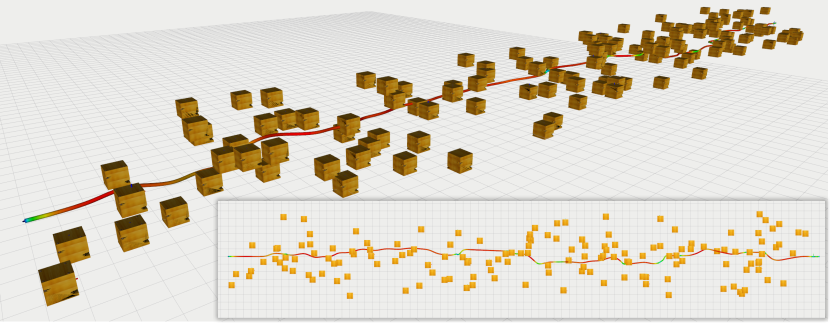
Figure 10: Corridor environment of size $73\;\text{m}\times 4\;\text{m}\times 3\;\text{m}$ used for the single-agent simulation. It contains 100 randomly-deployed dynamic obstacles that follow a trefoil knot trajectory. The corridor is along the $x$ direction.

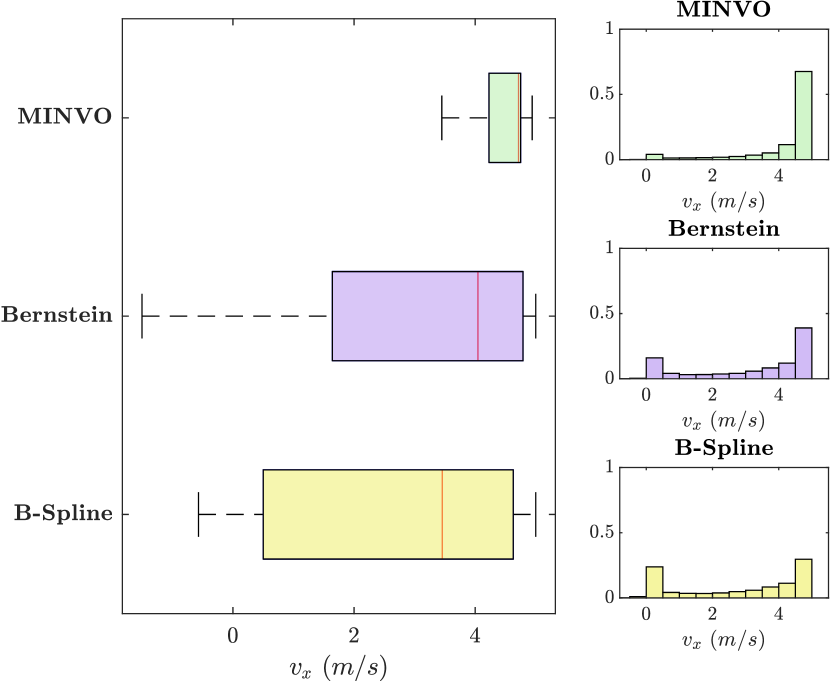
Figure 11: Boxplots and normalized histograms of the velocity profile of $v_{x}$ in the corridor environment shown in Fig. 10. The velocity constraint used was $\boldsymbol{v}_{max}=5\cdot\boldsymbol{1}\;m/s$. The histograms are for all the velocities obtained across 10 different simulations.

Under the third assumption explained in Sec. III (i.e., two agents do not commit to their trajectory at the very same time), this deconfliction scheme explained guarantees safety with respect to the other agents, which is proven as follows:

• If the planning agent commits to a new trajectory in the current replanning iteration, this new trajectory is guaranteed to be collision-free because it included all the trajectories of other agents as constraints, and it was checked for collisions with respect to the trajectories other agents have committed to during the planning agent’s optimization time.

• If the planning agent does not commit to a new trajectory in that iteration (because one of the scenarios 1–4 occur), it will keep executing the trajectory found in the previous iteration. This trajectory is still guaranteed to be collision-free because it was collision-free when it was obtained and other agents have included it as a constraint in any new plans that have been made recently. If the agent reaches the end of this trajectory (which has a final stop condition), the agent will wait there until it obtains a new feasible solution. In the meanwhile, all the other agents are including its position as a constraint for theirs trajectories, guaranteeing therefore safety between the agents.

VII Results

We now test MADER in several single-agent and multi-agent simulation environments. The computers used for the simulations are an AlienWare Aurora r8 desktop (for the C++ simulations of VII-B), a ROG Strix GL502VM laptop (for the Matlab simulations of Sec. VII-B) and a general-purpose-N1 Google Cloud instance (for the simulations of Sec. VII-A and VII-C).

VII-A Single-Agent simulations

To highlight the benefits of the MINVO basis with respect to the Bernstein or B-Spline bases, we first run the algorithm proposed in a corridor-like enviroment ($73\;\text{m}\times 4\;\text{m}\times 3\;\text{m}$) depicted in Fig. 10. that contains 100 randomly-deployed dynamic obstacles of sizes $0.8\;\text{m}\times 0.8\;\text{m}\times 0.8\;\text{m}$. All the obstacles follow a trajectory whose parametric equations are those of a trefoil knot [43]. The radius of the sphere $\mathcal{S}$ used is $r=4.0$ m, and the velocity and acceleration constraints for the UAV are $\boldsymbol{v}_{max}=5\cdot\boldsymbol{1}\;m/s$ and $\boldsymbol{a}_{max}=\left[\begin{array}[]{ccc}20&20&9.6\end{array}\right]^{T}\;m/s^{2}$. The velocity profile for $v_{x}$ is shown in Fig. 11. For the same given velocity constraint ($v_{\text{max}}=5\;m/s$), the mean velocity $v_{x}$ achieved by the MINVO basis is $4.15\;m/s$, higher than the ones achieved by the Bernstein and B-Spline basis ($3.23\;m/s$ and $2.79\;m/s$ respectively).

Table III: Comparison of the number of stops and time to reach the goal in a corridor-like environment using different bases and with different number of obstacles.

	50 obstacles		100 obstacles		150 obstacles		200 obstacles		250 obstacles
Basis	Stops	Time (s)	Stops	Time (s)	Stops	Time (s)	Stops	Time (s)	Stops	Time (s)
B-Spline	$4.6\pm 2.50$	$19.61\pm 1.67$	$9.0\pm 2.40$	$26.17\pm 3.04$	$9.1\pm 2.31$	$26.97\pm 3.24$	$12.1\pm 2.77$	$32.69\pm 4.61$	$14.10\pm 4.09$	$39.81\pm 9.76$
Bernstein	$5.0\pm 2.0$	$19.07\pm 1.08$	$7.4\pm 2.36$	$22.59\pm 1.33$	$6.5\pm 1.72$	$23.23\pm\boldsymbol{1.43}$	$7.2\pm 2.49$	$24.65\pm 2.54$	$8.4\pm\boldsymbol{2.80}$	$27.94\pm 4.16$
MINVO (ours)	$\boldsymbol{1.1\pm 0.74}$	$\boldsymbol{16.62\pm 0.61}$	$\boldsymbol{1\pm 0.94}$	$\boldsymbol{17.55\pm 0.98}$	$\boldsymbol{2.7\pm 1.70}$	$\boldsymbol{20.48}\pm 2.26$	$\boldsymbol{4.2\pm 1.87}$	$\boldsymbol{22.47\pm 2.19}$	$\boldsymbol{8.1}\pm 3.45$	$\boldsymbol{27.78\pm 3.83}$

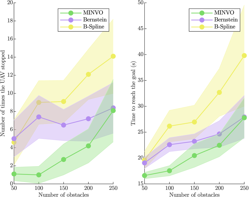
Figure 12: Time to reach the goal and number of times the UAV had to stop for different number of obstacles. 5 simulations were performed for each combination of basis (MINVO, Bernstein and B-Spline) and number of obstacles. The shaded area is the 1$\sigma$ interval, where $\sigma$ is the standard deviation.

We now compare the time it takes for the UAV to reach the goal using each basis in the same corridor environment but varying the total number of obstacles (from 50 obstacles to 250 obstacles). Moreover, and as a stopping condition is not a safe condition in a world with dynamic obstacles, we also report the number of times the UAV had to stop. The results are shown in Table III and Fig. 12. In terms of number of stops, the use of the MINVO basis achieves reductions of 86.4% and 88.8% with respect to the Bernstein and B-Spline bases respectively. In terms of the time to reach the goal, the MINVO basis achieves reductions of 22.3% and 33.9% compared to the Bernstein and B-Spline bases respectively. The reason behind all these improvements is the tighter outer polyhedral approximation of each interval of the trajectory achieved by the MINVO basis in the velocity and position spaces.

VII-B Multi-Agent simulations without obstacles

We now compare MADER with the following different state-of-the-art algorithms:

• Sequential convex programming (SCP, [23]).

• Relative Bernstein Polynomial approach (RBP, [27]).

• Distributed model predictive control (DMPC, [31]).

• Decoupled incremental sequential convex programming (dec_iSCP,[28]).

• Search-based motion planing ([32]), both in its sequential version (decS_Search) and in its non-sequential version (decNS_Search).

To classify these different algorithms, we use the following definitions:

• Decentralized: Each agent solves its own optimization problem.

• Replanning: The agents have the ability to plan several times as they fly (instead of planning only once before starting to fly). The algorithms with replanning are also classified according to whether they satisfy the real-time constraint in the replanning: algorithms that satisfy this constraint are able to replan in less than $\delta t$ or at least have a trajectory they can keep executing in case no solution has found by then (see Fig. 9). Algorithms that do not satisfy this constraint allow replanning steps longer than $\delta t$ (which is not feasible in the real world), and simulations are performed by simply having a simulation time that runs completely independent of the real time.

• Asynchronous: The planning is triggered independently by each agent without considering the planning status of other agents. Examples of synchronous algorithms include the ones that trigger the optimization of all the agents at the same time or that impose that one agent cannot plan until another agent has finished.

• Discretization for inter-agent constraints: The collision-free constraints between the agents are imposed only on a finite set of points of the trajectories. The discretization step will be denoted as $h$ seconds.

In the test scenario, 8 agents are in a $8\times 8$ m square, and they have to swap their positions. The velocity and acceleration constraints used are $\boldsymbol{v}_{max}=1.7\cdot\boldsymbol{1}\;m/s$ and $a_{max}=6.2\cdot\boldsymbol{1}\;m/s^{2}$, with a drone radius of 15 cm. Moreover, we define the safety ratio as $\min_{i,i^{{}^{\prime}}}d_{min}^{i,i^{\prime}}/(\rho_{i}+\rho_{i^{\prime}})$ [27], where $d_{min}^{i,i^{\prime}}$ is the minimum distance over all the pairs of agents $i$ and $i^{\prime}$, and $\rho_{i}$, $\rho_{i^{\prime}}$ denote their respective radii. Safety is ensured if safety ratio $>1$. For the RBP and DMPC algorithms, the downwash coefficient $c$ was set to $c=1$ (so that the drone is modeled as a sphere as in all the other algorithms).

Table IV: Comparison between MADER (ours), SCP ([23]), RBP ([27]), DMPC ([31]), dec_iSCP ([28]), decS_Search and decNS_Search ([32]) . For SCP and MADER, the time and distance results are the mean of 5 runs, and the safety ratio is the minimum across all the runs. The test environment consists of 8 agents in a square that swap their positions without obstacles. For the algorithms that have replanning, the values in the columns of computation and execution times are $t_{1^{st}\text{start}}$ | $t_{\text{last start}}$ | $t_{1^{st}\text{end}}$ (see Fig. 13). The superscript ^∗ means the available implementation of the algorithm is in MATLAB (rest is in C++). Algorithms that have replanning but do not satisfy the real-time constraints in the replanning are denoted as Yes/No in the Replan? column of the table.

Method	Decentr.?	Replan?	Async.?	Without discretization?	Time (s)			Total Flight Distance (m)	Safety
					Computation	Execution	Total		Safe?	Safety ratio
SCP, $h_{\text{SCP}}=0.3$ s					1.150	7.215	8.366	77.144	No	0.142
SCP, $h_{\text{SCP}}=0.25$ s					3.099	7.855	10.954	101.733	No	0.149
SCP, $h_{\text{SCP}}=0.2$ s					8.741	7.855	16.596	90.917	No	0.335
SCP, $h_{\text{SCP}}=0.17$ s	No	No	No	No	37.375	9.775	47.150	77.346	No	0.685
RBP, batch_size=1					0.228	15.623	15.851	90.830	Yes	1.055
RBP, batch_size=2					0.236	15.623	15.859	91.789	Yes	1.075
RBP, batch_size=4					0.277	14.203	14.480	92.133	Yes	1.023
RBP, no batches	No	No	No	Yes	0.461	14.203	14.664	93.721	Yes	1.057
DMPC∗, $h_{\text{DMPC}}=0.45$ s					4.952	23.450	28.402	79.650	No	0.683
DMPC∗, $h_{\text{DMPC}}=0.36$ s					4.350	20.710	25.060	97.220	No	0.914
DMPC∗, $h_{\text{DMPC}}=0.3$ s					4.627	18.430	23.057	78.580	Yes	1.015
DMPC∗, $h_{\text{DMPC}}=0.25$ s	Yes	No	No	No	3.796	15.980	19.776	79.590	No	0.824
dec_iSCP∗, $h_{\text{iSCP}}=0.4$ s					2.631	13.130	15.761	102.320	No	0.017
dec_iSCP∗, $h_{\text{iSCP}}=0.3$ s					4.276	15.470	19.746	97.770	No	0.550
dec_iSCP∗, $h_{\text{iSCP}}=0.2$ s					9.639	14.060	23.699	95.790	No	0.917
dec_iSCP∗, $h_{\text{iSCP}}=0.15$ s	Yes	No	No	No	14.138	14.060	28.198	102.030	No	0.906
decS_Search, $u=2\;m/s^{3}$					15.336	6.491	21.827	79.354	Yes	1.337
decS_Search, $u=3\;m/s^{3}$					7.772	6.993	14.764	80.419	Yes	1.768
decS_Search, $u=4\;m/s^{3}$					34.557	9.491	44.048	83.187	Yes	1.491
decS_Search, $u=5\;m/s^{3}$	Yes	No	No	Yes	3.104	8.491	11.595	80.804	Yes	1.474
decNS_Search, $u=2\;m/s^{3}$					0.021 | 0.233 | 33.711		34.288	80.116	Yes	1.416
decNS_Search, $u=3\;m/s^{3}$					0.003 | 0.058 | 12.810		13.346	79.752	Yes	1.150
decNS_Search, $u=4\;m/s^{3}$					0.030 | 0.600 | 53.824		53.899	79.752	Yes	1.502
decNS_Search, $u=5\;m/s^{3}$	Yes		No	Yes	0.002 | 0.051 | 9.096		9.169	88.753	Yes	1.335
MADER (ours)	Yes	Yes	Yes	Yes	0.550 | 2.468 | 7.975		10.262	82.487	Yes	1.577

The results obtained, together with the classification of each algorithm, are shown in Table IV. For the algorithms that replan as they fly, we show the following times (see Fig. 13): $t_{1^{st}\text{start}}$ (earliest time a UAV starts flying), $t_{\text{last start}}$ (latest time a UAV starts flying), $t_{1^{st}\text{end}}$ (earliest time a UAV reaches the goal) and the total time $t_{\text{total}}$ (time when all the UAVs have reached their goals). Note that the algorithm decNS_Search is synchronous (link), and it does not satisfy the real-time constraints in the replanning iterations (link). Several conclusions can be drawn from Table IV:

• Algorithms that use discretization to impose inter-agent constraints are in general not safe due to the fact that the constraints may not be satisfied between two consecutive discretization points. A smaller discretization step may solve this, but at the expense of very high computation times.

• Compared to the centralized solution that generates safe trajectories (RBP), MADER achieves a shorter overall flight distance. The total time of MADER is also shorter than the one of RBP.

• Compared to decentralized algorithms (DMPC, dec_iSCP, decS_Search and decNS_Search), MADER is the one with the shortest total time, except for the case of decNS_Search with $u=5\;m/s^{3}$. However, for this case the flight distance achieved by MADER is $6.3$ m shorter. Moreover, MADER is asynchronous and satisfies the real-time constraints in the replanning, while decNS_Search does not.

• From all the algorithms shown in Table IV, MADER is the only algorithm that is decentralized, has replanning, satisfies the real-time constraints in the replanning and is asynchronous.

Figure 13: Time notation for the algorithms that have replanning.

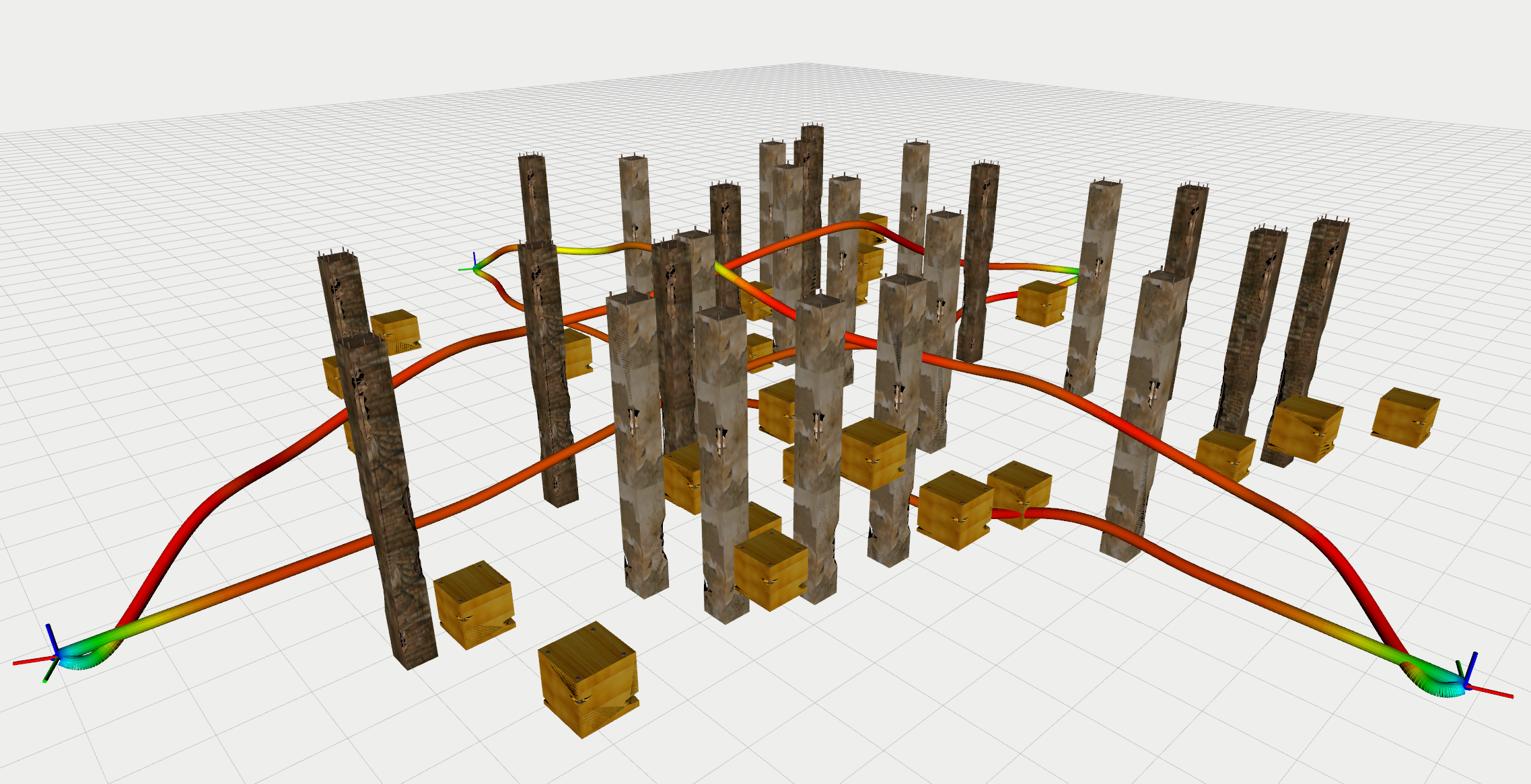
(a) 4 agents

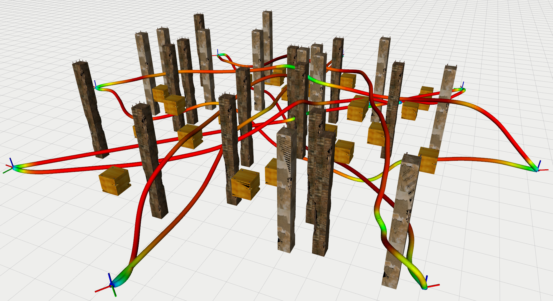
(b) 8 agents

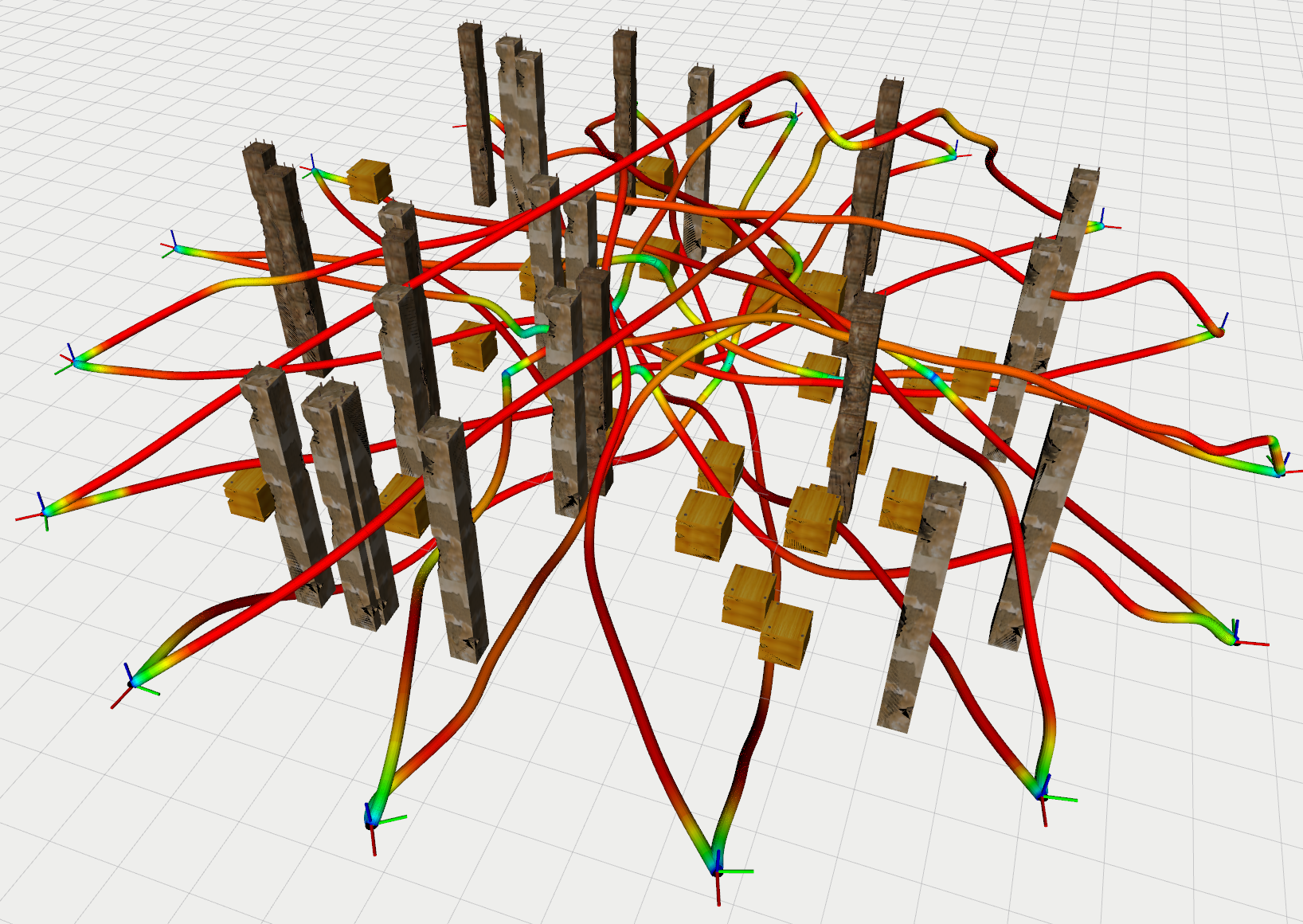
(c) 16 agents

Figure 14: Results for the circle environment, that contains 25 static obstacles (pillars) and 25 dynamic obstacles (boxes). The case with 32 agents is shown in Fig. 1a.

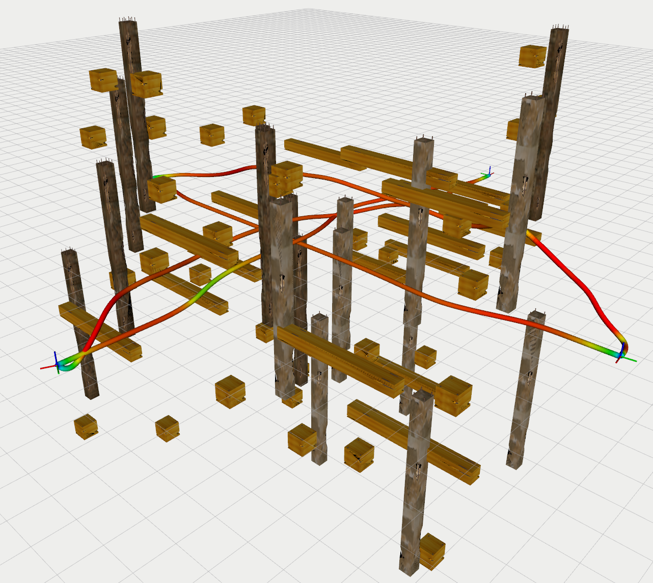
(a) 4 agents.

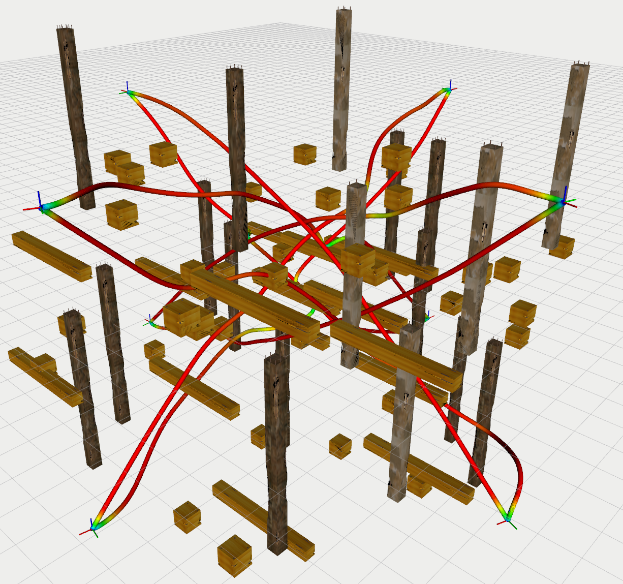
(b) 8 agents.

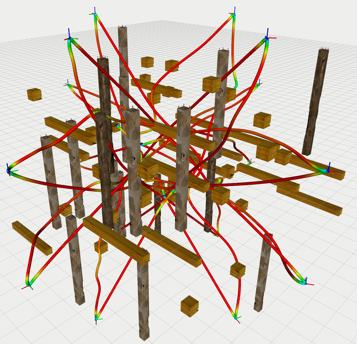
(c) 16 agents.

Figure 15: Results for the sphere environment, that contains 18 static obstacles (pillars) and 52 dynamic obstacles (boxes and horizontal poles). The case with 32 agents is shown in Fig. 1b.

Table V: Results for MADER in the circle and sphere environments.

Environment	Num of Agents	Time (s)				Flight Distance per agent (m)	Safety ratio between agents	Number of stops per agent
		$t_{1^{st}\text{start}}$	$t_{\text{last start}}$	$t_{1^{st}\text{end}}$	Total
Circle	4	0.339	0.563	10.473	11.403	21.052	5.444	0.000
	8	0.404	0.559	7.544	11.108	21.025	1.959	0.000
	16	0.300	0.764	7.773	13.972	21.737	4.342	0.188
	32	0.532	1.195	9.092	18.820	22.105	1.834	1.500
Sphere	4	0.452	0.584	10.291	11.124	20.827	4.242	0.000
	8	0.425	0.618	9.204	12.561	21.684	1.903	0.125
	16	0.363	0.845	8.909	13.175	21.284	1.905	0.125
	32	0.357	1.725	9.170	18.275	22.284	1.155	1.000

For MADER, and measured on the simulation environment used in this Section, each UAV performs on average 12 successful replans before reaching the goal. On average, the check step takes $\approx 2.87$ ms, the recheck step takes $\approx 0.034$ $\mu$s, and the total replanning time is $\approx 199.6$ ms. Approximately half of this replanning time is allocated to find the initial guess (i.e., $\kappa=0.5$).

VII-C Multi-Agent simulations with static and dynamic obstacles

We now test MADER in multi-agent environments that have also static and dynamic obstacles. For this set of experiments, we use $\boldsymbol{\alpha}_{j}=\boldsymbol{\beta}_{j}=3\cdot\boldsymbol{1}$ cm, $\gamma_{j}=0.1$ s $\forall j$, $r=4.5$ m (radius of the sphere $\mathcal{S}$), and a drone radius of $5$ cm. We test MADER in the following two environments:

• Circle environment: the UAVs start in a circle formation and have to swap their positions while flying in a world with 25 static obstacles of size $0.4\;\text{m}\times 8\;\text{m}\times 0.4\;\text{m}$ and 25 dynamic obstacles of size $0.6\;\text{m}\times 0.6\;\text{m}\times 0.6\;\text{m}$ following a trefoil knot trajectory [43]. The radius of the circle the UAVs start from is $10$ m.

• Sphere environment: the UAVs start in a sphere formation and have to swap their positions while flying in a world with 18 static obstacles of size $0.4\;\text{m}\times 8\;\text{m}\times 0.4\;\text{m}$, 17 dynamic obstacles of size $0.4\;\text{m}\times 4\;\text{m}\times 0.4\;\text{m}$ (moving in $z$) and 35 dynamic obstacles of size $0.6\;\text{m}\times 0.6\;\text{m}\times 0.6\;\text{m}$ following a trefoil knot trajectory. The radius of the sphere the UAVs start from is $10$ m.

The results can be seen in Table V and in Figs. 1, 14 and 15. All the safety ratios between the agents are $>1$, and the flight distances achieved (per agent) are approximately $21.5$ m. With respect to the number of stops, none of the UAVs had to stop in the circle environment with 4 and 8 agents and in the sphere environment with 4 agents. For the circle environment with 16 and 32 agents, each UAV stops (on average) 0.188 and 1.5 times respectively. For the sphere environment with 8, 16, and 32 agents, each UAV stops (on average) 0.125, 0.125, and 1.0 times respectively.
Note also that only the two agents that have been the closest are the ones that determine the actual value of the safety ratio, while the other agents do not contribute to this value. This means that, while the safety ratio is likely to decrease with the number of agents, a monotonic decrease of the safety ratio with respect to the number of agents is not strictly required.

VIII Conclusions

This work presented MADER, a decentralized and asynchronous planner that handles static obstacles, dynamic obstacles and other agents. By using the MINVO basis, MADER obtains outer polyhedral representations of the trajectories that are 2.36 and 254.9 times smaller than the volumes achieved using the Bernstein and B-Spline bases. To ensure non-conservative, collision-free constraints with respect to other obstacles and agents, MADER includes as decision variables the planes that separate each pair of outer polyhedral representations. Safety with respect to other agents is guaranteed in a decentralized and asynchronous way by including their committed trajectories as constraints in the optimization and then executing a collision check-recheck scheme. Extensive simulations in dynamic multi-agent environments have highlighted the improvements of MADER with respect to other state-of-the-art algorithms in terms of number of stops, computation/execution time and flight distance. Future work includes adding perception-aware and risk-aware terms in the objective function, as well as hardware experiments.

IX Acknowledgements

The authors would like to thank Pablo Tordesillas, Michael Everett, Dr. Kasra Khosoussi, Andrea Tagliabue and Parker Lusk for helpful insights and discussions. Thanks also to Andrew Torgesen, Jeremy Cai, and Stewart Jamieson for their comments on the paper. Research funded in part by Boeing Research & Technology.

Jesus Tordesillas (Student Member, IEEE) received the B.S. and M.S. degrees in Electronic engineering and Robotics from the Technical University of Madrid (Spain) in 2016 and 2018 respectively. He then received his M.S. in Aeronautics and Astronautics from MIT in 2019. He is currently pursuing the PhD degree with the Aeronautics and Astronautics Department, as a member of the Aerospace Controls Laboratory (MIT) under the supervision of Jonathan P. How. His research interests include path planning for UAVs in unknown environments and optimization. His work was a finalist for the Best Paper Award on Search and Rescue Robotics in IROS 2019.

Jonathan P. How (Fellow, IEEE) received the B.A.Sc. degree from the University of Toronto (1987), and the S.M. and Ph.D. degrees in aeronautics and astronautics from MIT (1990 and 1993). Prior to joining MIT in 2000, he was an Assistant Professor at Stanford University. He is currently the Richard C. Maclaurin Professor of aeronautics and astronautics at MIT. Some of his awards include the IEEE CSS Distinguished Member Award (2020), AIAA Intelligent Systems Award (2020), IROS Best Paper Award on Cognitive Robotics (2019), and the AIAA Best Paper in Conference Awards (2011, 2012, 2013). He was the Editor-in-chief of IEEE Control Systems Magazine (2015–2019), is a Fellow of AIAA, and was elected to the National Academy of Engineering in 2021.

References

- [1] J. Tordesillas and J. How, “MINVO basis: Finding simplexes with minimum volume enclosing polynomial curves,” arXiv preprint, 2020.
- [2] X. Zhou, Z. Wang, C. Xu, and F. Gao, “Ego-planner: An esdf-free gradient-based local planner for quadrotors,” arXiv preprint arXiv:2008.08835, 2020.
- [3] N. Bucki, J. Lee, and M. W. Mueller, “Rectangular pyramid partitioning using integrated depth sensors (rappids): A fast planner for multicopter navigation,” arXiv preprint arXiv:2003.01245, 2020.
- [4] B. Zhou, J. Pan, F. Gao, and S. Shen, “Raptor: Robust and perception-aware trajectory replanning for quadrotor fast flight,” arXiv preprint arXiv:2007.03465, 2020.
- [5] P. Florence, J. Carter, and R. Tedrake, “Integrated perception and control at high speed: Evaluating collision avoidance maneuvers without maps,” in Workshop on the Algorithmic Foundations of Robotics (WAFR), 2016.
- [6] P. R. Florence, J. Carter, J. Ware, and R. Tedrake, “Nanomap: Fast, uncertainty-aware proximity queries with lazy search over local 3d data,” in 2018 IEEE International Conference on Robotics and Automation (ICRA). IEEE, 2018, pp. 7631–7638.
- [7] B. T. Lopez and J. P. How, “Aggressive 3-D collision avoidance for high-speed navigation,” in Robotics and Automation (ICRA), 2017 IEEE International Conference on. IEEE, 2017, pp. 5759–5765.
- [8] ——, “Aggressive collision avoidance with limited field-of-view sensing,” in Intelligent Robots and Systems (IROS), 2017 IEEE/RSJ International Conference on. IEEE, 2017, pp. 1358–1365.
- [9] J. Tordesillas, B. T. Lopez, J. Carter, J. Ware, and J. P. How, “Real-time planning with multi-fidelity models for agile flights in unknown environments,” in 2019 IEEE International Conference on Robotics and Automation (ICRA). IEEE, 2019.
- [10] J. Tordesillas, B. T. Lopez, and J. P. How, “FASTER: Fast and safe trajectory planner for flights in unknown environments,” in 2019 IEEE/RSJ International Conference on Intelligent Robots and Systems (IROS). IEEE, 2019.
- [11] J. Chen, T. Liu, and S. Shen, “Online generation of collision-free trajectories for quadrotor flight in unknown cluttered environments,” in Robotics and Automation (ICRA), 2016 IEEE International Conference on. IEEE, 2016, pp. 1476–1483.
- [12] F. Gao, W. Wu, W. Gao, and S. Shen, “Flying on point clouds: Online trajectory generation and autonomous navigation for quadrotors in cluttered environments,” Journal of Field Robotics, vol. 36, no. 4, pp. 710–733, 2019.
- [13] B. Zhou, F. Gao, L. Wang, C. Liu, and S. Shen, “Robust and efficient quadrotor trajectory generation for fast autonomous flight,” IEEE Robotics and Automation Letters, vol. 4, no. 4, pp. 3529–3536, 2019.
- [14] H. Oleynikova, M. Burri, Z. Taylor, J. Nieto, R. Siegwart, and E. Galceran, “Continuous-time trajectory optimization for online uav replanning,” in Intelligent Robots and Systems (IROS), 2016 IEEE/RSJ International Conference on. IEEE, 2016, pp. 5332–5339.
- [15] D. Mellinger, A. Kushleyev, and V. Kumar, “Mixed-integer quadratic program trajectory generation for heterogeneous quadrotor teams,” in 2012 IEEE international conference on robotics and automation. IEEE, 2012, pp. 477–483.
- [16] N. D. Potdar, G. C. de Croon, and J. Alonso-Mora, “Online trajectory planning and control of a mav payload system in dynamic environments,” Autonomous Robots, pp. 1–25, 2020.
- [17] H. Zhu and J. Alonso-Mora, “Chance-constrained collision avoidance for mavs in dynamic environments,” IEEE Robotics and Automation Letters, vol. 4, no. 2, pp. 776–783, 2019.
- [18] M. Szmuk, C. A. Pascucci, and B. AÇikmeşe, “Real-time quad-rotor path planning for mobile obstacle avoidance using convex optimization,” in 2018 IEEE/RSJ International Conference on Intelligent Robots and Systems (IROS). IEEE, 2018, pp. 1–9.
- [19] F. Gao and S. Shen, “Quadrotor trajectory generation in dynamic environments using semi-definite relaxation on nonconvex qcqp,” in 2017 IEEE International Conference on Robotics and Automation (ICRA). IEEE, 2017, pp. 6354–6361.
- [20] J. Lin, H. Zhu, and J. Alonso-Mora, “Robust vision-based obstacle avoidance for micro aerial vehicles in dynamic environments,” arXiv preprint arXiv:2002.04920, 2020.
- [21] J. A. Preiss, K. Hausman, G. S. Sukhatme, and S. Weiss, “Trajectory optimization for self-calibration and navigation.” in Robotics: Science and Systems, 2017.
- [22] L. Tang, H. Wang, P. Li, and Y. Wang, “Real-time trajectory generation for quadrotors using b-spline based non-uniform kinodynamic search,” in 2019 IEEE International Conference on Robotics and Biomimetics (ROBIO). IEEE, 2019, pp. 1133–1138.
- [23] F. Augugliaro, A. P. Schoellig, and R. D’Andrea, “Generation of collision-free trajectories for a quadrocopter fleet: A sequential convex programming approach,” in 2012 IEEE/RSJ international conference on Intelligent Robots and Systems. IEEE, 2012, pp. 1917–1922.
- [24] A. Kushleyev, D. Mellinger, C. Powers, and V. Kumar, “Towards a swarm of agile micro quadrotors,” Autonomous Robots, vol. 35, no. 4, pp. 287–300, 2013.
- [25] W. Wu, F. Gao, L. Wang, B. Zhou, and S. Shen, “Temporal scheduling and optimization for multi-mav planning,” Ph.D. dissertation, Hong Kong University of Science and Technology, 2019.
- [26] D. R. Robinson, R. T. Mar, K. Estabridis, and G. Hewer, “An efficient algorithm for optimal trajectory generation for heterogeneous multi-agent systems in non-convex environments,” IEEE Robotics and Automation Letters, vol. 3, no. 2, pp. 1215–1222, 2018.
- [27] J. Park, J. Kim, I. Jang, and H. J. Kim, “Efficient multi-agent trajectory planning with feasibility guarantee using relative bernstein polynomial,” arXiv preprint arXiv:1909.10219, 2019.
- [28] Y. Chen, M. Cutler, and J. P. How, “Decoupled multiagent path planning via incremental sequential convex programming,” in 2015 IEEE International Conference on Robotics and Automation (ICRA). IEEE, 2015, pp. 5954–5961.
- [29] D. Morgan, G. P. Subramanian, S.-J. Chung, and F. Y. Hadaegh, “Swarm assignment and trajectory optimization using variable-swarm, distributed auction assignment and sequential convex programming,” The International Journal of Robotics Research, vol. 35, no. 10, pp. 1261–1285, 2016.
- [30] X. Ma, Z. Jiao, Z. Wang, and D. Panagou, “Decentralized prioritized motion planning for multiple autonomous uavs in 3d polygonal obstacle environments,” in 2016 International Conference on Unmanned Aircraft Systems (ICUAS). IEEE, 2016, pp. 292–300.
- [31] C. E. Luis and A. P. Schoellig, “Trajectory generation for multiagent point-to-point transitions via distributed model predictive control,” IEEE Robotics and Automation Letters, vol. 4, no. 2, pp. 375–382, 2019.
- [32] S. Liu, K. Mohta, N. Atanasov, and V. Kumar, “Towards search-based motion planning for micro aerial vehicles,” arXiv preprint arXiv:1810.03071, 2018.
- [33] S. Liu, M. Watterson, K. Mohta, K. Sun, S. Bhattacharya, C. J. Taylor, and V. Kumar, “Planning dynamically feasible trajectories for quadrotors using safe flight corridors in 3-D complex environments,” IEEE Robotics and Automation Letters, vol. 2, no. 3, pp. 1688–1695, 2017.
- [34] R. Deits and R. Tedrake, “Efficient mixed-integer planning for uavs in cluttered environments,” in 2015 IEEE international conference on robotics and automation (ICRA). IEEE, 2015, pp. 42–49.
- [35] K. Qin, “General matrix representations for b-splines,” The Visual Computer, vol. 16, no. 3-4, pp. 177–186, 2000.
- [36] A. R. Conn, N. I. Gould, and P. Toint, “A globally convergent augmented lagrangian algorithm for optimization with general constraints and simple bounds,” SIAM Journal on Numerical Analysis, vol. 28, no. 2, pp. 545–572, 1991.
- [37] E. G. Birgin and J. M. Martínez, “Improving ultimate convergence of an augmented lagrangian method,” Optimization Methods and Software, vol. 23, no. 2, pp. 177–195, 2008.
- [38] K. Svanberg, “A class of globally convergent optimization methods based on conservative convex separable approximations,” SIAM journal on optimization, vol. 12, no. 2, pp. 555–573, 2002.
- [39] S. G. Johnson, “The Nlopt nonlinear-optimization package,” http://github.com/stevengj/nlopt, 2020.
- [40] P. E. Hart, N. J. Nilsson, and B. Raphael, “A formal basis for the heuristic determination of minimum cost paths,” IEEE transactions on Systems Science and Cybernetics, vol. 4, no. 2, pp. 100–107, 1968.
- [41] “GLPK: GNU Linear Programming Kit,” https://www.gnu.org/software/glpk/, 2020.
- [42] D. Mellinger and V. Kumar, “Minimum snap trajectory generation and control for quadrotors,” in Robotics and Automation (ICRA), 2011 IEEE International Conference on. IEEE, 2011, pp. 2520–2525.
- [43] W. MathWorld, “Trefoil knot,” https://mathworld.wolfram.com/TrefoilKnot.html, 06 2020, (Accessed on 06/02/2019).