Complex data labeling with deep learning methods: Lessons from fisheries acoustics

Abstract

Quantitative and qualitative analysis of acoustic backscattered signals from the seabed bottom to the sea surface is used worldwide for fish stocks assessment and marine ecosystem monitoring. Huge amounts of raw data are collected yet require tedious expert labeling. This paper focuses on a case study where the ground truth labels are non-obvious: echograms labeling, which is time-consuming and critical for the quality of fisheries and ecological analysis. We investigate how these tasks can benefit from supervised learning algorithms and demonstrate that convolutional neural networks trained with non-stationary datasets can be used to stress parts of a new dataset needing human expert correction. Further development of this approach paves the way toward a standardization of the labeling process in fisheries acoustics and is a good case study for non-obvious data labeling processes.

1 Introduction

1.1 Cost and reliability of the labeling processes in data driven applications: the case of fisheries acoustics

Solving pattern recognition problems with machine learning algorithms strongly rely on the availability of reliable ground truth datasets. For obvious labeling tasks as naming pictures of everyday life objects, large reliable ground truth datasets can be acquired at relatively low cost, e.g. using crowd labeling methods (Griffin et al. 2007; Deng et al. 2009). In the case of more complex data, the labeling must be done by experts, which increases costs but also brings incertitude on finding ground truth labels. Indeed, for some complex data, different experts may find different labels. This issue is particularly experienced in medical computer-aid diagnosis (Raykar et al. 2010) but also in remote sensing applications, e.g: in object detection with radar (Smyth et al. 1995) or in fisheries acoustics (McClatchie et al. 2000).

Fisheries acoustics is the main nondestructive method for estimating the abundance of pelagic and semi-pelagic fish (Simmonds and MacLennan 2005; Brehmer 2006). These estimations are critical for fisheries worldwide because they allow managers to provide recommendations on fishing effort level adjustment to avoid overexploitation, maintain ecosystem health, and ensure food security. Large datasets have been routinely collected worldwide to estimate fish abundance (MacLennan 1986) or, for example, used to study fish behavior (Guillard et al. 2010), and even in aquaculture (Brehmer et al. 2006). Labeling these datasets is a keypoint for any further quantitative or qualitative analysis. In this paper, we focused on the expert labeling process of these data.

One of the first operations needed before any inference for assessing fish abundance can be drawn is to identify the bottom depth along the survey path (Korneliussen 2004; MacLennan et al. 2004). Indeed, accurate correction of the bottom line is needed because fish abundance is estimated by integrating the acoustic signal from bottom to surface. Since the bottom acoustic signal is often strong, small errors in bottom depth estimation can lead to the overestimation of fish abundance in the water column. Indeed, if the bottom depth estimated is miscalculated and falls below the true bottom depth, the echo integration may contribute substantial errors because it will interpret the amount of energy backscattered by the bottom as biological resources (Ona and Mitson 1996; Villalobos et al. 2013).

This paper investigates how supervised learning can help automate the labeling process of the bottom correction as a case study. Nowadays, bottom-detection algorithms with a single beam echo sounder rely on echo-amplitude measurements within a depths range specified by an onboard operator as the upper and lower depth limits most likely to be used during an acoustic sea survey (e.g., see “bottom detection” in Simrad EK60). However, this procedure can fail for a variety of reasons, e.g., either coming from onboard errors in manual setting of the instrument, or from noise in the reflected signal itself that can perturb the bottom-detection algorithm. For example, over soft and weakly reflecting grounds, the bottom may be detected below its true level. Also, a high density of fish present near the seabed can generate a false detection of the bottom echo (MacLennan et al. 2004). Thus, before producing fish stock assessments from these observations, the signal must be hand post-processed by an expert to find and correct these errors (Socha et al. 1996). This consists of visually scrutinizing the entire echogram for bad data sections and poor bottom detection and then removing questionable data and redefining the bottom as needed (Bartholomä 2006). This task is expensive because it requires an expert to go through all of the echograms, i.e.several millions of pings, depending on the cruise duration. This is a typical case of a labeling process where the ground truth label is non-obvious and varies from one expert to another.

Surprisingly, few studies in the fisheries acoustics field have focused on improving bottom detection or correction (Foote et al. 1991), and most have concentrated on the discrimination of sediment or seabed classification (e.g., Bartholomä 2006) and obviously biological targets identification (Simmonds and MacLennan 2005; Brehmer et al. 2019; Brautaset et al., 2020).

1.2 Machine learning to automate the data labeling process?

The problem at hand is typical of the challenges faced by the remote sensing (RS) community. Indeed RS data are expensive to collect, error-prone, and require expert interpretation. Ball et al. (2017) suggested machine learning (ML) and deep learning (DL) methods to automate the human-engineering process. Fisheries acoustics data (provided as an echogram matrix) are inherently highly dimensional. Furthermore, as underwater feature extraction methods gradually become less effective with the expansion of acoustic datasets, the need to find automated methods and procedures to extract meaningful features is sharper.

Deep Neural Networks (DNN) are neural networks with multiple hidden layers. They can learn a representation of the data with multiple levels of abstraction (hidden layers) and are well suited to making inferences from large volumes of complex data in an end-to-end fashion (Lecun et al. 2015). The premise of DL is to partially automate the feature engineering made by humans as they often suffer from biases. Indeed, it is often the case that two experts might not agree on the correction of a given echogram.

However, only a few attempts to apply DL and ML were achieved in fisheries acoustics. We cite Williams (2016) and Denos et al. (2017) who first attempted to classify underwater detected objects with DL, but were facing the problem of insufficient availability of training data. Recently, Brautaset et al., (2020) used a convolutional autoencoder architecture for acoustic fish school detection and classification, and got promising results but still facing the problem of the training dataset quality. In the case of fish school identification, overpassing the problem of training dataset quality is complicated because of the difficulty to get a “field truth” of which species reflected the signal (Simmonds et al. 2008).

Two approaches are possible using ML methods: (1) to directly predict the bottom value from the echogram and (2) to evaluate the quality of the pings by classifying them into two groups, depending on whether the bottom needs correction or not. The first approach could be to develop a system to fully automate human intervention, but errors would be harder to spot. Indeed, when the biological resource being targeted for echointegration require high precision, human intervention would still be needed, and the first automation procedure would not give any insight to the expert to spot them. So, we took a step back and decided to address the problem of reducing the expert’s time to perform the most basic, but also the most time-consuming dataset post-processing task needed for direct fish stock assessment, i.e. the bottom depth correction. We designed a system that would help the expert to gain time by highlighting pings with a higher likelihood of requiring correction. Another benefit of this method is that by automating the labeling process, it removes the inherent variability among different experts and makes the labeling process unified for different sea surveys. Here the idea is to lay down a methodology that would leverage datasets collected in past campaigns to support the bottom correction process on a newly collected dataset. Hence, the ML task is to provide a “quality label” for each part of the dataset so that the expert can focus only on the echogram sections that are likely to need correction, i.e., to avoid replaying the whole survey.

1.3 Contributions

We evaluated several ML procedures to leverage past labeled data for which an expert has already corrected the bottom line prediction, thus large training datasets are available. The specific task investigated was to identify the parts of the echogram requiring the expert to correct the bottom line. Our first contribution is to propose a comparison of different machine learning algorithms for this task. Four learning algorithms are compared: Random Forests, Convolutional Neural Networks, Support Vector Machines, and Feed-Forward Neural Networks. Their hyperparameters were found using Bayesian Optimisation. This led to the identification of CNN as the most adapted learning algorithm.

In most applications when the best ML algorithm is discovered, it is used in production on new datasets. However, in our case, a new dataset may have different attributes such as a shift in the label distribution, or a different noise structure. For instance, the frequency of pings requiring an expert correction might be different from one sea campaign to another as discussed above. Also, the noise might not be distributed equally from one sea campaign to another. This has motivated our second contribution, we provide experimental evidence showing the beneficial effect of mixing training datasets from different sea surveys to improve performance at test time; we refer to this technique as cross-domain training in the following.

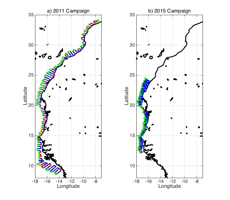
Figure 1: Survey design carried out off northwest Africa during acoustic annual assessment surveys at sea in 2011 and 2015 (Research Vessel Dr. Fridtjof Nansen). The classes appear in the following order: in green, the part of the echogram with no bottom; in blue, the part of the echogram requiring only a weak correction from the expert; in red, the pings requiring a strong correction from the fisheries acoustic experts. . (For interpretation of the references to color in this figure legend, the reader is referred to the web version of this article.)

Table 1: Summary of the variables present in each 2011 and 2015 sea survey datasets dimensions and associated labels. The main variables used to process the data and furthermore to set up the machine learning model are described. $S_{v}$ means volume backscattering strength (in dB).

	Depth	Echogram	Bottom	Clear Bottom
2015 dataset dimensions: [Nb. rows, Nb. columns]	[2567, 1]	[2567, 2 000 000]	[1, 2 000 000]	[1, 2 000 000]
2011 dataset dimensions: [Nb rows, Nb columns]	[2581, 1]	[2581, 2 661 003]	[1, 2 661 003]	[1, 2 661 003]
Units	Meter (m)	$S_{v}$ in dB	Meter (m)	Meter (m)
Horizontal/vertical vectors	Vertical vector: every cell correspond to a value in meter	Matrix: every column is a given ping, and every row a value in dB corresponding to a depth	Horizontal vector: every column gives the bottom depth found by the automatic procedure	Horizontal vector: every column gives the bottom depth corrected by the expert

2 Materials and Methods

In section 2.1 we provide an exhaustive description of the crude dataset collection, formatting, labeling method, and the subdivision in training, validation, and test datasets. Computing means and associated limitations on the size of the processed dataset are also described here. In section 2.2 we present the methodology for learning algorithms comparison, for training dataset optimization and the training settings.

2.1 Data Processing

2.1.1 Description of the crude dataset

Acoustic data came from an international collaboration of northwest African fishery research centers, which gathered their data at the subregional level. The data consist of two datasets corresponding to two campaigns from the Nansen project (Fisheries Research Vessel Dr. Fridtjof Nansen) that took place in 2011 and 2015 off northwest Africa (Fig 1) (e.g., Sarré et al. 2018). Here, each acoustic pulse is called a ping, and we call the matrix obtained from gathering the backscattered signals of a sequence of pings the echogram. These echograms usually come from preprocessed acoustic surveys at sea (Fig 1). The data preprocessing was done using the Matecho software (Perrot et al. 2018). The backscattered signal from the upper 500 m of the water column was extracted, and the echo at each depth was interpolated on a regular grid with a vertical resolution of 20 cm. Still, during preprocessing, the ocean depth for each ping was estimated by an automatic algorithm that searched for the maximum gradient of the acoustic signal, usually corresponding to the acoustic signal at the bottom. Then in post-processing, the echogram and the automatic bottom line detection were visualized by an expert who manually performed the correction of the bottom line.

Data were acquired with an echosounder fixed to the hull of the vessel. The vessel sent out acoustic wave pulses of four distinct frequencies in the water at a pulse length of 1 ms. In this study, we used the 38 kHz frequency as it is a common frequency used in fisheries acoustics and is not limited over the continental shelf (500–600 m maximum depth). Table 1 gives a summary of the variables present in each dataset used. The crude echogram presents some irregularities due to the onboard recording settings. Typical errors of the automatic procedure for bottom line detection are shown in Fig. 2a., and it can be seen that the expert (red line) roughly cut this part to avoid including the bottom signal in the echo-integration.

In particular, NaN (not a number) values were usually present between 500 m (the maximum recording depth in this case study) and $\sim$20–30 m below the predicted bottom. This is because, during data collection at sea, the echo sounder operator(s) set the maximum depth to limit data acquisition to the water column. Nevertheless, in some cases, real values were still attributed to much greater depths under the actual bottom (Fig 2). Furthermore, these irregularities were distributed differently between the 2011 and 2015 datasets (Fig 2) as they were dependent on the survey configuration at sea vs. the local depth surveyed. These irregularities, common in fisheries acoustics sea surveys, typically challenge traditional ML approaches. Indeed, to deal with such differences in the dataset’s noise the modeler is often required to build complex pipelines for feature extraction. The rationale behind the use of DL is to learn in an end-to-end fashion, with as few preprocessing operations as possible.

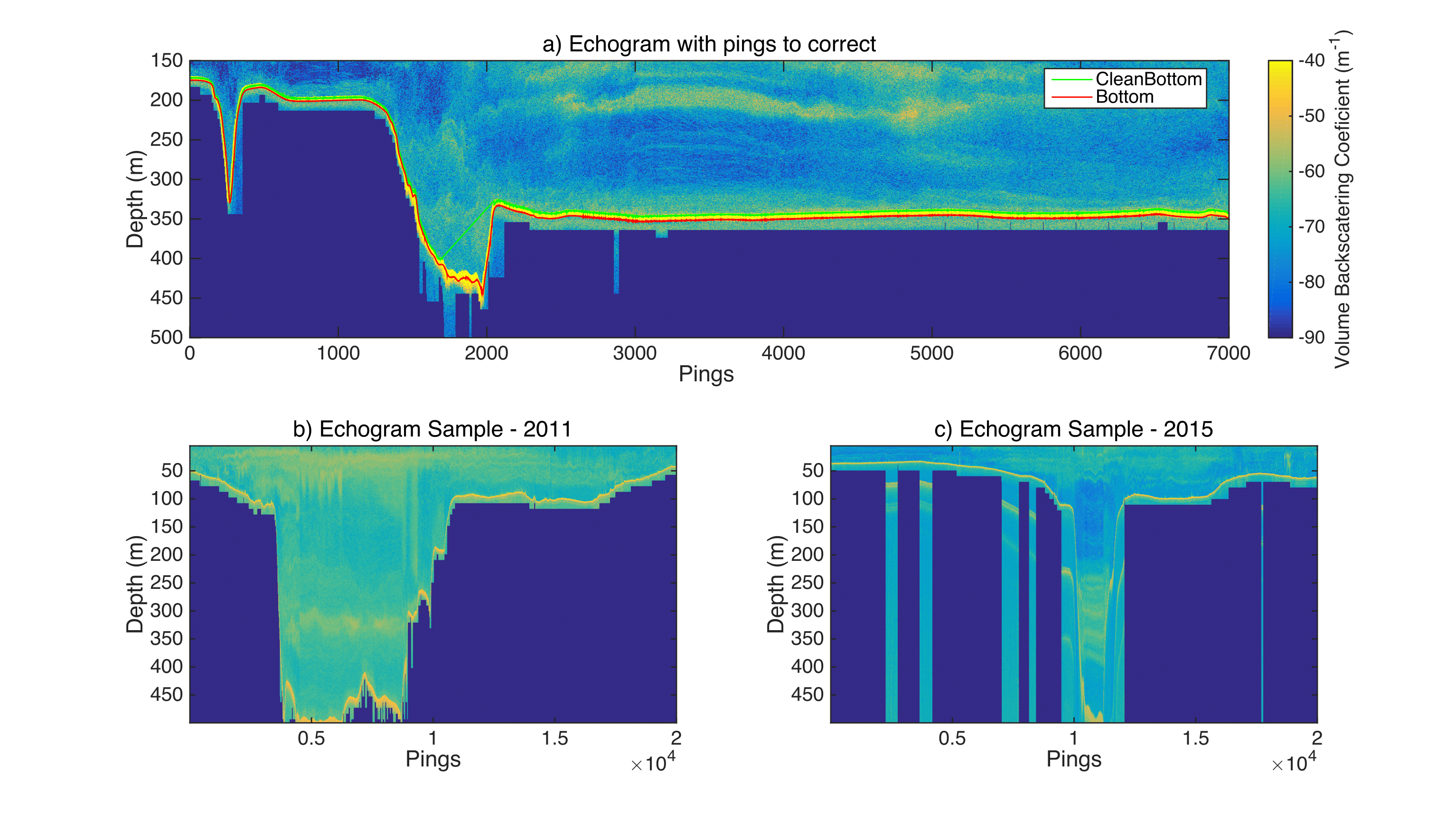
Figure 2: Echogram extracted from the acoustic sea survey used in the study. (a) An example in which the automatic procedure for bottom detection (green line) has failed around ping 2000. (b) Random samples from the 2011 and (c) 2015 echograms, with the same ping size and cell number; showing differences with respect to the settings for NaNs (“not a number”, strong blue color) below the bottom. Unit: see color bar in panel (a). . (For interpretation of the references to color in this figure legend, the reader is referred to the web version of this article.)

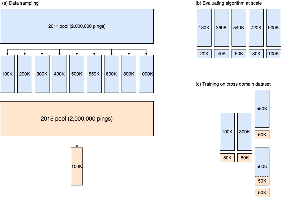
Figure 3: Sampling methodology. Subfigure (a) summarizes the data sampling strategy. Subfigure (b) shows the training and test set sizes as described in experiment 2.2.1. Subfigure (c) shows the setting proposed for experiment 2.2.3. The blue color corresponds to data from 2011 and the orange color corresponds to data from 2015. In (b) and (c), the longer boxes correspond to the training dataset. In (b) the small boxes are used as a test set and in (c) as a validation set.

Table 2: 2011 and 2015 sea survey dataset after removing pings without bottom and after removing the first cells of each dataset so that they share the same number of rows.

	Echogram	Label
2015 formatted dataset: [No rows, No columns]	[2550, 1 851 950]	[1, 1 851 950]
2011 formatted dataset: [No rows, No columns]	[2550, 2 321 967]	[1, 2 321 967]

2.1.2 Formatting the dataset

Three transformations were applied to extract a standardized format and minimalist training dataset from the crude one. We reduced the size of the training dataset to reduce learning and upload times on remote calculation servers.

The first transformation was carried out to get the same number of rows for our datasets, which initially varied slightly (Table 1). To do that, we removed the first 31 rows from the entire 2011 echogram ($\sim$ 6 meters), as well as the first 17 rows of the 2015 echogram ($\sim$ 3.3 meters). This was required because frequently there were strong signals in the first rows that subsequently disturbed the learning process. Such a transformation was necessary to allow the same neural networks to be trained and applied to the two dataset subsamples. Finally, we were left with 2550 rows in each of the preprocessed datasets.

The second transformation was aimed at reducing the size of the dataset by removing pings for which no learning could be extracted, to distinguish between bottom qualities, i.e., when pings in the echogram did not hit the bottom. This occurred when the vessel was located in areas deeper than 500 m because only the first 500 m were recorded during the sea campaign. These pings were removed using a threshold-based filter. We discriminated between the echograms with and without a bottom, based on the presence or absence of strong backscattering (> $-$32 dB), considered as a bottom signature. Finally, as we needed every ping to have the same dimensions for further calculation, and numerical algorithms could not process NaN values, we replaced all of the NaN values by -200 dB, a value that corresponds to the weakest recorded values in the echograms (-199 dB for 2011 and -198 dB for 2015). This operation can be seen as replacing non-recorded values by noise. Indeed, values below $\sim-$90 dB are never (or seldom) considered in fisheries acoustics analysis. Thus, NaN values were treated as area-located under the bottom and not reached by the acoustic signal. The sizes of the 2011 and 2015 formatted datasets are summarized in Table 2. Finally, both datasets were standardized before training.

2.1.3 Data labeling

We followed a generic ML methodology (Goodfellow et al. 2016). The goal of the procedure is to classify the data (here, acoustic pings) into two classes before the intervention of the expert to rationalize their work when correcting the crude echogram. The first class gathers the pings on which the automatic procedure usually performed well, thus needing less attention from the expert. The second class regroups the pings for which the expert usually needed to correct the automatic bottom prediction. We labeled each remaining ping (after formatting; see the previous section) as belonging to one of these two classes according to the distance between the expert correction (variable "CleanBottom", Table 1) and the initially predicted bottom depth (variable “Bottom,” Table 1). Thus, if |CleanBottom - Bottom| < 3.31, pings were labeled “weak correction,” i.e., no or weak expert correction needed, while if |CleanBottom - Bottom| >= 3.31, pings were labeled “strong correction,” i.e., major expert correction needed. Examples of these two classes are shown in Fig 2. The threshold value of 3.31 was chosen by comparing the accuracy obtained after one epoch of training for different threshold values ranging from 1.00 to 5.00 with a step of 0.01, and we selected the threshold that gave us the best classification accuracy. The distribution of those classes varied significantly from 2011 to 2015. Indeed, the class of strong correction accounted for 13% of the pings in 2011, whereas it accounted for only 1% in 2015. As can be seen in Fig 1, there is no clear pattern from the pings to correct. Hence, we expect to use ML methods to automate the finding of the ping, with a high likelihood of requiring a strong correction.

2.1.4 Sampling methodology

Here we describe datasets that were used to (1) optimize hyperparameters, (2) compare learning algorithms performances, and (3) train the best-identified learning algorithm with a mixed dataset. To begin with, the first 2,000,000 pings of each campaign were selected to constitute the pool of data. 2,000,000 was the maximum we can fit into memory. In the following, to ease the notation every 1000 pings are going to be treated as 1K pings. For the Bayesian optimization, we used a dataset of 100K pings randomly extracted from the complete 2011 pool dataset (Fig 3a). For comparing learning algorithms performances, datasets with successive sizes of 200K, 400K, 600K, 800K, and 1000K pings were also extracted from the 2011 pool dataset (respectively 2.0, 4, 6.0, 8.0, and 10.0 Go). The largest dataset used for training was made of 1000K pings because it was tedious to upload large datasets on GPU clusters online. Furthermore, to compare different learning algorithms, each of these datasets was split into 90% of the pings for the training set and 10% for the test set (Fig 3b). To evaluate the effect of cross-domain training on the best-identified algorithm, 100K, 300K, 500K, and 550K pings were sampled from the 2011 pool dataset for training along with 100K pings following each other from the 2015 pool. Those 100K pings were further randomly divided into two datasets of 50K pings, one that would serve as a validation dataset and one that would serve for cross-training (Fig 3c).

2.1.5 Computing Means and Limitations

Formatting of the dataset and the labeling operations were performed on a personal computer. For training purposes, we uploaded the dataset on a cloud platform to perform further calculations with graphical processing units (GPUs). However, the local Internet connection speed and stability limited the size of the dataset that could be uploaded. Also, the size of the unzipped 2011 preprocessed echogram was 22.81 Gigabytes, which scarcely fitted into random access memory (RAM). For training algorithms, a maximum of 1000K pings has been used to allow the dataset to be uploaded.

2.2 Experimental set up

2.2.1 Methods for Comparing learning algorithms performances

The first experiment was to compare the ability of different algorithms to learn from echosounder datasets at different scales. The compared algorithms suggested in the literature, were Random Forests (RF), Support Vector Machines (SVM), Feed-Forward Neural Networks (FFNN) and Convolutional Neural Networks (CNN) (LeCun and Bengio 1995; Niu et al. 2017 ; Ferguson et al. 2018).

A principled approach to compare machine-learning algorithms is to find their respective hyperparameters following a single optimization method. Here we used Bayesian Optimization (BO) as opposed to grid search and random search, as it has been shown that Bayesian optimization finds better hyperparameters significantly faster than random search which is superior to grid search (Snoek et al. 2012). Moreover, BO surpasses a human expert at selecting hyperparameters on the competitive CIFAR-10 dataset frequently used to benchmark computer vision algorithms (Snoek et al. 2012).

In this study, we used the open source python Library GyOpt (SheffieldML, 2020) for BO, with expected improvement as acquisition function and Gaussian Processes to model the surrogate function with the acquisition parameter equal to 0.1. For each algorithm, we fixed the range of variation for a set of hyperparameters. For RF the most sensitive hyperparameters according to (Niu et al. 2017) are the number of decision trees (range [10,1000]) and the minimum samples per leaf (range [20,50]). Concerning SVM we chose a linear kernel as the number of features is important (2500) (Hsu et al. 2003) and we optimize only the hyperparameter C (range [10, 1000]). The FFNN was chosen to have 3 hidden layers (ranging respectively [5,600], [5, 320] and [5,120] neurons) and with dropout (Srivastava et al. 2014) for the last hidden layer (ranging [0,1]. Every hidden layer used SELU (Klambauer et al. 2017) as an activation function. Finally, the CNN hyperparameters were three convolutional layers (with kernels ranging in [5, 60]) featuring batch normalization (Ioffe and Szegedy, 2015), followed by three hidden layers (with the same range as the FFNN), and with only dropout applied at the last hidden layer (range [0,1]). For BO, each learning algorithm was trained with a subset of 100,000 pings from the 2001 dataset, (Fig 3). The procedure was repeated for 50 iterations. At each iteration, the hyperparameters are tuned and the best validation accuracy is recorded. The maximum number of iterations was set to 50, but BO can stop before if hyperparameters converge.

Once the set of hyperparameters that maximize learning were found for each algorithm, we trained each algorithm on 5 datasets of sizes: 200K pings, 400K pings, 600K pings, 800K pings and 1,000K pings ( 2.0, 4, 6.0, 8.0 and 10.0 Go, respectively) to evaluate their respective ability to scale to big data. Also, the experiment was repeated 5 times to evaluate parameters‘ sensitivity to the learning process. Furthermore, SVM, FFNN, and CNN were trained for 100 epochs each. The test accuracy of both the CNN and the FFNN were obtained using Monte Carlo Dropout (Gal et al. 2015). In other words, their performance was assessed on the test set 50 times and the mean value was recorded. Monte Carlo Dropout allows neural networks to express uncertainty for their prediction due to the dropout factor at the end of the network. It has been proven to yield better results than standard test evaluation (standalone test run) (Gal et al. 2015). The SVM and RF were trained with Scikit-learn (Pedregosa et al. 2011). The framework allowed us to use multiprocessing, and the computation was distributed on 6 processors. SVM was trained with stochastic gradient descent. FFNN and CNN were trained with TensorFlow (Abadi et al. 2016). Parameters were updated after each epoch using the Adam optimization procedure with default parameters (Kingma et al. 2014) and binary cross-entropy as cost function.

2.2.2 Comparing simple and cross domain training

The requirement to explore the effect of learning on a cross-domain dataset was to display the normal learning curve when we scaled the size of the training set and compare it with a learning curve made with a cross-domain dataset. We compared the effect of mixing during training on the dataset coming from each pool of data (2011 and 2015). To this end, the subsample of 100,000 pings from 2015 was randomly divided into two datasets of 50,000 pings; one for the validation set, and the other that would be used to mix with data from 2011 (see Fig 3 and § hereafter).

Firstly, we successively trained on two datasets of sizes: 100,000 and 300,000 pings to get a baseline learning curve, denoted respectively as ST-100K and ST-300K (simple training 100K pings and simple training 300K pings). Secondly, to evaluate the impact of mixing two datasets with different label distribution and different noise structure we trained on two datasets of size 550,000 pings described as follows: (1) 550,000 pings randomly sampled from the 2011 pool dataset only (hereafter referred as ST-550) and (2) a mix of 500,000 pings randomly sampled from the 2011 pool dataset and 50,000 pings randomly selected from the 100,000 subsample ping 2015 datasets (hereafter referred as CDT-550K). The rationale behind the second approach was to avoid overlearning from the irregularities and data distributions specific to the 2011 dataset, and to assess the effect of mixing during training. Finally, the generalization performance of each model was evaluated locally by testing the classification accuracy of the models trained in each setting (ST-100K, ST-300K, ST-550K, and CDT-550K) on two test sets: on one hand the remaining unseen part of the 2011 dataset, on the other hand, the unseen part of the 2015 dataset.

3 Results

3.1 Comparing learning algorithms’ performances

The best validation accuracy obtained for a set of hyperparameters were obtained in less than 10 iterations for SVM and in about 22 iterations for RF. This is sound, indeed RF has two hyperparameters and SVM only one. On the other hand, FFNN and CNN improved but were not settled even after 50 iterations (Fig 4). The final set of hyperparameters for each learning algorithm is displayed in Table IV. Learning algorithms’ performances were then compared when trained with increasing size of datasets. Support Vector Machines (SVM) did not increase its performance when augmenting dataset size; surprisingly it seems to even worsen (Fig 5a). Feed-Forward Neural Network (FFNN) exhibits the greater variability, for every size of the training set the worst value is almost approximately the same and is the result of sticking on a local minimum as the training loss did stagnate during training. Note that in the experiment on the 800K dataset the algorithm did not stick in any local minima (Fig 5a). As a result, the mean test accuracy suffered and explained the drop in performance for the last dataset. Random Forest (RF) displayed almost no variability and its performance benefited as a result of increasing dataset size.

Finally, Convolutional Neural Networks (CNN) got the highest mean test accuracy score right when training on 400K pings and more (Fig 5a). It is furthermore more stable to train as it displays less variability than FFNN while always having the best maximum test accuracy score. Except for Support Vector Machines (SVM), we observe that other learning algorithms scale well. With Feed-Forward Neural Network (FFNN) having the greatest variability in its gains. This is because FFNN is often stuck in local minima when learning starts. Random Forest (RF) also steadily increases its test accuracy when the dataset is scaled. The Convolutional Neural Networks (CNN), which never stuck in local minima, makes the highest gain.

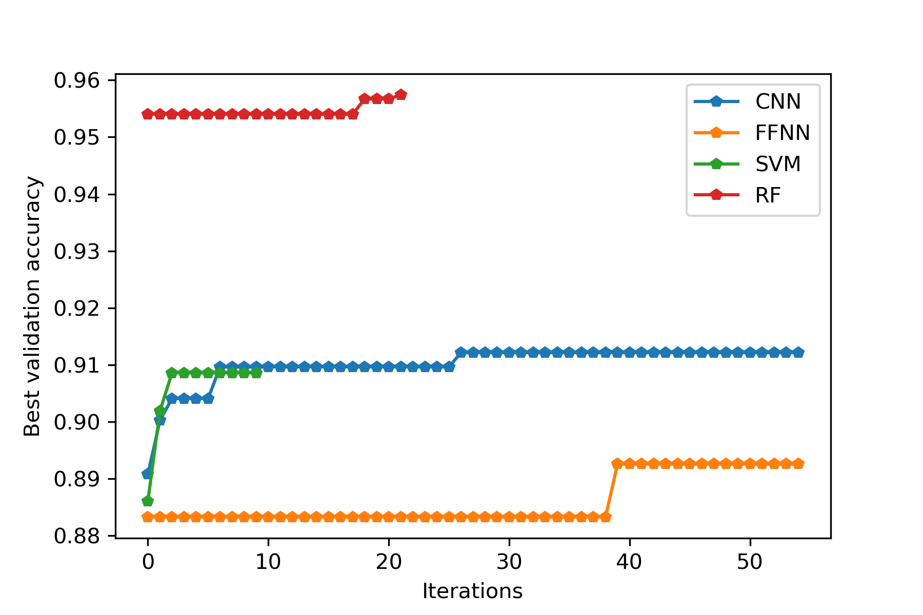
Figure 4: Illustration of the hyperparameters selection with Bayesian optimization procedure for Random Forests (RF), Support Vector Machines (SVM), Feed-Forward Neural Networks (FFNN) and Convolutional Neural Networks (CNN).

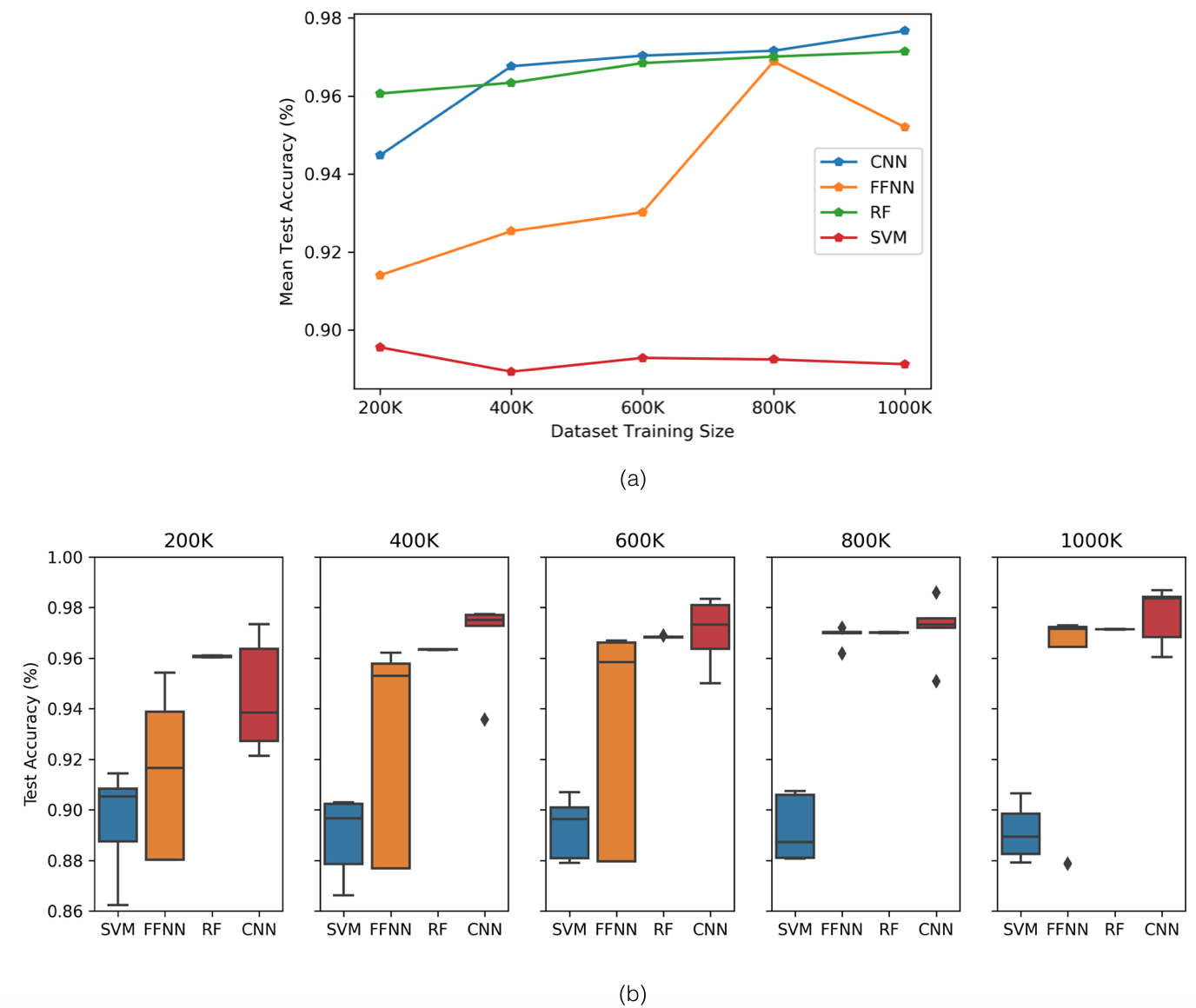
Figure 5: (a) Mean accuracy got for Random Forests (RF), Support Vector Machines (SVM), Feed-Forward Neural Networks (FFNN) and Convolutional Neural Networks (CNN) while varying the training dataset size from 200 000 to 1000 000 pings from the 2011 sea survey dataset. (b) Test accuracy summary statistics of each learning algorithm after 5 repetitions of the training process.

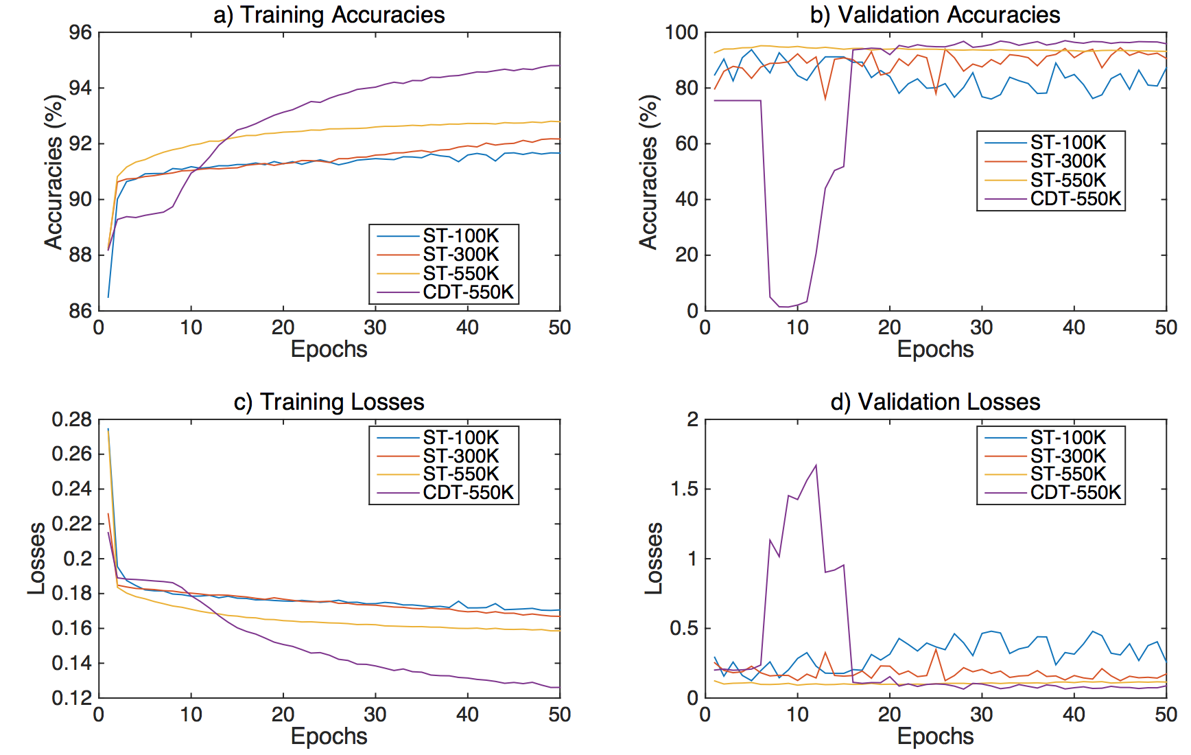
Figure 6: Performance at each iteration (epoch) of the model during training and validation on: simple training (ST) and cross-domain training (CDT) for 100,000, 300,000, and 550,000 pings. (a) training accuracy, (b) validation accuracy, (c) training losses and (d) validation losses. Validation accuracy and losses were obtained during training on a single unseen validation set from the 2015 sea survey dataset.

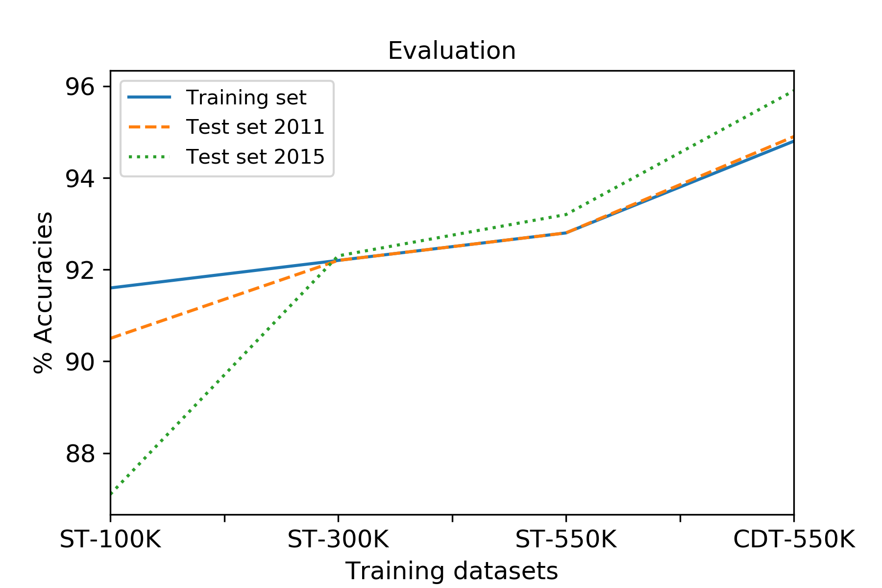
Figure 7: Evaluation of model accuracy on training dataset (solid line), 2011 test dataset (red circled line) and 2015 test dataset (green circled line) when increasing the training dataset size from 100,000 pings to 550,000 pings. See training datasets details in Section 2.1.4. . (For interpretation of the references to color in this figure legend, the reader is referred to the web version of this article.)

3.2 Improving generalization accuracy with a cross domain dataset

3.2.1 Learning evaluation on the training set

Training accuracies showed little difference when training on ST-100K and ST-300K; the latter displayed a slightly better evolution after epoch $\sim$25 (after 50 epochs respectively, 92%, and 92%; Fig 6a). With ST-550t, a net increase in training accuracy appeared after epoch 2 and reached 93% at the end of the training. When training on CDT-550K, the training accuracy increased slowly until epoch $\sim$8, but overtook the other training experiments after $\sim$15 epochs and finally reached 95% (Fig 6a). The training losses displayed similar (but symmetric) tendencies, reaching final losses of 0.17, 0.16, 0.15, and 0.12, respectively, for training with 100,000, 300,000, and 550,000 pings from the 2011 dataset, and 550,000 cross-domain pings (Fig 6c).

3.2.2 Learning evaluation on the validation set

In contrast to the continuous increase in training accuracy, in the case of simple training, the validation accuracy displayed a higher variance, with a flat tendency among epochs; the variability was smaller, however, for larger training datasets (Fig 6b). The average accuracy reached 87%, 91%, and 93%, respectively, for datasets ST-100K, ST-300K, and ST-550K at epoch 50. Note also that the validation accuracy obtained when training on ST-100K decreased over the epoch (Fig. 6b), which denoted a degree of over fitting. The effect of using a cross domain dataset for training was more evident from the validation performances. Indeed, the accuracy dropped to low values (0.1%) around epoch $\sim$10, but then rapidly reached higher values than those of the simple training set experiments after epoch 18, and then displayed a steady upward tendency, reaching a value of 96% at the end of the training process. Validation losses displayed the same change in variability among training experiments. The validation losses for simple training were 0.25, 0.17, and 0.11, and the final value for cross-domain training was 0.08 (Fig 6d). In summary, training on a cross-validation dataset yielded unstable performances during the first $\sim$15 epochs, however, after epoch 30, it outperformed training being done with simple datasets.

3.2.3 Generalization Performances

The generalization performance was evaluated by applying the CNN to predict ping classes on an unseen test set extracted either from the 2011 dataset or from the 2015 dataset (Fig 7). On the 2011 test set, the CNN trained with the ST-100K, ST-300K, ST-550K, and CDT-550K training sets correctly classified 90%, 92%, 93%, and 95% of the pings, respectively. On the 2015 test set, they correctly classified 87%, 92%, 93%, and 96% of the pings, respectively. The CNN

trained on only 100,000 pings from 2011 (ST-100K) over fitted, as its performance was better on the training data than on unseen data. The ST-300K training set led to a similar performance on all test sets. The ST-550K training set led to the same accuracy on the training set and on the 2011 test set. Unexpectedly, better accuracy was obtained when evaluating the 2015 test set than on the training and 2011 test sets. Finally, training on CDT-550K led to a leap in performance both on the training set and the 2011 test set but yielded an even better performance on the 2015 test set.

4 Discussion

Machine learning algorithms have been widely used in passive acoustics. Indeed, Shamir et al. (2014) introduced an automated method for target classification in bioacoustics. Yue et al. (2017) used support vector machines (SVM) and convolutional neural networks (CNN) for underwater target classification. Chi et al. (2019) used feed-forward neural networks (FFNN) for source ranging. Hu et al. (2018) applied CNN for underwater acoustic signal extraction. Many machine learning methods were employed for underwater source localization: Niu et al. (2017) compared SVM, Random Forests (RF), and FFNN, then, Ferguson et al. (2018) applied CNN for the same task and Wang et al. (2018) compared traditional match field processing (MFP) with FFNN and generalized regression neural networks. Finally, deep learning methods were also applied for underwater source localization: for instance, Huang et. al (2018) used FFNN in a shallow water environment, moreover, Niu et al. (2019) used deep CNN in the context of big data.

Yet, very few authors have applied deep learning algorithms on fisheries (active) acoustics data (see section 1.2; Williams 2016, Denos et al. 2017, Brautaset et al., 2020). A recent literature review of ML in acoustics is provided by (Bianco et al. 2019). One premise of deep learning is that it could allow us to treat crude data in an end to end fashion (LeCun et al. 2015).

Here we investigate ML methods on pre-processed echograms (see section 2.1.1). Using Matecho (Perrot et al. 2018) allows a full chain of processing methods to extract information and perform echo-integration on echosounder data following an international standard. The present study contributes to filling this gap and shows the potential of learning algorithms to serve as a useful tool for fisheries acoustics expert processing tasks. Below we first discuss the pipeline experimented here for bottom correction in fisheries acoustic dataset. Then, we identify the remaining challenge for this approach. We conclude on the main contribution of the paper and provide perspectives one the potential benefit of using ML in fisheries acoustics. Two patterns emerge from our experiments of applying ML to active acoustics data, with one of them fairly unexpected. Firstly, as expected in DL, increasing the size of the training data almost always leads to better performance on the training set but also on each test set. Secondly, using a cross-domain dataset for training leads to a leap in accuracy during training, validation, and at test time. This emphasizes the sensitivity of the generalization performance to the diversity of the training dataset.

Table 3: Accuracies evaluated by each model on the 2011 sea survey dataset and the 2015 dataset. It seems that adding a subset of the 2015 data within the training set helps the model to get a better performance on both test set. In bold the upper and lower accuracies.

Final accuracies (in %)	Training set	Test set — 2011	Test set — 2015
ST — 100k	92	91	87
ST — 300k	92	92	92
ST — 550k	93	93	93
CDT — 550k	95	95	96

Table 4: Hyperparameters search space and value found using a Python Bayesian optimization library (GyOpt).

Random forest
Hyperparameter	Search Space	Value
Number of tree range	[10, 10 000]	187
Min. samples leaf	[20, 50]	24

Support vector machines
Hyperparameter	Search Space	Value
Alpha	[0.0001, 0.1]	0.077

Feed-forward neural network
Hyperparameter	Search Space	Value
Number of neuron: fully connected layer 1	[5, 600]	75
Number of neuron: fully connected layer 2	[5, 320]	105
Number of neuron: fully connected layer 3	[5, 120]	95
Dropout rate: fully connected layer 3	[0, 1]	0.6

Convolutional neural network
Hyperparameter	Search Space	Value
Kernel 1	[5, 60]	5
Kernel 2	[5, 60]	59
Kernel 3	[5, 60]	19
Number of neuron: fully connected layer 1	[5, 600]	260
Number of neuron: fully connected layer 2	[5, 320]	319
Number of neuron: fully connected layer 3	[5, 120]	101
Dropout rate: fully connected layer 3	[0, 1]	0.9

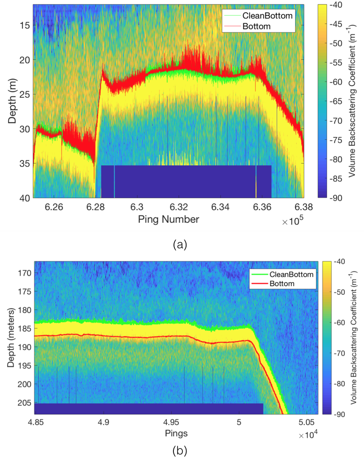
Figure 8: (a) Example of echogram in which automatic bottom detection (red line) failed due to presence of a planktonic layer directly above the sea floor (soft yellow). The green line is the bottom line after correction by the expert. (b) Example of echogram in which automatic bottom correction (red line) failed due to the transducer depth being moved down during the sea campaign showing a constant offset shift. . (For interpretation of the references to color in this figure legend, the reader is referred to the web version of this article.)

4.1 Learning algorithm comparison: why CNN stand out

SVM performed poorly, indeed this is because we used a linear kernel on a high dimensional problem, this was required to allow the SVM to learn on large datasets. Also as SVM do not allow to increase the number of parameters used to learn, it has a lower asymptote than the other models (Fig 5.a). While RF has the best accuracy when trained with a small dataset (200K), CNN proved to have better performance as soon as the datasets got bigger. Yet, RF is the second best option and followed the CNN closely even though the accuracy obtained with 1000K pings seemed to led the CNN accuracy to take off. Another interesting property of RF is that they exhibit almost no variability when compared among different training versions on the same dataset. This property allows the modeler to be sure that he got the best possible achievable result with a RF when training is achieved. The main advantage of neural networks, whether FFNN or CNN, is the ability they gave to the modeler to increase the number of the parameters to the learning problem. As a result, they are modular and can adapt to many kinds of problems. The main downside of FFNN was its variability from training to training. Indeed the reader can observe that the worst result obtained for each dataset is closely the same around 87% (Fig 5.b). At least for one run over the 5 we did, the FFNN achieved almost no learning. This can happen when the network is stuck in a local minimum and cannot get outside of it during training. In contrast, during training, the CNN has never fallen in a local minimum (Fig 5.b). This is because the convolutional layers compressed the original data in a lower-dimensional representation that is further passed to a fully connected neural network. As a result, the important features are summarised by the convolutional layers (Goodfellow et al. 2016, Lecun et al. 2015). And the optimization is made in a lower-dimensional space. Convolution has shown great promise for image understanding. The above comparison suggests that 1-dimensional convolution is the more adapted class of learning algorithm to process active echosounder data. Finally, CNN exhibits the best performance with training datasets of sizes 400K, up to 1000K. Niu et al. (2017) found comparable performance for each model: SVM, RF, and FFNN in underwater source localization framed as a classification problem. Our results differed from those of Niu et al. (2017) as we found a clear advantage of using neural networks and more specifically convolutional neural networks. This difference can be explained as they used a relatively small dataset for training (1,380 samples for training, 120 examples for testing), also their work was on simulated passive acoustic data. In contrast, our work was done on a real-world and bigger dataset (200,000 examples to 1,000,000 examples) of active acoustic data. Getting better results on bigger datasets with Deep Learning is discussed in Goodfellow et al. (2016) and Sun et al. (2017). Furthermore practical applications were found in underwater source localization by Niu et al. (2019) who used a 50 layers residual network to learn on tens of millions of training examples.

4.2 Cross domain training as a way to tackle imbalances and irregularities in datasets

The specific problem we tacked is the task of helping the expert to label a new dataset faster given past labeled data. An important assumption in ML is that the data we want to learn from as well as the future unseen data must come from the same distribution and be identically and independently distributed (Goodfellow et al. 2016). This is the first challenge that rose from the task at hand. This assumption does not hold in our case, as discussed in section 2.1.3 for the label distribution and as illustrated in Fig 2 for the noise distribution.

Methods that deal with unbalanced datasets exist (Shimodaira 2000; Crammer et al. 2008). However, these techniques need to know the distribution of the target dataset to correct imbalances during training. So, they do not apply in our case because the label distribution of a new dataset is unknown before the expert has labeled it. One could say that the expert could label a sample of the new dataset to get an estimation of the target label data distribution. There are approaches in the ML literature that deal exactly with this problem for instance semi-supervised learning (Chapelle et al. 2006) and active learning (Settles 2010). While these approaches could be envisioned in future work, they need to take into account the specificity of fisheries acoustics data. Indeed the labeling needs to occur for several pings following each other because the expert needs to get context from the ping in the same area to accurately label the bottom line. In a sense, the labeling process is not based on the review of individual pings but on the review of chunks of pings. This contrasts with traditional computer vision tasks, where the labeling of each image is independent of each other. In that sense, traditional active learning methods could be useful if applied to a chunk of data, or to individual pings with the goal to review every ping in a given neighborhood. Similarly, semi-supervised learning methods require training a model on a representative sample of labeled data, augmented with unlabeled data. The rationale is to use the structure of unlabeled data to learn useful features of the model that can be refined on the labeled dataset during training. This condition could be met if the expert selects a representative subset of ping and labels their neighborhood. In this paper, we took the simplest possible setting: to label a randomly selected chunk of 100,000 pings from the new dataset. As this is relatively easy to do in practice. Indeed, this chunk of data represents $\sim$5% of the total number of pings. Furthermore, we quantified if this chunk of pings could benefit the model at training time by monitoring its performance on a validation set made of this chunk of data (Fig 6). Finally, we evaluated the model trained in each setting, on two large test sets made of respectively all unseen ping from the 2011 and the 2015 pool. We observe that using a cross-domain dataset improves the performance on each test set (Fig 7), suggesting that novel features introduced by the new dataset add to the complexity of the cross-domain training set as opposed to the simple training set. Indeed, even the accuracy on the training set improved. The optimization procedure during training seems to be less stable in the first few epochs, this is probably due to a different path taken by the algorithm when updating its weights.

Also, note that while the current system got 96% accuracy (Table III) on the 2015 test set, its performance could be enhanced by training on a larger database composed of diverse sea surveys. Indeed, we have shown that training with an increasingly bigger training set size leads to better results with local test sets (Fig 3; Fig 5). In addition, we have shown the potential of mixing datasets (Fig 7). This is in line with the results of Sun et al. (2017), more data is always welcome for deep learning models.

4.3 Challenges of Machine Learning methods with Fisheries Acoustics Data

Although the 2011 and 2015 datasets were collected in the same area, i.e., the northwest African continental shelf, using the same vessel, there was a great divergence in the error distribution of the initial bottom line estimation, which was subsequently corrected by experts. There were also irregularities in the noise distribution of the data between the 2011 and 2015 echograms (Fig 2). Indeed, it is often the case that datasets collected from different sea surveys present different attributes even if they were collected in the same geographical area. This may be due, for example, to different weather conditions encountered during the two sea surveys (wind and sea agitation). Indeed, the bottom reflection signal can be altered by air bubbles (generated by wave breaking), as well as by the ship’s roll and pitch. Bottom line correction also depends on the biological resources targeted. For example, the expert corrects the bottom line more carefully when the echointegration concerns resources close to the bottom line, as opposed to pelagic species occurring in the water column, since a precise bottom estimation is less crucial for the latter. As a result, even during post-processing by the expert for bottom correction, we can have part of the echogram being corrected with less accuracy. Errors can be caused by the detection of biological resources in contact with the bottom (e.g., planktonic layer or fish school) (Fig 8.a) or a change in the transducer depth settings by an operator on board the vessel (Fig 8.b). Also, different settings of the echosounder during the data collection may yield a different noise distribution. These differences between different datasets may explain the surprising result of better performances on the 2011 test set than on the training set in the case CDT-550K (Fig 7). However, it does not clearly explain why the CNN trained with a CDT-550K performed better at classifying the 2015 test set than classifying the 2011 test set (Fig 5).

One hypothesis that may explain this phenomenon is that the 2011 dataset benefited from a much greater degree of human correction than the 2015 dataset. Indeed, in proportion, more pings have been corrected in the 2011 dataset than in the 2015 dataset as discussed in section 2.1.3. Consequently, we learned on a dataset with a higher likelihood of including bad labeling, in other words, we trained on a dataset harder to learn. Yet, as stated in his survey of DL methods in remote sensing (Ball et al. 2017), the question of how the DL algorithm ingests non heterogeneous data sources is still open. Our interpretation, though, is that since the loss function is not convex, the minimization problem admits multiple local minima, thus ingesting heterogeneous data may influence the weights update trajectory during training. And a more diverse training set leads to better minima.

4.4 Limitations due to the labeling process

The other obvious limitation is relative to the data labeling process. We discriminated our data based on a threshold that we found when computing the numerical difference between the bottom line calculated by the onboard procedure and the expert post-processing corrected bottom line (referred to as “clean bottom”). However, in some cases this difference was not due to echogram noise that could be detected by an algorithm (as shown in Fig 8.a). For example it could occur if the transducer was moved up or down (on the onboard setting or concretely) during the sea campaign, as a result the bottom given by the procedure is under the real bottom, even if the bottom line appears from the echogram structure (Fig 8.b). The issue is that such echograms are labeled as needing expert correction while nothing should have generated an error in bottom localization, since the error comes from an external reason (here a change of the transducer depth settings during the sea campaign). Thus, this kind of labeling in the training dataset limits the quality of the learning process.

Finally, we have reported several factors that could influence the quality of the training dataset and limit the classification performance that can be achieved with a trained algorithm on different dataset. Indeed, the occurrence of cases where the bottom correction errors do not come from the echogram structure alone might prevent an optimal classification by the trained CNN.

4.5 Perspective and Future Works

We see two main dimensions in which this work can be extended: (1) by improving the efficiency and the quality of the methodology, (2) by working toward an operational tool for the fisheries acoustics community. A more careful annotation of the data would yield better results in terms of accuracy and interpretability of how the model learns. In this respect, changing the data labeling procedure can bring significant improvements. For example, instead of using a criterion based on the difference in the distance between the bottom and the clean bottom, one could compare the amount of energy in the echogram (in mean volume backscattering strength (Sv in dB)) at the respective depths of the bottom and the clean bottom. In the same way, it might be interesting to use a depth offset for a given time interval, with the rationale that the bottom value cannot jump, given two consecutive pings, except when there is a particular bottom relief. Also, a multi-criteria procedure for labeling each ping could be considered if the computing power available for training allows it. Future studies will need to experiment with more datasets from diverse geographic areas to further study the benefits of generalization from learning with multiple datasets. In particular, this would allow further study on the effects of data irregularities and distribution differences in the learning process. A good starting point toward that goal would be to use active learning or semi-supervised learning methodologies (Chapelle et al. 2006; Settles 2010).

We advocate that working upfront on a unified data collection procedure would certainly reduce errors due to data irregularities and also reduce the variability coming from different experts concerning the labeling process. Using machine learning to standardize the labeling process across geographical regions would be useful to enable more meaningful application for the downstream modeling task of fish density estimation. A step toward that direction would be to create a common pool of labeled fisheries acoustics data and to train a deep convolutional neural network on it. This would result in the best performance achievable because as we have shown, the quantity and the diversity of the dataset play a key role to improve the performance of DL models. The trained model could then be used to standardize the labeling of new sea surveys collected globally. One of the benefits of having a uniform labeling process across geographical regions is to allow for comparative studies of new computational methods in fisheries acoustics.

5 Conclusion

The goal of this work was to develop a system designed to help a human expert to correct the bottom line from echogram data. Our main contribution to the study of fisheries acoustics has been to establish that CNN are able to extract useful features from different underwater active acoustic data sources. To address inherent imbalances in data distribution, as well as irregularities, a good practice is to learn with a cross-domain training set. The model trained can be used to help the fisheries acoustics expert to find pings that are likely to require correction on the bottom line with a high accuracy (>95%). However, our results suggest that much better classification accuracy can be reached using larger and more diverse datasets for training; such an approach could easily be implemented using dedicated GPUs. Finally, this work demonstrates the potential of CNN to learn features from fisheries acoustics data. This suggests that DL could be used furthermore to standardize the labeling process across regions and open the road to interesting areas of research based on large historical acoustic datasets in which other objects such as fish schools have been labeled (e.g., Scalabrin and Massé 1993; MacLennan et. al. 2004; Trygonis et al. 2016) to better discriminate between fish schools and sound scattering layers (Diogoul et al. 2020). Particularly demersal fish schools near the bottom as well as seabed echoes.

6 Acknowledgments

We are grateful to the AWA Project (“Ecosystem Approach to the management of fisheries and marine environment (EAMME) in West African waters”) funded by the German Federal Ministry of Education and Research (BMBF) and the French Research Institute for Development (IRD) (Grant 01DG12073E) implemented by the Sub-Regional Fisheries Commission (SRFC), the Preface Project funded by the European Commission’s Seventh Framework Program (2007–2013) under Grant Agreement No. 603521, EU TriAtlas project (Grant Agreement No. 817578) and the FAO/Nansen Project for data collection. We are grateful to Adrien Berne (IRD, France) who performed the manual clean-bottom corrections for both surveys, to Dr Jens-Otto Krakstad of the Norwegian Institute of Marine Research (IMR) who led the surveys at sea off northwest Africa, and to Gildas Roudaut and Jérémie Habasque (IRD, France) for their early interest in this approach and expertise in fisheries acoustics labeling. We are also grateful to Théophile Bayet (IRD) for constructive discussions and comments.

References

- [Abadi et al., 2016] Abadi, M., Agarwal, A., Barham, P., Brevdo, E., Chen, Z., Citro, C., Corrado, G. S., Davis, A., Dean, J., and Devin, M. (2016). Tensorflow: Large-scale machine learning on heterogeneous distributed systems. arXiv preprint arXiv:1603.04467.
- [Ball et al., 2017] Ball, J. E., Anderson, D. T., and Chan, C. S. (2017). Comprehensive survey of deep learning in remote sensing: theories, tools, and challenges for the community. Journal of Applied Remote Sensing, 11(4):042609.
- [Bartholomä, 2006] Bartholomä, A. (2006). Acoustic bottom detection and seabed classification in the German Bight, southern North Sea. Geo-Marine Letters, 26(3):177.
- [Bianco et al., 2019] Bianco, M. J., Gerstoft, P., Traer, J., Ozanich, E., Roch, M. A., Gannot, S., and Deledalle, C.-A. (2019). Machine learning in acoustics: Theory and applications. The Journal of the Acoustical Society of America, 146(5):3590–3628. Publisher: Acoustical Society of America.
- [Brautaset et al., 2020] Brautaset, O., Waldeland, A. U., Johnsen, E., Malde, K., Eikvil, L., Salberg, A.-B., and Handegard, N. O. (2020). Acoustic classification in multifrequency echosounder data using deep convolutional neural networks. ICES Journal of Marine Science.
- [Brehmer, 2006] Brehmer, P. (2006). Fisheries Acoustics: Theory and Practice, 2nd edn. Fish and Fisheries, 7.
- [Brehmer et al., 2019] Brehmer, P., Sancho, G., Trygonis, V., Itano, D., Dalen, J., Fuchs, A., Faraj, A., and Taquet, M. (2019). Towards an autonomous pelagic observatory: experiences from monitoring fish communities around drifting FADs. Thalassas: An International Journal of Marine Sciences, 35(1):177–189. Publisher: Springer.
- [Brehmer et al., 2006] Brehmer, P., Vercelli, C., Gerlotto, F., Sanguinède, F., Pichot, Y., Guennégan, Y., and Buestel, D. (2006). Multibeam sonar detection of suspended mussel culture grounds in the open sea: Direct observation methods for management purposes. Aquaculture, 252(2-4):234–241.
- [Chapelle et al., 2010] Chapelle, O., Schlkopf, B., and Zien, A. (2010). Semi-Supervised Learning. The MIT Press, 1st edition.
- [Chi et al., 2019] Chi, J., Li, X., Wang, H., Gao, D., and Gerstoft, P. (2019). Sound source ranging using a feed-forward neural network trained with fitting-based early stopping. The Journal of the Acoustical Society of America, 146(3):EL258–EL264. Publisher: Acoustical Society of America.
- [Chollet and others, 2015] Chollet, F. and others (2015). Keras.
- [Crammer et al., 2008] Crammer, K., Kearns, M., and Wortman, J. (2008). Learning from multiple sources. Journal of Machine Learning Research, 9(Aug):1757–1774.
- [Deng et al., 2009] Deng, J., Dong, W., Socher, R., Li, L.-J., Li, K., and Fei-Fei, L. (2009). Imagenet: A large-scale hierarchical image database. In 2009 IEEE conference on computer vision and pattern recognition, pages 248–255. Ieee.
- [Denos et al., 2017] Denos, K., Ravaut, M., Fagette, A., and Lim, H. (2017). Deep learning applied to underwater mine warfare. In OCEANS 2017 - Aberdeen, pages 1–7.
- [Diogoul et al., 2020] Diogoul, N., Brehmer, P., Perrot, Y., Tiedemann, M., El Ayoubi, S., Mouget, A., Migayrou, C., Sadio, O., and Sarre, A. (2020). Fine-scale vertical structure of sound-scattering layers over an east border upwelling system and its relationship to pelagic habitat characteristics. Ocean Science, 16(1):65–81. Publisher: Copernicus Gesellschaft Mbh.
- [EK60, 2020] EK60, S. (2020). Reference manual.
- [Ferguson et al., 2018] Ferguson, E. L., Williams, S. B., and Jin, C. T. (2018). Sound source localization in a multipath environment using convolutional neural networks. In 2018 IEEE International Conference on Acoustics, Speech and Signal Processing (ICASSP), pages 2386–2390. IEEE.
- [Foote et al., 1991] Foote, K. G., Knudsen, H. P., Korneliussen, R. J., Nordbo/, P. E., and Ro/ang, K. (1991). Postprocessing system for echo sounder data. The Journal of the Acoustical Society of America, 90(1):37–47.
- [Gal and Ghahramani, 2015] Gal, Y. and Ghahramani, Z. (2015). Bayesian convolutional neural networks with Bernoulli approximate variational inference. arXiv preprint arXiv:1506.02158.
- [Goodfellow et al., 2016] Goodfellow, I., Bengio, Y., Courville, A., and Bengio, Y. (2016). Deep learning, volume 1. MIT press Cambridge.
- [Griffin et al., 2007] Griffin, G., Holub, A., and Perona, P. (2007). Caltech-256 object category dataset. Publisher: California Institute of Technology.
- [Guillard et al., 2010] Guillard, J., Balay, P., Colon, M., and Brehmer, P. (2010). Survey boat effect on YOY fish schools in a pre-alpine lake: evidence from multibeam sonar and split-beam echosounder data. Ecology of freshwater fish, 19(3):373–380.
- [Hsu et al., 2003] Hsu, C.-W., Chang, C.-C., and Lin, C.-J. (2003). A practical guide to support vector classification. Taipei.
- [Hu et al., 2018] Hu, G., Wang, K., Peng, Y., Qiu, M., Shi, J., and Liu, L. (2018). Deep Learning Methods for Underwater Target Feature Extraction and Recognition. Computational intelligence and neuroscience, 2018.
- [Huang et al., 2018] Huang, Z., Xu, J., Gong, Z., Wang, H., and Yan, Y. (2018). Source localization using deep neural networks in a shallow water environment. The Journal of the Acoustical Society of America, 143(5):2922–2932. Publisher: Acoustical Society of America.
- [Ioffe and Szegedy, 2015] Ioffe, S. and Szegedy, C. (2015). Batch normalization: Accelerating deep network training by reducing internal covariate shift. arXiv preprint arXiv:1502.03167.
- [Kingma and Ba, 2014] Kingma, D. P. and Ba, J. (2014). Adam: A method for stochastic optimization. arXiv preprint arXiv:1412.6980.
- [Klambauer et al., 2017] Klambauer, G., Unterthiner, T., Mayr, A., and Hochreiter, S. (2017). Self-normalizing neural networks. In Advances in Neural Information Processing Systems, pages 971–980.
- [Korneliussen, 2004] Korneliussen, R. J. (2004). The Bergen echo integrator post-processing system, with focus on recent improvements. Fisheries Research, 68(1-3):159–169. Publisher: Elsevier.
- [LeCun and Bengio, 1995] LeCun, Y. and Bengio, Y. (1995). Convolutional networks for images, speech, and time series. The handbook of brain theory and neural networks, 3361(10):1995.
- [LeCun et al., 2015] LeCun, Y., Bengio, Y., and Hinton, G. (2015). Deep learning. nature, 521(7553):436.
- [MacLennan, 1986] MacLennan, D. N. (1986). Time varied gain functions for pulsed sonars. Journal of Sound and Vibration, 110(3):511–522.
- [MacLennan et al., 2004] MacLennan, D. N., Copland, P. J., Armstrong, E., and Simmonds, E. J. (2004). Experiments on the discrimination of fish and seabed echoes. ICES Journal of Marine Science, 61(2):201–210.
- [McClatchie et al., 2000] McClatchie, S., Thorne, R. E., Grimes, P., and Hanchet, S. (2000). Ground truth and target identification for fisheries acoustics. Fisheries Research, 47(2-3):173–191. Publisher: Elsevier.
- [Niu et al., 2019] Niu, H., Gong, Z., Ozanich, E., Gerstoft, P., Wang, H., and Li, Z. (2019). Deep learning for ocean acoustic source localization using one sensor. arXiv preprint arXiv:1903.12319.
- [Niu et al., 2017] Niu, H., Reeves, E., and Gerstoft, P. (2017). Source localization in an ocean waveguide using supervised machine learning. The Journal of the Acoustical Society of America, 142(3):1176–1188. Publisher: Acoustical Society of America.
- [Ona and Mitson, 1996] Ona, E. and Mitson, R. B. (1996). Acoustic sampling and signal processing near the seabed: the deadzone revisited. ICES Journal of Marine Science, 53(4):677–690. Publisher: Oxford University Press.
- [Pedregosa et al., 2011] Pedregosa, F., Varoquaux, G., Gramfort, A., Michel, V., Thirion, B., Grisel, O., Blondel, M., Prettenhofer, P., Weiss, R., and Dubourg, V. (2011). Scikit-learn: Machine learning in Python. the Journal of machine Learning research, 12:2825–2830. Publisher: JMLR. org.
- [Perrot et al., 2018] Perrot, Y., Brehmer, P., Habasque, J., Roudaut, G., Behagle, N., Sarré, A., and Lebourges-Dhaussy, A. (2018). Matecho: An Open-Source Tool for Processing Fisheries Acoustics Data. Acoustics Australia, pages 1–8.
- [Raykar et al., 2010] Raykar, V. C., Yu, S., Zhao, L. H., Valadez, G. H., Florin, C., Bogoni, L., and Moy, L. (2010). Learning from crowds. Journal of Machine Learning Research, 11(Apr):1297–1322.
- [Sarré et al., 2018] Sarré, A., Krakstad, J.-O., Brehmer, P., and Mbye, E. M. (2018). Spatial distribution of main clupeid species in relation to acoustic assessment surveys in the continental shelves of Senegal and The Gambia. Aquatic Living Resources, 31:9.
- [Scalabrin and Massé, 1993] Scalabrin, C. and Massé, J. (1993). Acoustic detection of the spatial and temporal distribution of fish shoals in the Bay of Biscay. Aquatic Living Resources, 6(3):269–283. Publisher: EDP Sciences.
- [Settles, 2010] Settles, B. (2010). Active learning literature survey. Technical report.
- [Shamir et al., 2014] Shamir, L., Yerby, C., Simpson, R., von Benda-Beckmann, A. M., Tyack, P., Samarra, F., Miller, P., and Wallin, J. (2014). Classification of large acoustic datasets using machine learning and crowdsourcing: Application to whale calls. The Journal of the Acoustical Society of America, 135(2):953–962.
- [SheffieldML, 2020] SheffieldML (2020). GPyOpt. original-date: 2014-08-13T09:58:25Z.
- [Shimodaira, 2000] Shimodaira, H. (2000). Improving predictive inference under covariate shift by weighting the log-likelihood function. Journal of statistical planning and inference, 90(2):227–244. Publisher: Elsevier.
- [Simmonds and MacLennan, 2008] Simmonds, J. and MacLennan, D. N. (2008). Fisheries acoustics: theory and practice. John Wiley & Sons.
- [Smyth et al., 1995] Smyth, P., Fayyad, U. M., Burl, M. C., Perona, P., and Baldi, P. (1995). Inferring ground truth from subjective labelling of venus images. In Advances in neural information processing systems, pages 1085–1092.
- [Snoek et al., 2012] Snoek, J., Larochelle, H., and Adams, R. P. (2012). Practical bayesian optimization of machine learning algorithms. In Advances in neural information processing systems, pages 2951–2959.
- [Socha et al., 1996] Socha, D. G., Watkins, J. L., and Brierley, A. S. (1996). A visualization-based post-processing system for analysis of acoustic data. ICES Journal of Marine Science, 53(2):335–338.
- [Srivastava et al., 2014] Srivastava, N., Hinton, G., Krizhevsky, A., Sutskever, I., and Salakhutdinov, R. (2014). Dropout: a simple way to prevent neural networks from overfitting. The Journal of Machine Learning Research, 15(1):1929–1958.
- [Sun et al., 2017] Sun, C., Shrivastava, A., Singh, S., and Gupta, A. (2017). Revisiting unreasonable effectiveness of data in deep learning era. In Proceedings of the IEEE international conference on computer vision, pages 843–852.
- [Trygonis et al., 2016] Trygonis, V., Georgakarakos, S., Dagorn, L., and Brehmer, P. (2016). Spatiotemporal distribution of fish schools around drifting fish aggregating devices. Fisheries Research, 177:39–49. Publisher: Elsevier.
- [Villalobos et al., 2013] Villalobos, H., Martínez, M. O. N., Santos-Molina, J. P., González-Máynez, V. E., de los Ángeles Martínez-Zavala, M., Hermand, J.-P., and Brehmer, P. (2013). Acoustic estimation of Pacific sardine biomass in the Gulf of California during the spring 2008-2012. In 2013 IEEE/OES Acoustics in Underwater Geosciences Symposium, pages 1–4. IEEE.
- [Wang and Peng, 2018] Wang, Y. and Peng, H. (2018). Underwater acoustic source localization using generalized regression neural network. The Journal of the Acoustical Society of America, 143(4):2321–2331. Publisher: Acoustical Society of America.
- [Williams, 2016] Williams, D. P. (2016). Underwater target classification in synthetic aperture sonar imagery using deep convolutional neural networks. In 2016 23rd International Conference on Pattern Recognition (ICPR), pages 2497–2502.
- [Yue et al., 2017] Yue, H., Zhang, L., Wang, D., Wang, Y., and Lu, Z. (2017). The Classification of Underwater Acoustic Targets Based on Deep Learning Methods. In 2017 2nd International Conference on Control, Automation and Artificial Intelligence (CAAI 2017). Atlantis Press.