Tune-out wavelengths of the hyperfine components of the ground level of ¹³³Cs atoms

Abstract

The static and dynamic electric-dipole polarizabilities and tune-out wavelengths for the ground state of Cs atoms are calculated by using a semiempirical relativistic configuration interaction plus core polarization approach. By considering the hyperfine splittings, the static and dynamic polarizabilities, hyperfine Stark shifts, and tune-out wavelengths of the hyperfine components of the ground level of ¹³³Cs atoms are determined. It is found that the hyperfine shifts of the first primary tune-out wavelengths are about $-$0.0135 nm and 0.0106 nm, which are very close to the hyperfine interaction energies. Additionally, the contribution of the tensor polarizability to the tune-out wavelengths is determined to be about $10^{-5}\sim 10^{-6}$ nm.

I Introduction

With the rapid development of laser cooling and trapping technologies, high-precision measurements of atomic spectra were remarkably developed in the past two decades. In an optical lattice, atoms could be trapped by a dipole force proportional to the dynamic polarizability Grimm et al. (2000). At certain laser wavelengths, however, the dynamic polarizability becomes null and, accordingly, the dipole force between atoms and laser field vanishes as well. These laser wavelengths are termed as “tune-out wavelengths” by LeBlanc and Thywissen Leblanc and Thywissen (2007). The tune-out wavelengths are very useful for sympathetic cooling in two-species mixtures of alkali-metal atoms such as Li-Cs Leblanc and Thywissen (2007); Luan et al. (2015), K-Rb Leblanc and Thywissen (2007); Chamakhi et al. (2015); Catani et al. (2009), Rb-Cs Leblanc and Thywissen (2007), K-Cs Leblanc and Thywissen (2007) and ³⁹K-⁴⁰K Leblanc and Thywissen (2007) mixtures.

High-precision measurements of tune-out wavelengths can be used to determine atomic parameters such as the ratios of line strengths or oscillator strengths Herold et al. (2012); Safronova et al. (2015); Fallon and Sackett (2016). For example, the longest tune-out wavelength of the ground state of K was measured with an uncertainty of 1.5 pm Holmgren et al. (2012), and the ratio of the $4s\rightarrow 4p_{j}$ line strengths was obtained with an accuracy of 0.0005. The longest tune-out wavelength of the $5s_{1/2},F=2$ state of ⁸⁷Rb was measured with an accuracy of about 30 fm Leonard et al. (2015, 2017), and the ratio of the $5s_{1/2}-5p_{j}$ line strengths was determined with an accuracy of 0.007. The longest tune-out wavelength of the metastable state of He has been measured with an uncertainty of 1.8 pm Henson et al. (2015). This tune-out wavelength has been recommended to test the quantum electrodynamics (QED) effect Henson et al. (2015); Mitroy and Tang (2013). Additionally, a tune-out wavelength of ⁷Li was measured with an uncertainty of 2.2 fm Copenhaver et al. (2019).

Cs atoms are used in a wide range of applications including atomic clocks, quantum information, and quantum communication Monroe et al. (1995); Jefferts et al. (2014); Wang et al. (2015). These applications require an accurate understanding of atomic properties of Cs atoms, in particular, electric-dipole (E1) matrix elements and polarizabilities. In order to obtain highly accurate E1 transition matrix elements of Cs atoms, high-precision measurements and calculations of its tune-out wavelengths are required. Arora et al. Arora et al. (2011) calculated the tune-out wavelengths of the $6s_{1/2}$ state of Cs atoms by using a relativistic all-order method. However, the effect of the hyperfine interactions on the tune-out wavelength was not considered. In order to obtain high-precision tune-out wavelengths, the contribution of the hyperfine interactions should be taken into account. To the best of our knowledge, the tune-out wavelengths of Cs atoms are not experimentally measured yet.

In this paper, the static and dynamic polarizabilities as well as three tune-out wavelengths are calculated by using a semi-empirical method—the so-called relativistic configuration interaction plus core polarization (RCICP) method, which was developed based on a nonrelativistic configuration interaction method plus a core polarization model Mitroy and Bromley (2003). By considering the hyperfine splittings, the E1 matrix elements between the hyperfine states, the static and dynamic polarizabilities and the tune-out wavelengths of the hyperfine components of the ground level of ¹³³Cs atoms are determined. Atomic units are used throughout the text unless specified otherwise.

II Theory and Calculations for the $6s_{1/2}$ ground state of Cs atoms

II.1 Energies of low-lying states

The basic strategy of the theoretical model used is to partition a Cs atom into a core Cs⁺ plus a valence electron. The first step involves a Dirac-Fock (DF) calculation of the core. The orbitals of the core are expressed as linear combinations of $S$-spinors, which can be treated as a relativistic generalization of the Slater-type orbitals Grant (2007); Grant and Quiney (1988); Grant (1989, 1996). The Hamiltonian of the valence electron is written as

$${\bf\emph{H}}=c\bm{\alpha}\cdot\bm{p}+(\beta-1)c^{2}+V_{core}(\bm{r}),$$ (1)

where $\bm{\alpha}$ and $\beta$ are $4\times 4$ matrices of the Dirac operator, $\bm{p}$ is the momentum operator, and $c$ is the speed of light, $\bm{r}$ is the position vector of the valence electron. The effective interaction potential $V_{core}(\bm{r})$ can be expressed as

$$V_{core}(\bm{r})=-\frac{Z}{r}+V_{dir}(\bm{r})+V_{exc}(\bm{r})+V_{p}(\bm{r}).$$ (2)

Here, $Z$ is atomic number, $r$ is the distance of the valence electron with respect to the origin of the coordinates, the direct and exchange interactions $V_{dir}$ and $V_{exc}$ of the valence electron with the DF core are calculated exactly, while the $\ell$-dependent polarization potential $V_{p}$ is treated semiempirically as follows,

$$V_{p}(\bm{r})=-\sum_{k=1}^{2}\frac{\alpha_{\mathrm{core}}^{(k)}}{2r^{2(k+1)}}\sum_{\ell,j}g^{2}_{\ell,j}(r)|\ell j\rangle\langle\ell j|.$$ (3)

Here, $\ell$ is the orbital angular momentum quantum number, $j$ is the total angular momentum quantum number, the factor $\alpha_{\mathrm{core}}^{(k)}$ is the $k$th-order static polarizability of the core with $\alpha_{\mathrm{core}}^{(1)}$ = 15.8(1) a.u. Lim et al. (2002) for dipole polarizability and $\alpha_{\mathrm{core}}^{(2)}$ = 86.4 a.u. Johnson et al. (1983) for quadrupole polarizability. $g_{\ell,j}^{2}(r)=1-$exp$(-r^{6}/\rho_{\ell,j}^{6})$ is a cutoff function designed to make the polarization potential finite at the origin. The cutoff parameters $\rho_{{\ell},j}$, as listed in Table 1, are tuned to reproduce the binding energies of the ground state and some low-lying excited states.

Table 1: Cutoff parameters $\rho_{\ell,j}$ of the polarization potential of the Cs⁺ core.

$\ell$	$j$	$\rho_{\ell,j}$ (a.u.)
$s$	1/2	2.78449
$p$	1/2	2.66646
	3/2	2.68025
$d$	3/2	3.19976
	5/2	3.24245

The corresponding effective Hamiltonian is diagonalized in a large $L$-spinor basis Grant (2007); Grant and Quiney (2000). $L$-spinors can be regarded as a relativistic generalization of the Laguerre-type orbitals that are often utilized in solving the Schrödinger equation Mitroy and Bromley (2003). The present calculations used 50 positive energy and 50 negative energy $L$-spinors for each $(\ell,~{}j)$ symmetry. In Table 2, we list the presently calculated energy levels for some low-lying states of Cs atoms, together with other experimental results from the National Institute of Standards and Technology (NIST) tabulation Kramida et al. . Good agreement is obtained.

Table 2: The presently calculated energy levels (cm^-1) for some low-lying states of Cs atoms, as compared with other available experimental results Kramida et al. . The binding energies are given relative to the energy of the Cs⁺ core. The experimental data are taken from the National Institute of Science and Technology (NIST) tabulation. The symbol ‘Diff.’ represents the difference of the experimental energies and the present RCICP result.

States	$j$	RCICP	Expt. Kramida et al.	Diff.
$6s$	1/2	$-$31406.5	$-$31406.5	0.0
$6p$	1/2	$-$20228.2	$-$20228.2	0.0
	3/2	$-$19674.2	$-$19674.2	0.0
$5d$	3/2	$-$16907.2	$-$16907.2	0.0
	5/2	$-$16809.6	$-$16809.6	0.0
$7s$	1/2	$-$12850.2	$-$12870.9	$-$20.7
$7p$	1/2	$-$9633.9	$-$9641.1	$-$7.2
	3/2	$-$9452.4	$-$9460.1	$-$7.7
$6d$	3/2	$-$8768.9	$-$8817.6	$-$48.7
	5/2	$-$8726.9	$-$8774.8	$-$47.9
$8s$	1/2	$-$7078.5	$-$7089.3	$-$10.8
$4f$	5/2	$-$6934.4	$-$6934.2	0.2
	7/2	$-$6934.2	$-$6934.4	$-$0.2
$8p$	1/2	$-$5694.3	$-$5697.6	$-$3.3
	3/2	$-$5610.1	$-$5615.0	$-$4.9
$7d$	3/2	$-$5328.7	$-$5358.6	$-$29.9
	5/2	$-$5308.2	$-$5337.7	$-$29.5
$9s$	1/2	$-$4488.5	$-$4495.8	$-$7.3
$5f$	5/2	$-$4435.3	$-$4435.2	0.1
	7/2	$-$4435.1	$-$4435.3	$-$0.2
$5g$	7/2	$-$4398.4	$-$4398.4	0.0
	9/2	$-$4398.4	$-$4398.4	0.0
$9p$	1/2	$-$3768.3	$-$3769.5	$-$1.2
	3/2	$-$3722.6	$-$3724.8	$-$2.2

Table 3: Comparison of the presently calculated reduced E1 matrix elements (a.u.) and line strength ratios for principal transitions of Cs atoms with other available experimental and theoretical results. The uncertainties are given in parentheses.

Transitions	RCICP	All-order	$\textit{Z}_{\rm final}$ Safronova et al.	Theo.	Expt.
		SDpTsc Safronova et al.
$6s_{1/2}\rightarrow 6p_{1/2}$	4.5010(77)	4.5302	4.5350(768)	4.478 Safronova et al. (1999), 4.512 Roberts et al. (2014)	4.4890(65) Rafac et al. (1999), 4.5064(47) Derevianko and Porsev (2002)
					4.508(3) Gregoire et al. (2016)
				4.489 Kien et al. (2013), 4.510 Blundell et al. (1992), 4.535 Safronova et al. (1999)	4.5010(35) Patterson et al. (2015), 4.5057(16) Damitz et al. (2019)
$6s_{1/2}\rightarrow 6p_{3/2}$	6.3405(108)	6.3734	6.3818(789)	6.298 Safronova et al. (1999), 6.347 Blundell et al. (1992)	6.3238(73) Rafac et al. (1999), 6.3425(66) Derevianko and Porsev (2002)
				6.351 Roberts et al. (2014), 6.324 Kien et al. (2013), 6.382 Safronova et al. (1999)	6.3349(48) Patterson et al. (2015), 6.345(3) Gregoire et al. (2016)
$6s_{1/2}\rightarrow 7p_{1/2}$	0.2740(55)	0.2978	0.2983(193)	0.2724 Roberts et al. (2014), 0.2769 Porsev et al. (2010)	0.2825(20) Shabanova et al. (1979)
				0.279 Safronova et al. (1999), 0.279 Blundell et al. (1991)	0.2789(16) Antypas and Elliott (2013)
				0.280 Blundell et al. (1992), 0.276 Kien et al. (2013)	0.2757(20) Vasilyev et al. (2002), 0.27810(45) Damitz et al. (2019)
$6s_{1/2}\rightarrow 7p_{3/2}$	0.5713(114)	0.6009	0.6013(257)	0.5659 Roberts et al. (2014), 0.586 Kien et al. (2013)	0.5795(100) Shabanova et al. (1979), 0.5856(50) Vasilyev et al. (2002)
				0.576 Safronova et al. (1999), 0.576 Blundell et al. (1992), 0.575 Blundell et al. (1991)	0.5780(7)  Antypas and Elliott (2013), 0.57417(57) Damitz et al. (2019)
$6s_{1/2}\rightarrow 8p_{1/2}$	0.0757(27)	0.0887	0.0916(103)	0.081 Kien et al. (2013), 0.078 Blundell et al. (1992)	0.072(4)a Kramida et al.
				0.081 Safronova et al. (1999), 0.092 Toh et al. (2019)
$6s_{1/2}\rightarrow 8p_{3/2}$	0.2126(77)	0.2282	0.2320(144)	0.214 Blundell et al. (1992), 0.232 Toh et al. (2019)	0.210(8)a Kramida et al.
				0.218 Safronova et al. (1999), 0.218 Kien et al. (2013)
$7s_{1/2}\rightarrow 6p_{1/2}$	4.2400(72)	4.2313	4.2434(121)	4.2450 Porsev et al. (2010)	4.249(4) Toh et al. (2019)
				4.228 Blundell et al. (1991), 4.236 Blundell et al. (1992)
$7s_{1/2}\rightarrow 6p_{3/2}$	6.4746(110)	6.4658	6.4795(187)	6.451 Blundell et al. (1991)	6.489(5) Toh et al. (2019)
				6.470 Blundell et al. (1992), 6.470 Kien et al. (2013)
$7s_{1/2}\rightarrow 7p_{1/2}$	10.324(18)	10.2965	10.3100(401)	10.289 Blundell et al. (1992)	10.308(15) Bennett et al. (1999); Safronova et al. (1999)
$7s_{1/2}\rightarrow 7p_{3/2}$	14.344(24)	14.3028	14.3231(612)	14.293 Blundell et al. (1992)	14.320(20) Bennett et al. (1999); Safronova et al. (1999)
$7s_{1/2}\rightarrow 8p_{1/2}$	0.9188(55)	0.9412	0.9144(268)	0.914 Toh et al. (2019), 0.935 Blundell et al. (1992)
$7s_{1/2}\rightarrow 8p_{3/2}$	1.6309(98)	1.6556	1.6204(352)	1.62 Toh et al. (2019), 1.647 Blundell et al. (1992)
$7s_{1/2}\rightarrow 9p_{1/2}$	0.3374(67)	0.3494	0.3485(101)	0.349 Toh et al. (2019), 0.375 Blundell et al. (1992)
$7s_{1/2}\rightarrow 9p_{3/2}$	0.6677(134)	0.6810	0.6799(142)	0.68 Toh et al. (2019), 0.725 Blundell et al. (1992)
$\frac{|\langle 6s_{1/2}||D||6p_{3/2}\rangle|^{2}}{|\langle 6s_{1/2}||D||6p_{1/2}\rangle|^{2}}$	1.9844(100)	1.979	1.9803(720)	1.9817 Blundell et al. (1992), 1.9760 Johnson et al. (1996)	1.9845(69) Rafac et al. (1999), 1.9809(37) Patterson et al. (2015)
				1.9871 Johnson et al. (1987)	2.075(8) Young et al. (1994)
$\frac{|\langle 6s_{1/2}||D||7p_{3/2}\rangle|^{2}}{|\langle 6s_{1/2}||D||7p_{1/2}\rangle|^{2}}$	4.3474(2463)	4.0715	4.063(554)		4.5116(876) Vasilyev et al. (2002)
					4.2950(436) Antypas and Elliott (2013), 4.2626(396) Damitz et al. (2019)

• a: These values in NIST Kramida et al. are from Ref. Morton (2000), which are average values of the experimental results in Ref. Exton (1976); Pichler (1976).

II.2 Dipole transition matrix elements

Table 4: Radiative lifetimes (ns) and E1 matrix elements $T$ (a.u.) of the 6$p_{1/2}$ and 6$p_{3/2}$ states of Cs atoms. The uncertainties are given in parentheses.

Methods	$6p_{1/2}$		$6p_{3/2}$
	Lifetime	$T$	Lifetime	$T$
RCICP	34.884(119)	4.5010(77)	30.408(104)	6.3405(108)
Time-resolved laser Young et al. (1994)	34.75(7)	4.5096(45)	30.41(10)	6.3403(103)
Fast-beam laser Rafac et al. (1994)	34.934(94)	4.4978(61)	30.499(70)	6.3311(2)
Van der Waals coefficient C6 Bouloufa et al. (2007)	34.82(36)	4.5051(23)	30.41(30)	6.340(31)
Fast-beam laser Rafac et al. (1999)	35.07(10)	4.4890(64)	30.57(7)	6.3236(71)
Ultrafast excitation and ionization Sell et al. (2011)			30.460(38)	6.3351(39)
Ultrafast excitation and ionization Patterson et al. (2015)			30.462(46)	6.3349(41)
Fast-beam laser Tanner et al. (1992)			30.55(27)	6.3258(81)

The E1 transition matrix element can be expressed as

$$T_{ij}=|\langle\gamma_{i}J_{i}\|\bm{D}\|\gamma_{j}J_{i}\rangle|,$$ (4)

where $\gamma$ represents all additional quantum numbers in addition to the total angular momentum $J$. $\bm{D}$ is the dipole transition operator. In the present calculations, $T_{ij}$ is computed with the use of a modified transition operator Mitroy et al. (1988); Marinescu et al. (1994); Hameed et al. (1968); Caves and Dalgarno (1972); Hafner and Schwarz (1978)

$$\bm{D}=\bm{r}-[1-{\rm exp}(\frac{-r^{6}}{\rho^{6}})]^{1/2}\frac{\alpha^{(1)}_{\rm core}\bm{r}}{r^{3}},$$ (5)

where the cutoff parameter $\rho$=3.6280 a.u. is chosen to ensure that the presently calculated static polarizability equals the measured value 400.8(4) a.u. Gregoire et al. (2015).

In Table 3, we list the presently calculated reduced matrix elements for a number of principal E1 transitions of Cs atoms, which are compared with the all-order single, double, and triple excitations scaled values (SDpTsc) Safronova et al. as well as other theoretical and experimental results. The column labeled by $\textit{Z}_{\rm{final}}$ shows the final results of Ref. Safronova et al. calculated with inclusion of higher-order correlation. For the $6s_{1/2}\rightarrow 6p_{1/2,3/2}$ transitions, the present results differ from the results of $\textit{Z}_{\rm final}$ by about 0.8%. Overall, the present RCICP results are in excellent agreement with the experimental results from Young et al. Young et al. (1994) and Patterson et al.  Patterson et al. (2015). As for the $6s_{1/2}\rightarrow 7p_{1/2,3/2}$ transitions, the present results are in good agreement with the experimental results in Refs. Vasilyev et al. (2002); Antypas and Elliott (2013); Shabanova et al. (1979); Damitz et al. (2019). Furthermore, the present results for the $7s_{1/2}\rightarrow np_{j}(n=6,7,8)$ transitions agree very well with the results in Refs. Safronova et al. ; Arora et al. (2007); Blundell et al. (1992); Dzuba et al. (1989); Toh et al. (2019). Uncertainties of the present results, as well as those of Z_final, are given in Table 3 in parentheses after the values in units of the last digit of the value. The method of estimation of the uncertainties of our calculations is explained in Section IV.

Besides the E1 reduced matrix elements, the ratio of the line strengths (i.e., squares of the E1 matrix elements) of the $6s_{1/2}\rightarrow 6p_{1/2}$ and $6s_{1/2}\rightarrow 6p_{3/2}$ transitions are also given in Table 3. Although this ratio should be exactly 2.0 in the nonrelativistic limit, both the present and other available results indicate that it is slightly smaller than 2.0. The reason for such a deviation from 2.0 is the spin-orbital splitting of Cs atoms. Nevertheless, the present RCICP ratio 1.9844(100) agrees excellently with the experimental value 1.9845(69) Rafac et al. (1999). In contrast, the corresponding ratio for the $6s_{1/2}\rightarrow 7p_{1/2,3/2}$ transitions differs substantially from 2.0, but the present RCICP result is still in good agreement with the experimental results Shabanova et al. (1979); Vasilyev et al. (2002); Antypas and Elliott (2013); Damitz et al. (2019) and differs from $\textit{Z}_{\rm{final}}$ of Ref. Safronova et al. only by about 6%.

As there is only one spontaneous decay channel $6p_{j}\rightarrow 6s_{1/2}$ for each of the $6p_{j}$ states, experimentally measured lifetimes of the states can be used to determine the transition matrix elements. Table 4 lists the presently calculated lifetimes of the $6p_{1/2}$ and $6p_{3/2}$ states together with other experimental results Rafac et al. (1999); Young et al. (1994); Rafac et al. (1994); Bouloufa et al. (2007); Sell et al. (2011); Patterson et al. (2015); Tanner et al. (1992). The present RCICP lifetime of the $6p_{1/2}$ state is smaller than the experimental result Rafac et al. (1999) by about 0.6%. Nevertheless, it is still in good agreement with other experimental results Bouloufa et al. (2007); Rafac et al. (1994); Young et al. (1994). For the $6p_{3/2}$ state, the present lifetime agrees well with the experimental results from Refs. Young et al. (1994); Rafac et al. (1994); Bouloufa et al. (2007); Sell et al. (2011); Patterson et al. (2015), while it is smaller than the experimental results of Tanner et al. Tanner et al. (1992) and of Rafac et al. Rafac et al. (1999) just by about 0.3%.

II.3 Polarizabilities of the ground state

The scalar dynamic polarizability of the ground state is written as Mitroy et al. (2010)

$$\alpha^{S}(\omega)=\sum_{n}\frac{f_{0\rightarrow n}}{(\Delta E_{0\rightarrow n}^{2}-\omega^{2})},$$ (6)

where $\Delta E_{0\rightarrow n}=E_{n}-E_{0}$ is the transition energy, the summation over $n$ includes all allowable fine-structure transitions, $\omega$ is the frequency of the external field. $f_{0\rightarrow n}$ denotes the oscillator strength of a dipole transition, which is defined as

$$f_{0\rightarrow n}=\frac{2|\langle\gamma_{n}J_{n}\|\bm{D}\|\gamma_{0}J_{0}\rangle|^{2}\Delta E_{0\rightarrow n}}{3\times(2J_{0}+1)}.$$ (7)

If $\omega=0$, the dynamic polarizability in Eq. (6) is reduced to the static polarizability. By using the experimental energy levels and E1 matrix elements obtained above, the static dipole polarizability can be readily calculated. In Table 5, we list the presently calculated static dipole polarizabilities of the ground state of Cs atoms together with other available results. The present RCICP results agree very well with the theoretical results of R-$ab$-$initio$ Derevianko et al. (1999), RCC-SD Derevianko and Porsev (2002); Singh et al. (2016), R-SD Derevianko et al. (1999); Safronova et al. (1999) and R-all-order Iskrenova-Tchoukova et al. (2007) methods.

Table 5: Dipole static polarizabilities (a.u.) of the ground state of Cs atoms.

	$\alpha^{S}~{}(\rm a.u.)$
RCICP	400.80(97)
DK+CCSD(T)a Lim et al. (2005)	396.02
RCCSD(T)b Borschevsky et al. (2013)	399.0
R-SDc Safronova et al. (1999)	399.9
R-SDc Derevianko et al. (1999)	401.5
R all-orderd Iskrenova-Tchoukova et al. (2007)	398.4(7)
RCC+SDe Singh et al. (2016)	399.5(8)
RCC+SDe Derevianko and Porsev (2002)	400.49(81)
CCSD(T)f Lim et al. (1999)	430
R $ab$ $initio$ g Derevianko et al. (1999)	399.9(1.9)
Expt. Amini and Gould (2003)	401.0(6)
Expt. Gregoire et al. (2015)	400.8(4)

• a: Douglas-Kroll approximation combined with the coupled cluster method with single, double, and perturbative triple excitations (DK+CCSD(T)).

• b: Relativistic single reference coupled cluster approach with single, double, and perturbative triple excitations (RCCSD(T)).

• c: Relativistic single-double R-SD.

• d: Relativistic all-order method (R all-order).

• e: Relativistic coupled-cluster singles and doubles method RCC+SD.

• f: Single, double, and perturbative triple excitations (CCSD(T)).

• g: Relativistic $ab$ $initio$ methods (R $ab$ $initio$).

Table 6: Breakdown of the contributions to the static and dynamic polarizabilities (in a.u.) at three longest tune-out wavelengths $\lambda_{\rm zero}$ of the ground state of Cs. The remainder term “$Remainder$” comes from all of the valence transitions except those listed specifically in the table. $\lambda_{\rm zero}^{recom}$ represents the results that are obtained with a replacement of the RCICP $6s_{1/2}\rightarrow 6p_{1/2,3/2}$ and $6s_{1/2}\rightarrow 7p_{1/2,3/2}$ matrix elements by the experimental results Damitz et al. (2019); Patterson et al. (2015). The uncertainties are given in parentheses.

$\lambda_{\rm zero}$ (nm)	$\infty$	880.2510(475)	460.1897(543)	457.2428(917)
$\lambda_{\rm zero}^{recom}$ (nm)		880.2144(158)	460.2154(63)	457.2504(171)
Ref. Arora et al. (2011)		880.25(4)	460.22(2)	457.31(3)
Ref. Leblanc and Thywissen (2007)		880.29
$6s_{1/2}\rightarrow 6p_{1/2}$	132.587(451)	$-$4035.953	$-$47.710	$-$46.886
$6s_{1/2}\rightarrow 6p_{3/2}$	250.683(852)	4017.709	$-$103.140	$-$101.291
$6s_{1/2}\rightarrow 7p_{1/2}$	0.252(10)	0.347	78.101	$-$26.115
$6s_{1/2}\rightarrow 7p_{3/2}$	1.088(44)	1.486	55.490	157.005
$6s_{1/2}\rightarrow 8p_{1/2}$	0.016(1)	0.020	0.057	0.059
$6s_{1/2}\rightarrow 8p_{3/2}$	0.128(9)	0.159	0.441	0.456
Remainder	0.247(25)	0.269	0.386	0.390
$\alpha_{\rm core}$	15.8(1) Lim et al. (2002)	15.964	16.376	16.383
Total	400.80(97)	0	0	0

II.4 Tune-out wavelengths

FIG. 1 shows the dynamic polarizabilities of the ground state of Cs atoms. Three visible tune-out wavelengths are found, as indicated by arrows. For the present atomic system, the tune-out wavelengths appear in two cases. In the first case, the tune-out wavelengths lie between the $6s\rightarrow np_{j}(n=6,7)$ fine-structure components. For example, the tune-out wavelength 880.2510 nm lies between the $6s_{1/2}\rightarrow 6p_{1/2,3/2}$ resonances, while the one 457.2428 nm lies between the $6s_{1/2}\rightarrow 7p_{1/2,3/2}$ resonances. In the second case, the tune-out wavelength lies between the $6s_{1/2}\rightarrow np_{3/2}$ and $6s\rightarrow(n+1)p_{1/2}(n=6,7\dots)$ transitions. For example, the tune-out wavelength 460.1897 nm lies between the $6s_{1/2}\rightarrow 6p_{3/2}$ and $6s_{1/2}\rightarrow 7p_{1/2}$ transitions. In comparison, the present RCICP tune-out wavelengths are found to be very close to the theoretical results of Arora et al. Arora et al. (2011), as seen from Table 6.

Besides the tune-out wavelengths, Table 6 also lists the breakdown of the contributions to the dynamic polarizabilities at the tune-out wavelengths. It is found that the 880-nm tune-out wavelength is mainly caused by a cancellation of the contributions from the $6s_{1/2}\rightarrow 6p_{1/2}$ and $6s_{1/2}\rightarrow 6p_{3/2}$ transitions; the contributions from other transitions are negligibly small. At the tune-out wavelengths near 460 nm and 457 nm, the main contributions to the dynamic polarizabilities are from the transitions from the $6p_{j}$ and $7p_{j}$ states. These tune-out wavelengths can be effectively determined by means of a relative magnitude of the $6s_{1/2}\rightarrow 6p_{1/2,3/2}$ and $6s_{1/2}\rightarrow 7p_{1/2,3/2}$ matrix elements or oscillator strengths.

Since more accurate experimental results 6.3349(48) a.u., 4.5057(16) a.u., 0.27810(45) a.u., and 0.57417(57) a.u. of the $6s_{1/2}\rightarrow 6p_{1/2,3/2}$ and $6s_{1/2}\rightarrow 7p_{1/2,3/2}$ transition matrix elements can be obtained from Ref. Patterson et al. (2015); Damitz et al. (2019), we recalculate the tune-out wavelengths by replacing the corresponding RCICP matrix elements with these experimental values, which are labeled as $\lambda_{\rm zero}^{recom}$ in Table 6. Evidently, the uncertainties of $\lambda_{\rm zero}^{recom}$ are much smaller than those of the RCICP tune-out wavelengths. Therefore, in the calculations of polarizabilities and tune-out wavelengths for the hyperfine components of the ground level in Sec. III, the RCICP matrix elements of the $6s_{1/2}\rightarrow 6p_{1/2,3/2}$ and $6s_{1/2}\rightarrow 7p_{1/2,3/2}$ transitions are replaced by the experimental values. Also, the RCICP calculation results are listed in the Supplemental Materials Sup (CICP).

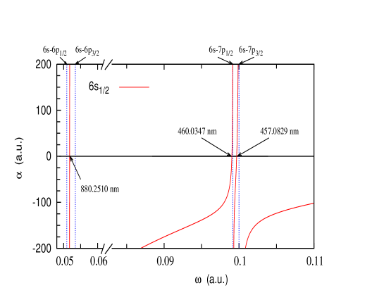
Figure 1: Dynamic polarizabilities of the ground state of Cs atoms. Three visible tune-out wavelengths are found, which are marked with arrows. Approximate positions of the $6s_{1/2}\to np_{j}$ resonances are indicated by vertical dotted lines.

III Calculations for the hyperfine components of the ground level of ¹³³Cs

III.1 Energies and reduced matrix elements

In order to further consider the effect of the hyperfine interaction on the polarizabilities, the theory of energies and reduced matrix elements should be reformulated. The energy of a hyperfine state is given by

$$E^{\rm hf}=E_{J}+W_{F},$$ (8)

where $E_{J}$ is the energy of an unperturbed fine-structure level. $W_{F}$ represents the hyperfine interaction energy, which can be expressed as

$$W_{F}=\frac{1}{2}AR+B\frac{\frac{3}{2}R(R+1)-2I(I+1)J(J+1)}{2I(2I-1)2J(2J-1)},$$ (9)

where A and B denote the hyperfine structure constants, $I$ is the nuclear spin ($I$ = 7/2 for ¹³³Cs), and $J$ is total angular momentum of fine-structure energy levels. $R$ is given by

$$R=F(F+1)-I(I+1)-J(J+1)$$ (10)

with total angular momentum $F$ of hyperfine-structure energy levels.

In Table 7, we list the hyperfine structure constants A and B, the hyperfine interaction energies, and the hyperfine energy levels.

Table 7: The hyperfine structure constants A and B, hyperfine interaction energies, and hyperfine energies of some low-lying states of ¹³³Cs atoms. The notation a[b] represents a$\times 10^{b}$.

States	$J$	A (MHz)	B (MHz)	F	$W_{F}$ (a.u.)	$E^{\rm{hf}}$ (a.u)
$6s$	1/2	2298.157943 Williams et al. (2018); Carr and Saffman (2016)		3	$-$7.858[$-$7]	$-$0.14309918241
				4	$+$6.112[$-$7]	$-$0.14309778529
$6p$	1/2	291.9309(12) Gerginov et al. (2006)		3	$-$9.982[$-$8]	$-$0.09216655791
				4	$+$7.764[$-8$]	$-$0.09216638044
	3/2	50.28825(23) Johnson et al. (2004)	$-$0.4940(17) Johnson et al. (2004); Carr and Saffman (2016)	2	$-$5.163[$-$8]	$-$0.08964212213
				3	$-$2.865[$-8$]	$-$0.08964209915
				4	$+$1.946[$-9$]	$-$0.08964206855
				5	$+$4.011[$-8$]	$-$0.08964203039
$7p$	1/2	94.35(4) Feiertag et al. (1972)		3	$-$3.226[$-$8]	$-$0.04389478454
				4	$+$2.509[$-$8]	$-$0.04389472718
	3/2	16.609(5) Belin et al. (1976)	$-$0.15(3) S. et al. (1969)	2	$-$1.705[$-$8]	$-$0.04306790886
				3	$-$9.460[$-$8]	$-$0.04306790127
				4	$+$0.642[$-$9]	$-$0.04306789117
				5	$+$1.324[$-$8]	$-$0.04306787856

By means of the Wigner-Eckart theorem, the transition matrix elements between two hyperfine states $|\gamma_{i}J_{i}IF_{i}\rangle$ and $|\gamma_{g}J_{g}IF_{g}\rangle$ can be written as

$$T^{\rm hf}_{ig}=\langle\gamma_{i}J_{i}IF_{i}\|\bm{D}\|\gamma_{g}J_{g}IF_{g}\rangle$$

$$=(-1)^{I+J_{g}+F_{i}+1}\times\hat{F}_{i}\hat{F}_{g}\left\{\begin{array}[]{ccc}I&J_{i}&F_{i}\\ 1&F_{g}&J_{g}\\ \end{array}\right\}T_{ig}.$$ (13)

In this expression, $\hat{F}=\sqrt{2F+1}$.

Table 8: Partial derivatives (in a.u.) of the matrix elements of the $6s_{1/2}-6p_{1/2,3/2}$ transitions with respect to the initial- and final-state binding energies. The uncertainties are given in parentheses.

Transitions	$\frac{\partial T}{\partial E_{6s}}$	$\frac{\partial T}{\partial E_{j}}$
6$s_{1/2}\rightarrow 6p_{1/2}$	34.82(42)	$-$0.98(4)
6$s_{1/2}\rightarrow 6p_{3/2}$	51.76(62)	$-$7.50(30)

III.2 Dipole polarizabilities

The calculation of dipole scalar polarizabilities for the hyperfine states is rather similar to Eq. (6), except that $f_{0\rightarrow n}$ should be replaced by the hyperfine oscillator strengths $f^{\rm hf}_{g\rightarrow i}$, and $\Delta E_{0\rightarrow n}$ is replaced by the hyperfine transition energy $\Delta E_{g\rightarrow i}$. Likewise, the calculation of hyperfine absorption oscillator strength $f^{\rm hf}_{g\rightarrow i}$ is similar to Eq. (7) except that $J_{0}$ should be replaced by $F$ and the matrix element is replaced by Eq. (13). Because the total angular momentum of the hyperfine components of the ground level is greater than one, the corresponding dipole polarizability has a tensor component, which can be written as

$$\alpha^{\rm T}(\omega)=6\left(\frac{5F_{g}(2F_{g}-1)(2F_{g}+1)}{6(F_{g}+1)(2F_{g}+3)}\right)^{1/2}$$ (16)

$$\times \sum_{i}(-1)^{F_{g}+F_{i}}\left\{\begin{array}[]{ccc}F_{g}&1&F_{i}\\ 1&F_{g}&2\\ \end{array}\right\}\frac{f^{\rm hf}_{g\rightarrow i}}{\Delta E_{g\rightarrow i}^{2}-\omega^{2}}.$$

Here, $\Delta E_{g\rightarrow i}=E^{\rm hf}_{i}-E^{\rm hf}_{g}$. The total polarizability of a hyperfine state is written as

$$\alpha_{M_{F_{g}}}(\omega)=\alpha^{S}(\omega)+\alpha^{T}(\omega)\frac{3M_{g}^{2}-F_{g}(F_{g}+1)}{F_{g}(2F_{g}-1)},$$ (17)

in which $M_{F_{g}}$ is the magnetic component of the quantum number $F_{g}$.

In the calculations of polarizabilities, small corrections to the matrix elements of the $6s_{1/2}\rightarrow 6p_{1/2,3/2}$ transitions are made, which are treated as parametric functions of the binding energies of the lower and upper levels and can be written as

$$T^{c}_{6s_{1/2},{6p_{j}}}\approx T_{6s_{1/2},{6p_{j}}}+\frac{\partial T_{{6s_{1/2}},6p_{j}}}{\partial E_{6s_{1/2}}}W_{F_{6s_{1/2}}}$$ (18)

$$+\frac{\partial T_{{6s_{1/2}},{6p_{j}}}}{\partial E_{6p_{j}}}W_{F_{6p_{j}}},$$

where $T_{6s_{1/2},6p_{j}}$ denotes the $6s_{1/2}\rightarrow 6p_{1/2,3/2}$ transition matrix elements, and $W_{F}$ are defined by Eq. 9. The partial derivatives denote the ratio of the changes in the reduced matrix elements and binding energies. In the present calculations, we repeat the calculations of these derivatives many times, each time using a slightly different polarization potential (with the change of binding energy in the range $10^{-9}$-$10^{-5}$ a.u.). Table 8 lists the average values of these partial derivatives and the corresponding uncertainties that are determined as root-mean-squares (rms) of the differences from the average values. Then, the dipole polarizabilities for the hyperfine states are further determined by using these partial derivatives.

Table 9 lists the dipole scalar and tensor polarizabilities of the hyperfine components of the ground level of ¹³³Cs. The uncertainties are derived from the uncertainties of the partial derivatives in Table 8. The tensor polarizabilities of the hyperfine states are found to be $10^{-4}$ in magnitude. As far as we know, there are no other theoretical or experimental results for direct comparison. Nevertheless, we can compare the present hyperfine Stark shift of the ground states with other available results Feichtner et al. (1965); Lee et al. (1975); Pal’chikov et al. (2003); Micalizio et al. (2004); Angstmann et al. (2006); Haun and Zacharias (1957); Mowat (1972); Bauch and Schröder (1997); Simon et al. (1998); Levi et al. (2004); Godone et al. (2005). It is often reported in experiment as a hyperfine Stark shift coefficient $k$ (in Hz/(V/m)²), i.e., $k=-0.5\Delta\alpha$ with the difference $\Delta\alpha$ in the scalar polarizabilities of the hyperfine components $F$=4 and $F$=3 of the ground level. Table 10 lists the hyperfine Stark shift coefficient $k$ and $\Delta\alpha$. As can be seen from this table, the present hyperfine Stark shift agrees very well with other experimental Haun and Zacharias (1957); Mowat (1972); Simon et al. (1998); Levi et al. (2004); Godone et al. (2005); Bauch and Schröder (1997) and theoretical results Feichtner et al. (1965); Pal’chikov et al. (2003); Micalizio et al. (2004); Angstmann et al. (2006); Beloy et al. (2006); Lee et al. (1975).

The correction of Eq. (14) to the $6s_{1/2}\rightarrow 6p_{j}$ transition matrix elements is very significant for the result of the hyperfine Stark shift. The $\Delta\alpha$ without considering the correction of the transition matrix elements is just $-$0.01013 a.u. That is, the correction of the $6s_{1/2}\rightarrow 6p_{1/2,3/2}$ transition matrix elements makes the hyperfine Stark shift increase by about 85%.

Table 9: Dipole scalar $\alpha^{S}$ and tensor $\alpha^{T}$ polarizabilities of the hyperfine components of the ground level of ¹³³Cs. The uncertainties are given in parentheses. a[b] represents a$\times 10^{b}$.

States	$F$	$\alpha^{S}$ (a.u)	$\alpha^{T}$ (a.u.)
6s1/2	3	400.66237(3)	1.2263(24)[$-$4]
6s1/2	4	400.68105(3)	$-$2.2919(45)[$-$4]

Table 10: Hyperfine Stark shift coefficients $k$ (in Hz/(V/m)²) and the differences $\Delta\alpha$ (in a.u.) in the scalar polarizabilities of the hyperfine components of the ground level $F$=4 and $F$=3. The unit Hz/(V/m)² can be converted into a.u. by multiplying $0.4018778\times 10^{8}$. The uncertainties are given in parentheses.

Methods	$\Delta\alpha$	$k~{}(\times 10^{-10}$ )
RCICP	0.01868(4)	$-$2.324(5)
MBPT Feichtner et al. (1965)	0.0153(24)	$-$1.9(3)
MBPT Lee et al. (1975)	0.017925	$-$2.2302
MCDF Pal’chikov et al. (2003)	0.018325	$-$2.28
$ab~{}initio$ Micalizio et al. (2004)	0.01583(72)	$-$1.97(9)
$ab~{}initio$ Angstmann et al. (2006)	0.01817(16)	$-$2.26(2)
Relativistic many-body  Beloy et al. (2006)	0.018253(65)	$-$2.271(8)
Perturbation theory Ulzega et al. (2006)	0.01656(8)	$-$2.06(1)
Expt. Haun and Zacharias (1957)	0.01841(56)	$-$2.29(7)
Expt. Mowat (1972)	0.01809(40)	$-$2.25(5)
Expt. Bauch and Schröder (1997)	0.01744(209)	$-$2.17(26)
Expt. Simon et al. (1998)	0.018253(32)	$-$2.271(4)
Expt. Levi et al. (2004)	0.01519 (96)	$-$1.89(12)
Expt. Godone et al. (2005)	0.01632(32)	$-$2.03(4)

Table 11: Tune-out wavelengths $\lambda_{\rm zero}$ (nm) of the $6s_{1/2},F$=3, 4 states of ¹³³Cs atoms. $\Delta\lambda$ denotes the shifts of the primary tune-out wavelengths relative to the tune-out wavelengths of the $6s_{1/2}$ state. $\Delta E$ denotes the corresponding energy shifts.

$F$=3			$F$=4
$\lambda_{\rm zero}$	$\Delta\lambda~{}(10^{-2}$ nm)	$\Delta E~{}(10^{-7}$ a.u.)	$\lambda_{\rm zero}$	$\Delta\lambda~{}(10^{-2}$ nm)	$\Delta E~{}(10^{-7}$ a.u.)
894.58011017(6)	–	–	894.60361080(6)	–	–
880.2008518(18)	$-$1.35482(18)	7.9965(10)	880.2250251(18)	1.06251(18)	$-$6.2194(10)
852.33538210(7)	–	–	852.35737909(7)	–	–
852.33485022(7)	–	–	852.35675635(7)	–	–
460.2117478(5)	$-$0.36522(5)	7.9440(9)	460.2182931(5)	0.28931(5)	$-$6.1364(9)
459.44234414(4)	–	–	459.44872828(4)	–	–
457.2468549(4)	$-$0.35451(4)	7.7871(8)	457.2531880(4)	0.27880(4)	$-$6.0143(8)
455.65213817(3)	–	–	455.65847816(3)	–	–
455.65208799(3)	–	–	455.65841938(3)	–	–

Table 12: Tune-out wavelengths $\lambda_{\rm zero}$ (nm) of the magnetic sublevels of the $6s_{1/2},F$=3, 4 states of ¹³³Cs atoms. $\Delta\lambda$ (nm) is the difference of the tune-out wavelengths with and without considering the tensor contributions.

$\lambda_{\rm zero}$	$\Delta\lambda$	$\lambda_{\rm zero}$	$\Delta\lambda$
$F=3$
$M_{\rm F}=\pm 3$		$M_{\rm F}=\pm 2$
880.2009172(18)	6.54$\times 10^{-5}$	880.2008518(18)	$\textless 10^{-7}$
460.2117558(5)	8.00$\times 10^{-6}$	460.2117478(4)	$\textless 10^{-7}$
457.2468553(4)	0.40$\times 10^{-6}$	457.2468548(4)	$\textless 10^{-7}$
$M_{\rm F}=\pm 1$		$M_{\rm F}=\pm 0$
880.2008126(17)	$-$3.92$\times 10^{-5}$	880.2007995(17)	$-$5.23$\times 10^{-5}$
460.2117432(2)	$-$4.62$\times 10^{-6}$	460.2117415(3)	$-$6.30$\times 10^{-6}$
457.2468547(2)	$-$0.20$\times 10^{-6}$	457.2468546(3)	$-$0.30$\times 10^{-6}$
$F=4$
$M_{\rm F}=\pm 4$		$M_{\rm F}=\pm 3$
880.2249277(18)	$-$9.74$\times 10^{-5}$	880.2250007(18)	$-$2.44$\times 10^{-5}$
460.2182814(5)	$-$1.17$\times 10^{-5}$	460.2182902(4)	3.00$\times 10^{-6}$
457.2531875(4)	$-$0.50$\times 10^{-6}$	457.2531878(4)	$-$0.20$\times 10^{-6}$
$M_{\rm F}=\pm 2$		$M_{\rm F}=\pm 1$
880.2250529(17)	2.78$\times 10^{-5}$	880.2250842(17)	6.00$\times 10^{-5}$
460.2182964(2)	$-$3.30$\times 10^{-6}$	460.2183002(3)	7.10$\times 10^{-6}$
457.2531882(2)	0.20$\times 10^{-6}$	457.2531883(3)	0.20$\times 10^{-6}$
$M_{\rm F}=\pm 0$
880.2250946(17)	6.95$\times 10^{-5}$
460.2183015(2)	8.40$\times 10^{-6}$
457.2531884(2)	0.40$\times 10^{-6}$

III.3 Tune-out wavelengths

By means of the hyperfine energy levels and matrix elements obtained above, the dynamic polarizabilities and tune-out wavelengths of the hyperfine components of the ground level can be further determined. Table 11 lists the tune-out wavelengths of the hyperfine components of the ground level of ¹³³Cs, in which the tensor contribution is not considered. Two new features of the tune-out wavelengths are found for the hyperfine splitting. One of them is that the hyperfine splitting of the ground state results in two sets of tune-out wavelengths; one is for the 6$s_{1/2},F$ = 3 state, and the other is for the 6$s_{1/2},F=4$ state. Another feature is that the hyperfine splitting of the $np_{j}$ states results in additional tune-out wavelengths. The tune-out wavelengths near 894 nm and 852 nm are located between the hyperfine components of the transitions from the $6p_{1/2}$ and $6p_{3/2}$ levels to the ground level, respectively, while the ones near 459 nm and 455 nm are located between the hyperfine components of the transitions from the 7$p_{1/2}$ and 7$p_{3/2}$ levels to the ground level, respectively. These tune-out wavelengths would be difficult to be measured in experiments due to very small energy splittings of the hyperfine states. The tune-out wavelength near 880 nm is the first primary tune-out wavelength, which lies between the excitation thresholds of the $6p_{1/2}$ and $6p_{3/2}$ states. The primary tune-out wavelength 880.200852 nm of the 6$s_{1/2},F=3$ state is shorter than the 880.2144 nm tune-out wavelength of the 6$s_{1/2}$ state by about 0.013548 nm. The tune-out wavelength 880.225025 nm of the 6$s_{1/2},F=4$ state is longer than the 880.2144 nm tune-out wavelength of the 6$s_{1/2}$ state by about 0.010625 nm. As can be seen from Table 11, the energy shifts of the first primary tune-out wavelengths for the $6s_{1/2},F=3,4$ states are 7.997 $\times 10^{-7}$ a.u. and $-$6.219 $\times 10^{-7}$ a.u., respectively. These shifts correspond very closely to the hyperfine interaction energies of the $6s_{1/2}$ state. The tune-out wavelengths near 460 nm and 457 nm are also primary tune-out wavelengths, which lie between the excitation thresholds of the 6$p_{3/2}$ and 7$p_{1/2}$ states and the thresholds of the 7$p_{1/2}$ and 7$p_{3/2}$ states, respectively. The energy shifts of the tune-out wavelengths are also very close to the hyperfine interaction energy of the ground state.

While the calculations of the hyperfine Stark shift are critically reliant on the use of the energy-adjusted reduced dipole matrix elements, this is not true for the tune-out wavelengths. For example, the difference of the tune-out wavelengths near 880 nm with and without considering the correction to the 6$s_{1/2}\rightarrow 6p_{1/2,3/2}$ transition matrix elements are only $-$8.5$\times 10^{-5}$ nm and $-$6$\times 10^{-6}$ nm for the $F=3$ and $F=4$ states, respectively. The influence of the correction to the transition matrix elements on the tune-out wavelengths can be ignored.

If tensor polarizabilities are considered, the tune-out wavelengths also depend on the magnetic sublevels. Table 12 lists the primary tune-out wavelengths for the magnetic sublevels of the $6s_{1/2}$ $F=3$ and $F=4$ states of ¹³³Cs. The differences of the tune-out wavelengths with and without considering the tensor contributions are also listed in Table 12. It is found that the differences in these tune-out wavelengths for any of the magnetic sublevels are $10^{-5}\sim 10^{-6}$ nm. If the tune-out wavelengths could be measured at a level of fm, the contribution of the tensor polarizabilities to the tune-out wavelengths could be extracted from experiments.

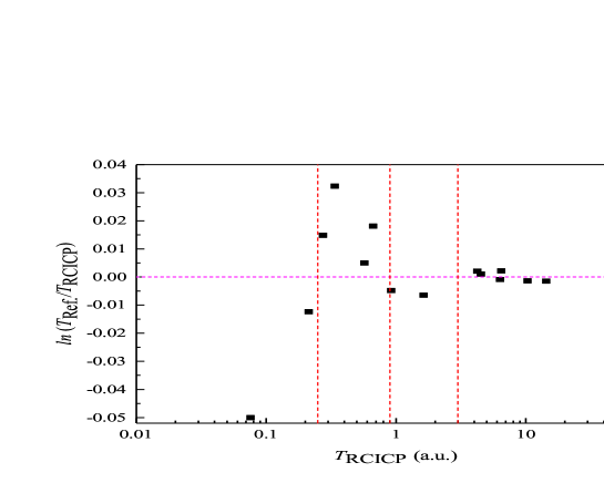
Figure 2: Natural logarithm of the ratio, ln ($T_{\rm Ref}/T_{\rm RCICP}$).

IV Remarks on uncertainty of the present results

The uncertainties of the present transition matrix elements $T_{RCICP}$ given in Table 3 are estimated very carefully. Similar to the method used in Ref. Kramida (2013), in which the oscillator strengths are classified into different groups based on the deviations from best experimental data, the uncertainties of the RCICP transition matrix elements are evaluated by comparing with the most accurate experimental or theoretical resutls $T_{\rm Ref}$ listed in bold in Table 3. FIG. 2 plots the natural logarithm of the ratio, ln($T_{\rm Ref}/T_{\rm RCICP}$). As shown in this figure, the matrix elements of all the involved transitions can be classified into four groups. The first group is those with the $T_{\rm RCICP}$ larger than 3.0 a.u., which consists of the ${6s_{1/2}\rightarrow 6p_{1/2,3/2}}$, $7s_{1/2}\rightarrow 6p_{1/2,3/2}$, and $7s_{1/2}\rightarrow 7p_{1/2,3/2}$ transitions. These transition matrix elements are calculated very accurately. The uncertainty estimated by the rms of the difference from the reference values is about 0.17% for this group. The second group is those with the $T_{\rm RCICP}$ in the range 0.9–3.0 a.u., including the ${7s_{1/2}\rightarrow 8p_{1/2,3/2}}$ transitions. The uncertainty for this group is about 0.6%. The third group is those with the $T_{\rm RCICP}$ in the range 0.25–0.9 a.u., including the ${6s_{1/2}\rightarrow 7p_{1/2,3/2}}$ and ${7s_{1/2}\rightarrow 9p_{1/2,3/2}}$ transitions. The uncertainty is about 2%. The fourth group is those with the $T_{\rm RCICP}$ smaller than 0.25 a.u., including the ${6s_{1/2}\rightarrow 8p_{1/2,3/2}}$ transitions. The uncertainty is about 3.6%. It should be mentioned that the uncertainties given above are estimated on the level of one standard deviation.

However, the uncertainties of the tune-out wavelengths need to be specially considered due to different transition contributions. For the tune-out wavelength near 880 nm, its calculation can be simplified as

$$0=\frac{f_{6s_{1/2}\rightarrow 6p_{1/2}}}{(\Delta E^{2}_{6s_{1/2}\rightarrow 6p_{1/2}}-\omega^{2})}+\frac{f_{6s_{1/2}\rightarrow 6p_{1/2}}\mathcal{R}_{6p}(1+\delta_{6p})}{[(\Delta E^{2}_{6s_{1/2}\rightarrow 6p_{1/2}})(1+\delta_{6p})^{2}-\omega^{2}]}$$

$$+\alpha_{rem}(\omega).$$ (19)

Here, $\mathcal{R}_{6p}$=${|\langle 6s_{1/2}||D||6p_{3/2}\rangle|^{2}}/{|\langle 6s_{1/2}||D||6p_{1/2}\rangle|^{2}}$, and $\alpha_{rem}(\omega)$ is the remainder part (exclude the $6s_{1/2}\rightarrow 6p_{1/2,3/2}$) of dynamic dipole polarizability. The energy difference $\Delta E^{2}_{6p_{3/2}}$ can be expressed as $\Delta E^{2}_{6p_{3/2}}\!=\!\Delta E^{2}_{6p_{1/2}}$(1+$\delta_{6p})^{2}$ with $\delta_{6p}$=0.0495639. As seen from Eq. (IV), there are three sources of the uncertainty for this tune-out wavelength. The first source is the uncertainty of the $6s_{1/2}\rightarrow 6p_{1/2}$ reduced matrix element or oscillator strengths. The uncertainty 0.17% of the $6s_{1/2}\rightarrow 6p_{1/2}$ matrix elements may lead to an uncertainty of 0.0004 nm for the 880-nm tune-out wavelength. The second one is the uncertainty of the line strength ratio $\mathcal{R}_{6p}$. We find that this tune-out wavelength is very sensitive to the ratio $\mathcal{R}_{6p}$. The uncertainty of the RCICP ratio $\mathcal{R}_{6p}$ = 1.9844(100) leads to an uncertainty of 0.0475 nm for this tune-out wavelength. The third one is the uncertainty of the $\alpha_{rem}(\omega)$. The uncertainty of the $\alpha_{rem}(\omega)$, which includes the uncertainties of the $\alpha_{core}$ and transitions from more highly-excited states (assumed to be 10% uncertainty), may lead to an uncertainty of 0.0005 nm for this tune-out wavelength. By comparing the above estimations, it can be found that the total uncertainty of the 880-nm tune-out wavelength is mainly determined by the uncertainty of the $\mathcal{R}_{6p}$, and the uncertainties from the uncertainties of the $6s_{1/2}\rightarrow 6p_{1/2}$ transition matrix element and $\alpha_{rem}(\omega)$ are negligible. For the 880-nm $\lambda_{\rm zero}^{recom}$, the uncertainty of the experimental line strength ratio ($\mathcal{R}_{6p}=1.9768(33))$ leads to an uncertainty of 0.0158 nm, which is about one third of the uncertainty of the RCICP tune-out wavelength.

Moreover, as for the tune-out wavelengths near 460 nm and 457 nm, both of them are caused by a cancellation of the $6s_{1/2}\rightarrow 6p_{1/2,3/2}$ and $6s_{1/2}\rightarrow 7p_{1/2,3/2}$ transitions. The corresponding calculation can be simplified as

$$0=\alpha_{6p}(\omega)+\frac{f_{6s_{1/2}\rightarrow 7p_{1/2}}}{(\Delta E^{2}_{7p_{1/2}}-\omega^{2})}+\frac{f_{{6s_{1/2}\rightarrow 7p_{1/2}}}\mathcal{R}_{7p}(1+\delta_{7p})}{[(\Delta E^{2}_{7p_{1/2}})(1+\delta_{7p})^{2}-\omega^{2}]}$$

$$+\alpha^{\prime}_{rem}(\omega),$$ (20)

where $\mathcal{R}_{7p}={|\langle 6s_{1/2}||D||7p_{3/2}\rangle|^{2}}/{|\langle 6s_{1/2}||D||7p_{1/2}\rangle|^{2}}$. $\alpha^{\prime}_{rem}(\omega)$ is the remainder part (exclude the $6s_{1/2}\rightarrow 6p_{1/2,3/2}$ and $6s_{1/2}\rightarrow 7p_{1/2,3/2}$ ) of dynamic dipole polarizability. The polarizability $\alpha_{6p}(\omega)$ corresponding to the $6s_{1/2}\rightarrow 6p_{1/2,3/2}$ transitions is retained as a separate term since it is much larger than the remainder term. The uncertainty analysis of these two tune-out wavelengths is similar to the analysis of the 880-nm tune-out wavelength. The uncertainties of the RCICP $\alpha_{6p}(\omega)$ and the $6s_{1/2}\rightarrow 7p_{1/2}$ matrix elements lead to the uncertainties of 0.0043 nm and 0.0468 nm for these tune-out wavelengths. The uncertainty of the RCICP ratio $\mathcal{R}_{7p}$ = 4.3474(2463) leads to the uncertainties of 0.0271 nm and 0.0783 nm for 460-nm and 457-nm tune-out wavelengths, respectively. Consequently, the total uncertainties (arithmetic square root of the sum of squares of those uncertainties) of the RCICP 460-nm and 457-nm tune-out wavelength are estimated to be about 0.0543 nm and 0.0917 nm. However, for the 460-nm and 457-nm $\lambda_{\rm zero}^{recom}$, the uncertainty of the experimental $\alpha_{6p}(\omega)$, which were derived from the uncertainty of the experimental transition matrix elements of the $6s_{1/2}\rightarrow 6p_{1/2,3/2}$, leads to an uncertainty of 0.0014 nm. The uncertainty of the $6s_{1/2}\rightarrow 7p_{1/2}$ matrix element makes an uncertainty of 0.0039 nm. The experimental ratio $\mathcal{R}_{7p}$ = 4.2626(396) leads to the uncertainties of 0.0047 nm and 0.0132 nm for the 460-nm and 457-nm $\lambda_{\rm zero}^{recom}$, respectively. As a result, the total uncertainties of the 460-nm and 457-nm $\lambda_{\rm zero}^{recom}$ are about 0.0063 nm and 0.0171nm.

Apart from the uncertainty corresponding to the fine-structure states, the uncertainty of tune-out wavelengths of the hyperfine states should be stated as well. The source of the uncertainties of the tune-out wavelengths for the hyperfine components of the ground level should include two parts. The first part is from the uncertainties of the matrix elements in Table 3. The uncertainties for the primary tune-out wavelengths (near 880, 460 and 457 nm) derived from this part are expected to be at the same level as those of the tune-out wavelengths of the fine-structure $6s_{1/2}$ state. The second part is from the uncertainties of the partial derivatives in Table 8. This part is the main source for the uncertainties of the tune-out wavelength shifts $\Delta\lambda$ in Table 11. In order to show the uncertainties of the $\Delta\lambda$s , Table 11 lists the uncertainties that are derived from the uncertainties of the partial derivatives. However, for the tune-out wavelengths near the 894, 852, 459 and 455 nm, which are located between the transition energies from the hyperfine components of the $6p_{1/2}$, $6p_{3/2}$, $7p_{1/2}$ and $7p_{3/2}$ to the $6s_{1/2}$ $F=3$ (or $F=4$) levels, the uncertainties are estimated to be less than $10^{-7}$ nm.

V CONCLUSION

The energy levels, E1 transition matrix elements, static and dynamic polarizabilities corresponding to the $6s_{1/2}$ state of Cs atoms are calculated by using the RCICP approach. Three longest tune-out wavelengths of the $6s_{1/2}$ state are determined. It has been found that the present RCICP results agree very well with other available experimental and theoretical results.

Apart from the fine-structure $6s_{1/2}$ state, in particular, we consider the effect of the hyperfine splittings of the $6s_{1/2}$, 6$p_{j}$, and 7$p_{j}$ states of ¹³³Cs atoms. The dynamic polarizabilities and tune-out wavelengths of the hyperfine components of the ground level of ¹³³Cs atoms are further determined. The tune-out wavelengths corresponding to the hyperfine splittings of the $np_{j}$ states are hard to be measured. However, all of the obtained primary tune-out wavelengths have relatively large hyperfine shifts. For example, the shifts of the 880-nm tune-out wavelength corresponding to the 6$s_{1/2},F=3$ and $F=4$ states are about $-$0.0135 nm and 0.0106 nm, respectively; they are very close to the hyperfine interaction energies. Such large shifts can be resolved in experiments. If the tune-out wavelengths could be measured at a level of fm, the contribution of the tensor polarizabilities of the hyperfine components of the ground level to the tune-out wavelengths could be extracted from experiments. In addition, the 880-nm tune-out wavelength is found to be very sensitive to the ratio of the line strengths of the $6s_{1/2}\to 6p_{1/2,3/2}$ transitions. Accurate measurements on this tune-out wavelength would enable a high-precision determination of the $6s_{1/2}\to 6p_{1/2,3/2}$ line strength ratio.

VI ACKNOWLEDGMENTS

This work has been supported by the National Key Research and Development Program of China under Grant No. 2017YFA0402300 and the National Natural Science Foundation of China under Grant Nos. 11774292, 11564036, 11804280, 11874051, and 11864036. Z. W. W. acknowledges the Major Project of the Research Ability Promotion Program for Young Scholars of Northwest Normal University of China under Grant No. NWNU-LKQN2019-5. We are very grateful to the anonymous referees for their constructive comments on this work.

References

- Grimm et al. (2000) R. Grimm, M. Weidemüller, and Y. B. Ovchinnikov, Adv. At. Mol. Opt. Phys. 42, 95 (2000).
- Leblanc and Thywissen (2007) L. J. Leblanc and J. H. Thywissen, Phys. Rev. A 75, 053612 (2007).
- Luan et al. (2015) T. Luan, H. Yao, L. Wang, C. Li, S. Yang, X. Chen, and Z. Ma, Opt. Express 23, 11378 (2015).
- Chamakhi et al. (2015) R. Chamakhi, H. Ahlers, M. Telmini, C. Schubert, E. M. Rasel, and N. Gaaloul, New J. Phys. 17, 123002 (2015).
- Catani et al. (2009) J. Catani, G. Barontini, G. Lamporesi, F. Rabatti, G. Thalhammer, F. Minardi, S. Stringari, and M. Inguscio, Phys. Rev. Lett. 103, 140401 (2009).
- Herold et al. (2012) C. D. Herold, V. D. Vaidya, X. Li, S. L. Rolston, J. V. Porto, and M. S. Safronova, Phys. Rev. Lett. 109, 243003 (2012).
- Safronova et al. (2015) M. S. Safronova, Z. Zuhrianda, U. I. Safronova, and C. W. Clark, Phys. Rev. A 92, 040501 (2015).
- Fallon and Sackett (2016) A. Fallon and C. Sackett, Atoms 4, 12 (2016).
- Holmgren et al. (2012) W. F. Holmgren, R. Trubko, I. Hromada, and A. D. Cronin, Phys. Rev. Lett. 109, 243004 (2012).
- Leonard et al. (2015) R. H. Leonard, A. J. Fallon, C. A. Sackett, and M. S. Safronova, Phys. Rev. A 92, 052501 (2015).
- Leonard et al. (2017) R. H. Leonard, A. J. Fallon, C. A. Sackett, and M. S. Safronova, Phys. Rev. A 95, 059901 (2017).
- Henson et al. (2015) B. M. Henson, R. I. Khakimov, R. G. Dall, K. G. H. Baldwin, L.-Y. Tang, and A. G. Truscott, Phys. Rev. Lett. 115, 043004 (2015).
- Mitroy and Tang (2013) J. Mitroy and L.-Y. Tang, Phys. Rev. A 88, 052515 (2013).
- Copenhaver et al. (2019) E. Copenhaver, K. Cassella, R. Berghaus, and H. Müller, Phys. Rev. A 100, 063603 (2019).
- Monroe et al. (1995) C. Monroe, D. M. Meekhof, B. E. King, W. M. Itano, and D. J. Wineland, Phys. Rev. Lett. 75, 4714 (1995).
- Jefferts et al. (2014) S. R. Jefferts, T. P. Heavner, T. E. Parker, J. H. Shirley, E. A. Donley, N. Ashby, F. Levi, D. Calonico, and G. A. Costanzo, Phys. Rev. Lett. 112, 050801 (2014).
- Wang et al. (2015) Y. Wang, X. Zhang, T. A. Corcovilos, A. Kumar, and D. S. Weiss, Phys. Rev. Lett. 115, 043003 (2015).
- Arora et al. (2011) B. Arora, M. S. Safronova, and C. W. Clark, Phys. Rev. A 84, 043401 (2011).
- Mitroy and Bromley (2003) J. Mitroy and M. W. J. Bromley, Phys. Rev. A 68, 52714 (2003).
- Grant (2007) I. P. Grant, Relativistic Quantum Theory of Atoms and Molecules Theory and Computation (Springer, New York, 2007).
- Grant and Quiney (1988) I. P. Grant and H. M. Quiney, Adv. At. Mol. Phys 23, 37 (1988).
- Grant (1989) I. P. Grant, Relativistic, Quantum Electrodynamic and Weak Interaction Effects in Atoms, edited by P.J.Mohr, W. R. Johnson, and J. Sucher, AIP Conf. Proc. No. 189 (AIP, New York) , pp. 235 (1989).
- Grant (1996) I. P. Grant, Advance Atom, Molecular and Optical Physics Reference Book, edited by G. W. F. Drake (AIP, New York Chap. 22 (1996).
- Lim et al. (2002) I. Lim, J. Laerdahl, and P. Schwerdtfeger, J. Chem. Phys. 116, 172 (2002).
- Johnson et al. (1983) W. R. Johnson, D. Kolb, and K. N. Huang, At. Data Nucl. Data Tables 28, 333 (1983).
- Grant and Quiney (2000) I. P. Grant and H. M. Quiney, Phys. Rev. A 62, 022508 (2000).
- Mitroy and Bromley (2003) J. Mitroy and M. W. Bromley, Phys. Rev. A 68, 052714 (2003).
- (28) A. Kramida, Yu. Ralchenko, J. Reader, and and NIST ASD Team, NIST Atomic Spectra Database (Ver. 5.7.1),2019, [Online]. Available: https://physics.nist.gov/asd.
- (29) M. S. Safronova, U. I. Safronova, and C. W. Clark, Phys. Rev. A 94, 012505 (2016), and Supplement Material https://journals.aps.org/pra/supplemental/0.1103/ PhysRevA.94.012505/Suppl.pdf .
- Safronova et al. (1999) M. S. Safronova, W. R. Johnson, and A. Derevianko, Phys. Rev. A 60, 4476 (1999).
- Roberts et al. (2014) B. M. Roberts, V. A. Dzuba, and V. V. Flambaum, Phys. Rev. A 89, 012502 (2014).
- Rafac et al. (1999) R. J. Rafac, C. E. Tanner, A. E. Livingston, and H. G. Berry, Phys. Rev. A 60, 3648 (1999).
- Derevianko and Porsev (2002) A. Derevianko and S. G. Porsev, Phys. Rev. A 65, 053403 (2002).
- Gregoire et al. (2016) M. Gregoire, N. Brooks, R. Trubko, and A. Cronin, Atoms 4, 21 (2016).
- Kien et al. (2013) F. L. Kien, P. Schneeweiss, and A. Rauschenbeutel, Eur. Phys. J. D 67, 1 (2013).
- Blundell et al. (1992) S. A. Blundell, J. Sapirstein, and W. R. Johnson, Phys. Rev. D 45, 1602 (1992).
- Patterson et al. (2015) B. M. Patterson, J. F. Sell, T. Ehrenreich, M. A. Gearba, G. M. Brooke, J. Scoville, and R. J. Knize, Phys. Rev. A 91, 012506 (2015).
- Damitz et al. (2019) A. Damitz, G. Toh, E. Putney, C. E. Tanner, and D. S. Elliott, Phys. Rev. A 99, 062510 (2019).
- Porsev et al. (2010) S. G. Porsev, K. Beloy, and A. Derevianko, Phys. Rev. D 82, 036008 (2010).
- Shabanova et al. (1979) L. N. Shabanova, Y. N. Monakov, and A. N. Khlyustalov, Opt. Spectrosc. 47, 1 (1979).
- Blundell et al. (1991) S. A. Blundell, W. R. Johnson, and J. Sapirstein, Phys. Rev. A 43, 3407 (1991).
- Antypas and Elliott (2013) D. Antypas and D. S. Elliott, Phys. Rev. A 88, 052516 (2013).
- Vasilyev et al. (2002) A. A. Vasilyev, I. M. Savukov, M. S. Safronova, and H. G. Berry, Phys. Rev. A 66, 020101 (2002).
- Toh et al. (2019) G. Toh, A. Damitz, C. E. Tanner, W. R. Johnson, and D. S. Elliott, Phys. Rev. Lett. 123, 073002 (2019).
- Toh et al. (2019) G. Toh, A. Damitz, N. Glotzbach, J. Quirk, I. C. Stevenson, J. Choi, M. S. Safronova, and D. S. Elliott, Phys. Rev. A 99, 032504 (2019).
- Bennett et al. (1999) S. C. Bennett, J. L. Roberts, and C. E. Wieman, Phys. Rev. A 59, R16 (1999).
- Johnson et al. (1996) W. R. Johnson, Z. W. Liu, and J. Sapirstein, At. Data Nucl. Data Tables 64, 279 (1996).
- Johnson et al. (1987) W. R. Johnson, M. Idrees, and J. Sapirstein, Phys. Rev. A 35, 3218 (1987).
- Young et al. (1994) L. Young, I. Hill, W. T., S. J. Sibener, S. D. Price, C. E. Tanner, C. E. Wieman, and S. R. Leone, Phys. Rev. A 50, 2174 (1994).
- Morton (2000) D. C. Morton, The Astro phys. J., Suppl. Ser 130, 403 (2000).
- Exton (1976) R. J. Exton, J. Quant. Spectrosc. Radiat. Transfer 16, 309 (1976).
- Pichler (1976) G. Pichler, J. Quant. Spectrosc. Radiat. Transfer 16, 147 (1976).
- Rafac et al. (1994) R. J. Rafac, C. E. Tanner, A. E. Livingston, K. W. Kukla, H. G. Berry, and C. A. Kurtz, Phys. Rev. A 50, R1976 (1994).
- Bouloufa et al. (2007) N. Bouloufa, A. Crubellier, and O. Dulieu, Phys. Rev. A 75, 052501 (2007).
- Sell et al. (2011) J. F. Sell, B. M. Patterson, T. Ehrenreich, G. Brooke, J. Scoville, and R. J. Knize, Phys. Rev. A 84, 010501 (2011).
- Tanner et al. (1992) C. E. Tanner, A. E. Livingston, R. J. Rafac, F. G. Serpa, K. W. Kukla, H. G. Berry, L. Young, and C. A. Kurtz, Phys. Rev. Lett. 69, 2765 (1992).
- Mitroy et al. (1988) J. Mitroy, D. C. Griffin, D. W. Norcross, and M. S. Pindzola, Phys. Rev. A 38, 3339 (1988).
- Marinescu et al. (1994) M. Marinescu, H. R. Sadeghpour, and A. Dalgarno, Phys. Rev. A 49, 5103 (1994).
- Hameed et al. (1968) S. Hameed, A. Herzenberg, and M. G. James, Journal of Physics B Atomic Molecular Physics 1, 822 (1968).
- Caves and Dalgarno (1972) T. C. Caves and A. Dalgarno, J. Quant. Spectrosc. Radiat. Transfer. 12, 1539 (1972).
- Hafner and Schwarz (1978) P. Hafner and W. H. E. Schwarz, J. Phys. B. 11, 2975 (1978).
- Gregoire et al. (2015) M. D. Gregoire, I. Hromada, W. F. Holmgren, R. Trubko, and A. D. Cronin, Phys. Rev. A 92, 052513 (2015).
- Arora et al. (2007) B. Arora, M. S. Safronova, and C. W. Clark, Phys. Rev. A 76, 052516 (2007).
- Dzuba et al. (1989) V. A. Dzuba, V. V. Flambaum, and O. P. Sushkov, Phys. Lett. A 141, 147 (1989).
- Mitroy et al. (2010) J. Mitroy, M. S. Safronova, and C. W. Clark, J. Phys. B 43, 202001 (2010).
- Derevianko et al. (1999) A. Derevianko, W. R. Johnson, M. S. Safronova, and J. F. Babb, Phys. Rev. Lett. 82, 3589 (1999).
- Singh et al. (2016) S. Singh, K. Kaur, B. K. Sahoo, and B. Arora, J. Phys. B 49, 145005 (2016).
- Iskrenova-Tchoukova et al. (2007) E. Iskrenova-Tchoukova, M. S. Safronova, and U. I. Safronova, J. Comp. Methods in Sci. and Eng. 7, 521 (2007).
- Lim et al. (2005) I. S. Lim, P. Schwerdtfeger, B. Metz, and H. Stoll, J. Chem. Phys. 122, 104103 (2005).
- Borschevsky et al. (2013) A. Borschevsky, V. Pershina, E. Eliav, and U. Kaldor, J. Chem. Phys. 138, 124302 (2013).
- Lim et al. (1999) I. S. Lim, M. Pernpointner, M. Seth, J. K. Laerdahl, P. Schwerdtfeger, P. Neogrady, and M. Urban, Phys. Rev. A 60, 2822 (1999).
- Amini and Gould (2003) J. M. Amini and H. Gould, Phys. Rev. Lett. 91, 153001 (2003).
- Sup (CICP) (See Supplemental Material at http://XXXXXX for additional resutls of RCICP.).
- Williams et al. (2018) W. D. Williams, M. T. Herd, and W. B. Hawkins, Laser. Phys. Lett. 15, 095702 (2018).
- Carr and Saffman (2016) A. W. Carr and M. Saffman, Phys. Rev. Lett. 117, 150801 (2016).
- Gerginov et al. (2006) V. Gerginov, K. Calkins, C. E. Tanner, J. J. McFerran, S. Diddams, A. Bartels, and L. Hollberg, Phys. Rev. A 73, 032504 (2006).
- Johnson et al. (2004) W. R. Johnson, H. C. Ho, C. E. Tanner, and A. Derevianko, Phys. Rev. A 70, 014501 (2004).
- Feiertag et al. (1972) D. Feiertag, A. Sahm, and G. Z. Putlitz, Zeitschrift Für Physik A Hadrons Nuclei 255, 93 (1972).
- Belin et al. (1976) G. Belin, L. Holmgren, and S. Svanberg, Phys. Scr. 14, 39 (1976).
- S. et al. (1969) S., Svanberg, S., and Rydberg, Zeitschrift Für Physik A Hadrons Nuclei 227, 216 (1969).
- Feichtner et al. (1965) J. D. Feichtner, M. E. Hoover, and M. Mizushima, Phys. Rev. 137, 702 (1965).
- Lee et al. (1975) T. Lee, T. P. Das, and R. M. Sternheimer, Phys. Rev. A 11, 1784 (1975).
- Pal’chikov et al. (2003) V. G. Pal’chikov, Y. S. Domnin, and A. V. Novoselov, J. Opt. B 5, S131 (2003).
- Micalizio et al. (2004) S. Micalizio, A. Godone, D. Calonico, F. Levi, and L. Lorini, Phys. Rev. A 69, 053401 (2004).
- Angstmann et al. (2006) E. J. Angstmann, V. A. Dzuba, and V. V. Flambaum, Phys. Rev. A 74, 023405 (2006).
- Haun and Zacharias (1957) R. D. Haun and J. R. Zacharias, Phys. Rev. 107, 107 (1957).
- Mowat (1972) J. R. Mowat, Phys. Rev. A 5, 1059 (1972).
- Bauch and Schröder (1997) A. Bauch and R. Schröder, Phys. Rev. Lett. 78, 622 (1997).
- Simon et al. (1998) E. Simon, P. Laurent, and A. Clairon, Phys. Rev. A 57, 436 (1998).
- Levi et al. (2004) F. Levi, D. Calonico, L. Lorini, S. Micalizio, and A. Godone, Phys. Rev. A 70, 033412 (2004).
- Godone et al. (2005) A. Godone, D. Calonico, F. Levi, S. Micalizio, and C. Calosso, Phys. Rev. A 71, 063401 (2005).
- Beloy et al. (2006) K. Beloy, U. I. Safronova, and A. Derevianko, Phys. Rev. Lett. 97, 040801 (2006).
- Ulzega et al. (2006) S. Ulzega, A. Hofer, P. Moroshkin, and A. Weis, arXive preprint physics/0604233. (2006).
- Kramida (2013) A. Kramida, Fusion. Sci. Technol. 63, 313 (2013).