Optimal Off-Policy Evaluation from
Multiple Logging Policies

Abstract

We study off-policy evaluation (OPE) from multiple logging policies, each generating a dataset of fixed size, i.e., stratified sampling. Previous work noted that in this setting the ordering of the variances of different importance sampling estimators is instance-dependent, which brings up a dilemma as to which importance sampling weights to use. In this paper, we resolve this dilemma by finding the OPE estimator for multiple loggers with minimum variance for any instance, i.e., the efficient one. In particular, we establish the efficiency bound under stratified sampling and propose an estimator achieving this bound when given consistent $q$-estimates. To guard against misspecification of $q$-functions, we also provide a way to choose the control variate in a hypothesis class to minimize variance. Extensive experiments demonstrate the benefits of our methods’ efficiently leveraging of the stratified sampling of off-policy data from multiple loggers.

1 Introduction

In many applications where personalized and dynamic decision making is of interest, exploration is costly, risky, unethical, or otherwise infeasible ruling out the use of online algorithms for contextual bandits (CB) and reinforcement learning (RL) that need to explore in order to learn. This includes both healthcare, where we fear bad patient outcomes, and e-commerce, where we fear alienating users. This motivates the study of off-policy evaluation (OPE), which is the task of estimating the value of a given policy using only historical data, which is generated by current decision policies. This can support performance evaluation of policies with respect to various rewards objectives in order to better understand their behavior before deploying them in a real environment. Given how invaluable this is, OPE has been studied extensively both in CB (Kallus, 2018; Narita et al., 2019; Wang et al., 2017; Dudík et al., 2014; Swaminathan et al., 2017; Muandet et al., 2020; Su et al., 2020) and in RL (Farajtabar et al., 2018; Liu et al., 2018; Kallus and Uehara, 2019a, b, 2020a; Munos et al., 2016; Jiang and Li, 2016; Thomas and Brunskill, 2016; Yin et al., 2020) and has been applied in various domains including healthcare (Murphy, 2003) and education (Mandel et al., 2014).

In most of the above studies, the observations used to evaluate a new policy are assumed generated by a single logging policy. Often, however, we have the opportunity to leverage multiple datasets, each potentially generated by a different logging policy (Agarwal et al., 2017; He et al., 2019; Strehl et al., 2010; Bareinboim and Pearl, 2016). The size of each dataset is generally fixed by design, which distinguishes this setting from a single logging policy given by the mixture of logging policies. Such fixed dataset sizes is an example of stratified sampling (Wooldridge, 2001), where the identity of the logging policies constitute the stratum.

The distinction of these two settings is crucial since the same estimator may have varying precision in each setting (a fact well-known in Monte Carlo integration, Geyer, 1994; Kong et al., 2003; Tan, 2004, and noise contrastive estimation, Gutmann and Hyvärinen, 2010; Uehara et al., 2018). Thus, many results in the standard unstratified OPE setting cannot be directly translated to a multiple logger setting, most crucially the efficiency lower bound on mean-squared error (MSE) and estimators that achieve this lower bound (Narita et al., 2019; Kallus and Uehara, 2020a; Dudík et al., 2014; Jiang and Li, 2016). In the multiple logger setting, we may additionally consider a much greater variety of estimators that can utilize the logger identity as data. In this paper, we study a wide range of such estimators, establish the efficiency lower bound, and propose estimators that achieve it.

Previous work on OPE with multiple loggers proposed various importance sampling (IS) estimators that use the logger identity (Agarwal et al., 2017). However, they arrived at a dilemma: there is no strict ordering between the IS estimate with marginalized logging probabilities and a precision-weighted combination of the IS estimates in each dataset. That is, which estimate has lower MSE depends on the problem instance and is not known a priori, and therefore it is not clear which should be preferred. Our analysis resolves this dilemma by developing an efficient estimator, which has MSE better (or not worse) than both of the above.

Our contributions are as follows. First, when the logging policies are known, we study the variances of a new class of unbiased estimators that includes and is much bigger than the class considered in Agarwal et al. (2017). This new class incorporates both control variates and flexible weights that may depend on logger identity. We show that a single estimator has minimum variance in this class (Sections 3.1 and 3.2). We extend this finite-sample bound to also bound the asymptotic MSEs of all regular estimators, thereby establishing the efficiency lower bound (Section 3.3). We show how to construct an efficient estimator even if behavior policies are unknown and establish theoretical guarantees for it (Section 4). Then, we theoretically investigate the differences between OPE in the stratified and unstratified cases by showing that the variances of the estimator are generally different under two settings and are asymptotically equivalent only when the estimator is efficient (Section 5). We use this insight to choose optimal control variates to directly minimize variance, extending the More Robust Doubly Robust (MRDR) estimator of Rubin and der Laan (2008); Farajtabar et al. (2018) to the stratified setting (Section 6). Finally, we study our new OPE methods empirically and compare them to benchmark methods including those of Agarwal et al. (2017).

2 Background

We start by setting up the problem and summarizing the relevant literature.

2.1 Problem Setup

We focus on the CB setting as was the topic of previous work (Agarwal et al., 2017) and discuss the extension to RL in Appendix B.

We are concerned with the average reward of taking an action $a\in\mathcal{A}$ in context (state) $s\in\mathcal{S}$ when following the policy $\pi^{e}(a\mid s)$, known as the evaluation policy. Both $\mathcal{A}$ and $\mathcal{S}$ may be discrete or continuous. Rewards $r\in[0,R_{\max}]$ are described by the (unknown) reward emission probability distribution $p_{R\mid S,A}(r\mid s,a)$, and contexts are drawn from the (unknown) distribution $p_{S}(s)$. Thus, the average reward under $\pi^{e}$, which is our target estimand is

$$J:=\mathbb{E}_{\pi_{e}}[r],$$

where the subscript $\pi_{e}$ refers to the joint distribution $p_{S}(s)\pi^{e}(a\mid s)p_{R\mid S,A}(r\mid s,a)$ over $(s,a,r)$.

To help estimate $J$, we consider observing $K$ datasets, $\mathcal{D}=\{\mathcal{D}_{1},\cdots,\mathcal{D}_{K}\}$, each of (fixed) size $n_{k}$ and associated with the logging policy $\pi_{k}(a\mid s)$, for $k\in[K]=\{1,\dots,K\}$. (We consider both the cases where $\pi_{k}$ are known and unknown.) Each dataset consists of observations of state-action-reward triplets, $\mathcal{D}_{k}=\{(S_{kj},A_{kj},R_{kj})\}_{j=1}^{n_{k}}$, drawn independently according to the product distribution

$$(S_{kj},A_{kj},R_{kj})\sim p_{S}(s)\pi_{k}(a\mid s)p_{R\mid S,A}(r\mid s,a).$$

Notice that the distribution above differs from the distribution in the definition of $J$ in the policy used to generate actions. We let $n=n_{1}+\dots+n_{K}$ be the total dataset size. We often reindex the whole data as $\mathcal{D}=\bigcup_{k=1}^{K}\{(k,s,a,r):(s,a,r)\in\mathcal{D}_{k}\}=\{(k_{i},S_{i},A_{i},R_{i}):i=1,\dots,n\}$, treating the logger identity $k_{i}$ as an additional component of an observation in one big pooled dataset. For a function $f(s,a,r)$ we let $\mathbb{E}_{n_{k}}[f]=\frac{1}{n_{k}}\sum_{(s,a,r)\in\mathcal{D}_{k}}f(s,a,r)$ and for a function $f(k,s,a,r)$ we let $\mathbb{E}_{n}[f]=\frac{1}{n}\sum_{(k,s,a,r)\in\mathcal{D}}f(k,s,a,r)$. As mentioned above, we let $\mathbb{E}_{\pi}$ refer to expectations with respect to the distribution on $(s,a,r)$ induced by playing $\pi$ (similarly, $\mathrm{var}_{\pi}$). Unsubscripted expectations and variances are with respect to the data generation (such as the variance of an estimator).

We let $\rho_{k}=n_{k}/n$ be the dataset proportions and $\pi_{*}(a\mid s)=\sum_{k=1}^{K}\rho_{k}\pi_{k}(a\mid s)$ be the marginal logging policy (as a policy, it corresponds to randomizing the choice of logger with weights $\rho_{k}$ and then playing the chosen logger, but note this is not how the data is generated, as $n_{k}$ are fixed). For any function $f(s,a)$, let $f(s,\pi)=\mathbb{E}_{\pi}[f(s,a)\mid s]=\int f(s,a)\mathrm{d}\pi(a\mid s)$. We let $q(s,a)=\mathbb{E}_{p_{R\mid S,A}}[r\mid s,a],~{}v(s)=q(s,\pi^{\mathrm{e}}),\,\sigma_{r}^{2}(s,a)=\mathrm{var}_{p_{R\mid S,A}}[r\mid s,a]$. We define the $L_{2}$ norm by $\|f\|_{2}=\{\mathbb{E}_{\pi_{*}}[f^{2}(s,a,r)]\}^{1/2}$. We denote the normal distribution with mean $\mu$ and variance $\sigma^{2}$ by $\mathcal{N}(\mu,\sigma^{2})$.

We always let $n,n_{1},\dots,n_{K}$ be fixed and finite. When we discuss asymptotic behavior we consider sample sizes $n^{\prime}=mn,n^{\prime}_{k}=mn_{k}$ and $m\to\infty$ such that sample proportions $\rho_{k}=n_{k}/n=n^{\prime}_{k}/n^{\prime}$ remain fixed.

2.2 Previous Work and the Multiple Logger Dilemma

In the unstratified setting, wherein the logging policy first chooses $k$ at random from $[K]$ with weights $\rho_{k}$ and then plays the logging policy $\pi_{k}$, the standard IS estimator would be

$$\hat{J}_{\text{IS}}:=\mathbb{E}_{n}\left[\frac{\pi^{\mathrm{e}}(a\mid s)r}{\pi_{*}(a\mid s)}\right].$$

This estimator can still be applied in the stratified setting in the sense that is unbiased under a weak overlap.

Assumption 1 (Weak Overlap).

For any $s\in\mathcal{S}$,$\pi^{\mathrm{e}}(\cdot\mid s)\ll\pi_{*}(\cdot\mid s)$ (where $\ll$ means absolutely continuous). When $\left|\mathcal{A}\right|<\infty$, this is equivalent to: for any $s\in\mathcal{S}$, $a\in\mathcal{A}$, $\pi^{\mathrm{e}}(a\mid s)>0$ implies $\pi_{*}(a\mid s)>0$.

Agarwal et al. (2017) study the multiple logger setting and propose estimators that combine the IS estimators in each of the $K$ datasets: given simplex weights $\lambda\in\Delta^{K}=\{\lambda\in\mathbb{R}^{K}:\lambda_{k}\geq 0,\sum_{k=1}^{K}\lambda_{k}=1\}$, they let

$$\Upsilon(\mathcal{D};\lambda)=\sum_{k=1}^{K}\lambda_{k}\mathbb{E}_{n_{k}}\left[\frac{\pi^{\mathrm{e}}(a\mid s)r}{\pi_{k}(a\mid s)}\right].$$ (1)

For any $\lambda\in\Delta^{K}$, $\Upsilon(\mathcal{D};\lambda)$ is unbiased under a whole weak overlap.

Assumption 2 (Whole Weak Overlap).

For any $s\in\mathcal{S},\,k\in[K]$, $\pi^{\mathrm{e}}(\cdot\mid s)\ll\pi_{k}(\cdot\mid s)$.

Clearly Assumption 2 implies Assumption 1.

Then, they consider two important special cases: the naïve average of the $K$ IS estimates,

$$\hat{J}_{\text{IS-Avg}}:=\Upsilon(\mathcal{D};(n_{1}/n,\dots,n_{k}/n)),$$

and a precision-weighted average,

$$\hat{J}_{\text{IS-PW}}:=\Upsilon(\mathcal{D};\lambda^{*}),\,\lambda^{*}_{k}=\frac{n_{k}/\mathrm{var}_{\pi_{k}}[\pi^{\mathrm{e}}(a\mid s)r/\pi_{k}(a\mid s)]}{\sum_{k^{\prime}}n_{k^{\prime}}/\mathrm{var}_{\pi_{k^{\prime}}}[\pi^{\mathrm{e}}(a\mid s)r/\pi_{k^{\prime}}(a\mid s)]}.$$

Notice that $\lambda^{*}=\operatorname*{arg\,min}_{\lambda\in\Delta^{K}}\mathrm{var}[\Upsilon(\mathcal{D};\lambda)]$. Unlike $\hat{J}_{\text{IS}}$ and $\hat{J}_{\text{IS-Avg}}$, the estimator $\hat{J}_{\text{IS-PW}}$ is not feasible in practice since $\lambda^{*}$ needs to be estimated from data first (we discuss this in more detail in Section 3.2 and show that asymptotically there is no inflation in variance).

Agarwal et al. (2017) established two relationships about the above:

$$\mathrm{var}[\hat{J}_{\text{IS-Avg}}]\geq\mathrm{var}[\hat{J}_{\text{IS}}],\quad\mathrm{var}[\hat{J}_{\text{IS-Avg}}]\geq\mathrm{var}[\hat{J}_{\text{IS-PW}}].$$

However, they noted that they cannot find a theoretical relationship between $\mathrm{var}[\hat{J}_{\text{IS}}]$ and $\mathrm{var}[\hat{J}_{\text{IS-PW}}]$. In fact, unlike the above two relationships, which of these two estimators has smaller variance depends on the problem instance. This brings up an apparent dilemma: which one should we use? We resolve this dilemma by showing another estimator dominates both. In fact, it dominates a much bigger class of estimators, that includes $\hat{J}_{\text{IS}},\Upsilon(\mathcal{D};\lambda),\hat{J}_{\text{IS-Avg}},\hat{J}_{\text{IS-PW}}$.

3 Optimality

We next tackle the question of what would be the optimal estimator. We tackle this from three perspectives. First, we study a class of estimators like $\Upsilon(\mathcal{D};\lambda)$ but larger, allowing for control variates, and determine the single estimator with minimal (non-asymptotic) MSE among these. Second, since not all estimators (including this optimum) are feasible in practice as they may involve unknown nuisances (just like $\hat{J}_{\text{IS-PW}}$ depends on the unknown $\lambda^{*}$), we then consider a class of feasible estimators given by plugging in these nuisances and we show that asymptotically the minimum MSE is the same and achievable. Third, we show that this minimum is in fact the efficiency lower bound, that is, the minimum asymptotic MSE among all regular estimators. Fig. 1 illustrates the relationship between these different classes of estimators.

Fig. 1: Relationship between the classes of estimators considered in Section 3. The green circle represents the class $\{\Gamma(\mathcal{D};h,g)\}$. The blue circle is $\{\hat{J}_{\text{BI}}(\hat{h},\hat{g})\}$. The red circle is regular estimators. The blue shaded region is the estimators $\hat{J}_{\text{BI}}(\hat{h},\hat{g})$ with feasible and consistent estimators $\hat{h},\hat{g}$ (see Theorem 2). The minimal asymptotic MSE in any one of these sets is the same and achievable by a feasible estimator.

3.1 A Class of (Possibly Infeasible) Unbiased Estimators

Consider the class of estimators given by

$$\Gamma(\mathcal{D};h,g)=~{} \mathbb{E}_{n}[h(k,s,a)\pi^{\mathrm{e}}(a\mid s)(r-g(s,a))+g(s,\pi^{\mathrm{e}})],$$

for any choice of functions $h(k,s,a),\,g(s,a)$, where we restrict to functions $h$ that satisfy

$$\sum_{k=1}^{K}n_{k}\pi_{k}(a\mid s)h(k,s,a)=n~{}\,\forall s,a:\pi^{\mathrm{e}}(a\mid s)>0.$$ (2)

Here $h,g$ may depend on unknown aspects of the data generating distribution (e.g., $g=q$). Thus, certain choices may be infeasible in practice. Feasible analogues may be derived by estimating $h,g$ and plugging the estimates in as we will do in the next section. We refer to the class of estimator as we range over $h,g$ satisfying Eq. 2 as $\{\Gamma(\mathcal{D};h,g)\}$, and we refer to $h$ as “weights” and $g$ as “control variates.”

This is a fairly large class in the sense that it allows both for flexible weights that depend on logger identity and for control variates. In fact, it includes the class $\Upsilon(\mathcal{D};\lambda)$ as a subclass (including $\hat{J}_{\text{IS-Avg}},\hat{J}_{\text{\text{IS-PW}}}$) by letting $h(k,s,a)=1/\pi_{k}$ or $h(k,s,a)=n\lambda^{*}_{k}/(n_{k}\pi_{k}(a\mid s))$, and $g=0$. It also includes $\hat{J}_{\text{IS}}$ by letting $h_{k}(k,s,a)=1/\pi_{*}(a\mid s)$ and $g=0$. This class of estimators is unbiased, i.e., $\mathbb{E}\Gamma(\mathcal{D};h,g)=J$. But notice that the restriction on $h$ (Eq. 2) implicitly requires a form of $h$-specific overlap. E.g., for $h(k,s,a)=1/\pi_{*}(a\mid s)$, it corresponds to Assumption 1, and for $h(k,s,a)=n\lambda^{*}_{k}/(n_{k}\pi_{k}(a\mid s))$, it is implied by Assumption 2.

We have the following optimality result.

Theorem 1.

Suppose Assumption 1 holds. The minimum of the variances among estimators in the class $\{\Gamma(\mathcal{D};h,g)\}$ is $V^{*}/n$ where

$$V^{*}:=\mathbb{E}_{\pi_{*}}\left[\left\{\frac{\pi^{\mathrm{e}}(a\mid s)}{\pi_{*}(a\mid s)}\right\}^{2}\sigma_{r}^{2}(s,a)\right]+\mathrm{var}_{p_{S}}[v(s)].$$

This minimum is achieved by $\Gamma(\mathcal{D};1/\pi_{*}(s,a),q(s,a))$.

The result is remarkable in two ways. First, it gives an answer to the dilemma outlined in Section 2. In the end, none of the three estimators $\hat{J}_{\text{\text{IS-PW}}},\hat{J}_{\text{IS}},\hat{J}_{\text{IS-Avg}}$ studied by (Agarwal et al., 2017) are optimal. Second, it states the surprising fact that logger identity information does not contribute to the lower bound. In other words, whether we allow different weights in different strata (allow $h$ to depend on $k$), the minimum variance is unchanged since it is achieved by a stratum-independent weight function.

This key observation can also be translated to the multiple logger settings in infinite-horizon RL (e.g., as studied by Chen et al., 2020). We provide this extension in Appendix B.

3.2 A Class of Feasible Unbiased Estimators

When $h,g$ depend on unknowns, such as $g=q$ as in the optimal estimator in Theorem 1, the estimator $\Gamma(\mathcal{D};h,g)$ is actually infeasible in practice. We therefore next study what happens when we estimate $g,h$ and plug them in. Generally, when we plug nuisance estimates in, the variance may inflate due to the additional uncertainty associated with these estimates, both in finite samples and asymptotically: for example, when we consider a direct method estimator $\mathbb{E}_{n}[\hat{q}(S,\pi^{\mathrm{e}})]$, the asymptotic variance is much larger than $\mathbb{E}_{n}[q(S,\pi^{\mathrm{e}})]$. Interestingly, for the current case, this inflation does not occur asymptotically.

Specifically, we propose the feasible estimators $\hat{J}_{\text{BI}}(\hat{h},\hat{g})$ given by the meta-algorithm in Algorithm 1, which uses a cross-fitting technique (Zheng and van Der Laan, 2011; Chernozhukov et al., 2018). The idea is to split the sample into a part where we estimate $g,h$ and a part where we plug them in and then averaging over different roles of the splits. If each $\hat{h}^{(z)}$ satisfies Eq. 2, then this feasible estimator is still unbiased since

$$\mathbb{E}[\Gamma(\mathcal{L}_{z};\hat{h}^{(z)},\hat{g}^{(z)})]=\mathbb{E}[\mathbb{E}[\Gamma(\mathcal{L}_{z};\hat{h}^{(z)},\hat{g}^{(z)})\mid\mathcal{U}_{z}]]=J.$$

If we do not use sample splitting, this unbiasedness cannot be ensured.

In addition, in the asymptotic regime (recall that in the asymptotic regime we consider $n^{\prime}=mn,\,n^{\prime}_{k}=mn_{k}$ observations and $m\to\infty$) we can show that whenever $\hat{h},\hat{g}$ are consistent, the feasible estimator $\hat{J}_{\text{BI}}(\hat{h},\hat{g})$ is also asymptotically normal with the same variance as the possibly infeasible $\Gamma(\mathcal{D};h,g)$.

Algorithm 1 Feasible Cross-Fold Version of $\Gamma(\mathcal{D};h,g)$

1:  Input: Estimators $\hat{h}(k,s,a),\hat{g}(s,a)$

2:  Fix a positive integer $Z$. For each $k\in[K]$, take a $Z$-fold random even partition $(I_{kz})^{Z}_{z=1}$ of the observation indices $\{1,\dots,n_{k}\}$ such that the size of each fold, $\left|I_{kz}\right|$, is within $1$ of $n_{k}/Z$

3:  Let $\mathcal{L}_{z}=\{(S_{ki},A_{ki},R_{ki}):k=1,\dots,K,i\in I_{kz}\}$, $\mathcal{U}_{z}=\{(S_{ki},A_{ki},R_{ki}):k=1,\dots,K,i\notin I_{kz}\}$

4:  for $z=1,\cdots,Z$ do

5:     Construct estimators $\hat{h}^{(z)}=\hat{h}(k,s,a;\mathcal{U}_{z}),\,\hat{g}^{(z)}=\hat{g}(s,a;\mathcal{U}_{z})$ of $h,g$ using only $\mathcal{U}_{z}$ as data

6:     Set $\hat{J}_{z}=\Gamma(\mathcal{L}_{z};\hat{h}^{(z)},\hat{g}^{(z)})$

7:  end for

8:  Return: $\hat{J}_{\text{BI}}(\hat{h},\hat{g})=\frac{1}{n}\sum^{Z}_{z=1}\left|\mathcal{L}_{z}\right|\hat{J}_{z}.$

Theorem 2.

Suppose $\|\hat{h}^{(z)}-h\|_{2}=\mathrm{o}_{p}(1)$, $\|\hat{g}^{(z)}-g\|_{2}=\mathrm{o}_{p}(1)$, $\hat{h}^{(z)},\hat{g}^{(z)},h,g$ are uniformly bounded by some constants, and $h,\hat{h}^{(z)}$ satisfy Eq. 2. Then, $\hat{J}_{\text{BI}}(\hat{h},\hat{g})$ is unbiased and

$$\sqrt{n^{\prime}}(\hat{J}_{\text{BI}}(\hat{h},\hat{g})-J)\stackrel{{\scriptstyle d}}{{\rightarrow}}\mathcal{N}(0,n\mathrm{var}[\Gamma(\mathcal{D};h,g)]).$$

Note the restriction on $\hat{h}^{(z)}$ implicitly assumes we know logging policies. Theorems 2 and 1 together immediately lead to two important corollaries:

Corollary 1.

Under the assumptions of Theorem 2, $\hat{J}_{\text{BI}}(\hat{h},\hat{g})$ has asymptotic MSE lower bounded by $V^{*}$.

Corollary 1 shows that among the class $\{\hat{J}_{\text{BI}}(\hat{h},\hat{g})\}$, $V^{*}$ is also an MSE lower bound. This class is larger than $\{\Gamma(\mathcal{D};h,g)\}$ since we can always take $\hat{h}=h,\hat{g}=g$ although it may be infeasible in practice.

Corollary 2.

Suppose $g=q$ and $\|\hat{q}^{(z)}-q\|_{2}=\mathrm{o}_{p}(1)$, Assumption 1 holds, and $\hat{q}^{(z)},1/\pi_{*},q$ are uniformly bounded by some constants. Then, the cross-fitting doubly robust estimator

$$\hat{J}_{\mathrm{DR}}:=\hat{J}_{\text{BI}}(1/\pi_{*},\hat{q})$$

achieves the asymptotic variance lower bound $V^{*}$.

Corollary 2 shows that, when the logging policies are known, the minimum MSE is achievable by the cross-fitting doubly robust estimator $\hat{J}_{\mathrm{DR}}$. In Section 6, we discuss how to estimate $\hat{q}$, which is a necessary ingredient in constructing $\hat{J}_{\mathrm{DR}}$.

Theorem 2 can also be used to establish new theoretical results about other (suboptimal) estimators. For example, we can consider a feasible version of $\hat{J}_{\text{\text{IS-PW}}}$, which we call $\hat{J}_{\text{\text{IS-PW}}(f)}$, where we use $\hat{\lambda}^{*}_{k}=\frac{n_{k}/\mathrm{var}_{n_{k}}[\pi^{\mathrm{e}}(a\mid s)r/\pi_{k}(a\mid s)]}{\sum_{k^{\prime}}n_{k^{\prime}}/\mathrm{var}_{n_{k^{\prime}}}[\pi^{\mathrm{e}}(a\mid s)r/\pi_{k^{\prime}}(a\mid s)]}$. Theorem 2 shows it has the same asymptotic variance as $\hat{J}_{\text{\text{IS-PW}}}$, which was not established in Agarwal et al. (2017). Additionally, we can consider the naively weighted and precision-weighted average of the doubly robust estimators in each dataset, respectively:

$$\hat{J}_{\mathrm{DR}\text{-Avg}} :=\hat{J}_{\text{BI}}(1/\pi_{k}(a\mid s),\hat{q}),$$

$$\hat{J}_{\mathrm{DR}\text{-PW}} :=\hat{J}_{\text{BI}}(n_{k}\hat{\lambda}^{\dagger}_{k}/(n\pi_{k}(a\mid s)),\hat{q}),$$

$$\hat{\lambda}^{\dagger}_{k} :=\frac{n_{k}\mathrm{var}_{n_{k}}[\pi^{\mathrm{e}}r/\pi_{k}\{r-\hat{q}(s,a)\}+\hat{q}(s,\pi^{\mathrm{e}})]}{\sum_{k^{\prime}}n_{k^{\prime}}\mathrm{var}_{n_{k^{\prime}}}[\pi^{\mathrm{e}}r/\pi_{k^{\prime}}\{r-\hat{q}(s,a)\}+\hat{q}(s,\pi^{\mathrm{e}})]}.$$

These have the same asymptotic variance as $\Gamma(\mathcal{D};1/\pi_{k}(a\mid s),q),\Gamma(\mathcal{D};n_{k}\lambda^{\dagger}_{k}/(n\pi_{k}(a\mid s)),q)$, respectively, where $\lambda^{\dagger}_{k}$ is the same as $\hat{\lambda}^{\dagger}_{k}$ with $\mathrm{var}_{n_{k}}$ replaced with $\mathrm{var}_{\pi_{k}}$. Neither, however, is optimal and $\hat{J}_{\text{BI}}(1/\pi_{*},\hat{q})$ outperforms these both.

Even if the estimators $\hat{h}^{(z)}$ does not satisfy Eq. 2, as long as the convergence point $h$ satisfies Eq. 2, the final estimator is consistent, but it may not be asymptotically normal. In this case, we need additional conditions on the convergence rates to ensure $\sqrt{n^{\prime}}$-consistency. This is relevant when the logging policies are not known. We explore this in Section 4.

3.3 The Class of Regular Estimators

The previous sections considered the minimal MSE in a class of estimators given explicitly by a certain structure or by a meta-algorithm. We now show that the same minimum in fact reigns among the asymptotic MSE of (almost) all estimators that are feasible in that they “work” for all data-generating processes (DGPs).

Recall our data is drawn from

$$\mathcal{D}\sim\prod_{k=1,i=1}^{K,n_{k}}p_{S}(s_{ki})\pi_{k}(a_{ki}\mid s_{ki})p_{R\mid S,A}(r_{ki}\mid s_{ki},a_{ki}),$$

and that in the asymptotic regime we consider observing $m$ independent copies of $\mathcal{D}$ (for total data size $n^{\prime}=mn$). Consider first the case where $\pi_{k}$ are known. Then, $p_{S}$ and $p_{R\mid S,A}$ are the only unknowns in the above DGP. That is, different instances of the problem are given by setting these two to different distributions. Thus, in the known-logger case, we consider the model (i.e., class of instances) given by all DGPs where $p_{S}$ and $p_{R\mid S,A}$ vary arbitrarily and $\pi_{k}$ are fixed. (This is a nonparametric model in that these distribution are unrestricted.) Regular estimators are those that are $\sqrt{n^{\prime}}$-consistent for all DGPs and remain so under perturbations of size $1/\sqrt{n^{\prime}}$ to the DGP (for exact definition see van der Vaart, 1998). When $\hat{h},\hat{g}$ satisfy the conditions of Theorem 2 for every instance (i.e., are feasible consistent estimators for $h,g$ for all instances), $\hat{J}_{\text{BI}}(\hat{h},\hat{g})$ is a regular estimator, as a consequence of Theorem 2 and van der Vaart (1998, Lemma 8.14).

The benefit of considering the class of regular estimators is that it allows us to appeal to the theory of semiparametric efficiency in order to derive the minimum asymptotic MSE in the class. We paraphrase the key result for doing this below. We provide additional detail in Appendix C.

Theorem 3.

(van der Vaart, 1998, Theorem 25.20) Given a model, the efficient influence function (EIF), $\tilde{\phi}(\mathcal{D})$, is the least-$L_{2}$-norm gradient of $J$ with respect to instances ranging in the model. The EIF satisfies that for any estimator $\hat{J}$ that is regular with respect to the model, the variance of the limiting distribution of $\sqrt{n^{\prime}}(\hat{J}-J)$ is at least $n\mathrm{var}[\tilde{\phi}(\mathcal{D})]$.

The term $n\mathrm{var}[\tilde{\phi}(\mathcal{D})]$ is called the efficiency bound. Estimators that achieve this bound are called efficient. We next derive the EIF and efficiency bound for our problem. That is, for our average-reward estimand $J$ in the model given by varying $p_{S},\,p_{R\mid S,A}$ arbitrarily.

Theorem 4.

Define

$$\phi(s,a,r;g)=\frac{\pi^{\mathrm{e}}(a\mid s)}{\pi_{*}(a\mid s)}(r-g(s,a))+g(s,\pi^{\mathrm{e}}).$$ (3)

Then in the model with $\pi_{k}$ known and fixed, the EIF is $\tilde{\phi}(\mathcal{D})=\frac{1}{n}\sum_{k=1,i=1}^{K,n_{k}}\phi(S_{ki},A_{ki},R_{ki};q)-J$ and the efficiency bound is $V^{*}$.

Notably, the EIF belongs to the class $\{\Gamma(\mathcal{D};h,g)\}$ and is exactly the optimal (infeasible) estimator in that class. Correspondingly, the efficiency bound is exactly the same $V^{*}$ from Theorems 1 and 1. This shows that, remarkably, $\hat{J}_{\mathrm{DR}}$ is in fact also optimal in the much broader sense of semiparametric efficiency.

Notice that in efficiency theory for OPE in the standard unstratified case (Kallus and Uehara, 2020a) and in other standard semiparametric theory (Bickel et al., 1998; Tsiatis, 2006), we must consider iid sampling of observations. However, in the stratified case the data are not iid, since $n_{k}$ are fixed. To be able to tackle the stratified case meaningfully we consider a dataset of size $n^{\prime}\to\infty$ where the proportions of data from each logger, $\rho_{k}$, are always fixed. We achieve this in a new way via the equivalent construction of observing $m$ independent copies of $\mathcal{D}$ with $m\to\infty$.

Next, we consider the case where the logging policies $\pi_{k}$ are not known. Namely, we consider the model where we allow all of $p_{S},p_{R\mid S,A},\pi_{1},\dots,\pi_{K}$ to vary arbitrarily. We next show that in this larger model, the EIF and efficiency bounds are again the same.

Theorem 5.

When the logging policies are not known, the EIF and the efficiency bound are the same as the ones in Theorem 4.

Recall that Theorem 2 shows that the efficiency bound is asymptotically achieved with $\hat{h}=1/\pi_{*},\,\hat{g}=\hat{q}$ when we know each $\pi_{k}$. In the next section, we show that this lower bound can be achieved even if we do not know the logging policies and we use $\hat{h}=1/\hat{\pi}_{*}$ under some additional mild conditions.

4 Efficient and Robust Estimation with Unknown Logging Policies

In the previous section, we showed the efficiency bound is the same whether we know or do not know the logging policies, but the efficient estimator proposed, $\hat{J}_{\mathrm{DR}}=\hat{J}_{\text{BI}}(1/\pi_{*},\hat{q})$, only works when they are known. A natural estimation way when we do not know behavior policies is to estimate $\pi_{*}$:

$$\hat{J}_{\mathrm{DR}}\text{-$\hat{\pi}_{*}$}:=\hat{J}_{\text{BI}}(1/\hat{\pi}_{*},\hat{q}).$$

First, we prove efficiency of $\hat{J}_{\mathrm{DR}}$ under lax nonparametric rate conditions for the nuisance estimators.

Theorem 6 (Efficiency).

Suppose $1/\pi_{*},q,\hat{q}^{(z)},1/\hat{\pi}^{(z)}_{*}$ are uniformly bounded by some constants and that Assumption 1 holds. Assume $\forall z\in[Z]$, $\|\hat{q}^{(z)}-q\|_{2}=\mathrm{o}_{p}(1)$, $\|\hat{\pi}^{(z)}_{*}-\pi_{*}\|_{2}=\mathrm{o}_{p}(1)$, and $\|\hat{q}^{(z)}-q\|_{2}\|\hat{\pi}^{(z)}_{*}-\pi_{*}\|_{2}=\mathrm{o}_{p}(n^{\prime-1/2})$. Then, $\hat{J}_{\mathrm{DR}}\text{-$\hat{\pi}_{*}$}$ is efficient: $\sqrt{n^{\prime}}(\hat{J}_{\mathrm{DR}}\text{-$\hat{\pi}_{*}$}-J)\stackrel{{\scriptstyle d}}{{\rightarrow}}\mathcal{N}(0,V^{*})$.

First, notice that Corollary 2 can also be seen as corollary of Theorem 6 by noting that if we set $\hat{\pi}_{*}=\pi_{*}$ then $\|\hat{\pi}^{(z)}_{*}-\pi_{*}\|_{2}=0$. Second, notice that unlike Theorem 2, we do not restrict $\hat{h}=1/\hat{\pi}_{*}$ to satisfy Eq. 2, as indeed satisfying it would be impossible when $\pi_{k}$ are unknown. At the same time, $\hat{J}_{\mathrm{DR}}\text{-$\hat{\pi}_{*}$}$ is not unbiased (only asymptotically). Finally, notice that again $\hat{J}_{\mathrm{DR}}\text{-$\hat{\pi}_{*}$}$, an efficient estimator, does not appear to use logger identity data. We will, however, use it in Section 6 to improve $q$-estimation.

Next, we prove double robustness of $\hat{J}_{\mathrm{DR}\text{-$\hat{\pi}_{*}$}}$. This suggests when we posit parametric models for $\hat{q},\hat{\pi}$, as long as either model is well-specified, the final estimator $\hat{J}_{\mathrm{DR}\text{-$\hat{\pi}_{*}$}}$ is $\sqrt{n^{\prime}}$-consistent though might not be efficient. This is formalized as follows noting that well-specified parametric models converge at rate ${n^{\prime}}^{-1/2}$.

Theorem 7 (Double Robustness).

Suppose Assumption 1 holds. Assume $\forall z\in[Z]$, for some $q^{\dagger},\pi^{\dagger}_{*}$, $\|\hat{q}^{(z)}-q^{\dagger}\|_{2}=\mathcal{O}_{p}(n^{\prime-1/2})$ and $\|\hat{\pi}^{(z)}_{*}-\pi^{\dagger}_{*}\|_{2}=\mathcal{O}_{p}(n^{\prime-1/2})$, and $1/\pi^{\dagger}_{*},q^{\dagger},\hat{q}^{(z)},1/\hat{\pi}^{(z)}_{*}$ are uniformly bounded by some constants. Then, as long as either $q^{\dagger}=q$ or $\pi^{\dagger}_{*}=\pi_{*}$, $\hat{J}_{\mathrm{DR}}\text{-$\hat{\pi}_{*}$}$ is $\sqrt{n^{\prime}}$-consistent.

5 Stratified vs iid Sampling

We next discuss in more detail the differences and similarities between stratified and iid sampling. To make comparisons, consider the alternative iid DGP: $\mathcal{D}^{\prime}=\{(S_{i},A_{i},R_{i}):i=1,\dots,n\}$, where $(S_{i},A_{i},R_{i})\sim p_{S}(s)\pi_{*}(a\mid s)p_{R\mid S,A}(r\mid s,a)$ independently for $i=1,\dots,n$. That is, we observe $n$ iid samples from the logging policy $\pi_{*}$. This is equivalent to randomizing the dataset sizes as $(n_{1},\dots,n_{K})\sim\operatorname{Multinomial}(n,\rho_{1},\dots,\rho_{K})$. In this iid setting, the results of Kallus and Uehara (2020a) show that the efficiency bound is the same $V^{*}$ as in Theorems 1, 2 and 4 and that $\hat{J}_{\mathrm{DR}\text{-$\hat{\pi}_{*}$}},\hat{J}_{\mathrm{DR}}$ also achieve this bound in the iid setting.

This is very surprising since usually an estimator has different variances in different DGPs. For example, the variance of $\hat{J}_{\text{IS}}$ under the two different sampling settings are different, i.e.:

$$\mathrm{var}_{\mathcal{D}}[\hat{J}_{\text{IS}}] =\frac{1}{n}\sum_{k=1}^{K}\rho_{k}\mathrm{var}_{\pi_{k}}\left[\frac{\pi^{\mathrm{e}}(a\mid s)r}{\pi_{*}(a\mid s)}\right]$$

$$\leq\frac{1}{n}\mathrm{var}_{\pi_{*}}\left[\frac{\pi^{\mathrm{e}}(a\mid s)r}{\pi_{*}(a\mid s)}\right]=\mathrm{var}_{\mathcal{D}^{\prime}}[\hat{J}_{\text{IS}}].$$

This inequality is easily proved by law of total variance and shows that the variance under stratified sampling is lower. The inequality is generally strict when $\pi_{k}$ are distinct. This observation generalizes.

Theorem 8.

Suppose Assumption 1 holds. Consider the class of estimators $\{\mathbb{E}_{n}\left[\phi(s,a,r;g)\right]\}$, where $\phi$ is given in Eq. 3 and $g$ is any function. Estimators in this class are unbiased. In addition, we have

$$\mathrm{var}_{\mathcal{D}}[\mathbb{E}_{n}\left[\phi(s,a,r;g)\right]]\leq\mathrm{var}_{\mathcal{D}^{\prime}}[\mathbb{E}_{n}\left[\phi(s,a,r;g)\right]].$$ (4)

And, equality holds for all $\pi^{\mathrm{e}},\pi_{*}$ satisfying Assumption 1 if and only if $g=q$.

We have already seen the “if” part of the last statement. The intuition for the “only if” part is that the difference in Eq. 4, $\mathrm{var}[\mathbb{E}[\mathbb{E}_{n}\left[\phi(s,a,r;g)\right]\mid\{n_{k}\}_{k=1}^{K}]]$, is zero exactly when $\mathbb{E}_{\pi_{k}}[\phi(s,a,r;g)]=J\,\forall k\in[K]$, which can only happen for any $\pi_{*}$ if $g=q$ so we get unbiasedness due to double robustness even for a “wrong” importance weight. This conveys two things: stratification is still beneficial in reducing variance in finite samples since we never know the true $q$ exactly, while at the same time the efficiency bound is the same in the two settings so this reduction washes out asymptotically when we use an efficient estimator, but only if we use an efficient estimator.

6 Stratified More Robust Doubly Robust Estimation

We have so far considered a meta-algorithm for efficient estimation given a $q$-estimator, which can be constructed by applying any type of off-the-shelf nonparametric or machine learning regression method to the whole dataset $\mathcal{D}$. However, if $\hat{q}$ is misspecified and inconsistent, the theoretical guarantees such as efficiency fail to hold. This a serious concern in practice as we always risk some level of model misspecification. We therefore next consider a more tailored loss function for $q$-estimation that can still provide intrinsic efficiency guarantees regardless of specification.

Specifically, following Rubin and der Laan (2008); Cao et al. (2009); Farajtabar et al. (2018), we consider choosing the control variate $g$ in a hypothesis class $\mathcal{Q}$ to minimize the variance of $\Gamma(\mathcal{D};1/\pi_{*},g)=\mathbb{E}_{n}[\phi(s,a,r;g)]$. Specifically, we are interested in:

$$\tilde{q}:=\operatorname*{arg\,min}_{g\in\mathcal{Q}}V(g),\,V (g)=n\mathrm{var}[\mathbb{E}_{n}[\phi(s,a,r;g)]]$$

$$=\sum_{k=1}^{K}\rho_{k}\mathrm{var}_{\pi_{k}}[\phi(s,a,r;g)].$$

Of course, per Theorem 1, if $q\in\mathcal{Q}$ then $\tilde{q}=q$, but the concern is that $q\notin\mathcal{Q}$. In this case, $\tilde{q}$ will ensure best-in-class variance and will generally perform better than the best-in-class regression function $\bar{q}=\operatorname*{arg\,min}_{g\in\mathcal{Q}}\mathbb{E}_{\pi_{*}}[(r-g(s,a))^{2}]$, which empirical risk minimization would estimate.

In practice, we need to estimate $\mathrm{var}_{\pi_{k}}[\phi(s,a,r;g)]$. A feasible estimator is

$$\check{q}:=\operatorname*{arg\,min}_{g\in\mathcal{Q}}\sum_{k=1}^{K}\rho_{k}\mathrm{var}_{n_{k}}[\phi(s,a,r;g)].$$

Then, we define the Stratified More Robust Doubly Robust estimator as $\hat{J}_{\text{SMRDR}}:=\hat{J}_{\text{BI}}(1/\pi_{*},\check{q})$.

Theorem 9.

Suppose $1/\pi_{*},\sup_{g\in\mathcal{Q}}\left|g(s,a)\right|$ are uniformly bounded by some constants and Assumption 1 holds. Assume a condition for the uniform covering number: $\sup_{U}\log N(\epsilon,\mathcal{Q},L_{2}(U))\lesssim(1/\epsilon)$, where $N(\cdot)$ is a covering number and the supremum is taken over all probability measures. Then, $\sqrt{n^{\prime}}(\hat{J}_{\text{SMRDR}}-J)\stackrel{{\scriptstyle d}}{{\rightarrow}}\mathcal{N}\left(0,\min_{g\in\mathcal{Q}}V(g)\right)$.

Notice that if we had ignored the stratification and used the standard MRDR estimator (Cao et al., 2009), we would end up minimizing the wrong objective:

$$\check{q}_{\mathrm{MRDR}}:=\operatorname*{arg\,min}_{g\in\mathcal{Q}}\mathrm{var}_{n}[\phi(s,a,r;g)],$$

which targets the variance under iid sampling. In particular, we will not obtain the best-in-class variance. This is again a consequence of Theorem 8: when the control variates is not exactly $q$, the variances under stratified and iid setting are different.

7 Experimental Results

We next empirically compare our methods with the existing estimators for OPE with multiple loggers.

Setup.

Following previous work on OPE (Farajtabar et al., 2018; Wang et al., 2017; Kallus and Uehara, 2019b) we evaluate our estimators using multiclass classification datasets from the UCI repository. Here we consider the optdigits and pendigits datasets (see Table 3 in Appendix E.). We transform each classification dataset into a contextual bandit dataset by treating the labels as actions and recording reward of 1 if the correct label is chosen by a classifier, and 0 otherwise. This lets us evaluate and compare several different estimators with ground-truth policy value of an evaluation policy.

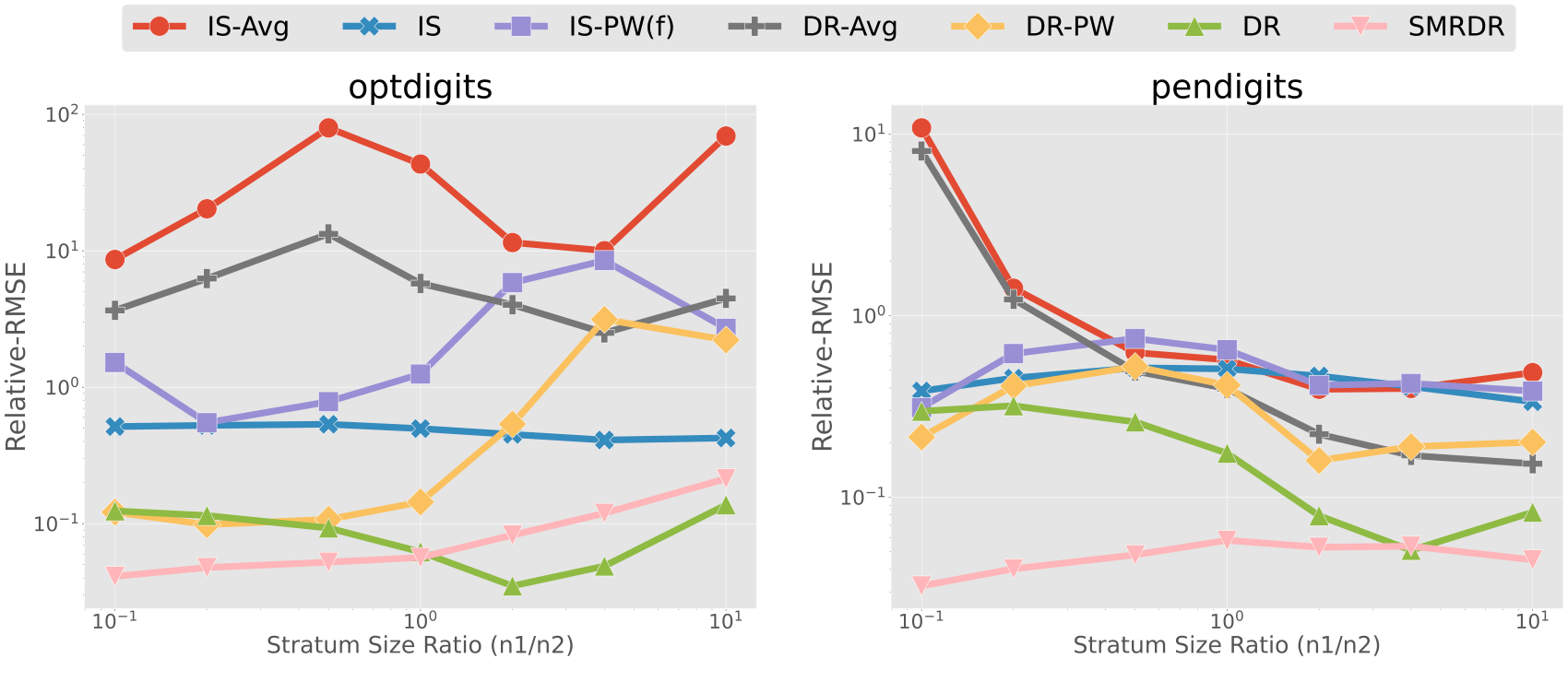
Fig. 2: Comparing proposed estimators to some variants of IS type estimators.

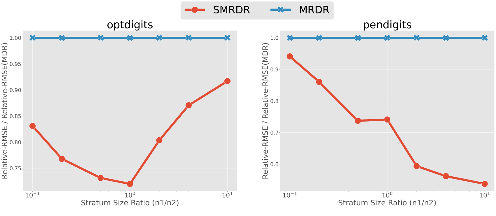
Fig. 3: Comparing SMRDR (leveraging the stratification) and MRDR (ignoring the stratification).

We split the original data into training (30%) and evaluation (70%) sets. We first obtain a deterministic policy $\pi_{\text{det}}$ by training a logistic regression model on the training set. Then, following Table 1, we construct evaluation and logging policies as mixtures of one of the deterministic policy and the uniform random policy $\pi_{u}$. We vary $\rho_{1}/(1-\rho_{1})=n_{1}/n_{2}$ in $\{0.1,0.25,0.5,1,2,4,10\}$. Since $\pi_{1}$ is closer to $\pi^{\mathrm{e}}$ than $\pi_{2}$, larger $\rho_{1}/\rho_{2}$ corresponds to an easier problem. We then split the evaluation dataset into two according to proportions $\rho_{1},\rho_{2}$ and in each dataset we use the corresponding policy to make decisions and generate reward observations (the true label is then omitted). Using the resulting dataset we consider various estimators $\hat{J}$ for $J$. We describe additional details of the experimental setup in Appendix E.

We repeat the process $M=200$ times with different random seeds and report the relative root MSE:

$$\text{Relative-RMSE}\ (\hat{J})=\frac{1}{J\sqrt{M}}\sqrt{\sum_{m=1}^{M}\left({J-\hat{J}_{m}}\right)^{2}}$$

where $\hat{J}_{m}$ is an estimated policy value with $m$-th data.

Table 1: The evaluation and logging policies used in the experiments.

evaluation policy ($\pi_{e}$)	$1.00\pi_{\text{det}}+0.00\pi_{u}$
logging policy 1 ($\pi_{1}$)	$0.95\pi_{\text{det}}+0.05\pi_{u}$
logging policy 2 ($\pi_{2}$)	$0.05\pi_{\text{det}}+0.95\pi_{u}$

Estimators considered.

We consider the following estimators:

• Our proposed estimators, $J_{\mathrm{DR}}\text{-$\hat{\pi}_{*}$},\hat{J}_{\text{SMRDR}}$.

• Standard estimators in the iid setting, $\hat{J}_{\text{IS}},\hat{J}_{\mathrm{MRDR}}$.

• (Feasible versions of) the two estimators proposed by (Agarwal et al., 2017), $\hat{J}_{\text{IS-Avg}},\hat{J}_{\text{IS-PW}}$.

• The natural doubly robust extension of these as discussed in Section 3.2, $\hat{J}_{\mathrm{DR}\text{-Avg}},\hat{J}_{\mathrm{DR}\text{-PW}}$.

We suppose we do not know logging policies. For all estimators, we estimate the logging policies using logistic regression on the evaluation set with 2-fold cross-fitting as in Algorithm 1. Most of the estimators above are introduced with known logging densities in the previous sections. Here, we just replace each $\pi_{k}$ with their estimates. For DR, DR-Avg, and DR-PW, we construct $q$-estimates using logistic regression again using 2-fold cross-fitting as in Algorithm 1. For SMRDR and MRDR, we optimize their respective estimated variance objectives over the class of logistic regression $\mathcal{Q}$. We use tensorflow and the same hyperparameter setting for DR, DR-Avg, DR-PW, SMRDR, and MRDR to ensure a fair comparison.

Results.

The resulting Relative-RMSEs on optdigits and pendigits datasets with varying values of $n_{1}/n_{2}$ are given in Figs. 3 and 3. Several findings emerge from the results. First, we see the dilemma pointed out by Agarwal et al. (2017): Specifically, the ordering of the variances of IS-Avg and IS-PW depend on the instance. More generally, there is no clear ordering between IS, IS-Avg, IS-PW, DR-Avg, and DR-PW. For example, on the optdigits data, DR-PW performs best among baselines with small values of $n_{1}/n_{2}$, while IS performs better with large values of $n_{1}/n_{2}$. This behavior is predicted by our analysis showing none of these estimators are optimal.

Second, our proposed estimators successfully resolve the dilemma and are superior to the above suboptimal estimators. Moreover, we see SMRDR generally performs better than DR, especially when overlap is weak ($n_{1}/n_{2}$ is small), which exacerbates issues of misspecification. It does appear that DR outperforms SMRDR in the specific example of optdigits when overlap is strong ($n_{1}/n_{2}$ is large), which might be attributed to bad optimization of the non-convex objective compared to a reasonably good-enough plug-in $q$-estimate.

Finally, we directly compare the performances of SMRDR and MRDR in Figure 3. We observe that SMRDR significantly outperforms MRDR in the stratified setting, leading to up to 45% reduction in error. This strongly highlights that even though the asymptotic efficiency bounds are the same in the stratified and iid settings, leveraging the stratification structure can still offer significant gains in the multiple logger setting.

8 Conclusions and Future Directions

We studied OPE in the multiple logger setting, framing it as a form of stratified sampling. We then studied optimality in several classes of estimators and showed that, at least asymptotically, the minimum MSE is the same among all of them. We proposed feasible estimators that can achieve this minimum, whether logging policies are known or not. This gives a concrete and positive resolution to the multiple logger dilemma posed in Agarwal et al. (2017). We further discuss how to take stratification into account when choosing best-in-class control variates.

There are a number of avenues for future work. One is to consider optimality in the case of adaptive data collection from multiple loggers, where each logger may depend on historical data so far (Luedtke and van der Laan, 2016; Hadad et al., 2019; Zhang et al., 2020; Kato et al., 2020). Another is to study off-policy optimization in the stratified setting, whether by policy search (Zhang et al., 2013; Kallus, 2018, 2017; He et al., 2019) or by off-policy gradient ascent (Kallus and Uehara, 2020b).

Appendix A Notation

We first summarize the notation we use in Table 2.

Table 2: Notation

$n,n_{k},\,(1\leq k\leq K),K$	Whole sample size, sample size, stratification size
$n^{\prime},n^{\prime}_{k},\,(1\leq k\leq K),K$	Sample size considering asymptotics
$\rho_{k}$	$n_{k}/n$
$J$	Policy value $\mathbb{E}_{\pi^{\mathrm{e}}}[r]$
$p_{S}(s),p_{R\mid S,A}(r\mid s,a)$	State, reward distributions
$s,a,r$	State, action, reward
$[K]$	Partition $[1,\cdots,K]$
$[Z]$	Partition for cross-fitting
$\mathcal{D}=\{\mathcal{D}_{1},\cdots,\mathcal{D}_{K}\},\mathcal{D}_{k}=\{S_{kj},A_{kj},R_{kj}\}_{j=1}^{K,n_{k}}$	Observed whole data, data in the size $k$
$\pi_{k},\pi_{*},\pi^{\mathrm{e}}$	$k$-th behavior policy, mixture of k policies, evaluation policy
$\mathbb{E}_{\pi}[f(k,s,a,r)],\mathrm{var}_{\pi}[f(k,s,a,r)]$	Expectation and variance regarding $\pi$
$\hat{J}_{\text{IS-Avg}},\hat{J}_{\text{IS}},\hat{J}_{\text{\text{IS-PW}}}$	Naïve IS, IS, precision-weighted IS estimator
$\hat{J}_{\mathrm{DR}},\hat{J}_{\text{SMRDR}}$	Doubly robust, Stratified more robust doubly robust estimator
$\{\Upsilon(\mathcal{D};\lambda)\},\{\Gamma(\mathcal{D};h,g)\}$	Set of some estimators
$\hat{J}_{\text{BI}}$	Feasible cross-fold version estimators
$\mathbb{E}_{n}[f(k,s,a,r)],\mathbb{E}_{n_{k}}[f(k,s,a,r)]$	Empirical approximation
$q(s,a),v(s)$	$\mathbb{E}[r|s,a],q(s,\pi^{\mathrm{e}})$
$\mathcal{N}(0,B)$	Normal distribution with mean $0$ and variance $B$
$\|f\|_{2}$	$\{\mathbb{E}_{\pi_{*}}[f^{2}(k,s,a,r)]\}^{1/2}$
$o$	$\{s_{jk},a_{jk},r_{jk}\}$
$\tilde{\phi}(o)$	EIF: $\frac{1}{n}\sum_{i=1}^{n}\left\{\frac{\pi^{\mathrm{e}}(a_{i}\mid s_{i})}{\pi_{*}(a_{i}\mid s_{i})}\{r_{i}-q(s_{i},a_{i})\}+q(s_{i},\pi^{\mathrm{e}})-J\right\}.$
$\phi(s,a,r;g)$	$\pi^{\mathrm{e}}/\pi\{r-g(s,a)\}+g(s,\pi^{\mathrm{e}})$
$\mathcal{Q}$	Function class for $g$ in $\{\phi(s,a,r;g)\}$ in SMRDR
$\mathcal{L}_{z},\mathcal{U}_{z}$	Set induced by sample splitting
$\sigma^{2}_{r}(s,a)$	Variance: $\mathrm{var}[r\mid s,a]$

Appendix B Off-policy Evaluation in Reinforcement Learning with Multiple Loggers

We discuss an efficiency bound and a method to achieve the efficiency bound when the data is generated by an MDP and multiple loggers.

Consider that we have a data $\mathcal{D}=\{D_{1},\cdots,D_{K}\}$:

$$\mathcal{D}_{k}=\{S_{kj},A_{kj},R_{kj},S^{\prime}_{kj}\}_{j=1}^{n_{k}}\overset{\text{i.i.d}}{\sim}p_{k}(s)\pi_{k}(a\mid s)p_{R\mid S,A}(r\mid s,a)p_{S^{\prime}|S,A}(s^{\prime}\mid s,a).$$

When $K=1$, this is a standard DGP assumption in an RL setting. Here, there are $K$-multiple loggers. State distribution $p_{k}(s)$ for each logger can be different as well as each behavior policy. We sometimes reindex the whole data as $\mathcal{D}=\{S_{i},A_{i},R_{i},S^{\prime}_{i}\}_{i=1}^{n}$. In this section, given some function $f(s,a,r,s^{\prime})$, we define

$$\mathbb{E}_{p_{k}(s)\times\pi_{k}}[f(s,a,r,s^{\prime})]:=\int f(s,a,r,s^{\prime})p_{k}(s)\pi_{k}(a\mid s)p_{R\mid S,A}(r\mid s,a)p_{S^{\prime}|S,A}(s^{\prime}\mid s,a)\mathrm{d}(s,a,r,s^{\prime}).$$

Our target is the policy value $J(\gamma)$ defined by the same MDP and an evaluation policy $\pi^{\mathrm{e}}$ with a discount factor $\gamma$ as follows:

$$J(\gamma)=(1-\gamma)\lim_{T\to\infty}\mathbb{E}[\sum_{t=1}^{T}\gamma^{t-1}r_{t}\mid s_{1}\sim p_{e}(s),a_{1}\sim\pi^{\mathrm{e}}(s_{1}),a_{2}\sim\pi^{\mathrm{e}}(s_{2}),\cdots],$$

where $p_{e}(s)$ is an initial state distribution. Here, we have an important observation

$$J(\gamma)=\mathbb{E}_{p^{(\infty)}_{e,\gamma}\times\pi^{\mathrm{e}}}[r],$$

where $p^{(\infty)}_{e,\gamma}(s)$ is an average visitation distribution with a discount factor $\gamma$ and an initial distribution $p_{e}(s)$. Based on Liu et al. (2018) when $K=1$, this is estimated by

$$\frac{1}{n}\sum_{i=1}^{n}\hat{w}(S_{i})\frac{\pi^{\mathrm{e}}(A_{i}\mid S_{i})}{\pi_{1}(A_{i}\mid S_{i})}R_{i}$$

where $\hat{w}(s)$ is some estimator for $w(s):=p^{(\infty)}_{e,\gamma}/p_{1}(s)$. In this $K=1$ setting, Kallus and Uehara (2019a) derived the efficiency bound and a way to achieve the efficiency bound.

Here, we give the efficiency bound with a multiple logger case. This is

$$\mathbb{E}_{\pi_{*}(s,a)}\left[\left\{\frac{p_{\pi^{\mathrm{e}},\gamma}(s)\pi^{\mathrm{e}}(a\mid s)}{\pi_{*}(s,a)}\right\}^{2}\mathrm{var}[r+\gamma q(s^{\prime},\pi^{\mathrm{e}})\mid s,a]\right],$$

where $\pi_{*}(s,a)=\sum_{k=1}^{K}(n_{k}/n)\pi_{k}(a\mid s)p_{k}(s)$. When $K=1$, this result is reduced to Kallus and Uehara (2019a). Though we do not give a formal derivation, this is derived in the same spirit of Theorem 4.

Next, we give an efficient estimator. Before that, we define $w(s,a):=\left\{\frac{p^{(\infty)}_{\pi^{\mathrm{e}},\gamma}(s)\pi^{\mathrm{e}}(a\mid s)}{\pi_{*}(s,a)}\right\}$, $q(s,a):=\mathbb{E}_{\pi^{\mathrm{e}}}[\sum_{t=1}^{\infty}\gamma^{t-1}r_{t}\mid s_{1}=s,a_{1}=a]$. The efficient estimator is

$$\frac{1}{n}\sum_{i=1}^{n}\hat{w}(S_{i},A_{i})\{R_{i}+\gamma\hat{q}(S^{\prime}_{i},\pi^{\mathrm{e}})-\hat{q}(S_{i},A_{i})\}+\mathbb{E}_{p_{e}(s)}[\hat{q}(s,\pi^{\mathrm{e}})]$$

given some estimators $\hat{w}(s,a),\hat{q}(s,a)$. Q-functions are estimated by any off-the-shelf methods such as fitted Q-iteration (Antos et al., 2008). We can estimate the ratio $w(s,a)$ using some methods agnostic to $p_{k}(s)$ and $\pi_{k}(a\mid s)$ following Uehara et al. (2020). More specifically, for some test function $f(s,a)$, this is estimated by solving

$$0=\frac{1}{n}\sum_{i=1}^{n}\left\{\gamma w(S_{i},A_{i};\beta)f(S^{\prime}_{i},\pi^{\mathrm{e}})-w(S_{i},A_{i};\beta)f(S_{i},A_{i})\right\}+(1-\gamma)\mathbb{E}_{p_{e}(s)}[f(s,\pi^{\mathrm{e}})],$$

w.r.t. $\beta$, where $w(s,a;\beta)$ is some model for $w(s,a)$. Here, $\pi_{*}$ is not included in the estimating equation. Note that this is different form the ones in Liu et al. (2018); Kallus and Uehara (2019a), which are not agnostic to $\pi_{k}(a\mid s)$.

Finally, note that our result is more sophisticated comparing to Chen et al. (2020) in the sense that (1) they consider a special case when $p_{k}(s)$ is a stationary distribution; however, our result is applied to any $p_{k}(s)$, (2) their estimator does not use a control variate; however, our estimator and optimality result take the control variate term $q(s,a)$ into account.

Appendix C Efficiency Bound

A central question is what is the smallest-possible error we can hope to achieve in estimating $J$. In parametric models, the Cramér-Rao lower bound gives the lower bound of the variance among unbiased estimators. We have a stronger result that the Cramér-Rao lower bound lower bounds the asymptotic MSE of all regular estimators (van der Vaart, 1998, Chapter 7). Besides, this Cramér-Rao lower bound is extended from parametric models to non or semiparametric models, which is called an efficiency bound (van der Vaart, 1998, Chaptre 25). Again, this efficiency bound lower bounds the asymptotic MSE of all regular estimators. Standard semiparametric theory is established under the i.i.d sampling (Bickel et al., 1998; Tsiatis, 2006). Since our data mechanism is not i.i.d (not identical though independent), it looks we cannot apply this theory.

Here, the trick to apply this theory to our setting is regarding a set of $n$ samples as one observation. In other words, we consider that we have $m$ copies of this single observation consisting of $n$ samples, where $n^{\prime}:=nm\to\infty$ with fixed $n$ as $m\to\infty$. We consider a nonparametric model $\mathcal{M}$:

$$p(o)=\prod_{k=1}^{K}\prod_{j=1}^{n_{k}}p_{S}(s_{kj})\pi_{k}(a_{kj}\mid s_{kj})p_{R\mid S,A}(r_{kj}\mid s_{kj},a_{kj}),$$

where each density is free except for the weak overlap constraint . We also consider another nonparametric model $\mathcal{M}_{b}$:

$$p(o)=\prod_{k=1}^{K}\prod_{j=1}^{n_{k}}p_{S}(s_{kj})\pi_{k}(a_{kj}\mid s_{kj})p_{R\mid S,A}(r_{kj}\mid s_{kj},a_{kj}),$$

where $\pi_{k}$ is fixed at the true value and other densities (state and reward densitiese) are free except for the weak overlap constraint. Then, the efficiency bound of each model lower bounds the limit of the MSE for any regular estimator $\hat{J}$ w.r.t each model.

To check this, we informally state this key property of the efficient influence function (EIF) in our setting.

Theorem 10.

Theorem 3 The EIF $\tilde{\phi}(o)$ is the gradient of $J$ w.r.t the model $\mathcal{M}$, which has the smallest $L_{2}$-norm and it satisfies that for any regular estimator $\hat{J}$ of J w.r.t the model $\mathcal{M}$, $\mathrm{AMSE}[\hat{J}]\geq\mathrm{var}[\phi(\mathcal{D})]$, where $\mathrm{AMSE}[\hat{J}]$ is the second moment of the limiting distribution of $\sqrt{n^{\prime}}(\hat{J}-J)$.

Note that a regular estimator is any whose limiting distribution is insensitive to small changes of order $\mathcal{O}(1/\sqrt{m})$ to the DGP in the model (van der Vaart, 1998, Chapter 7). This is a super broad class of estimators excluding pathological estimators such as Hodges’ estimator. The term $\mathrm{var}[\phi]$ is called the efficiency bound. For the current problem, the EIF and the efficiency bound are derived as follows.

Theorem 11.

Under the model $\mathcal{M}$, the EIF $\tilde{\phi}(o)$ is

$$\frac{1}{n}\sum_{i=1}^{n}\left\{\frac{\pi^{\mathrm{e}}(a_{i}\mid s_{i})}{\pi_{*}(a_{i}\mid s_{i})}\{r_{i}-q(s_{i},a_{i})\}+v(s_{i})-J\right\}.$$

The efficiency bound $V(\mathcal{M})$ scaled by $n$, i.e., $n\mathrm{var}[\tilde{\phi}(o)]$, is

$$\mathbb{E}_{\pi_{*}}\left[\left\{\frac{\pi^{\mathrm{e}}(a\mid s)}{\pi_{*}(a\mid s)}\right\}^{2}\mathrm{var}[r\mid s,a]\right]+\mathrm{var}_{p_{S}}[v(s)].$$

The EIF and efficiency bound are the same for the model $\mathcal{M}_{b}$.

We will give the formal proof in Appendix D. Before that, we show that this is exactly the Cramér-Rao lower bound in a finite, action, reward space setting.

Theorem 12.

Assume $\mathcal{S},\mathcal{A},\mathcal{R}$ is a finite space. Then, the Cramér-Rao lower bound of $J$ is $V(\mathcal{M}_{b})$.

Proof.

We define the Cramér-Rao lower bound of the target functional. Assume some parametric model

$$\{p_{S}(s;\theta_{0}),\pi_{1}(a\mid s;\theta_{1}),\cdots,\pi_{K}(a\mid s;\theta_{K}),p_{R|A,S}(r|a,s;\theta_{K+1})\},$$

where each parameter corresponds to each state, action and reward. For example, assume $\mathcal{S}=\{\mathfrak{S}_{1},\cdots,\mathfrak{S}_{b}\}$:

$$p_{S}(s;\theta_{0})=\left\{\sum_{i=1}^{b-1}I(\mathfrak{S}_{i}=s)\theta_{0i}\right\}-I(\mathfrak{S}_{b}=s)\theta_{0b}.$$

The $i$-th element of the score of this $p_{S}(s)$ ($1\leq i\leq b-1$) is

$$\log_{\theta_{0i}}p_{S}(s)=I(\mathfrak{S}_{i}=s)/\theta_{0i}-I(\mathfrak{S}_{b}=s)/\theta_{0b}.$$

Let us define a score function for a parametric submodel:

$$g_{S} =\nabla_{\theta_{0}}\log p_{S}(s;\theta_{0}),\,g_{k}=\nabla_{\theta_{k}}\log\pi_{k}(a\mid s;\theta_{k}),g_{R|A,S}=\nabla_{\theta_{K+1}}\log p_{R|A,S}(r|a,s;\theta_{K+1}),$$

$$g_{S,A,R} =\{g^{\top}_{S},g^{\top}_{1},\cdots,g^{\top}_{K},g^{\top}_{R|A,S}\}^{\top},\,g_{S,A}=\{g^{\top}_{1},\cdots,g^{\top}_{K}\}^{\top},\,\theta=\{\theta^{\top}_{0},\cdots,\theta^{\top}_{K+1}\}^{\top}.$$

The Cramér-Rao lower bound is defined as

$$\nabla_{\theta^{\top}}\mathbb{E}_{\pi^{\mathrm{e}}}[r]I(\theta)^{-1}\nabla_{\theta}\mathbb{E}_{\pi^{\mathrm{e}}}[r].$$

The term $I(\theta)$ is

$$I(\theta) =\sum_{k=1}^{K}\sum_{j=1}^{n_{k}}\begin{pmatrix}\mathbb{E}_{\pi_{k}}[\nabla_{\theta^{\top}_{0}}g_{S}]&\bm{0}&0\\ \bm{0}&\mathbb{E}_{\pi_{k}}[\nabla_{\theta^{\top}_{S,A}}g_{S,A}]&\bm{0}\\ 0&\bm{0}&\mathbb{E}_{\pi_{k}}[\nabla_{\theta^{\top}_{K+1}}g_{R|S,A}]\\ \end{pmatrix}$$

$$=n\begin{pmatrix}\mathbb{E}_{\pi_{*}}[\otimes g_{S}]&\bm{0}&0\\ \bm{0}&\frac{1}{n}\sum_{k=1}^{K}\sum_{j=1}^{n_{k}}\mathbb{E}_{\pi_{k}}[\nabla_{\theta^{\top}_{S,A}}g_{S,A}]&\bm{0}\\ 0&\bm{0}&\mathbb{E}_{\pi_{*}}[\otimes g_{R|S,A}]\\ \end{pmatrix}$$

In addition,

$$\nabla_{\theta}\mathbb{E}_{\pi^{\mathrm{e}}}[r]=(\mathbb{E}_{\pi^{\mathrm{e}}}[rg^{\top}_{S}],0,\cdots,0,\mathbb{E}_{\pi^{\mathrm{e}}}[rg^{\top}_{R|S,A}])^{\top}.$$

From matrix CS-inequality, this is transformed as

$$\nabla_{\theta^{\top}}\mathbb{E}_{\pi^{\mathrm{e}}}[r]I(\theta)^{-1}\nabla_{\theta}\mathbb{E}_{\pi^{\mathrm{e}}}[r]$$

$$=\frac{1}{n}\mathbb{E}_{\pi_{e}}[rg^{\top}_{R|A,S}]\mathbb{E}_{\pi_{*}}[g_{R|A,S}g_{R|A,S}^{\top}]^{-1}\mathbb{E}_{\pi_{e}}[g_{R|A,S}r]+\frac{1}{n}\mathbb{E}_{\pi_{e}}[rg^{\top}_{S}]\mathbb{E}_{\pi_{*}}[g_{S}g_{S}^{\top}]^{-1}\mathbb{E}_{\pi_{e}}[g_{S}r]$$

$$=\frac{1}{n}\mathbb{E}_{\pi_{*}}\left[\frac{\pi^{\mathrm{e}}}{\pi_{*}}\{r-q(s,a)\}g^{\top}_{R|A,S}\right]\mathbb{E}_{\pi_{*}}[g_{R|A,S}g_{R|A,S}^{\top}]^{-1}\mathbb{E}_{\pi_{*}}\left[\frac{\pi^{\mathrm{e}}}{\pi_{*}}\{r-q(s,a)\}g_{R|A,S}\right]$$

$$+\frac{1}{n}\mathbb{E}_{\pi_{*}}\left[(v(s)-J)g^{\top}_{S}\right]\mathbb{E}_{\pi_{*}}[g_{S}g_{S}^{\top}]^{-1}\mathbb{E}_{\pi_{*}}[g_{S}(v(s)-J)]$$

$$=\frac{1}{n}\mathbb{E}_{\pi_{*}}\left[\left\{\frac{\pi^{\mathrm{e}}}{\pi_{*}}(r-q(s,a))\right\}^{2}\right]+\frac{1}{n}\mathbb{E}_{\pi_{*}}[(v(s)-J)^{2}].$$

Here, we use the assumption that state, action and reward spaces are finite to state the last equality. For example, any function $g(s)$ s.t. $\mathbb{E}[g(s)]=0$ is represented as a linear combination of $\{\log_{\theta_{0i}}p_{S}(s)\}_{i=1}^{b-1}$. ∎

Appendix D Proof

Proof of Theorem 1.

We define $\mathbf{S}:=\{S_{kj}\},\mathbf{A}:=\{A_{kj}\}$. Then, by law of total variance, the variance of $\Gamma(\mathcal{D};h,g)$ is decomposed as follows:

$$\mathrm{var}\left[\frac{1}{n}\sum_{k=1}^{K}\sum_{j=1}^{n_{k}}h(k,S_{kj},A_{kj})\pi^{\mathrm{e}}(A_{kj}\mid S_{kj})\{R_{kj}-g(S_{kj},A_{kj})\}+g(S_{kj},\pi^{\mathrm{e}})\}\right]$$

$$=\mathbb{E}\left[\mathrm{var}\left[\frac{1}{n}\sum_{k=1}^{K}\sum_{j=1}^{n_{k}}h(k,S_{kj},A_{kj})\pi^{\mathrm{e}}(A_{kj}\mid S_{kj})\{R_{kj}-g(S_{kj},A_{kj})\}|\mathbf{S,A}\right]\right]$$

$$+\mathbb{E}\left[\mathrm{var}\left[\mathbb{E}\left[\frac{1}{n}\sum_{k=1}^{K}\sum_{j=1}^{n_{k}}h(k,S_{kj},A_{kj})\pi^{\mathrm{e}}(A_{kj}\mid S_{kj})\{R_{kj}-g(S_{kj},A_{kj})\}|\mathbf{S,A}\right]|\mathbf{S}\right]\right]$$

$$+\mathrm{var}\left[\mathbb{E}\left[\frac{1}{n}\sum_{k=1}^{K}\sum_{j=1}^{n_{k}}h(k,S_{kj},A_{kj})\pi^{\mathrm{e}}(A_{kj}\mid S_{kj})\{R_{kj}-g(S_{kj},A_{kj})\}+g(S_{kj},\pi^{\mathrm{e}})|\mathbf{S}\right]\right]$$ (5)

$$=\mathbb{E}\left[\mathrm{var}\left[\frac{1}{n}\sum_{k=1}^{K}\sum_{j=1}^{n_{k}}h(k,S_{kj},A_{kj})\pi^{\mathrm{e}}(A_{kj}\mid S_{kj})R_{kj}|\mathbf{S,A}\right]\right]$$ (6)

$$+\mathbb{E}\left[\mathrm{var}\left[\frac{1}{n}\sum_{k=1}^{K}\sum_{j=1}^{n_{k}}h(k,S_{kj},A_{kj})\pi^{\mathrm{e}}(A_{kj}\mid S_{kj})\{q(S_{kj},A_{kj})-g(S_{kj},A_{kj})\}|\mathbf{S,A}|\mathbf{S}\right]\right]+$$ (7)

$$+\mathrm{var}_{p_{S}(s)}\left[\frac{1}{n}q(s,\pi^{\mathrm{e}})\right].$$ (8)

The term (5) is converted into the term (8) because of the constraint (2). The term (7) takes $0$ when $g(s,a;p)=q(s,a)$. Thus, we only focus on the term (6). The term (6) is further expanded as

$$\frac{1}{n}\sum_{k=1}^{K}\rho_{k}\mathbb{E}_{\pi_{k}}[h^{2}(k,s,a)\{\pi^{\mathrm{e}}(a\mid s)\}^{2}\mathrm{var}[r\mid s,a]]=\frac{1}{n}\mathbb{E}_{\pi_{*}}\left[\sum_{k=1}^{K}\frac{\rho_{k}\pi_{k}(a\mid s)h^{2}(k,s,a)}{\pi_{*}}\{\pi^{\mathrm{e}}(a\mid s)\}^{2}\mathrm{var}[r\mid s,a]\right]$$

$$=\frac{1}{n}\mathbb{E}_{\pi_{*}}\left[\sum_{k=1}^{K}\frac{\rho^{2}_{k}\pi^{2}_{k}(a\mid s)h^{2}(k,s,a)}{\rho_{k}\pi_{k}\pi_{*}}\{\pi^{\mathrm{e}}(a\mid s)\}^{2}\mathrm{var}[r\mid s,a]\right]$$

$$\geq\frac{1}{n}\mathbb{E}_{\pi_{*}}\left[\frac{\{\sum_{k=1}^{K}\rho_{k}\pi_{k}(a\mid s)h(k,s,a)\}^{2}}{\pi^{2}_{*}(a\mid s)}\{\pi^{\mathrm{e}}(a\mid s)\}^{2}\mathrm{var}[r\mid s,a]\right]$$

$$=\frac{1}{n}\mathbb{E}_{\pi_{*}}\left[\frac{1}{\pi^{2}_{*}(a\mid s)}\{\pi^{\mathrm{e}}(a\mid s)\}^{2}\mathrm{var}[r\mid s,a]\right].$$

Here, we use CS-inequality in the second line. From the second line to the third line, we use the constraint (2):

$$\sum_{k=1}^{K}\rho_{k}\pi_{k}(a\mid s)h(k,s,a)=1.$$

This inequality becomes an equality when $h_{k}(s,a;p)=1/\pi_{*}$. In conclusion, we have

$$\mathrm{var}\left[\frac{1}{n}\sum_{k=1}^{K}\sum_{j=1}^{n_{k}}h(k,S_{kj},A_{kj})\pi^{\mathrm{e}}(A_{kj}\mid S_{kj})\{R_{kj}-g(S_{kj},A_{kj})\}+g(S_{kj},\pi^{\mathrm{e}})\right]$$

$$\geq\frac{1}{n}\mathbb{E}_{\pi_{*}}\left[\frac{1}{\pi^{2}_{*}(a\mid s)}\{\pi^{\mathrm{e}}(a\mid s)\}^{2}\mathrm{var}[r\mid s,a]\right]+\frac{1}{n}\mathrm{var}_{p_{S}}[v(s)].$$

and it becomes an equality when $g=q(s,a),h=1/\pi_{*}$.

Remark 1 (Another Proof).

This theorem is also proved from semiparametric theory in Appendix C.

Consider an estimator $\Gamma(\mathcal{D};h,g)$ by fixing $h$ and $g$ under $\mathcal{M}_{b}$. ($\mathcal{M}_{b}$ is the model where $\{\pi_{k}\}_{k=1}^{K}$ is known) Then, $\Gamma(\mathcal{D};h,g)$ is an asymptotically linear estimator. Thus, the influence function of an asymptotically linear estimator belongs to the set of gradients of $J$ relative to $\mathcal{M}_{b}$. The EIF has the smallest norm among this set of gradients. Thus,

$$\mathrm{var}[\Gamma(\mathcal{D};h,g)]\geq\mathrm{var}[\tilde{\phi}(\mathcal{D})].$$

∎

Proof of Theorem 2.

We consider the case $K=2$ for simplicity. We also suppose that samples in each strata are uniformly distributed. We prove

$$\hat{J}_{\text{BI}}(\hat{h},\hat{g}) =0.5\Gamma(\mathcal{L}_{1};\hat{g}^{(1)},\hat{h}^{(1)})+0.5\Gamma(\mathcal{L}_{2};\hat{g}^{(2)},\hat{h}^{(2)})$$ (9)

$$=0.5\Gamma(\mathcal{L}_{1};g,h)+0.5\Gamma(\mathcal{L}_{2};g,h)+\mathrm{o}_{p}(n^{-1/2}).$$ (10)

Then, the proof is immediately concluded from (stratified sampling) CLT. This is proved as follows.

The first term is further expanded as follows:

$$\Gamma(\mathcal{L}_{1};\hat{g}^{(1)},\hat{h}^{(1)}) =\{\Gamma(\mathcal{L}_{1};\hat{g}^{(1)},\hat{h}^{(1)})-\mathbb{E}[\Gamma(\mathcal{L}_{1};\hat{g}^{(1)},\hat{h}^{(1)})\mid\mathcal{U}_{1}]\}-\{\Gamma(\mathcal{L}_{1};g,h)-\mathbb{E}[\Gamma(\mathcal{L}_{1};g,h)]\}$$ (11)

$$+\mathbb{E}[\Gamma(\mathcal{L}_{1};\hat{g}^{(1)},\hat{h}^{(1)})\mid\mathcal{U}_{1}]-\mathbb{E}[\Gamma(\mathcal{L}_{1};g,h)]$$ (12)

$$+\Gamma(\mathcal{L}_{1};g,h).$$

First, (12) is $0$ since

$$\mathbb{E}[\Gamma(\mathcal{L}_{1};\hat{g}^{(1)},\hat{h}^{(1)})\mid\mathcal{U}_{1}]-\mathbb{E}[\Gamma(\mathcal{L}_{1};g,h)\mid\mathcal{U}_{1}]=J-J=0.$$

Here, we use the constraint (2) on $h$ and $\hat{h}$. Second, we show (11) is $\mathrm{o}_{p}(n^{\prime-1/2})$. The conditional expectation of (11) conditioning on $\mathcal{U}_{1}$ is $0$. The conditional variance conditioning on $\mathcal{U}_{1}$ is

$$\mathrm{var}\left[\Gamma(\mathcal{L}_{1};\hat{g}^{(1)},\hat{h}^{(1)})-\Gamma(\mathcal{L}_{1};g,h)\mid\mathcal{U}_{1}\right]$$

$$=\frac{1}{n^{\prime(1)}}\sum_{k=1}^{K}\rho_{k}\mathrm{var}_{\pi_{k}}[\hat{h}^{(1)}(k,s,a)\pi^{\mathrm{e}}(a\mid s)\{r-\hat{g}^{(1)}(s,a)\}+\hat{g}^{(1)}(s,\pi^{\mathrm{e}})-\{h(k,s,a)\pi^{\mathrm{e}}(a\mid s)\{r-g(s,a)\}\}-g(s,\pi^{\mathrm{e}})\mid\mathcal{U}_{1}].$$

We show that this term is $\mathrm{o}_{p}(n^{\prime-1})$. Then, the conditional Chebshev’s inequality concludes that (16) is $\mathrm{o}_{p}(n^{\prime-1/2})$. To see this, what we have to show is that $\mathrm{var}_{\pi_{k}}[\cdot]$ is $\mathrm{o}_{p}(1)$ in the above. In fact, we have

$$\mathrm{var}_{\pi_{k}}[\hat{h}^{(1)}(k,s,a)\pi^{\mathrm{e}}(a\mid s)\{r-\hat{g}^{(1)}(s,a)\}+\hat{g}^{(1)}(s,\pi^{\mathrm{e}})-\{h(k,s,a)\pi^{\mathrm{e}}(a\mid s)\{r-g(s,a)\}-g(s,\pi^{\mathrm{e}})\mid\mathcal{U}_{1}]$$

$$\leq 2\mathrm{var}_{\pi_{k}}[\{\hat{h}^{(1)}(k,s,a)-h(k,s,a)\}\pi^{\mathrm{e}}(a\mid s)r\mid\mathcal{U}_{1}]$$

$$+2\mathrm{var}_{\pi_{k}}[-h(k,s,a)\pi^{\mathrm{e}}(a\mid s)\hat{g}^{(1)}(s,a)+\hat{g}^{(1)}(s,\pi^{\mathrm{e}})+h_{k}(a,s)\pi^{\mathrm{e}}(a\mid s)g(s,a)-g(s,\pi^{\mathrm{e}})\mid\mathcal{U}_{1}]$$

$$+2\mathrm{var}_{\pi_{k}}[\{\hat{h}^{(1)}(k,s,a)-h(k,s,a)\}\pi^{\mathrm{e}}(a\mid s)\{\hat{g}^{(1)}(s,a)-g(s,a)\}\mid\mathcal{U}_{1}]$$

$$\lesssim\max(\|\hat{h}^{(1)}-h\|,\|\hat{g}^{(1)}-g\|)=\mathrm{o}_{p}(1).$$

Here, we use $\mathrm{var}_{\pi_{k}}[a+b]\leq 2\mathrm{var}_{\pi_{k}}[a]+2\mathrm{var}_{\pi_{k}}[b]$.

∎

Proof of Theorem 4.

Before checking this proof, refer to the proof of Theorem 5. We use the result there.

Since the model $\mathcal{M}_{b}$ is smaller than the model $\mathcal{M}$, the function $\tilde{\phi}(o)$ is still a gradient of $J$ w.r.t $\mathcal{M}_{b}$. We show this gradient again lies in the tangent space. First, we calculate the tangent space. The tangent space of the model $\mathcal{M}_{b}$ is

$$\left\{\sum_{k=1}^{K}\sum_{j=1}^{n_{k}}\left\{g_{0}(s_{kj})+g_{K+1}(s_{kj},a_{kj},r_{kj})\right\}\in L_{2}(o)\right\},$$

where

$$\mathbb{E}[g_{0}(S_{kj})]=0,\,\mathbb{E}[g_{K+1}(S_{kj},A_{kj},R_{kj})|S_{kj},A_{kj}]=0\,(1\leq k\leq K,1\leq j\leq n_{k}).$$

The function $\tilde{\phi}(o)$ lies in the tangent space by taking $g_{0}(s)=v(s),g_{K+1}(s,a,r)=(r-q(s,a))$.

∎

Proof of Theorem 5.

We follow the following steps.

1. Calculate some gradient (a candidate of EIF) of the target functional $J$ w.r.t model $\mathcal{M}$.

2. Calculate the tangent space w.r.t the model $\mathcal{M}$.

3. Show that a candidate of EIF in Step 1 lies in the tangent space. Then, this concludes that a candidate of EIF in Step 1 is actually the EIF.

Calculation of the gradient

We start with positing a parametric model:

$$p(o;\theta)=\prod_{k=1}^{K}\prod_{j=1}^{n_{k}}p_{S}(s_{kj};\theta_{0})\pi_{k}(a_{kj}\mid s_{kj};\theta_{k})p_{R\mid S,A}(r_{kj}\mid s_{kj},a_{kj};\theta_{K+1}).$$

We define the corresponding gradients:

$$g_{S}(s)=\nabla_{\theta_{0}}\log p_{S}(s),\,g(k,s,a)=\nabla_{\theta_{k}}\log\pi_{k}(a\mid s),\,g_{R\mid S,A}=\nabla_{\theta_{K+1}}\log p_{R\mid S,A}(r\mid s,a).$$

To derive some gradient of the target functional w.r.t $\mathcal{M}$, what we need is finding a function $f(o)$ satisfying

$$\nabla J(\theta)=\mathbb{E}[f(\mathcal{D})\nabla\log p(\mathcal{D};\theta)].$$

We take the gradient as follows:

$$\nabla J(\theta) =\mathbb{E}_{\pi_{*}}\left[\frac{\pi^{\mathrm{e}}}{\pi_{*}}r\left\{g_{S}(s)+g_{R\mid S,A}(s,a,r)\right\}\right]$$

$$=\mathbb{E}_{\pi_{*}}\left[\psi(s,a,r)\left\{g_{S}(s)+g_{R\mid S,A}(s,a,r)\right\}\right],$$

where $\psi(s,a,r)=\pi^{\mathrm{e}}/\pi_{*}(r-q(s,a))+v(s)-J$. This is equal to the following

$$\mathbb{E}\left[\left\{\frac{1}{n}\sum_{k=1}^{K}\sum_{j=1}^{n_{k}}\phi(S_{kj},A_{kj},R_{kj})\right\}\left\{\sum_{k=1}^{K}\sum_{j=1}^{n_{k}}g_{S}(S_{kj})+g_{k}(S_{kj},A_{kj})+g_{R|S.A}(S_{kj},A_{kj},R_{kj})\right\}\right]$$

since the above is equal to

$$\frac{1}{n}\sum_{k=1}^{K}n_{k}\mathbb{E}_{\pi_{k}}\left[\psi(s,a,r)\{g_{S}(s)+g_{k}(s,a)+g_{R\mid S,A}(s,a,r)\}\right]$$

$$=\frac{1}{n}\sum_{k=1}^{K}n_{k}\mathbb{E}_{\pi_{k}}\left[\psi(s,a,r)\{g_{S}(s)+g_{R\mid S,A}(s,a,r)\}\right]$$

$$=\mathbb{E}_{\pi_{*}}\left[\psi(s,a,r)\{g_{S}(s)+g_{R\mid S,A}(s,a,r)\}\right].$$

Thus, the following function

$$\tilde{\phi}(o)=\frac{1}{n}\sum_{k=1}^{K}\sum_{j=1}^{n_{k}}\psi(s_{kj},a_{kj},r_{kj}).$$

is a derivative of the target functional $J$ w.r.t the model $\mathcal{M}$.

Calculation of the tangent space

Following a standard derivation way of the tangent space. (Tsiatis, 2006; van der Vaart, 1998), the tangent space of the model $\mathcal{M}$ is

$$\left\{\sum_{k=1}^{K}\sum_{j=1}^{n_{k}}\left\{g_{0}(s_{kj})+g_{k}(s_{kj},a_{kj})+g_{K+1}(s_{kj},a_{kj},r_{kj})\right\}\in L_{2}(o)\right\}$$

where

$$\mathbb{E}[g_{0}(S_{kj})]=0,\mathbb{E}[g_{k}(S_{kj},A_{kj})|S_{kj}]=0,\,\mathbb{E}[g_{K+1}(S_{kj},A_{kj},R_{kj})|S_{kj},A_{kj}]=0\,(1\leq k\leq K,1\leq j\leq n_{k}).$$

and $L_{2}(o)$ is an $l_{2}$ space at the true density.

Last part

We can easily check that the $\tilde{\phi}(o)$ lies in the tangent space by taking $g_{0}(s)=v(s),g(k,s,a)=0,\,g_{K+1}(s,a,r)=(r-q(s,a))$. Thus, $\tilde{\phi}(o)$ is the EIF.

∎

Proof of Theorem 6.

In this proof, we define

$$\phi(s,a,r;\pi,g):=\pi^{\mathrm{e}}/\pi\{r-g\}+g(s,\pi^{\mathrm{e}}).$$

For simplicity, we consider the case where $K=2$ and assume that samples in each strata are uniformly distributed:

$$\hat{J}_{\mathrm{DR}}=0.5\mathbb{E}_{n^{\prime(1)}}[\phi(s,a,r;\hat{\pi}^{(1)}_{*},\hat{q}^{(1)})]+0.5\mathbb{E}_{n^{\prime(2)}}[\phi(s,a,r;\hat{\pi}^{(2)}_{*},\hat{q}^{(2)})],$$ (13)

where $\mathbb{E}_{{n^{\prime(i)}}}[\cdot]$ denotes an empirical approximation over the $i$-th fold data. We prove

$$\hat{J}_{\mathrm{DR}}=0.5\mathbb{E}_{n^{\prime(1)}}[\phi(s,a,r;\pi_{*},q)]+0.5\mathbb{E}_{n^{\prime(2)}}[\phi(s,a,r;\pi_{*},q)]+\mathrm{o}_{p}(n^{\prime-1/2}).$$ (14)

Then, the proof is immediately concluded from CLT.

The first term in Eq. 13 is further expanded as follows:

$$\mathbb{E}_{n^{\prime(1)}}[\phi(s,a,r;\hat{\pi}^{(1)}_{*},\hat{q}^{(1)})] =\frac{1}{\sqrt{n^{\prime(1)}}}\mathbb{G}_{n^{\prime(1)}}[\phi(s,a,r;\hat{\pi}^{(1)}_{*},\hat{q}^{(1)})-\phi(s,a,r;\pi_{*},q)]$$ (15)

$$-\mathbb{E}_{\pi_{*}}[\phi(s,a,r;\pi_{*},q)]+\mathbb{E}_{\pi_{*}}[\phi(s,a,r;\hat{\pi}^{(1)}_{*},\hat{q}^{(1)})\mid\mathcal{U}_{1}]$$ (16)

$$+\mathbb{E}_{n^{\prime(1)}}[\phi(s,a,r;\pi_{*},q)].$$

Here, we define

$$\frac{1}{\sqrt{n^{\prime(1)}}}\mathbb{G}_{n^{\prime(1)}}[\phi(s,a,r;\hat{\pi}^{(1)}_{*},\hat{q}^{(1)})-\phi(s,a,r;\pi_{*},q)]$$

$$=\left\{\mathbb{E}_{n^{\prime(1)}}[\phi(s,a,r;\hat{\pi}^{(1)}_{*},\hat{q}^{(1)})-\phi(s,a,r;\pi_{*},q)]-\mathbb{E}_{\pi_{*}}[\phi(s,a,r;\hat{\pi}^{(1)}_{*},\hat{q}^{(1)})-\phi(s,a,r;\pi_{*},q)\mid\mathcal{U}_{1}]\right\}$$

First, we show (16) is $\mathrm{o}_{p}(n^{\prime-1/2})$. This is proved as

$$\left|\mathbb{E}_{\pi_{*}}[\phi(s,a,r;\pi_{*},q)]-\mathbb{E}_{\pi_{*}}[\phi(s,a,r;\hat{\pi}^{(1)}_{*},\hat{q}^{(1)})\mid\mathcal{U}_{1}]\right|$$

$$=\left|\mathbb{E}_{\pi_{*}}\left[(\pi^{\mathrm{e}}/\pi_{*}-\pi^{\mathrm{e}}/\hat{\pi}^{(1)}_{*})(r-q)\mid\mathcal{U}_{1}\right]\right|+\left|\mathbb{E}_{\pi_{*}}\left[v-\hat{v}-\frac{\pi^{\mathrm{e}}}{\pi_{*}}q+\frac{\pi^{\mathrm{e}}}{\pi_{*}}\hat{q}\mid\mathcal{U}_{1}\right]\right|$$

$$+\left|\mathbb{E}_{\pi_{*}}\left[\{\pi^{\mathrm{e}}/\pi_{*}-\pi^{\mathrm{e}}/\hat{\pi}^{(1)}_{*}\}\{-q+q^{(1)}\}\mid\mathcal{U}_{1}\right]\right|$$

$$=|\mathbb{E}_{\pi_{*}}\left[\{\pi^{\mathrm{e}}/\pi_{*}-\pi^{\mathrm{e}}/\hat{\pi}^{(1)}_{*}\}\{-q+q^{(1)}\}\mid\mathcal{U}_{1}\right]|\lesssim\|\hat{\pi}^{(1)}_{*}-\pi_{*}\|_{2}\|\hat{q}^{(1)}-q\|_{2}=\mathrm{o}_{p}(n^{\prime-1/2}).$$

Second, we show (15) is $\mathrm{o}_{p}(n^{\prime-1/2})$. The conditional expectation conditioning on $\mathcal{U}_{1}$ is

$$\mathbb{E}\left[\left\{\mathbb{E}_{n^{\prime(1)}}[\phi(s,a,r;\hat{\pi}^{(1)}_{*},\hat{q}^{(1)})-\phi(s,a,r;\pi_{*},q)]\right\}\mid\mathcal{U}_{1}\right]-\mathbb{E}_{\pi_{*}}[\phi(s,a,r;\hat{\pi}^{(1)}_{*},\hat{q}^{(1)})-\phi(s,a,r;\pi_{*},q)\mid\mathcal{U}_{1}]$$

$$=0.$$

The conditional variance conditioning on $\mathcal{U}_{1}$ is

$$\mathrm{var}\left[\left\{\mathbb{E}_{n^{\prime(1)}}[\phi(s,a,r;\hat{\pi}^{(1)}_{*},\hat{q}^{(1)})-\phi(s,a,r;\pi_{*},q)]\right\}\mid\mathcal{U}_{1}\right]$$

$$=\frac{1}{n^{\prime(1)}}\sum_{k=1}^{K}\rho_{k}\mathrm{var}_{\pi_{k}}[\phi(s,a,r;\hat{\pi}^{(1)}_{*},\hat{q}^{(1)})-\phi(s,a,r;\pi_{*},q)\mid\mathcal{U}_{1}]$$

$$\leq\frac{1}{n^{\prime(1)}}\mathrm{var}_{\pi_{*}}[\phi(s,a,r;\hat{\pi}^{(1)}_{*},\hat{q}^{(1)})-\phi(s,a,r;\pi_{*},q)\mid\mathcal{U}_{1}]$$

$$\lesssim\frac{1}{n^{\prime(1)}}\max\{\|\hat{\pi}^{(1)}_{*}-\pi_{*}\|_{2},\,\|\hat{q}^{(1)}-q\|_{2}\}=\mathrm{o}_{p}(n^{\prime-1}).$$

From the second line to the third line, we invoke Theorem 8. Then, the conditional Chebshev’s inequality concludes that (15) is $\mathrm{o}_{p}(n^{\prime-1/2})$.

To summarize, (15) and (16) are $\mathrm{o}_{p}(n^{\prime-1/2})$. Thus, Eq. 14 is concluded.

∎

Proof of Theorem 7.

In this proof, we define

$$\phi(s,a,r;\pi,g):=\pi^{\mathrm{e}}/\pi\{r-g\}+g(s,\pi^{\mathrm{e}}).$$

For simplicity, we consider the case where $K=2$ and samples are uniformly distributed:

$$\hat{J}_{\mathrm{DR}}=0.5\mathbb{E}_{n^{\prime(1)}}[\phi(s,a,r;\hat{\pi}^{(1)}_{*},\hat{q}^{(1)})]+0.5\mathbb{E}_{n^{\prime(2)}}[\phi(s,a,r;\hat{\pi}^{(2)}_{*},\hat{q}^{(2)})].$$

where $\mathbb{E}_{{n^{\prime(i)}}}$ denotes an empirical approximation over the $i$-th fold data.

The first term is further expanded as follows:

$$\mathbb{E}_{n^{\prime(1)}}[\phi(s,a,r;\hat{\pi}^{(1)}_{*},\hat{q}^{(1)})]-J =\frac{1}{\sqrt{n^{\prime(1)}}}\mathbb{G}_{n^{\prime(1)}}[\phi(s,a,r;\hat{\pi}^{(1)}_{*},\hat{q}^{(1)})-\phi(s,a,r;\pi^{\dagger}_{*},q^{\dagger})]$$ (17)

$$-\mathbb{E}_{\pi_{*}}[\phi(s,a,r;\pi^{\dagger}_{*},q^{\dagger})]+\mathbb{E}_{\pi_{*}}[\phi(s,a,r;\hat{\pi}^{(1)}_{*},\hat{q}^{(1)})\mid\mathcal{U}_{1}]$$ (18)

$$+\mathbb{E}_{n^{\prime(1)}}[\phi(s,a,r;\pi^{\dagger}_{*},q^{\dagger})]-J.$$ (19)

As in the proof of Theorem 6, Eq. 17 is $\mathrm{o}_{p}(n^{\prime-1/2}_{1})$. The third term (19) is $\mathcal{O}_{p}(n^{\prime-1/2}_{1})$ from CLT noting the mean is $0$ because

$$\mathbb{E}[\mathbb{E}_{n^{\prime(1)}}[\phi(s,a,r;\pi^{\dagger}_{*},q^{\dagger})]]-J=0.$$

Here, we use the assumption that $\pi^{\dagger}_{*}$ or $q^{\dagger}$ is actually the true function. The second term is $\mathcal{O}_{p}(n^{\prime-1/2}_{1})$ since

$$|\mathbb{E}_{\pi_{*}}[\phi(s,a,r;\pi^{\dagger}_{*},q^{\dagger})]-\mathbb{E}_{\pi_{*}}[\phi(s,a,r;\hat{\pi}^{(1)}_{*},\hat{q}^{(1)})\mid\mathcal{U}_{1}]|$$

$$\leq\left|\mathbb{E}_{\pi_{*}}\left[(\pi^{\mathrm{e}}/\pi^{\dagger}_{*}-\pi^{\mathrm{e}}/\hat{\pi}^{(1)}_{*})(r-q^{\dagger})\mid\mathcal{U}_{1}\right]\right|+\left|\mathbb{E}_{\pi_{*}}\left[v^{\dagger}-\hat{v}-\frac{\pi^{\mathrm{e}}}{\pi_{*}}q^{\dagger}+\frac{\pi^{\mathrm{e}}}{\pi_{*}}\hat{q}\mid\mathcal{U}_{1}\right]\right|$$

$$+\left|\mathbb{E}_{\pi_{*}}\left[\{\pi^{\mathrm{e}}/\pi^{\dagger}_{*}-\pi^{\mathrm{e}}/\hat{\pi}^{(1)}_{*}\}\{-q^{\dagger}+q^{(1)}\}\mid\mathcal{U}_{1}\right]\right|$$

$$\lesssim\max(\|\hat{\pi}^{(1)}_{*}-\pi^{\dagger}_{*}\|_{2}\|,\hat{q}^{(1)}-q^{\dagger}\|_{2})=\mathcal{O}_{p}(n^{\prime-1/2}_{1}).$$

In conclusion, $\mathbb{E}_{n^{\prime(1)}}[\phi(s,a,r;\hat{\pi}^{(1)}_{*},\hat{q}^{(1)})]-J=\mathcal{O}_{p}(n^{\prime-1/2}_{1})$. This concludes that $\hat{J}_{\mathrm{DR}}$ is $\sqrt{n^{\prime}_{1}}$-consistent. ∎

Proof of Theorem 8.

Before stating the proof, in the DGP $\mathcal{D}^{\prime}$, we define $N_{i},(1\leq i\leq K)$:

$$(N_{1},\cdots,N_{K})\sim\mathrm{Multi}(n,\rho_{1},\cdots,\rho_{K}),$$

where $\mathbb{E}[N_{k}]=n_{k}$. Note that each $N_{i}$ is a random variable unlike a fixed constant $n_{i}$.

First, we show that this estimator is unbiased. This is proved as follows:

$$\mathbb{E}_{\pi_{*}}[\phi(s,a,r;g)]$$

$$=\int\phi(s,a,r;g)I(\pi_{*}(a\mid s)>0)p_{R\mid S,A}(r\mid s,a)\pi_{*}(a\mid s)p_{S}(s)\mathrm{d}(s,a,r)=J.$$

Next, we show the inequality $\mathrm{var}_{\mathcal{D}^{\prime}}[\mathbb{P}_{n}[\phi(s,a,r;g)]]\geq\mathrm{var}_{\mathcal{D}}[\mathbb{P}_{n}[\phi(s,a,r;g)]]$. From law of total variance, this is proved by

$$\mathrm{var}_{\mathcal{D}^{\prime}}[\mathbb{P}_{n}[\phi(s,a,r;g)]] =\mathbb{E}[\mathrm{var}_{D^{\prime}}[\mathbb{P}_{n}[\phi(s,a,r;g)]|\{N_{k}\}_{k=1}^{K}]]+\mathrm{var}[\mathbb{E}[\mathbb{P}_{n}[\phi(s,a,r;g)]|\{N_{k}\}_{k=1}^{K}|]]$$

$$\geq\mathbb{E}[\mathrm{var}_{D^{\prime}}[\mathbb{P}_{n}[\phi(s,a,r;g)]|\{N_{k}\}_{k=1}^{K}]]=\mathbb{E}\left[\frac{N_{k}}{n^{2}}\sum_{k=1}^{K}\mathrm{var}_{\pi_{k}}[\phi(s,a,r;g)]\right]$$

$$=\mathbb{E}\left[\frac{\rho_{k}}{n}\sum_{k=1}^{K}\mathrm{var}_{\pi_{k}}[\phi(s,a,r;g)]\right]=\mathrm{var}_{\mathcal{D}}[\mathbb{P}_{n}[\phi(s,a,r;g)]].$$

We show the last statement. First, we have

$$\mathbb{E}[\mathbb{P}_{n}[\phi(s,a,r;g)]|\{N_{k}\}_{k=1}^{K}|] =\frac{1}{n}\sum_{k=1}^{K}N_{k}\mathbb{E}_{\pi_{k}}\left[\frac{\pi^{\mathrm{e}}}{\pi_{*}}\{r-g(s,a)\}+g(s,\pi^{\mathrm{e}})\right]$$

$$=\mathbb{E}[g(s,\pi^{\mathrm{e}})]+\frac{1}{n}\sum_{k=1}^{K}N_{k}\mathbb{E}_{\pi_{k}}\left[\frac{\pi^{\mathrm{e}}}{\pi_{*}}\{r-g(s,a)\}\right].$$

Then, when $g(s,a)=q(s,a)$, the equality $\mathrm{var}_{\mathcal{D}^{\prime}}[\mathbb{P}_{n}[\phi(s,a,r;g)]]=\mathrm{var}_{\mathcal{D}}[\mathbb{P}_{n}[\phi(s,a,r;g)]]$ holds for any $\pi^{\mathrm{e}},\pi_{*}$ since

$$\mathrm{var}[\mathbb{E}[\mathbb{P}_{n}[\phi(s,a,r;g)]|\{N_{k}\}_{k=1}^{K}]]=0.$$

To get the equality $\mathrm{var}_{\mathcal{D}^{\prime}}[\mathbb{P}_{n}[\phi(s,a,r;g)]]=\mathrm{var}_{\mathcal{D}}[\mathbb{P}_{n}[\phi(s,a,r;g)]]$ for any $\pi^{\mathrm{e}},\pi_{*}$, we need

$$\mathbb{E}_{\pi_{k}}\left[\frac{\pi^{\mathrm{e}}}{\pi_{*}}\{r-g(s,a)\}\right]=0,\,\forall\pi_{*},\pi^{\mathrm{e}},1\leq\forall k\leq K.$$

This implies

$$\mathbb{E}_{\pi_{*}}[\pi^{\mathrm{e}}/\pi_{*}\{r-g(s,a)\}]=\mathbb{E}_{\pi^{\mathrm{e}}}[q(s,a)-g(s,a)]=0,\forall\pi^{\mathrm{e}},\pi_{*}.$$

This is only satisfied when $q(s,a)=g(s,a)$.

Remark 2.

We can show the statement of the inequality regarding the variances by more direct calculation. We have

$$\mathrm{var}_{\pi_{*}}\left[\phi(s,a,r;g)\right] =\mathbb{E}_{\pi_{*}}\left[\left\{\phi(s,a,r;g)\right\}^{2}\right]-\mathbb{E}_{\pi^{\mathrm{e}}}[r]^{2},$$

$$\sum_{k=1}^{K}\frac{n_{k}}{n}\mathrm{var}_{\pi_{k}}\left[\phi(s,a,r;g)\right] =\mathbb{E}_{\pi_{*}}\left[\left\{\phi(s,a,r;g)\right\}^{2}\right]-\sum_{k=1}^{K}\frac{n_{k}}{n}\mathbb{E}_{\pi_{k}}\left[\phi(s,a,r;g)\right]^{2}.$$

Thus, the desired statement $\mathrm{var}_{\mathcal{D}^{\prime}}[\mathbb{P}_{n}[\phi(s,a,r;g)]]\geq\mathrm{var}_{\mathcal{D}}[\mathbb{P}_{n}[\phi(s,a,r;g)]]$ for any $\pi^{\mathrm{e}},\pi_{*}$ is reduced to

$$\mathbb{E}_{\pi^{\mathrm{e}}}[r]^{2}\leq\sum_{k=1}^{K}\frac{n_{k}}{n}\mathbb{E}_{\pi_{k}}\left[\phi(s,a,r;g)\right]^{2}.$$

This is proved by

$$\mathbb{E}_{\pi^{\mathrm{e}}}\left[r\right]^{2} =\left\{\sum_{k=1}^{K}\frac{n_{k}}{n}\mathbb{E}_{\pi_{k}}\left[\phi(s,a,r;g)\right]\right\}^{2}=\sum_{k=1,j=1}^{K}\frac{n_{k}n_{j}}{n^{2}}\mathbb{E}_{\pi_{k}}\left[\phi(s,a,r;g)\right]\mathbb{E}_{\pi_{j}}\left[\phi(s,a,r;g)\right]$$

$$\leq\sum_{k=1,j=1}^{K}\frac{n_{k}n_{j}}{2n^{2}}\left\{\mathbb{E}_{\pi_{k}}\left[\phi(s,a,r;g)\right]^{2}+\mathbb{E}_{\pi_{j}}\left[\phi(s,a,r;g)\right]^{2}\right\}=\sum_{k=1}^{K}\frac{n_{k}}{n}\mathbb{E}_{\pi_{k}}\left[\phi(s,a,r;g)\right]^{2}.$$

Here, we use $2ab\leq a^{2}+b^{2}$.

∎

Proof of Theorem 9.

From the assumption, we have $\|\hat{q}^{(1)}_{\text{SMRDR}}-\check{q}\|=\mathrm{o}_{p}(1)$. We consider the case $K=2$ for simplicity:

$$\hat{J}_{\text{SMRDR}}=0.5\mathbb{E}_{n^{\prime(1)}}[\phi(s,a,r;\hat{q}^{(1)}_{\text{SMRDR}})]+0.5\mathbb{E}_{n^{\prime(2)}}[\phi(s,a,r;\hat{q}^{(2)}_{\text{SMRDR}})].$$

where $\mathbb{E}_{{n^{\prime(i)}}}$ denotes an empirical approximation over the $i$-th fold data. The first term is further expanded as follows:

$$\mathbb{E}_{n^{\prime(1)}}[\phi(s,a,r;\hat{q}^{(1)}_{\text{SMRDR}})]-J =\frac{1}{\sqrt{n^{\prime(1)}}}\mathbb{G}_{n^{\prime(1)}}[\phi(s,a,r;\hat{q}^{(1)}_{\text{SMRDR}})-\phi(s,a,r;\check{q})]$$ (20)

$$-\mathbb{E}_{\pi_{*}}[\phi(s,a,r;\check{q})]+\mathbb{E}_{\pi_{*}}[\phi(s,a,r;\hat{q}^{(1)}_{\text{SMRDR}})\mid\mathcal{U}_{1}]$$ (21)

$$+\mathbb{E}_{n^{\prime(1)}}[\phi(s,a,r;\check{q})]-J.$$ (22)

As in the proof of Theorem 6, Eq. 20 is $\mathrm{o}_{p}(n^{\prime-1/2}_{1})$. The second term is $0$. In conclusion,

$$\mathbb{E}_{n^{\prime(1)}}[\phi(s,a,r;\hat{q}^{(1)}_{\text{SMRDR}})]-J=\mathbb{E}_{n^{\prime(1)}}[\phi(s,a,r;\check{q})]-J+o_{p}(n^{\prime-1/2}_{1}).$$

This concludes the statement:

$$\hat{J}_{\text{SMRDR}}-J=\mathbb{E}_{n}[\phi(s,a,r;\check{q})]-J+o_{p}(n^{\prime-1/2}_{1}).$$

∎

Table 3: Dataset Statistics

Dataset Name	OptDigits	SatImage	PenDigits	Letter
#Classes ($l$)	10	6	10	26
#Data ($n$)	5620	6435	10992	20000

Appendix E Detailed Experimental Setup and Additional Results

Datasets.

We use 4 datasets from the UCI Machine Learning Repository. The dataset statistics are displayed in Table 3.

Detailed Experimental Procedure.

A multi-class classification dataset consists of $(s_{i},y_{i})_{i=1}^{n}$ where $s_{i}\in\mathbb{R}^{d}$ is a context vector and $y_{i}\in\{1,\cdots,l\}$ is a class for an index $i$. The value $l$ is the number of class. A classification algorithm assigning $s$ to $y$ is considered to be a policy from a context to an action where we regard $y$ as an action. When the prediction by the algorithm is correct, i.e., $y_{i}=\hat{y}_{i}$, we observe the unit reward $i$, otherwise the reward is $0$. In this way, we can construct a contextual bandit dataset consisting of the set of triplets $\{(s_{i},a_{i},r_{i})\}_{i=1}^{n}$ where $a_{i}:=\hat{y}_{i}$ and $r_{i}:=\mathbb{I}\{y_{i}=\hat{y}_{i}\}$.

We summarize the whole experimental procedures below:

1. We split the original data into training (30%) and evaluation (70%) sets.

2. We train logistic regression using the training set to obtain a base deterministic policy $\pi_{\text{det}}$.

3. Following Table 1, we construct the logging and evaluation policies.

4. We measure the accuracy of the evaluation policy and use it as its ground truth policy value.

5. We regard $100\times\rho_{1}/(1-\rho_{1})=n_{1}/n_{2}$% of the evaluation set as $\mathcal{D}_{1}$ (generated by $\pi_{1}$) and the rest as $\mathcal{D}_{2}$ (generated by $\pi_{2}$) where $\rho_{1}/(1-\rho_{1})=n_{1}/n_{2}\in\{0.1,0.25,0.5,1,2,4,10\}$. A smaller value of $n_{1}/n_{2}$ leads to a larger data size of $\mathcal{D}_{2}$ that is generated by a logging policy dissimilar to the evaluation policy.

6. Using the evaluation set (consisting of $\mathcal{D}_{1}$ and $\mathcal{D}_{2}$), an estimator $\hat{J}$ estimates the policy value of the evaluation policy $J$.

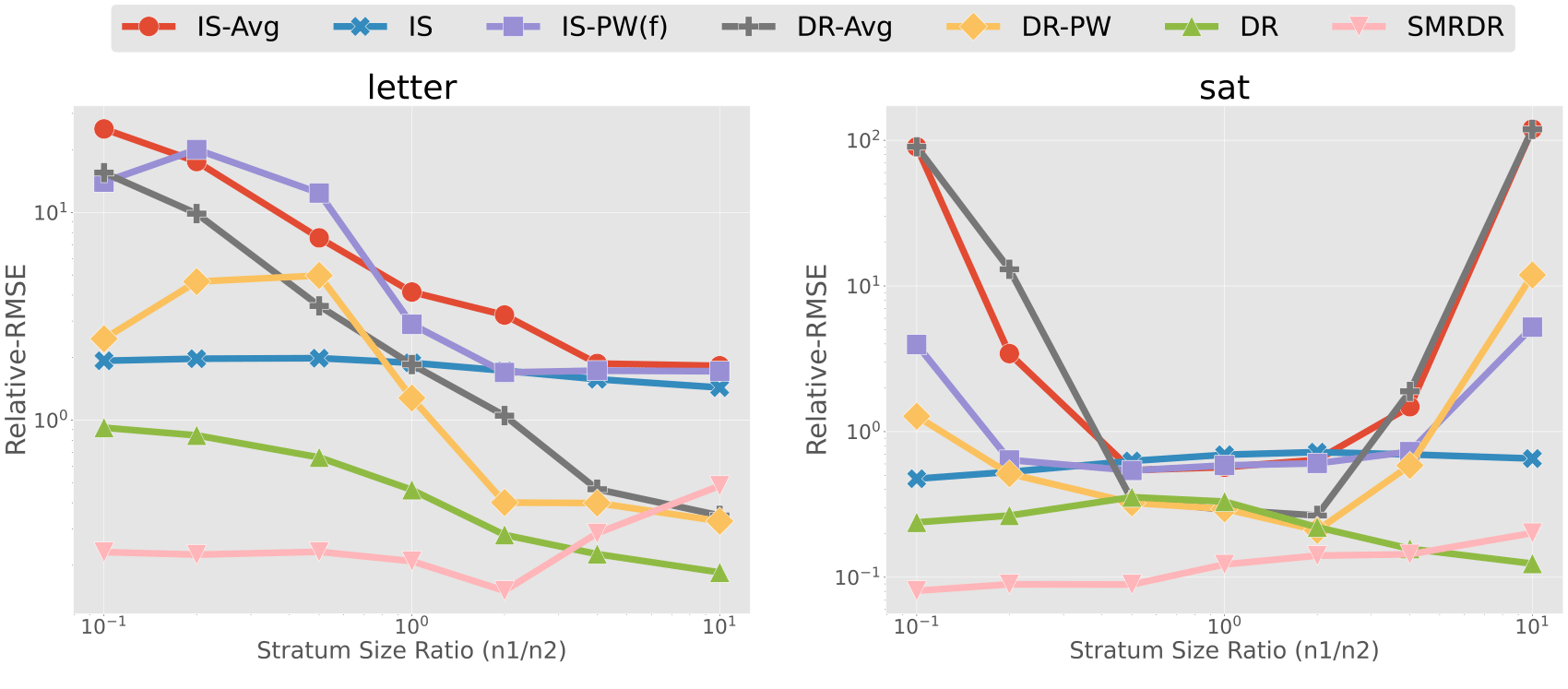
Fig. 4: Comparing proposed estimators to some variants of IS type estimators.

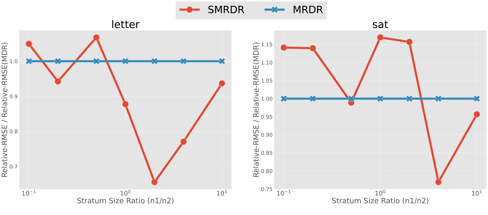
Fig. 5: Comparing SMRDR (leveraging the stratification) and MRDR (ignoring the stratification).

Additional Results.

Figure 5 and 5 show the results on the same experiment as conducted in Section 7 in the main text on the SatImage and Letter datasets.

References

• Agarwal et al. (2017) Agarwal, A., S. Basu, T. Schnabel, and T. Joachims (2017). Effective evaluation using logged bandit feedback from multiple loggers. KDD ’17, pp.  687–696.
• Antos et al. (2008) Antos, A., C. Szepesvári, and R. Munos (2008). Learning near-optimal policies with bellman-residual minimization based fitted policy iteration and a single sample path. Machine Learning 71, 89–129.
• Bareinboim and Pearl (2016) Bareinboim, E. and J. Pearl (2016). Causal inference and the data-fusion problem. Proceedings of the National Academy of Sciences.
• Bickel et al. (1998) Bickel, P. J., C. A. J. Klaassen, Y. Ritov, and J. A. Wellner (1998). Efficient and Adaptive Estimation for Semiparametric Models. Springer.
• Cao et al. (2009) Cao, W., A. A. Tsiatis, and M. Davidian (2009). Improving efficiency and robustness of the doubly robust estimator for a population mean with incomplete data. Biometrika 96, 723–734.
• Chen et al. (2020) Chen, X., L. Wang, Y. Hang, H. Ge, and H. Zha (2020). Infinite-horizon off-policy policy evaluation with multiple behavior policies. In Proceedings of the 8th International Conference on Learning Representations (ICLR), 2020.
• Chernozhukov et al. (2018) Chernozhukov, V., D. Chetverikov, M. Demirer, E. Duflo, C. Hansen, W. Newey, and J. Robins (2018). Double/debiased machine learning for treatment and structural parameters. Econometrics Journal 21, C1–C68.
• Dudík et al. (2014) Dudík, M., D. Erhan, J. Langford, L. Li, et al. (2014). Doubly robust policy evaluation and optimization. Statistical Science 29(4), 485–511.
• Farajtabar et al. (2018) Farajtabar, M., Y. Chow, and M. Ghavamzadeh (2018). More robust doubly robust off-policy evaluation. In Proceedings of the 35th International Conference on Machine Learning, 1447–1456.
• Geyer (1994) Geyer, C. J. (1994). Estimating normalizing constants and reweighting mixtures in markov chain monte carlo. Technical Report 568. School of Statistics, University of Minnesota, Minneapolis.
• Gutmann and Hyvärinen (2010) Gutmann, M. and A. Hyvärinen (2010). Noise-contrastive estimation: A new estimation principle for unnormalized statistical models. Volume 9 of Proceedings of Machine Learning Research, pp. 297–304.
• Hadad et al. (2019) Hadad, V., D. A. Hirshberg, R. Zhan, S. Wager, and S. Athey (2019). Confidence intervals for policy evaluation in adaptive experiments. arXiv preprint arXiv:1911.02768.
• He et al. (2019) He, L., L. Xia, W. Zeng, Z.-M. Ma, Y. Zhao, and D. Yin (2019). Off-policy learning for multiple loggers. In Proceedings of the 25th ACM SIGKDD International Conference on Knowledge Discovery & Data Mining.
• Jiang and Li (2016) Jiang, N. and L. Li (2016). Doubly robust off-policy value evaluation for reinforcement learning. In Proceedings of the 33rd International Conference on International Conference on Machine Learning-Volume, 652–661.
• Kallus (2017) Kallus, N. (2017). Recursive partitioning for personalization using observational data. In International Conference on Machine Learning, pp. 1789–1798. PMLR.
• Kallus (2018) Kallus, N. (2018). Balanced policy evaluation and learning. In Advances in Neural Information Processing Systems, pp. 8895–8906.
• Kallus and Uehara (2019a) Kallus, N. and M. Uehara (2019a). Efficiently breaking the curse of horizon: Double reinforcement learning in infinite-horizon processes. arXiv preprint arXiv:1909.05850.
• Kallus and Uehara (2019b) Kallus, N. and M. Uehara (2019b). Intrinsically efficient, stable, and bounded off-policy evaluation for reinforcement learning. In Advances in Neural Information Processing Systems 32, pp. 3320–3329.
• Kallus and Uehara (2020a) Kallus, N. and M. Uehara (2020a). Double reinforcement learning for efficient off-policy evaluation in markov decision processes. Journal of Machine Learning Research 21, 1–63.
• Kallus and Uehara (2020b) Kallus, N. and M. Uehara (2020b). Statistically efficient off-policy policy gradients. ICML 2020 (To appear).
• Kato et al. (2020) Kato, M., T. Ishihara, J. Honda, and Y. Narita (2020). Adaptive experimental design for efficient treatment effect estimation. arXiv preprint arXiv: 2002.05308.
• Kong et al. (2003) Kong, A., P. McCullagh, X. L. Meng, D. Nicolae, and Z. Tan (2003). A theory of statistical models for monte carlo integration. Journal of the Royal Statistical Society. Series B, Statistical methodology 65(3), 585–618.
• Liu et al. (2018) Liu, Q., L. Li, Z. Tang, and D. Zhou (2018). Breaking the curse of horizon: Infinite-horizon off-policy estimation. In Advances in Neural Information Processing Systems 31, pp. 5356–5366.
• Luedtke and van der Laan (2016) Luedtke, A. R. and M. J. van der Laan (2016, 04). Statistical inference for the mean outcome under a possibly non-unique optimal treatment strategy. Ann. Statist. 44(2), 713–742.
• Mandel et al. (2014) Mandel, T., Y. Liu, S. Levine, E. Brunskill, and Z. Popovic (2014). Off-policy evaluation across representations with applications to educational games. In Proceedings of the 13th International Conference on Autonomous Agentsand Multi-agent Systems, 1077–1084.
• Muandet et al. (2020) Muandet, K., M. Kanagawa, S. Saengkyongam, and S. Marukatat (2020). Counterfactual mean embeddings. Journal of Machine Learning Research (To appear).
• Munos et al. (2016) Munos, R., T. Stepleton, A. Harutyunyan, and M. Bellemare (2016). Safe and efficient off-policy reinforcement learning. In Advances in Neural Information Processing Systems 29, pp. 1054–1062.
• Murphy (2003) Murphy, S. A. (2003). Optimal dynamic treatment regimes. Journal of the Royal Statistical Society: Series B (Statistical Methodology) 65, 331–355.
• Narita et al. (2019) Narita, Y., S. Yasui, and K. Yata (2019). Efficient counterfactual learning from bandit feedback. AAAI.
• Rubin and der Laan (2008) Rubin, D. B. and M. J. V. der Laan (2008). Empirical efficiency maximization: Improved locally efficient covariate adjustment in randmized experiments and survival analysis. International Journal of Biostatistics 4, Article 5.
• Strehl et al. (2010) Strehl, A. L., J. Langford, L. Li, and S. M. Kakade (2010). Learning from Logged Implicit Exploration Data. In Proceedings of the 23rd International Conference on Neural Information Processing Systems, pp.  2217–2225.
• Su et al. (2020) Su, Y., P. Srinath, and A. Krishnamurthy (2020). Adaptive estimator selection for off-policy evaluation. arXiv preprint arXiv:2002.07729.
• Swaminathan et al. (2017) Swaminathan, A., A. Krishnamurthy, A. Agarwal, M. Dudik, J. Langford, D. Jose, and I. Zitouni (2017). Off-policy evaluation for slate recommendation. In Advances in Neural Information Processing Systems 30, pp. 3632–3642.
• Tan (2004) Tan, Z. (2004). On a likelihood approach for monte carlo integration. Journal of the American Statistical Association 99(468), 1027–1036.
• Thomas and Brunskill (2016) Thomas, P. and E. Brunskill (2016). Data-efficient off-policy policy evaluation for reinforcement learning. In Proceedings of the 33rd International Conference on Machine Learning, 2139–2148.
• Tsiatis (2006) Tsiatis, A. A. (2006). Semiparametric Theory and Missing Data. Springer Series in Statistics. New York, NY: Springer New York.
• Uehara et al. (2020) Uehara, M., J. Huang, and N. Jiang (2020). Minimax weight and q-function learning for off-policy evaluation. ICML 2020 (To appear).
• Uehara et al. (2018) Uehara, M., T. Matsuda, and H. Komaki (2018). Analysis of noise contrastive estimation from the perspective of asymptotic variance. arXiv preprint arXiv:1808.07983.
• van der Vaart (1998) van der Vaart, A. W. (1998). Asymptotic statistics. Cambridge, UK: Cambridge University Press.
• Wang et al. (2017) Wang, Y.-X., A. Agarwal, and M. Dudik (2017). Optimal and adaptive off-policy evaluation in contextual bandits. In Proceedings of the 34th International Conference on Machine Learning, pp.  3589–3597.
• Wooldridge (2001) Wooldridge, J. M. (2001). Asymptotic properties of weighted m -estimators for standard stratified samples. Econometric Theory 17, 451–470.
• Yin et al. (2020) Yin, M., Y. Bai, and Y.-X. Wang (2020). Near optimal provable uniform convergence in off-policy evaluation for reinforcement learning.
• Zhang et al. (2013) Zhang, B., A. A. Tsiatis, E. B. Laber, and M. Davidian (2013). Robust estimation of optimal dynamic treatment regimes for sequential treatment decisions. Biometrika 100, 681–694.
• Zhang et al. (2020) Zhang, K. W., L. Janson, and S. A. Murphy (2020). Inference for batched bandits. arXiv preprint arXiv:2002.03217.
• Zheng and van Der Laan (2011) Zheng, W. and M. J. van Der Laan (2011). Cross-validated targeted minimum-loss-based estimation. In Targeted Learning: Causal Inference for Observational and Experimental Data, Springer Series in Statistics, pp.  459–474. New York, NY: Springer New York.