Balance Maximization in Signed Networks via Edge Deletions

Abstract.

In signed networks, each edge is labeled as either positive or negative. The edge sign captures the polarity of a relationship. Balance of signed networks is a well-studied property in graph theory. In a balanced (sub)graph, the vertices can be partitioned into two subsets with negative edges present only across the partitions. Balanced portions of a graph have been shown to increase coherence among its members and lead to better performance. While existing works have focused primarily on finding the largest balanced subgraph inside a graph, we study the network design problem of maximizing balance of a target community (subgraph). In particular, given a budget $b$ and a community of interest within the signed network, we aim to make the community as close to being balanced as possible by deleting up to $b$ edges. Besides establishing NP-hardness, we also show that the problem is non-monotone and non-submodular. To overcome these computational challenges, we propose heuristics based on the spectral relation of balance with the Laplacian spectrum of the network. Since the spectral approach lacks approximation guarantees, we further design a greedy algorithm, and its randomized version, with provable bounds on the approximation quality. The bounds are derived by exploiting pseudo-submodularity of the balance maximization function. Empirical evaluation on eight real-world signed networks establishes that the proposed algorithms are effective, efficient, and scalable to graphs with millions of edges.

1. Introduction and Related Work

Graphs can model various complex systems such as knowledge graphs (Paulheim, 2017), road networks (Medya et al., 2018b), communication networks (Mitra et al., 2015), and social networks (Kempe et al., 2003). Typically, nodes represent entities, and edges characterize relationships between pairs of entities. Signed graphs further enhance the representative power of graphs by capturing the polarity of a relationship through positive and negative edge labels (Harary et al., 1953; Hüffner et al., 2007; Ordozgoiti et al., 2020). For example, if a graph represents social interactions, a positive edge would denote friendly interaction, and a negative edge would indicate a hostile relationship. Similarly, in a collaboration network, positive edges may indicate complementary skill sets, whereas negative edges would indicate disparate skills.

Signed graphs were first studied by Harary et al. (Harary et al., 1953) with particular focus on their balance. A balanced signed graph is one in which the vertices can be partitioned into two sets such that all edges inside each partition have a positive sign and all the negative signed edges are across the partitions. Balance is correlated with both positive and negative side-effects on a community. On the positive side, balanced communities are positively correlated with performance in financial networks where edges represent trading links (Askarisichani et al., 2019; Figueiredo and Frota, 2014). On the negative side, in social networks, balanced communities often promote “echo-chambers”, reduce diversity of opinions, and ultimately lead to more polarized viewpoints (Garimella and Weber, 2017).

Owing to the correlation of balance with several higher-order functional traits, it is natural to measure how far a community is from being balanced. For example, in financial networks, it is important to evaluate how the community may be engineered to further improve its balance. On the other hand, in social networks, an adversary, such as a political party, may be interested in polarizing the community in its favor by further increasing its balance. To avoid such adversarial attacks, it is important to know the weak links in a community so that they can be safeguarded.

In this paper, we address these applications by studying the problem of maximizing balance via edge deletions (Mbed). In the Mbed problem, we are given a graph, a target community within this graph, and a budget $b$. Our goal is to remove $b$ edges, such that the community gets as close to being balanced as possible. We formally define the notion of balance closeness in § 2. Deleting an edge would correspond to actions such as unfollowing or blocking a connection. If increasing balance is desirable, then Mbed provides a mechanism towards achieving the goal. On the other hand, Mbed also measures how susceptible a community is to adversarial attacks by revealing how much the balance can be increased through a small number of deletions, and which are these critical edges that must be protected.

1.1. Related Work

The problem we study falls in the class of network design problems. In network design, the goal is to modify the network so that an objective function modeling a desirable property is optimized. Examples of such objective functions include optimizing shortest path distances (traffic and sustainability improvement) (Meyerson and Tagiku, 2009; Dilkina et al., 2011; Lin and Mouratidis, 2015; Medya et al., 2018b), increasing centrality of target nodes by adding a small set of edges (Crescenzi et al., 2015; Ishakian et al., 2012; Medya et al., 2018a), optimizing the $k$-core(Medya et al., 2020; Zhou et al., 2019), manipulating node similarities (Dey and Medya, 2020), and boosting/containing influence on social networks (Kimura et al., 2008; Chaoji et al., 2012; Medya et al., 2020).

While several works exist on finding balanced subgraphs (Harary et al., 1953; Figueiredo and Frota, 2014; DasGupta et al., 2007; Hüffner et al., 2007; Ordozgoiti et al., 2020), work on optimizing balance through network design is rather limited. The only work is by Akiyama et al. (Akiyama et al., 1981), where they study the minimum number of sign flips needed to make a graph balanced. However our work is different for several reasons. First, (Akiyama et al., 1981) does not have any notion of a budget constraint. Second, the cascading impact of a sign flip and an edge deletion on the balance of a graph is significantly different. Third, (Akiyama et al., 1981) lacks evaluation on large real world graphs containing millions of edges. Finally, from a practicality viewpoint, selectively flipping the sign of an edge is difficult since the edge sign encodes the nature of interaction between the two entities (endpoints) of the edge. In contrast, deleting an edge is a more lightweight task as it only involves stopping further interactions with a chosen node.

Several studies related to identifying large balanced subgraphs exist. Poljak and Turzík addressed the problem of finding a maximum weight balanced subgraph and showed an equivalence with max-cut in a graph with a general weight function (Poljak and Turzík, 1986). Other approaches include finding balanced subgraphs with the maximum number of vertices (Figueiredo and Frota, 2014; Ordozgoiti et al., 2020) and edges (DasGupta et al., 2007) in the context of biological networks. Hüffner et al. (Hüffner et al., 2007) gave an exact algorithm for finding such balanced subgraphs using the idea of graph separators. More recently, Ordozgoiti et al. (Ordozgoiti et al., 2020) studied the problem to identify the maximum balanced subgraph in a given graph and designed efficient and effective heuristics.

1.2. Contributions

Our key contributions are summarized as follows.

• We propose the novel network design problem of maximizing balance in a target subgraph via edge deletion (Mbed). We establish that Mbed is NP-hard, non-submodular and non-monotonic (§ 2).

• Since NP-hardness makes an optimal algorithm infeasible, we propose an efficient, algebraically-grounded heuristic that exploits the connection of balance in a signed graph with the spectrum of its Laplacian matrix (§ 3). Although this spectral approach is extremely efficient, it lacks an approximation guarantee. We overcome this weakness by establishing that Mbed is pseudo-submodular, which is then utilized to design greedy algorithms with provable quality guarantees (§ 4).

• We extensively benchmark the proposed methodologies on an array of eight real-world signed graphs. Our experiments establish that the proposed methodologies are effective, efficient, and scalable to million-sized graphs (§ 5).

2. Problem Definition

In this section, we introduce the concepts central to our problem. All important notations used in our work are summarized in Table 1.

Definition 1 (Signed graph).

A signed graph, $\Gamma=(G,\sigma)$ is a undirected graph $G=(V,E)$ along with a mapping $\sigma:E\rightarrow\{-1,+1\}$, called its edge labelling, that assigns a sign to each edge.

Given a signed graph $\Gamma=((V,E),\sigma)$, we use the notation $E^{+}=\{e\in E:\sigma(e)=+1\}$ and $E^{-}=\{e\in E:\sigma(e)=-1\}$ to denote the set of positive and negative edges in $\Gamma$ respectively.

Definition 2 (Balanced graph).

A signed graph $\Gamma=((V,E),\sigma)$ is said to be balanced if there exists a partition $(V_{1},V_{2})$ of $V$ such that for every $(u,v)\in E$ with $\sigma(u,v)=-1$, $u\in V_{1}$ iff $v\in V_{2}$.

(a)

(b)

(c)

(d)

(e)

Figure 1. This figure shows a series of signed graphs. We use the following coloring scheme. The balanced subgraphs contain the colored nodes in blue (marked in ‘o’) and red (in $`\times^{\prime}$) representing node partition sets $V_{1}$ and $V_{2}$. Nodes outside the balanced component are in white. The current balance of (a) is $\Delta(\Gamma)=6$, whereas in (b)-(d) a single edge deletion increases $\Delta(\Gamma)$ to $8$. (e) Illustration of why Mbed is not submodular.

Example 0.

Consider the signed graph in (Fig. 1(a)). The subgraph induced by the coloured nodes is a balanced subgraph since it can be partitioned into disjoint sets $V_{1}$ (blue) and $V_{2}$ (red) with positive edges within the partitions and negative edges across partitions.

Definition 3 (Current Balance ($\Delta(\Gamma)$) (Figueiredo and Frota, 2014)).

Given a signed graph $\Gamma$, the current balance $\Delta(\Gamma)$ is the maximum number of nodes in any induced subgraph that is connected and balanced. The largest connected induced balanced subgraph is denoted by $S(\Gamma)$, and thus, $\Delta(\Gamma)=|V(S(\Gamma))|$.

It is worth noting that the largest connected induced balanced subgraph might not be unique.

We solve a network design problem where the balance is maximized via edge deletions. The modified graph is denoted as $\Gamma_{X}$ after the deletion operation of edge set $X$ on $\Gamma$. Deletion of an edge (positive or negative) may increase the balance of a graph.

Example 0.

The current balance of the graph in Fig. 1(a) is 6. Deleting any negative or positive edge increases the balance to 8 (Fig. 1(b)-(d)). Note that deleting an edge may initiate a cascading impact and bring in multiple nodes into the balanced subgraph.

Problem 1 (Maximizing Balance via Edge Deletion (Mbed)).

Given a signed (sub) graph $H$, a candidate edge set $\mathbb{C}$ and a budget $b$, find the set, $B\subset\mathbb{C}$ of $b$ edges to be deleted such that $f(B)=\Delta(H_{B})-\Delta(H)$, i.e., the number of nodes in $S(H_{B})$, is maximized. Here, $H_{B}=(V(H),E(H)\setminus B)$ is the subgraph of $H$ formed by deleting the edge set $B$ from $H$.

Note that maximizing $f(B)=\Delta(H_{B})-\Delta(H)$ is equivalent to maximizing $\Delta(H_{B})$. We envision $H$ to be the target community where we would like to maximize balance. $\mathbb{C}$ denotes the edges that may be deleted, which may be the entire edge set of $H$.

2.1. Problem Characterization

Theorem 1.

The Mbed problem is NP-hard.

Proof. We reduce Mbed from the Set Union Knapsack Problem (Goldschmidt et al., 1994). The details are in Section  8.1.

Lemma 1.

The optimization function $f(B)$ of Mbed is non-monotonic, i.e., an edge deletion may lead to a decrease in current balance.

Proof.

Consider the path $a-b-c-d$ with only edge $(b,c)$ being negative. The current balance is 4 since the entire graph is balanced. If we delete any edge, the balance decreases to at most $3$. ∎

Symbol	Definition and Description
$\Gamma=((V,E),\sigma)$	Signed undirected graph with sign fn. $\sigma$
$S(\Gamma)$	Largest balanced (connected and induced) subgraph of $\Gamma$
$\Delta(\Gamma)$	$|V(S(\Gamma))|$
$\mathbb{C}$	Candidate edge set
$b$	Budget (i.e., $\#$edges to be deleted)
$L(\Gamma)$	Laplacian matrix of signed graph $\Gamma$
$\lambda_{1}(\Gamma)$	Smallest eigenvalue of $L(\Gamma)$
$\bm{u,v}$	Vectors (bold lower case)
$v_{i}$	$i^{th}$ entry of $\bm{v}$
$H_{X}$	Subgraph $H$ after deleting edges $X\subseteq\mathbb{C}$
$cep(H,x)$	Set of contradictory edge-pairs for subgraph
	$H$ with one end at node $x$

Table 1. Frequently used symbols

A function $f(.)$ is submodular (Kempe et al., 2003) if the marginal gain by adding an element $e$ to a subset $S$ is equal or higher than the same in a superset $T$. Mathematically, it satisfies:

(1) $$f(S\cup\{e\})-f(S)\geq f(T\cup\{e\})-f(T)$$

for all elements $e$ and all pairs of sets $S\subseteq T$ and $e\notin S,e\notin T$.

Lemma 2.

$f(B)$ is not sub-modular .

Proof.

In Fig. 1e, let $S=\{e_{4}\},T=\{e_{1},e_{4}\}$. Here, $f(S\cup\{e_{2}\})=0,f(T\cup\{e_{2}\})=1$. Thus, $f(S\cup\{e_{2}\})-f(S)<f(T\cup\{e_{2}\})-f(T)$. ∎

Owing to NP-hardness, devising an optimal algorithm for Mbed is not feasible in polynomial time. Furthermore, due to the optimization function being non-monotonic and non-submodular, greedy algorithms exploiting these properties are also not applicable. We overcome these computational challenges through two different approaches: a spectral approach built on signed graph Laplacians (§ 3) and approximation schemes based on pseudo-submodular optimization (§ 4).

3. The Spectral Approach

Given a signed graph $\Gamma=((V,E),\sigma)$, let $A$ be its adjacency matrix where $A_{ij}=\sigma(i,j)$ for $(i,j)\in E$, and $0$ otherwise. Furthermore, let $D$ be the diagonal degree matrix defined as $D_{ii}=d(i)$, where $d(i)$ is the vertex degree, i.e., the total number of edges incident on vertex $i$. We define the corresponding signed Laplacian as follows.

Definition 4 (Signed Laplacian).

The Laplacian of a signed graph $\Gamma=((V,E),\sigma)$, denoted as $L(\Gamma)$ is a symmetric matrix $|V|\times|V|$ matrix defined as $L(\Gamma)=D(\Gamma)-A(\Gamma)$, i.e., $L_{ii}=d_{i}$, and $L_{ij}=-\sigma(i,j)$ if $(i,j)\in E$ and 0 otherwise for $i\neq j$.

Lemma 3 ((Hou et al., 2003)).

Given a signed graph $\Gamma=((V,E),\sigma)$, $\Gamma$ is balanced iff the smallest eigenvalue of the Laplacian $\lambda_{1}(\Gamma)=0$.

It has been further shown that $\lambda_{1}(\Gamma)$ is a measure of how ”far” the graph is from being balanced (Li and Li, 2009; Belardo, 2014).

Lemma 4 ((Belardo, 2014)).

Given a signed graph $\Gamma=((V,E),\sigma)$ with $\lambda_{1}(\Gamma)$ as the smallest eigenvalue of the corresponding Laplacian.

$$\lambda_{1}(\Gamma)\leq\nu(\Gamma)\leq\epsilon(\Gamma)$$

where $\nu(\Gamma)$ ($\epsilon(\Gamma)$) denotes the frustration number (frustration index), i.e., the minimum number of vertices (edges) to be deleted such that the signed graph is balanced.

Note that $\Delta(\Gamma)=|V|-\nu(\Gamma)$. Through Lemma 4, for any given subgraph $H$, we have:

(2) $$\Delta(H)=|V(H)|-\nu(H)\leq|V(H)|-\lambda_{1}(H)$$

3.1. An Upperbound Based Algorithm

Since directly maximizing $\Delta(H)$ is NP-hard, we turn our focus to the upperbound provided by Eq. (2). It is evident that maximizing the upper bound is equivalent to minimizing $\lambda_{1}(H)$. To minimize $\lambda_{1}(H)$, we first derive the following upper bound.

Lemma 5.

Given a signed graph $\Gamma$, a subgraph $H$, a candidate edge set $\mathbb{C}$, for a set $X\subseteq\mathbb{C}$, we have

(3) $$\lambda_{1}(H_{X})\leq\lambda_{1}(H)-\sum_{(i,j)\in X}{(v_{i}-\sigma(i,j)v_{j})^{2}}$$

$\bm{v}$ denotes the unit eigenvector of Laplacian $L(H)$ corresponding to the minimum eigenvalue $\lambda_{1}(H)$ and $v_{i}$ denotes the $i^{th}$ entry of $\bm{v}$. Recall, $H_{X}$ denotes the subgraph formed due to removal of edge set $X$ from $H$.

Proof.

Given a signed graph $\Gamma$ with $L(\Gamma)$ being its corresponding Laplacian. We know for any $\bm{u}\in\mathbb{R}^{|V|}$,

(4) $$\bm{u}^{T}L(\Gamma)\bm{u}=\sum_{(i,j)\in E^{+}}(u_{i}-u_{j})^{2}+\sum_{(i,j)\in E^{-}}(u_{i}+u_{j})^{2}.$$

Now, using Eq. (4) for $L(H_{X})$ and (unit) eigenvector $\bm{v}$ of $L(H)$ corresponding to $\lambda_{1}(H)$, we get

$$\bm{v}^{T}L(H_{X})\bm{v} =\sum_{(i,j)\in E(H_{X})}{(v_{i}-\sigma(i,j)v_{j})^{2}}$$

$$=\sum_{(i,j)\in E(H)}{(v_{i}-\sigma(i,j)v_{j})^{2}}-\sum_{(i,j)\in X}{(v_{i}-\sigma(i,j)v_{j})^{2}}$$

$$=\bm{v}^{T}L(H)\bm{v}-\sum_{(i,j)\in X}{(v_{i}-\sigma(i,j)v_{j})^{2}}.$$

Note that as $\lambda_{1}(H_{X})=\min_{\bm{z}}{\frac{\bm{z}^{T}L(H_{X})\bm{z}}{\bm{z}^{T}\bm{z}}}$, $\lambda_{1}(H_{X})\leq\frac{\bm{v}^{T}L(H_{X})\bm{v}}{\bm{v}^{T}\bm{v}}$. Substituting $\frac{\bm{v}^{T}L(H)\bm{v}}{\bm{v}^{T}\bm{v}}=\lambda_{1}(H)$ and $\bm{v}^{T}\bm{v}=1$, the result is proved. ∎

We denote the upper bound as the function $g$, where $g$ is

$$g(X)=\lambda_{1}(H)-\sum_{(i,j)\in X}{(v_{i}-\sigma(i,j)v_{j})^{2}}$$

The upper bound $g(X)$ is easier to optimize than minimizing $\lambda_{1}(H)$. In particular, $g(X)$ is a modular function and hence greedily choosing the top-$b$ edges will achieve an optimal solution (Nemhauser and Wolsey, 1978).

Lemma 6.

$g(X)$ is modular (submodular and supermodular).

Proof.

The proof is in Section  8.3. ∎

Algorithm: Since $g(X)$ is modular, we simply compute $g(\{e\})$, for each edge $e=(i,j)\in\mathbb{C}$ and select the top-$b$ edges based on the value of $(v_{i}-\sigma(i,j)v_{j})^{2}$, where $b$ is the budget.

The algorithm involved in this approach requires to compute the smallest eigenpair of $L(H)$ only once. So, we can use the Locally Optimal Block Preconditioned Conjugate Gradient (LOBPCG) method proposed by Knyazev (Knyazev, 2001). This method has theoretical guarantee on linear convergence, and the costs per iteration and the memory use are competitive with those of the Lanczos method .

3.2. Perturbation & Iterative Algorithm

We extend the described upper bound in Lemma 5 into a tighter expression and design another way to solve MBED in an iterative fashion. Similarly, the main idea is to compute change in the smallest eigenvalue $\lambda_{1}(H)$ of the Laplacian with a single edge deletion. We drop $H$ and use $\lambda_{1}(H)=\lambda_{1}$ where the context is understood.

Let $\hat{\lambda}_{1}$ be the (exact) smallest eigenvalue of $\hat{L}(H)$, where $\hat{L}(H)$ is the perturbed version of $L(H)$ obtained by deleting a single edge $(i,j)\in E(H)$. Let $\delta=\lambda_{2}-\lambda_{1}$ be the eigengap of $L(H)$. For graphs that have sufficiently large eigengaps, we show the following result.

Lemma 7.

Given $\lambda_{1}$ is the smallest eigenvalue of $L(H)$ and $\bm{v}$ is the corresponding unit eigenvector, for $\delta\geq 4$ we have $\hat{\lambda}_{1}=\lambda_{1}-\left(v_{i}-\sigma(i,j)v_{j}\right)^{2}+O(1)$.

Proof.

See App. 7.1 ∎

3.2.1. Algorithm:

We use Lemma 7 to design an iterative algorithm (Alg. 1). Given $\bm{v}$ as unit eigenvector corresponding to the smallest eigenvalue $\lambda_{1}$, we define score of an edge $e=(i,j)\in E(H)$ as $(v_{i}-\sigma(i,j)v_{j})^{2}$. We use this score to subsequently find the best edge from the candidate edge set $\mathbb{C}$ (lines $4-6$). In subsequent iterations (lines $2-8$) of the algorithm, we recompute the eigenpair (line $3$) corresponding to the minimum eigenvalue of the perturbed matrix after the deletion of the best edge (line $7$) and use LOBPCG method for all such iterations to achieve faster convergence.

3.2.2. Limitations:

Alg. 1 does not provide any approximation guarantee and does not directly optimize the objective in MBED. Rather, it minimizes the smallest eigenvalue. Although it is known that in a balanced graph, $\lambda_{1}=0$, no result is known on the gradients of change in balance with that of change in $\lambda_{1}$, i.e., the relationship between $\Delta(H_{X})-\Delta(H)$ with $\lambda_{1}(H)-\lambda_{1}(H_{X})$. To address these weaknesses, we next directly optimize the objective function and show that MBED is pseudo-submodular, which in turn allows us to provide an approximation guarantee on quality.

Algorithm 1 Spectral Edge Deletion

0: The initial subgraph $H$, budget $b$, candidate set $\mathbb{C}$

0: A set $B$ of $b$ edges

1: $H_{0}\leftarrow H$, $B\leftarrow\Phi$

2: for $k=1$ to $b$ do

3:    Compute eigenpair $\lambda_{1}(H_{k-1})$, $\bm{v}$

4:    for $e=(i,j)\in\mathbb{C}\setminus{B}$ do

5:       Compute $score(e)=(v_{i}-\sigma(i,j)v_{j})^{2}$

6:    $e_{k}=\text{argmax}_{e\in\mathbb{C}}\text{ }score(e)$

7:    $B\leftarrow B\cup\{e_{k}\}$, $E(H_{k})=E(H_{k-1})\setminus{e_{k}}$

8: return  $B$

4. Approximation Algorithms

In § 2.1, we showed that MBED is not monotonic. We next show that if the set of deleted edges $X$ is selected strategically, then monotonicity can be guaranteed. If the optimization function is monotonic and pseudo-submodular, then greedy algorithms can produce approximation bounds. The rest of the section builds towards this result.

Observation 1.

If the set of deleted edges $X$ is chosen such that $H_{X}$ and $H$ have same number of connected components, then the objective function $f(\cdot)$ is monotonic, i.e., $f(S\cup\{e\})\geq f(S)$ $\forall S,e$.

Proof.

For all of the subsequent discussions, we will use $S(H)$ to denote the largest balanced subgraph of $H$ with the two vertex sets being $V_{1}$ and $V_{2}$. The deleted edge $X=\{e\}$ can fall in one of three categories. (1) both end points lie in $V_{1}$ (or equivalently $V_{2}$), in which case $\Delta(H)=\Delta(H_{X})$ since $H_{X}$ and $H$ have same number of connected components. (2) One endpoint lies in $V_{1}$ and the other in $V_{2}$. Even in this case $\Delta(H)=\Delta(H_{X})$. (3) One endpoint in $V_{1}$ (or $V_{2}$) and the other in $V(H)\setminus\{V_{1}\cup V_{2}\}$. In this case, the node in $V_{1}$ continues to stay there while the other endpoint may move into $V_{1}$ or $V_{2}$ and thus $\Delta(H)\leq\Delta(H_{X})$. ∎

Choosing $X$ is in our control. Hence, we may assume that MBED is monotonic by ensuring that $X$ satisfies the constraint outlined in Obs. 1. We next establish that although MBED is not submodular (Lem. 2), it is pseudo-submodular (Thm. 2).

4.1. Pseudo-Submodularity

We first prove that our objective function is pseudo-submodular (Thm. 2) and then provide approximations (Thms. 3 and 4) via Randomized Greedy and Greedy algorithms.

Definition 5 (Contradictory Edge-pair).

Given a subgraph $H$ with largest balanced subgraph $S(H)$ having balance partition $(V_{1},V_{2})$ two edges $e_{1},e_{2}$ form a contradictory edge-pair if any of these conditions follow for some $u,u^{\prime}\in V_{1}$ and $w,w^{\prime}\in V_{2}$, and $x\notin V_{1}\cup V_{2}$:

1. $e_{1}=(x,u)$ and $e_{2}=(x,w)$ such that $\sigma((x,u))=\sigma((x,w))$.

2. $e_{1}=(x,u)$ and $e_{2}=(x,u^{\prime})$ such that $\sigma((x,u))=-\sigma((x,u^{\prime}))$

3. $e_{1}=(x,w)$ and $e_{2}=(x,w^{\prime})$ such that $\sigma((x,w))=-\sigma((x,w^{\prime}))$

We use $cep(H,x)$ to denote the set of contradictory edge-pairs for subgraph $H$ with one end at node $x$. A contradictory edge pair restricts node $x$ from contributing to the balance. This property is more formally expressed as follows.

Observation 2.

A node $x$ will not be part of $S(H)$ if one of the following conditions hold: (1) $|cep(H,x)|>0$, (2) the node $x$ is connected to $S(H)$ only via paths ending at a node $y$ where $|cep(H,y)|>0$.

Example 0.

In Fig. 1(a), nodes $v_{1}$ and $v_{2}$ are not part of the balanced subgraph $S(\Gamma)$ due to condition (1) and condition (2) respectively.

Obs. 2 allows us to formally define when an edge deletion increases the balance.

Observation 3.

$f(\{e\})>0$ iff $(e,e^{\prime})\in cep(H,x)$ for some $e^{\prime}\in E$, $x\in V(H)$, and $|cep(H_{\{e\}},x)|=0$, i.e., following deletion of $e$, $x$ does not associate with any contradictory edge pair.

From Obs. 3, it follows that only the deletion of a peripheral edge may result in increase of balance. A peripheral edge has one endpoint within $S(H)$ and the other outside $S(H)$. Owing to this result, hereon, we implicitly assume any edge being considered for deletion is a peripheral edge. Note, however, that following an edge deletion, the set of peripheral edges changes. Empowered with these observations, we next establish pseudo-submodularity.

4.1.1. Local Pseudo-submodularity

Definition 6 (Pseudo-submodularity (Santiago and Yoshida, 2020)).

Given a scalar $0<\gamma\leq 1$, a function $f$ is pseduo-submodular if $\sum_{e\in R}[f(Q\cup\{e\})-f(Q)]\geq\gamma[f(Q\cup R)-f(Q)]$ for any pair of disjoint sets $Q,R\subset\mathbb{C}$.

Note that the pseudo-submodularity ratio $\gamma$ is a pessimistic bound over all pairs of disjoint sets. Instead of using $\gamma$, we compute approximation bounds on a local submodularity ratio (Santiago and Yoshida, 2020) defined on two sets $Q,R$, i.e., a non-negative $\gamma_{Q,R}$ satisfying $\sum_{e\in R}[f(Q\cup\{e\})-f(Q)]\geq\gamma_{Q,R}[f(Q\cup R)-f(Q)]$. It has been shown that using local bounds leads to significantly better guarantees (Santiago and Yoshida, 2020). First, we prove a lower bound for $\gamma_{Q,R}$ as follows:

Theorem 2.

For two disjoint sets $Q,R$,

$$\sum_{e\in R}{\left[f(Q\cup\{e\})-f(Q)\right]}\geq\gamma_{Q,R}\left[f(Q\cup R)-f(Q)\right]$$

where $\gamma_{Q,R}\geq\frac{1}{1+\frac{1}{4}\Delta(H_{Q})(|R|-1)}.$

Proof. See App. 7.2.

This theorem proves a lower bound for $\gamma_{Q,R}$ for any disjoint sets $Q$ and $R$. Obs. 1 and Thm. 2 show that the monotonicity and local pseudo-submodularity holds for our objective function. We next leverage these properties to design a randomized greedy algorithm with approximation guarantees.

4.2. Randomized Greedy (Rg)

Lemma 8 ((Santiago and Yoshida, 2020)).

Assuming $0\leq\gamma_{i}\leq 1$ for $i\in\{0,1,2,\cdots,k-1\}$ so that $\sum_{e\in OPT}{[f(S_{i}\cup\{e\})-f(S_{i}))]}\geq\gamma_{i}\cdot[f(S_{i}\cup OPT)-f(S_{i})]$ (local pseduo-submodularity) throughout the execution of the Rg algorithm, where $f$ is monotonic, $OPT$ denotes the optimal set of edges, and $S_{i}$ denotes the set of chosen elements after the $i$-th iteration (i.e. $|S_{i}|=i$); then Rg obtains an approximation of $1-\exp{\left(-\frac{1}{k}\sum_{i=0}^{k-1}{\gamma_{i}}\right)}$ with a high probability.

We can directly apply this lemma in our setting. The Rg Algorithm is described as Algorithm 2.

Theorem 3.

For MBED, the Rg algorithm obtains an approximation of $1-e^{-\gamma^{\prime}}$, and $\gamma^{\prime}\geq\frac{4}{4+\Delta^{*}(b-1)}$ where $b$ and $\Delta^{*}$ denote the budget and the balance after deleting the optimal set of edges respectively.

Proof.

Let us denote the optimal set of $b$ edges as $B^{*}$. By monotonicity, we get $\Delta(H_{S_{0}})\leq\Delta(H_{S_{1}})\cdots\leq\Delta(H_{S_{b-1}})\leq\Delta^{*}$. From Theorem 2, $\gamma_{S_{i},B^{*}}\geq\frac{4}{4+\Delta(H_{S_{i}})(|B^{*}|-1)}\geq\frac{4}{4+\Delta^{*}(b-1)}$. Now, by substituting $\gamma_{i}$ with $\gamma_{S_{i},B^{*}}$ in Lem. 8 we get the desired result. ∎

Improved Bounds: The lower bound of $\gamma^{\prime}$ in Thm. 3 can be tighter. In particular, $\gamma^{\prime}\geq\frac{4}{4+\Delta^{RG}(b-1)}$ where $\Delta^{RG}$ denotes the balance after deleting the solution set of $b$ edges produced by the Rg. The bound could be further improved as $\gamma^{\prime}\geq\frac{4\psi^{r}}{4\psi^{r}+\Delta^{RG}(b-1)}$ where $\psi^{r}$ is the summation of marginal gains of the elements in the optimal solution set over the solution set produced by Rg (see App. 7.3). Table 2 summarizes the additional lower bounds of $\gamma^{\prime}$ (where the approximation guarantee is $1-e^{-\gamma^{\prime}}$) that can be derived on the Rg.

Implementation: Alg. 2 first computes the set of peripheral edges of the initial balanced subgraph $S(H)$ (line 3). After that, for all peripheral candidate edges, $f(\{e\})$ is computed (lines $4-5$). Using these values, the subset of peripheral edges of cardinality $b$ maximizing the sum of $f(\{e\})$ is chosen and a random edge from this subset is selected for deletion (lines $6-8$). Following this edge deletion, the balanced subgraph $S(H)$ is updated to include the newly compatible nodes (line $9$). The peripheral edge set for the updated $S(H)$ is recomputed (line $3$) and this process continues in an iterative manner for $b$ iterations.

Algorithm 2 Randomized Greedy

0: The initial subgraph $H$, balanced subgraph $S(H)$, budget $b$, candidate set $\mathbb{C}$

0: A set $B$ of $b$ edges

1: $B\leftarrow\Phi$

2: for $i=1$ to $b$ do

3:    Compute the set of edges $\mathbb{C}^{*}$ on the periphery of $S(H)$ connecting to nodes in $H\setminus S(H)$.

4:    for $e\in\mathbb{C}^{*}\cap\mathbb{C}$ do

5:       Compute $f(\{e\})=\Delta(H_{\{e\}})-\Delta(H)$.

6:    Find a subset $M^{i}\subseteq\mathbb{C}^{*}$ of size $b$ maximizing $\sum_{e\in M^{i}}{f(\{e\})}$.

7:    Select a uniformly random element $e_{i}$ from $M^{i}$.

8:    Delete $e_{i}$ from $H$, $B\leftarrow B\cup\{e_{i}\}$

9:    Update $S(H)$ to include the nodes from $\Delta(H_{\{e\}})$.

10: return  $B$

4.3. The Greedy Approach

The only difference with Alg. 2 is that instead of choosing a random edge from the top $b$ edges with the highest sum of $f(\{e\})$s (lines $6-7$), the greedy algorithm (Greedy) chooses the edge with the highest $f(\{e\})$, i.e., $e_{i}=\operatorname*{arg\,max}_{e\in\mathbb{C}^{*}}\{f(\{e\})\}$.

Theoretical Bounds: We derive the approximation of Greedy in App. 7.4. Table 2 summarizes the different lower bounds of $\gamma^{\prime}$ (where the approximation guarantee is $1-e^{-\gamma^{\prime}}$).

Cases	I	II	III
Rg	$\frac{4}{4+\Delta^{*}(b-1)}$	$\frac{4}{4+\Delta^{RG}(b-1)}$	$\frac{4\psi^{r}}{4\psi^{r}+\Delta^{RG}(b-1)}$
Greedy	$\frac{4}{4+\Delta^{*}(b-1)}$	$\frac{4}{4+\Delta^{G}(b-1)}$	$\frac{4\psi^{g}}{4\psi^{g}+\Delta^{G}(b-1)}$

Table 2. Lower bounds (higher is better) of $\gamma^{\prime}$ produced by Rg and Greedy, where $\Delta^{*}$, $\Delta^{RG}$ and $\Delta^{G}$ denote the balance after deleting the optimal set of edges, the set produced by Rg and Greedy respectively. $\psi^{r}$ and $\psi^{g}$ are the summation of marginal gains of the elements in the optimal solution set over the solution set produced by Rg and Greedy respectively.

4.4. Time Complexity

Alg. 2 comprises of three main dominating parts with respect to the time complexity: (i) calls to compute function $f(\{e\})$ for all candidate edges, (ii) computing peripheral edge set (line 3) and (iii) finally updating the balanced subgraph $S(H)$ (line 9). (i) Computing $f(\{e\})$: For each edge $e$ in the peripheral edge set, the computation of $f(\{e\})$ first checks if the corresponding vertex that is outside the balanced subgraph can be inducted inside on deletion of the given edge $e$. It checks the sign of all edges incident on the vertex, which on average consumes $O(d_{avg})$, where $d_{avg}$ is the average degree of a node in the graph. If the node is inducted, a breadth-first search (BFS) is performed to count its compatible neighbors that could be included in the newly balanced subgraph. So, each $f(\{e\})$ computation takes $O(|E|d_{avg})$ time. (ii-iii) For updating the balanced subgraph and corresponding peripheral edge set, a similar BFS is performed to find the vertices to be inducted in $S(H)$ and the incompatible edges during this search forms the peripheral edge set of the updated balanced subgraph. So, the overall time complexity of Rg is $O(b|\mathbb{C}||E|d_{avg})$ time. Greedy has the same complexity.

5. Experiments

In this section, we benchmark the proposed algorithms and analyze their efficacy, efficiency and scalability.

Datasets	—V—	$|E_{+}\cup E_{-}|$	$\rho_{-}$	$|V(G^{*})|$	$|\Delta(G^{*})|$
BitcoinAlpha	4k	14k	0.09	3772	2903
BitcoinOTC	6k	21k	0.15	5872	4487
Chess	7k	32k	0.42	6601	3477
WikiElections	7k	100k	0.22	7066	3857
Slashdot	82k	498k	0.23	82052	51486
WikiConflict	118k	1.4M	0.62	96243	53542
Epinions	131k	708k	0.17	119070	81385
WikiPolitics	138k	712k	0.12	137713	68037

Table 3. Description of Datasets: $G^{*}$ and $\Delta(G^{*})$ denote the largest connected component (LCC) and the maximum balanced subgraph of LCC respectively in graph $G$. $\rho_{-}=\frac{|E_{-}|}{|E_{+}\cup E_{-}|}$ denotes the proportion of negative edges in the graph.

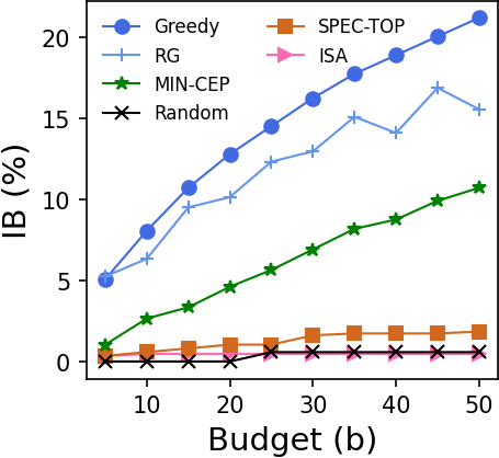
(a) NYC Cab

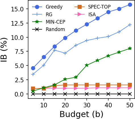
(b) NYC Cab

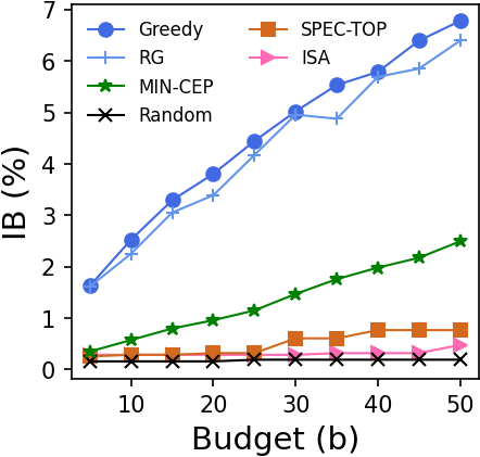
(c) NYC Cab

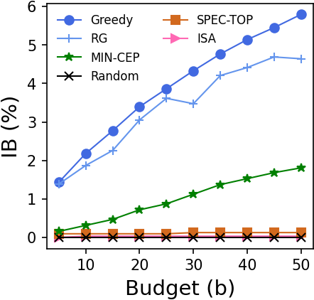
(d) NYC Cab

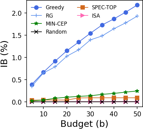
(e) NYC Cab

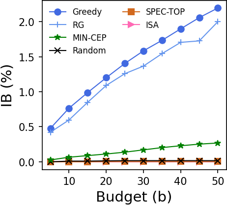
(f) NYC Cab

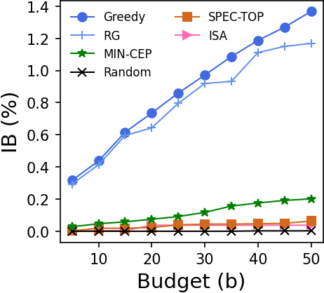
(g) NYC Cab

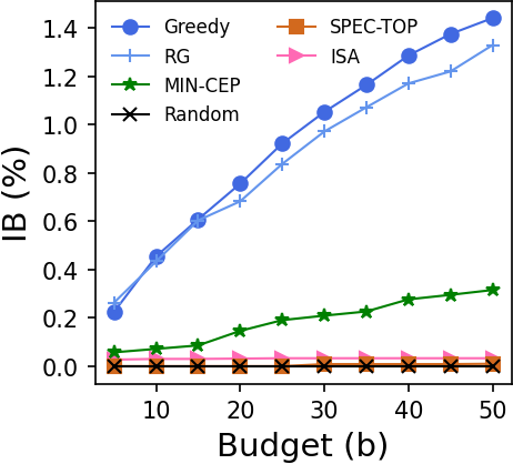
(h) WikiPolitics

Figure 2. Impact of budget on IB% (Eq. 5). Rg and Greedy are superior by up to $7$ times than the closest baseline (Min-Cep).

5.1. Experimental Setup

All algorithms have been implemented in Python $3.6.9$ on a Ubuntu $18.04$ PC with a $2.1$ GHz Intel^® Xeon^® Platinum $8160$ processor, $256$ GB RAM and a $7200$ RPM, $8.5$ TB disk. The codebase is available online.

5.1.1. Datasets

We use publicly available signed networks from http://konect.cc. Table 3 summarizes the dataset statistics. Each of these models polarized (signed) social interactions. BitcoinOTC, BitcoinAlpha, Epinions are trust/distrust networks on the two respective Bitcoin trading platforms and an online product rating site respectively. Chess represents the chess games’ results with edges being positive if white won and negative otherwise. Slashdot comprises the friend/foe relations on the news site Slashdot. The edges in WikiConflict represent the positive/negative conflicts on the Wikipedia. WikiPolitics contains interpreted interactions between editors of political articles on Wikipedia. WikiElections connects Wikipedia users who voted for/against each other. We ignore the direction of the edges in the directed graphs and remove any loops and multi-edges.

5.1.2. Baselines

Besides Greedy and Randomized Greedy (Rg), we consider the following baselines:

• Spec-Top: In §3.1, we design a spectral approach using an upperbound of the minimum eigen value of the Laplacian.

• Isa: Alg. 1 describes this baseline, which is based on perturbation theory. We only consider the peripheral edges as the candidates.

• Random: We randomly delete $b$ edges from the periphery of $S(H)$, where $H$ is the initial given subgraph.

• Min-Cep: Obs. 3 shows that an edge ($e$) deletion associated with a node $x$ is favorable if $|cep(H_{\{e\}},x)|=0$. Thus, we iteratively delete the peripheral edge minimizing $|cep(H_{\{e\}},x)|$.

5.1.3. Parameters:

The default input subgraph $H$ is the largest connected component (LCC) of the signed graph. We find the initial maximum balanced graph $S(H)$ using TIMBAL (Ordozgoiti et al., 2020). Table 3 lists the size of the LCC and its balance in each of the datasets. In addition, for some experiments, we also use $k$-core structures that are well-known for community discovery (Peng et al., 2014). The set of candidate edges $\mathbb{C}$ is set to all edges in $H$. The budget $b$ is varied in each experiment.

5.1.4. Performance Metric:

The quality of a solution (edge) set $B$ for a given subgraph $H$ is defined as the percentage of nodes that gets included in the balanced subgraph after the deletion of $B$.

(5) $$IB(B,H)(\%)=\frac{\Delta(H_{B})-\Delta(H)}{|H|-\Delta(H)}\times 100.$$

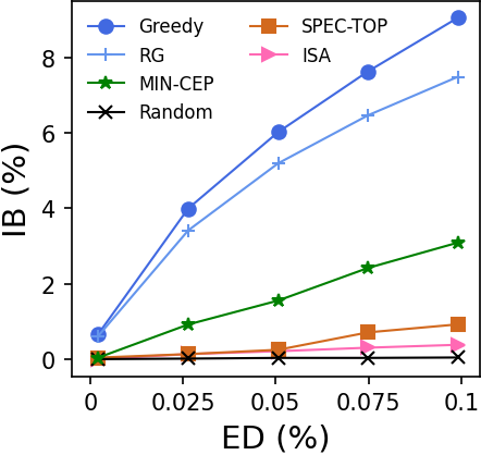
(a) NYC Cab

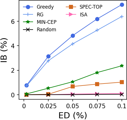
(b) NYC Cab

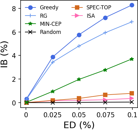
(c) NYC Cab

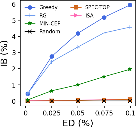
(d) NYC Cab

Figure 3. The quality of all methods with large budgets (ED implies the fraction of edge deletions) in four large datasets.

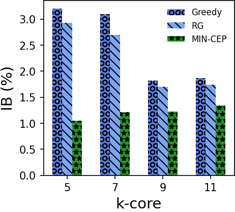
(a) NYC Cab

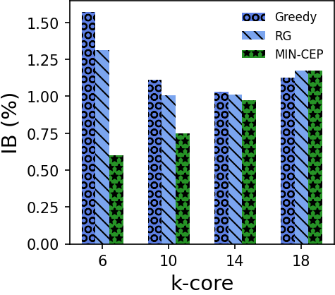
(b) NYC Cab

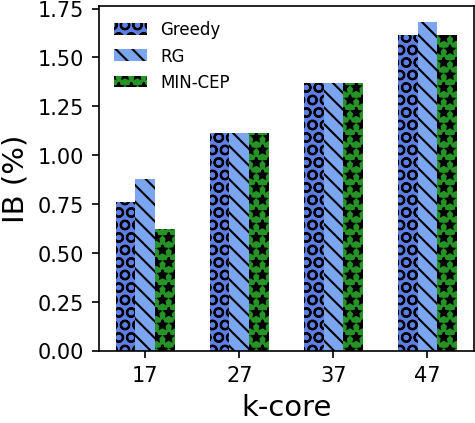
(c) NYC Cab

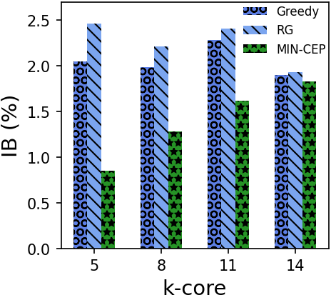
(d) NYC Cab

Figure 4. Increase in the balance when the input subgraph is a $k$-core. Results are shown against varying values of $k$ for $b=50$.

5.2. Efficacy and Efficiency

5.2.1. Small budget on all datasets:

Fig. 2 shows the percentage increase in balance (IB) for eight datasets achieved by each algorithm. Greedy and Rg outperform all the baselines by up to 12%. Besides having approximation guarantees (Thms. 3 and 4), Greedy and Rg directly optimize the objective function in an iterative fashion. In contrast, the baselines choose solution edges depending on other criterion. In particular, the spectral methods Isa and Spec-Top do not perform well since it chooses edges based on an upper-bound to minimize the minimum eigenvalue of the corresponding Laplacian. Though the balanced graph has minimum eigenvalue of the Laplacian as $0$, the rate at which the edge deletions move towards achieving it, might still be low. We also observe that Greedy, in general, performs better than Rg. It would be wrong, however, to draw the conclusion that Greedy is always better. In subsequent experiments where we choose $k$-cores as the input subgraphs, we will see that Rg performs better. We will revisit the topic of Greedy vs Rg while discussing that experiment.

5.2.2. Larger budget on large datasets:

To further demonstrate the efficacy of our methods we vary the budget as a function of $\mathbb{C}$. i.e., all edges in $H$. Fig. 3 shows the percentage increase in balance (IB) for the four largest datasets. Consistent with previous experiments, Rg and Greedy outperform all baselines (better by up to $6\%$ points). More interestingly, we observe that a substantial increase in balance is feasible ($9\%$ or up to $4000$ nodes) by deleting only $0.1\%$ of edges ($\approx 500$ edges). In other words, improvement in balance-dependent community functions, such as team performance or stability, may be significantly improved through minor adjustments to the network.

5.2.3. Scalability:

Table 4 shows the running times of all algorithms against budget in the three largest datasets. Although Rg and Greedy are slower than the other baselines, they finish within a few minutes even on a million edges’ network. Thus, scalability to large networks is not a concern. A more interesting behavior is witnessed in the correlation between efficacy and efficiency. More specifically, we observe that the better performance of an algorithm in IB%, the higher is its running time. When an algorithm performs better, it means in each iteration, the algorithm produces a larger cascading impact following an edge deletion. Higher cascading impact leads to a larger number of new peripheral edges coming into consideration. Consequently, the running time goes up.

	Epinions			WikiPolitics			WikiConflict
	10	30	50	10	30	50	10	30	50
Isa	2	6	11	2	7	12	4	12	19
Spec-Top	2	6	9	3	9	15	3	7	11
Min-Cep	4	5	6	4	6	7	10	12	14
Rg	6	7	9	7	9	10	13	16	18
Greedy	7	13	18	9	18	25	15	22	28

Table 4. Running times in minutes of the algorithms varying budget on largest available datasets.

5.3. Impact of Community Density

In this experiment, we systematically vary the density of the input community $H$ and analyze its impact on the performance. To control the density of $H$, we use $k$-core (Zhang et al., 2017) as the input subgraph. As $k$ increases, $H$ gets denser. Table 5 shows the maximum and minimum $k$-core sizes along with their balance for each dataset. We vary the value of $k$ depending on the $k$-core distribution of the graph. As high $k$-cores contain fewer nodes, the highest value of $k$ is chosen such that the size of the $k$-core is at least $10\%$ of the original graph size in terms of number of nodes.

Fig. 4 presents the results. In this section, we only consider the three best-performing algorithms of Greedy, Rg and Min-Cep. Greedy and Rg continue to be the best performers. Another interesting behavior we observe is that, the higher the $k$, and therefore density, the smaller is the gap between Greedy and Rg. In some cases, Rg performs better than Greedy. This behavior is a direct consequence of how Rg and Greedy operates. Greedy deterministically chooses the edge with the highest marginal gain. Consequently, when the gradient of the marginal gains in the sorted order is high, choosing the highest edge produces a good result. However, when the gradient is small and several edges provide similarly high marginal gains, Rg performs better.

5.4. Visualizations on Bitcoin Network

In the next experiment, we visually inspect the impact of edge deletions on increasing balance in the BitcoinOTC data. Fig. 5 presents the gradual increase in the size of the balanced component following $5$ and $10$ edge deletions. It shows that: (1) both positive and negative edges are chosen for deletion, and (2) there may be significant cascading impact of a single deletion (as visible in the appearance of several new green squares in Fig. 5(c)).

6. Conclusions

In this paper, we studied the problem of maximizing the balance in signed networks via edge deletion. While existing studies have focused primarily on finding the largest balanced subgraph, we adopted a network design approach to improve balance inside a subgraph. We proved that the problem is NP-hard, non-submodular, and non-monotonic. To overcome the resultant computational challenges, we designed an efficient heuristic based on the relation of Laplacian eigenvalues with the balance in corresponding signed graphs. Since these heuristics do not exhibit approximation guarantees, we leverage pseudo-submodularity of the objective function to design greedy algorithms with provable approximation guarantees. Through an extensive set of experiments, we showed that the proposed approximation algorithms outperform the baseline algorithms while being scalable to large graphs. An interesting future direction would be to explore alternative network design mechanisms such as node deletion and edge-sign flips to improve balance. From a theoretical perspective, we also aim to investigate the parameterized complexity of balance-related design problems.

Datasets	$|V(H_{k_{min}})|$	$|\Delta(H_{k_{min}})|$	$|V(H_{k_{max}})|$	$|\Delta(H_{k_{max}})|$
Epinions	26k	20k	13k	10k
Slashdot	23k	14k	8k	4k
WikiConflict	25k	17k	12k	9k
WikiPolitics	37k	30k	14k	11k

Table 5. Sizes of the $k$-core ($H_{k}$) corresponding to the minimum ($H_{k_{min}}$) and maximum ($H_{k_{max}}$) values of $k$ considered for each dataset in Fig. 4.

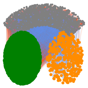
(a) NYC Cab

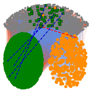
(b) NYC Cab

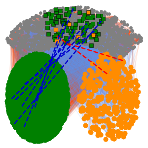
(c) NYC Cab

Figure 5. Visualization of the impact of edge deletions by Greedy. Green and orange denote the two partitions of the balanced subgraph $S(H)$; grey denotes the component outside $S(H)$. The solid red and blue edges are positive and negative edges, respectively, while the dashed edges in (b) and (c) are the ones being deleted. (b) and (c) also show the new components being added to the balanced portion through green and orange squares.

7. Appendix

7.1. Proof of Lemma 7

Proof.

Given a signed graph $G=(V,E,\sigma)$, a subgraph $H$, let $\lambda_{i}$, $\tilde{\lambda_{i}}$ be the eigenvalues of $L(H)$ and the perturbed matrix $\hat{L}(H)$ (after single edge $(i,j)$ deletion) respectively where $\lambda_{1}\leq\lambda_{2}\leq\cdots\leq\lambda_{m}$.

We have $\hat{L}(H)=L(H)+P$, and perturbation matrix $P=\bar{D}+S$, where $\bar{D}$ is a diagonal matrix with $\bar{D}_{ii}=\bar{D}_{jj}=-1$ and $0$ otherwise. $S_{ij}=S_{ji}=\sigma(i,j)$ for the perturbed edge $(i,j)\in E$ and otherwise $0$. Given $\bm{v}$ as the unit eigenvector corresponding to $\lambda_{1}$ we have,

$$\bm{v}^{T}\bar{D}\bm{v}=\sum_{k=i,j}\bar{D}_{kk}v^{2}_{k},\text{ and }\bm{v}^{T}S\bm{v}=\sum_{i,j}\sigma(i,j)v_{i}v_{j}$$

From the first-order matrix perturbation theory (see p. 183 (Stewart and Sun, 1990)),

$$\tilde{\lambda}_{1} =\lambda_{1}+\bm{v}^{T}P\bm{v}+O(||P||^{2}_{F})=\lambda_{1}+\bm{v}^{T}\bar{D}\bm{v}+\bm{v}^{T}S\bm{v}+O(||P||^{2}_{F})$$

$$=\lambda_{1}-\sum_{k=i,j}v^{2}_{k}+\sum_{i,j}\sigma(i,j)v_{i}v_{j}+O(1)$$

$$=\lambda_{1}-v_{i}(v_{i}-\sigma(i,j)v_{j})-v_{j}(v_{j}-\sigma(j,i)v_{i})+O(1)$$

$$=\lambda_{1}-\left(v_{i}-\sigma(i,j)v_{j}\right)^{2}+O(1)$$

Now, to show that $\tilde{\lambda_{1}}(H)$ is indeed the smallest eigenvalue of $\hat{L}(H)$, using matrix perturbation theory (p. 203 (Stewart and Sun, 1990)), we have

$$\tilde{\lambda_{1}} \leq\lambda_{1}+||P||_{2}\leq\lambda_{1}+||P||_{F}\leq\lambda_{1}+2$$

$$\tilde{\lambda_{i}} \geq\lambda_{i}-||P||_{2}\geq\lambda_{i}-||P||_{F}\geq\lambda_{i}-2,~{}(i\geq 2)$$

Since the spectral gap $\delta=\lambda_{2}-\lambda_{1}\geq 4$, we have $\tilde{\lambda_{i}}\geq\tilde{\lambda_{1}}$. So, we have $\tilde{\lambda_{1}}=\hat{\lambda}_{1}$ is the smallest eigenvalue of $\hat{L}(H)$. ∎

7.2. Details for proof for Theorem 2

Before proving Thm. 2, we derive a few results. Let $\hat{\mathbb{V}}$ be the node set that gets added in the maximum balanced subgraph $S(H)$ after deleting $B$ edges. We know that $\forall u\in\hat{\mathbb{V}}$ there exists $v\in S(H)$ such that $(u,v)\in B$. The inclusion of one node may lead to including more nodes in the balanced portion. Let $C_{u}$ be the size of component that gets added with $u\in\hat{\mathbb{V}}$ and $C^{*}=\max\{C_{u},\>u\in\hat{\mathbb{V}}\}$.

Observation 4.

(6) $$C^{*}+1\leq\frac{\Delta(H)}{2}\vspace{-0.05in}$$

Proof by Contradiction. If $|C_{u}|>\frac{\Delta(H)-2}{2}$, then the initial $S(H)$ would consist of the larger among $V_{1}$ and $V_{2}$ (which would be at least of size $\frac{\Delta(H)}{2}$) along with $\{u\}\cup C_{u}$.

Choice of $\alpha(B)$ and Peripheral Edges (PE): Let $\alpha(B)$ be the number of nodes $x$ satisfying: (1) $|cep(H_{\{e\}},x)|>0,\forall e\in B$ and (2) $|cep(H_{Y},x)|=0$ for some subset $Y\subseteq B,Y\neq\emptyset$. We use Obs. 3 to restrict the edge set $B$ to always belong to the periphery of the current balanced subgraph. An upperbound of $f(B)$ is as follows.

Lemma 9.

(7) $$f(B)\leq\sum_{i=1}^{b}{f(\{e_{i}\})}+(C^{*}+1)\alpha(B).$$

Proof.

This is proved using induction (Sec. 8.4). ∎

7.2.1. Final proof for Theorem 2

Proof.

Note that $f(Q\cup R)-f(Q)=\Delta(H_{Q\cup R})-\Delta(H_{Q})$. We can write this as $\Delta(H^{\prime}_{R})-\Delta(H^{\prime})$, where $H^{\prime}=H_{Q}$. That means marginal gain in balance of deleting the set $R$ over $Q$ is same as the marginal gain in balance of deleting the set $R$ from $H_{Q}$. We can thus use $f^{\prime}(R)=\Delta(H^{\prime}_{R})-\Delta(H^{\prime})$ in place of $f$. Thus, by Lem. 9:

(8) $$f^{\prime}(B)\leq\sum_{i=1}^{b}{f^{\prime}(\{e_{i}\})}+(C^{*}+1)\alpha(B)$$

where $C^{*}$ and $\alpha$ are defined accordingly to new initial subgraph $H^{\prime}=H_{Q}$. Next, we propose an upper bound of $\alpha(.)$ as follows:

(9) $$\alpha(B)\leq\frac{|B|-1}{2}$$

This is true since we need at least two edges for one node to be counted in $\alpha(B)$.

$$\begin{split}\text{Now we have, }\frac{\sum_{e\in R}{[f(Q\cup\{e\})-f(Q)]}}{f(Q\cup R)-f(Q)}=\frac{\sum_{e\in R}{f^{\prime}(\{e\})}}{f^{\prime}(R)}\\ \geq\frac{1}{1+\frac{\alpha(R)(C^{*}+1)}{\sum_{e\in R}{f^{\prime}(\{e\})}}}\left(\text{ Replace $f^{\prime}(R)$ using Eq. \ref{eq:f_dash}}\right)\\ \end{split}$$

$$\begin{split}\geq\frac{1}{1+\frac{\frac{|R|-1}{2}(C^{*}+1)}{\sum_{e\in R}{f^{\prime}(\{e\})}}}\left(\text{ Using the upper bound of $\alpha$ in Eq. \ref{eq:alpha_ub} }\right)\\ \geq\frac{1}{1+\frac{1}{4}\Delta(H_{Q})(|R|-1)}\left(\text{$\sum_{e\in R}{f^{\prime}(e)}\geq 1,C^{*}+1\leq\frac{\Delta(H_{Q})}{2}$ [Eq. \ref{eq:C_star}]}\right).\end{split}$$

∎

We also show a construction for the tight lower bound in Thm. 2 (Sec. 8.5).

7.3. Proof with bound $\frac{4\psi^{r}}{4\psi^{r}+\Delta^{RG}(b-1)}$

In proof of Thm. 2, we have $\sum_{e\in R}{f^{\prime}(e)}\geq 1$. However, $\sum_{e\in R}{f^{\prime}(e)}\geq\psi^{r}$, where $\psi^{r}$ is the summation of marginal gains of the elements in the optimal solution set (i.e., $R$) over the solution set produced by Rg (i.e., $Q$). Now replacing $\sum_{e\in R}{f^{\prime}(e)}$, as $\psi^{r}$ we get, $\gamma^{\prime}\geq\frac{4\psi^{r}}{4\psi^{r}+\Delta^{RG}(b-1)}$ according to Thm. 3.

7.4. Approximation by Greedy

Lemma 10 ((Das and Kempe, 2018)).

Given $f$ is a non-negative and monotone set function, budget $b$, and $\sum_{e\in R}{[f(S^{G}\cup\{e\})-f(S^{G}))]}\geq\gamma\cdot[f(S^{G}\cup R)-f(R)]$ where $S^{G}$ is the final set selected by the Greedy Algorithm, then the algorithm has the following approximation guarantee of $(1-e^{-\gamma_{S^{G},b}})$ where $\gamma_{S^{G},b}=min\{\gamma\}$ for any $R,S^{G}\cap R=\Phi$.

We apply this result in our problem setting:

Theorem 4.

For the MBED problem, Greedy algorithm obtains an approximation of $1-e^{-\gamma^{\prime}}$, and $\gamma^{\prime}\geq\frac{4}{4+\Delta^{*}(b-1)}$ where $b$ and $\Delta^{*}$ denote the budget and the balance after deleting the optimal set of edges respectively.

Proof.

Let the optimal set of $b$ edges be $B^{*}$ and let $S^{G}$ denote the final edge set by the Greedy algorithm. Also, let $\Delta^{*}$ denote the balance after deleting the optimal set of edges, then by its definition we have $\Delta(H_{S^{G}})\leq\Delta^{*}$. From Theorem 2, $\gamma^{\prime}=\gamma_{S^{G},|B^{*}|}\geq\frac{4}{4+\Delta(H_{S^{G}})(|B^{*}|-1)}\geq\frac{4}{4+\Delta^{*}(b-1)}$. So, substituting $\gamma_{S^{G},b}$ in Lem. 10 as $\gamma_{S^{G},|B^{*}|}$ (or $\gamma^{\prime}$), we get the desired approximation of $\frac{4}{4+\Delta^{*}(b-1)}$. ∎

The other lowers bounds for $\gamma^{\prime}$ (where the approximation produced by Greedy is $1-e^{-\gamma^{\prime}}$) as $\frac{4}{4+\Delta^{G}(b-1)}$ and $\frac{4\psi^{g}}{4\psi^{g}+\Delta^{G}(b-1)}$ can be derived in similar ways as in the case of Rg.

8. Additional proofs

8.1. NP-hardness

Proof.

Let $SK(U,S,P,W,q)$ be an instance of the Set Union Knapsack Problem (Goldschmidt et al., 1994), where $U=\{u_{1},\ldots u_{n}\}$ is a set of items, $S=\{S_{1},\ldots S_{m}\}$ is a set of subsets ($S_{i}\subseteq U$), $P:S\to\mathbb{R}_{+}$ is a subset profit function, $w:U\to\mathbb{R}_{+}$ is an item weight function, and $q\in\mathbb{R}_{+}$ is the budget. For a subset $\mathcal{A}\subseteq S$, the weighted union of set $\mathcal{A}$ is $W(\mathcal{A})=\sum_{e\in\cup_{t\in\mathcal{A}}S_{t}}w_{e}$ and $P(\mathcal{A})=\sum_{t\in\mathcal{A}}p_{t}$. The problem is to find a subset $\mathcal{A}^{*}\subseteq S$ such that $W(\mathcal{A}^{*})\leq q$ and $P(\mathcal{A}^{*})$ is maximized. SK is NP-hard to approximate within a constant factor (Arulselvan, 2014). We reduce a version of $SK$ with equal profits and weights (also NP-hard) to the Mbed problem. We define a corresponding Mbed problem instance via constructing a graph $\Gamma$ as follows.

For each $S_{i}\in S$ and $u_{j}\in U$ we create nodes $x_{i}$ and $y_{j}$ respectively. We also add a node $v$ with a large connected component $L$ of size $l$ only with positive edges attached to it. The node $v$ has negative edges with every node $x_{i}$, $\forall i\in[m]$ and every node $y_{j}$, $\forall j\in[n]$. Additionally, if $u_{j}\in S_{i}$, a negative edge $(x_{i},y_{j})$ will be added to the edge set $E$.

In Mbed, the number of edges to be removed is the budget, $b=q$. The candidate set, $\mathbb{C}=\{(v,y_{j})|\forall j\in[n]\}$. Note that initial largest connected balanced component is $\{v\cup L\}\cup\{y_{j}\forall j\in[n]\}$ if $l>m+1$ (assuming $n>m$). Our claim is that, for any solution $\mathcal{A}$ of an instance of $SK$ there is a corresponding solution set of edges, $B$ (where $|B|=b$) in the graph $\Gamma$ of the Mbed version, such that $f(B)=P(\mathcal{A})+n+l+1$ if $B=\{(v,y)|y\in\mathcal{A}\}$ are removed.

In the new balanced graph, we aim to build two partitions ($W_{1}$ and $W_{2}$) as follows. One partition $W_{1}$ consists of $\{v\cup L\}$ initially. Our goal is to delete edges from $\mathbb{C}$ and add the nodes $y_{j}$’s in $W_{1}$. If $(v,y_{j^{\prime}})$ for any $j^{\prime}$ does not get deleted then it would be in $W_{2}$. If there is any node $x_{i}$ that is connected with only nodes in $\mathcal{A}$ beside being connected with $v$, then removing all the edges in $B$ would put the node $x_{i}$ in $W_{2}$. Thus removing edges in $\mathcal{A}$ would put $P(\mathcal{A})$ nodes in $W_{2}$. Thus, $f(B)=P(\mathcal{A})+n+l+1$.

∎

8.2. Proportionally Submodular

Lemma 8.1.

The objective function $f$ is not proportionally
submodular (Santiago and Yoshida, 2020). In other words, there exists $S,T\in E$ for some graph $H$ such that $|T|f(S)+|S|f(T)<|S\cap T|f(S\cup T)+|S\cup T|f(S\cap T)$.

Proof.

Consider a balanced subgraph of $H$, $S(H)$ has a partition $V_{1}$ and $V_{2}$. A node $v$ is outside $S(H)$ and it is connected to $V_{1}$ with positive edges $e_{1}$ and $e_{2}$, $V_{2}$ with another positive edge $e_{3}$. Thus the node $v$ cannot be the part of $S(H)$. Consider an edge $e_{4}$ inside $V_{1}$ which can be removed without making the graph disconnected. Let us assume $S=\{e_{1},e_{4}\},T=\{e_{2},e_{4}\}$. Then, $f(\{e_{1},e_{4}\})=0$ and $f(\{e_{2},e_{4}\})=0$, since even after removing any of these edges it is not possible to add the node $v$ to $S(H)$. Note that $f(S\cap T)=f(\{e_{4}\})=0$. However, $f(S\cup T)=f(\{e_{1},e_{2},e_{4}\})=1$ since the node $v$ can be added. Substituting these values, we get $|T|f(S)+|S|f(T)<|S\cap T|f(S\cup T)+|S\cup T|f(S\cap T)$. ∎

8.3. Proof of Lemma 6

We denote $g_{X}(Y)$ as the marginal gain of the set of edges $Y$ over the set $X$, i.e., $g_{X}(Y)=g(X\cup Y)-g(X)$. To prove modularity, we need to show $g_{X}(Y)=\sum_{e\in Y}{g_{X}(e)}$, i.e. the marginal gain of the set of $Y$ over $X$ is the summation of the marginal gains of each individual in $Y$ over $X$ for any $X,Y$.

Proof.

We can write $g_{X}(Y)$ as follows.

$$g_{X}(Y) =-\sum_{(i,j)\in X\cup Y}{{(\bm{v}_{i}-\sigma(i,j)\bm{v}_{j})}^{2}}+\sum_{(i,j)\in X}{{(\bm{v}_{i}-\sigma(i,j)\bm{v}_{j})}^{2}}$$

$$=-\sum_{(i,j)\in Y}{{(\bm{v}_{i}-\sigma(i,j)\bm{v}_{j})}^{2}}=\sum_{e\in Y}{g_{X}(e)}$$

∎

8.4. Proof of Lemma 9

Proof.

We prove this by induction on the number of edges, $b$. Let us denote $B_{k}\subseteq B$ as $\{e_{1},\cdots,e_{k}\}$. We construct $B$ by only considering peripheral edges $e_{k+1}$ such that, for all $k\leq b$: $(e_{k+1},e^{\prime})\in cep(H_{B_{k}},x)$, for some node $x$ and edge $e^{\prime}$.

Base case $(b=1)$: $f(\{e_{1}\})\leq f(\{e_{1}\})$. Also, $\alpha(\{e_{1}\})=0$.

Inductive hypothesis (IH): Suppose the equation holds for $b=k$, i.e., $f(B_{k})\leq\sum_{i=1}^{k}{f(\{e_{i}\})}+(C^{*}+1)\alpha(B_{k})$.

Inductive step $(b=k+1)$: We present different cases for $e_{k+1}$. Note that we have $(e_{k+1},e^{\prime})\in cep(H_{B_{k}},x)$ for some $x,e^{\prime}$.

Case 1: $(e_{k+1},e^{\prime})\in cep(H,x)$ and $\left|cep\left(H_{e_{k+1}},x\right)\right|=0$, i.e., after deleting $e_{k+1}$, $x$ moves into the balanced subgraph. Then, we must also have $\left|cep\left(H_{B_{k+1}},x\right)\right|=0$. Hence, $f(B_{k}\cup\{e_{k+1}\})-f(B_{k})=f(\{e_{k+1}\})$ and the inequality holds.

Case 2: Either (1) $(e_{k+1},e^{\prime})\in cep(H,x)$ and $\left|cep\left(H_{e_{k+1}},x\right)\right|>0$ or (2) $(e_{k+1},e^{\prime})\notin cep(H,x)$.

Thus, by Observation 2, we have $f(\{e_{k+1}\})=0$.

Case 2a: Suppose $\left|cep\left(H_{B_{k+1}},x\right)\right|=0$. Then by definition of $\alpha,C^{*}$, we have $\alpha(B_{k+1})=\alpha(B_{k})+1$, and $f(\{B_{k}\cup e_{k+1}\})-f(B_{k})\leq C^{*}+1$.

Substituting this, we get $f(B_{k+1})\leq(C^{*}+1)+\sum_{i=1}^{k}{f(\{e_{i}\})}+(C^{*}+1)\alpha(B_{k})=\sum_{i=1}^{k+1}{f(\{e_{i}\})}+(C^{*}+1)\alpha(B_{k+1})$.

Case 2b: In other cases, $f(B_{k}\cup\{e_{k+1}\})-f(B_{k})=f(\{e_{k+1}\})=0$.

This exhausts our cases and the claim is true $\forall b,b>0$. ∎

8.5. Construction for the tight lower bound in Thm. 2

One can construct a graph $H$ and the sets $Q,R$ where equality holds. In particular, let $R$ be of an arbitrary size $b$. Consider $H_{Q}$ to have the MBS partition as $V_{1},V_{2}$ each of size $\frac{\Delta(H_{Q})}{2}$. Nodes of type 1 (Obs. 2) are attached to these each with the sole connected component of size $\frac{\Delta(H_{Q})-2}{2}$. Let these nodes have 3 such connections (thus, removing two will help - any two such that our ”connected assumption” holds are in the set $R$). We have another node of type 1 such that only two such connections are connected and one of these is in $R$ and the connected component $C$ to it is of size $0$. This completes the set $R$. Thus, $\sum_{e\in R}{[f(Q\cup\{e\})-f(Q)}=1$ and $f(Q\cup R)-f(Q)=1+\left(\frac{\Delta(H_{Q})-2}{2}+1\right)\frac{b-1}{2}$.

References

- (1)
- Akiyama et al. (1981) Jin Akiyama, David Avis, Vasek Chvátal, and Hiroshi Era. 1981. Balancing signed graphs. Discrete Applied Mathematics 3, 4 (1981), 227–233.
- Arulselvan (2014) Ashwin Arulselvan. 2014. A note on the set union knapsack problem. Discrete Applied Mathematics 169 (2014), 214–218.
- Askarisichani et al. (2019) O. Askarisichani, J. Ng Lane, F. Bullo, N. E. Friedkin, A. K. Singh, and B. Uzzi. 2019. Structural Balance Emerges and Explains Performance in Risky Decision-Making. 10, 2648 (2019). https://doi.org/10.1038/s41467-019-10548-8
- Belardo (2014) Francesco Belardo. 2014. Balancedness and the least eigenvalue of Laplacian of signed graphs. Linear Algebra Appl. 446 (2014), 133–147.
- Chaoji et al. (2012) Vineet Chaoji, Sayan Ranu, Rajeev Rastogi, and Rushi Bhatt. 2012. Recommendations to boost content spread in social networks. In WWW. 529–538.
- Coakley and Rokhlin (2013) Ed S Coakley and Vladimir Rokhlin. 2013. A fast divide-and-conquer algorithm for computing the spectra of real symmetric tridiagonal matrices. Applied and Computational Harmonic Analysis 34, 3 (2013), 379–414.
- Crescenzi et al. (2015) Pierluigi Crescenzi, Gianlorenzo D’Angelo, Lorenzo Severini, and Yllka Velaj. 2015. Greedily Improving Our Own Centrality in A Network. In SEA. Springer International Publishing, 43–55.
- Das and Kempe (2018) A. Das and D. Kempe. 2018. Approximate submodularity and its applications: subset selection, sparse approximation and dictionary selection. The Journal of Machine Learning Research 19, 1 (2018), 74–107.
- DasGupta et al. (2007) Bhaskar DasGupta, German Andres Enciso, Eduardo Sontag, and Yi Zhang. 2007. Algorithmic and complexity results for decompositions of biological networks into monotone subsystems. Biosystems 90, 1 (2007), 161–178.
- Dey and Medya (2020) Palash Dey and Sourav Medya. 2020. Manipulating Node Similarity Measures in Network. In AAMAS.
- Dilkina et al. (2011) Bistra Dilkina, Katherine J. Lai, and Carla P. Gomes. 2011. Upgrading shortest paths in networks. In Integration of AI and OR Techniques in Constraint Programming for Combinatorial Optimization Problems. Springer, 76–91.
- Figueiredo and Frota (2014) Rosa Figueiredo and Yuri Frota. 2014. The maximum balanced subgraph of a signed graph: Applications and solution approaches. European Journal of Operational Research 236, 2 (2014), 473–487.
- Garimella and Weber (2017) Venkata Rama Kiran Garimella and Ingmar Weber. 2017. A long-term analysis of polarization on Twitter. In Eleventh International AAAI Conference on Web and Social Media.
- Goldschmidt et al. (1994) Olivier Goldschmidt, David Nehme, and Gang Yu. 1994. Note: On the set-union knapsack problem. Naval Research Logistics (NRL) (1994).
- Harary et al. (1953) Frank Harary et al. 1953. On the notion of balance of a signed graph. The Michigan Mathematical Journal 2, 2 (1953), 143–146.
- Hou et al. (2003) Yaoping Hou, Jiongsheng Li, and Yongliang Pan. 2003. On the Laplacian eigenvalues of signed graphs. Linear and Multilinear Algebra 51, 1 (2003), 21–30.
- Hüffner et al. (2007) Falk Hüffner, Nadja Betzler, and Rolf Niedermeier. 2007. Optimal edge deletions for signed graph balancing. In International Workshop on Experimental and Efficient Algorithms. Springer, 297–310.
- Ishakian et al. (2012) Vatche Ishakian, Dóra Erdos, Evimaria Terzi, and Azer Bestavros. 2012. A Framework for the Evaluation and Management of Network Centrality. In Proc. SIAM International Conference on Data Mining. 427–438.
- Kempe et al. (2003) David Kempe, Jon Kleinberg, and Éva Tardos. 2003. Maximizing the spread of influence through a social network. In KDD.
- Kimura et al. (2008) Masahiro Kimura, Kazumi Saito, and Hiroshi Motoda. 2008. Minimizing the Spread of Contamination by Blocking Links in a Network.. In AAAI.
- Knyazev (2001) Andrew V Knyazev. 2001. Toward the optimal preconditioned eigensolver: Locally optimal block preconditioned conjugate gradient method. SIAM journal on scientific computing 23, 2 (2001), 517–541.
- Li and Li (2009) Hong-hai Li and Jiong-sheng Li. 2009. Note on the normalized Laplacian eigenvalues of signed graphs. Australasian J. Combinatorics 44 (2009), 153–162.
- Lin and Mouratidis (2015) Yimin Lin and Kyriakos Mouratidis. 2015. Best upgrade plans for single and multiple source-destination pairs. GeoInformatica 19, 2 (2015), 365–404.
- Medya et al. (2020) Sourav Medya, Tiyani Ma, Arlei Silva, and Ambuj Singh. 2020. A Game Theoretic Approach For Core Resilience. In Proceedings of the Twenty-Ninth International Joint Conference on Artificial Intelligence, IJCAI-20.
- Medya et al. (2020) S. Medya, A. Silva, and A. Singh. 2020. Approximate Algorithms for Data-driven Influence Limitation. IEEE Transactions on Knowledge and Data Engineering (2020).
- Medya et al. (2018a) Sourav Medya, Arlei Silva, Ambuj Singh, Prithwish Basu, and Ananthram Swami. 2018a. Group centrality maximization via network design. In Proc. 24th SIAM International Conference on Data Mining. SIAM, 126–134.
- Medya et al. (2018b) Sourav Medya, Jithin Vachery, Sayan Ranu, and Ambuj Singh. 2018b. Noticeable network delay minimization via node upgrades. Proceedings of the VLDB Endowment 11, 9 (2018), 988–1001.
- Meyerson and Tagiku (2009) Adam Meyerson and Brian Tagiku. 2009. Minimizing average shortest path distances via shortcut edge addition. In Approximation, Randomization, and Combinatorial Optimization. Algorithms and Techniques (APPROX-RANDOM). Springer, 272–285.
- Mitra et al. (2015) Shubhadip Mitra, Sayan Ranu, Vinay Kolar, Aditya Telang, Arnab Bhattacharya, Ravi Kokku, and Sriram Raghavan. 2015. Trajectory aware macro-cell planning for mobile users. In 2015 IEEE Conference on Computer Communications (INFOCOM). IEEE, 792–800.
- Nemhauser and Wolsey (1978) George L Nemhauser and Laurence A Wolsey. 1978. Best algorithms for approximating the maximum of a submodular set function. Mathematics of operations research 3, 3 (1978), 177–188.
- Ordozgoiti et al. (2020) Bruno Ordozgoiti, Antonis Matakos, and Aristides Gionis. 2020. Finding large balanced subgraphs in signed networks. In Proceedings of The Web Conference 2020. 1378–1388.
- Orecchia et al. (2012) Lorenzo Orecchia, Sushant Sachdeva, and Nisheeth K Vishnoi. 2012. Approximating the exponential, the Lanczos method and an O (m)-time spectral algorithm for balanced separator. In Proceedings of the forty-fourth annual ACM symposium on Theory of computing. 1141–1160.
- Paulheim (2017) Heiko Paulheim. 2017. Knowledge graph refinement: A survey of approaches and evaluation methods. Semantic web 8, 3 (2017), 489–508.
- Peng et al. (2014) Chengbin Peng, Tamara G Kolda, and Ali Pinar. 2014. Accelerating community detection by using k-core subgraphs. arXiv preprint arXiv:1403.2226 (2014).
- Poljak and Turzík (1986) Svatopluk Poljak and Daniel Turzík. 1986. A polynomial time heuristic for certain subgraph optimization problems with guaranteed worst case bound. Discrete Mathematics 58, 1 (1986), 99–104.
- Santiago and Yoshida (2020) Richard Santiago and Yuichi Yoshida. 2020. Weakly Submodular Function Maximization Using Local Submodularity Ratio. arXiv preprint arXiv:2004.14650 (2020).
- Stewart and Sun (1990) G.W. Stewart and J-g Sun. 1990. Matrix Perturbation Theory. Academic Press, Inc.
- Zhang et al. (2017) Fan Zhang, Ying Zhang, Lu Qin, Wenjie Zhang, and Xuemin Lin. 2017. Finding Critical Users for Social Network Engagement: The Collapsed k-Core Problem. In Thirty-First AAAI Conference on Artificial Intelligence. 245–251.
- Zhou et al. (2019) Zhongxin Zhou, Fan Zhang, Xuemin Lin, Wenjie Zhang, and Chen Chen. 2019. K-Core Maximization: An Edge Addition Approach.. In IJCAI. 4867–4873.