Multi-Dimensional Randomized Response

Abstract

In our data world, a host of not necessarily trusted controllers gather data on individual subjects. To preserve her privacy and, more generally, her informational self-determination, the individual has to be empowered by giving her agency on her own data. Maximum agency is afforded by local anonymization, that allows each individual to anonymize her own data before handing them to the data controller. Randomized response (RR) is a local anonymization approach able to yield multi-dimensional full sets of anonymized microdata that are valid for exploratory analysis and machine learning. This is so because an unbiased estimate of the distribution of the true data of individuals can be obtained from their pooled randomized data. Furthermore, RR offers rigorous privacy guarantees. The main weakness of RR is the curse of dimensionality when applied to several attributes: as the number of attributes grows, the accuracy of the estimated true data distribution quickly degrades. We propose several complementary approaches to mitigate the dimensionality problem. First, we present two basic protocols, separate RR on each attribute and joint RR for all attributes, and discuss their limitations. Then we introduce an algorithm to form clusters of attributes so that attributes in different clusters can be viewed as independent and joint RR can be performed within each cluster. After that, we introduce an adjustment algorithm for the randomized data set that repairs some of the accuracy loss due to assuming independence between attributes when using RR separately on each attribute or due to assuming independence between clusters in cluster-wise RR. We also present empirical work to illustrate the proposed methods.

1 Introduction

Twenty years ago, National Statistical Institutes and a few others were the only data controllers explicitly gathering data on citizens, and their legal status often made them trusted. In contrast, in the current big data scenario, there is a host of controllers gathering information, and it is no longer reasonable to take it for granted that the individual subject trusts all of them to keep her data confidential and/or to anonymize them properly in case of release [23].

Thus, to preserve her privacy and, more generally, her informational self-determination, the individual has to be empowered by giving her agency on her own data. Local anonymization is a paradigm in which each individual anonymizes her data before handing them to the data controller, thereby giving maximum agency to the individual. Several masking methods coming from statistical disclosure control (SDC [16]) can be applied locally, including generalization/recoding and noise addition. On the other hand, there are methods specifically designed for local anonymization that, in addition to helping subjects hide their responses, allow the data controller to get an accurate estimation of the distribution of responses for groups of subjects (for example, randomized response [32, 15] and FRAPP [1]). Also, a number of methods have been proposed to obtain differentially private (DP) preselected statistics via local anonymization, like RAPPOR [12] and local DP [6, 5].

While most of the local anonymization approaches were designed to obtain statistics on the set of individuals who contribute their locally anonymized input, randomized response (RR) has the attractive feature of being able to output multi-dimensional full sets of anonymized microdata (individual records) that are valid for exploratory analysis. Indeed, an unbiased estimate of the distribution of the original microdata (corresponding to the true attribute values of individuals) can be obtained from the empirical distribution of the released randomized microdata. Most exploratory analyses and statistical calculations can be performed based on this estimated distribution, including what [10] call multi-party computation with statistical input confidentiality. It is even possible to re-create a synthetic estimate of the original data set by repeating each combination of attribute values as many times as dictated by its frequency in the estimated joint distribution.

Furthermore, the privacy guarantees afforded by RR are easily expressible in terms of rigorous privacy models such as differential privacy [31, 30] or information-theoretic secrecy [9].

Unfortunately, the picture is not as rosy as suggested by the two previous paragraphs. Like so many methods, randomized response suffers from the curse of dimensionality:

• Applying RR simultaneously to a set of attributes amounts to applying it to the Cartesian product of those attributes, which has a number of possible categories that grows exponentially with the number of attributes. Unless the number of individuals providing input is much greater than the number of categories, the accuracy and hence the utility of the estimated distribution of the original data will be poor.

• RR can certainly be applied separately to each single attribute. Nevertheless, by doing so the ability to estimate the joint distribution of the original data based on the randomized data is lost; only the marginal distributions of attributes can be estimated. This also entails a loss of accuracy and hence a loss of utility of the estimated distributions.

Dimensionality issues are common to all data anonymization techniques. However, effectively dealing with them is tougher in the local anonymization paradigm because the global picture of the data is missing. Research in this topic is ample. In particular, in differential privacy and local differential privacy, many strategies have been proposed to cope with a high number of attributes, such as dealing with $k$-way marginals [35, 22, 34], taking advantage of sparsity [33, 6] or taking advantage of the dependence between attributes [29, 17].

Contribution and plan of this paper

In this paper, we propose several complementary approaches to mitigate the curse of dimensionality in randomized response. The paper’s contributions are as follows:

• We first present two basic protocols for RR and discuss their limitations: one performs separate RR for each attribute and the other joint RR for all attributes.

• We then describe an intermediate approach based on identifying clusters of attributes such that attributes in different clusters can be viewed as (nearly) independent. In this way, joint RR can be performed for the attributes in each cluster. Since our clustering algorithm requires as input the dependences between attributes, we present several methods for assessing these dependences in an RR scenario in which the true data of each individual must stay confidential to that individual.

• After that, we introduce an adjustment algorithm of the randomized data set that “repairs” some of the accuracy loss incurred by assuming independence between attributes when using RR separately on each attribute or assuming independence between clusters when using RR cluster-wise.

Section 2 gives background on RR, its privacy guarantees and its estimation error. Section 3 introduces the two basic RR protocols: separate RR for each attribute and joint RR for all attributes. Section 4 presents the approach based on attribute clustering and the methods for privacy-preserving evaluation of attribute dependences. Section 5 details the adjustment to reduce the accuracy loss caused by the independence assumptions. Experimental work is reported in Section 6. Section 7 reviews related work. Finally, conclusions and future research directions are gathered in Section 8.

2 Background

2.1 Randomized response

Randomized response [32, 15] is a mechanism that respondents to a survey can use to protect their privacy when asked about the value of sensitive attribute (e.g. did you take drugs last month?). In many respects RR was a forerunner when proposed in the 1960s: it was not only an anonymization method avant la lettre (before anonymization and statistical disclosure control were introduced by Dalenius [8] a decade later), but it ushered in the even more modern notion of local anonymization. Closely related to RR are the more recent PRAM [19] and FRAPP [1] methods. PRAM, which stands for post-randomization method, differs from RR on who performs the randomization [28]: whereas in RR it is the individual before delivering her response, in PRAM it is the data controller after collecting all responses (hence the name post-randomization). FRAPP extends the original RR method along the lines proposed in [4].

Beyond historical merit, a strong point of RR is that the data collector can still estimate from the randomized responses the proportion of each of the possible true answers of the respondents.

Let us denote by $X$ the attribute containing the answer to the sensitive question. If $X$ can take $r$ possible values, then the randomized response $Y$ reported by the respondent instead of $X$ follows an $r\times r$ matrix of probabilities

$${\bf P}=\left(\begin{array}[]{ccc}p_{11}&\cdots&p_{1r}\\ \vdots&\vdots&\vdots\\ p_{r1}&\cdots&p_{rr}\end{array}\right),$$ (1)

where $p_{uv}=\Pr(Y=v|X=u)$, for $u,v\in\{1,\ldots,r\}$ denotes the probability that the randomized response is $v$ when the respondent’s true attribute value is $u$.

Let $\pi_{1},\ldots,\pi_{r}$ be the proportions of respondents whose true values fall in each of the $r$ categories of $X$ and let $\lambda_{v}=\sum_{u=1}^{r}p_{uv}\pi_{u}$ for $v=1,\ldots,r$, be the probability of the reported value $Y$ being $v$. If we define ${\bf\lambda}=(\lambda_{1},\ldots,\lambda_{r})^{T}$ and ${\bf\pi}=(\pi_{1},\ldots,\pi_{r})^{T}$, it holds that ${\bf\lambda}={\bf P}^{T}{\bf\pi}$. Furthermore, if $\hat{\bf\lambda}$ is the vector of sample proportions corresponding to ${\bf\lambda}$ and ${\bf P}$ is nonsingular, in Chapter 3.3 of [4] it is proven that an unbiased estimator ${\bf\pi}$ can be computed as

$$\hat{\bf\pi}=({\bf P}^{T})^{-1}\hat{\bf\lambda}$$ (2)

and an unbiased estimator of the dispersion matrix is also provided. In particular, the larger the off-diagonal probability mass in ${\bf P}$, the more dispersion (and the more respondent protection).

The estimation obtained from Equation (2) may not be a proper probability distribution: it may have values below 0 and above 1. This happens when the empirical distribution of the randomized data is not consistent with the randomization matrix. For instance, if all the values in the first column of ${\bf P}$ are greater than 0.5, then we should expect the frequency of the first category to be greater than 0.5. If it is not, then Equation (2) will necessarily return some negative values. In [2] an iterative Bayesian update is proposed that converges to a proper probability distribution. In Section 6.4, we describe a simpler solution to ensure a proper distribution.

2.2 Privacy guarantees

The confidentiality guarantee given by RR results from each individual potentially altering her response by randomly drawing from a previously fixed distribution. Thus, given the individual’s randomized response, we are uncertain about what her true response would have been.

In spite of the previous intrinsic guarantee of randomized response and given the popularity of differential privacy [11], we will also quantify the privacy afforded by randomized response in terms of differential privacy. However, we would like to remark that attaining a given level of differential privacy is not the goal of this work. Among the algorithms we propose, some enforce differential privacy while others only qualify as differentially private if certain assumptions are made about the information that is publicly available. While we do not claim that such algorithms are differentially private, we would like to note that making assumptions about externally available information is usual (e.g. see invariants in [14]).

A randomized query function $\kappa$ gives $\epsilon$-differential privacy if, for all data sets $D_{1}$, $D_{2}$ such that one can be obtained from the other by modifying a single record, and all $S\subset Range(\kappa)$, it holds

$$\Pr(\kappa(D_{1})\in S)\leq\exp(\epsilon)\times\Pr(\kappa(D_{2})\in S).$$ (3)

In plain words, the presence or absence of any single record is not noticeable (up to $\exp(\epsilon)$) when seeing the outcome of the query. Hence, this outcome can be disclosed without impairing the privacy of any of the potential respondents whose records might be in the data set. A usual mechanism to satisfy Inequality (3) is to add noise to the true outcome of the query, in order to obtain an outcome of $\kappa$ that is a noise-added version of the true outcome. The smaller $\epsilon$, the more noise is needed to make queries on $D_{1}$ and $D_{2}$ indistinguishable up to $\exp(\epsilon)$.

In [31, 30], a connection between randomized response and differential privacy is established: randomized response is $\epsilon$-differentially private if

$$e^{\epsilon}\geq\max_{v=1,\ldots,r}\frac{\max_{u=1,\ldots,r}p_{uv}}{\min_{u=1,\ldots,r}p_{uv}}.$$ (4)

The rationale is that the values in each column $v$ ($v\in\{1,\ldots,r\}$) of matrix ${\bf P}$ correspond to the probabilities of the reported value being $Y=v$, given that the true value is $X=u$ for $u\in\{1,\ldots,r\}$. Differential privacy requires that the maximum ratio between the probabilities in a column be bounded by $e^{\epsilon}$, so that the influence of the true value $X$ on the reported value $Y$ is limited. Thus, the reported value can be released with limited disclosure of the true value.

2.3 Frequency estimation error

We want to minimize the error in the estimation of $\hat{\bf\pi}$. Following Equation (2), the error in $\hat{\bf\pi}$ comes from two sources: (i) the error in the estimation of $\hat{\bf\lambda}$, and (ii) the propagation of that error when computing the product $({\bf P}^{T})^{-1}\hat{\bf\lambda}$.

Following [1], the propagation error is lower-bounded by $P_{max}/P_{min}$, where $P_{max}$ and $P_{min}$ are the maximum and minimum eigenvalues of ${\bf P}^{T}$. Indeed, [1] show that to minimize the propagation of the error the randomization matrix must have the form

$${\bf P}=\left(\begin{array}[]{cccc}p_{u}&p_{d}&\cdots&p_{d}\\ p_{d}&p_{u}&\ddots&\vdots\\ \vdots&\ddots&\ddots&p_{d}\\ p_{d}&\cdots&p_{d}&p_{u}\end{array}\right),$$

with $p_{u}\geq p_{d}$. Provided we use a randomization matrix that minimizes the propagation of the error, the error in $\hat{\bf\pi}$ is a function of the error in $\hat{\bf\lambda}$. In the rest of this section, we bound the error in the estimation of $\hat{\bf\lambda}$.

We can view the sample of $Y$ as a draw from a multinomial distribution with $n$ trials (the data set size) and probabilities $\lambda$. Thus, it is natural to derive the estimate $\hat{\lambda}$ from the observed frequencies of $Y$. Let us deal with the accuracy of $\hat{\lambda}$, which in [27] is measured using confidence intervals as follows.

Definition 1.

The absolute error of $\hat{\lambda}$ as an estimation of $\lambda$ is $e_{abs}$ with confidence $\alpha$ if

$$\Pr[\bigcap_{u=1,\ldots,r}(\hat{\lambda}_{u}-e_{abs}\leq\lambda_{u}\leq\hat{\lambda}_{u}+e_{abs})]\geq 1-\alpha.$$

The absolute error can be determined, based on the frequencies and the data set size, as

$$e_{abs}=\max_{u=1,\ldots,r}\sqrt{B\lambda_{u}(1-\lambda_{u})/n},$$ (5)

where $B$ is the $\alpha/r$ upper percentile of the $\chi^{2}$ distribution with 1 degree of freedom.

The absolute error grows with $\sqrt{B}$, which in turn grows with the number of categories $r$ as shown in Figure 1. While the impact $r$ on the absolute error via $\sqrt{B}$ seems limited, the actual effect of increasing $r$ on Expression (5) can be greater. The reason is that increasing the number of categories decreases the absolute frequency of each category, which makes the relative error of $\hat{\lambda}$ more noticeable.

Figure 1: Evolution of the factor $\sqrt{B}$ ($y$-axis) of the absolute error of $\hat{\lambda}$ in terms of the number of categories $r$ ($x$-axis) when $\alpha=0.05$

Definition 2.

The relative error of $\hat{\lambda}$ as an estimation of $\lambda$ is $e_{rel}$ with confidence $\alpha$ if

$$\Pr[\bigcap_{u=1,\ldots,r}((1-e_{rel})\hat{\lambda}_{u}\leq\lambda_{u}\leq(1+e_{rel})\hat{\lambda}_{u}]\geq 1-\alpha.$$

Analogously to Expression (5), we can determine the relative error based on the frequencies and the data set size:

$$e_{rel}=\max_{u=1,\ldots,r}\sqrt{B\frac{1-\lambda_{u}}{\lambda_{u}}\frac{1}{n}},$$ (6)

where $B$ is the $\alpha/r$ upper percentile of the $\chi^{2}$ distribution with 1 degree of freedom.

3 Basic RR protocols: RR-Independent and RR-Joint

Assume $n$ parties $i=1,\ldots,n$ each holding one record ${\bf x}_{i}=(x^{1}_{i},$ $\ldots,$ $x^{m}_{i})$ that contains the values for $m$ attributes. A data controller wants to perform exploratory analysis and/or machine learning tasks on the pooled data of the $n$ parties. However, no party wants to disclose her true record even if she is ready to disclose a masked version of it.

In the above situation RR is a good option, as motivated in the previous sections. In this section we describe two basic RR methods to estimate the pooled true data of the parties, and we also highlight the limitations of such methods.

3.1 RR-Independent

This is the most naive solution. Each party $i$ separately deals with each attribute value $x_{i}^{j}$ for $j=1,\ldots,m$ via RR. If the $j$-th attribute $A^{j}$ can take $r^{j}$ different values, then an $r^{j}\times r^{j}$ probability matrix ${\bf P}^{j}$ (see Expression (1)) can be used for each party to report a randomized value $y_{i}^{j}$ for $A^{j}$ instead of her true value $x_{i}^{j}$. See Protocol 1.

Protocol 1 RR-Independent

1. Randomization Protocol

2. Let $x_{i}^{j}$ be the value of party $i$ for attribute $j$.

3. Let ${\bf P}^{j}$ be the randomization matrix for attribute $j$.

4. Each party $i=1,\ldots,n$ applies RR with matrix ${\bf P}^{j}$ to $x_{i}^{j}$, for $j=1,\ldots,m$, and publishes the result.

5. Attribute Distribution Estimation

6. Let $\hat{\lambda}^{j}$ be the experimental distribution of the randomized attribute $A^{j}$.

7. The distribution of $A^{j}$ is estimated as $\hat{\pi}^{j}=(({\bf P}^{j})^{T})^{-1}\hat{\lambda^{j}}$.

8. Joint Distribution Estimation

9. Let ${\bf S}\subset A^{1}\times\ldots\times A^{m}$ be a subset of the data domain.

10. The frequency of ${\bf S}$ is estimated as $\sum_{(x^{1},\ldots,x^{m})\in{\bf S}}\hat{\pi}^{1}(x^{1})\times\ldots\times\hat{\pi}^{m}(x^{m})$.

As mentioned in Section 2.1, this would allow all parties to approximate the marginal empirical distribution ${\bf\pi}^{j}=(\pi^{j}_{1},\ldots,\pi^{j}_{r^{j}})$ of each attribute $A^{j}$ as

$$\hat{\bf\pi}^{j}=(({\bf P}^{j})^{T})^{-1}\hat{\bf\lambda}^{j},$$

where $\hat{\bf\lambda}^{j}$ is the empirical distribution of attribute $A^{j}$ in the data set ${\bf Y}$ containing the randomized responses.

The problem is that estimating the marginal empirical distributions of attributes does not yield in general an estimate of the joint empirical distribution of the data set ${\bf X}$ formed by the true responses. Only if the attributes in ${\bf X}$ are (nearly) independent can their joint distribution be estimated from the marginal attribute frequencies. In this case, the frequency of a set ${\bf S}\subset A^{1}\times\ldots\times A^{m}$ can be estimated as $\sum_{(x^{1},\ldots,x^{m})\in{\bf S}}\hat{\pi}^{1}(x^{1})\times\ldots\times\hat{\pi}^{m}(x^{m})$. Clearly, the more dependent the attributes, the less accurate is the previous estimate.

With respect to the computational cost, the fact that each attribute is dealt with separately is positive because the randomization matrices remain small. The computational complexity for each of the individuals that participate in the protocol is as follows:

• Estimating the distribution of the true values of attribute $A^{j}$ as per Expression (2) amounts to computing the inverse of an $|A^{j}|$-dimensional matrix followed by an $|A^{j}|$-dimensional matrix-vector product. The actual cost is dominated by the matrix inversion. If using Strassen’s algorithm (the best-performing practical algorithm,  [26]), inversion takes $\mathcal{O}(|A^{j}|^{2.807})$. In the particular case of the randomization matrices described in Section 2.3, their regularity makes it possible to easily compute their inverses with a cost $\mathcal{O}(|A^{j}|^{2})$.

• The cost of estimating the joint frequency of one combination of attribute values is $\mathcal{O}(m)$.

3.2 RR-Joint

To estimate the frequency of an arbitrary set ${\bf S}\subset A^{1}\times\ldots\times A^{m}$ without requiring attribute independence, we need to directly estimate the joint distribution. To do this via RR, each party must report her randomized response for the value of $A^{1}\times\ldots\times A^{m}$. After this, the frequency of a set ${\bf S}\subset A^{1}\times\ldots\times A^{m}$ can be estimated as $\sum_{{\bf x}\in{\bf S}}({\bf P}^{T})^{-1}\hat{\bf\lambda}({\bf x})$, where $\hat{\bf\lambda}(\bf x)$ is the empirical distribution of x in ${\bf Y}$. See Protocol 2.

Two observations are in order. First, thanks to RR, all parties preserve the confidentiality of their true inputs during Protocol 2. Second, once the estimate of the empirical joint distribution of ${\bf X}$ is published, any parties can perform statistical computations on it; they can even create a synthetic data set by repeating each combination of $A^{1}\times A^{2}\times\ldots\times A^{m}$ as many times as dictated by its frequency in the joint distribution.

Protocol 2 RR-Joint

1. Randomization Protocol

2. Let ${\bf x}_{i}$ be the record of party $i$.

3. Let ${\bf P}$ be the randomization matrix of $A^{1}\times\ldots\times A^{m}$.

4. Each party $i=1,\ldots,n$ runs RR with matrix ${\bf P}$ on ${\bf x}_{i}$ and publishes the result.

5. Joint Distribution Estimation

6. Let ${\bf S}\subset A^{1}\times\ldots\times A^{m}$ be a subset of the data domain.

7. The frequency of ${\bf S}$ is estimated as $\sum_{{\bf x}\in{\bf S}}({\bf P}^{T})^{-1}\hat{\lambda}({\bf x})$.

Unfortunately, direct estimation of the joint distribution is not without limitations. As the number of attributes grows linearly, the number of categories of the Cartesian product grows exponentially. This causes the computational cost to increase and the accuracy of the frequency estimates to decrease in ways that are not acceptable.

The high computational cost comes from having a vector of frequencies of exponential size $\Pi_{j=1,\ldots,m}|A^{j}|$ and a (huge) randomization matrix with $\Pi_{j=1,\ldots,m}|A^{j}|$ rows and the same number of columns. According to Expression (2), to estimate $\hat{\pi}$ we need to multiply the inverse of the transpose of the randomization matrix times $\hat{\lambda}$. Even if we assume that the (computationally costly) inverse matrix is available so that we only need to perform the matrix multiplication, the cost remains exponential in the number of attributes.

Regarding the accuracy of the frequency estimates, direct estimation of the joint distribution only works well if the number of parties $n$ is much larger than the number of possible values of the above Cartesian product, that is, when

$$n\gg|A^{1}|\times|A^{2}|\times\ldots\times|A^{m}|.$$ (7)

The necessity of Bound (7) becomes obvious when we analyze the error as per Expression (6) for $n=|A^{1}|\times|A^{2}|\times\ldots\times|A^{m}|=r$. Even if frequencies $\lambda_{u}$ were evenly distributed and equal to $1/r$ —which would minimize their relative estimation error—, Expression (6) would yield approximately $\sqrt{B}$. By looking at Figure 1, we observe that $\sqrt{B}$ is too big (above $200\%$) to be acceptable as a relative error.

3.3 Accuracy analysis

Let us compare the relative error achieved by Protocols RR-Independent and RR-Joint. As above, we will perform the analysis in the best case, that is, when frequencies are evenly distributed.

Thus, for R-Independent we take $\lambda^{j}_{u}=1/|A^{j}|$ for all $j=1,\ldots,m$ and all $u=1,\ldots,|A^{j}|$. According to Expression (6), the relative error of attribute frequencies in RR-Independent is

$$e_{rel}=\max_{j=1,\ldots,m}\sqrt{B^{j}\frac{|A^{j}|-1}{n}},$$

where $B^{j}$ is the $(\alpha/|A^{j}|)$ upper percentile of a $\chi^{2}$ distribution with one degree of freedom.

Similarly, the relative error of the estimated frequencies in RR-Joint is

$$e_{rel}=\sqrt{B\frac{\Pi_{j=1,\ldots,m}|A^{j}|-1}{n}},$$

where $B$ is the $(\alpha/\Pi_{j=1,\ldots,m}|A^{j}|)$ upper percentile of a $\chi^{2}$ distribution with one degree of freedom.

Notice that the relative error grows as the square root of the number of categories, which is exponential in the number of attributes. Thus, RR-Joint is likely to have poor accuracy estimates already for a small number of attributes. As described in Section 3.2, this can only be mitigated by a large data set size $n$, which becomes unrealistic already for a moderate number of attributes.

4 RR-Clusters

Neither Protocol RR-Independent nor Protocol RR-Joint are satisfactory, the former due to the independence requirement and the latter due to the combinatorial explosion of the number of categories. In this section, we propose RR-Clusters, a protocol that strives to use as little as possible the independence assumption, while keeping a reasonable computational cost and estimation accuracy.

The RR-Clusters protocol splits attributes into clusters according to their mutual dependence and performs RR-Joint independently on each of the attribute clusters.

Running RR-Joint separately on each attribute cluster implies neglecting the possible dependences between attributes in different clusters. Thus, we need to determine clusters in such a way that no significant dependence exists between any two attributes in different clusters.

Additionally, to keep the computational cost and the estimation error within reasonable bounds, we want the cardinality of the Cartesian product of attributes within each cluster to be small compared with the number of records of the data set. Thus, the clustering algorithm should try to place in the same cluster only those attributes that have a strong mutual dependence.

More specifically, we want a set of clusters $C_{1},\ldots,C_{l}$, for some $l$, such that:

• $\bigcup_{k=1,\ldots,l}C_{k}=\{A^{1},\ldots,A^{m}\}$ and $C_{i}\cap C_{j}=\emptyset$ for $i\neq j$;

• It holds that $n\gg\max_{k=1,\ldots,l}\Pi_{j\in C_{k}}|A^{j}|$;

• The dependence between attributes in different clusters is as low as possible.

Since attributes are to be clustered based on their dependences, we start by describing the clustering algorithm assuming that those dependences are available. Computing the dependences between attributes would be easy if one could resort to a trusted party holding the entire data set. Lacking a trusted party, we need methods to assess attribute dependence without requiring parties to disclose their data. We describe such methods in Sections 4.1, 4.2 and 4.3; they differ in their accuracy and in the disclosure risk for the parties’ true attribute values.

The clustering algorithm is formalized in Algorithm 1. It starts with single-attribute clusters. It then loops through the list of cluster pairs in descending order of dependence, and merges two clusters if the number of combinations of attribute values in the merged cluster remains below a given threshold. Additionally, to avoid clustering attributes that are not really dependent, the algorithm uses a threshold on the dependence measure below which clusters are not merged. The dependence between two clusters of attributes is defined as the maximum dependence between pairs of attributes such that one attribute is in one cluster and the other attribute is in the other cluster.

Algorithm 1 Clustering of attributes based on their dependence

1. Let $T_{v}$ be the maximum number of combinations of attribute values allowed in a cluster

2. Let $T_{d}$ be the minimum dependence required between two clusters for them to be merged

3. Let $Clusters=\{\{A^{1}\},\ldots,\{A^{m}\}\}$

4. Let $DependenceList$ be the list of dependences between cluster pairs

5. Sort $DependenceList$ in descending order

6. Let $dep$ be the first element of $DependenceList$

7. While $dep\geq T_{d}$ do

8. Let $(C_{1},C_{2})$ be the cluster pair whose dependence is $dep$

9. If $\Pi_{A\in C_{1}\cup C_{2}}|A|\leq T_{v}$ then

10. Remove $C_{1}$ and $C_{2}$ from $Clusters$

11. Add $C_{1}\cup C_{2}$ to $Clusters$

12. Recompute $DependenceList$ for $Clusters$

13. Sort $DependenceList$ in descending order

14. Let $dep$ be the first element of $DependenceList$

15. Else

16. Let $dep$ be the next element of $DependenceList$

17. End if

18. End while

The specific measure of dependence to be used must take into account the type of the attributes. We will use the following dependence metrics adopted in [10]. If $A^{i}$ and $A^{j}$ are ordinal, we can take as a measure of dependence

$$|r_{ij}|,$$ (8)

where $r_{ij}$ is Pearson’s correlation coefficient between $A^{i}$ and $A^{j}$. Expression (8) can also be used for continuous numerical attributes, but to be accommodated by RR these need to be discretized into ordinal attributes (for example by rounding or by replacing values with intervals).

If one of $A^{i}$ and $A^{j}$ is nominal (without an order relationship between its possible values) and the other is nominal or ordinal, we can take as a measure of independence

$$V_{ij},$$ (9)

where $V_{ij}$ is Cramér’s V statistic [7], that gives a value between 0 and 1, with 0 meaning complete independence between $A^{i}$ and $A^{j}$ and 1 meaning complete dependence. Cramér’s $V_{ij}$ is computed as

$$V_{ij}=\sqrt{\frac{\chi^{2}_{ij}/n}{\min(r^{i}-1,r^{j}-1)}},$$

where $r^{i}$ is the number of categories of $A^{i}$, $r^{j}$ is the number of categories of $A^{j}$, $n$ is the total number of parties/records and $\chi^{2}_{ij}$ is the chi-squared independence statistic defined as

$$\chi^{2}_{ij}=\sum_{a=1}^{r^{i}}\sum_{b=1}^{r^{j}}\frac{(o^{ij}_{ab}-e^{ij}_{ab})^{2}}{f^{j}_{ab}},$$

with $o^{ij}_{ab}$ the observed frequency of the combination $(A^{i}=a,A^{j}=b)$ and $e^{ij}_{ab}$ the expected frequency of that combination under the independence assumption for $A^{i}$ and $A^{j}$. This expected frequency is computed as

$$e^{ij}_{ab}=\frac{n^{i}_{a}n^{j}_{b}}{n},$$

where $n^{i}_{a}$ and $n^{j}_{b}$ are, respectively, the number of parties who have reported $A^{i}=a$ and $A^{j}=b$.

Finally, if one of $A^{i},A^{j}$ is nominal and the other is numerical, the latter must be discretized. After that, the contingency table between $A^{i}$ and $A^{j}$ can be constructed, and the measure of dependence given by Expression (9) can be computed.

Note that Expressions (8) and (9) are bounded in $[0,1]$, and hence the outputs of both expressions are comparable when trying to cluster the attributes.

With respect to the computational cost, the fact that the number of combinations of attribute values within each cluster is relatively small (because each cluster contains only a subset of attributes) leads to a set of randomization matrices of relatively small size; this is positive to keep the computational cost reasonable. The computational cost for each of the individuals that participate in the protocol is as follows:

• Estimating the joint distribution of the true values of attributes in cluster $C_{k}$ as per Expression (2) amounts to computing the inverse of a $\prod_{A\in C_{k}}|A|$-dimensional matrix followed by a $\prod_{A\in C_{k}}|A|$-dimensional matrix-vector product. As far as the order is concerned we can overlook the less costly matrix-vector product. As to the cost of computing the inverse matrix, with Strassen’s algorithm it is $\mathcal{O}(\prod_{A\in C_{k}}|A|^{2.807})$.

• The cost of estimating the joint frequency of one combination of attribute values is $\mathcal{O}(l)$, where $l$ is the number of clusters.

Since ${\bf X}$ is formed by the true responses of the parties and these do not disclose them, no single party can compute the dependences between the attributes in ${\bf X}$. In the following subsections, we describe several methods to compute such dependences based on partial and/or inaccurate information submitted by the individual parties. Each method has a different level of accuracy as well as a different impact on privacy. The overall privacy risk is the aggregation of the risk that results from the computation of the dependences between attributes and the risk that results from applying RR to the resulting clusters of attributes. In differential privacy terms, the sequential composition property applies [18]: if the computation of the dependences between attributes is $\epsilon_{1}$-differentially private and the RR data release is $\epsilon_{2}$-differentially private, overall one has $\epsilon_{1}+\epsilon_{2}$-differential privacy.

In Subsection 4.1, we describe an efficient method for computing the dependences between the attributes in ${\bf X}$ when the dependence measure is the covariance. Subsections 4.2 and 4.3 deal with arbitrary dependence measures and differ in the adversary model. Taking advantage of a common distinction between confidential and quasi-identifying attributes, Subsection 4.2 computes the dependence measure over each pairwise distribution of attributes. Subsection 4.3 avoids such a distinction and leverages randomized response to compute the dependences between attributes.

4.1 Randomized response on each attribute

In this section, we approximate the dependences between pairs of attributes based on a data set ${\bf Y}$ obtained by independently randomizing each attribute in ${\bf X}$ (see Section 3.1). Dependences between attributes in ${\bf Y}$ are likely to be attenuated versions of those in ${\bf X}$, but as long as the former dependences preserve the ranking of the latter, attribute clustering based on the former should be fine. In other words, if in ${\bf X}$ the dependence between $A^{1}$ and $A^{2}$ is stronger than the dependence between $A^{3}$ and $A^{4}$, our requirement is that the same relation hold in ${\bf Y}$.

To analyze the effect of RR on the dependence between attributes, we view each attribute of ${\bf X}$ as a random variable whose distribution is the empirical distribution of the attribute values. Note that this view is not entirely accurate, because it is unlikely that the same set of values is obtained if the attribute’s random variable is sampled. However, this is a useful approximation that significantly simplifies the analysis.

Proposition 1 examines the effect on the covariance between attributes when RR is independently run on each attribute. This proposition is later used in Corollary 1 to show that when RR is appropriately run, the relative strength of the covariances between pairs of attributes is not altered.

Proposition 1.

Let $X^{a}$ and $X^{b}$ be two finite random variables that are independently randomized into $Y^{a}$ and $Y^{b}$, respectively, as follows:

• With probability $p_{a}$ (resp. $p_{b}$), $Y^{a}:=X^{a}$ (resp. $Y^{b}:=X^{b}$).

• With probability $1-p_{a}$ (resp. $1-p_{b}$), $Y^{a}:=U^{a}$ (resp. $Y^{b}:=X^{b}$), where $U^{a}$ (resp. $U^{b}$) is a random variable that is uniformly distributed on the support of $X^{a}$ (resp. $X^{b}$).

Then the covariance of $Y^{a}$ and $Y^{b}$ is $Cov(Y^{a},Y^{b})=p_{a}\times p_{b}\times Cov(X^{a},X^{b})$.

Proof.

The covariance $Cov(Y^{a},Y^{b})$ can be expressed as

$$Cov(Y^{a},Y^{b})=E(Y^{a}Y^{b})-E(Y^{a})E(Y^{b}).$$ (10)

Let us start by computing $E(Y^{a})E(Y^{b})$. The expected values of $Y^{a}$ and $Y^{b}$ are $E(Y^{a})=p_{a}E(X^{a})+(1-p_{a})E(U^{a})$ and $E(Y^{b})=p_{b}E(X^{b})+(1-p_{b})E(U^{b})$. Their product is

$$E(Y^{a})E(Y^{b}) =p_{a}p_{b}E(X^{a})E(X^{b})$$

$$+p_{a}(1-p_{b})E(X^{a})E(U^{b})$$

$$+(1-p_{a})p_{b}E(U^{a})E(X^{b})$$

$$+(1-p_{a})(1-p_{b})E(U^{a})E(U^{b}).$$ (11)

Let us now compute $E(Y^{a}Y^{b})$. The random variable $Y^{a}Y^{b}$ can be expressed as:

$$Y^{a}Y^{b}=\begin{cases}X^{a}X^{b}&\text{with probability }p_{a}p_{b};\\ X^{a}U^{b}&\text{with probability }p_{a}(1-p_{b});\\ U^{a}X^{b}&\text{with probability }(1-p_{a})p_{b};\\ U^{a}U^{b}&\text{otherwise.}\end{cases}$$

Hence, $E(Y^{a}Y^{b})=p_{a}p_{b}E(X^{a}X^{b})+p_{a}(1-p_{b})E(X^{a}U^{b})+(1-p_{a})p_{b}E(U^{a}X^{b})+(1-p_{a})(1-p_{b})E(U^{a}U^{b})$. Since $U^{a}$ and $U^{b}$ are independent from each other and also are independent from $X^{a}$ and $X^{b}$, we can write the expected values as products:

$$E(Y^{a}Y^{b}) =p_{a}p_{b}E(X^{a}X^{b})+p_{a}(1-p_{b})E(X^{a})E(U^{b})$$

$$+(1-p_{a})p_{b}E(U^{a})E(X^{b})$$

$$+(1-p_{a})(1-p_{b})E(U^{a})E(U^{b}).$$ (12)

By plugging Expressions (11) and (12) into Expression (10) and simplifying, we can express the covariance as:

$$Cov(Y^{a},Y^{b}) =p_{a}p_{b}(E(X^{a}X^{b})-E(X^{a})E(X^{b}))$$

$$=p_{a}p_{b}Cov(X^{a},X^{b}).$$

∎

Corollary 1.

Let ${\bf X}$ be a data set with attributes $X^{1},\ldots,X^{m}$, that are randomized into $Y^{1},\ldots,Y^{m}$ as follows:

$$Y^{j}=\begin{cases}X^{j}&\text{with probability }p,\\ U^{j}&\text{otherwise,}\end{cases}$$

where $U^{j}$ is uniformly distributed over the support of $X^{j}$ and $p\in(0,1]$. Then the randomization does not alter the relative strength of the covariance between attributes, that is, if $Cov(X^{j},X^{k})>Cov(X^{l},X^{m})$ then $Cov(Y^{j},Y^{k})>Cov(Y^{l},Y^{m})$.

Proof.

The proof immediately follows from Proposition 1:

$$Cov(Y^{j},Y^{k}) =p^{2}Cov(X^{j},X^{k})>p^{2}Cov(X^{l},X^{m})$$

$$=Cov(Y^{l},Y^{m}).$$

∎

According to Proposition 1, RR attenuates the covariance between attributes, but Corollary 1 shows that it preserves the relative strength of the covariances between pairs of attributes. Since when clustering attributes with Algorithm 1 we are interested in the relative strength of the dependence between attributes, it makes sense to run Algorithm 1 using dependences between randomized attributes. Thus, attribute clusters can be obtained as follows:

1. Every party publishes the value of each of her attributes using RR with the randomization of Corollary 1.

2. Dependences are computed on the randomized attributes.

3. Algorithm 1 computes attribute clusters based on the dependences between randomized attributes.

As to the communication cost of this method, at least one individual must gather the entire randomized data set in order to compute attribute dependences and thereby the attribute clustering, which is then shared with the rest of individuals. Since the size of the randomized data set is $O(nm)$, the communication cost for the individual(s) computing the clustering is $O(nm)$. For the rest of individuals, the communication cost is only $O(m)$: they have to send their randomized record, then receive the attribute clustering and finally return their randomized record according to the received clustering. Regarding the computational cost, the computations are fairly simple for most individuals: they only need to randomize their records, which takes cost $O(m)$. For the individual(s) computing the dependences and the clustering of the $m$ attributes there is an additional cost that depends on the dependence measure and the clustering algorithm used.

In the above proposition and corollary, we have focused on covariance to measure dependence. Intuition tells us that the effect of randomization on other dependence measures, such as the ones mentioned in Section 4 for use with Algorithm 1, can be expected to be similar: attenuation of dependence but preservation of its relative strength. However, this need not always be the case —see Section 4.2 for a method that is agnostic of the dependence measure.

Once attribute clusters have been determined, parties can use RR-Joint within each cluster, which yields the final randomized data set.

Due to the fact that RR yields differential privacy (see Section 2.2), this method to compute the dependence between attributes yields differential privacy.

4.2 Exact bivariate distribution via secure sum

The method described in the previous section does not generalize to an arbitrary measure of dependence between attributes. In this section, we propose an alternative method that exploits the following two facts:

• We can remove identifier attributes from ${\bf X}$ without affecting its statistical utility;

• Bivariate distributions are enough to compute the dependence between pairs of attributes.

Essentially, the alternative procedure consists of each party releasing her true values for each pair of attributes, which yields bivariate distributions wherefrom attribute dependences are obtained. Note that, since parties release unmasked data, differential privacy does not apply. In spite of that, the risk of disclosure is low. Since ${\bf X}$ does not include identifiers, we are in one of the following situations:

• If none of the attributes of a given pair is confidential, then there is no risk of disclosure.

• If there is one confidential attribute (or two) in the pair, then intruders cannot re-identify the party to whom the record corresponds because there is (at most) one quasi-identifier attribute in the pair. Recall that a single quasi-identifier is not enough to re-identify a record (otherwise it would be an identifier).

The fact that a pair of attribute values is not re-identifying is of little help if the sender of the pair can be traced. Thus, we need the following:

• Anonymous communication. The communication channel should be anonymous. Otherwise, the identity of the party to whom a pair corresponds can be established by an intruder.

• Unlinkability of communications originated by a party. If an intruder can link several pairs of values originated by a party, he can acquire the values of several quasi-identifiers for that party, which may lead to her re-identification. Further, if confidential attributes are also among the acquired attributes, confidential information on the re-identified party has been disclosed.

The above properties can be attained by using a secure sum protocol. To illustrate how this can work to obtain the empirical distribution of two categorical attributes, we give a simple secure sum protocol that instantiates the general framework of [3]. Let $(a,a^{\prime})$ be a possible combination of values of attributes $A$ and $A^{\prime}$. To compute the absolute frequency of $(a,a^{\prime})$, $n$ parties proceed as follows:

1. Each party $i$ chooses a set of $n$ random numbers $r_{ij}$ such that $\sum_{j=1,\ldots,n}r_{ij}\pmod{n+1}=0$, that is, so that the sum of the chosen numbers is a multiple of $n+1$;

2. Each party $i$ sends $r_{ij}$ to party $j$, for each $j$;

3. Each party $j$ collects $r_{1j},\ldots,r_{nj}$, computes $\sum_{i=1,\ldots,n}r_{ij}$, and broadcasts:

   • $r_{j}=\sum_{i=1,\ldots,n}r_{ij}+1$ if attributes $A$ and $A^{\prime}$ take the values $a$ and $a^{\prime}$, respectively, for party $j$;

   • $r_{j}=\sum_{i=1,\ldots,n}r_{ij}$, otherwise;

4. Each party $i$ collects $r_{j}$ for $j=1,\ldots,n$ and computes the absolute frequency of $(a,a^{\prime})$ as $\sum_{j=1,\ldots,n}r_{j}\pmod{n+1}$.

Computing the frequency of every combination of values for each pair of attributes increases the communication cost with respect to the method of Subsection 4.1. Taking into account that the cost of the secure-sum protocol is proportional to the number of individuals $n$ and that it must be run for each possible value of each pair of attributes, the communication cost is $O(\sum_{1\leq i<j\leq m}(|A^{i}||A^{j}|)\times n)$. The computations needed to run the method in this subsection are fairly simple. For this reason, the overall cost is dominated by the communication cost.

4.3 Randomized response on each pair of attributes

The procedure described in Section 4.2 makes sure that only bivariate distributions are made available. Since a distribution does not report information on any specific party, its publication should in principle be safe. However, small frequencies are problematic as they may enable linking two or more pairs of values and this may lead to re-identification and disclosure. For example, if upon seeing the bivariate distribution of attribute $A^{1}$ and some other attribute $A^{2}$, an intruder learns there is a single party with $A^{1}=x$, then he can link all pairs $(A^{1}=x,A^{j})$ for $j\neq 2$ that have nonzero frequency and thereby rebuild the party’s entire record, which may lead to the party’s re-identification.

To prevent the above from happening, we can use RR on each pair of attributes, which renders the computation differentially private (see Section 2.2). The procedure is as follows:

1. Let $A^{1},\ldots,A^{m}$ be the attributes of data set ${\bf X}$;

2. Let ${\bf P}^{ij}$ be a randomization matrix for the pair of attributes $(A^{i},A^{j})$, for $1\leq i<j\leq m$;

3. For every pair $(A^{i},A^{j})$ of attributes:

   1. Each party uses ${\bf P}^{ij}$ to mask her value for the pair via RR;

   2. The $n$ parties engage in the secure sum protocol described in Section 4.2 to compute the distribution of the masked attribute pair;

   3. Each party uses Equation (2) to estimate the empirical distribution of the unmasked pair of attributes $(A^{i},A^{j})$ in ${\bf X}$.

Once the above procedure is complete, the dependence between any two attributes $A^{i}$ and $A^{j}$ can be assessed by all parties based on the estimated empirical distribution of $(A^{i},A^{j})$.

Notice that, in spite of using RR, the above procedure still resorts to the secure sum procedure: the purpose is to make each masked pair unlinkable to the party that originated it and also to make masked pairs corresponding to the same party unlinkable between them. Indeed, in the above procedure RR is computed $m-1$ times on each attribute (once for each other attribute in ${\bf X}$); if an intruder was able to link a party’s $m-1$ masked responses, the risk of disclosing the party’s true responses and identity would increase significantly.

If the randomization matrix is chosen adequately, this method to compute the dependence between attributes can achieve differential privacy, as recalled in Section 2.2. Strictly speaking, since each attribute is randomized and released $m-1$ times in the secure sum, sequential composition tells that the overall level of differential privacy is the sum of the levels of each release. However, the secure sum makes releases unlinkable, so an intruder cannot take advantage of the multiple releases to increase his knowledge about the value of an attribute. In this situation, we can waive sequential composition and take the overall level of differential privacy to be same as if each attribute were released only once: the unlinkability property closely matches the requirements of parallel composition.

The cost of the method in this subsection is easily computed by noticing that it is simply the method described in Subsection 4.2 with an additional randomization step. As the cost of the randomization step is not significant with respect to the cost of the secure sum, the cost of the method here equals that of Subsection 4.2: $O(\sum_{1\leq i<j\leq m}(|A^{i}||A^{j}|)\times n)$.

5 RR-Adjustment

To estimate the joint distribution in RR-Independent, we needed to assume that attributes were independent. We then proposed RR-Clusters to partially circumvent that need. We write “partially” because RR-Clusters still needs to assume that attributes in different clusters are independent. The purpose of the method described in this section, RR-Adjustment, is to “repair” some of the loss in estimation accuracy caused by these independence assumptions. The idea is to leverage the information about the relation between attributes that remains in the randomized data set in order to obtain more accurate estimates of the joint distribution.

Our description of RR-Adjustment will be given in terms of attributes. However, the same description is valid if we substitute clusters of attributes for attributes. Indeed, a cluster of attributes can also be viewed as a special attribute obtained as the Cartesian product of the attributes in the cluster. So where we write “attribute”, “marginal distribution” and “RR-Independent” in the rest of this section we could write “cluster of attributes”, “attribute cluster marginal distribution” and “RR-Clusters”, respectively.

RR-Adjustment is based on the fact that, although attenuated, the relation between attributes in ${\bf X}$ is likely to survive in ${\bf Y}$. The greater the probability that randomization preserves the true values (i.e. the greater the probability mass in the diagonal of the randomization matrix), the better the relation between attributes is preserved in ${\bf Y}$. For instance, when the RR matrix is the identity, ${\bf Y}$ contains the same information as ${\bf X}$. In contrast, when randomization replaces each true value by a draw from a uniform distribution, no information remains in ${\bf Y}$.

RR-Adjustment is formalized in Algorithm 2. The algorithm generates the estimate of the joint distribution of ${\bf X}$ by assigning weights (probabilities) to the records in ${\bf Y}$ in such a way that marginal distributions coincide with the estimates obtained from RR-Independent. An iterative approach is used in this task. Initially, each point of ${\bf Y}$ is assigned weight $1/n$. Then the algorithm loops through each attribute $A^{j}$ and adjusts the current weights so that the marginal distribution of $A^{j}$ coincides with its RR-independent estimate. As the weight adjustment for $A_{j}$ is likely to break the adjustments previously done, the previous process needs to be iterated until it converges to a stable set of weights. If strict convergence is desired, iteration must carry on until weights do not change any more. However, less strict termination conditions such as using a threshold on the weight changes or simply running a small fixed number of iterations are also valid. Recall that the relations between attributes in ${\bf Y}$ have been attenuated by randomization; therefore, regardless of the convergence or termination criterion used, the relations between attributes in ${\bf X}$ will be recovered only approximately.

Algorithm 2 RR-Adjustment. Adjustment of the randomized data set ${\bf Y}$ to match the estimated distributions of each attribute

1. Let ${\bf Y}=\{(y_{i}^{1},\ldots,y_{i}^{m})\}_{i=1,\ldots,n}$ be the randomized data set

2. Let $\hat{\pi}^{j}$ be the estimated marginal distribution for attribute $X^{j}$

3. Let ${\bf w}=(w_{1},\ldots,w_{n})$ be a vector of weights for records in ${\bf Y}$

4. Initialize $w_{i}=1/n$ for $i=1,\ldots,n$

5. Repeat {

6. For $j=1,\ldots,m$

7. ${\bf Y^{\prime}}$= Adjust_weights (${\bf Y}$, ${\bf w}$, $j$, $\hat{\pi}^{j}$)

8. } Until ($convergence\_or\_termination\_condition$)

9. Return ${\bf Y^{\prime}}$

10. Adjust_weights(${\bf Y}$, ${\bf w}$, $j$, $\hat{\pi}^{j}$)

11. For $k=1,\ldots,|X^{j}|$

12. Let $s_{k}=\sum_{y^{j}_{i}=k}w_{i}$
    //$s_{k}$ is the sum of weights of records in ${\bf Y}$ with $j$-th attribute equal to $k$

13. End for

14. For $i=1,\ldots,n$

15. $v=y^{j}_{i}$

16. Set $w_{i}=w_{i}\times\frac{\hat{\pi}^{j}_{v}}{s_{v}}$

17. End for

18. Return ${\bf Y}$, ${\bf w}$

Regarding privacy, RR-Adjustment transforms the randomized data ${\bf Y}$ without making use of the true data ${\bf X}$. Thus, RR-Adjustment does not increase the risk of disclosure with respect to ${\bf Y}$.

As to the computational cost, $Adjust\_weights$ is called $m$ times for each iteration of the algorithm. Since each iteration of $Adjust\_weights$ has cost $\mathcal{O}(n)$, the total cost of the algorithm is $\mathcal{O}(n\times m\times iter)$, where $iter$ is the number of iterations (this number depends on the termination criterion used).

We next give a numerical toy example to illustrate the operation of Algorithm 2.

Example 1.

Consider a randomized data set ${\bf Y}$ obtained by using RR-Independent on $n=10$ parties with two attributes, so that the first attribute can take values $a^{1}_{1}$ and $a^{1}_{2}$ and the second attribute can take values $a^{2}_{1}$ and $a^{2}_{2}$. The empirical joint distribution of ${\bf Y}$ is as follows:

$$(a^{1}_{1},a^{2}_{1})$$ appears in the first 4 records,

$$(a^{1}_{2},a^{2}_{1})$$ appears in the next 2 records,

$$(a^{1}_{1},a^{2}_{2})$$ appears in 0 records and

$$(a^{1}_{2},a^{2}_{2})$$ appears in the last 4 records. (13)

This yields marginal distributions $\hat{\lambda}^{1}=(4/10,6/10)$ and $\hat{\lambda}^{2}=(6/10,4/10)$ for the two attributes $Y^{1}$, $Y^{2}$ in the randomized data set ${\bf Y}$. Assume that after using Expression (2) independently on each attribute, we obtain estimated marginal distributions $\hat{\pi}^{1}=(1/2,1/2)$ and $\hat{\pi}^{2}=(1/2,1/2)$ for the two attributes $X^{1}$, $X^{2}$ in the true data set ${\bf X}$. Algorithm 2 assigns an initial weight $w_{i}=1/10$ to each record for $i=1,\ldots,10$; adding these weights for records sharing the same value of $Y^{j}$ yields the marginal distribution of attribute $Y^{j}$. Then the algorithm adjusts the weights of records in order to make the marginal distributions of $Y^{1}$ and $Y^{2}$ as close as possible to the estimated marginal distributions of $X^{1}$ and $X^{2}$:

• For the first attribute, the Adjust_weights routine in Algorithm 2 changes $\hat{\lambda}^{1}$ from $(4/10,6/10)$ into $(1/2,1/2)$ (which is the value of $\hat{\pi}^{1}=(1/2,1/2)$. To do this, the procedure computes $(s_{1},s_{2})=(4/10,6/10)$. Then for the first record, it sets $v=y^{1}_{1}=a^{1}_{1}$ and

  $$w_{1}=1/10\times\frac{1/2}{4/10}=1/8.$$

  Similarly, for the second to fourth records $v=a^{1}_{1}$ and $w_{2}=w_{3}=w_{4}=1/8$. Then for the fifth to tenth records $v=a^{1}_{2}$ and $w_{5}=w_{6}=w_{7}=w_{8}=w_{9}=w_{10}=1/12$. After these changes, we have $\hat{\lambda}^{1}=(1/2,1/2)$ and, as a side effect, we also have an updated $\hat{\lambda}^{2}=(2/3,1/3)$

• For the second attribute, Adjust_weights changes $\hat{\lambda}^{2}$ from $(2/3,1/3)$ into $(1/2,1/2)$ (which is the value of $\hat{\pi}^{1}=(1/2,1/2)$). This is done in a way analogous to what was done for the first attribute. As a side effect, this will change again $\hat{\lambda}^{1}$, that will no longer be $(1/2,1/2)$.

We see that changes in the distribution of one attribute result in changes of the distribution of the other attribute. This is why Adjust_weights must be iterated to try to bring the empirical distributions $\hat{\lambda}^{1}$, $\hat{\lambda}^{2}$ close to the estimated distributions $\hat{\pi}^{1}=(1/2,1/2)$, $\hat{\pi}^{2}=(1/2,1/2)$. In this example, this can be achieved because the joint empirical distribution converges towards the first 4 records having weight $1/8$, the next 2 having weight 0, and the last 4 records having weight $1/8$. Thus, RR-Adjust yields the following joint empirical distribution for the four combinations of categories:

$$\Pr(a^{1}_{1},a^{2}_{1})=1/2;\Pr(a^{1}_{1},a^{2}_{2})=0;$$

$$\Pr(a^{1}_{2},a^{2}_{1})=0;\Pr(a^{1}_{2},a^{2}_{2})=1/2.$$ (14)

In contrast, estimating the joint empirical distribution using just RR-Independent would yield:

$$\Pr(a^{1}_{1},a^{2}_{1})=1/4;\Pr(a^{1}_{1},a^{2}_{2})=1/4;$$

$$\Pr(a^{1}_{2},a^{2}_{1})=1/4;\Pr(a^{1}_{2},a^{2}_{2})=1/4.$$ (15)

In both cases, we have the same marginal distributions $\hat{\lambda}^{1}=(1/2,1/2)$ and $\hat{\lambda}^{2}=(1/2,1/2)$. However, Distribution (1) yielded by RR-Adjust is more similar than Distribution (1) to the empirical distribution of the randomized data set ${\bf Y}$ (Expression (13)). Hence, Distribution (1) is a more plausible estimation of the joint distribution of ${\bf X}$.

6 Experimental Results

6.1 Dataset

We based our experiments on the Adult dataset. This is a data set with over 32,500 records and a combination of numerical and categorical attributes. We assumed that each record was held by a different individual who wanted to anonymize it locally with RR. For the experiments, we only took categorical attributes into account. These attributes were: Work-class (with 9 categories), Education (with 16 categories), Marital-status (with 7 categories), Occupation (with 15 categories), Relationship (with 6 categories), Race (with 5 categories), Sex (with 2 categories), and Income (with 2 categories).

6.2 Evaluated methods

In the test dataset there were 1,814,400 possible combinations of attribute values. Such a large number made RR-Joint on the Cartesian product of all attributes computationally unfeasible. Even if RR-Joint had been computationally affordable, the estimated distribution would have been extremely inaccurate, because the number of categories in the Cartesian product was much larger than the number of individual records (see Section 3.3).

Discarding RR-Joint on all attributes for the above reasons left us with trying RR-Independent, RR-Clusters and RR-Adjustment to estimate the joint distribution of ${\bf X}$. We ran them as explained next:

1. RR-Independent. We took as the baseline for our experiments this method that performs RR independently for each attribute.

2. RR-Clusters. We used RR-Clusters in an attempt to improve the estimation of the joint distribution with respect to RR-Independent. RR-Clusters was evaluated for different thresholds on the maximum number of category combinations in each cluster and for different thresholds on the minimum dependence required for attributes to be in the same cluster.

3. RR-Independent + Adjustment. We leveraged the method described in Section 5 to improve the distribution estimated with RR-Independent.

4. RR-Clusters + Adjustment. We used the method of Section 5 to improve the distribution estimated with RR-Clusters.

6.3 Construction of the RR matrix

To make results across methods comparable, we evaluated the accuracy of the frequency estimates at an equivalent level of risk. We used differential privacy as the risk measure.

First of all, we describe how we generated the RR matrix for RR-Independent. After that, we describe how we generated an RR matrix for RR-Clusters that yielded an equivalent level of differential privacy.

6.3.1 RR matrix for RR-Independent

Having selected differential privacy as the measure of risk, we wanted an RR matrix that was optimal with respect to it. That is, we wanted an RR matrix that had the minimum level of randomization for a given level of differential privacy. For an attribute $A$, such an RR matrix has the following form:

• $p$ in the main diagonal;

• $(1-p)/|A|$ outside the main diagonal.

According to Expression (4), the level of differential privacy that such a matrix provided for attribute $A$ was

$$\epsilon_{A}=\left|\ln\left(\frac{p}{(1-p)/|A|}\right)\right|.$$

6.3.2 RR matrix for RR-Clusters

RR-Clusters identifies clusters of attributes and applies RR-Joint within each cluster. Let $C$ be a cluster of attributes. For the risk of RR-Clusters and RR-Independent to be equivalent, we needed RR-Clusters to yield $\sum_{A\in C}\epsilon_{A}$-differential privacy on cluster $C$, where $\epsilon_{A}$ is the level of differential privacy that RR-Independent yields for $A$.

We aimed for an RR matrix for cluster $C$ that is optimal at providing $\sum_{A\in C}\epsilon_{A}$-differential privacy. Such a matrix had the form:

• $p_{C}$ in the main diagonal;

• $p_{C}\exp{(-\sum_{A\in C}\epsilon_{A})}$ outside the main diagonal.

To have a proper RR matrix, we needed the total probability mass in each row to be 1. This happened when

$$p_{C}=\frac{1}{1+(1-\Pi_{A\in C}|A|)\exp{(-\sum_{A\in C}\epsilon_{A})}}.$$

6.4 Estimation of the true distribution

The estimation returned by Equation (2) need not be a proper probability distribution. In our experiments, we selected as an estimate of the true distribution the proper probability distribution closest (according to the Euclidean distance) to the output of Equation (2). Such distribution was found by applying the following procedure to the output of Equation (2):

• Replace any negative values by 0;

• Rescale the rest of values so that their sum is 1.

6.5 Evaluation results

In line with the measures used in Section 3.3, we measured the accuracy of the estimated distribution of the true data as the absolute and the relative error in count queries.

Let ${\bf S}$ be a subset of the data domain. Let $X_{\bf S}$ be the true number of records of ${\bf X}$ that belong to ${\bf S}$. Let $Y_{\bf S}$ be the number of records in ${\bf S}$ estimated from the randomized data set ${\bf Y}$. The absolute error is

$$e_{\bf S}=|Y_{\bf S}-X_{\bf S}|$$

and the relative error is

$$r_{\bf S}=\left|\frac{Y_{\bf S}-X_{\bf S}}{X_{\bf S}}\right|.$$ (16)

In all subsequent experiments, the values reported for $e_{\bf S}$ and $r_{\bf S}$ are median values over 1000 runs.

The subsets ${\bf S}$ of the data domain that we used in this evaluation were generated as follows:

• We chose a proportion $\sigma$ of the data domain that we wanted ${\bf S}$ to cover.

• We took two random attributes of Adult to define ${\bf S}$ (the results with ${\bf S}$ configured by a higher number of attributes did not differ significantly).

• We randomly chose the subset ${\bf S}$ to contain a $\sigma$ proportion of all the possible combinations of values of the previously selected two attributes.

First, we measured the accuracy of the baseline method, RR-Independent. We also measured the accuracy of the empirical distribution of the raw randomized data ${\bf Y}$ obtained with RR-Independent (without using Expression (2) to estimate the true distribution); we called this distribution “Randomized”.

Figure 2 shows the absolute and the relative error in counts for $p=0.7$, as a function of the coverage $\sigma$, both for RR-Independent and for Randomized. We observe that, thanks to Expression (2), RR-Independent significantly reduced the absolute and the relative errors with respect to Randomized. The absolute error peaked at $\sigma=0.5$: the more combinations in ${\bf S}$, the larger the absolute error could be. For larger $\sigma$, the absolute error decreased: for example, for $\sigma=0.6$ the error was the same as for $\sigma=0.4$ (the absolute error of taking 60% of categories is the same as the absolute error associated with the remaining 40% of categories that are not covered). Regarding the relative error, it decreased as $\sigma$ grew, because $X_{\bf S}$ in the denominator of Expression (16) was larger.

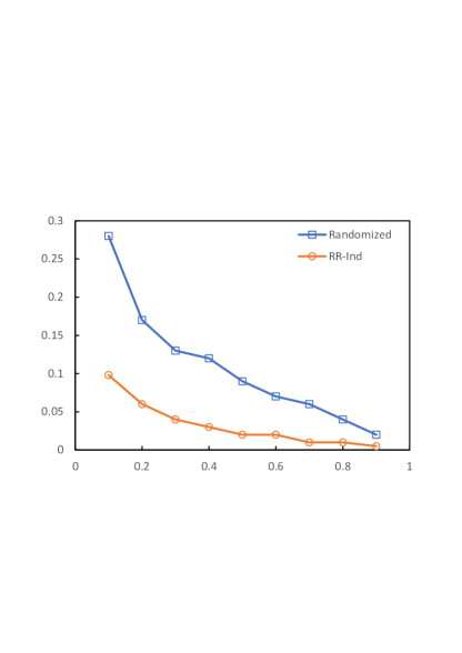
Figure 2: Absolute error (left) and relative error (right) of Randomized and RR-Independent when $p=0.7$. The $x$-axis represents the domain coverage $\sigma$.

The accuracy of estimations reported by RR-Clusters depends on the thresholds $T_{v}$ (maximum number of category combinations per cluster) and $T_{d}$ (minimum required dependence between attributes in a cluster), the actual data set and the randomization matrix used. Next, we analyzed the behavior of RR-Clusters for the Adult data set and for randomization matrices generated as per Section 6.3. In this evaluation, ${\bf S}$ was generated with $\sigma=0.1$. Table I shows the relative error of RR-Clusters for $T_{v}\in\{50,100,300\}$, $T_{d}\in\{0.1,0.2,0.3\}$ and a randomization matrix with $p\in\{0.1,0.3,0.5,0.7\}$. We observe that:

• As a rule, the relative error increased with $T_{v}$. This means that clusters with a high number of category combinations had a clear negative effect on the estimation accuracy.

• Regarding $T_{d}$, for small $p$ taking larger $T_{d}$ yielded better accuracy, whereas for larger $p$ taking smaller $T_{d}$ yielded better accuracy. Note that $T_{d}=0$ means that attributes can be clustered regardless of their dependence, whereas $T_{d}=1$ means that attributes are never clustered (in this case we have RR-Independent). Thus, clustering attributes turned out to be more rewarding for larger $p$, whereas for small $p$, there was less incentive for clustering and the advantage of RR-Clusters on RR-Independent was less noticeable.

TABLE I: Relative error of RR-Clusters in the Adult data set for $T_{v}\in\{50,100,300\}$, $T_{d}\in\{0.1,0.2,0.3\}$ and a randomization matrix with $p\in\{0.1,0.3,0.5,0.7\}$

			$T_{v}$
$p$	$T_{d}$	50	100	300
0.1	0.1	0.335	0.404	0.495
0.1	0.2	0.357	0.351	0.501
0.1	0.3	0.285	0.426	0.505
0.3	0.1	0.335	0.334	0.426
0.3	0.2	0.262	0.310	0.435
0.3	0.3	0.199	0.306	0.445
0.5	0.1	0.094	0.148	0.214
0.5	0.2	0.107	0.127	0.236
0.5	0.3	0.116	0.119	0.212
0.7	0.1	0.069	0.069	0.074
0.7	0.2	0.070	0.075	0.071
0.7	0.3	0.070	0.068	0.079

Next, we compared the accuracy of the methods listed in Section 6.2 for different levels of randomization ($p\in\{0.1,0.3,0.5,0.7\}$) and for different coverages of ${\bf S}$ ($\sigma\in\{0.1,0.2,0.3,0.4,$ $0.5,0.6,0.7,$ $0.8,0.9\})$. Figure 3 shows the relative error in the count queries. For each $p$, we took the best values for $T_{v}$ and $T_{d}$ identified in Table I. We observe that:

• For small values of $p$ (that is, for $p=0.1$ and $p=0.3$), RR-Independent yielded the best accuracy. For these values, using RR-Clusters and RR-Adjustment was counter-productive.

• For larger values of $p$ (that is, for $p=0.5$ and $p=0.7$) and large coverages ($\sigma\geq 0.3$) all methods behaved similarly and offered a very small relative error.

• For larger $p$ and small coverages ($\sigma<0.3$), RR-Clusters offered much more accuracy than RR-Independent. Furthermore, using RR-Adjustment brought a substantial accuracy improvement, no matter whether plugged after RR-Independent or RR-Clusters.

In summary, for strong randomization, the dependences between attributes in ${\bf X}$ are mostly lost in ${\bf Y}$. For this reason, in this case RR-Independent is as good as RR-Clusters, and RR-Adjustment does not bring much. In contrast, for weak randomization, it makes sense to leverage whatever dependences might be preserved in ${\bf Y}$, and thus RR-Clusters and RR-Adjustment outperform RR-Independent. This superior behavior is visible only for small coverages, because for large coverages the denominator of Expression (16) is so large that any method achieves a small relative error.

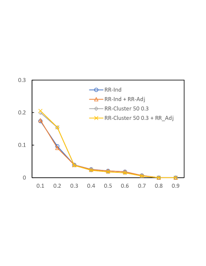
Figure 3: Relative error for different randomizations: $p=0.1$ (top left), $p=0.3$ (top right), $p=0.5$ (bottom left) and $p=0.7$ (bottom right). The $x$-axis represents the domain coverage $\sigma$.

Finally, we analyzed the effect of the data set size on the accuracy of the estimates. For the comparison with the previous results to be fair, we needed a data set with the same distribution. We obtained an expanded data set Adult6 by concatenating the original Adult data set 6 times. In this way, Table I for Adult became Table II for Adult6, which shows the relative error of RR-Clusters for $T_{v}\in\{50,100,300\}$, $T_{d}\in\{0.1,0.2,0.3\}$ and a randomization matrix with $p\in\{0.1,0.3,0.5,0.7\}$. By comparing Tables I and II we observe that the relative error decreased for all parameterizations but the reduction achieved depended on the specific parameterization. Specifically:

• For $p=0.7$, the reduction was small, because for so little randomization the relative error was already quite low in Table I. In this case, the highest reduction occurred for $T_{v}=300$, because Adult6 being larger than Adult, a larger number of category combinations had a lower negative impact on estimation accuracy. This highest reduction for $T_{v}=300$ caused the lowest relative error for $p=0.7$ to occur when $T_{v}=300$, which shows the advantages of allowing a great number of category combinations when the data set is sufficiently large.

• For smaller $p$ (that is, for higher randomization levels), the reduction in the relative error was more remarkable for $T_{v}=50$ and $T_{v}=100$. These thresholds on category combinations could be better accommodated using the larger data set Adult6. In contrast, allowing up to $T_{v}=300$ category combinations had an impact on the relative error that was compensated only partially by the increase in the data set size; hence, the reduction in the relative error for $p=0.1,0.3,0.5$ and $T_{v}=300$ was less spectacular than for lower $T_{v}$. Further, unlike for $p=0.7$, the highest $T_{v}$ did not achieve the lowest relative error: this seems to indicate that, as the randomization level increases, one needs larger data set sizes to be able to work with a great number of category combinations.

• The effect of the threshold $T_{d}$ on dependence did not seem to change with the data set size.

TABLE II: Relative error of RR-Clusters in the Adult6 data set for $T_{v}\in\{50,100,300\}$, $T_{d}\in\{0.1,0.2,0.3\}$ and a randomization matrix with $p\in\{0.1,0.3,0.5,0.7\}$

			$T_{v}$
$p$	$T_{d}$	50	100	300
0.1	0.1	0.189	0.312	0.459
0.1	0.2	0.173	0.310	0.449
0.1	0.3	0.183	0.339	0.462
0.3	0.1	0.149	0.202	0.369
0.3	0.2	0.171	0.225	0.376
0.3	0.3	0.178	0.217	0.369
0.5	0.1	0.080	0.084	0.123
0.5	0.2	0.082	0.075	0.126
0.5	0.3	0.083	0.079	0.127
0.7	0.1	0.064	0.066	0.056
0.7	0.2	0.064	0.066	0.057
0.7	0.3	0.065	0.065	0.060

7 Related work

Privacy preservation in data set releases has a substantial tradition in the statistics and computer science communities. Privacy models such as $k$-anonymity [24], $t$-closeness [20] and differential privacy [11], as well as many statistical disclosure control techniques [16], have been used to protect data sets before releasing them. All these works assume there is a trusted party that collects the true original data and takes care of protecting them.

Some attempts to enforce privacy models in a distributed manner have been made. For example, [25] proposed a way to enforce $k$-anonymity by promoting the collaboration between users. Also, local differential privacy has been proposed as an adaptation of differential privacy to the untrusted collector scenario. Most of the work in local differential privacy targets the distributed computation of data analytics. However, some well-known attempts to generate locally differentially private data sets have been made. For instance, RAPPOR [12] generates a data set that allows users to compute the frequencies of a given set of items. RAPPOR is based on randomized response and Bloom filters. An extension of RAPPOR is available that allows users to compute multivariate distributions [13]. While privacy models usually offer privacy guarantees at the record level (e.g. $k$-anonymity limits the chances of succesful re-identification of a record based on quasi-identifier attributes), attaining such guarantees becomes increasingly difficult as the number of attributes grows. This difficulty is serious in the trusted data collector scenario, and a fortiori in the more complex untrusted data collector scenario.

Some masking techniques can be applied locally by each individual before releasing her record (e.g. noise addition or generalization). However, the lack of a global view generally prevents adjusting the masking to the data set formed by all original individual records (e.g. to preserve covariances between attributes or to apply a stronger generalization to those values that are rare). In this context, randomized response is very convenient because despite being a local masking approach it allows the data collector to estimate the distribution of the original data. However, estimating the true original joint distribution is only feasible for a small number of attributes. For example, in [31] an approach is presented that starts with RR followed by estimation of the original distribution for a single binary attribute, then generalizes to a single multicategory attribute, and finally to several multicategory attributes (the case we deal with in this paper). However, the authors of [31] apply RR independently for each attribute, in a way similar to our RR-Independent protocol, which does not preserve the relations between the original attributes. Our proposal is to strike a compromise between dimensionality reduction and preservation of attribute relations by performing RR on clusters of attributes.

In [21], a method was proposed for clustering the attributes of high-dimensional data sets in view of mitigating the curse of dimensionality. The authors used hierarchical clustering algorithms to identify clusters of strongly correlated attributes. A substantial difference with our paper is that they considered the centralized anonymization paradigm, in which a data controller holds the entire original data set and can compute attribute dependences in a straightforward way. In contrast, we deal with local anonymization, in which the original record of each individual is only known to that individual.

An attribute clustering approach to allow randomized response of several attributes was presented in [10]. Unfortunately, this method requires non-negligible disclosure of original attributes to compute attribute dependences. Furthermore, it can yield large attribute clusters with too many category combinations and/or nearly independent attributes, which hampers accuracy. Our attribute clustering method is superior in several aspects: i) it does not cluster attributes unless the number of category combinations of the clustered attributes is below a certain threshold and unless the dependence between the clustered attributes is above a certain threshold; ii) it specifies three carefully crafted procedures to compute attribute dependences with minimum privacy loss for the individual parties; iii) our adjustment algorithm can partly compensate the accuracy lost by assuming independence between attributes in different clusters.

8 Conclusions and future research

Randomized response is an appealing anonymization approach in our big data era for several reasons. On the one side, it offers local anonymization and on the other side it can yield microdata useful for exploratory analysis and even machine learning. The main hindrance for using RR on multivariate data is the curse of dimensionality: as the number of attributes grows, the accuracy of the estimated distribution for the true original microdata quickly degrades.

In this paper, we have proposed mitigations to the dimensionality problem, based on performing RR separately for each attribute —which implicitly assumes all attributes are (nearly) independent— or jointly within clusters of attributes —which needs attributes in different clusters to be weakly dependent if not independent. We have then proposed a method to recover some of the estimation accuracy loss incurred by the above independence assumptions.

The proposed approaches open future research avenues. Randomized response assumes that all attributes are categorical or can be made categorical. Thus, a challenge is to devise local anonymization approaches yielding good distribution estimates for original numerical microdata with a large number of attributes. Another intriguing issue is whether there exist alternative ways to recover a larger share of the utility loss incurred by independence assumptions. Yet more daunting is to tackle a scenario in which all attributes are so correlated that any independence assumption will result in unaffordable accuracy loss.

Josep Domingo-Ferrer (Fellow, IEEE) is a distinguished professor of computer science and an ICREA-Acadèmia researcher at Universitat Rovira i Virgili, Tarragona, Catalonia, where he holds the UNESCO Chair in Data Privacy and leads CYBERCAT. He received the MSc and PhD degrees in computer science from the Autonomous University of Barcelona in 1988 and 1991, respectively. He also holds an MSc degree in mathematics. His research interests are in data privacy, data security and cryptographic protocols.

Jordi Soria-Comas is the Co-ordinator of Technology and Information Security at the Catalan Data Protection Authority, in Barcelona. He received an MSc in computer security (2011) and a PhD in computer science (2013) from Universitat Rovira i Virgili. He also holds an MSc in finance from the Autonomous University of Barcelona (2004) and a BSc in mathematics from the University of Barcelona (2003). His research interests are in data privacy and security.

References

- [1] S. Agrawal and J.R. Haritsa. A framework for high-accuracy privacy-preserving data mining. In ICDE’05 (2005) IEEE, pp. 193–204.
- [2] M. S. Alvim, K. Chatzikokolakis, C. Palamidessi and A. Pazii. Metric-based local differential privacy for statistical applications. CoRR abs/1805.01456 (2018).
- [3] M. Ben-Or, S. Goldwasser and A. Wigderson. Completeness theorems for non-cryptographic fault-tolerant distributed computation. In Proceedings of the 20th Annual ACM Symposium on Theory of Computing - STOC’88 (New York, NY, USA, 1988) ACM, pp. 1–10.
- [4] A. Chaudhuri and R. Mukerjee. Randomized response: theory and techniques. Marcel Dekker, 1988.
- [5] G. Cormode, S. Jha, T. Kulkarni, N. Li, D. Srivastava and T. Wang. and Wang, T. Privacy at scale: local differential privacy in practice. In SIGMOD 2018 (2018) ACM, pp. 1655–1658.
- [6] G. Cormode, T. Kulkarni and D. Srivastava. Marginal release under local differential privacy. In SIGMOD 2018 (2018) ACM, pp. 131–146.
- [7] H. Cramér. Mathematical Methods of Statistics. Princeton University Press, 1946.
- [8] T. Dalenius. Towards a methodology for statistical disclosure control. Statistik Tidskrift, 15 (1969) 429–444.
- [9] J. Domingo-Ferrer. Big data anonymization requirements vs privacy models. In 15th Intl. Conference on Security and Cryptography - SECRYPT 2018 (2018) pp. 471–478.
- [10] J. Domingo-Ferrer, R. Mulero-Vellido and J. Soria-Comas. Multiparty computation with statistical input confidentiality via randomized response. In Privacy in Statistical Databases - PSD 2018 (2018) Springer, pp. 175–186.
- [11] C. Dwork. Differential privacy. In Proceedings of the 33rd International Colloquium on Automata, Languages and Programming - ICALP 2006 (2006) Springer, pp. 1–12.
- [12] Ú. Erlingsson, V. Pihur and A. Korolova. RAPPOR: Randomized aggregatable privacy-preserving ordinal response. In Proc. of the 2014 ACM CCS SIGSAC Conference on Computer and Communications-CCS 2014 (2014) ACM, pp. 1054–1067.
- [13] G. Fanti, V. Pihur and Ú. Erlingsson. Building a RAPPOR with the unknown: privacy-preserving learning of associations and data dictionaries. In Proceedings on Privacy Enhancing Technologies, 3 (2016) 41–61.
- [14] S. L. Garfinkel, J. M. Abowd and S. Powazek. Issues encountered deploying differential privacy. In Proc. of the 2018 Workshop on Privacy in the Electronic Society-WPES 2018 (2018) ACM, pp. 133–137.
- [15] B. G. Greenberg, A.-L. A. Abul-Ela, W. R. Simmons and D. G. Horvitz. The unrelated question randomized response model: theoretical framework. Journal of the American Statistical Association, 64(326) (1969) 520–539.
- [16] A. Hundepool, J. Domingo-Ferrer, L. Franconi, S. Giessing, E. Schulte Nordholt, K. Spicer and P. P. de Wolf. Statistical Disclosure Control. Wiley, 2012.
- [17] P. Kairouz, S. Oh and P. Viswanath. Extremal mechanisms for local differential privacy. Journal of Machine Learning Research, 17(1) (2016) 492–542.
- [18] P. Kairouz, S. Oh and P. Viswanath. The composition theorem for differential privacy. IEEE Transactions on Information Theory 63(6) (2017) 4037–4049.
- [19] P. L. Kooiman, L. Willenborg and J. Gouweleeuw. PRAM: A Method for Disclosure Limitation of Microdata. Research Rep. 9705, Statistics Netherlands, Voorburg, NL, 1998.
- [20] N. Li, T. Li and S. Venkatasubramanian. t-Closeness: privacy beyond k-anonymity and l-diversity. In Proceedings of the 23rd IEEE International Conference on Data Engineering - ICDE 2007 (2007), IEEE, pp. 106–115.
- [21] A. Oganian, I. Iacob and G. Lesaja. Grouping of variables to facilitate SDL methods in multivariate data sets. In Privacy in Statistical Databases - PSD 2018 (2018) Springer, pp. 187–199.
- [22] W. Qardaji, W. Yang and N. Li. PriView: practical differentially private release of marginal contingency tables. In Proceedings of SIGMOD’14 (2014) ACM, pp. 1435–1446.
- [23] P. Rogaway. The moral character of cryptographic work. Invited talk at Asiacrypt 2015. IACR Cryptology ePrint Archive 2015 (2015), 1162.
- [24] P. Samarati and L. Sweeney. Protecting Privacy when Disclosing Information: -Anonymity and its Enforcement through Generalization and Suppression. SRI International report, 1998.
- [25] J. Soria-Comas and J. Domingo-Ferrer. Co-utile collaborative anonymization of microdata. In Modeling Decisions for Artificial Intelligence-MDAI 2015 (2015), pp. 192–206.
- [26] V. Strassen. Gaussian elimination is not optimal. Numerische Mathematik, 13(4) (1969) 354–356.
- [27] S. K. Thompson. Sample size for estimating multinomial proportions. The American Statistician, 41(1) (1987) 42–46.
- [28] A. van den Hout. Analyzing Misclassified Data: Randomized Response and Post Randomization. PhD thesis, University of Utrecht, 2004.
- [29] T. Wang, J. Blocki, N. Li and S. Jha. Locally differentially private protocols for frequency estimation. In Proceedings of the 26th USENIX Security Symposium (2017) ACM, pp. 729–745.
- [30] Y. Wang, X. Wu and D. Hu. Using Randomized Response for Differential Privacy Preserving Data Collection. Tech. rep. DPL-2014-003, University of Arkansas, 2014.
- [31] Y. Wang, X. Wu and D. Hu. Using randomized response for differential privacy preserving data collection. In Proceedings of the EDBT/ICDT 2016 Joint Conference (Bordeaux, France, 2016).
- [32] S. L. Warner. Randomized response: A survey technique for eliminating evasive answer bias. Journal of the American Statistical Association 60, 309 (1965), 63–69.
- [33] X. Zhang, L. Chen, K. Jin and X. Meng. Private high-dimensional data publication with junction tree. Journal of Computer Research and Development 55 (2018) 2794–2809.
- [34] J. Zhang, G. Cormode, C.M. Procopiuc, D. Srivastava and X. Xiao. PrivBayes: Private data release via Bayesian networks. ACM Transactions on Database Systems (TODS), 42(4) (2017) 1–41.
- [35] Z. Zhang, T. Wang, N. Li, S. He and J. Chen. CALM: Consistent adaptive local marginal for marginal release under local differential privacy. In Proceedings of the 2018 ACM SIGSAC Conference on Computer and Communications Security (CCS’18) (2018) ACM, pp. 212–229.