Tangent Quadrics in Real 3-Space

Abstract

We examine quadratic surfaces in $3$-space that are tangent to nine given figures. These figures can be points, lines, planes or quadrics. The numbers of tangent quadrics were determined by Hermann Schubert in 1879. We study the associated systems of polynomial equations, also in the space of complete quadrics, and we solve them using certified numerical methods. Our aim is to show that Schubert’s problems are fully real.

1 Introduction

There are $3264$ conics tangent to five given conics in the projective plane $\mathbb{P}^{2}$, and there exist five explicit conics so that all $3264$ complex solutions are real [2, 12]. We here study such tangency questions in one dimension higher. We consider quadrics (i.e. quadratic surfaces) in $\mathbb{P}^{3}$. Schubert [13] found that there are $666841088$ quadrics tangent to nine given quadrics in $\mathbb{P}^{3}$. Our ultimate goal is to decide whether there exist nine real quadrics so that all complex solutions are real. In this article we present first steps towards answering that question.

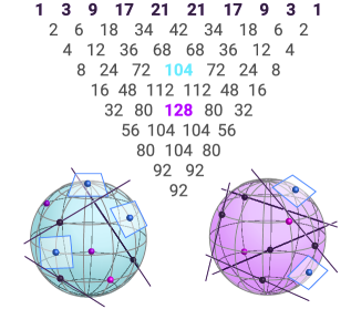
Figure 1: Schubert’s triangle for tangency of quadrics in 3-space.

Our study centers around Schubert’s triangle which is displayed in Figure 1. For each triple $(\alpha,\beta,\gamma)\in\mathbb{N}^{3}$ with $\alpha+\beta+\gamma=9$, the triangle shows the number $p^{\alpha}\ell^{\beta}h^{\gamma}$ of quadrics that pass through $\alpha$ given points, are tangent to $\beta$ given lines, and are tangent to $\gamma$ given planes. The two pictures, in blue and red, illustrate the geometric meaning of the entries $p^{3}\ell^{3}h^{3}={\color[rgb]{0,0,1}104}$ and $p^{2}\ell^{5}h^{2}={\color[rgb]{1,0,0}128}$.

Schubert derives these numbers in [13, §22]. In [13, page 106] he argues as follows. Quadrics degenerate into complete flags, consisting of a point on a line in a plane in $\mathbb{P}^{3}$. Such a flag counts with multiplicity two, since $q=2(p+\ell+h)$, by Proposition 2.4. We seek quadrics that satisfy one of the three tangency conditions, for each of the nine given flags. The number of such quadrics equals

$$q^{9}=\,\,2^{9}\!\!\!\!\!\sum_{\alpha{+}\beta{+}\gamma=9}\begin{matrix}\frac{9!}{\alpha!\beta!\gamma!}\end{matrix}\cdot p^{\alpha}\ell^{\beta}h^{\gamma}\,\,=\,\,2^{9}(\,\cdots+1680\cdot{\color[rgb]{0,0,1}104}+\cdots+756\cdot{\color[rgb]{1,0,0}128}+\cdots\,).\vspace{-0.07in}$$ (1)

The second equation is in the cohomology ring of the space of complete quadrics. In (1) we multiply each entry in Schubert’s triangle with the corresponding trinomial coefficient $\frac{9!}{\alpha!\beta!\gamma!}$, we add up the products, we multiply the sum by $2^{9}=512$, and we obtain $q^{9}=666841088$. This derivation is the analogue in $\mathbb{P}^{3}$ of the pentagon count for the $2^{5}(p+\ell)^{5}=3264$ conics in [2, Figure 3].

Schubert’s calculus predicts the number of complex solutions to a system of polynomial equations that depend on geometric figures like lines and planes in $\mathbb{P}^{3}$. In this article we study these polynomial equations and present practical tools for solving them. Our main interest is in solutions over the real numbers $\mathbb{R}$.

This paper is organized as follows. In Section 2 we introduce coordinates for points, lines, planes and quadrics, and derive the polynomials that describe our tangency conditions. Section 3 is dedicated to the space of complete quadrics, a variety in $\mathbb{P}^{9}\times\mathbb{P}^{20}\times\mathbb{P}^{9}$. We determine its prime ideal, we recover Schubert’s triangle as its multidegree, and we write our tangency conditions in that setting.

In Section 4 we argue that Schubert’s triangle is mostly real. We present explicit instances where all tangent quadrics are real. These instances were found by substantial computations using the software HomotopyContinuation.jl [3]. Our computations and the certification process are described in Section 5.

In Section 6 we turn to Schubert’s pyramid. It gives the numbers $p^{\alpha}\ell^{\beta}h^{\gamma}q^{\delta}$ of quadrics through $\alpha$ points that are tangent to $\beta$ lines, $\gamma$ planes and $\delta$ quadrics; see Figure 2. At the top of this pyramid lives $q^{9}=666841088$. We discuss the associated polynomial systems and we state two conjectures about their reality.

2 Coordinates and Equations

We begin with the coordinates that describe our geometric figures. A point $P$ in $\mathbb{P}^{3}$ is represented by a vector $p=(p_{1},p_{2},p_{3},p_{4})$. A line can be given by a $2\times 4$ matrix $L$, and a plane by a $3\times 4$ matrix $H$. We often use Plücker coordinates

$$\vspace{-0.04in}\ell=(\ell_{12},\ell_{13},\ell_{14},\ell_{23},\ell_{24},\ell_{34})\quad{\rm and}\quad h=(h_{234},-h_{134},h_{124},-h_{123}).$$

Here $\ell_{ij}$ is the $2\times 2$ minor of $L$ with column indices $i$ and $j$. Note the Plücker relation $\,\ell_{12}\ell_{34}-\ell_{13}\ell_{24}+\ell_{14}\ell_{23}=0$. Likewise $h_{ijk}$ denote the $3\times 3$ minors of $H$.

Remark 2.1.

Inclusion relations are written in Plücker coordinates as follows:

$$\begin{matrix}P\subset H:&&p_{1}h_{234}-p_{2}h_{134}+p_{3}h_{124}-p_{4}h_{123},\vskip 3.0pt plus 1.0pt minus 1.0pt\\ P\subset L:&&\begin{matrix}p_{1}\ell_{23}-p_{2}\ell_{13}+p_{3}\ell_{12}\,,\,\,p_{1}\ell_{24}-p_{2}\ell_{14}+p_{4}\ell_{12},\\ p_{1}\ell_{34}-p_{3}\ell_{14}+p_{4}\ell_{13}\,,\,p_{2}\ell_{34}-p_{3}\ell_{24}+p_{4}\ell_{23},\end{matrix}\vskip 3.0pt plus 1.0pt minus 1.0pt\\ L\subset H:&&\begin{matrix}\ell_{12}h_{134}-\ell_{13}h_{124}+\ell_{14}h_{123}\,,\,\,\ell_{12}h_{234}-\ell_{23}h_{124}+\ell_{24}h_{123},\\ \ell_{13}h_{234}-\ell_{23}h_{134}+\ell_{34}h_{123}\,,\,\,\ell_{14}h_{234}-\ell_{24}h_{134}+\ell_{34}h_{124}.\end{matrix}\end{matrix}$$

A triple $(P,L,H)$ satisfying $P\subset L\subset H$ is called a complete flag. The variety of complete flags is irreducible of dimension six in $\mathbb{P}^{3}\times\mathbb{P}^{5}\times\mathbb{P}^{3}$. The prime ideal of this flag variety is generated by the nine quadrics above, together with the Plücker relation. These ten generators form a Gröbner basis [11, Theorem 14.6].

Each quadric in $\mathbb{P}^{3}$ is represented by a symmetric $4\times 4$ matrix $X=(x_{ij})$. The point $P$ lies on the quadric $X$ if $PXP^{T}=0$. Similarly, the condition for $X$ to be tangent to a line $L$ or to a plane $H$ is given by the vanishing of the polynomial

$${\rm det}(LXL^{T})\,=\,\ell(\wedge_{2}X)\ell^{T}\quad{\rm or}\quad{\rm det}(HXH^{T})\,=\,h(\wedge_{3}X)h^{T}.$$ (2)

Here $\wedge_{i}X$ denotes the $i$-th exterior power of the $4\times 4$ matrix $X$. The entries of $\wedge_{i}X$ are the $i\times i$ minors of $X$. The rows and columns are labeled so that (2) holds.

Suppose we are given $\alpha$ points $P_{i}$, $\beta$ lines $L_{j}$, and $\gamma$ planes $H_{k}$, all generic, where $\alpha+\beta+\gamma=9$. We wish to solve these nine homogeneous equations for $X$:

$$\!P_{i}XP_{i}^{T}\,=\,{\rm det}(L_{j}XL_{j}^{T})\,=\,{\rm det}(H_{k}XH_{k}^{T})\,=\,0\,\,\,{\rm for}\,\,1\leq i\leq\alpha,\,1\leq j\leq\beta,\,1\leq k\leq\gamma.$$ (3)

Here $X$ is an unknown symmetric $4\times 4$ matrix, viewed as a point in $\mathbb{P}^{9}$, that satisfies ${\rm det}(X)\not=0$. Bézout’s Theorem suggests that the number of complex solutions to (3) equals $1^{\alpha}2^{\beta}3^{\gamma}$. This number is correct when $\alpha\geq 4$ and $\gamma\leq 2$. In all other cases, the equations (3) have extraneous solutions that are removed by saturation with respect to the ideal $\langle{\rm det}(X)\rangle$. This saturation step can be carried out in Macaulay2 [8]. For each choice of $(\alpha,\beta,\gamma)$, we obtain a Gröbner basis that reveals the number of solutions in $\mathbb{P}^{9}$. This computation proves the correctness of Schubert’s triangle. For solving (3) numerically, see Section 5.

We next discuss the condition for $X$ to be tangent to a fixed quadric $U=(u_{ij})$.

Lemma 2.2.

The condition for two quadrics $U$ and $X$ to be tangent in $\mathbb{P}^{3}$ is given by the discriminant of the quartic $f(t)={\rm det}(U+tX)$. This is an irreducible polynomial with $67753552$ terms of degree $(12,12)$ in the $20$ unknowns $u_{ij},\,x_{ij}$.

Proof 2.3.

The tangency condition means that the intersection curve of the quadrics $U$ and $X$ is singular in $\mathbb{P}^{3}$. By the Cayley trick of elimination theory [7, §3.2.D], this is singular if and only if the line spanned by $U$ and $X$ in $\mathbb{P}^{9}$ is tangent to the hypersurface $\{{\rm det}(X)=0\}$. That condition is given by the discriminant of $f(t)$, which is known as the Hurwitz form of $\{{\rm det}(X)=0\}$. We found its expansion into $67753552$ monomials with the computer algebra system Maple.

We denote the above discriminant by $\Sigma(U,X)$. If $U$ is a symmetric matrix with random entries in $\mathbb{R}$ or $\mathbb{C}$ then $\Sigma(U,X)$ is a polynomial of degree $12$ in ten unknowns $x_{ij}$ with $241592$ terms. Given nine quadrics $U_{1},\ldots,U_{9}$ in $\mathbb{P}^{3}$, the quadrics tangent to these solve the following equations in $\mathbb{P}^{9}$:

$$\Sigma(U_{1},X)\,=\,\Sigma(U_{2},X)\,=\,\,\cdots=\,\,\Sigma(U_{9},X)\,=\,0\quad{\rm and}\quad{\rm det}(X)\not=0.$$ (4)

Bézout’s Theorem suggests that the nine equations have $12^{9}$ complex solutions, but the inequation decreases that number to $q^{9}=666841088$. We derived this in the Introduction from Figure 1. A key ingredient was the identity $q=2(p+\ell+h)$.

We next prove this identity by an explicit geometric degeneration. Let $V$ be an invertible real $4\times 4$ matrix, and let $P\subset L\subset H$ be the flag given by its first three rows. We introduce a parameter $\epsilon>0$, and we consider the quadric defined by

$$U_{\epsilon}\,\,=\,\,V^{-1}\cdot{\rm diag}(\epsilon^{3},\epsilon^{2},\epsilon,1)\cdot(V^{-1})^{T}.$$ (5)

We investigate the behavior of the tangency condition for $U_{\epsilon}$ and $X$, as $\epsilon\rightarrow 0$.

Proposition 2.4.

The leading form in $\epsilon$ of the specialized Hurwitz form equals

$$\Sigma(U_{\epsilon},X)\,\,=\,\,(PXP^{T})^{2}\cdot\,{\rm det}(LXL^{T})^{2}\cdot\,{\rm det}(HXH^{T})^{2}\cdot\epsilon^{8}\,\,+\,\,\hbox{higher terms in $\epsilon$}.$$ (6)

This implies the identity $q=2(p+\ell+h)$ in the appropriate cohomology ring.

Proof 2.5.

The factorization in (6) can be seen directly from the discriminant of

$$f(t)\,=\,{\rm det}(U_{\epsilon}+tX)\,=\,c_{0}+c_{1}t+c_{2}t^{2}+c_{3}t^{3}+c_{4}t^{4}.$$

The coefficients $c_{i}$ are polynomials in $\epsilon$ with orders of vanishing $6,3,1,0,0$ at $\epsilon=0$. The discriminant has vanishing order $8$ at $\epsilon=0$, and this order is uniquely attained by its monomial $c_{1}^{2}c_{2}^{2}c_{3}^{2}$. The factors $c_{1},c_{2},c_{3}$ map to those in (6).

3 Complete Quadrics

A geometric setting for our tangency problems is the space of complete quadrics. By definition, this is the variety obtained as the closure of the image of the map

$$\mathbb{P}^{9}\,\,\dashrightarrow\,\,\mathbb{P}^{9}\times\mathbb{P}^{20}\times\mathbb{P}^{9}\,,\,\,\,\quad X\,\,\mapsto\,\,(X,\,\wedge_{2}X,\,\wedge_{3}X)\,\,\,=:\,\,\,(X,Y,Z).$$ (7)

Here $X=(x_{ij})$ and $Z=(z_{ijk,lmn})$ are symmetric $4\times 4$ matrices and $Y=(y_{ij,kl})$ is a symmetric $6\times 6$ matrix. The rows and columns of $Y$ and $Z$ are indexed just like the entries of $\ell$ and $h$. The $\mathbb{N}^{3}$-homogeneous ideal $\mathcal{I}_{4}$ of that $9$-dimensional variety lives in the polynomial ring $\mathbb{Q}[X,Y,Z]$ in $10+21+10=41$ unknowns.

Theorem 3.1.

The space of complete quadrics is a smooth variety of dimension nine. Its prime ideal $\mathcal{I}_{4}$ is minimally generated by $164$ polynomials, namely
$\bullet\,$ one linear form of degree $(010)$, i.e. $y_{12,34}-y_{13,24}+y_{14,23}$,
$\bullet\,$ $20$ quadrics of degree $(020)$, e.g. $y_{12,24}y_{24,34}-y_{13,24}y_{24,24}+y_{14,24}y_{23,24}$,
$\bullet$ $15$ quadrics of degree $(\!101\!)$, e.g. $x_{11}z_{123,234}-x_{12}z_{123,134}+x_{13}z_{123,124}-x_{14}z_{123,123}$,
$\bullet\,$ $64$ quadrics of degree $(011)$, e.g. $y_{12,13}z_{123,134}-y_{13,13}z_{123,124}+y_{13,14}z_{123,123}$,
$\bullet\,$ $64$ quadrics of degree $(110)$, e.g. $\,x_{11}y_{12,23}-x_{12}y_{12,13}+x_{13}y_{12,12}$.
Schubert’s triangle in Figure 1 equals the multidegree of $\,\mathcal{I}_{4}\,$ in the $\mathbb{N}^{3}$-grading.

Proof 3.2 (Proof).

The closure of the image of (7) is irreducible of dimension nine since $X$ appears in the first coordinate. The smoothness of this variety is well-known in the theory of spherical varieties. For a new perspective and proof see [10, §3.C].

The $164$ polynomials were found by computation using Macaulay2 [8]. To show that they generate the prime ideal $\mathcal{I}_{4}$, we use [6, Proposition 23] inductively. We eliminate one variable that occurs linearly in some equation and is not a zero-divisor modulo the current ideal. After checking these hypotheses, we replace the ideal by the elimination ideal, which is prime by induction. This process was found to work for various natural orderings of the entries in $X,Y,Z$.

The multidegree is a standard construction for multigraded commutative rings [11, Section 8.5]. For a variety in a product of projective spaces, it is the class of that variety in the cohomology ring of the ambient space. The built-in command multidegree in Macaulay2 takes only a few seconds to find the multidegree from our $164$ polynomials. The output of this Macaulay2 computation is a ternary form in the unknowns $T_{0},T_{1},T_{2}$. It has $55$ terms of degree ${\rm codim}(\mathcal{I}_{4})=29$. The coefficient of $T_{0}^{9-\alpha}T_{1}^{20-\beta}T_{2}^{9-\gamma}$ is the number $p^{\alpha}\ell^{\beta}h^{\gamma}$ in Figure 1. This computation is an ab initio derivation of Schubert’s triangle.

The variety $V(\mathcal{I}_{4})$ captures degenerations of quadrics that matter in intersection theory [10]. We saw this in Proposition 2.4 where the quadric becomes a flag $P\subset L\subset H$. The relationship to the flag variety is made precise as follows:

Corollary 3.3.

The variety of complete flags in $\mathbb{P}^{3}$ is the inverse image of $V(\mathcal{I}_{4})$ under the componentwise Veronese embedding $\,\mathbb{P}^{3}\times\mathbb{P}^{5}\times\mathbb{P}^{3}\,\hookrightarrow\,\mathbb{P}^{9}\times\mathbb{P}^{20}\times\mathbb{P}^{9}$.

Proof 3.4.

The Veronese map takes $(p,\ell,h)$ to the rank one matrices $(X,Y,Z)=(p^{T}p,\,\ell^{T}\ell,\,h^{T}h)$. Substituting this into $\mathcal{I}_{4}$ and saturating by the irrelevant ideal of $\mathbb{P}^{3}\times\mathbb{P}^{5}\times\mathbb{P}^{3}$ yields the Gröbner basis for the flag variety in Remark 2.1.

We next lift our tangency conditions from the space $\mathbb{P}^{9}$ of symmetric matrices $X$ to the space of complete quadrics in $\mathbb{P}^{9}\times\mathbb{P}^{20}\times\mathbb{P}^{9}$. We write $\,\mathcal{B}\,=\,\langle X\rangle\,\cap\,\langle Y\rangle\,\cap\,\langle Z\rangle\,$ for the irrelevant ideal of that product of projective spaces.

The condition that a quadric contains a point $p$ is the linear form $pXp^{T}$ in the unknown $X$. Similarly, tangency to a line $\ell$ is the linear form $\ell\,Y\ell^{T}$ in the unknown $Y$, and tangency to a plane $h$ is the linear form $hZh^{T}$ in the unknown $Z$. Without loss of generality, we can assume that one given figure is a coordinate subspace in $\mathbb{P}^{3}$. Then the three linear forms are variables $x_{11}$, $y_{12,12}$ or $z_{123,123}$.

However, if we augment $\mathcal{I}_{4}$ by one such variable then the resulting ideal is not prime. To get the correct prime ideal we must saturate by the irrelevant ideal $\mathcal{B}$. We first summarize what happens when we add the constraint for a point. The result is the same for the plane constraint if we swap the roles of $X$ and $Z$.

Proposition 3.5.

The saturation $\bigl{(}(\mathcal{I}_{4}+\langle x_{11}\rangle):\mathcal{B}^{\infty}\bigr{)}$ is the prime ideal of the variety of complete quadrics that contain a given point. It has $13$ minimal generators in addition to the $164$ generators of $\mathcal{I}_{4}$, namely ten of degree $(020)$ and one each of degree $(100)$, $(003)$ and $(011)$. The multidegree of this ideal is the triangle of size eight that is obtained by deleting the lower right edge in Figure 1.

Proof 3.6.

This is proved by a Macaulay2 computation. The new equation of degree $(100)$ is $x_{11}$. The new equation of degree $(003)$ is the complementary $3\times 3$ minor of $Z$. Generators of degree $(020)$ arise from Bareiss formula which says that $x_{11}$ times any $3\times 3$ minor of $X$ containing $x_{11}$ equals a $2\times 2$ minor of $Y$.

Proposition 3.7.

The saturation $\bigl{(}(\mathcal{I}_{4}+\langle y_{12,12}\rangle):\mathcal{B}^{\infty}\bigr{)}$ is the prime ideal for the complete quadrics that are tangent to a line. It has three minimal generators, of degrees $(010),(200),(002)$, in addition to the $164$ generators of $\mathcal{I}_{4}$. This is one entry of $Y$ and the corresponding $2\times 2$ minors of $X$ and $Z$. The multidegree is the triangle of size eight obtained by deleting the top edge in Figure 1.

It would be desirable to extend Theorem 3.1 to $n\times n$ matrices for $n\geq 5$, i.e. to identify minimal generators for the multihomogeneous prime ideal of the space of complete quadrics. These are relations among all minors of a symmetric $n\times n$ matrix that respect the fine grading coming from the size of the minors. Results by Bruns et al. [4] indicate that relations of degree $\leq 2$ will not suffice.

4 Schubert’s Triangle

At present, we have the following result on the reality of Schubert’s triangle.

Theorem 4.1.

For at least $46$ of the $55$ problems in Schubert’s triangle, there exists an open set of real instances, consisting of $\alpha$ points, $\beta$ lines and $\gamma$ planes, such that all complex solutions in $\mathbb{P}^{9}$ to the polynomial equations in (3) are real. For the other nine problems, the current status is summarized in Remark 4.3.

Example 4.2.

Fix $(\alpha,\beta,\gamma)=(3,3,3)$. We consider the configuration

$$\begin{matrix}p&=&(1,\frac{439}{922},-\frac{347}{271},\frac{67}{343})\,,\,\,(1,-\frac{211}{484},\frac{153}{346},\frac{257}{254})\,,\,\,(1,-\frac{575}{404},\frac{131}{320},-\frac{37}{42}),\vskip 6.0pt plus 2.0pt minus 2.0pt\\ \ell&=&(-\frac{92}{159},-\frac{92}{293},\frac{120}{307},\frac{77}{256},\frac{76}{391},\frac{96}{311})\,,\,\,(\frac{107}{114},\frac{18}{383},-\frac{109}{116},\frac{37}{217},\frac{45}{307},\frac{47}{264})\,,\,\,\vskip 6.0pt plus 2.0pt minus 2.0pt\\ &&(-\frac{365}{302},-\frac{45}{368},\frac{172}{209},\frac{74}{245},\frac{25}{62},\frac{87}{353}),\vskip 6.0pt plus 2.0pt minus 2.0pt\\ h&=&(\frac{193}{182},\frac{75}{397},-\frac{244}{631},\frac{195}{272})\,,\,\,(\frac{91}{307},-\frac{17}{122},-\frac{553}{837},\frac{70}{309})\,,\,\,(\frac{919}{295},\frac{103}{36},\frac{1199}{371},\frac{57}{176}).\end{matrix}$$

All $104$ complex quadrics tangent to these nine figures are found to be real. Thus, this is a fully real instance for the scenario shown in blue in Figure 1.

Remark 4.3.

Up to the natural involution, given by swapping points and planes, there are $30$ distinct tangency problems in Schubert’s triangle. For five of the problems we have not yet succeeded in verifying reality. They are as follows:

$$\begin{matrix}(\alpha,\beta,\gamma)&\!\!&(3,4,2)&(3,5,1)&(2,6,1)&(1,7,1)&(1,8,0)\\ \!\hbox{Schubert's count over $\mathbb{C}$}&\!\!&112&80&104&104&92\\ \hbox{Our current record over $\mathbb{R}$}&\!\!&110&74&96&84&84\\ \end{matrix}$$

For instance, we know two points, six lines and a plane in $\mathbb{P}^{3}_{\mathbb{R}}$ such that $96$ real quadrics are tangent to these figures. The remaining eight quadrics are complex. This is derived from Example 4.5 by replacing point $P_{3}$ with a plane. For the (1,8,0) case with $84$ real solutions we use eight tangent lines as in Example 4.7.

Proof 4.4 (Discussion and proof of Theorem 4.1).

All our instances of full reality or maximal reality, along with the software that certifies correctness, can be found at

$$\href https://mathrepo.mis.mpg.de/TangentQuadricsInThreeSpace/index.html$$ (8)

For instance, for $(\alpha,\beta,\gamma)=(3,3,3)$, this website contains the configuration in Example 4.2, along with the $104$ tangent quadrics. Each quadric is determined by its nine points of tangency. The coordinates of these points form a $104\times 9\times 4$ tensor of floating point numbers in Julia format. The proof of correctness was carried out with the certification technique in [1], as discussed in Section 5.

We now present some ideas that were helpful in creating fully real instances. Figures given by the standard basis $e_{1},e_{2},e_{3},e_{4}$ lead to sparse equations in (3).

Example 4.5.

The condition for $X$ to be tangent to the six coordinate lines is

$$I\,\,=\,\,\langle\,x_{ii}x_{jj}-x_{ij}^{2}\,:\,1\leq i<j\leq 4\,\rangle.$$ (9)

This is the complete intersection of eight prime ideals, each isomorphic to the ideal $J$ generated by all $2\times 2$ minors of $X$. The eight primes are $\,U_{ijk}\star J$, where $\star$ is the Hadamard product, and $U_{ijk}$ is the $4\times 4$ matrix with entries $(-1)^{i}$, $(-1)^{j}$ and $(-1)^{k}$ in positions $(2,3)$, $(2,4)$ and $(3,4)$, and entries $1$ everywhere else. Seven of these scaled Veronese varieties contain matrices of rank $3$ or $4$. Their union is defined by the radical ideal $(I:J)$, which has degree $56$. This is Schubert’s number for $\alpha=3,\beta=6,\gamma=0$. We seek three points such that all $56$ quadrics containing these and satisfying $I$ are real. One choice that works is

$$P_{1}=(1,2,8,7),\quad P_{2}=(1,1,9,2),\quad P_{3}=(2,5,3,1).$$

Our six given lines meet pairwise, and they are not generic. This leads to $48$ of the $56$ quadrics being cones. To get $56$ smooth quadrics, one perturbs the lines.

We refer to the article [9] by Kahle and Wagner for a general study of the ideal of principal $2\times 2$ minors of a symmetric $n\times n$ matrix of unknowns. Their results elucidate the decomposition we found for the special case $n=4$ in (9).

Example 4.6.

The condition for $X$ to be tangent to the four coordinate planes is the ideal generated by the four principal $3\times 3$ minors. Saturating by the ideal of all $3\times 3$ minors yields a prime ideal $K$ of codimension $4$ and degree $21$. This is Schubert’s number for $\alpha=5,\beta=0,\gamma=4$. It is easy to find five points so that all $21$ quadrics containing these and satisfying $K$ are real. This instance is generic.

The ideal $K$ is generated by $10$ cubics and $12$ quartics. The $5$-dimensional variety cut out by $K$ in $\mathbb{P}^{9}$ has the following nice parametric representation:

$$\small X\,=\,\begin{pmatrix}x_{12}x_{13}x_{14}\!\!\!\!&\!\!x_{12}\!\!&\!\!x_{13}\!\!&\!\!x_{14}\\ x_{12}\!\!&\!\!\!\!\!x_{12}x_{23}x_{24}\!\!\!\!&\!\!\!x_{23}\!\!&\!\!x_{24}\\ x_{13}\!\!&\!\!x_{23}\!\!&\!\!\!\!\!x_{13}x_{23}x_{34}\!\!\!\!&\!\!x_{34}\\ x_{14}\!\!&\!\!x_{24}\!\!&\!\!x_{34}\!\!&\!\!\!\!\!x_{14}x_{24}x_{34}\end{pmatrix}\,\,\,\,{\rm where}\,\,\,\,{\rm det}\begin{pmatrix}x_{12}x_{34}\!\!\!\!&\!\!1\!\!&\!\!1\\ 1\!\!&\!\!\!\!x_{13}x_{24}\!\!\!\!&\!\!1\\ 1\!\!&\!\!1\!\!&\!\!\!\!x_{14}x_{24}\end{pmatrix}=0.$$

Our final technique was inspired by the solution to Shapiro’s conjecture [14].

Example 4.7.

Consider the lines $\ell=(1,2t,3t^{2},t^{2},2t^{3},t^{4})$ that are tangent to the twisted cubic curve $\{(1:t:t^{2}:t^{3})\}$. There is a surface of quadrics tangent to all such lines. We choose nine nearby lines, by slightly perturbing nine tangent lines. Our fully real instance for $(\alpha,\beta,\gamma)=(0,9,0)$ was found in this manner.

5 Numerical Methods

We now explain our techniques for solving the equations (3) and for certifying the correctness of their solutions. Each instance is presented in the Plücker coordinates of Remark 2.1. Following (2) and Section 3, each line specifies a linear equation in $Y=\wedge_{2}X$ and each plane gives a linear equation in $Z=\wedge_{3}X$.

The numerical software HomotopyContinuation.jl due to Breiding and Timme [2, 3] is easy to use, even for those who are not yet familiar with julia. We now go over our steps in solving the system for the instance in Example 4.2.

The input is a system of $11$ equations in $11$ unknowns, namely the ten entries of the matrix $X$ and one more variable $D$. One equation is $D=\det(X)$, another specifies a random affine chart, $\sum_{1\leq i<j\leq 4}c_{ij}x_{ij}=1$, and the others are the tangency conditions. Our equations are entered into  HomotopyContinuation.jl:

Equations=System(vcat(Point_Conditions,                       Line_Conditions,                       Plane_Conditions,                       det(X)-D, Affine_Chart))

After entering  S=solve(Equations), the following output appears:

Tracking 216 paths... 100% |||||||||||||||| Time: 0:00:11 # paths tracked:                  216 # non-singular solutions (real):  104 (104) # singular endpoints (real):      84 (83) # total solutions (real):         188 (187)

This suggests that the program tracked $216=1^{\alpha}2^{\beta}3^{\gamma}$ paths from a total degree start system and that it found $104$ real nonsingular solutions. The variable S is a $104$-element array of solutions, each of which is an $11$-element array of floating point numbers. The first coordinate is D, and the last ten are the coordinates of X.

The following code extracts the $17$-th element of S and prints that quadric:

quadric=solutions(S)[17] @var x[1:4] Quadric=expand(x’*(X(Equations.variables=>real(quadric)))*x) -2.974732003076*x2*x1-1.289476735251*x2*x3-10.97658863786*x3*x1+ +8.372046844711*x4*x1+8.886907306683*x4*x2+9.704839838537*x4*x3+ -5.810893956281*x1^2+2.645663598009*x2^2-5.046922439351*x3^2+0.6937980589394*x4^2

These julia fragments give a first impression. The details may be found at (8).

One key question about numerical output is whether it can serve as a mathematical proof. How can we be sure that the $104$ solutions are indeed solutions and moreover, that they are distinct, real, and nondegenerate? This is addressed by the process of a-posteriori certification, which generates an actual proof.

We carry this out using the Krawczyk method, implemented by Breiding, Rose and Timme [1]. It is based on interval arithmetic and is now available as a standard feature in HomotopyContinuation.jl. We note that this implementation represents a significant advance over Smale’s $\alpha$-certification that was used for the $3264$ real quadrics in [2, Proposition 1]. This advance has two aspects. First, the new method in [1] is much faster. Second, its output gives a bounding box, allowing us to easily certify that the quadrics are nondegenerate.

We now show how certification works for our instance. The input is easy:

C=certify(Equations,S)

The program creates a certificate C, and it reports on that as follows:

CertificationResult =================== • 104 solutions given • 104 certified solutions (104 real) • 104 distinct certified solutions (104 real)

The certificate C is a list of $104$ lists of $22$ intervals $I_{1},\ldots,I_{11},J_{1},\ldots,J_{11}$ in $\mathbb{R}$. The product $B=\prod_{i=1}^{11}(I_{i}+\texttt{im}\cdot J_{i})$ is a box in $\mathbb{C}^{11}\simeq\mathbb{R}^{22}$. That box provably contains a unique solution to Equations, verified by interval arithmetic.

Checking that these boxes are disjoint proves that the $104$ solutions are distinct. Checking that $B$ is the only box which intersects the complex conjugate of $B$ itself proves that this solution is real. Checking that $0$ is not contained in $I_{1}$, the interval for the unknown D proves that the quadric is nondegenerate.

The following command displays the certifying box $B$ for the $17$-th quadric:

C.certificates[17].certified_solution (1.459827495775684e-6 ± 2.2938e-14) + (0.0 ± 2.2938e-14)im (-0.9684823260468921 ± 1.516e-09) + (0.0 ± 1.516e-09)im (-0.24789433358973637 ± 2.2975e-11) + (0.0 ± 2.2975e-11)im (0.44094393300164797 ± 1.1016e-09) + (0.0 ± 1.1016e-09)im (-0.9147157198219121 ± 1.3088e-09) + (0.0 ± 1.3088e-09)im (-0.10745639460424983 ± 3.3522e-10) + (0.0 ± 3.3522e-10)im (-0.8411537398918771 ± 1.0251e-09) + (0.0 ± 1.0251e-09)im (0.6976705703926359 ± 9.7633e-10) + (0.0 ± 9.7633e-10)im (0.7405756088903332 ± 1.1508e-09) + (0.0 ± 1.1508e-09)im (0.8087366532114602 ± 1.202e-09) + (0.0 ± 1.202e-09)im (0.11563300982325174 ± 7.2217e-10) + (0.0 ± 7.2217e-10)im

Remark 5.1.

Finding the fully real instances for Theorem 4.1 was a challenge. We implemented a heuristic hill-climbing algorithm similar to the one in [5]. The idea is to begin at some configuration $\mathcal{C}$ of $\alpha$ real points, $\beta$ real lines, and $\gamma$ real planes, solve the equations, and sample many nearby instances. If one has more real solutions, then $\mathcal{C}$ is updated to be that instance. Otherwise, the new $\mathcal{C}$ is the instance with the same number of real solutions, but whose complex solutions are closest to becoming real. This is measured by the minimum norm of the complex parts of each nonreal solution. In this fashion, one greedily travels through the parameter space towards instances with more real solutions. A major issue with such methods is that they get stuck in local maxima. Our success came from many iterations beginning at different randomly chosen parameters. A host of numerical tolerances determine the behavior of this algorithm. Once the number of real solutions approaches the maximum, the instances often become so ill-conditioned that serious monitoring of these tolerances is required.

6 Schubert’s Pyramid

We now finally come to the analogue in $\mathbb{P}^{3}$ of the number $3264$. The following conjecture motivated this project. We hope that it can be resolved in the future.

Conjecture 6.1.

There exist nine quadrics in $\mathbb{P}^{3}_{\mathbb{R}}$ such that all $666841088$ complex quadrics that are tangent to these nine are defined over the real numbers $\mathbb{R}$.

We propose a combinatorial gadget for approaching this problem. Schubert’s pyramid is a tetrahedron of $220$ intersection numbers $p^{\alpha}\ell^{\beta}h^{\gamma}q^{\delta}$, where $(\alpha,\beta,\gamma,\delta)\in\mathbb{N}^{4}$ with $\alpha+\beta+\gamma+\delta=9$. Here $q=2(p+\ell+h)$ denotes the cohomology class of the complete quadrics tangent to a given quadric in $\mathbb{P}^{3}$. Thus the pyramid organizes the number of quadrics tangent to nine figures, as in Figure 2.

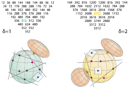
Figure 2: Two consecutive levels in Schubert’s pyramid

The levels in Schubert’s pyramid are the triangles for fixed $\delta$. Each entry in level $\delta$ is twice the sum of the three entries in level $\delta-1$ that lie below it. For instance, for $\delta=2$ we marked $3712=2\cdot(576+576+704)$. This counts quadrics through two points that are tangent to three lines, two planes and two quadrics.

Making Schubert’s triangle fully real is only a first step towards Conjecture 6.1. What we really want is to find one single instance of nine real flags:

$$P_{1}\subset L_{1}\subset H_{1}\,,\,\,P_{2}\subset L_{2}\subset H_{2}\,,\,\ldots\,,\,\,P_{9}\subset L_{9}\subset H_{9}.$$ (10)

We want those nine flags to exhibit full reality, simultaneously for all their many tangency problems. Such a configuration (10) would be the $3$-dimensional analogue to the pentagon in [2, Figure 3]. To state this precisely, we consider an arbitrary function $\psi:\{1,2,\ldots,9\}\rightarrow\{P,L,H\}$. This defines a polynomial system

$${\rm det}\bigl{(}\psi(i)_{i}\cdot X\cdot\psi(i)_{i}^{T}\bigr{)}\,=\,0\quad{\rm for}\,\,\,\,i=1,2,\ldots,9.$$ (11)

This has the form (3), where $\alpha=|\psi^{-1}(P)|$, $\beta=|\psi^{-1}(L)|$, and $\gamma=|\psi^{-1}(H)|$. Thus, an instance (10) of nine flags gives a collection of $3^{9}$ polynomial systems. For each of these, the number of solutions is one entry in Schubert’s triangle.

Conjecture 6.2.

There exist nine real flags (10) in $\mathbb{P}^{3}$ such that each complex solution $X$ to any of the $3^{9}$ associated polynomial systems (11) is a real quadric.

If Conjecture 6.2 is true, then we can approach Conjecture 6.1 as follows. We are given $\,(p+\ell+h)^{9}=1302424$ real quadrics $X$ that solve the $3^{9}$ systems. Each solution becomes $2^{9}$ distinct solutions under the deformation in Proposition 2.4, where the nine flags for $\epsilon=0$ become nine smooth quadrics for $\epsilon>0$.

This process can be performed in stages, from the bottom to the top of the pyramid, but its numerical implementation will not be easy. One hope is that reality can be controlled using the results by Ronga, Tognoli and Vust in [12].

Acknowledgements. We thank Sascha Timme for his important contributions.

References

- [1] P. Breiding, K. Rose and S. Timme: Certifying roots of polynomial systems using interval arithmetic, arXiv:2011.05000.
- [2] P. Breiding, B. Sturmfels and S. Timme: 3264 Conics in a Second, Notices of the American Mathematical Society 67 (2020) 30–37.
- [3] P. Breiding and S. Timme: HomotopyContinuation.jl: A package for homotopy continuation in Julia, Mathematical Software, ICMS 2018, Lecture Notes in Computer Science, 10931 (2018) 458-465.
- [4] W. Bruns, A. Conca and M. Varbaro: Relations between the minors of a generic matrix, Advances in Mathematics 244 (2013) 171–206.
- [5] P. Dietmaier: The Stewart-Gough platform of general geometry can have 40 real postures, J. Lenarčič, M.L. Husty (eds): Advances in Robot Kinematics: Analysis and Control, 7–16, Springer, Dordrecht, (1998).
- [6] L. Garcia, M. Stillman and B. Sturmfels: Algebraic geometry of Bayesian networks, Journal of Symbolic Computation 39 (2005) 331–355.
- [7] I.M. Gel’fand, M.M. Kapranov and A.V. Zelevinsky: Discriminants, Resultants and Multidimensional Determinants, Birkhäuser, Boston (1994).
- [8] D. Grayson and M. Stillman: Macaulay2, a software system for research in algebraic geometry, available at http://www.math.uiuc.edu/Macaulay2/.
- [9] T. Kahle and A. Wagner: Veronesean almost binomial almost complete intersections, Rend. Istit. Mat. Univ. Trieste 50 (2018) 75–79.
- [10] M. Michałek, L. Monin and J. Wiśniewski: Maximum likelihood degree, complete quadrics and -action, SIAM Journal on Applied Algebra and Geometry (2021).
- [11] E. Miller and B. Sturmfels: Combinatorial Commutative Algebra, Graduate Texts in Mathematics, Springer Verlag, New York, (2004).
- [12] F. Ronga, A. Tognoli and T. Vust: The number of conics tangent to five given conics: the real case, Rev. Mat. Univ. Complut. Madrid 10 (1997) 391–421.
- [13] H. Schubert: Kalkül der abzählenden Geometrie, Reprint of the 1879 original, Springer, Berlin, (1979).
- [14] F. Sottile: Frontiers of reality in Schubert calculus, Bulletin of the American Mathematical Society 47 (2010) 31–71.