MonoComb: A Sparse-to-Dense Combination Approach for Monocular Scene Flow

Abstract.

Contrary to the ongoing trend in automotive applications towards usage of more diverse and more sensors, this work tries to solve the complex scene flow problem under a monocular camera setup, i.e. using a single sensor. Towards this end, we exploit the latest achievements in single image depth estimation, optical flow, and sparse-to-dense interpolation and propose a monocular combination approach (MonoComb) to compute dense scene flow. MonoComb uses optical flow to relate reconstructed 3D positions over time and interpolates occluded areas. This way, existing monocular methods are outperformed in dynamic foreground regions which leads to the second best result among the competitors on the challenging KITTI 2015 scene flow benchmark.

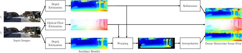
Figure 1. Overview of our pipeline for monocular dense scene flow estimation.

A block diagram showing the structure and data flow of the proposed approach.

1. Introduction

One current trend for many applications in assisted or autonomous driving is the utilization and fusion of as many sensors as available. As a result, certain approaches have increasing requirements on the hardware in a product. A different strategy is to solve the same problems based on input from less sensors, which allows to have the same functionality at lower cost. This becomes possible by adding constraints or assumptions to the formulation of the problem, by technical progress, or by relying on more or other visual cues.

In this work, the problem at hand is the estimation of dense 3D scene flow. Scene flow can be considered the 3D equivalent of 2D optical flow, which is achieved by additional 3D reconstruction of the scene. In most conventional approaches, a pair (or sequence) of stereo images is used as input. The stereo view allows for the 3D reconstruction, while the images at different points in time provide a motion cue and the temporal information. Recently, methods that operate solely on point clouds from LiDAR sensors were proposed (Liu et al., 2019; Behl et al., 2019). These approaches however are less dense compared to the standard resolution of images. Therefore, the fusion of cameras and LiDAR have been considered, either in the stereo case (Battrawy et al., 2019) or in the monocular case (Rishav et al., 2020), where the LiDAR measurements replace the stereo dependency for 3D reconstruction.

However, following the strategy to reduce the sensor input, we propose a method to estimate scene flow in the purely monocular case. While a single RGB camera does not provide a geometric cue as in stereo cameras and is also unable to measure depth directly as a LiDAR or RGB-D camera is, this setup poses scene flow estimation as a much more difficult problem. To our rescue, latest developments in single image depth estimation have proven that absolute depth can be reconstructed from a single view point (Godard et al., 2017; Fu et al., 2018; Godard et al., 2019; Ochs et al., 2019; Lee et al., 2019). This is possible by relying on depth cues like the monocular motion parallax, defocus blur by the field of depth, linear perspective, texture gradients, or the relative size of known objects.

We exploit the progress in the field of single image depth estimation and use it within the combination framework for scene flow (Schuster et al., 2018a) where geometry and temporal image correspondences are estimated separately and are later combined to obtain full 3D scene flow. Towards that end, we propose to 1.) estimate depth from two single images, 2.) estimate optical flow between these two images, 3.) correlate corresponding 3D points to estimate 3D motion, and 4.) interpolate gaps due to occlusions to obtain a dense result. The overview of these steps is given in Figure 1. Since our combination approach operates in a monocular camera setting, we term the proposed method MonoComb.

2. Related Work

In the very beginning of scene flow estimation the problem has already been formulated for a monocular camera (Vedula et al., 2005), however with a strong dependency on multiple views. Shortly after, stereo cameras were used to provide a better geometric cue for depth estimation (Huguet and Devernay, 2007; Wedel et al., 2008; Vogel et al., 2013). A parallel evolution was using RGB-D cameras to measure the geometry of the scene directly (Herbst et al., 2013; Hornacek et al., 2014). As mentioned earlier, the emerging use of laser scanners in vehicles has driven the development of scene flow algorithms in the point cloud domain (Liu et al., 2019; Behl et al., 2019; Wang et al., 2020). And lastly, camera and LiDAR information has been fused to solve the problem of scene flow estimation (Battrawy et al., 2019; Rishav et al., 2020).

Opposed to all these methods, our work presents a method to estimate scene flow from just two consecutive images from a monocular camera. There are a few approaches considering the same setup. In Mono-SF (Brickwedde et al., 2019), pixel-wise depth distributions are estimated for both images and then used in a probabilistic optimization framework to estimate rigidly moving, planar segments for the scene. Though the superpixel segmentation provides a strong regularization and high accuracy, the assumptions of rigidity and planarity introduce errors depending on the granularity of the segmentation. Also, the optimization is computational heavy. Self-Mono-SF (Hur and Roth, 2020) uses an adaptation of PWC-Net (Sun et al., 2018) that is trained in an self-supervised manner to jointly estimate 3D position and 3D flow at a quarter resolution. This methods is able to achieve competitive results after supervised fine-tuning, but the purely unsupervised version lags behind. Lastly, OpticalExpansion (OE) (Yang and Ramanan, 2020) exploits the assumption that most of the change of the projected size of objects is due to the change in distance to the observer. Therefore the authors argue that the relative motion-in-depth can be estimated directly together with optical flow. In conjunction with an estimate for the depth in one frame, the depth at the second frame can be reconstructed to obtain full scene flow.

Since most of the previous work in monocular scene flow estimation – as well as our proposed approach – rely on single image depth estimation, we discuss a part of state-of-the-art in this area as well. LRC (Godard et al., 2017) is a self-supervised approach that uses an encoder-decoder network architecture and trains with a photometric loss and consistency between left and right view of a stereo camera. The approach was later refined in MonoDepth2 (Godard et al., 2019). DORN (Fu et al., 2018) proposes to use a ordinal regression loss instead of a regular regression loss to train a network for single image depth estimation. This formulation is closer to monocular depth cues, where it is often easier to order the depth of regions instead of regressing the absolute depth of each point. BTS (Lee et al., 2019) represents state-of-the-art across different data sets. The idea of BTS is to fuse depth estimates from multiple scales at full resolution using local planar guidance for up-sampling.

Finally, very related work is the combination approach for stereo scene flow estimation in (Schuster et al., 2018a, b). Though the sensor setup is different from ours, the ideas are similar: Separate the complex problem of scene flow estimation into several (solved) sub-problems. In the work by (Schuster et al., 2018a), this concept yields non-dense scene flow, due to occlusion. The work of (Schuster et al., 2018b) solved this limitation by applying the interpolation method of SceneFlowFields (Schuster et al., 2018c) to the non dense result. Since our objective is dense scene flow as well, we also apply an interpolation method to fill in the gaps after warping. However in contrast to these previous approaches, our initial depth estimates are obtained using a single image from a monocular camera.

3. Monocular Combination Approach

We propose the following method to obtain dense scene flow from a single monocular image pair $I_{1}$ and $I_{2}$ at time steps $t_{1}$ and $t_{2}$. First, we use an off-the-shelf single image depth estimator to predict a dense depth map for each of the images, $D_{1}$ and $D_{2}$. We also predict dense optical flow $\mathbf{u}=(u,v)^{T}$ from the first to the second image with an auxiliary optical flow estimator. The optical flow result is directly used within our combined scene flow, and further to estimate the (non-dense) change in depth, by warping $D_{2}$ towards the reference frame at $t_{1}$. At this point, a non-dense scene flow is achieved. Lastly, we interpolate the gaps which originated during warping to reconstruct the dense scene flow.

3.1. Auxiliary Depth and Optical Flow Estimation

In principle, any methods for depth and optical flow estimation can be used. The performance of the auxilliary methods directly influence the quality of the final scene flow result. Therefore, we experiment with the state-of-the-art in optical flow VCN (Yang and Ramanan, 2019) and HD3 (Yin et al., 2019) and BTS (Lee et al., 2019) for single image depth estimation.

While for optical flow we use the publicly available pre-trained weights, we re-train BTS on the complete KITTI depth data set (Geiger et al., 2012; Uhrig et al., 2017) with a depth cap of 100 meters. Since the KITTI scene flow data set (Geiger et al., 2012; Menze and Geiger, 2015) provides scene flow labels for the stereo setup in image space, i.e. disparity and optical flow displacements, we further transform all estimated depth values for a pixel $\mathbf{p}$ into (virtual) disparity displacements using the available focal length $f$ and baseline $B$ of the stereo camera according to Equation 1.

(1) $$d_{i}(\mathbf{p})=\frac{f\cdot B}{D_{i}(\mathbf{p})}$$

Throughout the remainder of this paper, we denote the (virtual) disparity maps $d_{i}$ by lowercase letters, and the originally estimated depth map $D_{i}$ by capital letters. Anyhow, assuming calibrated cameras, both domains are interchangeable since both provide the necessary geometric 3D information.

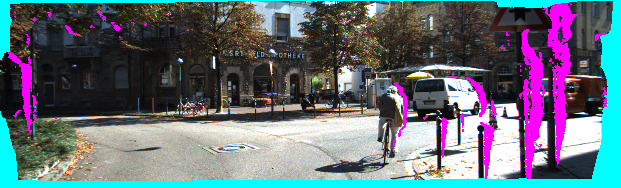
Figure 2. Illustration of the warping process with occlusion handling. The top images visualizes the geometry (virtual disparity) at time $t_{2}$ after warping towards the reference frame at time $t_{1}$. The bottom image shows the two types of obstruction, geometric occlusion (magenta) and out-of-view motion (cyan), which can be considered as occlusion by the camera frustum.

An illustration of gaps in the warped disparity map due to the two types of occlusions.

3.2. Warping and Occlusion Estimation

The auxiliary estimators provide the basis for our approach. However, warping is the actual core and biggest challenge for the combination method. It is needed to correlate the 3D information of different pixels to find the shift over time. In accordance with previous work (Schuster et al., 2018a), we define the warping operation to map the current and future depth values as follows:

(2) $$d^{w}_{2}(\mathbf{p})=d_{2}\left(\mathbf{p}+\mathbf{u}(\mathbf{p})\right)$$

During warping, we ignore target pixels outside of the image domain and use bilinear interpolation to account for sub-pixel displacements in the estimated optical flow. These out-of-bound regions lead to a non-dense warped disparity. Additionally, some points move in front or behind others so that not all points visible at $t_{1}$ are also visible at $t_{2}$. These occlusions need to be filtered, because they produce ghosting effects, i.e. duplicated objects, after warping. Since we have an estimate of depth, we can reason about which of these points occlude the others, masking all but the closest point for all source pixels with the same target position. This is formalized in Equation 3 by

(3) $$occ(\mathbf{p})=\left[d_{1}(\mathbf{p})<d_{1}(\mathbf{p^{\prime}})\forall\mathbf{p^{\prime}}\in\Omega\mid\mathbf{p^{\prime}}+\mathbf{u}(\mathbf{p^{\prime}})\approx\mathbf{p}+\mathbf{u}(\mathbf{p})\right]$$

to obtain a binary occlusion mask $occ$ for each pixel in the image domain $\Omega$, where $\left[\bullet\right]$ denotes the Iverson bracket and sub-pixel optical flow is handled by rounding.

After initial occlusion mask estimation, we correct discretization and rounding errors by applying two iterations of morphological closing and opening. An exemplary result of a warped disparity map and occlusion mask is given in Figure 2.

By combining the initially estimated optical flow $\mathbf{u}$, the geometric information of $d_{1}$ at time $t_{1}$, and the warped disparity $d_{2}^{w}$, a non-dense scene flow can be obtained. This intermediate result is analyzed in Section 4.1.

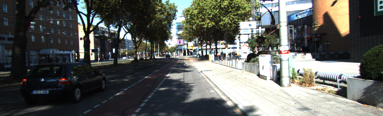
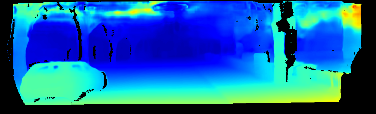
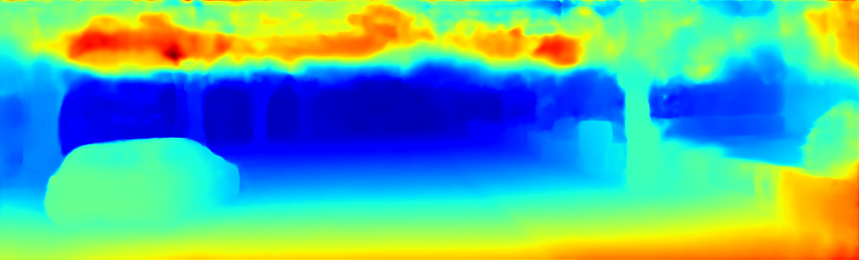
Figure 3. Visualization of a depth (virtual disparity) estimate from our validation split before and after interpolation with SSGP (Schuster et al., 2020).

The geometry of the scene is visualized before and after interpolation along with a reference image.

Table 1. Evaluation of different components and steps of our approach on the validation split of the KITTI scene flow training data. End-point-error (EPE, [px]) and KITTI outlier error (KOE, [%]) are given. Numbers in parentheses indicate that the respective model was (partially) trained on the validation data.

Method	D1		D2		OF		SF		Density
	EPE	KOE	EPE	KOE	EPE	KOE	$\Sigma$EPE	KOE
BTS (Lee et al., 2019) (original)	3.60	24.51	–	–	–	–	–	–	100 %
BTS (re-trained)	3.19	23.86	–	–	–	–	–	–	100 %
HD3 (Yin et al., 2019)	–	–	–	–	(1.74)	(5.13)	–	–	100 %
VCN (Yang and Ramanan, 2019)	–	–	–	–	(1.41)	(5.00)	–	–	100 %
BTS + HD3	2.99	20.18	3.42	26.28	(0.95)	(2.39)	7.35	29.04	81.89 %
BTS + VCN	2.98	20.15	3.36	25.44	(0.76)	(2.70)	7.10	28.07	81.70 %
BTS + HD3 + SSGP (Schuster et al., 2020) (D2)	3.19	23.86	3.21	24.01	(1.74)	(5.13)	8.14	35.08	100 %
BTS + VCN + SSGP (D2)	3.19	23.86	3.24	24.46	(1.41)	(5.00)	7.84	35.22	100 %
BTS + HD3 + SSGP (D1+D2)	2.76	20.30	3.21	24.01	(1.74)	(5.13)	7.70	29.50	100 %
BTS + VCN + SSGP (D1+D2)	2.76	20.30	3.24	24.46	(1.41)	(5.00)	7.41	29.34	100 %
BTS + SSGP (D1) + OE (Yang and Ramanan, 2020)	2.76	20.30	(3.36)	(23.63)	(2.02)	(7.01 )	8.14	26.53	100 %
BTS + OE	3.19	23.86	(3.90)	(27.87)	(2.02)	(7.01 )	9.10	30.60	100 %
MonoDepth2 (Godard et al., 2019) + OE	2.95	25.37	(3.54)	(28.47)	(2.02)	(7.01)	8.50	30.90	100 %

3.3. Interpolation and Refinement

To recover full density, we have to fill in the gaps of the warped disparity $d_{2}^{w}$. Our method of choice is SSGP (Schuster et al., 2020). SSGP is a recently presented network architecture for image-guided interpolation of different sparse or non-dense information. It was shown to work for optical flow, scene flow, or depth maps. We use it to interpolate the gaps in our warped virtual disparity map and name the interpolated output $d_{2}^{i}$. Because of the inverse target domain (disparity instead of depth), we retrain an implementation of SSGP on the KITTI depth data in the disparity space. This is achieved by conversion of all predicted values and ground truth depth labels with Equation 1 during loss computation. An example for warped, sparse geometry and the interpolated result is given in Figure 3. Note how in this example even the fully occluded bush on the right side is reconstructed reliably by the image guidance of SSGP.

In our experiments in Section 4.1, we show that the interpolation is able to reconstruct full density (with respect to the image resolution) and additionally to improve the predicted geometric information. We account this mostly to an correction of the absolute scale of depth (virtual disparity). This is similar to the two-stage depth estimation in Mono-SF (Brickwedde et al., 2019) where a dedicated network for re-calibration refines the initial depth estimates.

However, based on the observation that SSGP improves the results beyond interpolation, we suggest that this step might also improve already dense input, i.e. the (virtual) disparity estimate at time $t_{1}$. For this reason, our full model processes the dense estimate $d_{1}$ with SSGP before combining it into dense scene flow (cf. Figure 1). We term the refined disparity map $d_{1}^{r}$.

Lastly, all separate results ($\mathbf{u},d_{1}^{r},d_{2}^{i}$) are combined to form dense scene flow (in image space).

Table 2. Evaluation results from the KITTI benchmark for all submitted monocular scene flow approaches. We distinguish between supervised and unsupervised methods. Best (lowest) numbers in bold.

Method	D1 [%]			D2 [%]			OF [%]			SF [%]			Run time
	bg	fg	all	bg	fg	all	bg	fg	all	bg	fg	all
Mono-SF (Brickwedde et al., 2019)	14.21	26.94	16.32	16.89	33.07	19.59	11.40	19.64	12.77	19.79	39.57	23.08	41 s
MonoComb (ours)	17.89	21.16	18.44	22.34	25.85	22.93	5.84	8.67	6.31	27.06	33.55	28.14	0.58 s
MonoExpansion (Yang and Ramanan, 2020)	24.85	27.90	25.36	27.69	31.59	28.34	5.83	8.66	6.30	29.82	36.67	30.96	0.25 s
Self-Mono-SF-ft (Hur and Roth, 2020)	20.72	29.41	22.16	23.83	32.29	25.24	15.51	17.96	15.91	31.51	45.77	33.88	0.09 s
Self-Mono-SF (Hur and Roth, 2020)	31.22	48.04	34.02	34.89	43.59	36.34	23.26	24.93	23.54	46.68	63.82	49.54	0.09 s

4. Experiments and Results

In our experiments, the monocular combination approach is evaluated step-by-step – starting from the initial estimates until dense scene flow – and then compared to state-of-the-art on the KITTI scene flow benchmark (Geiger et al., 2012; Menze and Geiger, 2015). This data set provides realistic imagery for diverse traffic scenarios – including highway, suburban streets, and cities – as well as labels for full 3D scene flow. 200 sequences are labeled for training and another 200 sequences are provided as input for online evaluation with ground truth labels withhold. The models for monocular depth estimation are trained with the KITTI depth data set, which is much larger. These two data sets are related by an intersection of 142 sequences of the labeled training sets. Therefore, we define our validation split for scene flow as the remaining 58 sequences. The full list of these sequences is available in the official development kit of the KITTI scene flow data set.

For the evaluation, we consider the default metrics for scene flow as defined by KITTI. These are the average end-point-errors (EPE) in image space for the separate results, i.e. disparities at time $t_{1}$ (D1) and $t_{2}$ (D2) as well as optical flow (OF) and the average KITTI outlier rates (KOE), where an estimated value is defined as outlier if its EPE exceeds 3 px or 5 % of the magnitude of the ground truth value. Scene flow outliers are defined as union of the outliers of separate results, i.e. if either disparity values at $t_{1}$ or $t_{2}$, or optical flow is an outlier.

4.1. Ablation Study

In our ablation study, we evaluate separate parts and intermediate results of our approach individually. The results are presented in Table 1. In detail, we test the re-trained BTS (Lee et al., 2019) with disparity transformation on the scene flow validation set and notice a small improvement over the officially provided pre-trained weights. Further, the two considered estimators for optical flow, HD3 (Yin et al., 2019) and VCN (Yang and Ramanan, 2019), are evaluated. It is important to note, that we have not re-trained these networks and thus our validation split was entirely used during training of both, HD3 and VCN. This is indicated by parentheses in Table 1. That said, the generalization of the models to the unseen test set is not too bad as is shown by the results on the KITTI benchmark (cf. Table 2).

The important next step of our pipeline is the warping. The warped (virtual) disparities are also evaluated together with the sparse scene flow that is created by warping. We notice similar performance for both optical flow estimators, reaching densities of 81.9 and 81.7 %. It is further evident that the warping introduces some artifacts which reduce the accuracy compared to the disparity maps that are directly estimated in the respective reference frame. At the same time, the masking of occlusions and out-of-bounds motions also removes some outliers in the disparity at time $t_{1}$ and the optical flow. This reveals that HD3 has more difficulties to handle occlusion compared to VCN. Overall, as seen in previous work (Schuster et al., 2018a), the sparse scene flow obtained by warping is comparatively accurate, yet being non-dense.

To recover full density, $d^{w}_{2}$ is interpolated with SSGP. Interestingly, the interpolation does not only fill in the gaps, but further improves the dense result over the sparse one. For that reason, we finally apply dense refinement to $d_{1}$ using SSGP. This results in a significant reduction of errors for D1 and an even bigger improvement for the overall scene flow estimates. At the same time, the qualitative impressions in Figures 3 and 6(b) reveal that the interpolation and the dense refinement with SSGP introduce artifacts in the sky regions (upper third of the image) where no supervision signal is available in the data set.

Lastly, numbers for the competing method OE (Yang and Ramanan, 2020) are presented. This method uses every fifth frame (starting with sequence 0) for validation and the rest for training. As a consequence, part of our validation set has been used to train OE. The reference depth estimate for OpticalExpansion was computed with MonoDepth2 (Godard et al., 2019). We also report numbers when OE is used in conjunction with BTS and our refined disparity estimate $d_{1}^{r}$. We make this comparison to validate that our approach performs not just better because of the better depth estimator (BTS over MonoDepth2), but because of the way corresponding depth values over time are correlated. This is validated by the relatively little improvement of scene flow outliers (SF KOE) compared to the outliers of D1 in the last two rows of Table 1. The third last row validates that our contribution of dense refinement is also beneficial for other approaches.

4.2. Comparison to State-of-the-Art

In this experiment we compare our dense monocular scene flow approach to state-of-the-art in this field. This is done by submitting to the online KITTI scene flow benchmark. For that, SSGP for interpolation and dense refinement is re-trained on all 200 sequences of the KITTI training split. This turned out especially useful since our validation split is comparatively large ($>25\%$). Results for all published monocular approaches and our proposed method is shown in Table 2. The results of the ablation study (Table 1) are transferred within reasonable deviation and some further improvements due to the additional training data.

Our monocular combination approach (MonoComb) pushes state-of-art in various ways. We achieve the second best result overall and the best result among all methods with sub-second run time. Further, we achieve the lowest error rate for the important foreground regions (fg) of dynamic objects with a margin of more than 3 percentage points.

A qualitative comparison is provided in Figure 6(b) where the result of the first test frame for all monocular methods is visualized along with the corresponding error maps. This particular sample reveals the major issues of each approach. For Mono-SF (Brickwedde et al., 2019) the biggest challenge is the correct estimation of dynamic objects. This is also reflected by the quantitative results in Table 2. The monocular version of OpticalExpansion (Yang and Ramanan, 2020) (MonoExpansion), is depending a lot on the estimate of the initial depth/disparity. Further, since the relative change in depth is tightly coupled and estimated together with optical flow, the estimated second disparity suffers from the same limitations as optical flow, i.e. occlusions, visual perturbation by large geometric deformations over time, etc. The (fine-tuned) self-supervised approach (Hur and Roth, 2020) is mainly restricted by the lower level of details due to the reduced output resolution. Our proposed approach predicts scene flow at full resolution, handles occlusion explicitly and solves this issue by interpolation, and provides top performance for dynamic objects. However, the error maps in Figure 6(b) indicate that the absolute scale is not recovered sufficiently well. Further, the major limitation of our method is the inconsistency of the prediction due to the separation. This results in bad alignment of correct and erroneous regions across the separate tasks, and ultimately in a high outlier rate in the scene flow metric. In fact in Table 2, our approach has a much larger margin between the highest outlier rate of D1, D2, or OF and SF, compared to e.g. OpticalExpansion (Yang and Ramanan, 2020).

(a) Reference Image

Estimate

Error Map

D1

D1

D2

D2

OF

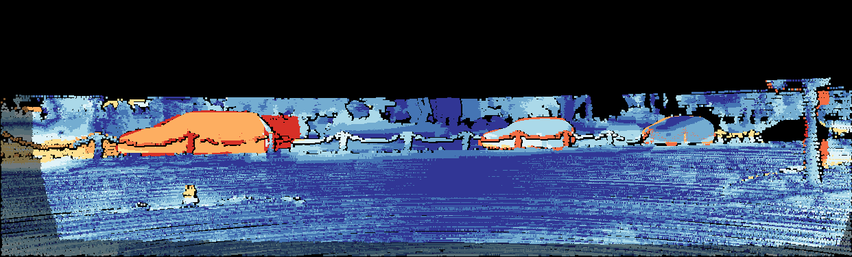
OF

EPE:

(b) Result of Mono-SF (Brickwedde et al., 2019)

Estimate

Error Map

D1

D1

D2

D2

OF

OF

EPE:

(c) Result of MonoExpansion (Yang and Ramanan, 2020)

Figure 4. Continued on the next page.

For all compared monocular scene flow approaches, a visualization of the results along with the corresponding error maps.

Estimate

Error Map

D1

D1

D2

D2

OF

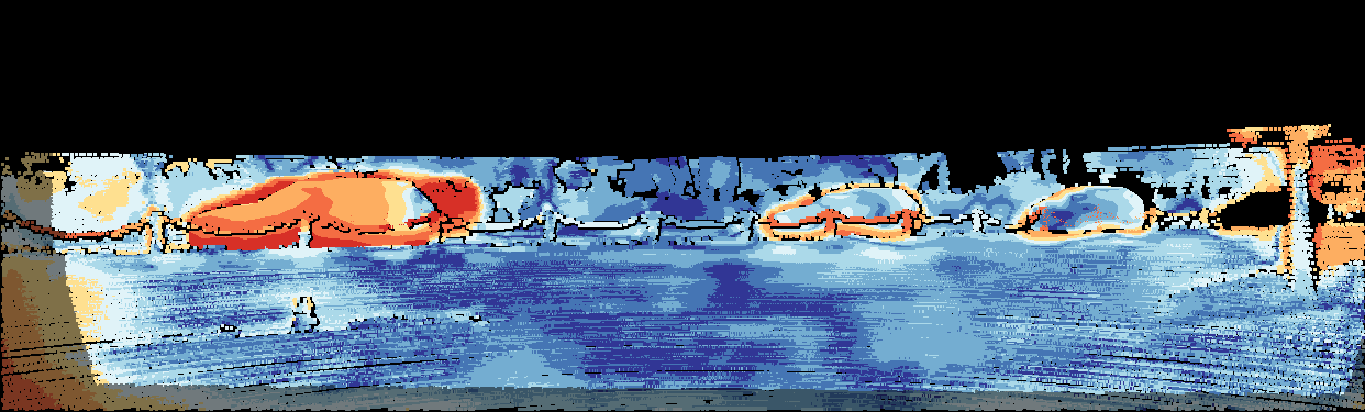
OF

EPE:

(a) Result of Self-Mono-SF (fine-tuned) (Hur and Roth, 2020)

Estimate

Error Map

D1

D1

D2

D2

OF

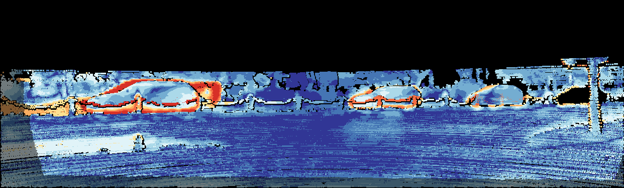
OF

EPE:

(b) Result of our monocular combination approach MonoComb.

Figure 6. Visualization and error maps from the KITTI online benchmark for the first test frame. We compare Mono-SF (Brickwedde et al., 2019) (4(b)), MonoExpansion (Yang and Ramanan, 2020) (4(c)), Self-Mono-SF (Hur and Roth, 2020) (6(a)), and our proposed approach (6(b)).

For all compared monocular scene flow approaches, a visualization of the results along with the corresponding error maps.

4.3. Run Time

One advantage of the combination approach is the modularity. As part of that, the overall run time is defined by the sum of the auxiliary run times as given by Table 3. In our case this leads to an approximate average run time per frame of 0.58 seconds. This sums up over two runs of the single image depth estimator, one forward pass of the optical flow estimator, and two runs of SSGP for refinement and interpolation. The time for warping and combination of the separate results is neglectable small.

Table 3. Breakdown of the run time.

Module	Calls	Run time
HD3 (Yin et al., 2019) / VCN (Yang and Ramanan, 2019)	1	0.1 / 0.18 s
BTS (Lee et al., 2019)	2	0.06 s
SSGP (Schuster et al., 2020)	2	0.14 s
Total	–	0.5 / 0.58 s

5. Conclusion

The sparse-to-dense re-combination approach for scene flow estimation is successfully transferred to the monocular camera setup. This is achieved by latest success in single image depth estimation and robust sparse-to-dense interpolation. Together with state-of-the-art auxiliary estimators, the proposed concept achieves more than competitive results at reasonable speed. The modularity of the approach allows to quickly replace parts of the pipeline to tune the overall performance towards a certain goal, i.e. real time performance.

In this relatively new discipline of monocular scene flow estimation, the monocular combination approach can be seen as a strong baseline for future developments.

The biggest limitation of our method is the inconsistency of the separate results. To overcome this in the future, we propose to perform interpolation and dense refinement jointly, which might also introduce mutual advantages for both tasks. Additionally, the monocular camera setup for scene flow estimation does not restrict the depth estimation to use a single image. It should be investigated whether the joint estimation of depth over time (e.g. two-view depth estimation) can improve the results further.

- (1)
- Battrawy et al. (2019) Ramy Battrawy, René Schuster, Oliver Wasenmüller, Qing Rao, and Didier Stricker. 2019. LiDAR-Flow: Dense Scene Flow Estimation from Sparse LiDAR and Stereo Images. In International Conference on Intelligent Robots and Systems (IROS).
- Behl et al. (2019) Aseem Behl, Despoina Paschalidou, Simon Donne, and Andreas Geiger. 2019. PointFlowNet: Learning Representations for Rigid Motion Estimation from Point Clouds. In Conference on Computer Vision and Pattern Recognition (CVPR).
- Brickwedde et al. (2019) Fabian Brickwedde, Steffen Abraham, and Rudolf Mester. 2019. Mono-SF: Multi-view geometry meets single-view depth for monocular scene flow estimation of dynamic traffic scenes. In International Conference on Computer Vision (ICCV).
- Fu et al. (2018) Huan Fu, Mingming Gong, Chaohui Wang, Kayhan Batmanghelich, and Dacheng Tao. 2018. Deep ordinal regression network for monocular depth estimation. In Conference on Computer Vision and Pattern Recognition (CVPR).
- Geiger et al. (2012) Andreas Geiger, Philip Lenz, and Raquel Urtasun. 2012. Are we ready for autonomous driving? The KITTI vision benchmark suite. In Conference on Computer Vision and Pattern Recognition (CVPR).
- Godard et al. (2017) Clément Godard, Oisin Mac Aodha, and Gabriel J Brostow. 2017. Unsupervised monocular depth estimation with left-right consistency. In Conference on Computer Vision and Pattern Recognition (CVPR).
- Godard et al. (2019) Clément Godard, Oisin Mac Aodha, Michael Firman, and Gabriel J Brostow. 2019. Digging into self-supervised monocular depth estimation. In International Conference on Computer Vision (ICCV).
- Herbst et al. (2013) Evan Herbst, Xiaofeng Ren, and Dieter Fox. 2013. RGB-D Flow: Dense 3-D motion estimation using color and depth. In International Conference on Robotics and Automation (ICRA).
- Hornacek et al. (2014) Michael Hornacek, Andrew Fitzgibbon, and Carsten Rother. 2014. SphereFlow: 6 DoF scene flow from RGB-D pairs. In Conference on Computer Vision and Pattern Recognition (CVPR).
- Huguet and Devernay (2007) Frédéric Huguet and Frédéric Devernay. 2007. A variational method for scene flow estimation from stereo sequences. In International Conference on Computer Vision (ICCV).
- Hur and Roth (2020) Junhwa Hur and Stefan Roth. 2020. Self-Supervised Monocular Scene Flow Estimation. In Conference on Computer Vision and Pattern Recognition (CVPR).
- Lee et al. (2019) Jin Han Lee, Myung-Kyu Han, Dong Wook Ko, and Il Hong Suh. 2019. From big to small: Multi-scale local planar guidance for monocular depth estimation. arXiv preprint arXiv:1907.10326 (2019).
- Liu et al. (2019) Xingyu Liu, Charles R Qi, and Leonidas J Guibas. 2019. FlowNet3D: Learning scene flow in 3d point clouds. In Conference on Computer Vision and Pattern Recognition (CVPR).
- Menze and Geiger (2015) Moritz Menze and Andreas Geiger. 2015. Object scene flow for autonomous vehicles. In Conference on Computer Vision and Pattern Recognition (CVPR).
- Ochs et al. (2019) Matthias Ochs, Adrian Kretz, and Rudolf Mester. 2019. SDNet: Semantically guided depth estimation network. In German Conference on Pattern Recognition (GCPR).
- Rishav et al. (2020) Rishav, Ramy Battrawy, René Schuster, Oliver Wasenmüller, and Didier Stricker. 2020. DeepLiDARFlow: A Deep Learning Architecture For Scene Flow Estimation Using Monocular Camera and Sparse LiDAR. In International Conference on Intelligent Robots and Systems (IROS).
- Schuster et al. (2018a) René Schuster, Christian Bailer, Oliver Wasenmüller, and Didier Stricker. 2018a. Combining Stereo Disparity and Optical Flow for Basic Scene Flow. In Commercial Vehicle Technology Symposium (CVT).
- Schuster et al. (2018c) René Schuster, Oliver Wasenmuller, Georg Kuschk, Christian Bailer, and Didier Stricker. 2018c. SceneFlowFields: Dense Interpolation of Sparse Scene Flow Correspondences. In Winter Conference on Applications of Computer Vision (WACV).
- Schuster et al. (2018b) René Schuster, Oliver Wasenmüller, and Didier Stricker. 2018b. Dense Scene Flow from Stereo Disparity and Optical Flow. In Computer Science in Cars Symposium (CSCS).
- Schuster et al. (2020) René Schuster, Oliver Wasenmüller, Christian Unger, and Didier Stricker. 2020. SSGP: Sparse Spatial Guided Propagation for Robust and Generic Interpolation. In Winter Conference on Applications of Computer Vision (WACV).
- Sun et al. (2018) Deqing Sun, Xiaodong Yang, Ming-Yu Liu, and Jan Kautz. 2018. PWC-Net: CNNs for optical flow using pyramid, warping, and cost volume. In Conference on Computer Vision and Pattern Rrecognition (CVPR).
- Uhrig et al. (2017) Jonas Uhrig, Nick Schneider, Lukas Schneider, Uwe Franke, Thomas Brox, and Andreas Geiger. 2017. Sparsity invariant cnns. In International Conference on 3D Vision (3DV).
- Vedula et al. (2005) Sundar Vedula, Peter Rander, Robert Collins, and Takeo Kanade. 2005. Three-dimensional scene flow. Transactions on Pattern Analysis and Machine Intelligence (T-PAMI) (2005).
- Vogel et al. (2013) Christoph Vogel, Konrad Schindler, and Stefan Roth. 2013. Piecewise rigid scene flow. In International Conference on Computer Vision (ICCV).
- Wang et al. (2020) Zirui Wang, Shuda Li, Henry Howard-Jenkins, Victor Prisacariu, and Min Chen. 2020. FlowNet3D++: Geometric losses for deep scene flow estimation. In Winter Conference on Applications of Computer Vision (WACV).
- Wedel et al. (2008) Andreas Wedel, Clemens Rabe, Tobi Vaudrey, Thomas Brox, Uwe Franke, and Daniel Cremers. 2008. Efficient dense scene flow from sparse or dense stereo data. In European Conference on Computer Vision (ECCV).
- Yang and Ramanan (2019) Gengshan Yang and Deva Ramanan. 2019. Volumetric correspondence networks for optical flow. In Advances in Neural Information Processing Systems (NeurIPS).
- Yang and Ramanan (2020) Gengshan Yang and Deva Ramanan. 2020. Upgrading Optical Flow to 3D Scene Flow through Optical Expansion. In Conference on Computer Vision and Pattern Recognition (CVPR).
- Yin et al. (2019) Zhichao Yin, Trevor Darrell, and Fisher Yu. 2019. Hierarchical discrete distribution decomposition for match density estimation. In Conference on Computer Vision and Pattern Recognition (CVPR).