\ul
Self-supervised Graph Learning for Recommendation
Abstract.
Representation learning on user-item graph for recommendation has evolved from using single ID or interaction history to exploiting higher-order neighbors. This leads to the success of graph convolution networks (GCNs) for recommendation such as PinSage and LightGCN. Despite effectiveness, we argue that they suffer from two limitations: (1) high-degree nodes exert larger impact on the representation learning, deteriorating the recommendations of low-degree (long-tail) items; and (2) representations are vulnerable to noisy interactions, as the neighborhood aggregation scheme further enlarges the impact of observed edges.
In this work, we explore self-supervised learning on user-item graph, so as to improve the accuracy and robustness of GCNs for recommendation. The idea is to supplement the classical supervised task of recommendation with an auxiliary self-supervised task, which reinforces node representation learning via self-discrimination. Specifically, we generate multiple views of a node, maximizing the agreement between different views of the same node compared to that of other nodes. We devise three operators to generate the views — node dropout, edge dropout, and random walk — that change the graph structure in different manners. We term this new learning paradigm as Self-supervised Graph Learning (SGL), implementing it on the state-of-the-art model LightGCN. Through theoretical analyses, we find that SGL has the ability of automatically mining hard negatives. Empirical studies on three benchmark datasets demonstrate the effectiveness of SGL, which improves the recommendation accuracy, especially on long-tail items, and the robustness against interaction noises. Our implementations are available at https://github.com/wujcan/SGL.
1. Introduction
Learning high-quality user and item representations from interaction data is the theme of collaborative recommendation. Earlier work like matrix factorization (MF) (Rendle et al., 2009) projects single ID of each user (or item) into an embedding vector. Some follow-on studies (Koren, 2008; He et al., 2018) enrich the single ID with interaction history for learning better representations. More recently, representation learning has evolved to exploiting higher-order connectivity in user-item graph. The technique is inspired from the graph convolution networks (GCNs), which provide an end-to-end way to integrate multi-hop neighbors into node representation learning and achieve state-of-the-art performance for recommendation (Wang et al., 2019b; He et al., 2020a; van den Berg et al., 2017; Ying et al., 2018).
Despite effectiveness, current GCN-based recommender models suffer from some limitations:
-
•
Sparse Supervision Signal. Most models approach the recommendation task under a supervised learning paradigm (Rendle et al., 2009; He et al., 2017, 2020a), where the supervision signal comes from the observed user-item interactions. However, the observed interactions are extremely sparse (He and McAuley, 2016; Bayer et al., 2017) compared to the whole interaction space, making it insufficient to learn quality representations.
-
•
Skewed Data Distribution. Observed interactions usually exhibit a power-law distribution (Clauset et al., 2009; Milojevic, 2010), where the long tail consists of low-degree items that lack supervision signal. In contrast, high-degree items appear more frequently in neighborhood aggregation and supervised loss, thus exert larger impact on representation learning. Hence, the GCNs are easily biased towards high-degree items (Tang et al., 2020; Chen et al., 2020a), sacrificing the performance of low-degree (long-tail) items.
-
•
Noises in Interactions. Most feedback that a user provides is implicit (e.g., clicks, views), instead of explicit (e.g., ratings, likes/dislikes). As such, observed interactions usually contain noises, e.g., a user is misled to click an item and finds it uninteresting after consuming it (Wang et al., 2021). The neighborhood aggregation scheme in GCNs enlarges the impact of interactions on representation learning, making the learning more vulnerable to interaction noises.
In this work, we focus on exploring self-supervised learning (SSL) in recommendation, to solve the foregoing limitations. Though being prevalent in computer vision (CV) (Gidaris et al., 2018; van den Oord et al., 2018) and natural language processing (NLP) (Devlin et al., 2019; Lan et al., 2020), SSL is relatively less explored in recommendation. The idea is to set an auxiliary task that distills additional signal from the input data itself, especially through exploiting the unlabeled data space. For example, BERT (Devlin et al., 2019) randomly masks some tokens in a sentence, setting the prediction of the masked tokens as the auxiliary task that can capture the dependencies among tokens; RotNet (Gidaris et al., 2018) randomly rotates labeled images, training the model on the rotated images to get improved representations for the mask task of object recognition or image classification. Compared with supervised learning, SSL allows us to exploit the unlabeled data space via making changes on the input data, achieving remarkable improvements in downstream tasks (Chen et al., 2020b).
Here we wish to bring the SSL’s superiority into recommendation representation learning, which differs from CV/NLP tasks since the data are discrete and inter-connected. To address the aforementioned limitations of GCN-based recommendation models, we construct the auxiliary task as discriminating the representation of a node itself. Specifically, it consists of two key components: (1) data augmentation, which generates multiple views for each node, and (2) contrastive learning, which maximizes the agreement between different views of the same node, compared to that of other nodes. For GCNs on user-item graph, the graph structure serves as the input data that plays an essential role for representation learning. From this view, it is natural to construct the ”unlabeled” data space by changing the graph adjacency matrix, and we develop three operators to this end: node dropout, edge dropout, and random walk, where each operator works with a different rationality. Thereafter, we perform contrastive learning based on the GCNs on the changed structure. As a result, SGL augments the node representation learning by exploring the internal relationship among nodes.
Conceptually, our SGL supplements existing GCN-based recommendation models in: (1) node self-discrimination offers auxiliary supervision signal, which is complementary to the classical supervisions from observed interactions only; (2) the augmentation operators, especially edge dropout, helps to mitigate the degree biases by intentionally reducing the influence of high-degree nodes; (3) the multiple views for nodes w.r.t. different local structures and neighborhoods enhance the model robustness against interaction noises. Last but not least, we offer theoretical analyses for the contrastive learning paradigm, finding that it has the side effect of mining hard negative examples, which not only boosts the performance but also accelerates the training process.
It is worthwhile mentioning that our SGL is model-agnostic and can be applied to any graph-based model that consists of user and/or item embedding. Here we implement it on the simple but effective model, LightGCN (He et al., 2020a). Experimental studies on three benchmark datasets demonstrate the effectiveness of SGL, which significantly improves the recommendation accuracy, especially on long-tail items, and enhance the robustness against interaction noises. We summarize the contributions of this work as follows:
-
•
We devise a new learning paradigm, SGL, which takes node self-discrimination as the self-supervised task to offer auxiliary signal for representation learning.
-
•
In addition to mitigating degree bias and increasing robustness to interaction noises, we prove in theory that SGL inherently encourages learning from hard negatives, controlled by the temperature hyper-parameter in the softmax loss function.
-
•
We conduct extensive experiments on three benchmark datasets to demonstrate the superiority of SGL.
2. Preliminaries
We first summarize the common paradigm of GCN-based collaborative filtering models. Let and be the set of users and items respectively. Let be the observed interactions, where indicates that user has adopted item before. Most existing models (Wang et al., 2019b; He et al., 2020a; van den Berg et al., 2017) construct a bipartite graph , where the node set involves all users and items, and the edge set represents observed interactions.
Recap GCN. At the core is to apply the neighborhood aggregation scheme on , updating the representation of ego node by aggregating the representations of neighbor nodes:
| (1) |
where denotes the node representations at the -th layer, is that of previous layer, and is the ID embeddings (trainable parameters). denotes the function for neighborhood aggregation, which is more interpretable from the vector level:
| (2) |
To update the representation of ego node at the -th layer, it first aggregates the representations of its neighbors at the -th layer, then combines with its own representation . There are a number of designs for and (Hamilton et al., 2017; Gilmer et al., 2017; Velickovic et al., 2018; Xu et al., 2019). We can see that the representations of the -th layer encode the -order neighbors in the graph. After obtaining layers representations, there may be a readout function to generate the final representations for prediction:
| (3) |
Common designs include last-layer only (van den Berg et al., 2017; Ying et al., 2018), concatenation (Wang et al., 2019b), and weighted sum (He et al., 2020a).
Supervised Learning Loss. A prediction layer is built upon the final representations to predict how likely would adopt . A classical solution is the inner product, which supports fast retrieval:
| (4) |
To optimize model parameters, existing works usually frame the task as one of supervised learning, where the supervision signal comes from the observed interactions (also the edges of ). For example, encouraging the predicted value to be close to the ground truth value and selecting negative examples from missing data (He et al., 2017). Besides above point-wise learning, another common choice is the pairwise Bayesian Personalized Ranking (BPR) loss (Rendle et al., 2009), which enforces the prediction of an observed interaction to be scored higher than its unobserved counterparts:
| (5) |
where is the training data, and is the unobserved interactions. In this work, we choose it as the main supervised task.
3. Methodology
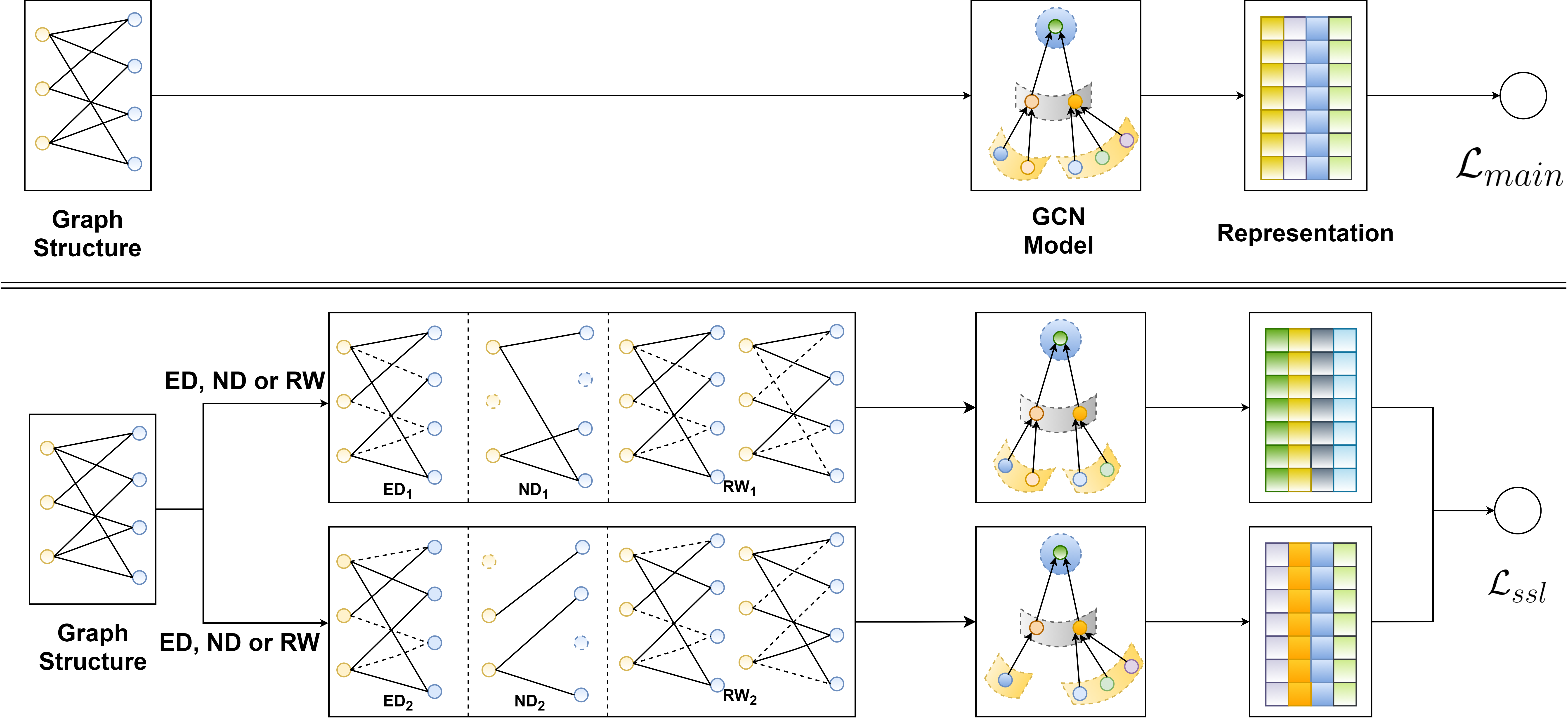
We present the proposed Self-supervised Graph Learning (SGL) paradigm, which supercharges the main supervised task with self-supervised learning. Figure 1 illustrates the working flow of SGL. Specifically, the self-supervised task (also termed as pretext task or auxiliary task) is to construct supervision signal from the correlation within the input data.
Specifically, we introduce how to perform data augmentation that generates multiple representation views, followed by the contrastive learning based on the generated representations to build the pretext task. SSL is combined with classical GCN in a multi-task learning manner. Thereafter, we conduct theoretical analyses on SSL from the gradient level, revealing the connection with hard negative mining. Lastly, we analyze the complexity of SGL.
3.1. Data Augmentation on Graph Structure
Directly grafting the data augmentation adopted in CV and NLP tasks (Wu et al., 2018; Chen et al., 2020b; He et al., 2020b; Devlin et al., 2019) is infeasible for graph-based recommendation, due to specific characteristics: (1) The features of users and items are discrete, like one-hot ID and other categorical variables. Hence, the augmentation operators on images, such as random crop, rotation, or blur, are not applicable. (2) More importantly, unlike CV and NLP tasks that treat each data instance as isolated, users and items in the interaction graph are inherently connected and dependent on each others. Thus, we need new augmentation operators tailored for graph-based recommendation.
The bipartite graph is built upon observed user-item interactions, thus containing the collaborative filtering signal. Specifically, the first-hop neighborhood directly profiles ego user and item nodes — i.e., historical items of a user (or interacted users of an item) can be viewed as the pre-existing features of user (or item). The second-hop neighboring nodes of a user (or an item) exhibit similar users w.r.t. behaviors (or similar items w.r.t. audiences). Furthermore, the higher-order paths from a user to an item reflect potential interests of the user on the item. Undoubtedly, mining the inherent patterns in graph structure is helpful to representation learning. We hence devise three operators on the graph structure, node dropout, edge dropout and random walk, to create different views of nodes. The operators can be uniformly expressed as follows:
| (6) |
where two stochastic selections and are independently applied on graph , and establish two correlated views of nodes and . We elaborate the augmentation operators as follows:
-
•
Node Dropout (ND). With the probability , each node is discarded from the graph, together with its connected edges. In particular, and can be modeled as:
(7) where are two masking vectors which are applied on the node set to generate two subgraphs. As such, this augmentation is expected to identify the influential nodes from differently augmented views, and make the representation learning less sensitive to structure changes.
-
•
Edge Dropout (ED). It drops out the edges in graph with a dropout ratio . Two independent processes are represented as:
(8) where are two masking vectors on the edge set . Only partial connections within the neighborhood contribute to the node representations. As such, coupling these two subgraphs together aims to capture the useful patterns of the local structures of a node, and further endows the representations more robustness against noisy interactions.
-
•
Random Walk (RW). The above two operators generate a subgraph shared across all the graph convolution layers. To explore higher capability, we consider assigning different layers with different subgraphs. This can be seen as constructing an individual subgraph for each node with random walk (Qiu et al., 2020) (see Figure 2 as an example). Assuming we choose edge dropout at each layer (with different ratio or random seeds), we can formulate RW by making the masking vector to be layer sensitive:
(9) where are two masking vectors on the edge set at layer .
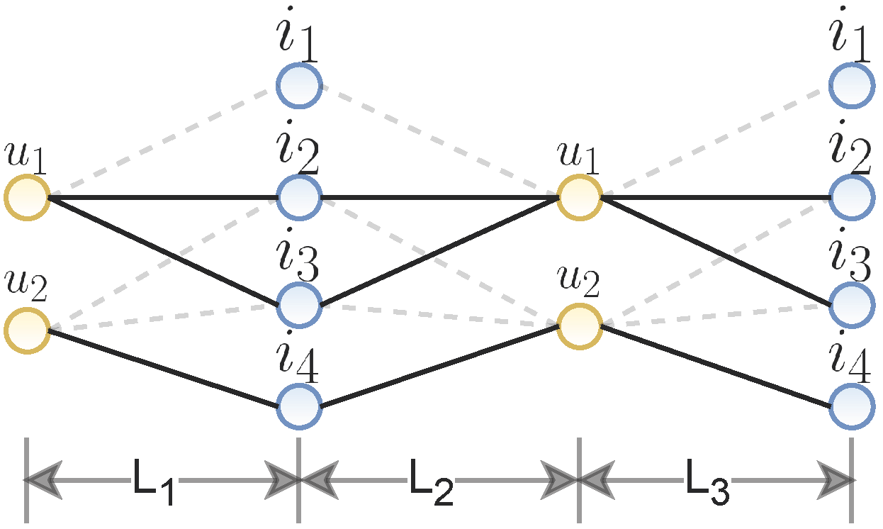
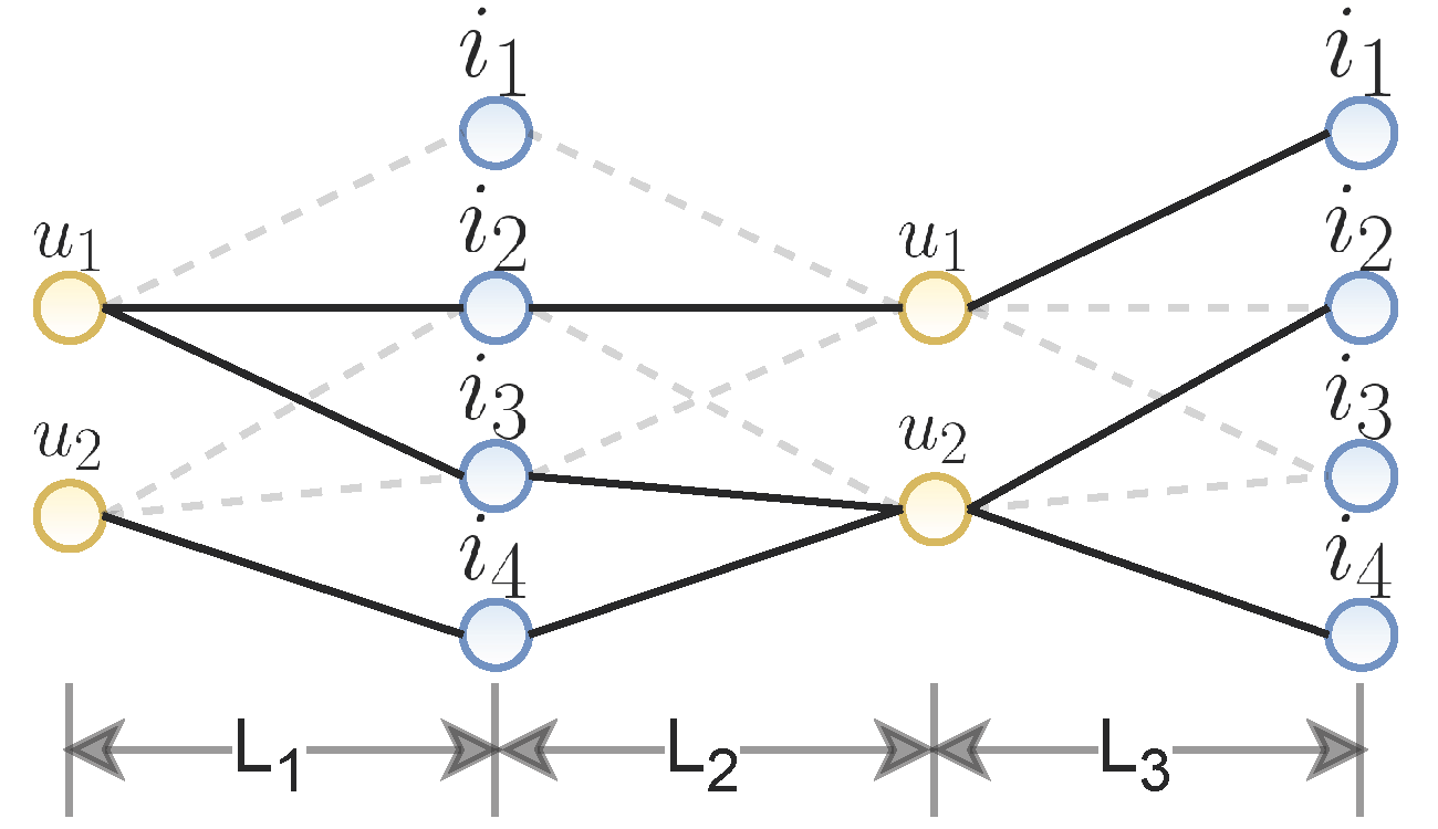
We apply these augmentations on graph structure per epoch for simplicity — that is, we generate two different views of each node at the beginning of a new training epoch (for RW, two different views are generated at each layer). Note that the dropout and masking ratios remain the same for two independent processes (i.e., and ). We leaving the tuning of different ratios in future work. It is also worthwhile mentioning that only dropout and masking operations are involved, and no any model parameters are added.
3.2. Contrastive Learning
Having established the augmented views of nodes, we treat the views of the same node as the positive pairs (i.e., ), and the views of any different nodes as the negative pairs (i.e., ). The auxiliary supervision of positive pairs encourages the consistency between different views of the same node for prediction, while the supervision of negative pairs enforces the divergence among different nodes. Formally, we follow SimCLR (Chen et al., 2020b) and adopt the contrastive loss, InfoNCE (Gutmann and Hyvärinen, 2010), to maximize the agreement of positive pairs and minimize that of negative pairs:
| (10) |
where measures the similarity between two vectors, which is set as cosine similarity function; is the hyper-parameter, known as the in softmax. Analogously, we obtain the contrastive loss of the item side . Combining these two losses, we get the objective function of self-supervised task as .
3.3. Multi-task Training
To improve recommendation with the SSL task, we leverage a multi-task training strategy to jointly optimize the classic recommendation task (cf. Equation (5)) and the self-supervised learning task (cf. Equation (10))
| (11) |
where is the set of model parameters in since introduces no additional parameters; and are hyperparameters to control the strengths of SSL and regularization, respectively. We also consider the alternative optimization — pre-training on and fine-tuning on . See more details in Section 4.4.2.
3.4. Theoretical Analyses of SGL
In this section, we offer in-depth analyses of SGL, aiming to answer the question: how does the recommender model benefit from the SSL task? Towards this end, we probe the self-supervised loss in Equation (10) and find one reason: it has the intrinsic ability to perform hard negative mining, which contributes large and meaningful gradients to the optimization and guides the node representation learning. In what follows, we present our analyses step by step.
Formally, for node , the gradient of the self-supervised loss w.r.t. the representation is as follows:
| (12) |
where is the individual term for a single node in Equation (10); is another node which serves as the negative view for node ; and separately represent the contribution of positive node and negative nodes to the gradients w.r.t. :
| (13) | |||
| (14) |
where ; and are the normalized representations of node from different views; similar notations to node . Afterwards, we focus on the contribution of negative node (cf. Equation (14)), the norm of which is proportional to the following term:
| (15) |
As and are both unit vectors, we can introduce another variable to simplify Equation (15) as follows:
| (16) |
where directly reflects the representation similarity between the positive node and the negative node . According to the similarity , we can roughly categorize the negative nodes into two groups: (1) Hard negative nodes, whose representations are similar to that of the positive node (i.e., ), thus making it difficult to distinguish from in the latent space; (2) Easy negative nodes, which are dissimilar to the positive node (i.e., ) and can be easily discriminated. To investigate the contributions of hard and easy negatives, we plot the curves of over the change of the node similarity in Figures 3(a) and 3(b), by setting and respectively. Clearly, under different conditions of , the contributions of negative nodes differ dramatically with each others. Specifically, as Figure 3(a) shows, given , the values of fall into the range of and slightly change in response to . This suggests that negative samples, no matter hard or easy, contribute similarly to the gradient. In contrast, as Figure 3(b) displays, when setting , the values of at hard negatives could reach , while the contribution of easy negatives is vanishing. This indicates that hard negative nodes offer much larger gradients to guide the optimization, thus making node representations more discriminative and accelerating the training process (Rendle and Freudenthaler, 2014).
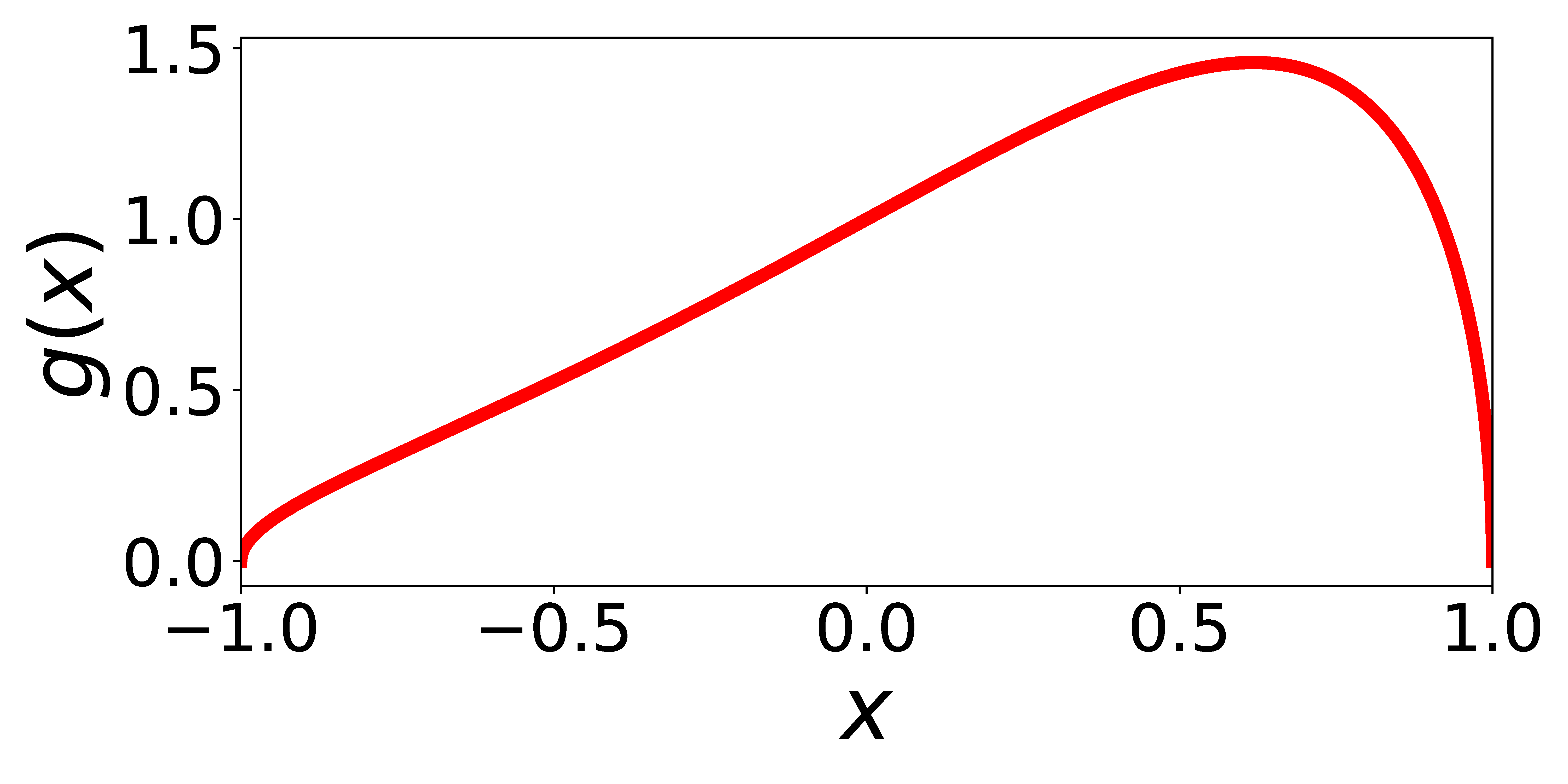
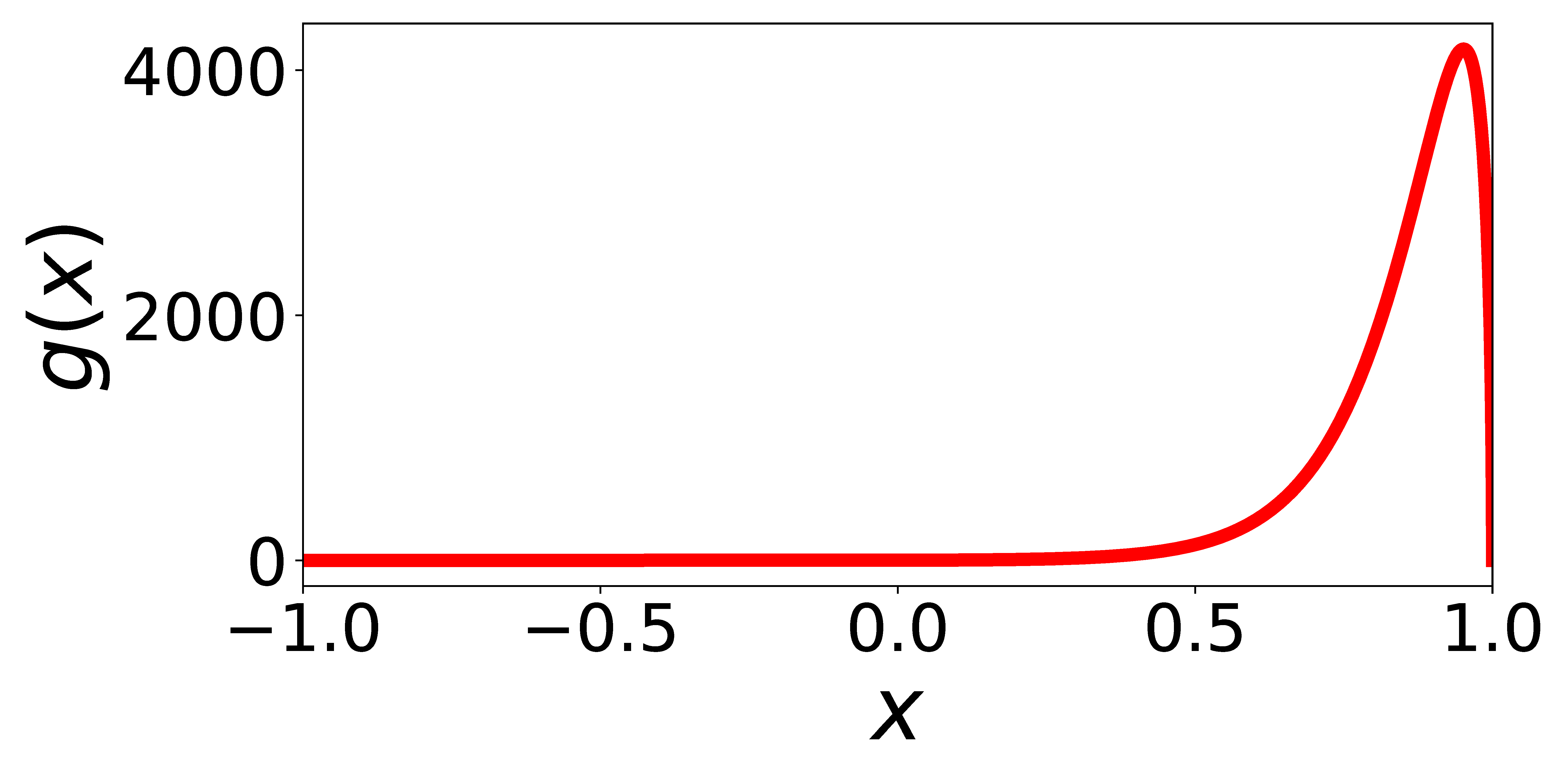
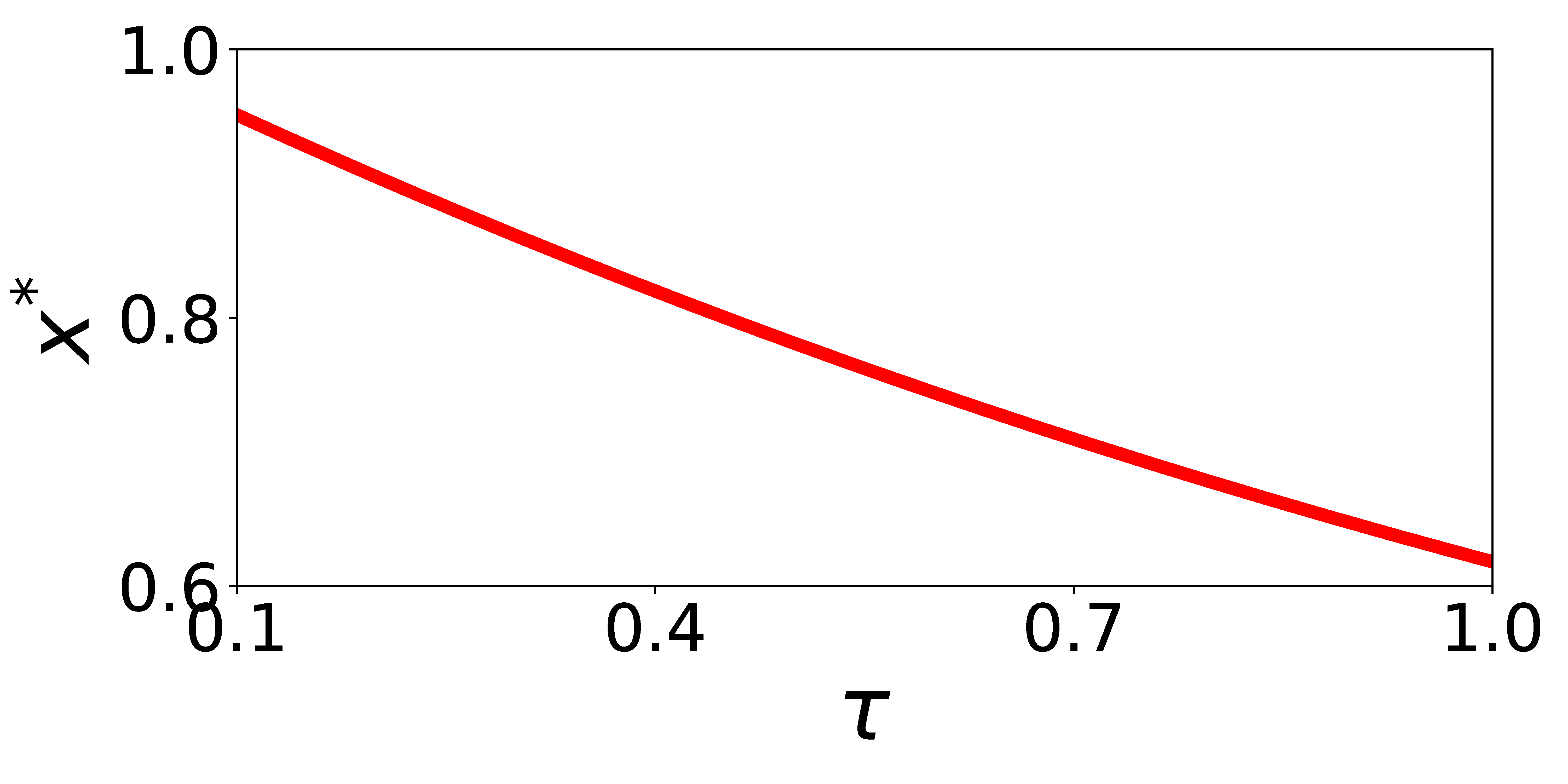
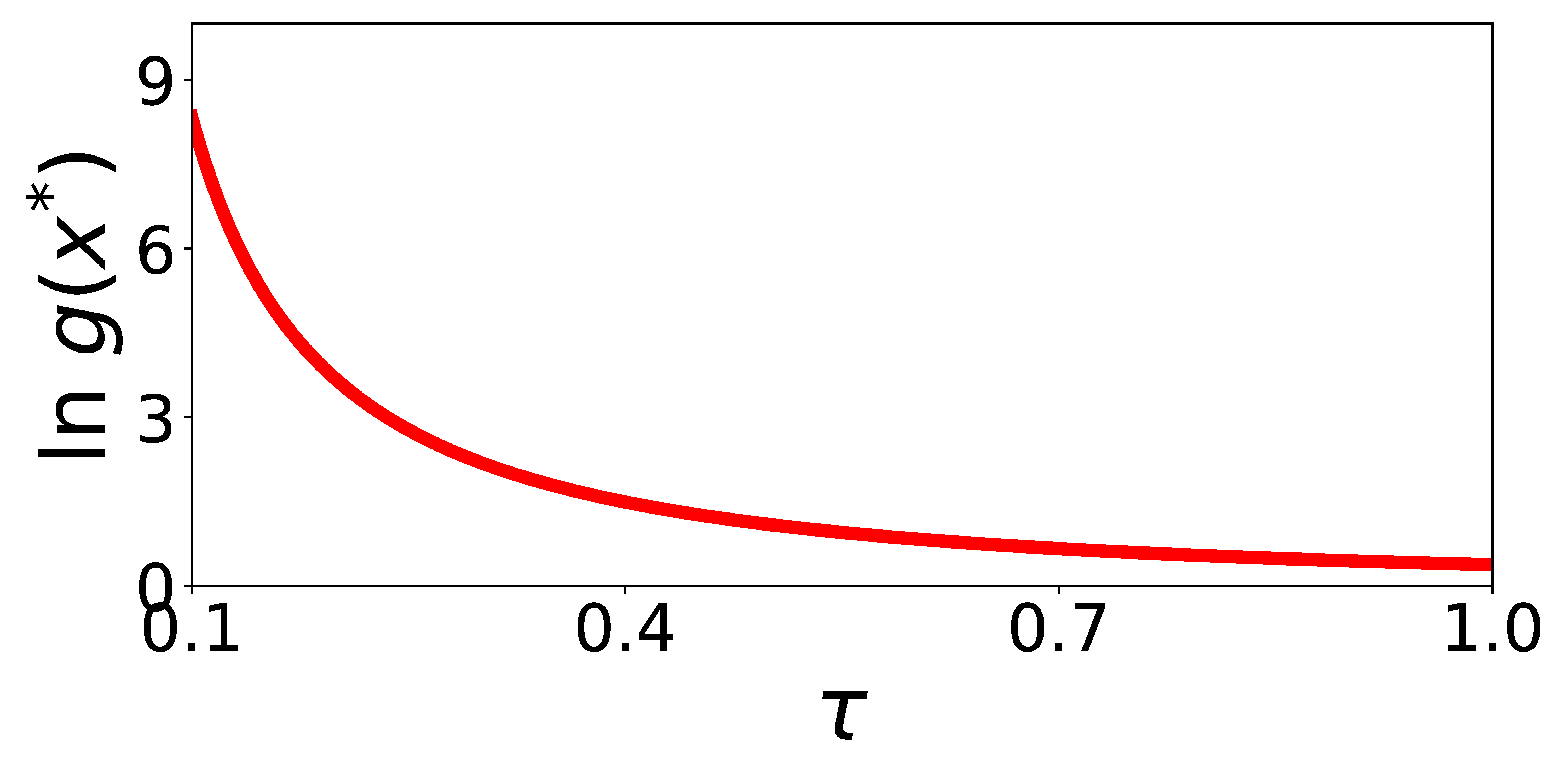
These findings inspire us to probe the influence of on the maximum value of . By approaching ’s derivative to zero, we can obtain with maximum value . To see how changes with , we represent its logarithm as:
| (17) |
We present the curves of and in Figures 3(c) and 3(d), respectively. With the decrease of , the most influential negative nodes become more similar to the positive node (i.e., approaches ), moreover, their contributions are amplified super-exponentially (i.e., is close to ). Hence, properly setting enables SGL to automatically perform hard negative mining.
It is worth mentioning that, our analyses are inspired by the prior study (Khosla et al., 2020), but there are major differences: (1) (Khosla et al., 2020) defines hard negatives as samples whose similarity are near-to-zero to the positive sample (i.e., ), and easy negatives as obviously dissimilar samples (i.e., ); (2) It leaves the region of untouched, which is however crucial in our case. Innovatively, we provide a more fine-grained view in the region of to highlight the critical role of , the temperature hyper-parameter in softmax, in mining hard negatives.
3.5. Complexity Analyses of SGL
In this subsection, we analyze the complexity of SGL with ED as the strategy and LightGCN as the recommendation model; other choices can be analyzed similarly. Since SGL introduces no trainable parameters, the space complexity remains the same as LightGCN (He et al., 2020a). The time complexity of model inference is also the same, since there is no change on the model structure. In the following part, we will analyze the time complexity of SGL training.
Suppose the number of nodes and edges in the user-item interaction graph are and respectively. Let denote the number of epochs, denote the size of each training batch, denote the embedding size, denote the number of GCN layers, denote the keep probability of SGL-ED. The complexity mainly comes from two parts:
-
•
Normalization of adjacency matrix. Since we generate two independent sub-graphs per epoch, given the fact that the number of non-zero elements in the adjacency matrices of full training graph and two sub-graph are and respectively, its total complexity is .
-
•
Evaluating self-supervised loss. We only consider the inner product in our analyses. As defined in Equation (10), we treat all other user nodes as negative samples when calculating InfoNCE loss of user side. Within a batch, the complexity of numerator and denominator are and , respectively, where is the number of users. And hence the total complexity of both user and item side per epoch is . Therefore, the time complexity of the whole training phase is . An alternative to reduce the time complexity is treating only the users (or the items) within the batch as negative samples (Chen et al., 2020b; Yao et al., 2020), resulting in total time complexity of .
We summarize the time complexity in training between LightGCN and SGL-ED in Table 1. The analytical complexity of LightGCN and SGL-ED is actually in the same magnitude, since the increase of LightGCN only scales the complexity of LightGCN. In practice, taking the Yelp2018 data as an example, the time complexity of SGL-ED (alternative) with of 0.8 is about 3.7x larger than LightGCN, which is totally acceptable considering the speedup of convergence speed we will show in Section 4.3.2. The testing platform is Nvidia Titan RTX graphics card equipped with Inter i7-9700K CPU (32GB Memory). The time cost of each epoch on Yelp2018 is 15.2s and 60.6s for LightGCN and SGL-ED (alternative) respectively, which is consistent with the complexity analyses.
| Component | LightGCN | SGL-ED | ||
|
||||
|
||||
|
||||
| Self-supervised Loss | - | |||
4. Experiments
| Dataset | #Users | #Items | #Interactions | Density |
|---|---|---|---|---|
| Yelp2018 | 31,668 | 38,048 | 1,561,406 | 0.00130 |
| Amazon-Book | 52,643 | 91,599 | 2,984,108 | 0.00062 |
| Alibaba-iFashion | 300,000 | 81,614 | 1,607,813 | 0.00007 |
To justify the superiority of SGL and reveal the reasons of its effectiveness, we conduct extensive experiments and answer the following research questions:
-
•
RQ1: How does SGL perform w.r.t. top- recommendation as compared with the state-of-the-art CF models?
-
•
RQ2: What are the benefits of performing self-supervised learning in collaborative filtering?
-
•
RQ3: How do different settings influence the effectiveness of the proposed SGL?
| Datase | Yelp2018 | Amazon-Book | Alibaba-iFashion | ||||
|---|---|---|---|---|---|---|---|
| #Layer | Method | Recall | NDCG | Recall | NDCG | Recall | NDCG |
| 1 Layer | LightGCN | 0.0631 | 0.0515 | 0.0384 | 0.0298 | 0.0990 | 0.0454 |
| SGL-ND | 0.0643(+1.9%) | 0.0529(+2.7%) | 0.0432(+12.5%) | 0.0334(+12.1%) | 0.1133(+14.4%) | 0.0539(+18.7%) | |
| SGL-ED | 0.0637(+1.0%) | 0.0526(+2.1%) | 0.0451(+17.4%) | 0.0353(+18.5%) | 0.1125(+13.6%) | 0.0536(+18.1%) | |
| SGL-RW | 0.0637(+1.0%) | 0.0526(+2.1%) | 0.0451(+17.4%) | 0.0353(+18.5%) | 0.1125(+13.6%) | 0.0536(+18.1%) | |
| 2 Layers | LightGCN | 0.0622 | 0.0504 | 0.0411 | 0.0315 | 0.1066 | 0.0505 |
| SGL-ND | 0.0658(+5.8%) | 0.0538(+6.7%) | 0.0427(+3.9%) | 0.0335(+6.3%) | 0.1106(+3.8%) | 0.0526(+4.2%) | |
| SGL-ED | 0.0668(+7.4%) | 0.0549(+8.9%) | 0.0468(+13.9%) | 0.0371(+17.8%) | 0.1091(+2.3%) | 0.0520(+3.0%) | |
| SGL-RW | 0.0644(+3.5%) | 0.0530(+5.2%) | 0.0453(+10.2%) | 0.0358(+13.7%) | 0.1091(+2.3%) | 0.0521(+3.2%) | |
| 3 Layers | LightGCN | 0.0639 | 0.0525 | 0.0410 | 0.0318 | 0.1078 | 0.0507 |
| SGL-ND | 0.0644(+0.8%) | 0.0528(+0.6%) | 0.0440(+7.3%) | 0.0346(+8.8%) | 0.1126(4.5%) | 0.0536(+5.7%) | |
| SGL-ED | 0.0675(+5.6%) | 0.0555(+5.7%) | 0.0478(+16.6%) | 0.0379(+19.2%) | 0.1126(+4.5%) | 0.0538(+6.1%) | |
| SGL-RW | 0.0667(+4.4%) | 0.0547(+4.2%) | 0.0457(+11.5%) | 0.0356(+12.0%) | 0.1139(+5.7%) | 0.0539(+6.3%) | |
4.1. Experimental Settings
We conduct experiments on three benchmark datasets: Yelp2018(Wang et al., 2019b; He et al., 2020a), Amazon-Book(Wang et al., 2019b; He et al., 2020a), and Alibaba-iFashion (Chen et al., 2019b)111https://github.com/wenyuer/POG. Following (Wang et al., 2019b; He et al., 2020a), we use the same 10-core setting for Yelp2018 and Amazon-Book. Alibaba-iFashion is more sparse, where we randomly sample 300k users and use all their interactions over the fashion outfits. The statistics of all three datasets are summarized in Table 2.
We follow the same strategy described in (Wang et al., 2019b) to split the interactions into training, validation, and testing set with a ratio of 7:1:2. For users in the testing set, we follow the all-ranking protocol (Wang et al., 2019b) to evaluate the top- recommendation performance and report the average Recall@ and NDCG@ where .
4.1.1. Compared Methods
We compare the proposed SGL with the following CF models:
-
•
NGCF (Wang et al., 2019b). This is a graph-based CF method largely follows the standard GCN (Gilmer et al., 2017). It additionally encodes the second-order feature interaction into the message during message passing. We tune the regularization coefficient and the number of GCN layers within the suggested ranges.
-
•
LightGCN (He et al., 2020a). This method devises a light graph convolution for training efficiency and generation ability. Similarly, we tune the and the number of GCN layers.
-
•
Mult-VAE (Liang et al., 2018). This is an item-based CF method based on the variational auto-encoder (VAE). It is optimized with an additional reconstruction objective, which can be seen as a special case of SSL. We follow the suggested model setting and tune the dropout ratio and .
-
•
DNN+SSL (Yao et al., 2020). This is a state-of-the-art SSL-based recommendation method. With DNNs as the encoder of items, it adopts two augmentation operators, feature masking (FM) and feature dropout (FD), on the pre-existing features of items. In our cases where no item feature is available, we apply the augmentations on ID embeddings of items instead. We tune the DNN architecture (i.e., the number of layers and the number of neurons per layer) as suggested in the original paper.
We discard potential baselines like MF (Rendle et al., 2009), NeuMF (He et al., 2017), GC-MC (van den Berg et al., 2017), and PinSage (Ying et al., 2018) since the previous work (Wang et al., 2019b; He et al., 2020a; Liang et al., 2018) has validated the superiority over the compared ones. Upon LightGCN, we implement three variants of the proposed SGL, named SGL-ND, SGL-ED, and SGL-RW, which are equipped with Node Dropout, Edge Dropout, and Random Walk, respectively.
4.1.2. Hyper-parameter Settings
For fair comparison, all models are trained from scratch which are initialized with the Xavier method (Glorot and Bengio, 2010). The models are optimized by the Adam optimizer with learning rate of 0.001 and mini-batch size of 2048. The early stopping strategy is the same as NGCF and LightGCN. The proposed SGL methods inherit the optimal values of the shared hyper-parameters. For the unique ones of SGL, we tune , , and within the ranges of , , and , respectively.
4.2. Performance Comparison (RQ1)
4.2.1. Comparison with LightGCN
Table 3 shows the result comparison between SGL and LightGCN. We find that:
-
•
In most cases, three SGL implementations outperform LightGCN by a large margin, indicating the superiority of supplementing the recommendation task with self-supervised learning.
-
•
In SGL family, SGL-ED achieves best performance in 10 over 18 cases, while SGL-RW also performs better than SGL-ND across all three datasets. We ascribe these to the ability of edge dropout-like operators to capture inherent patterns in graph structure. Moreover, the performance of SGL-ED is better than that of SGL-RW in the denser datasets (Yelp2018 and Amazon-Book), while slightly worse in the sparser dataset (Alibaba-iFashion). One possible reason is that, in sparser datasets, ED is more likely to blocks connections of low-degree nodes (inactive users and unpopular items), while RW could restore their connections at different layers, as the case of node and shown in Figure 2.
-
•
SGL-ND is relatively unstable than SGL-ED and SGL-RW. For example, on Yelp2018 and Amazon-Book, the results of SGL-ED and SGL-RW increases when layers go deeper while SGL-ND exhibits different patterns. Node Dropout can be viewed as a special case of Edge Dropout, which discards edges around a few nodes. Hence, dropping high-degree nodes will dramatically change the graph structure, thus exerts influence on the information aggregation and makes the training unstable.
-
•
The improvements on Amazon-Book and Alibaba-iFashion are more significant than that on Yelp2018. This might be caused by the characteristics of datasets. Specifically, in Amazon-Book and Alibaba-iFashion, supervision signal from user-item interactions is too sparse to guide the representation learning in LightGCN. Benefiting from the self-supervised task, SGL obtains auxiliary supervisions to assist the representation learning.
-
•
Increasing the model depth from 1 to 3 is able to enhance the performance of SGL. This indicates that exploiting SSL could empower the generalization ability of GCN-based recommender models — that is, the contrastive learning among different nodes is of promise to solving the oversmoothing issue of node representations, further avoiding the overfitting problem.
4.2.2. Comparison with the State-of-the-Arts
In Table 4, we summarize the performance comparison with various baselines. We find that: (1) SGL-ED consistently outperforms all baselines across the board. This again verifies the rationality and effectiveness of incorporating the self-supervised learning. (2) LightGCN achieves better performance than NGCF and Mult-VAE, which is consistent to the claim of LightGCN paper. The performance of Mult-VAE is on par with NGCF and LightGCN on Alibaba-iFashion, while outperforms NGCF on Amazon-Book. (3) DNN+SSL is the strongest baseline on Amazon-Book, showing the great potential of SSL in recommendation. Surprisingly, on the other datasets, DNN+SSL performs much worse than SGL-ED. This suggests that directly applying SSL on ID embeddings might be suboptimal and inferior than that on graph representations. (4) Moreover, we conduct the significant test, where -value indicates that the improvements of SGL-ED over the strongest baseline are statistically significant in all six cases.
| Dataset | Yelp2018 | Amazon-Book | Alibaba-iFashion | |||
|---|---|---|---|---|---|---|
| Method | Recall | NDCG | Recall | NDCG | Recall | NDCG |
| NGCF | 0.0579 | 0.0477 | 0.0344 | 0.0263 | 0.1043 | 0.0486 |
| LightGCN | 0.0639 | 0.0525 | 0.0411 | 0.0315 | 0.1078 | 0.0507 |
| Mult-VAE | 0.0584 | 0.0450 | 0.0407 | 0.0315 | 0.1041 | 0.0497 |
| DNN+SSL | 0.0483 | 0.0382 | 0.0438 | 0.0337 | 0.0712 | 0.0325 |
| SGL-ED | 0.0675 | 0.0555 | 0.0478 | 0.0379 | 0.1126 | 0.0538 |
| %Improv. | 5.63% | 5.71% | 9.13% | 12.46% | 4.45% | 6.11% |
| -value | 5.92e-8 | 1.89e-8 | 5.07e-10 | 3.63e-10 | 3.34e-8 | 4.68e-10 |
4.3. Benefits of SGL (RQ2)
In this section, we study the benefits of SGL from three dimensions: (1) long-tail recommendation; (2) training efficiency; and (3) robustness to noises. Due to the limited space, we only report the results of SGL-ED, while having similar observations in others.
4.3.1. Long-tail Recommendation
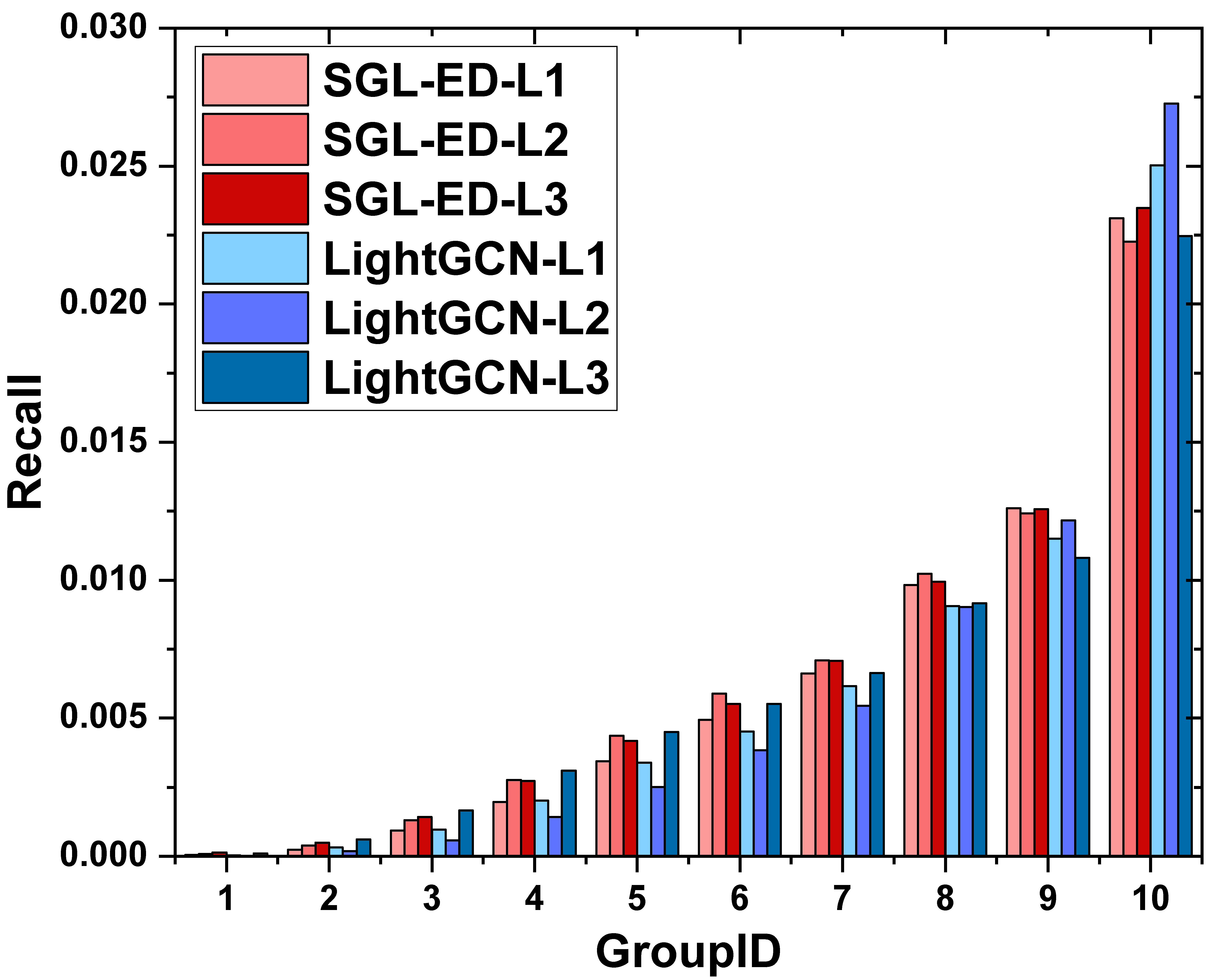
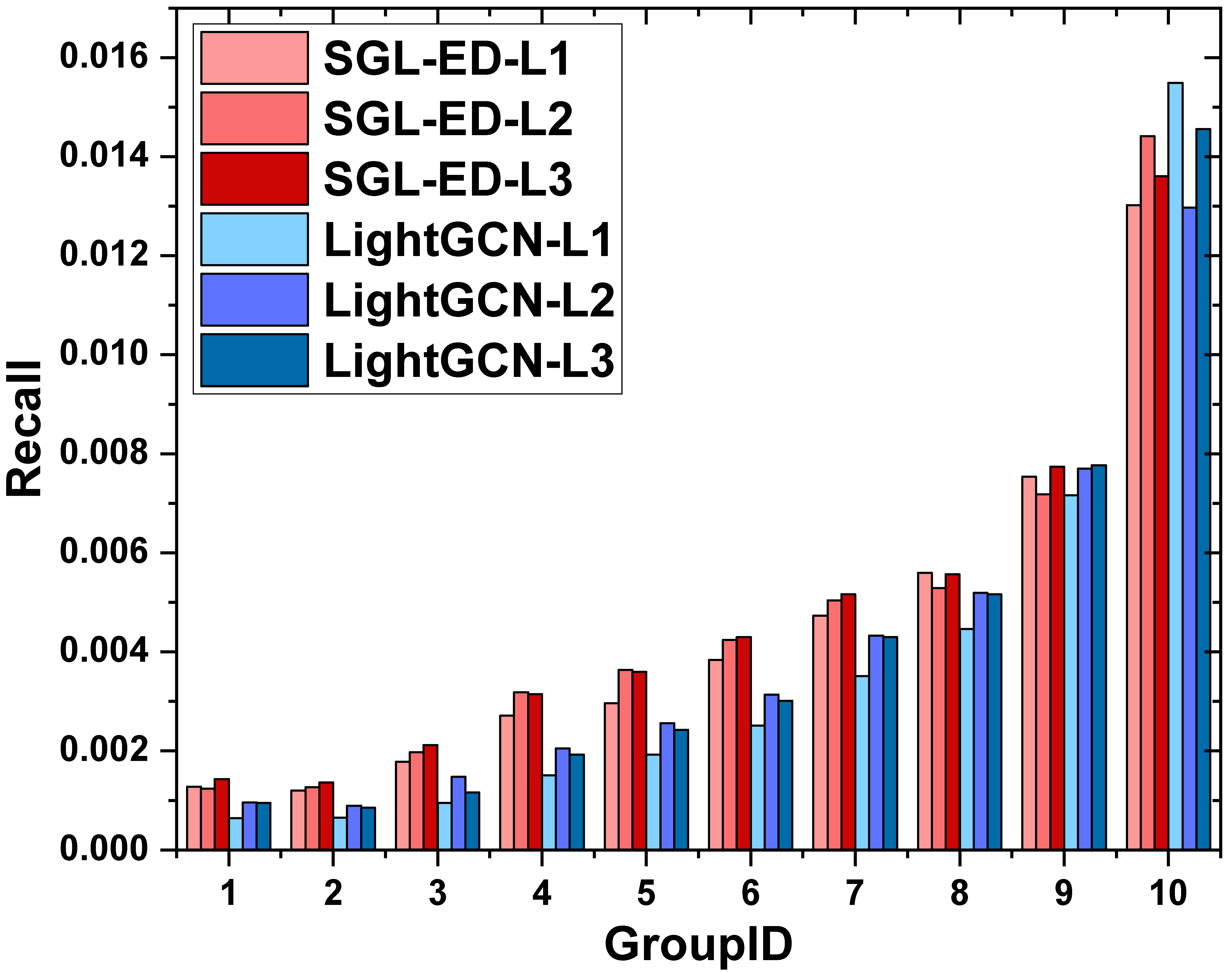
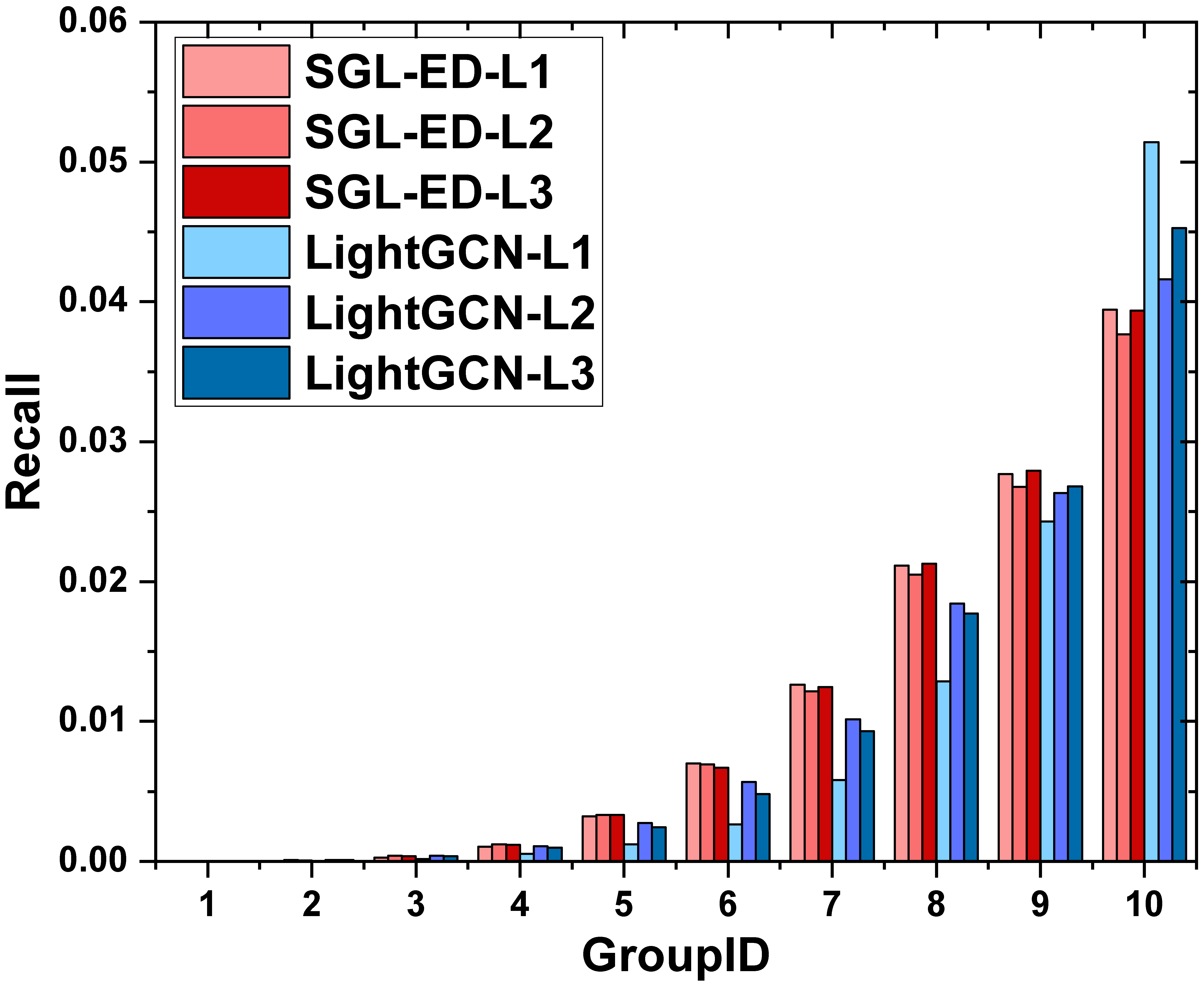
As Introduction mentions, GNN-based recommender models easily suffer from the long-tail problem. To verify whether SGL is of promise to solving the problem, we split items into ten groups based on the popularity, meanwhile keeping the total number of interactions of each group the same. The larger the GroupID is, the larger degrees the items have. We then decompose the Recall@20 metric of the whole dataset into contributions of single groups, as follows:
where is the number of users, and are the items in the top- recommendation list and relevant items in the testing set for user , respectively. As such, measures the recommendation performance over the -th group. We report the results in Figure 4 and find that:
-
•
LightGCN is inclined to recommend high-degree items, while leaving long-tail items less exposed. Specifically, although only containing 0.83%, 0.83% and 0.22% of item spaces, the 10-th group contributes 39.72%, 39.92% and 51.92% of the total Recall scores in three datasets, respectively. This admits that, LightGCN hardly learns high-quality representations of long-tail items, due to the sparse interaction signal. Our SGL shows potentials in alleviating this issue: the contributions of the 10-group downgrade to 36.27%, 29.15% and 35.07% in three datasets, respectively.
-
•
Jointly analyzing Table. 3 and Figure 4, we find the performance improvements of SGL mainly come from accurately recommending the items with sparse interactions. This again verifies that the representation learning benefits greatly from auxiliary supervisions, so as to establish better representations of these items than LightGCN.
4.3.2. Training Efficiency
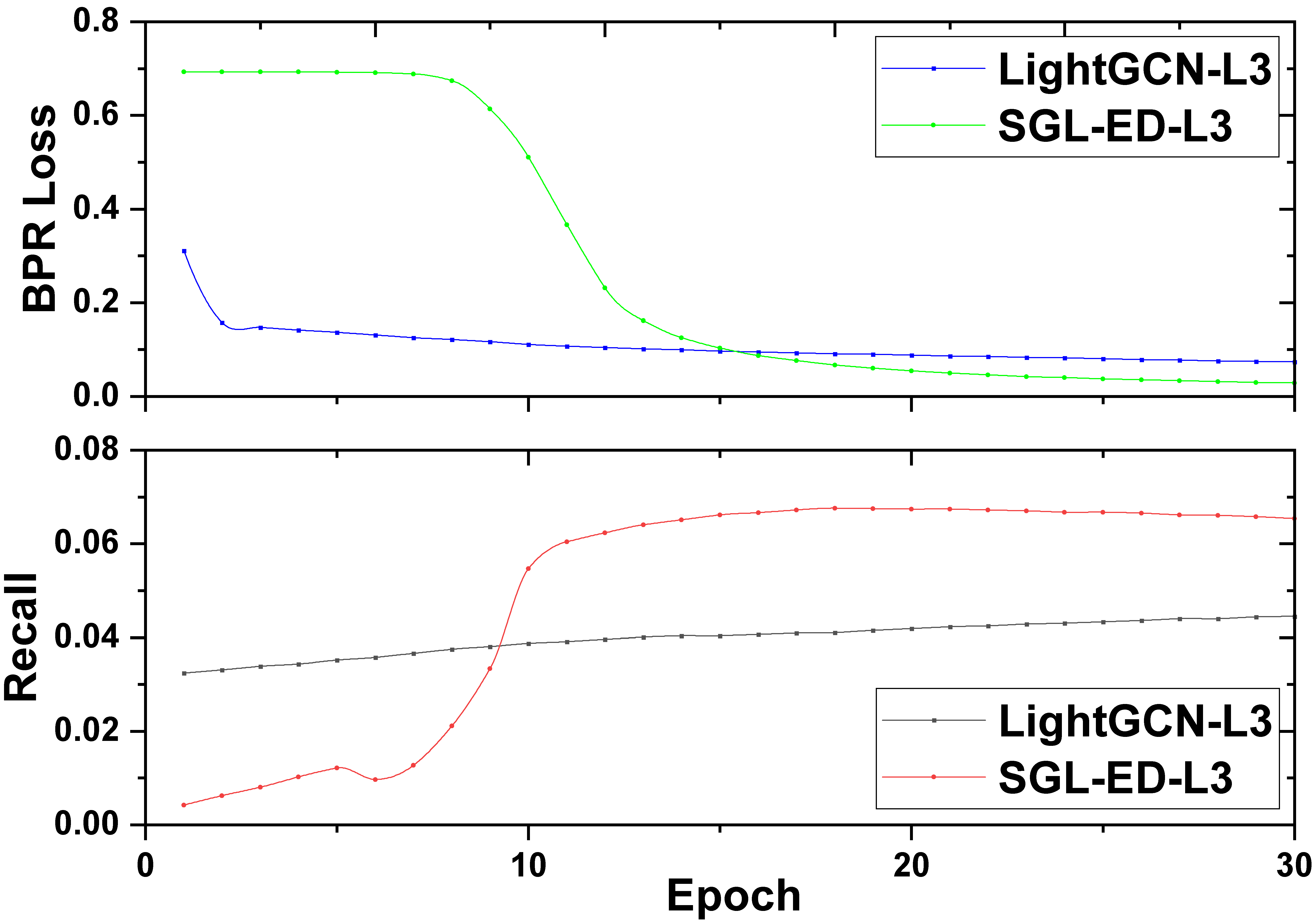
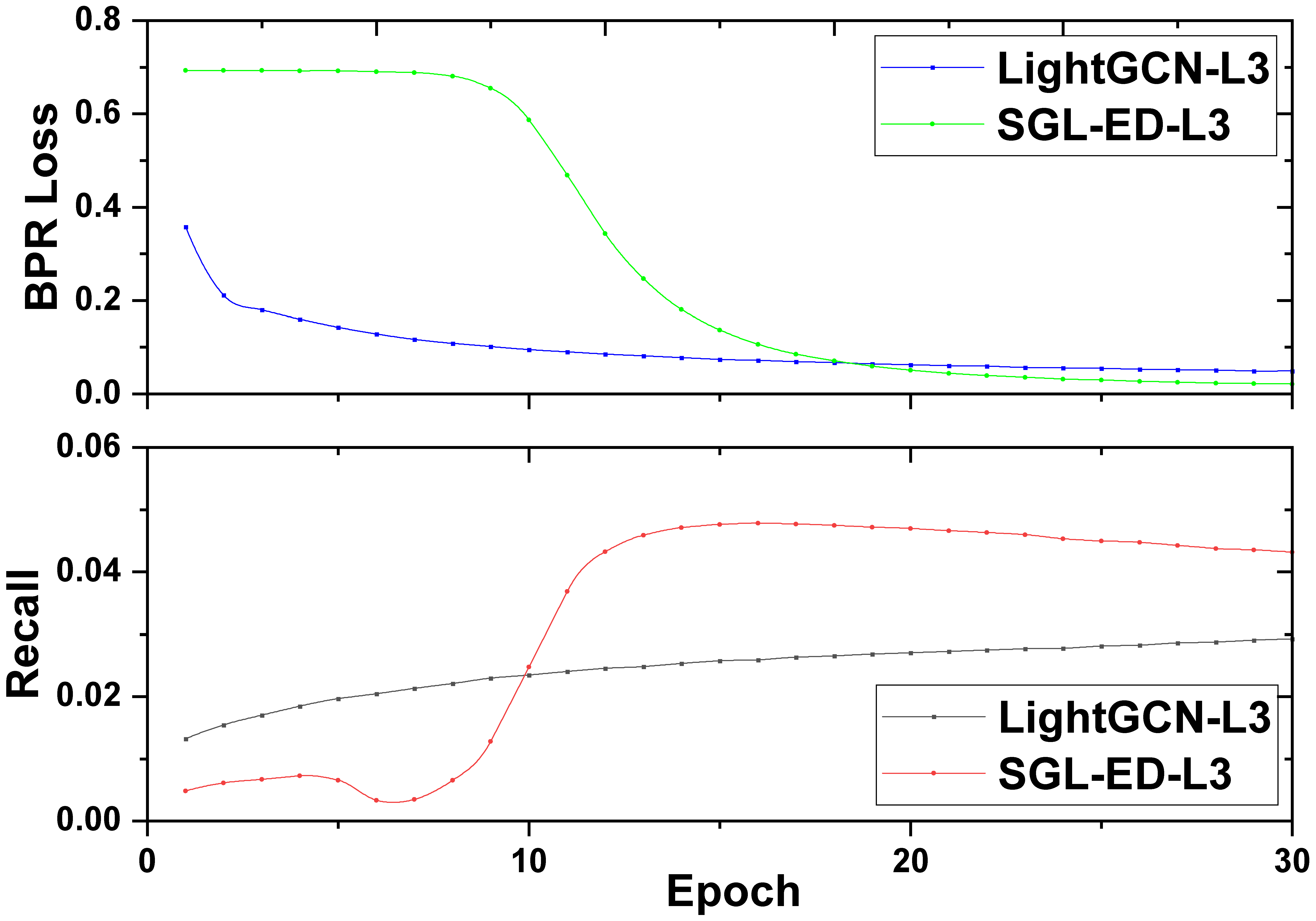
Self-supervised learning has proved its superiority in pre-training natural language model (Devlin et al., 2019) and graph structure (Qiu et al., 2020; Hu et al., 2020). Thus, we would like to study its influence on training efficiency. Figure 5 shows the training curves of SGL-ED and LightGCN on Yelp2018 and Amazon-Book. As the number of epochs increases, the upper subfigures display the changes of training loss, while the bottoms record the performance changes in the testing set. We have the following observations:
-
•
Obviously, SGL is much faster to converge than LightGCN on Yelp2018 and Amazon-Book. In particular, SGL arrives at the best performance at the 18-th and 16-th epochs, while LightGCN takes 720 and 700 epochs in these two datasets respectively. This suggests that our SGL can greatly reduce the training time, meanwhile achieves remarkable improvements. We ascribe such speedups to two factors: (1) SGL adopts the InfoNCE loss as the SSL objective which enables the model to learn representations from multiple negative samples, while the BPR loss in LightGCN only uses one negative sample which limits the model’s perception field; (2) As analyzed in Section 3.4, with a proper , SGL benefits from dynamic hard negative mining, where the hard negative samples offer meaningful and larger gradients to guide the optimization (Zhang et al., 2013).
-
•
Another observation is that the origin of the rapid-decline period of BPR loss is slightly later than the rapid-rising period of Recall. This indicates the existence of a gap between the BPR loss and ranking task. We will conduct in-depth research on this phenomenon in our future work.
4.3.3. Robustness to Noisy Interactions
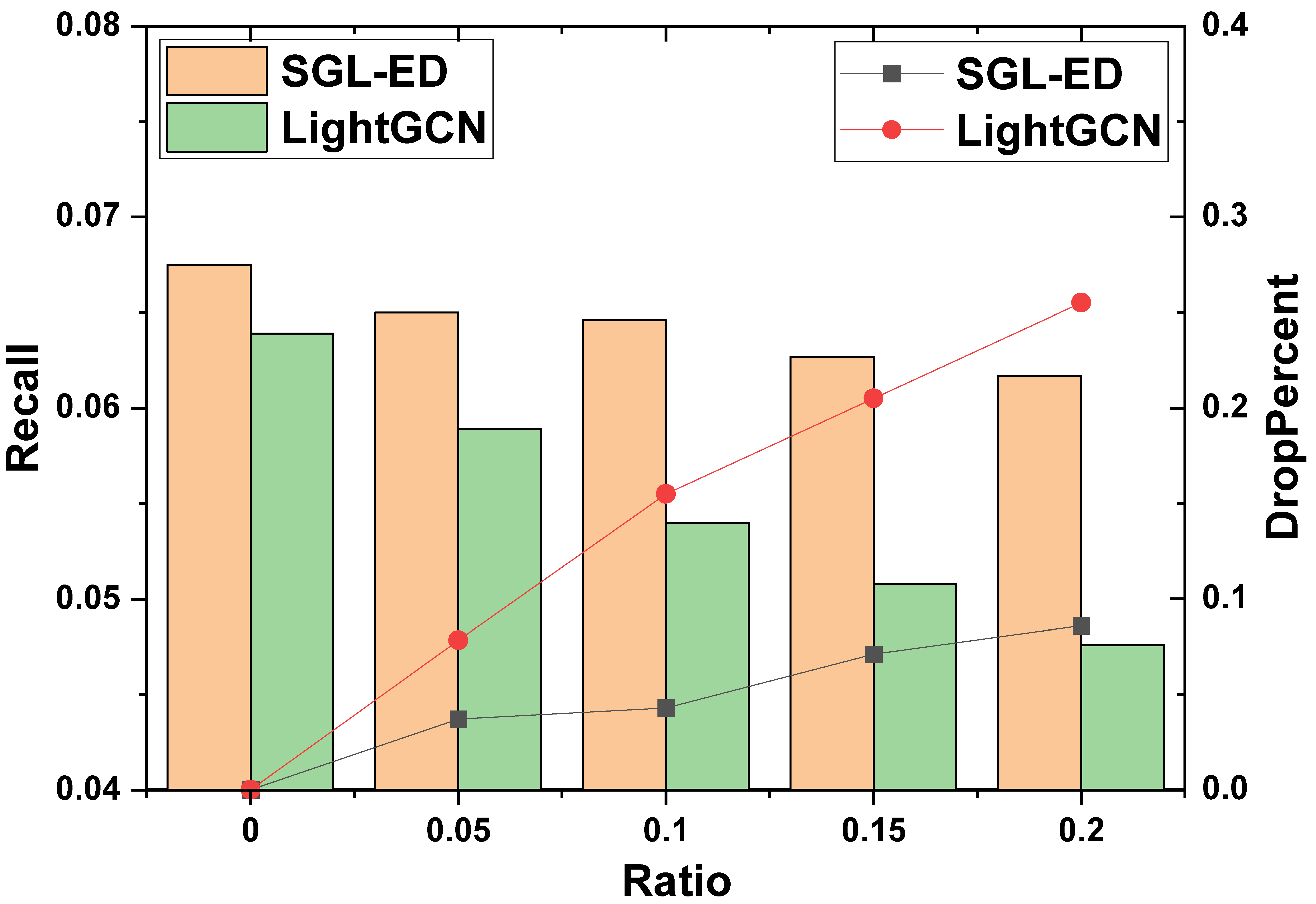
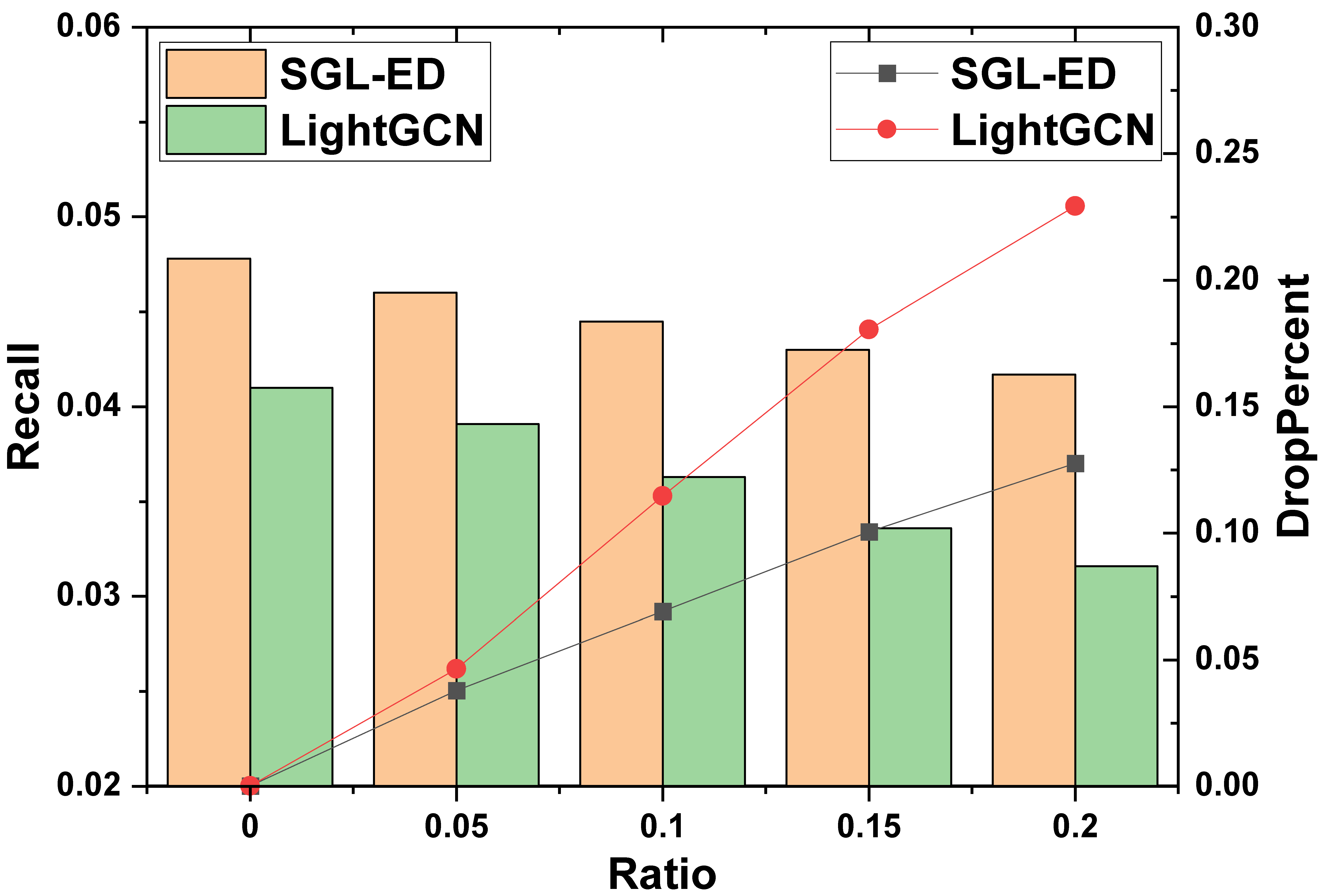
We also conduct experiments to check SGL’s robustness to noisy interactions. Towards this end, we contaminate the training set by adding a certain proportion of adversarial examples (i.e., 5%, 10%, 15%, 20% negative user-item interactions), while keeping the testing set unchanged. Figure 6 shows the results on Yelp2018 and Amazon-Book datasets.
-
•
Clearly, adding noise data reduces the performance of SGL and LightGCN. However, the performance degradation of SGL is lower than that of LightGCN; moreover, as the noise ratio increases, the gap between two degradation curves becomes more apparent. This suggests that, by comparing differently augmented views of nodes, SGL is able to figure out useful patterns, especially informative graph structures of nodes, and reduce dependence on certain edges. In a nutshell, SGL offers a different angle to denoise false positive interactions in recommendation.
-
•
Focusing on Amazon-Book, the performance of SGL with 20% additional noisy interactions is still superior to LightGCN with noise-free dataset. This further justifies the superiority and robustness of SGL over LightGCN.
-
•
We find that SGL is more robust on Yelp2018. The possible reason may be that Amazon-Book is much sparser than Yelp2018, and adding noisy data exerts more influence on graph structure of Amazon-Book than that of Yelp2018.
4.4. Study of SGL (RQ3)
| Dataset | Yelp2018 | Amazon-Book | ||
|---|---|---|---|---|
| Method | Recall | NDCG | Recall | NDCG |
| SGL-ED-batch | 0.0670 | 0.0549 | 0.0472 | 0.0374 |
| SGL-ED-merge | 0.0671 | 0.0547 | 0.0464 | 0.0368 |
| SGL-pre | 0.0653 | 0.0533 | 0.0429 | 0.0333 |
| SGL-ED | 0.0675 | 0.0555 | 0.0478 | 0.0379 |
We move on to studying different designs in SGL. We first investigate the impact of hyper-parameter . We then explore the potential of adopting SGL as a pretraining for existing graph-based recommendation model. Lastly, we study the influence of negatives in the SSL objective function. Due to the space limitation, we omit the results on iFashion which have a similar trend to that on Yelp2018 and Amazon-Book.
4.4.1. Effect of Temperature
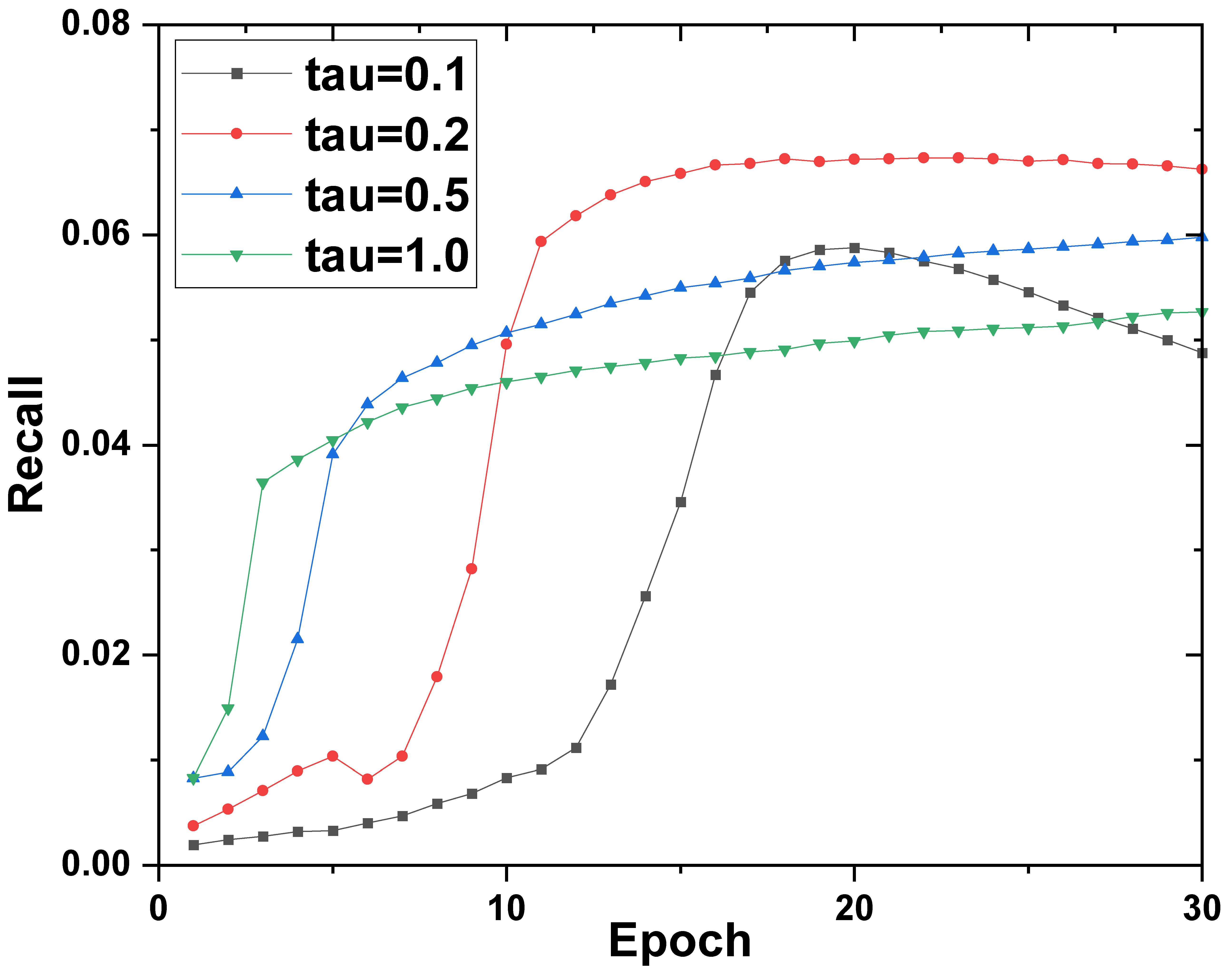
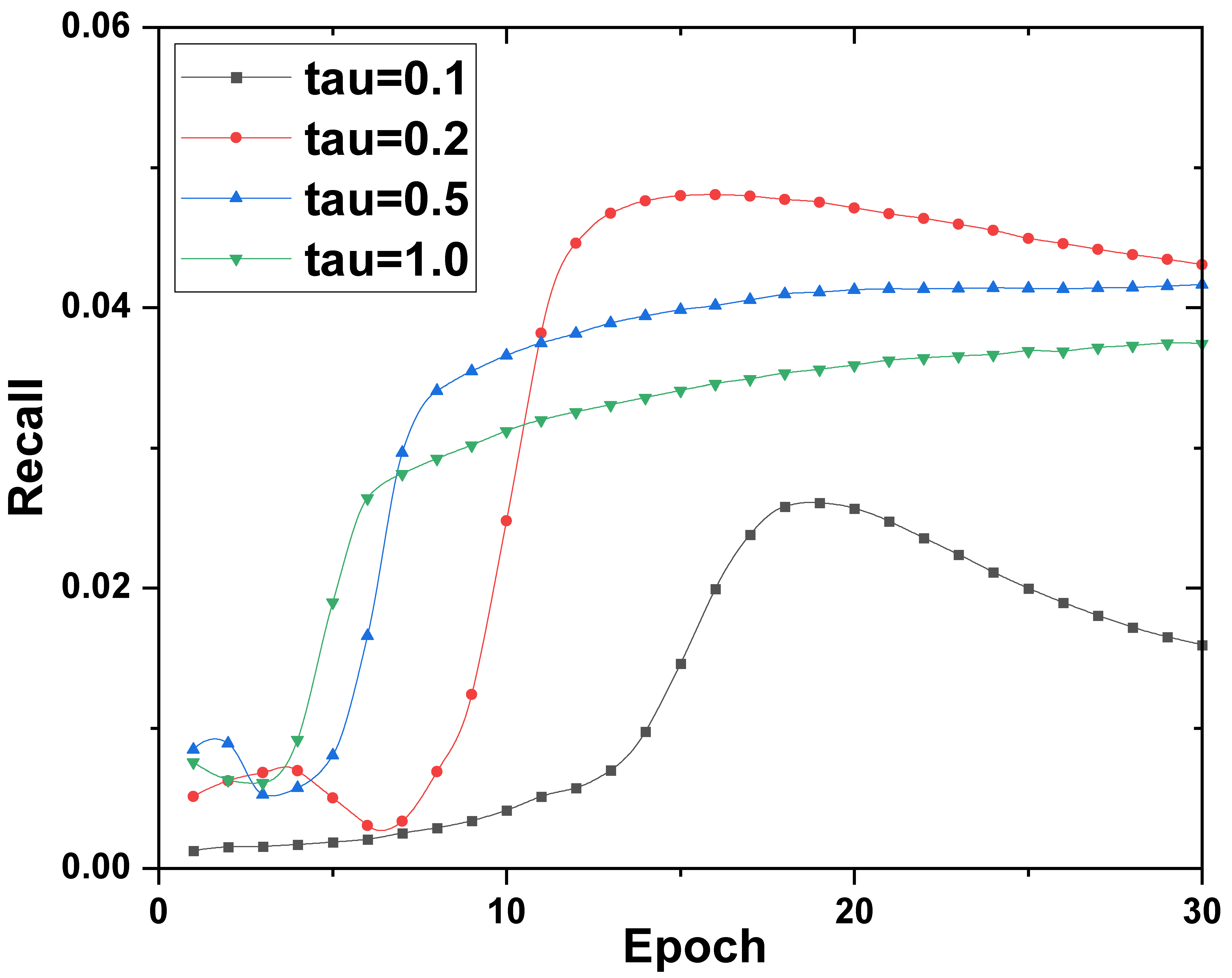
As verified in Section 3.4, play a critical role in hard negative mining. Figure 7 shows the curves of model performance w.r.t. different .
We can observe that: (1) Increasing the value of (e.g., 1.0) will lead to poorer performance and take more training epochs to converge, which fall short in the ability to distinguish hard negatives from easy negatives. (2) In contrast, fixing to a too small value (e.g., 0.1) will hurt the model performance, since the gradients of a few negatives dominate the optimization, losing the supremacy of adding multiple negative samples in the SSL objective. In a nutshell, we suggest to tun in the range of carefully.
4.4.2. Effect of Pre-training
The foregoing experiments have shown the effectiveness of SGL, where the main supervised task and the self-supervised task are jointly optimized. Here we would like to answer the question: Can the recommendation performance benefit from the pre-trained model? Towards this goal, we first pre-train the self-supervised task to obtain the model parameters, use them to initialize LightGCN, and then fine-tune the model via optimizing the main task. We term this variant as SGL-pre and show the comparison with SGL in Table 5. Clearly, although SGL-pre performs worse than SGL-ED on both datasets, the results of SGL-pre are still better than that of LightGCN (cf. Table 3). Our self-supervised task is able to offer a better initialization for LightGCN, which is consistent to the observation in previous studies (Chen et al., 2020b). However, the better performance of joint training admits that the representations in the main and auxiliary tasks are mutually enhanced with each other.
4.4.3. Effect of Negatives
Moreover, we also study the effect of the choice of negative samples in the auxiliary task. Two variants are considered: (1) SGL-ED-batch, which differentiates node types and treat users and items in a mini-batch as negative views for users and items, separately, and (2) SGL-ED-merge, which treat nodes within a mini-batch as negative, without differentiating the node types. We report the comparison in Table 5. SGL-ED-batch performs better than SGL-ED-merge, which indicates the necessity for distinguishing types of heterogeneous nodes. Moreover, SGL-ED-batch is on a par with SGL-ED that treats the whole spaces of users and items as negative. It suggests that training the SSL task in mini-batching is an efficient alternative.
5. Related Work
In this section, we separately review two tasks related to our work: graph-based recommendation and self-supervised learning.
5.1. Graph-based Recommendation
Previous studies on graph-based recommendation can be categorized into: model-level and graph-level methods, regarding their focus. The model-level methods focus on model design for mining the user-item graph. The research attention has evolved from the random walk that encodes the graph structure as transition probabilities (Baluja et al., 2008), to GCN that propagates user and item embeddings over the graph (van den Berg et al., 2017; Wang et al., 2019b; Ying et al., 2018; He et al., 2020a). Recently, attention mechanism is introduced into GCN-based recommendation models (Chen et al., 2019a), which learns to weigh the neighbors so as to capture the more informative user-item interactions. A surge of attention has also been dedicated to graph-level methods, which enriches the user-item graph by accounting for side information apart from user-item interactions, which ranges from user social relations (Bagci and Karagoz, 2016; Ren et al., 2017; Yuan et al., 2020), item co-occurrence (Baluja et al., 2008), to user and item attributes (Li et al., 2019). Recently, Knowledge Graph (KG) is also unified with the user-item graph, which enables considering the detailed types of linkage between items (Wang et al., 2019a; Cao et al., 2019; Wang et al., 2019c).
Despite the tremendous efforts devoted on these methods, all the existing work adopts the paradigm of supervised learning for model training. This work is in an orthogonal direction, which explores self-supervised learning, opening up a new research line of graph-based recommendation.
5.2. Self-supervised Learning
Studies on self-supervised learning can be roughly categorized into two branches: generative models (Mikolov et al., 2013; van den Oord et al., 2016; Devlin et al., 2019) and contrastive models (Gidaris et al., 2018; van den Oord et al., 2018; He et al., 2020b; Chen et al., 2020b). Auto-encoding is the most popular generative model which learns to reconstruct the input data, where noises can be intentionally added to enhance model robustness (Devlin et al., 2019). Contrastive models learn to compare through a Noise Contrastive Estimation (NCE) objective, which can be in either global-local contrast (Hjelm et al., 2019; van den Oord et al., 2018) or global-global contrast manner (Chen et al., 2020b; He et al., 2020b). The former focuses on modeling the relationship between the local part of a sample and its global context representation. While the latter directly performs comparison between different samples, which typically requires multiple views of samples (Tian et al., 2019; He et al., 2020b; Chen et al., 2020b). SSL has also been applied on graph data (You et al., 2020b; Zhu et al., 2020; You et al., 2020a). For instance, InfoGraph (Sun et al., 2020) and DGI (Velickovic et al., 2019) learns node representations according to mutual information between a node and the local structure. In addition, Hu et al. (Hu et al., 2020) extend the idea to learn GCN for graph representation. Furthermore, Kaveh et al. (Hassani and Khasahmadi, 2020) adopt the contrastive model for learning both node and graph representation, which contrasts node representations from one view with graph representation of another view. Besides, GCC (Qiu et al., 2020) leverages instance discrimination as the pretext task for graph structural information pre-training. These studies focused on general graphs while leaving the inherent properties of bipartite graph unconsidered.
To the best of our knowledge, very limited works exist in combining SSL with recommendation to date. A very recent one is -Rec (Zhou et al., 2020) for sequential recommendation which utilizes the mutual information maximization principle to learn the correlations among attribute, item, subsequence, and sequence. Another attempt (Yao et al., 2020) also adopts a multi-task framework with SSL. However, it differs from our work in: (1) (Yao et al., 2020) uses two-tower DNN as encoder, while our work sheds lights on graph-based recommendation, and devised three augmentation operators on graph structure. (2) (Yao et al., 2020) utilizes categorical metadata features as model input, while our work considers a more general collaborative filtering setting with only ID as feature.
6. Conclusion and Future Work
In this work, we recognized the limitations of graph-based recommendation under general supervised learning paradigm and explored the potential of SSL to solve the limitations. In particular, we proposed a model-agnostic framework SGL to supplement the supervised recommendation task with self-supervised learning on user-item graph. From the perspective of graph structure, we devised three types of data augmentation from different aspects to construct the auxiliary contrastive task. We conducted extensive experiments on three benchmark datasets, justifying the advantages of our proposal regarding long-tail recommendation, training convergence and robustness against noisy interactions.
This work represents an initial attempt to exploit self-supervised learning for recommendation and opens up new research possibilities. In future work, we would like to make SSL more entrenched with recommendation tasks. Going beyond the stochastic selections on graph structure, we plan to explore new perspectives, such as counterfactual learning to identify influential data points, to create more powerful data augmentations. Moreover, we will focus on pre-training and fine-tuning in recommendation, — that is, to pre-train a model which captures universal and transferable patterns of users across multiple domains or datasets, and fine-tune it on upcoming domains or datasets. Another promising direction is fulfilling the potential of SSL to address the long-tail issue. We hope the development of SGL is beneficial for improving the generalization and transferability of recommender models.
Acknowledgement. This work is supported by the National Natural Science Foundation of China (U19A2079, 61972372) and National Key Research and Development Program of China (2020AAA0106000).
References
- (1)
- Bagci and Karagoz (2016) Hakan Bagci and Pinar Karagoz. 2016. Context-Aware Friend Recommendation for Location Based Social Networks using Random Walk. In WWW. 531–536.
- Baluja et al. (2008) Shumeet Baluja, Rohan Seth, D. Sivakumar, Yushi Jing, Jay Yagnik, Shankar Kumar, Deepak Ravichandran, and Mohamed Aly. 2008. Video suggestion and discovery for youtube: taking random walks through the view graph. In WWW. 895–904.
- Bayer et al. (2017) Immanuel Bayer, Xiangnan He, Bhargav Kanagal, and Steffen Rendle. 2017. A Generic Coordinate Descent Framework for Learning from Implicit Feedback. In WWW. 1341–1350.
- Cao et al. (2019) Yixin Cao, Xiang Wang, Xiangnan He, Zikun Hu, and Tat-Seng Chua. 2019. Unifying Knowledge Graph Learning and Recommendation: Towards a Better Understanding of User Preferences. In WWW. 151–161.
- Chen et al. (2020a) Jiawei Chen, Hande Dong, Xiang Wang, Fuli Feng, Meng Wang, and Xiangnan He. 2020a. Bias and Debias in Recommender System: A Survey and Future Directions. CoRR abs/2010.03240 (2020).
- Chen et al. (2020b) Ting Chen, Simon Kornblith, Mohammad Norouzi, and Geoffrey E. Hinton. 2020b. A Simple Framework for Contrastive Learning of Visual Representations. CoRR abs/2002.05709 (2020).
- Chen et al. (2019a) Weijian Chen, Yulong Gu, Zhaochun Ren, Xiangnan He, Hongtao Xie, Tong Guo, Dawei Yin, and Yongdong Zhang. 2019a. Semi-supervised User Profiling with Heterogeneous Graph Attention Networks. In IJCAI. 2116–2122.
- Chen et al. (2019b) Wen Chen, Pipei Huang, Jiaming Xu, Xin Guo, Cheng Guo, Fei Sun, Chao Li, Andreas Pfadler, Huan Zhao, and Binqiang Zhao. 2019b. POG: Personalized Outfit Generation for Fashion Recommendation at Alibaba iFashion. In SIGKDD. 2662–2670.
- Clauset et al. (2009) Aaron Clauset, Cosma Rohilla Shalizi, and Mark E. J. Newman. 2009. Power-Law Distributions in Empirical Data. SIAM 51, 4 (2009), 661–703.
- Devlin et al. (2019) Jacob Devlin, Ming-Wei Chang, Kenton Lee, and Kristina Toutanova. 2019. BERT: Pre-training of Deep Bidirectional Transformers for Language Understanding. In NAACL-HLT. 4171–4186.
- Gidaris et al. (2018) Spyros Gidaris, Praveer Singh, and Nikos Komodakis. 2018. Unsupervised Representation Learning by Predicting Image Rotations. In ICLR.
- Gilmer et al. (2017) Justin Gilmer, Samuel S. Schoenholz, Patrick F. Riley, Oriol Vinyals, and George E. Dahl. 2017. Neural Message Passing for Quantum Chemistry. In ICML, Vol. 70. 1263–1272.
- Glorot and Bengio (2010) Xavier Glorot and Yoshua Bengio. 2010. Understanding the difficulty of training deep feedforward neural networks. In AISTATS, Vol. 9. 249–256.
- Gutmann and Hyvärinen (2010) Michael Gutmann and Aapo Hyvärinen. 2010. Noise-contrastive estimation: A new estimation principle for unnormalized statistical models. In AISTATS, Vol. 9. 297–304.
- Hamilton et al. (2017) William L. Hamilton, Zhitao Ying, and Jure Leskovec. 2017. Inductive Representation Learning on Large Graphs. In NeurIPS. 1024–1034.
- Hassani and Khasahmadi (2020) Kaveh Hassani and Amir Hosein Khasahmadi. 2020. Contrastive Multi-View Representation Learning on Graphs. In ICML. 3451–3461.
- He et al. (2020b) Kaiming He, Haoqi Fan, Yuxin Wu, Saining Xie, and Ross B. Girshick. 2020b. Momentum Contrast for Unsupervised Visual Representation Learning. In CVPR. 9726–9735.
- He and McAuley (2016) Ruining He and Julian J. McAuley. 2016. Ups and Downs: Modeling the Visual Evolution of Fashion Trends with One-Class Collaborative Filtering. In WWW. 507–517.
- He et al. (2020a) Xiangnan He, Kuan Deng, Xiang Wang, Yan Li, Yong-Dong Zhang, and Meng Wang. 2020a. LightGCN: Simplifying and Powering Graph Convolution Network for Recommendation. In SIGIR. 639–648.
- He et al. (2018) Xiangnan He, Zhankui He, Jingkuan Song, Zhenguang Liu, Yu-Gang Jiang, and Tat-Seng Chua. 2018. NAIS: Neural Attentive Item Similarity Model for Recommendation. TKDE 30, 12 (2018), 2354–2366.
- He et al. (2017) Xiangnan He, Lizi Liao, Hanwang Zhang, Liqiang Nie, Xia Hu, and Tat-Seng Chua. 2017. Neural Collaborative Filtering. In WWW. 173–182.
- Hjelm et al. (2019) R. Devon Hjelm, Alex Fedorov, Samuel Lavoie-Marchildon, Karan Grewal, Philip Bachman, Adam Trischler, and Yoshua Bengio. 2019. Learning deep representations by mutual information estimation and maximization. In ICLR.
- Hu et al. (2020) Weihua Hu, Bowen Liu, Joseph Gomes, Marinka Zitnik, Percy Liang, Vijay S. Pande, and Jure Leskovec. 2020. Strategies for Pre-training Graph Neural Networks. In ICLR.
- Khosla et al. (2020) Prannay Khosla, Piotr Teterwak, Chen Wang, Aaron Sarna, Yonglong Tian, Phillip Isola, Aaron Maschinot, Ce Liu, and Dilip Krishnan. 2020. Supervised Contrastive Learning. In NeurIPS.
- Koren (2008) Yehuda Koren. 2008. Factorization meets the neighborhood: a multifaceted collaborative filtering model. In KDD. 426–434.
- Lan et al. (2020) Zhenzhong Lan, Mingda Chen, Sebastian Goodman, Kevin Gimpel, Piyush Sharma, and Radu Soricut. 2020. ALBERT: A Lite BERT for Self-supervised Learning of Language Representations. In ICLR.
- Li et al. (2019) Zekun Li, Zeyu Cui, Shu Wu, Xiaoyu Zhang, and Liang Wang. 2019. Fi-GNN: Modeling Feature Interactions via Graph Neural Networks for CTR Prediction. In CIKM. 539–548.
- Liang et al. (2018) Dawen Liang, Rahul G. Krishnan, Matthew D. Hoffman, and Tony Jebara. 2018. Variational Autoencoders for Collaborative Filtering. In WWW. 689–698.
- Mikolov et al. (2013) Tomas Mikolov, Ilya Sutskever, Kai Chen, Gregory S. Corrado, and Jeffrey Dean. 2013. Distributed Representations of Words and Phrases and their Compositionality. In NIPS. 3111–3119.
- Milojevic (2010) Stasa Milojevic. 2010. Power law distributions in information science: Making the case for logarithmic binning. J. Assoc. Inf. Sci. Technol. 61, 12 (2010), 2417–2425.
- Qiu et al. (2020) Jiezhong Qiu, Qibin Chen, Yuxiao Dong, Jing Zhang, Hongxia Yang, Ming Ding, Kuansan Wang, and Jie Tang. 2020. GCC: Graph Contrastive Coding for Graph Neural Network Pre-Training. In KDD. 1150–1160.
- Ren et al. (2017) Zhaochun Ren, Shangsong Liang, Piji Li, Shuaiqiang Wang, and Maarten de Rijke. 2017. Social Collaborative Viewpoint Regression with Explainable Recommendations. In WSDM. 485–494.
- Rendle and Freudenthaler (2014) Steffen Rendle and Christoph Freudenthaler. 2014. Improving pairwise learning for item recommendation from implicit feedback. In WSDM. 273–282.
- Rendle et al. (2009) Steffen Rendle, Christoph Freudenthaler, Zeno Gantner, and Lars Schmidt-Thieme. 2009. BPR: Bayesian Personalized Ranking from Implicit Feedback. In UAI. 452–461.
- Sun et al. (2020) Fan-Yun Sun, Jordan Hoffmann, Vikas Verma, and Jian Tang. 2020. InfoGraph: Unsupervised and Semi-supervised Graph-Level Representation Learning via Mutual Information Maximization. In ICLR.
- Tang et al. (2020) Xianfeng Tang, Huaxiu Yao, Yiwei Sun, Yiqi Wang, Jiliang Tang, Charu Aggarwal, Prasenjit Mitra, and Suhang Wang. 2020. Investigating and Mitigating Degree-Related Biases in Graph Convolutional Networks. In CIKM.
- Tian et al. (2019) Yonglong Tian, Dilip Krishnan, and Phillip Isola. 2019. Contrastive Multiview Coding. CoRR abs/1906.05849 (2019).
- van den Berg et al. (2017) Rianne van den Berg, Thomas N. Kipf, and Max Welling. 2017. Graph Convolutional Matrix Completion. CoRR abs/1706.02263 (2017).
- van den Oord et al. (2016) Aäron van den Oord, Nal Kalchbrenner, Lasse Espeholt, Koray Kavukcuoglu, Oriol Vinyals, and Alex Graves. 2016. Conditional Image Generation with PixelCNN Decoders. In NIPS. 4790–4798.
- van den Oord et al. (2018) Aäron van den Oord, Yazhe Li, and Oriol Vinyals. 2018. Representation Learning with Contrastive Predictive Coding. CoRR abs/1807.03748 (2018).
- Velickovic et al. (2018) Petar Velickovic, Guillem Cucurull, Arantxa Casanova, Adriana Romero, Pietro Liò, and Yoshua Bengio. 2018. Graph Attention Networks. In ICLR.
- Velickovic et al. (2019) Petar Velickovic, William Fedus, William L. Hamilton, Pietro Liò, Yoshua Bengio, and R. Devon Hjelm. 2019. Deep Graph Infomax. In ICLR.
- Wang et al. (2019c) Hongwei Wang, Miao Zhao, Xing Xie, Wenjie Li, and Minyi Guo. 2019c. Knowledge Graph Convolutional Networks for Recommender Systems. In WWW. 3307–3313.
- Wang et al. (2021) Wenjie Wang, Fuli Feng, Xiangnan He, Liqiang Nie, and Tat-Seng Chua. 2021. Denoising Implicit Feedback for Recommendation. In WSDM.
- Wang et al. (2019a) Xiang Wang, Xiangnan He, Yixin Cao, Meng Liu, and Tat-Seng Chua. 2019a. KGAT: Knowledge Graph Attention Network for Recommendation. In SIGKDD. 950–958.
- Wang et al. (2019b) Xiang Wang, Xiangnan He, Meng Wang, Fuli Feng, and Tat-Seng Chua. 2019b. Neural Graph Collaborative Filtering. In SIGIR. 165–174.
- Wu et al. (2018) Zhirong Wu, Yuanjun Xiong, Stella X. Yu, and Dahua Lin. 2018. Unsupervised Feature Learning via Non-Parametric Instance Discrimination. In CVPR. 3733–3742.
- Xu et al. (2019) Keyulu Xu, Weihua Hu, Jure Leskovec, and Stefanie Jegelka. 2019. How Powerful are Graph Neural Networks?. In ICLR.
- Yao et al. (2020) Tiansheng Yao, Xinyang Yi, Derek Zhiyuan Cheng, Felix X. Yu, Aditya Krishna Menon, Lichan Hong, Ed H. Chi, Steve Tjoa, Jieqi Kang, and Evan Ettinger. 2020. Self-supervised Learning for Deep Models in Recommendations. CoRR abs/2007.12865 (2020).
- Ying et al. (2018) Rex Ying, Ruining He, Kaifeng Chen, Pong Eksombatchai, William L. Hamilton, and Jure Leskovec. 2018. Graph Convolutional Neural Networks for Web-Scale Recommender Systems. In KDD. 974–983.
- You et al. (2020a) Yuning You, Tianlong Chen, Yongduo Sui, Ting Chen, Zhangyang Wang, and Yang Shen. 2020a. Graph Contrastive Learning with Augmentations. In NeurIPS.
- You et al. (2020b) Yuning You, Tianlong Chen, Zhangyang Wang, and Yang Shen. 2020b. When Does Self-Supervision Help Graph Convolutional Networks?. In ICML, Vol. 119. 10871–10880.
- Yuan et al. (2020) Fajie Yuan, Xiangnan He, Alexandros Karatzoglou, and Liguang Zhang. 2020. Parameter-efficient transfer from sequential behaviors for user modeling and recommendation. In SIGIR. 1469–1478.
- Zhang et al. (2013) Weinan Zhang, Tianqi Chen, Jun Wang, and Yong Yu. 2013. Optimizing top-n collaborative filtering via dynamic negative item sampling. In SIGIR. 785–788.
- Zhou et al. (2020) Kun Zhou, Hui Wang, Wayne Xin Zhao, Yutao Zhu, Sirui Wang, Fuzheng Zhang, Zhongyuan Wang, and Ji-Rong Wen. 2020. S^3-Rec: Self-Supervised Learning for Sequential Recommendation with Mutual Information Maximization. In CIKM.
- Zhu et al. (2020) Yanqiao Zhu, Yichen Xu, Feng Yu, Qiang Liu, Shu Wu, and Liang Wang. 2020. Graph Contrastive Learning with Adaptive Augmentation. CoRR abs/2010.14945 (2020).
Appendix A Gradient of InfoNCE Loss w.r.t. node representation
Here we derive the Equation (12). Since we adopt cosine similarity function in the contrastive loss, we here decouple the normalization to show its superiority inspired from (Khosla et al., 2020). For a user , the contrastive loss is as follows:
| (18) |
where and are the normalized representations, i.e., . The gradient of the contrastive Loss w.r.t. can be calculated via the chain rule of scalar-by-vector:
| (19) |
where,
| (20) | ||||
| (21) | ||||
where,
| (22) | ||||
| (23) |
is the likelihood for w.r.t. all samples within . Therefore, we have
| (24) | ||||