ASCII: ASsisted Classification with
Ignorance Interchange

Abstract

The rapid development in data collecting devices and computation platforms produces an emerging number of agents, each equipped with a unique data modality over a particular population of subjects. While an agent’s predictive performance may be enhanced by transmitting others’ data to it, this is often unrealistic due to intractable transmission costs and security concerns. In this paper, we propose a method named ASCII for an agent to improve its classification performance through assistance from other agents. The main idea is to iteratively interchange an ignorance value between 0 and 1 for each collated sample among agents, where the value represents the urgency of further assistance needed. The method is naturally suitable for privacy-aware, transmission-economical, and decentralized learning scenarios. The method is also general as it allows the agents to use arbitrary classifiers such as logistic regression, ensemble tree, and neural network, and they may be heterogeneous among agents. We demonstrate the proposed method with extensive experimental studies.

I Introduction

In recent years, the advancement of mobile devices and information technology has led to an emerging number of distributed multimodal data sources for different populations, e.g., a group of patients and a cohort of mobile users [1]. Each source of data is often collected and held by an agent with domain-specific interest. For example, suppose that agent A is a grocery store that aims to predict customers’ shopping preferences using its shopping records, and agent B is an IT service company with the customers’ mobile data. Both A and B hold a unique set of features from the same population. In other words, they hold two submatrices of a holistic data matrix (in hindsight) where rows are indexed by customer IDs. Intuitively, if Agent A can build a model based on the holistic data matrix, the prediction performances would typically be better than model trained only with A’s data.

However, constructing such a holistic matrix may give rise to certain problems, e.g., breach of data privacy [2, 3, 4, 5, 6, 7], infeasible transmission cost [8, 9], and hardware capacity [10, 11]. Moreover, data fusion often assumes a centralized dataset held by one agent [12]. The above challenges motivate the following question. Can any particular agent improve its learning quality with the assistance of other agents, but without transmitting their private data or models? In this paper, we present a general solution named ASsisted Classification with Ignorance Interchange (ASCII), to address the above challenge. The ASCII allows each agent to assist other agents by interchanging communication-efficient statistics instead of raw data. Consequently, such assistance enables a significantly better performance compared with single-agent learning (without assistance). Such assistance will also allow agents to use their own private models (or algorithms) and data modality.

A related work is Federated Learning (FL) [13, 14, 15], which is a distributed learning framework that features communication efficiency. The main idea of FL to learn a joint model using the averaging of locally learned model parameters, so that the training data do not need to be transmitted. To address heterogeneous data, there exist some recent work of vertically-partitioned FL, including those based on the homomorphic encryption and partial stochastic gradient descent [16, 17, 18, 19]. While FL agents are required to use a commonly shared global model, our assisted learning allows agents to autonomously use their own (private) models as well as data.

The main idea of our method is described as follows. First, we let A fit its model, and then evaluate the model on each sample to obtain an ‘ignorance’ score, which is a value between 0 and 1 indicating the extent to which a sample may not be ignored. A substantial ignorance score (say 1) means that the corresponding sample has not been adequately modeled, and thus extra information is needed from other agents. Second, A sends the labels and ignorance scores to B, who uses its data and model to train a classifier using weighted samples. Here, B’s sample weights will be the current ignorance scores so that B can focus on those data that have not been well-modeled before. After that, B updates the ignorance scores and sends them back to A, who will then initialize the second round of information interchange. The above interactions are repeated until a stop criterion is met. For future inference, B will apply an ensemble model created from its local models (when interacting with A) to its new data observation and sends the prediction result to A. A will then integrate it with its prediction result to make the final decision. In this way, B provides side information to A to eventually improve A’s learning task. Note that the above learning mechanism only needs A and B to exchange numerical labels (for local training), data IDs (for data collation), and ignorance scores (for side information), instead of raw data. Moreover, agents are free to use their own learning models. In the above procedure, the ignorance scores are mathematically derived so that the final classifier of A as assisted from B will approximate the oracle classifier using the hypothetically collated data from A and B.

Our derivation of the algorithm was inspired by the pioneering work of Adaptive Boosting (AdaBoost) [20, 21, 22, 23], where weak learners are sequentially created and aggregated into a strong learner. Like AdaBoost, our approach will also create a sequence of models trained from weighted samples. The main difference between AdaBoost and our method is two folds. First, AdaBoost performs training on all the data, while our approach is based on training heterogeneous data held by different agents. Second, in our approach, each agent’s sample weights are calculated from both the agent’s previous sample weights and other agents’ transmitted weights (‘ignorance’). Our method may be regarded as a generalization of AdaBoost to address privacy-aware distributed learning with vertically-split variables.

The main contributions of this work are three folds. First, we propose an assisted learning method where an agent can significantly improve its learning performance by interchanging side information with other agents, without transmitting private data or private models. Second, we establish the method in a general ‘model-free’ framework, meaning that we allow each agent to employ its own model. As a result, agents do not necessarily use the same global model or a trusted third party for coordination, appealing in many autonomous learning scenarios. Third, we develop theoretical justifications and interpretations of the derived ignorance scores. We show by extensive experiments that the proposed solution will significantly enhance single-agent learning performance. Moreover, in many cases, the method also produces near-oracle performance, where the oracle is defined as the performance from hypothetically collated dataset.

The outline of the paper is given below. In Section II, we introduce some notation and formulate the problem. In Section III, we propose a general approach for assisted classification in a two-agent scenario and discuss its theoretical justifications. In Section IV, we extend the proposed method to a multi-agent scenario. In Section V, we introduce some variants of the proposed algorithm, and highlight the unique advantages of our proposal in later numerical comparisons. We provide extensive experimental studies in Section VI, and conclude the work in Section VII.

II Problem

II-A Background and Notation

We first introduce some notation. Suppose there exist $M$ agents, and the $m$-th agent holds $\mathbf{X}^{(m)}=[\mathbf{x}_{1}^{(m)},\ldots,\mathbf{x}_{n}^{(m)}]^{\mathrm{\scriptscriptstyle T}}\in\mathbb{R}^{n\times p_{m}}$ as the private data matrix, where $n$ is the sample size and $p_{m}$ is the number of feature variables, $m=1,\ldots,M$. We will consider a classification problem that involves $K$ classes ($K\geq 2$). Let $\mathbf{c}=[c_{1},c_{2},\ldots,c_{n}]^{\mathrm{\scriptscriptstyle T}}$ denote the $K$-class label vector accessible by all the agents, where $c_{i}\in\{1,2,\ldots,K\}$. Suppose that when the agents exchange information, they have a consensus on how to collate/align the data through a certain sample ID (e.g., person ID or timestamp). In the above setup, we implicitly assumed that their data could be collated and features are non-overlapping. If the data are partially overlapping (in terms of sample ID), we suppose that only the overlapping data are used for technical convenience. To develop our technical approach, we will re-code the label vector $\mathbf{c}$ into a label matrix $\mathbf{Y}=[\mathbf{y}_{1},\mathbf{y}_{2},\ldots,\mathbf{y}_{n}]^{\mathrm{\scriptscriptstyle T}}$, where each row $\mathbf{y}_{i}=[y_{i1},y_{i2},\ldots,y_{iK}]^{\mathrm{\scriptscriptstyle T}}$ with

$$y_{ij}=\left\{\begin{array}[]{cc}1&c_{i}=j\\ -\frac{1}{K-1}&c_{i}\neq j\\ \end{array}\right.$$ (1)

encodes the class $c_{i}$. Let $\mathcal{X}^{(m)}$ and $\mathcal{Y}$ denote the feature space of agent $m$ and label space, respectively. The main reason we use this encoding method is for technical convenience when implementing the exponential loss that we will elaborate in Section II-B. The above code format has been widely used, for multi-class classification tasks, e.g., support vector machines [24] and boosting [23].

II-B Problem Formulation

II-B1 Adaboost for the single-agent case

Before we introduce the formulation for multi-agent assisted learning, we briefly review the framework of single-agent learning and the AdaBoost algorithm for it.

Suppose that an agent is equipped with a data matrix $\mathbf{X}=[\mathbf{x}_{1},\ldots,\mathbf{x}_{n}]^{\mathrm{\scriptscriptstyle T}}$ and classification label matrix $\mathbf{Y}=[\mathbf{y}_{1},\ldots,\mathbf{y}_{n}]^{\mathrm{\scriptscriptstyle T}}$. Note that $\mathbf{y}_{i}$ re-codes class $c_{i}$ into a length-$K$ vector. The supervised learning task is to find a function $\mathbf{f}(\mathbf{x})=[f_{1}(\mathbf{x}),f_{2}(\mathbf{x}),\ldots,f_{K}(\mathbf{x})]^{\mathrm{\scriptscriptstyle T}}$ that approximates the function relationship between $\mathbf{X}$ and $\mathbf{Y}$. In many statistical learning contexts, the $\mathbf{f}$ is usually estimated by a risk minimization problem in the form of

$$\min_{\mathbf{f}\in\mathcal{F}_{T}}\sum_{i=1}^{n}\ell(\mathbf{y}_{i},\mathbf{f}(\mathbf{x}_{i})),$$ (2)

$$\text{subject to}\quad f_{1}(\mathbf{x})+\ldots+f_{K}(\mathbf{x})=0,$$

where $\ell$ and $\mathcal{F}_{T}$ are appropriately chosen loss function and model class, respectively. For a future (or testing) data $\tilde{\mathbf{x}}$, the learned model produces a prediction $\tilde{\mathbf{y}}$ that corresponds to the prediction label $\tilde{c}=\operatorname*{arg\,max}_{i}f_{i}(\tilde{\mathbf{x}})$. Note that the above constraint is to ensure the identifiability of $\mathbf{f}$.

The AdaBoost algorithm [20, 21, 22, 23] is derived based on a specific loss function and a model class. In particular, it uses the following exponential loss function,

$$\ell:(\mathbf{y},\mathbf{f})\mapsto e^{-\frac{1}{K}\mathbf{y}^{\mathrm{\scriptscriptstyle T}}\mathbf{f}},$$

and the following model class (also referred to as ‘additive models’),

$$\mathcal{F}_{T}=\biggl{\{}\mathbf{f}:\mathbf{f}(\mathbf{x})=\sum_{t=1}^{T}\alpha_{t}\mathbf{g}_{t}(\mathbf{x}),\,\alpha_{t}\in\mathbb{R},\,\mathbf{g}_{t}\in\mathcal{F}_{0}\biggr{\}}.$$

where $T$ is the number of weak learners, and $\mathcal{F}_{0}$ is a class of basis functions mapping from $\mathcal{X}$ to $\mathcal{Y}$ (e.g., decision trees and linear classifiers), and $\alpha_{t}$ and $\mathbf{g}_{t}$, $t=1,\ldots,T$ are the unknown parameters/functions.

The vector form of $\mathbf{f}(\mathbf{x})$ as derived by [23] implies that given $\mathbf{x}$, $\mathbf{g}_{t}(\mathbf{x})$ maps $\mathbf{x}$ onto $\mathcal{Y}$:

$$\mathbf{g}_{t}:\mathbf{x}\in\mathbb{R}^{p}\mapsto\mathcal{Y},$$

where

$$\mathcal{Y}=\left\{\begin{array}[]{cccc}(1,-\frac{1}{K-1},-\frac{1}{K-1},\ldots,-\frac{1}{K-1})\\ (-\frac{1}{K-1},1,-\frac{1}{K-1},\ldots,-\frac{1}{K-1})\\ \vdots\\ (-\frac{1}{K-1},-\frac{1}{K-1},-\frac{1}{K-1},\ldots,1)\\ \end{array}\right\}$$ (7)

is the collection of all such label vectors in (1).

What remains in (2) is to determine the weak classifier $\mathbf{g}_{t}$ and what its weight $\alpha_{t}$ should be. Under the forward stage-wise optimization framework, at iteration $t$, $\mathbf{g}_{t}$ and $\alpha_{t}$ are optimized individually, and passes the corresponding ignorance score $\mathbf{w}_{t}=[w_{t,1},w_{t,2},\ldots,w_{t,n}]^{\mathrm{\scriptscriptstyle T}}$ to the next round of iteration. [23] showed that optimizing (2) is equivalent to solving the following problem at each round $t$,

$$(\alpha_{t},\mathbf{g}_{t}) =\operatorname*{arg\,min}_{\mathbf{g}\in\mathcal{F}_{0},\ \alpha_{t}\in\mathbb{R}}\sum_{i=1}^{n}w_{t,i}\exp\biggl{(}-\frac{1}{K}\alpha_{t}\mathbf{y}_{i}^{\mathrm{\scriptscriptstyle T}}\mathbf{g}(\mathbf{x}_{i})\biggr{)},$$

$$w_{t,i} =\exp\biggl{(}-K^{-1}\cdot\mathbf{y}_{i}^{\mathrm{\scriptscriptstyle T}}\sum_{j=1}^{t-1}\alpha_{j}\mathbf{g}_{j}(\mathbf{x}_{i})\biggr{)},$$

and the solution of $\mathbf{g}_{t}$ is

$$\mathbf{g}_{t}=\operatorname*{arg\,min}_{\mathbf{g}\in\mathcal{F}_{0}}\sum_{i=1}^{n}w_{t,i}\mathbb{I}\{\mathbf{g}(\mathbf{x}_{i})\neq\mathbf{y}_{i}\}.$$

Note that in the above single-agent formulation, there is only one dataset $\mathbf{X}$.

II-B2 ASCII for the multi-agent case

In our multi-agent assisted learning scenario, there are multiple datasets $\mathbf{X}^{(m)}=[\mathbf{x}_{i}^{(1)},\mathbf{x}_{i}^{(2)},\ldots,\mathbf{x}_{i}^{(n)}]$ (recall Subsection II-A). Ideally, an agent A would collate the distributed data into one (according to sample IDs). However, in our context, it is not realistic to obtain $\mathbf{f}$ since data are privately held by each learner. Our general idea is to define an objective function that apparently involves all the data, but it actually only requires each learner to model on its data, and interchange some summary statistics.

Our goal (for the agent A) is to minimize the following optimization problem

$$\min_{\mathbf{f}\in\mathcal{F}}\sum_{i=1}^{n}\ell\bigl{(}\mathbf{y}_{i},\mathbf{f}(\mathbf{x}_{i}^{(1)},\ldots,\mathbf{x}_{i}^{(M)})\bigr{)}.$$ (8)

To develop an operational algorithm, we still use the exponential loss $\ell:(\mathbf{y},\mathbf{f})\mapsto e^{-\frac{1}{K}\mathbf{y}^{\mathrm{\scriptscriptstyle T}}\mathbf{f}}$, and the following model class

$$\mathcal{F}=\biggl{\{}\mathbf{f}(\mathbf{x}_{i}^{(1)},\ldots,\mathbf{x}_{i}^{(M)})=\sum_{t=1}^{T}\sum_{m=1}^{M}\alpha^{(m)}_{t}\mathbf{g}^{(m)}_{t}(\mathbf{x}_{i}^{(m)})\biggr{\}},$$

where $\alpha^{(m)}_{t}\in\mathbb{R},\,\mathbf{g}^{(m)}_{t}\in\mathcal{F}_{0}^{(m)}$. However, optimization of (8) is intractable because of multiple local models $\mathbf{g}_{t}^{(m)},\,t=1,2,\ldots,T,\,m=1,2,\ldots,M$. To do this, we let $\mathbf{w}_{t}^{(m)}=[w_{t,1}^{(m)},w_{t,2}^{(m)},\ldots,w_{t,n}^{(m)}]^{\mathrm{\scriptscriptstyle T}}$ be the ignorance score of learner $m$ at iteration $t$, and solve the optimization problem

$$\min_{\mathbf{g}_{t}^{(m)}\in\mathcal{F}_{0}^{(m)},\,\alpha_{t}^{(m)}\in\mathbb{R}}\sum_{i=1}^{n}w_{t,i}^{(m)}e^{-\frac{1}{K}\alpha_{t}^{(m)}\mathbf{y}_{i}^{\mathrm{\scriptscriptstyle T}}\mathbf{g}_{t}^{(m)}(\mathbf{x}_{i}^{(m)})}$$

for learner $m$, $m=1,2,\ldots,M$. We will show that the above model class leads to an iterative interchange protocol that does not depend on the collated data (in Section III). Consequently, the objective in (8) can be virtually implemented in an iterative manner so that agents only need to transmit ignorance scores without data centralization.

For the convenience of reading, we show the notation table in Table I. Note that the table is for multi-agent cases. For two-agent cases, we denote two agents as A and B, the feature matrices as $\mathbf{X}^{({\texttt{A}})}$ and $\mathbf{X}^{({\texttt{B}})}$, and similarly other notation.

TABLE I: Summary of the notation in the multi-agent scenario. For the two-agent scenario, the sub/sup-scripts (1) and (2) are replaced with (a) and (b), respectively.

Notation	Meaning
$K$	number of classes
$M$	number of agents
$\mathbb{I}\{\cdot\}$	Indicator function (0 or 1)
$p_{m}$	number of features in agent $m$
$n$	number of labels
$\mathbf{X}^{(m)}\in\mathbb{R}^{n\times p_{m}}$	data matrix of agent $m$
$\mathbf{y}\in\mathbb{R}^{n\times K}$	label matrix
$\mathbf{g}_{t}^{(m)}$	model for agent $m$ and iteration $t$
$\mathcal{F}_{0}^{(m)}$	model class for $\mathbf{g}_{t}^{(m)}$
$\mathbf{f}_{T}$	ensemble model at round $T$
$\mathcal{F}$	model class for $\mathbf{f}$
$\alpha_{t}^{(m)}$	model weight for $\mathbf{g}_{t}^{(m)}$
$\mathbf{w}_{t}^{(m)}\in\mathbb{R}^{n}$	ignorance score for agent $m$ at iteration $t$

III Assisted Classification in Two-Agent Scenarios

In this section, we consider a scenario involving two agents, an agent A that needs side information, and an agent B that provides assistance. Following the notation in Section II-A, we suppose that A observes $\mathbf{x}_{i}^{({\texttt{A}})}\in\mathcal{X}^{({\texttt{A}})}$, B observes $\mathbf{x}_{i}^{({\texttt{B}})}\in\mathcal{X}^{({\texttt{B}})}$, both observe the label $\mathbf{y}_{i}\in\mathcal{Y}$, for $i=1,2,\ldots,n$.

III-A Proposed Algorithm

We first describe the algorithmic procedure for two-agent assisted classification in Algorithm 1. It is a training procedure for A and B to build local models by interchanging ignorance score $\mathbf{w}_{t}^{({\texttt{B}})}$ and $\mathbf{w}_{t+1}^{({\texttt{A}})}$ at each round $t$. At the prediction stage, A aggregates the prediction result from itself and from B to produce a final result.

Algorithm 1 describes how B assists A iteratively by exchanging ignorance score with A in each iteration. We first briefly explain the idea of each step of Algorithm 1 below. In each iteration, given the current ignorance score, A first learns a local model, then the corresponding model weight is derived to minimize A’s in-sample prediction loss. A calculates the new ignorance score and passes it to B. With the new ignorance score, B focuses more on the samples that cannot be well-modeled by A, and correspondingly update the local model and the model weight. B then updates the new ignorance score and passes it to A at the next round of iteration.

A subroutine of Algorithm 1 named Weighted Supervised Training (WST) is concluded in Algorithm 2. An agent builds a local model by minimizing the weighted in-sample training loss with a specified model class.

Algorithm 1 Two-ASCII: Two-Agent Assisted Classification

0:  Labels $\mathbf{Y}=[\mathbf{y}_{1},\ldots,\mathbf{y}_{n}]^{\mathrm{\scriptscriptstyle T}}$, data matrix $\mathbf{X}^{({\texttt{A}})}$, loss function $\ell^{({\texttt{A}})}$ and model class $\mathcal{F}^{({\texttt{A}})}_{0}$ (locally/privately held by A), and the counterpart $\mathbf{X}^{({\texttt{B}})}$, $\ell^{({\texttt{B}})}$, $\mathcal{F}^{({\texttt{B}})}_{0}$ (locally/privately held by B), a stop criterion (elaborated in Subsection III-C).

0:  Learned $\mathbf{g}_{t}^{({\texttt{B}})}\in\mathcal{F}^{({\texttt{B}})}_{0},\alpha^{({\texttt{A}})}_{t}\in\mathbb{R}$ (held by A), $\mathbf{g}_{t}^{({\texttt{B}})}\in\mathcal{F}^{({\texttt{B}})}_{0},\alpha^{({\texttt{A}})}_{t}\in\mathbb{R}$ (held by B), for $t=1,\ldots,T$ where $T$ is the number of rounds.

1:  Initialize $\mathbf{w}^{({\texttt{A}})}_{1}=[w^{({\texttt{A}})}_{0,1},\ldots,w^{({\texttt{A}})}_{0,n}]^{\mathrm{\scriptscriptstyle T}}=[1,\ldots,1]^{\mathrm{\scriptscriptstyle T}}\in\mathbb{R}^{n}$

2:  for $t=1,2,\ldots$ do

3:    A learns a local model $\mathbf{g}_{t}^{({\texttt{A}})},\mathbf{r}_{t}^{({\texttt{A}})}=\text{WST}(\mathbf{y},\mathbf{X}^{({\texttt{A}})},\mathbf{w}_{t}^{({\texttt{A}})},\ell^{({\texttt{A}})},\mathcal{F}^{({\texttt{A}})}_{0})$, where WST denotes Algorithm 2.

4:    A calculates $\bar{r}_{t}^{({\texttt{A}})}=(\sum_{i=1}^{n}r_{(t)}^{({\texttt{A}})})/n$.

5:    A calculates the model weight $\alpha^{({\texttt{A}})}_{t}$ from (14).

6:    A sends weights $\mathbf{w}^{({\texttt{B}})}_{t}=[w^{({\texttt{B}})}_{t,1},w^{({\texttt{B}})}_{t,2},\ldots,w^{({\texttt{B}})}_{t,n}]^{\mathrm{\scriptscriptstyle T}}$ and $\alpha^{({\texttt{A}})}_{t}$ to B, where $w^{({\texttt{B}})}_{t,i}$ is calculates in (15).

7:    B learns a local model $\mathbf{g}_{t}^{({\texttt{B}})},\mathbf{r}_{t}^{({\texttt{B}})}=\text{WST}(\mathbf{y},\mathbf{X}^{({\texttt{B}})},\mathbf{w}_{t}^{({\texttt{B}})},\ell^{({\texttt{B}})},\mathcal{F}^{({\texttt{B}})}_{0})$.

8:    B calculates the model weight $\alpha^{({\texttt{B}})}_{t}$ from (16), break if $\alpha^{({\texttt{B}})}_{t}<0$.

9:    B calculates $w^{({\texttt{A}})}_{t+1,i}$ in (17).

10:    B sends $\mathbf{w}^{({\texttt{A}})}_{t+1}$ and $\alpha^{({\texttt{B}})}_{t}$ to A.

11:  end for

12:  In the prediction stage, A predicts a future data label using $\operatorname*{arg\,max}_{k=1,\ldots,K}(\mathbf{p}^{({\texttt{A}})}_{k}+\mathbf{p}^{({\texttt{B}})}_{k})$, where $\mathbf{p}^{({\texttt{A}})}_{k}=\sum_{t=1}^{T}\alpha^{({\texttt{A}})}_{t}\mathbf{g}_{t}^{({\texttt{A}})}(x^{({\texttt{A}})})$ is evaluated by A, and $\mathbf{p}^{({\texttt{B}})}_{k})=\sum_{t=1}^{T}\alpha^{({\texttt{B}})}_{t}\mathbf{g}_{t}^{({\texttt{B}})}(x^{({\texttt{B}})})$ is evaluated by B and sent to A.

Algorithm 2 WST: Weighted Supervised Training (Subroutine of Algorithm 1)

0:  Observations of $\mathbf{Y}=[\mathbf{y}_{1},\mathbf{y}_{2},\ldots,\mathbf{y}_{n}],\,\mathbf{X}=[\mathbf{x}_{1},\mathbf{x}_{2},\ldots,\mathbf{x}_{n}]$ and $\mathbf{w}=[w_{1},w_{2},\ldots,w_{n}]^{\mathrm{\scriptscriptstyle T}}$, loss function $\ell$, supervised model class $\mathcal{F}_{0}$ (from $\mathcal{X}$ to $\mathcal{Y}$).

0:  Supervised function $\hat{f}:\mathcal{X}\mapsto\mathcal{Y}$, reward vector $r$.

1:  Solve $\mathbf{g}_{n}=\operatorname*{arg\,min}_{\mathbf{g}\in\mathcal{F}_{0}}\sum_{i=1}^{n}w_{i}\ell(\mathbf{y}_{i},\mathbf{g}(\mathbf{x}_{i})).$

2:  Calculate reward $\mathbf{r}=[r_{1},r_{2},\ldots,r_{n}]^{\mathrm{\scriptscriptstyle T}}\in\{0,1\}^{n}$ where $r_{i}=\mathbb{I}\{{\mathbf{g}_{n}(\mathbf{x}_{i})=\mathbf{y}_{i}}\}$.

III-B Technical Details of Algorithm 1

In the following, we introduce the technical aspects of the algorithms. First, we introduce Algorithm 2, which is a subroutine of Algorithm 1. The following proposition indicates that if the aforementioned exponential loss is used for the empirical risk minimization, each update of the local model is to minimize the average classification error weighted by the ignorance score.

Proposition 1

Given label $\mathbf{Y}=[\mathbf{y}_{1},\mathbf{y}_{2},\ldots,\mathbf{y}_{n}]$, feature matrix $\mathbf{X}=[\mathbf{x}_{1},\mathbf{x}_{2},\ldots,\mathbf{x}_{n}]$, the model class $\mathcal{F}_{0}$, ignorance score $\mathbf{w}=[w_{1},w_{2},\ldots,w_{n}]^{\mathrm{\scriptscriptstyle T}}$, and $\alpha>0$, the minimization problem

$$\min_{\mathbf{g}\in\mathcal{F}_{0}}\sum_{i=1}^{n}w_{i}\exp\{-\frac{1}{K}\alpha\mathbf{y}_{i}^{\mathrm{\scriptscriptstyle T}}\mathbf{g}(\mathbf{x}_{i})\},$$

is equivalent to the following problem

$$\operatorname*{arg\,min}_{\mathbf{g}\in\mathcal{F}_{0}}\sum_{i}w_{i}\mathbb{I}\{\mathbf{y}_{i}\neq\mathbf{g}(\mathbf{x}_{i})\}.$$

From the proposition, the update of the local model $\mathbf{g}_{n}$ is only determined by the current ignorance score and the prediction reward from this model. The reward is a length-$n$ vector that describes how model performs on each sample. To simplify later derivations, we describe the reward $\mathbf{r}=\{r_{1},r_{2}.\ldots,r_{n}\}^{\mathrm{\scriptscriptstyle T}}$ as

$$r_{i}=\mathbb{I}\{\mathbf{g}_{n}(\mathbf{x}_{i})=\mathbf{y}_{i}\}.$$

Next, we introduce Algorithm 1 for the two-agent case. We adopted a forward stage-wise approach that at each round $t$, we fix the already learned parameters and additive components from rounds $1,\ldots,t-1$, and obtain the optimization problem

$$\min_{\mathbf{g}_{t}^{({\texttt{A}})},\mathbf{g}_{t}^{({\texttt{B}})},\alpha_{t}^{({\texttt{A}})},\alpha_{t}^{({\texttt{B}})}}\sum_{i=1}^{n}\ell\biggl{(}\mathbf{y}_{i},\mathbf{g}_{0:t-1}(\mathbf{x}_{i}^{({\texttt{A}})},\mathbf{x}_{i}^{({\texttt{B}})})$$

$$\quad+\alpha^{({\texttt{A}})}_{t}\mathbf{g}^{({\texttt{A}})}_{t}(\mathbf{x}_{i}^{({\texttt{A}})})+\alpha^{({\texttt{B}})}_{t}\mathbf{g}^{({\texttt{B}})}_{t}(\mathbf{x}_{i}^{({\texttt{B}})})\biggr{)},$$ (9)

where

$$\mathbf{g}_{0:t-1}(\mathbf{x}_{i}^{({\texttt{A}})},\mathbf{x}_{i}^{({\texttt{B}})})$$

$$=\sum_{j=1}^{t-1}\biggl{(}\alpha^{({\texttt{A}})}_{j}\mathbf{g}^{({\texttt{A}})}_{j}(\mathbf{x}_{i}^{({\texttt{A}})})+\alpha^{({\texttt{B}})}_{j}\mathbf{g}^{({\texttt{B}})}_{j}(\mathbf{x}_{i}^{({\texttt{B}})})\biggr{)}$$

denotes the already learned model at round $t-1$, and we initialize $\mathbf{g}_{0:0}:(\mathbf{x}^{({\texttt{A}})},\mathbf{x}^{({\texttt{B}})})\mapsto\mathbf{0}\in\mathbb{R}^{K}$.

Unlike the single-agent case, solving the optimization problem in (9) is usually intractable because there exist multiple models that need to be simultaneously optimized. Under a forward stage-wise additive modeling scheme, for agent A at iteration $t$, we optimize $\mathbf{g}_{t}^{({\texttt{A}})}$ and $\alpha_{t}^{({\texttt{A}})}$ from objective

$$\min_{\mathbf{g}_{t}^{({\texttt{A}})},\alpha_{t}^{({\texttt{A}})}}\sum_{i=1}^{n}\ell\biggl{(}\mathbf{y}_{i},\mathbf{g}_{0:t-1}(\mathbf{x}_{i}^{({\texttt{A}})},\mathbf{x}_{i}^{({\texttt{B}})})+\alpha^{({\texttt{A}})}_{t}\mathbf{g}^{({\texttt{A}})}_{t}(\mathbf{x}_{i}^{({\texttt{A}})})\biggr{)}$$ (10)

first, we then optimize $\mathbf{g}_{t}^{({\texttt{B}})}$ and $\alpha_{t}^{({\texttt{B}})}$ from objective

$$\min_{\mathbf{g}_{t}^{({\texttt{B}})},\alpha_{t}^{({\texttt{B}})}}\sum_{i=1}^{n}\ell\biggl{(}\mathbf{y}_{i},\mathbf{g}_{0:t-1}(\mathbf{x}_{i}^{({\texttt{A}})},\mathbf{x}_{i}^{({\texttt{B}})})$$

$$\quad+\alpha^{({\texttt{A}})}_{t}\mathbf{g}^{({\texttt{A}})}_{t}(\mathbf{x}_{i}^{({\texttt{A}})})+\alpha^{({\texttt{B}})}_{t}\mathbf{g}^{({\texttt{B}})}_{t}(\mathbf{x}_{i}^{({\texttt{B}})})\biggr{)}$$ (11)

after $\mathbf{g}_{t}^{({\texttt{A}})}$ and $\alpha_{t}^{({\texttt{A}})}$ are determined.

Let $w_{t,i}^{({\texttt{A}})}$ be the ignorance score that is derived at iteration $t-1$, (10) becomes

$$\min_{\mathbf{g}^{({\texttt{A}})}_{t},\alpha_{t}^{({\texttt{A}})}}\sum_{i=1}^{n}w_{t,i}^{({\texttt{A}})}\exp\{-\frac{1}{K}\mathbf{y}_{i}^{{\mathrm{\scriptscriptstyle T}}}\alpha^{({\texttt{A}})}_{t}\mathbf{g}^{({\texttt{A}})}_{t}(\mathbf{x}_{i}^{({\texttt{A}})})\}.$$ (12)

and (11) becomes

$$\min_{\mathbf{g}^{({\texttt{B}})}_{t},\alpha_{t}^{({\texttt{B}})}}\sum_{i=1}^{n} w_{t,i}^{({\texttt{B}})}\exp\biggl{(}-\frac{1}{K}\mathbf{y}_{i}^{{\mathrm{\scriptscriptstyle T}}}\{\alpha^{({\texttt{A}})}_{t}\mathbf{g}^{({\texttt{A}})}_{t}(\mathbf{x}_{i}^{({\texttt{A}})}$$

$$+\alpha^{({\texttt{B}})}_{t}\mathbf{g}^{({\texttt{B}})}_{t}(\mathbf{x}_{i}^{({\texttt{B}})})\}\biggr{)}.$$ (13)

The ignorance scores in (12) and (13) are $\mathbf{w}_{t}^{({\texttt{A}})}$ and $\mathbf{w}_{t}^{({\texttt{B}})}$, respectively. Recall that $\mathbf{g}_{t}^{({\texttt{A}})}$ and $\mathbf{g}_{t}^{({\texttt{B}})}$ are derived from Algorithm 2. The remaining part is to derive the rule of updating $\alpha_{t}^{({\texttt{A}})},\,\alpha_{t}^{({\texttt{B}})}$ as well as ignorance scores $\mathbf{w}_{t}^{({\texttt{B}})}$ and $\mathbf{w}_{t+1}^{({\texttt{A}})}$. Note that $\mathbf{w}_{t+1}^{({\texttt{A}})}$ is the ignorance score B passes to A such that A can initialize the next round of iteration.

We summarize the parameter-updating rule of Algorithm 1 in Proposition 2.

Proposition 2

Given label matrix $\mathbf{Y}$, covariate matrices $\mathbf{X}^{({\texttt{A}})}$, $\mathbf{X}^{({\texttt{B}})}$, model class $\mathcal{F}_{0}^{({\texttt{A}})}$, $\mathcal{F}_{0}^{({\texttt{B}})}$ and $\ell^{({\texttt{A}})}$, $\ell^{({\texttt{B}})}$ in A and B, under the forward stage-wise additive modeling scheme, the optimal parameters of $\alpha_{t}^{({\texttt{A}})}$, $\mathbf{w}_{t}^{({\texttt{B}})}$, $\alpha_{t}^{({\texttt{B}})}$, and $\mathbf{w}_{t+1}^{({\texttt{A}})}$ at each iteration $t$ in Algorithm 1 are given by the following equations.

$$\alpha_{t}^{({\texttt{A}})} =\bigl{\{}\log(\bar{r}_{t}^{({\texttt{A}})}/(1-\bar{r}_{t}^{({\texttt{A}})}))+\log(K-1)\bigr{\}}$$ (14)

$$w_{t,i}^{({\texttt{B}})} =\frac{w_{t,i}^{({\texttt{A}})}e^{(1-r_{t,i}^{({\texttt{A}})})\alpha^{({\texttt{A}})}_{t}}}{\sum_{i=1}^{n}w_{t,i}^{({\texttt{A}})}e^{(1-r_{t,i}^{({\texttt{A}})})\alpha^{({\texttt{A}})}_{t}}}$$ (15)

$$\alpha^{({\texttt{B}})}_{t} =\log(K-1)+\log\bigl{(}e^{\frac{\alpha_{t}^{({\texttt{A}})}}{(K-1)^{2}}}n_{\bar{\texttt{A}},{\texttt{B}}}+e^{-\frac{\alpha_{t}^{({\texttt{A}})}}{(K-1)}}n_{{\texttt{A}},{\texttt{B}}}\bigr{)}$$

$$\quad-\log\bigl{(}e^{\frac{\alpha_{t}^{({\texttt{A}})}}{(K-1)^{2}}}n_{\bar{\texttt{A}},\bar{\texttt{B}}}+e^{-\frac{\alpha_{t}^{({\texttt{A}})}}{(K-1)}}n_{{\texttt{A}},\bar{\texttt{B}}}.\bigr{)}$$ (16)

$$w_{t+1,i}^{({\texttt{A}})} =\frac{w_{t,i}^{({\texttt{B}})}e^{(1-r_{t,i}^{({\texttt{B}})})\alpha^{({\texttt{B}})}_{t}}}{\sum_{i=1}^{n}w_{t,i}^{({\texttt{B}})}e^{(1-r_{t,i}^{({\texttt{B}})})\alpha^{({\texttt{B}})}_{t}}}$$ (17)

where $\mathbf{g}^{({\texttt{A}})}_{t},\,\mathbf{r}_{t}^{({\texttt{A}})}$ and $\mathbf{g}^{({\texttt{B}})}_{t},\,\mathbf{r}_{t}^{({\texttt{B}})}$ are Algorithm 2’s outputs, with inputs $\mathbf{Y}$, $\mathbf{X}^{({\texttt{A}})}$, $\mathbf{w}_{t}^{({\texttt{A}})}$, $\ell^{({\texttt{A}})}$, $\mathcal{F}^{({\texttt{A}})}_{0}$ and $\mathbf{Y}$, $\mathbf{X}^{({\texttt{B}})}$, $\mathbf{w}_{t}^{({\texttt{B}})}$, $\ell^{({\texttt{B}})}$, $\mathcal{F}^{({\texttt{B}})}_{0}$, respectively. Moreover,

$$\bar{r}_{t}^{({\texttt{A}})}=\frac{\sum_{i=1}^{n}w_{t,i}^{({\texttt{A}})}r_{t,i}^{({\texttt{A}})}}{\sum_{i=1}^{n}w_{t,i}^{({\texttt{A}})}},$$

and $n_{{\texttt{A}},{\texttt{B}}}=\sum_{i=1}^{n}w_{t,i}^{({\texttt{B}})}r_{t,i}^{({\texttt{A}})}r_{t,i}^{({\texttt{B}})},\,n_{\bar{\texttt{A}},{\texttt{B}}}=\sum_{i=1}^{n}w_{t,i}^{({\texttt{B}})}(1-r_{t,i}^{({\texttt{A}})})r_{t,i}^{({\texttt{B}})},\,n_{{\texttt{A}},\bar{\texttt{B}}}=\sum_{i=1}^{n}w_{t,i}^{({\texttt{B}})}r_{t,i}^{({\texttt{A}})}(1-r_{t,i}^{({\texttt{B}})}),\,n_{\bar{\texttt{A}},\bar{\texttt{B}}}=\sum_{i=1}^{n}w_{t,i}^{({\texttt{B}})}(1-r_{t,i}^{({\texttt{A}})})(1-r_{t,i}^{({\texttt{B}})})$.

The above proposition describes how A interchanges with B in each iteration. Next, we provide a sketch proof and technical discussions on how the problem (9) is solved by interchanging ignorance scores.

The basic idea of Algorithm 1 is to first optimize $\alpha^{({\texttt{A}})}_{t}$ after getting $\mathbf{g}_{t}^{({\texttt{A}})}$ from Algorithm 2, then A passes the ignorance score to B, B optimizes $\alpha_{t}^{({\texttt{B}})}$ after getting $\mathbf{g}_{t}^{({\texttt{B}})}$ from Algorithm 2, and finally B passes the updated ignorance score back to A for next round of interchange.

Thus, we first consider the optimization for A. At line 3, we obtain $\mathbf{g}^{({\texttt{A}})}_{t}$ and $\mathbf{r}_{t}^{({\texttt{A}})}=[r_{t,1}^{({\texttt{A}})},r_{t,2}^{({\texttt{A}})},\ldots,r_{t,n}^{({\texttt{A}})}]^{\mathrm{\scriptscriptstyle T}}$ from the output of $\text{WST}(\mathbf{y},\mathbf{X}^{({\texttt{A}})},\mathbf{w}_{t}^{({\texttt{A}})},\ell^{({\texttt{A}})},\mathcal{F}_{0}^{({\texttt{A}})})$. At line 5, the update of $\alpha_{t}^{({\texttt{A}})}$ is optimized based on (12) which results in (14). At line 6, A then calculates the ignorance score $\mathbf{w}_{t,i}^{({\texttt{B}})}$ in (15) and passes it to B.

For agent B, similarly, at line 7, we derive $\mathbf{g}^{({\texttt{B}})}_{t}$ and $\mathbf{r}_{t}^{({\texttt{B}})}=[r_{t,1}^{({\texttt{B}})},r_{t,2}^{({\texttt{B}})},\ldots,r_{t,n}^{({\texttt{B}})}]^{\mathrm{\scriptscriptstyle T}}$ from the output of $\text{WST}(\mathbf{y},\mathbf{X}^{({\texttt{B}})},\mathbf{w}_{t}^{({\texttt{B}})},\ell^{({\texttt{B}})},\mathcal{F}_{0}^{({\texttt{B}})})$. When $\alpha_{t}^{({\texttt{A}})},\,\mathbf{g}_{t}^{({\texttt{A}})},\,\mathbf{g}_{t}^{({\texttt{B}})}$ are known, the optimization of (9) reduces to (13) using the ignorance score $\mathbf{w}_{t}^{({\texttt{B}})}$. The only remaining task is to find such an $\alpha_{t}^{({\texttt{B}})}$ to optimize (13). $\alpha_{t}^{({\texttt{B}})}$ is then updated based on (13) and concluded in (16). At line 9, B then calculates the ignorance value $\mathbf{w}_{t+1}^{({\texttt{A}})}$ in (17) and passes it to A for next round of iteration.

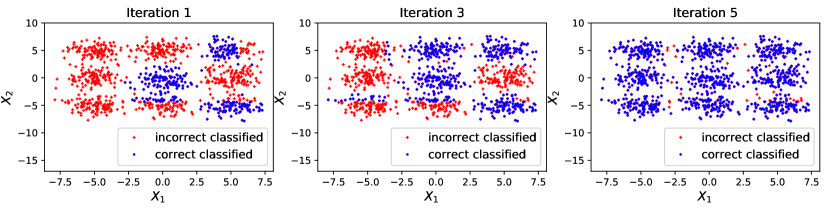
Figure 1: Demonstration on how ASCII works using the Blob data, where each learner holds one feature. The model used by each agent is a decision tree. The blue dots indicate correctly classified points, while red ones are incorrect. In this example, an agent cannot well discriminate all classes on its own, but ASCII helps it to achieve desirable performance.

III-C More discussions

In this subsection, we include more discussions on the stop criterion, complexity analysis, and interpretations through some special cases.

Stop criteria. The stop criterion as an input of Algorithm 1 guides A when to stop the assisted classification with B. We suggest two stop criteria for practice use. With the first stop criterion, the procedure of iterative assistance is repeated $K$ times until $\bar{r}_{t}^{({\texttt{A}})}\leq 1/K.$ It can be verified that this condition is equivalent to $\alpha_{t}^{({\texttt{A}})}\leq 0$. An insight of the stopping criteria is that when the current local model is worse than random guessing, the algorithm should be terminated. Our experiments and uploaded codes are based on this criterion.

The second stop criterion we suggest is to use the cross-validation technique [25, 26]. In particular, A and B only use a part of the data (e.g. the first 50% rows aligned by data IDs) to perform the assisted learning. They preserve the remaining rows to evaluate A’s performance as if in the prediction stage. The learning process continues until A’s average out-sample predictive error no longer decreases. The cross-validation is a general method with theoretical guarantees on the generalization capability  [27]. Nevertheless, the produced predictive performance has been practically and theoretically shown to be sensitive to the training-testing splitting ratio [27]. Also, A may not be able to do a re-training after the validation procedure due to communication/computation constraints. Due to the above concerns, we used the other criterion in the experiments.

Algorithm complexity. In each iteration of Algorithm 1, A and B each trains a model. This part of complexity depends on the specific models used by A and B. Additionally, A and B each calculates the ignorance score with computational and storage complexity $O(n)$ (where $n$ is the sample size). As a result, the overall complexity for A is $O(nI+c_{\texttt{A}}I)$, where $c_{\texttt{A}}$ is her own model complexity and $I$ is the number of iterations. Similar complexity applies to B.

Interpretation of the derived $\alpha_{t}^{({\texttt{A}})}$ and $\mathbf{w}_{t}^{({\texttt{A}})}$. The derivation of $\mathbf{w}_{t}^{({\texttt{A}})}$ indicates that the samples not well-modeled by A will be relatively more focused by B. Similar arguments apply to $\mathbf{w}_{t}^{({\texttt{B}})}$. We define $n_{{\texttt{A}}}=\sum_{i=1}^{n}w_{t,i}^{({\texttt{A}})}r_{t,i}^{({\texttt{A}})}$ and $n_{\bar{\texttt{A}}}=\sum_{i=1}^{n}w_{t,i}^{({\texttt{A}})}(1-r_{t,i}^{({\texttt{A}})})$. At iteration $t$, the value of $\alpha_{t}^{({\texttt{A}})}$ can be represented as

$$\alpha_{t}^{({\texttt{A}})}\approx\log(K-1)+\log\biggl{(}\frac{n_{{\texttt{A}}}}{n_{\bar{\texttt{A}}}}\biggr{)},$$

which implies that less important samples are mis-classified, a larger model weight will be given. If all the samples are correctly classified by the current model, $\alpha_{t}^{({\texttt{A}})}$ becomes infinity. The value of $\alpha_{t}^{({\texttt{B}})}$ is related to both $\alpha_{t}^{({\texttt{A}})}$ and B’s own predictive performance. In particular, when $\alpha_{t}^{({\texttt{A}})}$ is close to zero, $\alpha_{t}^{({\texttt{B}})}$ will be close to

$$\alpha_{t}^{({\texttt{B}})} \approx\log(K-1)+\log\biggl{(}\frac{n_{\bar{\texttt{A}},B}+n_{{\texttt{A}},{\texttt{B}}}}{n_{\bar{\texttt{A}},\bar{B}}+n_{{\texttt{A}},\bar{\texttt{B}}}}\biggr{)}$$

$$=\log(K-1)+\log\biggl{(}\frac{n_{{\texttt{B}}}}{n_{\bar{\texttt{B}}}}\biggr{)}.$$

Objective privacy. While in our algorithm, each agent needs to access the original task label, it does not necessarily leak the task initiator’s private learning objective. More specifically, to receive assistance from others, A only needs to send the numerical task label, and the semantic information of A’s underlying task is not shared. In this case, ASCII can improve A’s predictive performance while maintaining a private objective.

A toy example for interpretations. We illustrate how our algorithm works on a nine-class ‘Blobs’ data, and snapshot the fitted results in Figure 1 to illustrate how the algorithm alternates between two agents ${\texttt{A}},{\texttt{B}}$ in order to perform A’s learning performance.

IV Extension to Multi-Agent Scenarios

We now briefly explain the extension of Algorithm 1 to multi-agent scenarios where the objective is given in (8). In addition to the notation introduced in Section II-A, we suppose that the ignorance score is exchanged in a chain of agents, say $1\to 2\ldots\to M$, and the last agent will transmit the score to the first agent, who will then initialize a new round of interactions (demonstrated in Figure 2). We will perform empirical studies to compare the performance from a deterministic chain with a random sequence of agents (with replacement). An adaptive selection of the order of interchange is left as future work.

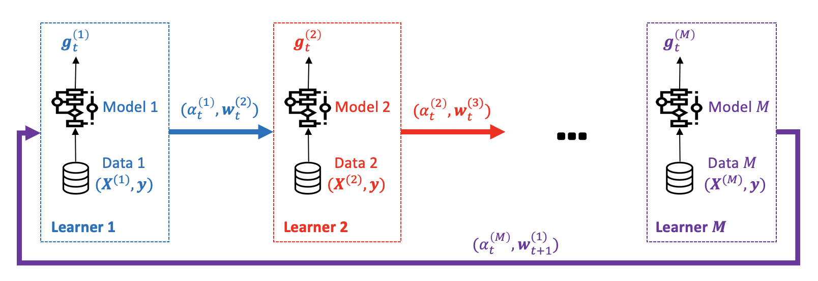
Figure 2: Demonstration of the algorithmic update in the presence of $M$ agents.

Suppose $M$ agents access the label matrix $\mathbf{Y}=[\mathbf{y}_{1},\mathbf{y}_{2},\ldots,\mathbf{y}_{n}]$, and each agent $m$ possesses a feature matrix $\mathbf{X}^{(m)}=[\mathbf{x}_{1}^{(m)},\ldots,\mathbf{x}_{n}^{(m)}]^{\mathrm{\scriptscriptstyle T}}$, a model class $\mathcal{F}_{0}^{(m)}$ and a loss function $\ell^{(m)}$ for $m=1,2,\ldots,M$. At iteration $t$, for agent $m$, under the forward stage-wise additive modeling scheme, denote the already-learned virtually-joint model from previous $t-1$ iterations as

$$\mathbf{g}_{0:t-1}(\mathbf{x}_{i}^{(1)},\mathbf{x}_{i}^{(2)},\ldots,\mathbf{x}_{i}^{(M)})=\sum_{\tau=1}^{t-1}\sum_{j=1}^{M}\alpha^{(j)}_{\tau}\mathbf{g}^{(j)}_{\tau}(\mathbf{x}_{i}^{(j)}),$$

where we initialize $\mathbf{g}_{0:0}:(\mathbf{x}^{(1)},\ldots,\mathbf{x}^{(M)})\mapsto\mathbf{0}$. Similar as (8), the optimization function can be expressed as

$$\min_{\alpha_{t}^{(m)}}\sum_{i=1}^{n}\ell\biggl{(}\mathbf{y}_{i},\mathbf{g}_{0:t-1}(\mathbf{x}_{i}^{(1)},\ldots,\mathbf{x}_{i}^{(M)})+\sum_{j=1}^{m}\alpha^{(j)}_{t}\mathbf{g}^{(j)}_{t}(\mathbf{x}_{i}^{(j)})\biggr{)}.$$

Under the forward stage-wise additive modeling scheme, at iteration $t$, agent $m$ receives the ignorance score $\mathbf{w}_{t}^{(m)}$ from agent $m-1$ (or from agent $M$ at iteration $t-1$ if $m=1$), and minimizes the exponential in-sample prediction loss that considers the additive models until $\mathbf{g}_{t}^{(m)}$. The objective function for the agent $m$ is

$$\min_{\alpha^{(m)}_{t}\in\mathbb{R},\,\mathbf{g}^{(m)}_{t}\in\mathcal{F}^{(m)}_{0}}\sum_{i=1}^{n}w_{t,i}^{(m)}e^{-\frac{1}{K}\mathbf{y}_{i}^{\mathrm{\scriptscriptstyle T}}\bigl{\{}\sum_{j=1}^{m}\alpha^{(j)}_{t}\mathbf{g}_{t}^{(j)}(\mathbf{x}^{(j)}_{i})\bigr{\}}},$$

where $\mathbf{w}_{t}^{(m)}=[w_{t,1}^{(m)},w_{t,2}^{(m)},\ldots,w_{t,n}^{(m)}]^{\mathrm{\scriptscriptstyle T}}$ , and $\alpha^{(j)}_{t},\,j=1,2,\ldots,m-1$ that have been transferred by $m-1$ preceding agents are known parameters. (13) is the specific case when $M=2$. Similarly, $\mathbf{g}_{t}^{(m)}$ is learned from the objective function

$$\min_{\mathbf{g}_{t}^{(m)}\in\mathcal{F}_{0}^{(m)}}\sum_{i=1}^{n}w_{t,i}^{(m)}\exp\{-\frac{1}{K}\alpha_{t}^{(m)}\mathbf{y}_{i}^{\mathrm{\scriptscriptstyle T}}\mathbf{g}_{t}^{(m)}(\mathbf{x}_{i}^{(m)})\},$$

and can be solved according to Proposition 1, which is the output of $\text{WST}(\mathbf{Y},\mathbf{X}^{(m)},\mathbf{w}_{t}^{(m)},\ell^{(m)},\mathcal{F}^{(m)}_{0})$.

Consider the agent $m$ at iteration $t$, the side information from previous iterations are already reflected in $\mathbf{w}_{t}^{(m)}$, The above objective function can be rewritten as

$$\min_{\alpha_{t}^{(m)},g_{t}^{(m)}}\biggl{\{} \sum_{I_{t}^{(m)}}w_{t,i}^{(m)}e^{-\frac{1}{K}\mathbf{y}_{i}^{\mathrm{\scriptscriptstyle T}}\{\sum_{j=1}^{m-1}\alpha^{(j)}_{t}\mathbf{g}_{t}^{(j)}(\mathbf{x}^{(j)}_{i})\}}e^{-\frac{1}{K-1}\alpha_{t}^{(m)}}$$

$$+\sum_{I_{\bar{t}}^{(m)}}w_{t,i}^{(m)}e^{-\frac{1}{K}\mathbf{y}_{i}^{\mathrm{\scriptscriptstyle T}}\{\sum_{j=1}^{m-1}\alpha^{(j)}_{t}\mathbf{g}_{t}^{(j)}(\mathbf{x}^{(j)}_{i})\}}e^{\frac{1}{(K-1)^{2}}\alpha_{t}^{(m)}}\biggr{\}},$$

where $\mathbf{g}_{t}^{(m)}$ is implicitly defined in $I_{t}^{(m)}$ and $I_{\bar{t}}^{(m)}$, where $I_{t}^{(m)}=\bigl{\{}i:\mathbf{g}_{t}^{(m)}(\mathbf{x}_{i}^{(m)})=\mathbf{y}_{i}\bigr{\}}$ and $I_{\bar{t}}^{(m)}=\bigl{\{}i:\mathbf{g}_{t}^{(m)}(\mathbf{x}_{i}^{(m)})\neq\mathbf{y}_{i}\bigr{\}}$.

It can be verified that the above function is convex in $\alpha_{t}^{(m)}$. Taking the derivative with respect to $\alpha_{t}^{(m)}$, and letting it be zero, we obtain the optimum at

$$\alpha_{t}^{(m)} =\biggl{\{}\log\frac{\sum_{I_{t}}w_{t,i}^{(m)}e^{-\frac{1}{K}\mathbf{y}_{i}\bigl{\{}\sum_{j=1}^{m-1}\alpha^{(j)}_{t}\mathbf{g}_{t}^{(j)}(\mathbf{x}^{(j)}_{i})\bigr{\}}}}{\sum_{I_{\bar{t}}}w_{t,i}^{(m)}e^{-\frac{1}{K}\mathbf{y}_{i}\bigl{\{}\sum_{j=1}^{m-1}\alpha^{(j)}_{t}\mathbf{g}_{t}^{(j)}(\mathbf{x}^{(j)}_{i})\bigr{\}}}}$$ (18)

$$\quad+\log(K-1)\biggr{\}}\times\frac{K}{(K-1)^{2}}.$$

Since $K/(K-1)^{2}$ is a constant for all $\alpha_{t}^{(m)},\,t=1,2,\ldots,\,m=1,2,\ldots,M$, it can be removed from (18) without changing the algorithmic output. From (18), $\alpha_{t}^{(m)}$ will be larger if more important samples (with larger $w_{t,i}^{(m)}$) are correctly classified by $\mathbf{g}_{t}^{(m)}$. We then update the ignorance score. Figure 2 describes how each agent interchanges with each other. If $m\neq M$, the ignorance that agent $m$ transmits to $m+1$ is

$$w_{t,i}^{(m+1)}=\frac{w_{t,i}^{(m)}\times\exp\{\alpha_{t}^{(m)}(1-r_{t,i}^{(m)})\}}{\sum_{i=1}^{n}w_{t,i}^{(m)}\times\exp\{\alpha_{t}^{(m)}(1-r_{t,i}^{(m)})\}}$$

for $m>0$. If $M=1$, the new ignorance score will be transmitted to agent $1$ at next round of iteration, which is

$$w_{t+1,i}^{(1)}=\frac{w_{t,i}^{(M)}\times\exp\{\alpha_{t}^{(M)}(1-r_{t,i}^{(M)})\}}{\sum_{i=1}^{n}w_{t,i}^{(M)}\times\exp\{\alpha_{t}^{(M)}(1-r_{t,i}^{(M)})\}}.$$

The interchanges at different iterations are therefore connected between agent $M$ and agent $1$.

V Other Variants

In this section, we also consider some variants of the ASCII method developed in previous sections, which also aim to solve (8). They will be experimentally compared in Section VI.

Method 1 (ASCII-Simple). The first method is similar to ASCII when transferring ignorance scores as described in Equations (15) and (17), and the only difference is that the update of $\alpha_{t}^{(m)}$ is based on $m$th agent’s individual exponential loss (in the line 8 of Algorithm 1). Take the two-agent Algorithm 1 as an example. The pseudocode for ASCII-Simple is briefly summarized below.

• A learns $\mathbf{g}_{t}^{({\texttt{A}})}$ and $\alpha_{t}^{({\texttt{A}})}$ based on the optimization function (12).

• A calculates the ignorance score $\mathbf{w}_{t}^{({\texttt{B}})}$ as in (15) and passes it to B.

• B learns $\mathbf{g}_{t}^{({\texttt{B}})}$ and $\alpha_{t}^{({\texttt{B}})}$ on the optimization function $\min_{\alpha_{t}^{({\texttt{B}})}}\sum_{i=1}^{n}w_{t,i}^{({\texttt{B}})}\exp\{-\frac{1}{K}\mathbf{y}_{i}^{{\mathrm{\scriptscriptstyle T}}}\alpha^{({\texttt{B}})}_{t}\mathbf{g}^{({\texttt{B}})}_{t}(\mathbf{x}_{i}^{({\texttt{B}})})\}$.

• B calculates the ignorance score as in (17) and passes to A at the next round of iteration.

Intuitively, this method may not be as efficient as the ASCII as the side information of model-level performance was not transmitted to accelerate the learning efficiency. It is conceivable that ASCII will perform better when finish same round of iterations, which is observed our experimental results VI-C.

Method 2 (ASCII-Random). The second method is to randomly shuffle the order of interchange at each iteration. In other words, the ASCII-Random uses the order of $\pi_{t}(1),\ldots,\pi_{t}(M)$ where $\pi_{t}$ denotes a random permutation at each iteration $t$.

Method 3 (Ensemble-Adaboost). The third method is that we ignore the interchange between agents, so that each agent learns an Adaboost model and the final prediction uses a majority vote of all the agents.

VI Experimental Study

We provide numerical demonstrations of the proposed method. For the synthetic data, we replicated 20 times for each method. In each replication, we trained on a dataset with size $10^{3}$, and then tested on a dataset with size $10^{5}$. We chose a testing size much larger than the training size to produce a fair comparison of out-sample predictive performance [28]. For the real data, we trained on 70% and tested on 30% of data, re-sampled with replacement 20 times to average the performance and to evaluate standard errors. The ‘oracle score’ is the testing error obtained by the model that is trained on the pulled data.

VI-A ASCII for improving accuracy to near-oracle

We test on synthetic and real data to verify that the proposed method can significantly improve the classification performance for a single agent. The real data considered are listed below.

$\bullet$MIMIC3 Data. Medical Information Mart for Intensive Care III [29] (MIMIC3) is a comprehensive clinical database that contains de-identified information for 38,597 distinct adult patients admitted to critical care units between 2001 and 2012 at a Medical Center. We focus on the task of predicting if a patient would have an extended Length of Stay ($>$ 7 days) based on the first 24 hours information. Following the processing procedures in [30, 31], we select 16 medical features and 15000 patients. We partition the data into two agents according to the original data sources, with one holding three features and the other holding 12 features.

$\bullet$ QSAR biodegradation Data. The quantitative structure-activity relationship (QSAR) biodegradation dataset was built in the Milano Chemometrics and QSAR Research Group [32]. The whole dataset has 41 attributes and 2-class labels, with 1055 data in total. We partition the data vertically into two parts for two agents who hold 20 and 21 features.

$\bullet$ Red Wine Quality Data. The red wine classification dataset has 1600 data, 11 attributes, and 6-class labels [33]. We partition the data into two agents, the first holding six features, and the second one holding five features.

$\bullet$ Blob Data (Synthetic). We generate isotropic Gaussian blobs for clustering. $\mathbf{X}\in\mathbb{R}^{1000\times 8}$ is the feature matrix and $\mathbf{c}\in\mathbb{R}^{1000}$ is the 10-class label. Suppose that there exist four agents, and each holds two non-overlapping columns in $\mathbf{X}$. For simplicity, we let each agent use a random forest model with the same number of trees and depth.

We suppose that each agent uses a decision tree classifier for the above data except for the blob data. The results summarized in Figure 3 indicate that our proposed method performs significantly better than that of a single agent and often nearly oracle within a few rounds of assistance.

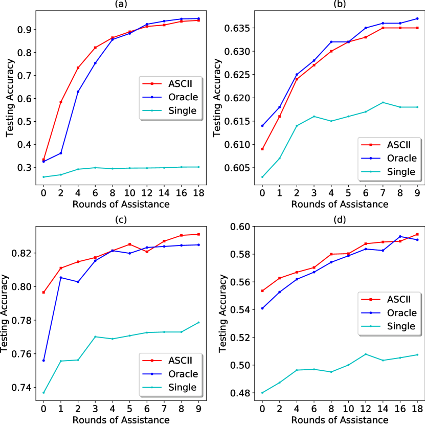
Figure 3: Out-sample predictive accuracy of the proposed method (‘ASCII’), the oracle method unrealistically using the pulled data (‘Oracle’), and the non-assisted method using only agent A’s data (‘Single’), against the number of rounds for the datasets of (a) Blob, (b) MIMIC, (c) QSAR, and (d) Wine, as described in the text. The model used by each agent (a) is random forest, and decision tree in (b)(c)(d). Standard errors over 20 independent replications are within 0.04.

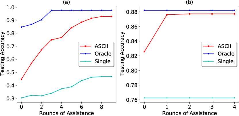
Figure 4: Out-sample predictive accuracy for the datasets of (a) Gaussian Blob data (b) Fashion-MNIST, where the transmission costs are improved by around 10 and 195 times respectively, when compared to the oracle approach. The costs are evaluated using the number of bits needed for transmission at $90\%$-oracle test accuracy. The methods used on blob and Fashion-MNIST data are random forest and 3-layer neural network, respectively.

VI-B ASCII for reducing transmission cost

We use two examples to illustrate that ASCII can significantly reduce the transmission cost while maintaining near-oracle performance. Compared with transmitting raw data from B to A, ASCII only requires transmitting ignorance score (length $n$) and model weight (scalar) at each round of iteration. We use our algorithm to show that ASCII can approximate the oracle, with much less transmission costs when compared with transmitting data from agent B to A.

The first is Gaussian Blob data, which is generated from 5 features and 10 classes. Additionally, 195 redundant features are generated and appended to the above 5 features. We randomly divide these 200 features into 2 agents, each agent holding 100 features. Each agent performs a random forest classifier with the same depth and number of trees. The result is shown in Figure 4.

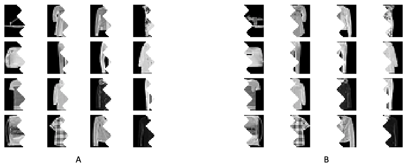
Figure 5: An example pictures in A and B, A holds half of the picture and B holds another half.

The second example utilizes Fashion-MNIST, an accessible classification dataset with 10 classes in total, each sample being a $28\times 28$ matrix with entries $0$-$255$. It has $6\cdot 10^{4}$ training and $10^{4}$ testing samples, respectively. Suppose that agent A and B both hold half part of each image, as illustrated in Figure 5. B does not want to share the picture with A (possibly due to privacy and transmission costs). Thus, each agent possesses partial information of the same objects. We used 3-layer neural networks to build the model, and summarize the results in Figure 4. Though neural networks are expressive, a single learner’s predictive performance is still restricted because of limited information. The plot shows that after only two iterations, the testing performance is close to the oracle. As a result, the transmission cost of ASCII compared with the oracle (passing B’s data to A) is reduced over 100 times in terms of the number of transmitted bits.

The result summarized in Figure 4 shows that the transmission cost of ASCII compared with the oracle (passing B’s data to A) is reduced over 100 times in terms of the number of transmitted bits.

VI-C ASCII compared with other methods

In this subsection, we illustrate that ASCII can outperform the variants mentioned in Section V.

Blob Data (Synthetic). We generate $20$-class isotropic Gaussian blobs for clustering. For training data, the centralized feature matrix $\mathbf{X}\in\mathbb{R}^{1000\times 20}$ is held by $20$ agents, each holding $1$ heterogeneous feature. Let $\mathbf{c}\in\mathbb{R}^{1000}$ be the $20$-class label. Suppose that each agent uses logistic regression for classification. The result is shown in Figure 6.

Red wine quality data. The red wine classification data set has 1600 data, 11 attributes, and 6 class labels. Suppose that each agent holds a unique feature, and uses a decision tree classifier.

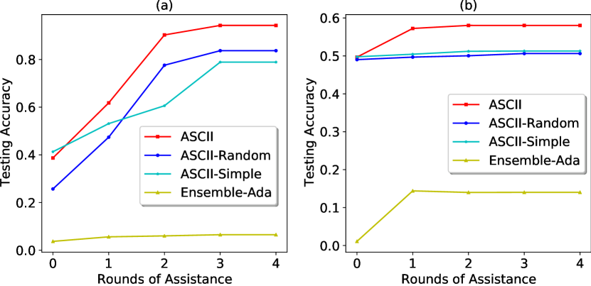
Figure 6: Out-sample predictive accuracy of the proposed method (‘ASCII’), the ASCII method in a random assistance manner (‘ASCII-Random’), the ASCII method that only transfer ignorance score (‘ASCII-Simple’) and the non-assistance Ensemble Adaboost (‘Ensemble-Ada’) against the number of rounds for the datasets of (a) Blob, (b) Wine, as described in the text. The model used by each agent in (1)and (2) are logistic regression and decision tree. Standard errors over 20 independent replications are within 0.04.

The result indicates that ASCII can outperform other related methods since ASCII-Simple only considers the interchange of data-level side information. ASCII-Random performs similar or slightly better than ASCII-Simple, but still not as good as ASCII, the possible reason is that ASCII-Random takes the model-level side information interchange into account, but ASCII-Random may result some extreme cases, such as A may still interchange with A at the end of one iteration and the begin of next iteration. This may lose some power of interchanging information, because A usually can’t provide more information other than models. Ensemble Adaboost is the worst since it neither considers model-level or data-level side information, there exists no assistance between agents. The results are aligned with our explanations in Section V, and it turns out that the transmission of model weight and the ignorance score are both necessary since agents provide their supplement information on samples and models to agent $1$.

VII Conclusion

In this paper, we proposed a general method for an agent to improve its classification performance by iteratively interchanging ignorance scores with other agents. Our method is naturally suitable for autonomous learning scenarios where private raw data cannot be shared. Moreover, the proposed method allows agents to use private local models or algorithms, which is appealing in many application domains.

Some future directions are summarized as follows. First, our work addressed classification, and we believe that similar techniques can be emulated to study regression problems. Second, from various experiments, we observed that a single agent often achieves near-oracle performance by interchanging with other agents in random orders. This motivates the problem to study the most efficient order of interchanging information to attain the optimum. Another open problem is to study how asynchronous interchange, meaning different orders at two rounds, will influence the learning efficiency.

References

• [1] X. Xian, X. Wang, J. Ding, and R. Ghanadan, “Assisted learning: A framework for multiple organizations’ learning,” 2020.
• [2] A. C. Yao, “Protocols for secure computations,” in Proc. SFCS.   IEEE, 1982, pp. 160–164.
• [3] D. Chaum, C. Crépeau, and I. Damgard, “Multiparty unconditionally secure protocols,” in Proc. STOC, 1988, pp. 11–19.
• [4] C. Dwork and K. Nissim, “Privacy-preserving datamining on vertically partitioned databases,” in Proc. CRYPTO.   Springer, 2004, pp. 528–544.
• [5] C. Gentry, “Fully homomorphic encryption using ideal lattices,” in Proc. STOC, 2009, pp. 169–178.
• [6] C. Dwork, “Differential privacy,” Encyclopedia of Cryptography and Security, pp. 338–340, 2011.
• [7] F. Armknecht, C. Boyd, C. Carr, K. Gjøsteen, A. Jäschke, C. A. Reuter, and M. Strand, “A guide to fully homomorphic encryption,” Cryptology ePrint Archive, p. 1192, 2015.
• [8] M. Stojanovic and J. Preisig, “Underwater acoustic communication channels: Propagation models and statistical characterization,” IEEE Commun. Mag., vol. 47, no. 1, pp. 84–89, 2009.
• [9] R. Schettini and S. Corchs, “Underwater image processing: state of the art of restoration and image enhancement methods,” EURASIP J. Adv. Signal Process., vol. 2010, p. 14, 2010.
• [10] E. Diao, J. Ding, and V. Tarokh, “Drasic: Distributed recurrent autoencoder for scalable image compression,” Proc. DSC, 2019.
• [11] ——, “Multimodal controller for generative models,” arxiv preprint arxiv:2002.02572, 2020.
• [12] D. Lahat, T. Adali, and C. Jutten, “Multimodal data fusion: an overview of methods, challenges, and prospects,” Proc. IEEE, vol. 103, no. 9, pp. 1449–1477, 2015.
• [13] R. Shokri and V. Shmatikov, “Privacy-preserving deep learning,” in Proc. SIGSAC, 2015, pp. 1310–1321.
• [14] J. Konecny, H. B. McMahan, F. X. Yu, P. Richtarik, A. T. Suresh, and D. Bacon, “Federated learning: Strategies for improving communication efficiency,” arXiv preprint arXiv:1610.05492, 2016.
• [15] H. B. McMahan, E. Moore, D. Ramage, S. Hampson et al., “Communication-efficient learning of deep networks from decentralized data,” arXiv preprint arXiv:1602.05629, 2016.
• [16] K. Cheng, T. Fan, Y. Jin, Y. Liu, T. Chen, and Q. Yang, “Secureboost: A lossless federated learning framework,” arXiv preprint arXiv:1901.08755, 2019.
• [17] Z. Fengy, H. Xiong, C. Song, S. Yang, B. Zhao, L. Wang, Z. Chen, S. Yang, L. Liu, and J. Huan, “Securegbm: Secure multi-party gradient boosting,” arXiv preprint arXiv:1911.11997, 2019.
• [18] Q. Yang, Y. Liu, T. Chen, and Y. Tong, “Federated machine learning: Concept and applications,” in Proc. TIST, vol. 10, no. 2, pp. 1–19, 2019.
• [19] Y. Liu, Y. Kang, X. Zhang, L. Li, Y. Cheng, T. Chen, M. Hong, and Q. Yang, “A communication efficient vertical federated learning framework,” arXiv preprint arXiv:1912.11187, 2019.
• [20] Y. Freund and R. E. Schapire, “A desicion-theoretic generalization of on-line learning and an application to boosting,” in Proc. EuroCOLT.   Springer, 1995, pp. 23–37.
• [21] D. D. Margineantu and T. G. Dietterich, “Pruning adaptive boosting,” in ICML, vol. 97.   Citeseer, 1997, pp. 211–218.
• [22] J. Friedman, T. Hastie, R. Tibshirani et al., “Additive logistic regression: a statistical view of boosting,” Ann. Stat., vol. 28, no. 2, pp. 337–407, 2000.
• [23] T. Hastie, S. Rosset, J. Zhu, and H. Zou, “Multi-class adaboost,” Statistics and its Interface, vol. 2, no. 3, pp. 349–360, 2009.
• [24] Y. Lee, Y. Lin, and G. Wahba, “Multicategory support vector machines: Theory and application to the classification of microarray data and satellite radiance data,” J. Am. Stat. Assoc., vol. 99, no. 465, pp. 67–81, 2004.
• [25] D. M. Allen, “The relationship between variable selection and data agumentation and a method for prediction,” Technometrics, vol. 16, no. 1, pp. 125–127, 1974.
• [26] S. Geisser, “The predictive sample reuse method with applications,” J. Amer. Statist. Assoc., vol. 70, no. 350, pp. 320–328, 1975.
• [27] J. Ding, V. Tarokh, and Y. Yang, “Model selection techniques: An overview,” IEEE Signal Process. Mag., vol. 35, no. 6, pp. 16–34, 2018.
• [28] ——, “Model selection techniques: An overview,” IEEE SignaProcess. Mag., vol. 35, no. 6, pp. 16–34, 2018.
• [29] A. E. Johnson, T. J. Pollard, L. Shen, H. L. Li-wei, M. Feng, M. Ghassemi, B. Moody, P. Szolovits, L. A. Celi, and R. G. Mark, “Mimic-iii, a freely accessible critical care database,” Sci. Data, vol. 3, p. 160035, 2016.
• [30] H. Harutyunyan, H. Khachatrian, D. C. Kale, G. V. Steeg, and A. Galstyan, “Multitask learning and benchmarking with clinical time series data,” arXiv preprint arXiv:1703.07771, 2017.
• [31] S. Purushotham, C. Meng, Z. Che, and Y. Liu, “Benchmarking deep learning models on large healthcare datasets,” J. Biomed. Inform, vol. 83, pp. 112–134, 2018.
• [32] K. Mansouri, T. Ringsted, D. Ballabio, R. Todeschini, and V. Consonni, “Quantitative structure–activity relationship models for ready biodegradability of chemicals,” J. Chem. Inf. Model., vol. 53, no. 4, pp. 867–878, 2013.
• [33] P. Cortez, A. Cerdeira, F. Almeida, T. Matos, and J. Reis, “Modeling wine preferences by data mining from physicochemical properties,” Decis. Support Syst., vol. 47, no. 4, pp. 547–553, 2009.