Continuous-variable graph states for quantum metrology

Abstract

Graph states are a unique resource for quantum information processing, such as measurement-based quantum computation. Here, we theoretically investigate using continuous-variable graph states for single-parameter quantum metrology, including both phase and displacement sensing. We identified the optimal graph states for the two sensing modalities and showed that Heisenberg scaling of the accuracy for both phase and displacement sensing can be achieved with local homodyne measurements.

I Introduction

Quantum metrology is among the most important applications of quantum information science, which aims at using quantum mechanical techniques and resources, such as noise squeezing and entanglement, to enhance the accuracy of parameter estimation beyond any classical means giovannetti2004quantum ; giovannetti2006quantum ; degen2017quantum ; pirandola2018advances . One pronounced example is the use of squeezed light in interferometric gravitational wave detectors to probe weak mechanical displacement beyond the standard quantum limit abadie2011gravitational ; aasi2013enhanced .

Besides quantum sensing using a single electromagnetic mode, which typically exploits the quantum correlation between its two quadratures, multi-mode quantum metrology that is relevant to distributed sensing uses non-classical inter-modal correlations to achieve advantages over classical resources, such as realization of the Heisenberg limit of the sensitivity in terms of, for example, the total number of modes. Multi-mode metrology based on both discrete variables holland1993interferometric ; mitchell2004super ; humphreys2013quantum and continuous variables (CV) anisimov2010quantum ; zhuang2018distributed ; matsubara2019optimal ; guo2020distributed has gained discussions in the literature. For the latter, many considered scenarios though rely on the output of highly squeezed states intertwined via a network of beam splitters as the probe.

Here, we consider another type of entangled states–graph states–as the probe for distributed quantum metrology. Graph states are deemed as a unique resource for measurement-based quantum computing. Recently, discrete-variable graph states have also drawn attention for applications in quantum sensing rosenkranz2009parameter ; friis2017flexible ; shettell2020graph . In this paper, we study for the first time CV graph states for quantum metrology, including both phase and displacement sensing, of a single unknown parameter. We calculated the quantum Fisher information (QFI) for both cases with arbitrary graph states and identified the graph states to achieve the optimal scaling of sensitivity. Furthermore, we show that the QFI of both phase and displacement sensing can be attained (up to an $O(1)$ factor) using local homodyne measurements, highlighting the practicality of this scheme.

The general scenario of quantum metrology deploying CV graph states is schematically illustrated in Fig. 1. The CV graph state with density matrix $\hat{\rho}$ is generated using the canonical method by applying $C_{z}$ gates onto a cluster of squeezed vacuum states $\ket{0,r}$, where $r$ is the squeeze factor. In this way, the graph state can be represented by a graph, where each vertex corresponds to a squeezed vacuum and an edge connecting two vertices represents the applied $C_{z}$ gate. The CV graph state then experiences a unitary transformation $\hat{U}_{\phi}$ which encodes the unknown variable $\phi$ onto the graph state, i.e., $\hat{\rho}_{\phi}=\hat{U}_{\phi}\hat{\rho}\hat{U}_{\phi}^{\dagger}$. Finally, proper measurements described by positive-operator valued measures (POVMs) $\mathcal{P}$ are performed on the transformed state $\hat{\rho}_{\phi}$ to extract the information about $\phi$.

The accuracy of measuring $\phi$ is subject to measurement and fundamental noises. It is known that, for a given set of POVMs, the sensitivity $\delta\phi$ is constrained by the classical Cramer-Rao bound whose lower limit is given by the quantum Cramer-Rao bound–a quantity that is intrinsic to the probe state and the parameter-encoding transformation yet independent of POVMs, i.e.,

$$\delta\phi\geq 1/\sqrt{I(\phi|\mathcal{P},\hat{\rho})}\geq 1/\sqrt{F(\phi|\hat{\rho})},$$ (1)

where $I(\phi|\mathcal{P},\hat{\rho})$ and $F(\phi|\hat{\rho})$ are the Fisher information (FI) associated with the POVM $\mathcal{P}$ and the QFI, respectively paris2009quantum ; toth2014quantum . In principle, for single-parameter metrology, POVMs can always be constructed such that the corresponding FI saturates the fundamental QFI paris2009quantum . With proper quantum states as the probe, the quantum Cramer-Rao bound may achieve the Heisenberg scaling in terms of relevant resources, i.e., $\delta\phi\propto 1/n$, where $n$ could be, for example, the total number of photons or the number of modes. While with classical probe states, the best available sensitivity always complies with the standard quantum limit, i.e., $\delta\phi\propto 1/\sqrt{n}$.

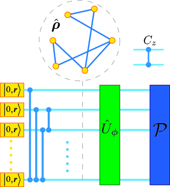
Figure 1: Schematic plot illustrating generation of the CV graph state by applying $C_{z}$ gates onto squeezed vacuum states and its use in quantum metrology.

Given $n$ bosonic modes with annihilation and creation operators $\{\hat{a}_{k},\hat{a}_{k}^{\dagger}\}$, or equivalently quadrature operators $\hat{q}_{k}=(\hat{a}_{k}+\hat{a}_{k}^{\dagger})/\sqrt{2}$, $\hat{p}_{k}=(\hat{a}_{k}-\hat{a}_{k}^{\dagger})/(i\sqrt{2})$, $k=1,...,n$, CV states created from these modes are typically described by the Wigner function of a Gaussian form

$$W(\mathbf{x})=\frac{\exp\left[-\frac{1}{2}(\mathbf{x}-\overline{\mathbf{x}})^{T}\mathbf{\Sigma}^{-1}(\mathbf{x}-\overline{\mathbf{x}})\right]}{(2\pi)^{n}\sqrt{\operatorname{det}\mathbf{\Sigma}}},$$ (2)

where $\hat{\mathbf{x}}:=\left(\hat{q}_{1},\hat{p}_{1},\ldots,\hat{q}_{n},\hat{p}_{n}\right)^{T}$, $\overline{x}_{i}=\Tr(\hat{x}_{i}\hat{\rho})$ , and $\Sigma_{ij}:=\frac{1}{2}\left\langle\left\{\hat{x}_{i}-\left\langle\hat{x}_{i}\right\rangle,\hat{x}_{j}-\left\langle\hat{x}_{j}\right\rangle\right\}\right\rangle$ is the covariance matrix ($\{~{},~{}\}$ is the anti-commutator) weedbrook2012gaussian . Our calculation uses the formulation of CV graph states generated from the finite squeezed vacuum simon1988gaussian ; menicucci2011graphical . Such CV graph states possess a covariance matrix

$$\Sigma=\frac{1}{2}SS^{T},$$ (3)

where $S$ is a symplectic matrix, and it can be further decomposed into the following form,

$$\Sigma=\frac{1}{2}\left[\begin{matrix}U^{-1}&U^{-1}V\\ VU^{-1}&U+VU^{-1}V\end{matrix}\right],$$ (4)

where $U$ is symmetric and positive definite and $V$ is symmetric. For graph states created by the canonical method with $\hat{C}_{z}=\exp\left[\frac{i}{2}\hat{q}_{1}\otimes\hat{q}_{2}\right]$, where $\hat{q}_{1}$ and $\hat{q}_{2}$ are the position operators of the two involved modes, we have menicucci2011graphical

$$U=e^{-2r}I,\quad V=A,$$ (5)

where $r$ is the squeeze parameter of the input squeezed vacuum $\ket{0,r}\equiv\exp[\frac{r}{2}a^{2}-\frac{r}{2}a^{\dagger 2}]\ket{0}$, $I$ is the identity matrix and $A$ is the adjacency matrix of the underlying graph.

II Phase sensing

II.1 QFI for phase sensing

We first consider the case of phase sensing, where the unknown parameter $\phi$ is encoded via the phase change of the probe state. The corresponding unitary transformation acting on the graph state is given by

$$\hat{U}_{\phi}=\exp(-i\sum_{j=1}^{n}\phi f_{j}\hat{a}^{\dagger}_{j}\hat{a}_{j}),$$ (6)

where $n$ is the number of modes constituting the graph state, $\hat{a}_{j}(\hat{a}^{\dagger}_{j})$ is the annihilation(creation) operator of the $j$-th mode, and $f_{j}$ is its responsivity. Eq. 6 is a passive, or energy-preserving, Gaussian unitary transformation, i.e., its generator $\hat{G}_{\phi}\equiv i\hat{U}^{\dagger}_{\phi}\frac{d\hat{U}_{\phi}}{d\phi}$ commutes with the number operator. In general, the QFI for parameter estimation using Gaussian states and passive Gaussian unitary transformations can be calculated by matsubara2019optimal

$$F(\phi|\hat{\rho})=\frac{1}{2}\Tr(G_{\phi}\Sigma^{-1}G_{\phi}\Sigma-G_{\phi}^{2}),$$ (7)

where $G_{\phi}$ is the matrix form of the generator of the Gaussian transformation.

We straightforwardly calculated the QFI for phase sensing using a CV graph state with the covariance matrix $\Sigma$ given by Eqs. 4 and 5, which yields

$$F(\phi|\hat{\rho})=2\sinh^{2}2r\sum_{j=1}^{n}f_{j}^{2}+\sum_{j,k=1}^{n}(f_{j}^{2}+e^{4r}f_{j}f_{k})A_{jk}A_{kj}+\frac{1}{2}e^{4r}\sum_{j,k=1}^{n}f_{j}f_{k}[A^{2}]_{jk}[A^{2}]_{kj},$$ (8)

where $[A^{2}]_{ij}$ is the element of matrix $A^{2}$. The first term in Eq. 8 is the QFI for $n$ independent squeezed vacuum states, and the rest terms are resulted from the entanglement generated by $C_{z}$ gates. We also calculated the total mean photon number of the CV graph state (Appendix A),

$$\mathrm{bar}{N}=n\sinh^{2}r+\frac{1}{4}e^{2r}\Tr A^{2}.$$ (9)

Similarly, the first term of Eq. 9 is the total mean photon number of $n$ uncoupled squeezed vacua and the second term is the addition due to $C_{z}$ gates.

II.2 CV graph states achieving the Heisenberg limit

In this subsection, we identify CV graph states that achieve the Heisenberg limit for phase sensing, in terms of both total number of photons and number of modes. We first consider the simplified case where $f_{j}\equiv f$, $\forall j$. The QFI given in Eq. 8 reduces to

$$F(\phi|\hat{\rho})=2nf^{2}\sinh^{2}2r+(1+e^{4r})f^{2}\Tr A^{2}+\frac{1}{2}e^{4r}f^{2}\Tr A^{4}.$$ (10)

Because we want to explore the effect of entanglement of the graph state, it is assumed that the graph is sufficiently connected and the dominant terms in Eqs. 9 and 10 are the adjacency matrix-dependent terms.

We introduce a characteristic figure that is intrinsic to the underlying graph of the CV graph state,

$$\chi_{\textrm{p}}\equiv\frac{\Tr A^{4}}{\left(\Tr A^{2}\right)^{2}}.$$ (11)

Using this characteristic figure, the QFI for a sufficiently connected graph can be expressed as

$$F(\phi|\hat{\rho})\approx 8f^{2}\chi_{\textrm{p}}\mathrm{bar}N^{2}\equiv 8f^{2}\chi_{\textrm{p}}n^{2}\widetilde{N}^{2},$$ (12)

where $\widetilde{N}=\mathrm{bar}{N}/n$ is the average number of photons per mode. It is easy to show that

$$\chi_{\textrm{p}}\leq 1$$ (13)

and the equality is asymptotically saturated when the adjacency matrix $A$ has only one largest eigenvalue (in absolute value) and the ratio between it and the other eigenvalues approaches infinity as $n$ increases. In this case, the Heisenberg limit of phase sensitivity in terms of $\mathrm{bar}N$ is achieved. When $A$ has $m>1$ largest eigenvalues, with $m$ not to scale with $n$, whose mutual ratios are asymptotically nonzero constants, the Heisenberg limit can still be achieved, yet with the QFI reduced by a factor of $O(1)$ constant comparing to the previous case.

As an example, we show that the star graph state satisfies the condition above for achieving the Heisenberg limit for phase sensing. The star graph has only one vertex adjacent to all the other vertices which are otherwise unconnected. The adjacency matrix of the star graph is given by

$$A_{ij}=\delta_{i1}+\delta_{j1}-2\delta_{i1}\delta_{j1},$$ (14)

assuming the central vertex is $j=1$, which only has two nonzero eigenvalues $\lambda_{\pm}=\pm\sqrt{n-1}$, leading to $\chi_{\textrm{p}}=\frac{1}{2}$. To be more precise, $F(\phi|\hat{\rho})\approx\frac{16}{9}f^{2}\mathrm{bar}{N}^{2}=\frac{16}{9}f^{2}n^{2}\widetilde{N}^{2}$, after taking into account of the first term of Eq. 9. Thus, the star graph state achieves the Heisenberg scaling in terms of total number of photons and the number of modes (for fixed number of photons per mode). In contrast, the separable state with $A=0$ has $F(\phi|\hat{\rho})\approx\frac{1}{2}nf^{2}e^{4r}\approx 8f^{2}\mathrm{bar}{N}^{2}/n=8f^{2}n\widetilde{N}^{2}$, which only achieves the standard quantum limit in terms of number of modes (for fixed number of photons per mode), while the Heisenberg scaling in $\mathrm{bar}N$ is weakened by a factor of $\sqrt{n}$. We plot the QFI of phase sensing (calculated using Eq. 10) for the star graph state and separable state in Fig. 2. The star graph state always outperforms the separable state. Another type of graph states that achieve the Heisenberg scaling in phase sensing is the $l-$multipartite graph states, which we detail in Appendix B.

Now we show that for the general case where $f_{j}$’s are not necessarily equal, the CV star graph state still achieves the Heisenberg limit. The QFI in this case is found to be

$$F(\phi|\hat{\rho}) \approx\frac{1}{2}e^{4r}\sum_{j=1}^{n}f_{j}^{2}+\frac{1}{2}e^{4r}\left[(n-1)^{2}f_{1}^{2}+\left(\sum_{j=2}^{n}f_{j}\right)^{2}\right]$$ (15)

$$>\frac{1}{2}e^{4r}(n-1)^{2}f_{1}^{2}$$

$$\approx\frac{8}{9}f_{1}^{2}\mathrm{bar}{N}^{2}=\frac{8}{9}f_{1}^{2}n^{2}\widetilde{N}^{2},$$

which indeed exhibits the same scaling as the equi-$f_{i}$ case. In this sense, the CV star graph state is universally optimal for phase sensing.

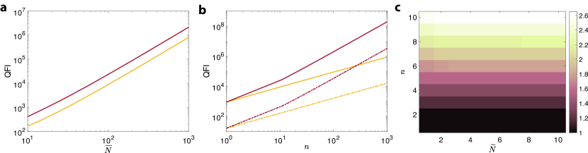
Figure 2: Comparison of QFI scaling of phase sensing between the star graph state (maroon) and separable state (yellow) with respect to (a) $\mathrm{bar}N$ for fixed $n=10$ and (b) $n$ for fixed $\widetilde{N}=1$ (dash-dotted line) and $\widetilde{N}=10$ (solid line). (c) Ratio between QFI achieved by the star graph state and separable state for small $n$ and $\widetilde{N}$. We have chosen $f=1$ in these plots.

II.3 Homodyne detection to saturate the quantum Cramer-Rao bound

While the quantum Cramer-Rao bound sets the fundamental limit of parameter estimation, an important question is whether a POVM exists whose FI saturates the QFI. Since we are only considering single-parameter estimation here, such POVM can always be found in theory paris2009quantum . However, the mathematically constructed POVM is usually difficult to implement in most cases. Here, surprisingly, we numerically find that local homodyne detection actually saturates the QFI up to an $O(1)$ factor for the phase sensing using the star graph state.

To show this, in general, the outcome of the homodyne detection (of the quadrature) of a Gaussian state is a Gaussian probability distribution regarding the unknown parameter $\phi$ adesso2014continuous ; kay1993fundamentals , which is captured by the first- and second-order moment $\omega$ and $\sigma_{M}$, respectively. The distinguishibility of probability distribution with different unknown parameter determines the sensitivity of $\phi$, which is quantified by FI. As a result, the FI can be calculated using the Gaussian probability distribution of the measurement outcome as kay1993fundamentals

$$I=\frac{1}{2}\Tr\left[\left(\frac{\partial\sigma_{M}}{\partial\phi}\sigma_{M}^{-1}\right)^{2}\right]+\left(\frac{\partial\omega}{\partial\phi}\right)^{T}\sigma_{M}^{-1}\left(\frac{\partial\omega}{\partial\phi}\right).$$ (16)

Following Refs. adesso2014continuous ; kay1993fundamentals , we find the first- and second-order moment of the homodyne detection for the phase sensing using CV graph states are given by $\omega=0$ and

$$\sigma_{M}= \frac{1}{2}\big{[}(F_{2}G_{1}-G_{2}F_{1})U^{-1}(F_{2}G_{1}-G_{2}F_{1})+(G_{1}G_{2}+F_{1}F_{2})VU^{-1}(F_{2}G_{1}-G_{2}F_{1})$$ (17)

$$+(F_{2}G_{1}-G_{2}F_{1})U^{-1}V(G_{1}G_{2}+F_{1}F_{2})+(G_{1}G_{2}+F_{1}F_{2})(U+VU^{-1}V)(G_{1}G_{2}+F_{1}F_{2})\big{]},$$

respectively, where $U$ and $V$ are given by Eq. 5, and

$$[G_{1}]_{ij}=\delta_{ij}\cos f_{j}\phi,$$ (18)

$$[F_{1}]_{ij}=\delta_{ij}\sin f_{j}\phi,$$

$$[G_{2}]_{ij}=\delta_{ij}\cos\theta_{j},$$

$$[F_{2}]_{ij}=\delta_{ij}\sin\theta_{j},$$

with $\theta_{j}$ the phase difference between the local oscillator and the $j$-th mode.

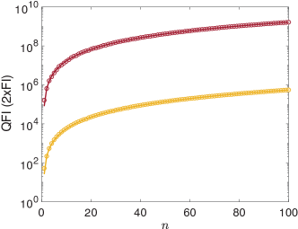
Figure 3: Numerically calculated FI of phase sensing with the star graph state and the homodyne detection with optimized local oscillator phases, for $r=1$ (yellow) and 3 (maroon). The dots are $2\times$FI. The solid line shows the analytical QFI. We have chosen $f=1$.

We numerically calculated and optimized FI, by varying $\theta_{j}$, for the star graph state with $f_{j}\equiv f$, $\forall j$. Because of the high-symmetric structure of the star graph, we expect that the maximum FI is achieved when

$$\theta_{1}=\alpha\mathrm{\ and\ }\theta_{j}=\beta,j\geq 2.$$ (19)

With this rational assumption, we find the numerically optimized FI saturates the analytical QFI given by Eq. 10 up to a constant, irrespective of $n$ (see Fig. 3 for an example).

III Displacement sensing

In this section, we consider another type of sensing modality that is displacement sensing. One canonical example of displacement sensing is found in the setting of an optomechanical cavity subject to a detuned pump, where the mechanical motion of the cavity mirror induces a displacement of the probe beam. For the displacement sensing, the unknown parameter $\phi$ is encoded in the probe state via an active, or photon-number non-conserving, unitary Gaussian transformation $\hat{U}_{\phi}=e^{-i\phi\hat{X}_{f}}$, where $\hat{X}_{f}$ is a linear combination of mode quadratures, i.e., $\hat{X}_{f}=(f_{1},f_{2},\cdots,f_{2n})(\hat{q}_{1},\,\hat{q}_{2},\,\cdots,\,\hat{q}_{n},\hat{p}_{1},\,\hat{p}_{2},\,\cdots,\,\hat{p}_{n})^{T}$. The QFI for displacement sensing using CV graph state can be calculated using

$$F(\phi|\hat{\rho})=4\sum_{i,j}f_{i}f_{j}\Sigma_{ij},$$ (20)

where $\Sigma$ is the covariance matrix given by Eq. 4. For the graph state created by the canonical method, we have

$$F(\phi|\hat{\rho})=\sum_{i=1}^{n}2e^{2r}f_{i}^{2}+\sum_{i=1}^{n}2e^{-2r}f_{i+n}^{2}+\sum_{i,j=1}^{n}4e^{2r}f_{i}f_{j+n}A_{ij}+\sum_{i,j=1}^{n}2e^{2r}f_{i+n}f_{j+n}[A^{2}]_{ij},$$ (21)

where the first two terms are the QFI for $n$ independent squeezed vacua while the last two terms are attributed to the entanglement in the graph state.

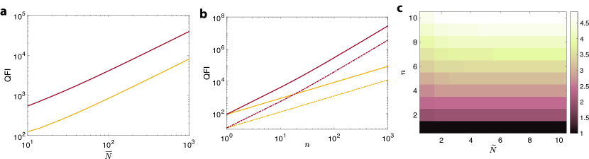
Figure 4: Comparison of QFI scaling of displacement sensing between the star graph state (maroon) and separable state (yellow) with respect to (a) $\mathrm{bar}N$ for fixed $n=10$ and (b) $n$ for fixed $\widetilde{N}=1$ (dash-dotted line) and $\widetilde{N}=10$ (solid line). (c) Ratio of QFI achieved by the star graph state and separable state for small $n$ and $\widetilde{N}$. We have chosen $f=1$.

We first consider again the simplified case with $f_{i}\equiv f$ for all quadratures. In this case, Eq. 21 reduces to

$$F(\phi|\hat{\rho})=2nf^{2}e^{2r}+2nf^{2}e^{-2r}+\sum_{i,j=1}^{n}4f^{2}e^{2r}A_{ij}+\sum_{i,j=1}^{n}2f^{2}e^{2r}[A^{2}]_{ij}.$$ (22)

We assume the leading terms in $F(\phi|\hat{\rho})$ and $\mathrm{bar}N$ are the adjacency matrix-dependent terms for a sufficiently connected graph. For the displacement sensing, we define another characteristic figure of a graph to be

$$\chi_{\textrm{d}}\equiv\frac{\sum\limits_{i,j=1}^{n}[A^{2}]_{ij}}{\Tr A^{2}},$$ (23)

with which the QFI can be expressed as

$$F(\phi|\hat{\rho})\approx 8f^{2}\chi_{\textrm{d}}\mathrm{bar}N\equiv 8f^{2}\chi_{\textrm{d}}\,n\widetilde{N}.$$ (24)

Since $[A^{2}]_{ij}$ is the number of common neighbors of the $i$-th and $j$-th vertices, it is obvious that $[A^{2}]_{ij}\leq\min\{\mathrm{deg}(i),\mathrm{deg}(j)\}\leq\sqrt{\mathrm{deg}(i)\mathrm{deg}(j)}$, where $\mathrm{deg}(i)$ is the degree of the $i$-th vertex. This leads to

$$\chi_{\textrm{d}} \leq\frac{\sum\limits_{i,j=1}^{n}\sqrt{\mathrm{deg}(i)\mathrm{deg}(j)}}{\mathrm{Tr}A^{2}}$$ (25)

$$\leq\frac{n\left[\sum\limits_{i,j=1}^{n}\mathrm{deg}(i)\mathrm{deg}(j)\right]^{\frac{1}{2}}}{\mathrm{Tr}A^{2}}$$

$$=\frac{n\sum\limits_{i=1}^{n}\mathrm{deg}(i)}{\mathrm{Tr}A^{2}}$$

$$=n,$$

where we have used the Cauchy-Schwartz inequality and the fact that $\Tr A^{2}=\sum\limits_{i=1}^{n}\mathrm{deg}(i)$. To asymptotically saturate the limit given by Eq. 25, or at least to realize the linear scaling in $n$ for $\chi_{\textrm{d}}$, we require $[A^{2}]_{ij}=\min\{\mathrm{deg}(i),\mathrm{deg}(j)\}=\sqrt{\mathrm{deg}(i)\mathrm{deg}(j)}=\textrm{const.}$ for most vertices in the graph, which means that the majority of vertices share the same neighbors. This indicates that the star graph state is again a good candidate. Another graph state satisfying this criterion is the $l-$multipartite graph (Appendix B).

For the star graph state, the characteristic figure and QFI are $\chi_{\textrm{d}}=\frac{n}{2}$ and $F(\phi|\hat{\rho})\approx 2n^{2}f^{2}e^{2r}\approx\frac{8}{3}f^{2}n\mathrm{bar}{N}=\frac{8}{3}f^{2}n^{2}\widetilde{N}$, respectively. Thus, the Heisenberg scaling over the number of modes (for fixed number of photons per mode) and the total number of photons is achieved. We stress that, in the displacement sensing, the Heisenberg scaling over total number of photons is linear in contrast to phase sensing. The separable state, on the other hand, has $F(\phi|\hat{\rho})\propto 2nf^{2}e^{2r}\approx 8f^{2}\mathrm{bar}N=8f^{2}n\widetilde{N}$, which only achieves the standard quantum limit in terms of the number of modes. We plot the QFI of phase sensing (calculated using Eq. 22) for the star graph state and separable state in Fig. 4. The star graph state always outperforms the separable state.

We now consider the general case with unequal $f_{j}$ for the star graph state. The QFI to the leading order is given by,

$$F(\phi|\hat{\rho}) \approx 2e^{2r}\left[\left(\sum_{j=1}^{n}f_{j+n}\right)^{2}+f_{n+1}\left(nf_{n+1}-2\sum_{j=1}^{n}f_{j+n}\right)\right]$$ (26)

$$\geq 2e^{2r}\left(n^{2}f_{\textrm{min}}^{2}+nf_{n+1}^{2}-2nf_{n+1}f_{\textrm{max}}\right),$$

where $f_{\textrm{min(max)}}=\textrm{min(max)}\{f_{n+1},\cdots,f_{2n}\}$ and we have labeled the center vertex of the graph to be $j=1$. Since $f_{j}$’s are independent of $n$ and $\mathrm{bar}N$, and assuming they do not vary significantly among different modes, we see that the Heisenberg scaling over the number of modes persists.

Similar to the phase sensing, we investigate whether the QFI can be saturated by the local homodyne detection. For the displacement sensing, we find the first- and second-order moment of the probability distribution of the outcome of homodyne measurement is given by

$$\omega_{i}=\phi([F_{2}]_{ii}f_{n+i}-[G_{2}]_{ii}f_{i})$$ (27)

and

$$\sigma_{M}=\frac{1}{2}\big{[}F_{2}U^{-1}F_{2}+G_{2}VU^{-1}F_{2}+F_{2}U^{-1}VG_{2}+G_{2}UG_{2}+G_{2}VU^{-1}VG_{2}\big{]},$$ (28)

respectively, where $F_{2}$ and $G_{2}$ are given by Eq. 18. The FI is then numerically calculated using Eq. 16 for the star graph state with $f_{i}\equiv f$. By varying the local oscillator phases $\alpha$ and $\beta$, as in the phase sensing, we find the optimized FI saturates the QFI (Fig. 5). This result suggests that local homodyne detection is able to achieve the optimal sensitivity predicted by the QFI for displacement sensing.

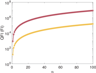
Figure 5: Numerically calculated FI (dots) of displacement sensing with the star graph state and the homodyne detection with optimized local oscillator phases, for $r=1$ (yellow) and 3 (maroon). The solid line shows the analytical QFI. Here, we have chosen $f=1$.

IV Conclusion and Discussion

In summary, we have investigated using CV graph states for quantum metrology, including both phase and displacement sensing that are of practical relevance. In particular, QFI of the two sensing modalities with general CV graph states is found, which can be benchmarked with characteristic factors intrinsic to the underlying graphs. With this, we identified the star graph states as an optimal resource which provides the Heisenberg scaling of the sensitivity over the number of modes for both phase and displacement sensing. Furthermore, we discovered that local homodyne detection is able to fulfill the QFI for phase and displacement sensing up to a constant factor, which makes this scheme based on CV graph states more appealing.

Compared with multi-mode metrology schemes where the probe states are prepared as the outcome of a highly squeezed state propagating through a mesh of beam splitters zhuang2018distributed ; guo2020distributed , the scheme using graph states faces similar difficulty of generating large amount of squeezing, here for the implementation of the $C_{z}$ gate. However, several methods have been proposed to generate graph states, including those based on linear optics van2007building ; su2007experimental , frequency combs menicucci2007ultracompact ; pysher2011parallel , QND gates menicucci2010arbitrarily , and photonic temporal modes menicucci2011temporal . With proof-of-principle demonstrations of some of these proposals realized recently yukawa2008experimental ; chen2014experimental ; roslund2014wavelength ; yokoyama2013ultra , the CV graph states discussed in this work represent a viable resource for distributed quantum sensing.

Appendix A Mean photon number of CV graph states

For a CV graph state with adjacency matrix $A$ created by the canonical method, its Wigner function is given by gu2009quantum

$$W(\vec{q},\vec{p}) =\frac{1}{\pi^{n}}\exp(-\sum_{j=1}^{n}q_{j}^{2}/s^{2})$$ (29)

$$\times\exp[-\sum_{j=1}^{n}s^{2}\left(p_{j}-\sum_{k=1}^{n}A_{jk}q_{k}\right)^{2}]$$

where $s\equiv e^{r}$. The mean photon number could be calculated using

$$\mathrm{bar}{N}=\int\int d\vec{q}\,d\vec{p}\,W(\vec{q},\vec{p})\sum_{i=1}^{n}\frac{1}{2}(q_{i}^{2}+p_{i}^{2}-1),$$ (30)

which yields

$$\mathrm{bar}{N}=n\sinh^{2}r+\frac{1}{4}e^{2r}\Tr A^{2}.$$ (31)

Appendix B Other examples of graph states

We calculate the QFI of some other graph states for phase and displacement sensing.

$l$-multipartite graph states: The vertices of this type of graph states can be partitioned into $l$ sets and the vertices in each set are only connected with all vertices out of this set. Assuming each set has $m$ vertices, its adjacency matrix can be written as $A=A^{\prime}\otimes G$, where $A^{\prime}_{ij}=1-\delta_{ij}$, $1\leq i,j\leq l$, and $G_{kl}=1$, $1\leq k,l\leq m$. $A$ has two nonzero eigenvalues: $(l-1)m$ (1-fold) and $=-m$ ($(l-1)$-fold). As a result, we find $\chi_{\textrm{p}}=\frac{l-1}{l}\approx 1$ and $\chi_{\textrm{d}}=m(l-1)\approx n$, which is similar to the star graph.

Rectangular graph states: The corresponding graph resembles a belt formed by squares. Consider the $4\times m$ rectangular graph state with $n=4m$ modes. It has an adjacency matrix $A_{ij}=\delta_{i,j-1}+\delta_{i,j+1}+\delta_{i,j+4}+\delta_{i,j-4}$. In the large $n$ limit, $\Tr A^{2}=4n$, $\Tr A^{4}=36n-84$, and $\sum\limits_{i,j=1}^{n}[A^{2}]_{ij}=16n$. As a result, $\chi_{\textrm{p}}=\frac{36n-84}{16n^{2}}\approx\frac{9}{4n}$ and $\chi_{\textrm{d}}=4$, leading to worse scaling than star and $l$-multipartite graph states.

References

- (1) Giovannetti, V., Lloyd, S. & Maccone, L. Quantum-enhanced measurements: beating the standard quantum limit. Science 306, 1330–1336 (2004).
- (2) Giovannetti, V., Lloyd, S. & Maccone, L. Quantum metrology. Physical Review Letters 96, 010401 (2006).
- (3) Degen, C. L., Reinhard, F. & Cappellaro, P. Quantum sensing. Reviews of Modern Physics 89, 035002 (2017).
- (4) Pirandola, S., Bardhan, B. R., Gehring, T., Weedbrook, C. & Lloyd, S. Advances in photonic quantum sensing. Nature Photonics 12, 724 (2018).
- (5) Abadie, J. et al. A gravitational wave observatory operating beyond the quantum shot-noise limit. Nature Physics 7, 962 (2011).
- (6) Aasi, J. et al. Enhanced sensitivity of the ligo gravitational wave detector by using squeezed states of light. Nature Photonics 7, 613 (2013).
- (7) Holland, M. & Burnett, K. Interferometric detection of optical phase shifts at the heisenberg limit. Physical Review Letters 71, 1355 (1993).
- (8) Mitchell, M. W., Lundeen, J. S. & Steinberg, A. M. Super-resolving phase measurements with a multiphoton entangled state. Nature 429, 161–164 (2004).
- (9) Humphreys, P. C., Barbieri, M., Datta, A. & Walmsley, I. A. Quantum enhanced multiple phase estimation. Physical Review Letters 111, 070403 (2013).
- (10) Anisimov, P. M. et al. Quantum metrology with two-mode squeezed vacuum: parity detection beats the heisenberg limit. Physical Review Letters 104, 103602 (2010).
- (11) Zhuang, Q., Zhang, Z. & Shapiro, J. H. Distributed quantum sensing using continuous-variable multipartite entanglement. Physical Review A 97, 032329 (2018).
- (12) Matsubara, T., Facchi, P., Giovannetti, V. & Yuasa, K. Optimal gaussian metrology for generic multimode interferometric circuit. New Journal of Physics 21, 033014 (2019).
- (13) Guo, X. et al. Distributed quantum sensing in a continuous-variable entangled network. Nature Physics 16, 281–284 (2020).
- (14) Rosenkranz, M. & Jaksch, D. Parameter estimation with cluster states. Physical Review A 79, 022103 (2009).
- (15) Friis, N. et al. Flexible resources for quantum metrology. New Journal of Physics 19, 063044 (2017).
- (16) Shettell, N. & Markham, D. Graph states as a resource for quantum metrology. Physical Review Letters 124, 110502 (2020).
- (17) Paris, M. G. Quantum estimation for quantum technology. International Journal of Quantum Information 7, 125–137 (2009).
- (18) Tóth, G. & Apellaniz, I. Quantum metrology from a quantum information science perspective. Journal of Physics A: Mathematical and Theoretical 47, 424006 (2014).
- (19) Weedbrook, C. et al. Gaussian quantum information. Reviews of Modern Physics 84, 621 (2012).
- (20) Simon, R., Sudarshan, E. & Mukunda, N. Gaussian pure states in quantum mechanics and the symplectic group. Physical Review A 37, 3028 (1988).
- (21) Menicucci, N. C., Flammia, S. T. & van Loock, P. Graphical calculus for gaussian pure states. Physical Review A 83, 042335 (2011).
- (22) Adesso, G., Ragy, S. & Lee, A. R. Continuous variable quantum information: Gaussian states and beyond. Open Systems & Information Dynamics 21, 1440001 (2014).
- (23) Kay, S. M. Fundamentals of statistical signal processing (Prentice Hall PTR, 1993).
- (24) van Loock, P., Weedbrook, C. & Gu, M. Building gaussian cluster states by linear optics. Physical Review A 76, 032321 (2007).
- (25) Su, X. et al. Experimental preparation of quadripartite cluster and greenberger-horne-zeilinger entangled states for continuous variables. Physical Review Letters 98, 070502 (2007).
- (26) Menicucci, N. C., Flammia, S. T., Zaidi, H. & Pfister, O. Ultracompact generation of continuous-variable cluster states. Physical Review A 76, 010302 (2007).
- (27) Pysher, M., Miwa, Y., Shahrokhshahi, R., Bloomer, R. & Pfister, O. Parallel generation of quadripartite cluster entanglement in the optical frequency comb. Physical Review Letters 107, 030505 (2011).
- (28) Menicucci, N. C., Ma, X. & Ralph, T. C. Arbitrarily large continuous-variable cluster states from a single quantum nondemolition gate. Physical Review Letters 104, 250503 (2010).
- (29) Menicucci, N. C. Temporal-mode continuous-variable cluster states using linear optics. Physical Review A 83, 062314 (2011).
- (30) Yukawa, M., Ukai, R., Van Loock, P. & Furusawa, A. Experimental generation of four-mode continuous-variable cluster states. Physical Review A 78, 012301 (2008).
- (31) Chen, M., Menicucci, N. C. & Pfister, O. Experimental realization of multipartite entanglement of 60 modes of a quantum optical frequency comb. Physical Review Letters 112, 120505 (2014).
- (32) Roslund, J., De Araujo, R. M., Jiang, S., Fabre, C. & Treps, N. Wavelength-multiplexed quantum networks with ultrafast frequency combs. Nature Photonics 8, 109 (2014).
- (33) Yokoyama, S. et al. Ultra-large-scale continuous-variable cluster states multiplexed in the time domain. Nature Photonics 7, 982 (2013).
- (34) Gu, M., Weedbrook, C., Menicucci, N. C., Ralph, T. C. & van Loock, P. Quantum computing with continuous-variable clusters. Physical Review A 79, 062318 (2009).