Cucker-Smale type flocking models on a sphere

Abstract.

We present a Cucker-Smale (C-S) type flocking model on a sphere. We study velocity alignment on a sphere and prove the emergence of flocking for the proposed model. Our model includes three new terms: a centripetal force, multi-agent interactions on a sphere and inter-particle bonding forces. To compare velocity vectors on different tangent spaces, we introduce a rotation operator in our new interaction term. Due to the geometric restriction, the rotation operator is singular at antipodal points and the relative velocity between two agents located at these points is not well-defined. Based on an energy dissipation property of our model and a variation of Barbalat’s lemma, we show the alignment of velocities for an admissible class of communication weight functions. In addition, for sufficiently large bonding forces we prove time-asymptotic flocking which includes the avoidance of antipodal points.

1. Introduction

Collective behaviors are ubiquitous phenomena in nature. Many organisms employ collective behaviors to survive in nature: examples include the aggregation of bacteria, the flocking of birds and fish schools. Recently, these phenomena have been intensively studied in engineering communities due to their applications. In engineering, a model with a constant speed is preferred for practical reasons and control problems are often addressed. For instance, in [15, 16], Justh and Krishnaprasad considered a unit speed particle model satisfying a Frenet-Serret equation with curvature control. Generalizations of a discrete time Vicsek model with leadership and without leadership were discussed in [14]. A planar model that has a gyroscopic steering force with unit speed was studied in [26]. Their coupling depends on the position and angle of velocity. Leonard et al. designed a particle motion control to collect information in [19]. They focused on developing and solving an optimal control problem for cost functions.

In the mathematics and physics communities, many researchers have also studied these phenomena in various perspectives and in various forms. For examples, Topaz and Bertozzi considered a fluid type model describing social interaction in two spatial dimensions and studied swarming patterns in [31]. Their model contains a nonlocal velocity alignment term. In [10], Fetecau and Eftimie presented a discrete velocity model with a nonlocal force and turning rate. They considered the global existence and aggregation phenomena. Especially, after the mathematical model of Winfree and Kuramoto for collective dynamics [17, 18, 33], many researchers have proposed agent-based models to study the emergent behaviors analytically and numerically. Vicsek et al. in [32] proposed a second-order flocking model with discrete time scheme, the so-called Vicsek model. In this model, all agents in the system have a constant speed. We refer to [7, 9, 30] for noise and position dependent force, derivation of a macroscopic model with a diffusion coefficient, and a statistical view point, respectively.

In this paper, we continue to study the flocking model from Cucker and Smale [6], which is a kind of $N$-body system. Cucker and Smale [6] introduced a system of ordinary differential equations such that acceleration is described by weighted internal relaxation forces:

$$\begin{aligned} \frac{dx_{i}}{dt}&=v_{i},\\ \frac{dv_{i}}{dt}&=\sum_{j=1}^{N}\frac{\psi_{ij}}{N}(v_{j}-v_{i}),\end{aligned}$$ (1.1)

where $x_{i}$ and $v_{i}$ are the position and velocity in $\mathbb{R}^{d}$ of the $i$th agent, respectively, and $\psi_{ij}$ is the communication rate between the $i$th and $j$th agents. Cucker and Smale [6] also provided sufficient conditions for initial data leading to flocking configuration. We refer to [1, 3, 12, 13, 24, 25] for results related to C-S models.

While the original C-S model (1.1) describes $N$-body agents in $\mathbb{R}^{d}$, collective behaviors can occur on other manifolds. For example, all living organisms in nature are located in the Earth and the geometry of the Earth may not be negligible in long-distance travel. We provide a brief historical remark of flocking dynamics on manifolds. The Kuramoto model in [17, 18] is a first-order differential equation type model, and the oscillators are arranged in $\mathbb{S}^{1}$. Lohe generalized the Kuramoto model to a matrix model in [20, 21]. From the matrix model, Lohe derived a dynamical model in $\mathbb{S}^{4}$ that was inspired by quantum information theory. The ellipsoid model was studied in [34]. Vicsek and his collaborators in [32] considered the second-order discrete time model with $v\in\mathbb{S}^{1}$. See [11] for the continuous time model and [5] for general dimension cases.

The main objective of this paper is to derive a C-S type flocking model on a unit sphere. Additionally, we need a new definition of flocking for the model to describe the flocking phenomena on a sphere. The main difficulty comes from analysis of the velocity difference, a so-called relative velocity, on a manifold. The concept of a relative velocity on a manifold has been well-developed and widely used in general relativity (See [4, 22, 28, 29]). The relative velocity can be considered as parallel transport along geodesics (See [4, Equation (3.109)]). On a sphere, a geodesic is a part of a great circle and a parallel transport along a great circle is characterized by a rotation matrix, given in Definition 2.1. Furthermore, as our domain is not a Euclidean domain but a unit sphere, the classical Lyapunov functional approach which provides an exponential convergence rate in the previous articles cannot be applied directly. Instead, we use an integrable system property to obtain the flocking result.

The model proposed in this paper is an agent-based Newton’s equation type model as the original C-S model. We assume that each particle has unit mass. Consider an ensemble of agents on a unit sphere. Let $x_{i},v_{i}\in\mathbb{R}^{3}$ be the position and momentum of the $i$th agent respectively. Note that $x_{i}$ is a unit vector corresponding to the position on the unit sphere. Because of the geometric restrictions, we need an extra term to conserve the modulus of $x_{i}$, called the centripetal force. In the original C-S model, the sum of velocity differences between two particles is considered as acceleration. Since the surface is not flat in our model, we cannot obtain a relative velocity between the other two agents by a simple vector difference. More precisely, if we simply take the difference $v_{i}-v_{j}$ between $i$th and $j$th agents as the relative velocity, then it may not be contained in the tangent space of the given position vector $x_{i}$ at time $t>0$. Therefore, we need a new interaction rule between the two velocities $v_{i}$ and $v_{j}$.

The result of this paper are threefold. First, we derive a C-S type system on a unit sphere, based on the original C-S model (1.1), by using the centripetal force, a rotation operator, and an inter-particle bonding force. The following system of first-order ordinary differential equations is a counterpart of the C-S model on the unit sphere: for $x_{i},v_{i}\in\mathbb{R}^{3}$ and $i=1,\ldots,N$,

$$\begin{aligned} \dot{x}_{i}&=v_{i},\\ \dot{v}_{i}&=-\frac{\|v_{i}\|^{2}}{\|x_{i}\|^{2}}x_{i}+\sum_{j=1}^{N}\frac{\psi_{ij}}{N}\big{(}R_{x_{j}\shortrightarrow x_{i}}(v_{j})-v_{i}\big{)}+\sum_{k=1}^{N}\frac{\sigma}{N}(\|x_{i}\|^{2}x_{k}-\langle x_{i},x_{k}\rangle x_{i}),\end{aligned}$$ (1.2)

where $\psi_{ij}=\psi(\|x_{i}-x_{j}\|)$ is the communication rate and $\sigma$ is the inter-particle bonding parameter. Here, $R_{x_{1}\shortrightarrow x_{2}}(y)$ is the rotation operator, which consists of a matrix $R(x_{1},x_{2})$ and its matrix product (See Definition 2.1). The detailed definition and properties of the operator $R_{x_{1}\shortrightarrow x_{2}}(y)$ are discussed in Section 2. We refer to [8, 23] for C-S models on $\mathbb{T}^{d}$.

(a) $t=0$

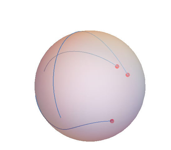
(b) $t=1$

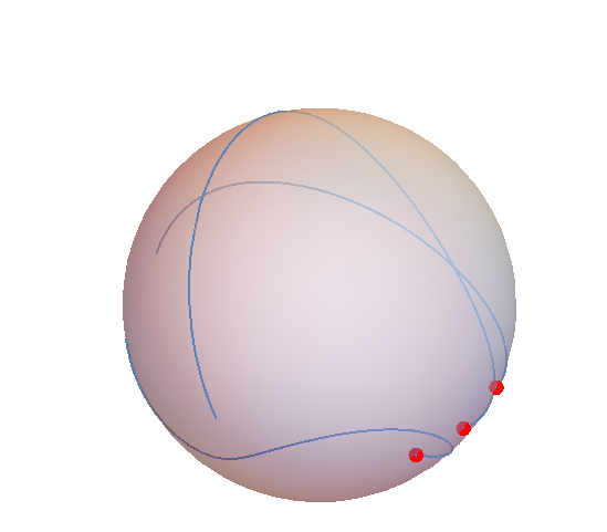
(c) $t=2$

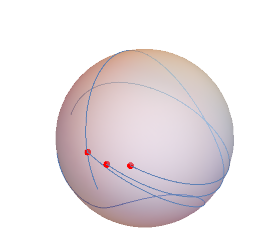
(d) $t=3$

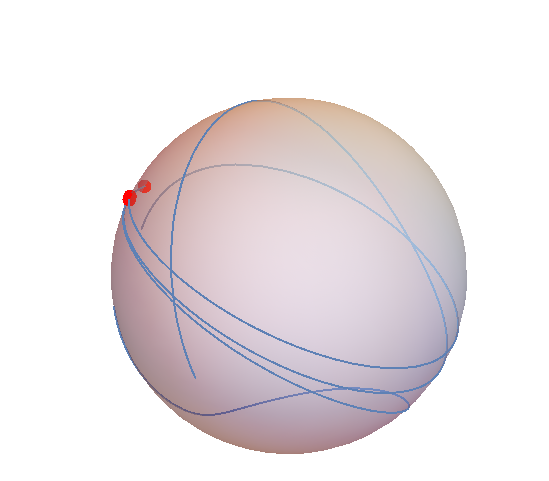
(e) $t=4$

(f) $t=5$

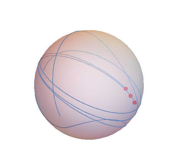
(g) $t=6$

(h) $t=7$

(i) $t=8$

Figure 1. Numerical experiment of flocking on a unit sphere for three particles.

In the original C-S model [6], the communication rate $\psi_{ij}=\psi(\|x_{i}-x_{j}\|)$ quantifies how the agents affect each other and $\psi$ is a decreasing function of distance $\|x_{i}-x_{j}\|$ between two agents $x_{i}$ and $x_{j}$. The main concern in system (1.2) is to determine $\psi_{ij}$ when two points $x_{i}$ and $x_{j}$ in $\mathbb{S}^{2}$ are antipodal. As there are infinitely many geodesics connecting two antipodal points in $\mathbb{S}^{2}$, it is unclear what effect the corresponding antipodal point has. Rather, it is natural to assume that the influence of one agent on another agent is negligible if their positions are antipodal. To illustrate this, we assume that $\psi_{ij}=\psi(\|x_{j}-x_{i}\|)$ and

$$\hbox{ a decreasing $C^{1}$ function }\psi:[0,2]\to[0,+\infty)\hbox{ satisfies }\psi(2)=0\hbox{ and }\psi^{\prime}(2)<0.$$ (1.3)

Second, we develop flocking on a unit sphere as follows.

Definition 1.1.

A system has time-asymptotic flocking on a sphere in $\mathbb{R}^{3}$ if and only if a solution $(x_{i},v_{i})_{i=1}^{N}$ of the system satisfies the following condition:

• (velocity alignment) the relative velocity on the unit sphere goes to zero time-asymptotically:

  $$\lim_{t\rightarrow\infty}\max_{1\leq i,j\leq N}\|x_{i}(t)+x_{j}(t)\|\|R_{x_{j}(t)\shortrightarrow x_{i}(t)}(v_{j}(t))-v_{i}(t)\|=0.$$

• (antipodal points avoidance) any two agent are not located at the antipodal points:

  $$\liminf_{t\geq 0}\min_{1\leq i,j\leq N}\|x_{i}(t)+x_{j}(t)\|>0.$$

It is worth noting that Definition 1.1 has the avoidance of antipodal points while the boundedness of position fluctuations is included in the original definition of flocking in $\mathbb{R}^{3}$. As the domain is compact in our case, the boundedness condition for the position difference $x_{i}-x_{j}$ does not guarantee the formation of a group. Instead, the avoidance of antipodal points is required because antipodal points are as far away from each other as possible.

The rotation operator from one point to its antipodal point cannot be defined (See Remark 2.3(2)). For this reason, the relative velocity will be only considered if points are not antipodal. In fact, the conditions below

$$\lim_{t\rightarrow+\infty}\|x_{i}(t)+x_{j}(t)\|\|R_{x_{j}(t)\shortrightarrow x_{i}(t)}(v_{j}(t))-v_{i}(t)\|^{k}=0$$

are equivalent for any $k>0$ as long as $v_{i}$ and $v_{j}$ are uniformly bounded in time (See Lemma C.1). The simplest example of flocking on a sphere is a set of unit speed circular motions.

Example 1.1.

For $t\geq 0$ and $1\leq i\leq N$, consider

$$x_{i}(t):=(\cos(t+\alpha_{i}),\sin(t+\alpha_{i}),0),\quad v_{i}(t):=(-\sin(t+\alpha_{i}),\cos(t+\alpha_{i}),0)\hbox{ and }0\leq\alpha_{i}<\pi.$$ (1.4)

By direct computation, it holds that for all $t\geq 0$ and $1\leq i\leq N$,

$$R_{x_{j}(t)\shortrightarrow x_{i}(t)}(y)=\left(\begin{matrix}\cos(\alpha_{i}-\alpha_{j})&-\sin(\alpha_{i}-\alpha_{j})&0\\ \sin(\alpha_{i}-\alpha_{j})&\cos(\alpha_{i}-\alpha_{j})&0\\ 0&0&1\end{matrix}\right)y.$$

Thus, we have $R_{x_{j}(t)\shortrightarrow x_{i}(t)}(v_{j}(t))=v_{i}(t)$ for all $t\geq 0$, and $(x_{i},v_{i})_{i=1}^{N}$ given in (1.4) satisfies the conditions in Definition 1.1.

Third, we provide the global-in-time existence and flocking result for an admissible class of communication weight functions. To obtain the flocking estimate for the solution to (1.2), we consider the following total energy functional $\mathcal{E}$ given by the sum of the kinetic energy $\mathcal{E}_{K}$ and configuration energy $\mathcal{E}_{C}$ motivated by [27]: for a given ensemble $(x_{i},v_{i})_{i=1}^{N}$, we define energy functional $\mathcal{E}(x(t),v(t))$ such as

$$\mathcal{E}:=\mathcal{E}_{K}+\mathcal{E}_{C},\quad\mathcal{E}_{K}(t):=\frac{1}{N}\sum_{k=1}^{N}\|v_{k}(t)\|^{2},\quad\mathcal{E}_{C}(t):=\frac{\sigma}{2N^{2}}\sum_{k,l=1}^{N}\|x_{k}(t)-x_{l}(t)\|^{2}.$$ (1.5)

If the bonding force rate $\sigma$ is large enough comparing the differences of agents’ velocities and positions, then the following flocking result holds. What follows is a summary of our results from Theorem 3.1, Theorem 4.4 and Theorem  4.7.

Theorem 1.

For $\psi$ satisfying (1.3) and $\sigma\geq 0$, there exists a unique global solution to (1.2) and the system in (1.2) has the velocity alignment on a sphere. Moreover, for $\sigma>N^{2}\mathcal{E}(0)/2$, the solution to (1.2) has time-asymptotic flocking on a unit sphere. Here, $\mathcal{E}(0)$ is the initial energy of the system given in (1.5).

We note that it remains open to show the emergence of flocking for $\sigma=0$ and the complete position flocking for $\sigma>0$. For the original C-S model defined in a flat space, the a priori assumption that the spatial diameter of agents is uniformly bounded yields an exponential decay for the maximum velocity differences between agents. Conversely, the exponential decay of the maximum velocity differences also leads to the uniform boundedness of the position difference. From this a priori estimate argument, the emergence of the flocking for the original C-S model is attained. However, this standard methodology is not applicable to our model on the sphere.

The main difficulty comes from estimating the position difference between two agents. We expect that the exponential decay of the relative velocity $\|R_{x_{j}\shortrightarrow x_{i}}(v_{j})-v_{i}\|$ yields the boundedness of the position difference. However, in our case since the sphere is a curved space, $R_{x_{j}\shortrightarrow x_{i}}$ depends on agents’ location. Thus, unlike the original C-S model, it is not clear whether there is a Gronwall-type dissipative differential inequality for the relative velocity, even assuming a priori that the position difference at $t=0$ is small.

The rest of this paper is organized as follows. In Section 2, we present a derivation of the C-S type model (1.2) on the unit sphere from the original C-S model. In Section 3, we provide the global well-posedness of the solution to the derived model (1.2). In Section 4, we prove the asymptotic flocking theorem for the system. Finally, Section 5 is devoted to the summary of our main results.

Notation: For given $z\in\mathbb{R}^{3}$, we use the symbols $\|z\|$ and $\|z\|_{\infty}$ to denote the $\ell_{2}$-norm and $\ell_{\infty}$-norm, respectively. For three-dimensional vectors $y$ and $z$, we denote the standard inner product between $y$ and $z$ as $\langle y,z\rangle$.

2. Motivation and derivation of the C-S type model on a sphere

2.1. Derivation

In this section, we present a derivation of the C-S type flocking model on a sphere. After normalization, we can assume that the domain is a unit sphere:

$$\mathbb{S}^{2}=\{(a_{1},a_{2},a_{3})\in\mathbb{R}^{3}:a_{1}^{2}+a_{2}^{2}+a_{3}^{2}=1\}.$$

We first consider the classical form of the C-S model in $\mathbb{R}^{3}$.

$$\dot{x}_{i} =v_{i},$$

$$\dot{v}_{i} =\sum_{j=1}^{N}\frac{\psi_{ij}}{N}(v_{j}-v_{i}).$$

Here, $x_{i}$ and $v_{i}$ represent the position and velocity of the $i$th agent, respectively, and $\psi_{ij}=\psi(\|x_{i}-x_{j}\|)$ is the communication rate or weight function for the interaction between $i$th and $j$th agents. In the original C-S model, the communication rate $\psi$ has a key role in the emergence of flocking as a control parameter. Note that to obtain global flocking result in the original C-S model, the power of denominator is important, i.e., if $\psi(x)=1/(1+|x|^{2})^{\beta/2}$, the following statement holds.

1. $\beta\in[0,1]$, unconditional flocking occurs,

2. $\beta\in(1,\infty)$, conditional flocking occurs.

Remark 2.1.

Unlike in the case of $\mathbb{R}^{3}$, the flocking model on the unit sphere does not require the long-range communications for unconditional flocking. On the other hand, since it has singularity in the antipodal positions, a vanishing condition in the antipodal positions such as (1.3) is required.

In the following, we construct a C-S type flocking model on a unit sphere that shares the same structure as the original C-S model, including the communication rate and velocity difference. Essentially, the C-S flocking model consists of three components: (1) the classic relation between the position $x_{i}$ and velocity $v_{i}$ in the first equation, $\dot{x}_{i}=v_{i}$, (2) the velocity difference $v_{j}-v_{i}$ in the second equation, and (3) the communication rate $\psi_{ij}$.

For the first trial, we fix the first two components and we try to find $\psi_{ij}$ to conserve the modulus of $x_{i}$. To make dynamics on the sphere, we need to obtain

$$\|x_{i}\|\equiv 1,\quad\mbox{for all time}~{}t>0.$$ (2.1)

If we have compatible initial data $x_{i}(0)$ and $v_{i}(0)$, an equivalent relation to the above is

$$\langle x_{i},v_{i}\rangle\equiv 0,\quad\mbox{for all time}~{}t>0.$$ (2.2)

Under this compatible initial condition, we can also obtain another equivalent relation as follows:(2.2)

$$\langle x_{i}(t),\dot{v}_{i}(t)\rangle+\|v_{i}(t)\|^{2}\equiv 0,\quad\mbox{for all time}~{}t>0,$$ (2.3)

and

$$\langle x_{i}(0),v_{i}(0)\rangle=0.$$ (2.4)

For the details, see Proposition 3.2.

Proposition 2.2.

Let $\psi_{ij}$ be scalar functions depending on $\{x_{1},\cdots,x_{N}\}$ for all $i,j\in\{1,\ldots,N\}$. Then a solution to the C-S flocking model (1.1) with communication rate $\psi_{ij}$ lying on the unit sphere does not exist.

Proof.

We assume that each agent lies on a unit sphere, i.e., for all $1\leq i\leq N$,

$$x_{i}\in\mathbb{S}^{2}.$$

Assume that the solution $(x_{i},v_{i})_{i=1}^{N}$ to the following C-S type equation is as follows:

$$\dot{x}_{i} =v_{i},$$

$$\dot{v}_{i} =\sum_{j=1}^{N}\frac{\psi_{ij}}{N}(v_{j}-v_{i}),$$

and take the inner product between $\dot{v}_{i}$ and $x_{i}$ to obtain

$$\langle\dot{v}_{i},x_{i}\rangle =\sum_{j=1}^{N}\frac{\psi_{ij}}{N}\langle v_{j}-v_{i}~{},x_{i}\rangle.$$

Note that from the argument in (2.1)-(2.4), we have

$$\langle x_{i},v_{i}\rangle\equiv 0$$

and

$$\langle x_{i},\dot{v}_{i}\rangle+\|v_{i}\|^{2}\equiv 0.$$

It follows that

$$-\|v_{i}\|^{2}=\langle\dot{v}_{i},x_{i}\rangle=\sum_{j=1}^{N}\frac{\psi_{ij}}{N}\langle v_{j}-v_{i}~{},x_{i}\rangle=\sum_{j=1}^{N}\frac{\psi_{ij}}{N}\langle v_{j}~{},x_{i}\rangle.$$

As $\psi_{ij}$ does not depend on $\{v_{1},\cdots,v_{N}\}$, the above equation holds for any $v_{i}$ such that $\langle v_{i},x_{i}\rangle=0$. Therefore, there is no such solution $\psi_{ij}$ to the equation. ∎

If we do not change the first equation, the only possibility to construct a unit sphere model is modification of the $v_{j}-v_{i}$ terms for $i,j\in\{1,\ldots,N\}$. As mentioned in Section 1, from geometrical consideration, it is natural to consider a relative velocity to keep all agents’ positions within the given manifold. However, without interactions between each agent, the positions of each agent are not maintained in the manifold. Therefore, we need an additional external force term. In the sense of (2.1) - (2.4), the acceleration $\dot{v}_{i}$ in our model has to satisfy

$$\langle x_{i},\dot{v}_{i}\rangle=-\|v_{i}\|^{2}.$$

We propose one possible model as follows. We add a self-consistency term, the so-called centripetal force, as $\displaystyle-\frac{\|v_{i}\|^{2}}{\|x_{i}\|^{2}}x_{i}$. Consider the following centripetal equation:

$$\dot{v}_{i}=-\frac{\|v_{i}\|^{2}}{\|x_{i}\|^{2}}x_{i}.$$

It is well known that the solution to the centripetal equation gives uniform circular motion on a sphere. Then, the remaining interaction term for the $i$th agent between agents must be orthogonal to $x_{i}$. Thus, we need an operator map from the tangent space of $x_{j}$ to the tangent space of $x_{i}$.

2.2. Model

Our proposed model is as follows: for $x_{i},v_{i}\in\mathbb{R}^{3}$ and $i=1,\ldots,N$,

$$\begin{aligned} \dot{x}_{i}&=v_{i},\\ \dot{v}_{i}&=-\frac{\|v_{i}\|^{2}}{\|x_{i}\|^{2}}x_{i}+\sum_{j=1}^{N}\frac{\psi_{ij}}{N}\big{(}R_{x_{j}\shortrightarrow x_{i}}(v_{j})-v_{i}\big{)}+\sum_{k=1}^{N}\frac{\sigma}{N}(\|x_{i}\|^{2}x_{k}-\langle x_{i},x_{k}\rangle x_{i}).\end{aligned}$$

Here, $R_{x_{1}\shortrightarrow x_{2}}(y)=R(x_{1},x_{2})\cdot y$ is the rotation operator defined below and $\sigma>0$ is the rate of the inter-particle bonding force.

Definition 2.1.

Let $x_{1},x_{2}\in\mathbb{S}^{2}$ be column vectors with $x_{1}\neq-x_{2}$. We define a $3\times 3$ matrix

$$R(x_{1},x_{2}):=\left\{\begin{aligned} &\langle x_{1},x_{2}\rangle I-x_{1}x_{2}^{T}+x_{2}x_{1}^{T}+(1-\langle x_{1},x_{2}\rangle)\Big{(}\frac{x_{1}\times x_{2}}{|x_{1}\times x_{2}|}\Big{)}\Big{(}\frac{x_{1}\times x_{2}}{|x_{1}\times x_{2}|}\Big{)}^{T},\quad&\mbox{if}\quad x_{1}\neq x_{2},\\ &I,\quad&\mbox{if}\quad x_{1}=x_{2},\end{aligned}\right.$$

where $I$ is the identity matrix in $\mathbb{R}^{3}$ and $M^{T}$ is the transpose of a matrix $M$. The operation $R_{x_{1}\shortrightarrow x_{2}}(y)$ is defined by the linear transform as

$$R_{x_{1}\shortrightarrow x_{2}}(y)=R(x_{1},x_{2})\cdot y.$$

Here, $y$ is a column vector and $\cdot$ is the matrix product. Furthermore, we set

$$\|x_{1}+x_{2}\|R(x_{1},x_{2}):=0\hbox{ at }x_{1}=-x_{2}.$$

Remark 2.3.

1. By direct calculation, we can rewrite the rotation matrix as

   $$R(x_{1},x_{2})=\cos\theta~{}I+\sin\theta~{}[{\bf u}]+(1-\cos\theta)~{}{\bf u}\otimes{\bf u},$$ (2.5)

   where $\displaystyle{\bf u}=\frac{x_{1}\times x_{2}}{\|x_{1}\times x_{2}\|}$ is the normalized cross product between the vectors $x_{1}$ and $x_{2}$, $\theta$ is the angle between $x_{1}$ and $x_{2}$, and $[{\bf u}]$, ${\bf u}\otimes{\bf u}$ are given by

   $$[{\bf u}]=\left(\begin{matrix}0&-u_{e_{3}}&u_{e_{2}}\\ u_{e_{3}}&0&-u_{e_{1}}\\ -u_{e_{2}}&u_{e_{1}}&0\end{matrix}\right),\quad{\bf u}\otimes{\bf u}=\left(\begin{matrix}u_{e_{1}}^{2}&u_{e_{1}}u_{e_{2}}&u_{e_{1}}u_{e_{3}}\\ u_{e_{1}}u_{e_{2}}&u_{e_{2}}^{2}&u_{e_{2}}u_{e_{3}}\\ u_{e_{1}}u_{e_{3}}&u_{e_{2}}u_{e_{3}}&u_{e_{3}}^{2}\end{matrix}\right).$$

   Here, $u_{e_{1}}$, $u_{e_{2}}$ and $u_{e_{3}}$ are the first, second and third components of the vector $u$, respectively.

2. For $x_{1}=-x_{2}$, the third term in the right-hand side of (2.5) is not well-defined. Geometrically, if two points are located at opposite poles (for example, the north pole and south pole), then there are infinitely many geodesics connecting the two points. This means that we cannot determine a unique parallel transport. From this property, we need to take $\psi_{ij}=\psi(\|x_{i}-x_{j}\|)$ with some decay assumption at $x_{1}=-x_{2}$. Thus, the model (1.2) is valid although $R(x_{1},x_{2})$ is not defined at $x_{1}=-x_{2}$. Our assumptions on $\psi_{ij}$ and the well-posedness will be shown later.

3. For any $x_{1}\in\mathbb{S}^{2}$, it holds that

   $$\lim_{x_{2}\to x_{1}}R(x_{1},x_{2})=I.$$

4. Note that $R(x_{1},x_{2})$ is bounded for any $x_{1},x_{2}\in\mathbb{S}^{2}$ (See Lemma 2.5). Thus, although $R(x_{1},x_{2})$ is not defined at $x_{1}=-x_{2}$, it is natural to define $\|x_{1}+x_{2}\|R(x_{1},x_{2})=0$ at $x_{1}=-x_{2}$.

Next, we provide elementary properties of the rotation matrix.

Lemma 2.4.

For $x_{1},x_{2}\in\mathbb{S}^{2}$ with $x_{1}\neq-x_{2}$, the following holds.

$$R_{x_{1}\shortrightarrow x_{2}}(x_{1})=x_{2},\quad R_{x_{1}\shortrightarrow x_{2}}(x_{2})=2\langle x_{1},x_{2}\rangle x_{2}-x_{1}~{}\hbox{ and }~{}R_{x_{1}\shortrightarrow x_{2}}(x_{1}\times x_{2})=x_{1}\times x_{2}.$$

Furthermore, we have

$$R_{x_{1}\shortrightarrow x_{2}}^{T}=R_{x_{2}\shortrightarrow x_{1}},\quad R_{x_{1}\shortrightarrow x_{2}}^{T}\circ R_{x_{1}\shortrightarrow x_{2}}=I_{\mathbb{S}^{2}}.$$

Proof.

By definition of the rotation map $R_{x_{1}\shortrightarrow x_{2}}:\mathbb{S}^{2}\shortrightarrow\mathbb{S}^{2}$, it is enough to consider the equivalent properties for a matrix $R(x_{1},x_{2})$ defined in Definition 2.1. For the case of $x_{1}=x_{2}$, we can easily check that $R(x_{1},x_{2})$ satisfies Lemma 2.4, since $R(x_{1},x_{2})=I$.

Next, we consider the case, $x_{1}\neq x_{2}$. As the two vectors $x_{1}$ and $x_{2}$ are perpendicular to $x_{1}\times x_{2}$, direct computation shows that

$$R(x_{1},x_{2})\cdot x_{1}=x_{2},\quad R(x_{1},x_{2})\cdot x_{2}=2\langle x_{1},x_{2}\rangle x_{2}-x_{1}\hbox{ and }R(x_{1},x_{2})\cdot(x_{1}\times x_{2})=x_{1}\times x_{2}.$$ (2.6)

Furthermore, since we have

$$\begin{aligned} R(x_{1},x_{2})^{T}&=\langle x_{1},x_{2}\rangle I-x_{2}x_{1}^{T}+x_{1}x_{2}^{T}+(1-\langle x_{1},x_{2}\rangle)\left(\frac{x_{1}\times x_{2}}{|x_{1}\times x_{2}|}\right)\left(\frac{x_{1}\times x_{2}}{|x_{1}\times x_{2}|}\right)^{T},\end{aligned}$$

we conclude that

$$R(x_{1},x_{2})^{T}=R(x_{2},x_{1}).$$ (2.7)

We show that $R(x_{1},x_{2})$ is an orthogonal matrix, that is

$$R(x_{1},x_{2})^{T}R(x_{1},x_{2})=I.$$ (2.8)

From (2.6) and (2.7), it holds that

$$R(x_{1},x_{2})^{T}R(x_{1},x_{2})\cdot x_{1}=R(x_{2},x_{1})\cdot x_{2}=x_{1}$$

and

$$R(x_{1},x_{2})^{T}R(x_{1},x_{2})\cdot x_{2}=R(x_{2},x_{1})\cdot(2\langle x_{1},x_{2}\rangle x_{2}-x_{1})=2\langle x_{1},x_{2}\rangle x_{1}-(2\langle x_{1},x_{2}\rangle x_{1}-x_{2})=x_{2}.$$

Furthermore, the last equality in (2.6) implies that

$$R(x_{1},x_{2})^{T}R(x_{1},x_{2})\cdot(x_{1}\times x_{2})=x_{1}\times x_{2}.$$

As $x_{1},x_{2}$ and $x_{1}\times x_{2}$ are linearly independent, we conclude that for any $y\in\mathbb{R}^{3}$

$$\big{(}R(x_{1},x_{2})^{T}R(x_{1},x_{2})-I\big{)}\cdot y=0,$$

and thus we conclude (2.8). ∎

As a consequence of Lemma 2.4, we have the following property.

Lemma 2.5.

Let $x_{1},x_{2}\in\mathbb{S}^{2}$ with $x_{1}\neq-x_{2}$. Then, we have

$$\|v\|=\|R_{x_{1}\shortrightarrow x_{2}}(v)\|\hbox{ for any }v\in\mathbb{R}^{n},$$

where $R_{x_{1}\shortrightarrow x_{2}}(y)$ is the rotation operator from Definition 2.1.

Proof.

From Lemma 2.4, it holds that

$$\|v\|^{2}=\langle v,v\rangle =\langle v,R(x_{1},x_{2})^{T}R(x_{1},x_{2})\cdot v\rangle$$

$$=\langle R(x_{1},x_{2})\cdot v,R(x_{1},x_{2})\cdot v\rangle=\langle R_{x_{1}\shortrightarrow x_{2}}(v),R_{x_{1}\shortrightarrow x_{2}}(v)\rangle=\|R_{x_{1}\shortrightarrow x_{2}}(v)\|^{2}.$$

∎

Remark 2.6.

1. For $x_{1},x_{2}\in\mathbb{S}^{2}$ with $x_{1}\neq-x_{2}$, the rotation map $R_{x_{1}\shortrightarrow x_{2}}:\mathbb{S}^{2}\shortrightarrow\mathbb{S}^{2}$ is a linear bijection and isometry between two spheres. Furthermore, the differential of $R_{x_{1}\shortrightarrow x_{2}}$ at $x_{1}$ gives a linear map between the tangent spaces at $x_{1}$ and $x_{2}$, which contain the velocity vectors. Note that the differential of the map $R_{x_{1}\shortrightarrow x_{2}}$ at $x_{1}$ is the same as the matrix $R(x_{1},x_{2})$ since the rotation map is linear.

2. The rotation operator is a rather admissible choice. If we assume that $\|x_{i}\|\equiv 1$, then we have

   $$\langle v_{i},x_{i}\rangle=0.$$

   When the force equation has  $\displaystyle-\frac{\|v_{i}\|^{2}}{\|x_{i}\|^{2}}x_{i}$ term, then we have to replace the $v_{j}$ term by some of the tangential vectors of the sphere at $x=x_{i}$. In this point of view, the rotation vector $R_{x_{j}\shortrightarrow x_{i}}(v_{j})$ is the most natural choice for replacement.

Lastly, our model includes the inter-particle bonding force. For the original C-S model in $\mathbb{R}^{3}$, the definition of the flocking contains the uniform boundedness of position differences. This property has been proven for the unconditional and conditional cases using the corresponding initial data and means that the velocity alignment is faster than the dissipation of the ensemble. This is achieved by obtaining the exponential decay rate of velocity difference and from the exponential decay, the uniform boundedness of position differences was obtained. However, for $\mathbb{S}^{2}$ case in this paper, we cannot control the diameter of agent’s positions, even with an exponential decay rate of velocity difference, due to the geometric property of $\mathbb{S}^{2}$ and the rotation operator. Thus, the argument that used in the original C-S model cannot be applied to our model. To guarantee the antipodal points avoidance, we included the inter-particle bonding force similar to one for the augmented C-S model in [27],

$$\frac{\sigma}{N}\sum_{k=1}^{N}(x_{k}-x_{i}).$$

We note that tighter spatial configurations can be achieved by adding this term to the original C-S model [27]. As the agent needs to be located on the sphere for all time in our case, so we need some modification in the above terms and we develop the inter-particle bonding force on a sphere based on Lohe operator in [20, 21]:

$$\sum_{k=1}^{N}\frac{\sigma}{N}(\|x_{i}\|^{2}x_{k}-\langle x_{i},x_{k}\rangle x_{i}).$$ (2.9)

From this modification, we can prove that the ensemble $(x_{i},v_{i})_{i=1}^{N}$ satisfying (1.2) is located on the sphere and obtain an energy dissipation property that plays a crucial role in the proof of the flocking theorem. For the detailed, see Proposition 3.2 and 3.3.

3. The global well-posedness of a unit sphere model

In this section, we prove the global existence and uniqueness of the solution to (1.2).

Theorem 3.1.

If $\psi$ satisfies (1.3), then there exists a unique solution $(x_{i},v_{i})_{i=1}^{N}$ to the system (1.2) for all time. In particular, $(x_{i})_{i=1}^{N}$ are located in a unit sphere for all time $t>0$.

Note that in our model, the position of each agent is located on a unit sphere. The following natural conditions are required for this property to appear: We say that the initial data are admissible if it holds that

$$\langle v_{i}(0),x_{i}(0)\rangle=0\quad\mbox{and}\quad\|x_{i}(0)\|=1\quad\mbox{for all}\quad i\in\{1,\ldots,N\}.$$ (3.1)

The following proposition shows that the modulus of $x_{i}$ is conserved and $v_{i}$ is in the tangent space of a unit sphere at $x_{i}$.

Proposition 3.2.

Let $(x_{i}(t),v_{i}(t))_{i=1}^{N}$ be a solution to (1.2) and assume that the initial data are admissible and $\psi_{ij}$ are nonnegative bounded functions for all $i,j\in\{1,\ldots,N\}$. Then for all $i\in\{1,\ldots,N\}$ and $t>0$,

$$\langle v_{i}(t),x_{i}(t)\rangle=0\hbox{ and }\quad\|x_{i}(t)\|=1.$$

Proof.

We take the inner product between $\dot{x}_{i}$ and $x_{i}$. From the first equation of (1.2), it follows that

$$\frac{d}{dt}\|x_{i}\|^{2}=2\langle\dot{x}_{i},x_{i}\rangle=2\langle v_{i},x_{i}\rangle.$$

Thus, the necessary and sufficient condition for conservation of the modulus $\|x_{i}(t)\|\equiv 1$ is

$$\langle v_{i}(t),x_{i}(t)\rangle\equiv 0,$$

since initial conditions satisfy $\|x_{i}(0)\|=1$ and $\langle v_{i}(0),x_{i}(0)\rangle=0$, $i\in\{1,\ldots,N\}$.

Note that

$$0=\frac{d}{dt}\langle v_{i},x_{i}\rangle=\langle\dot{v}_{i},x_{i}\rangle+\langle v_{i},\dot{x}_{i}\rangle=\langle\dot{v}_{i},x_{i}\rangle+\langle v_{i},v_{i}\rangle.$$

Thus, an equivalent relation to $\langle v_{i},x_{i}\rangle\equiv 0$ is

$\langle x_{i},\dot{v}_{i}\rangle+\|v_{i}\|^{2}\equiv 0.$

From the above argument, it suffices to prove that $\langle x_{i},\dot{v}_{i}\rangle+\|v_{i}\|^{2}\equiv 0$. Taking the inner product between the second equation on the system and $x_{i}$ leads that

$$\langle\dot{v}_{i},x_{i}\rangle =-\|v_{i}\|^{2}+\sum_{j=1}^{N}\frac{\psi_{ij}}{N}(\langle R_{x_{j}\shortrightarrow x_{i}}(v_{j}),x_{i}\rangle-\langle v_{i},x_{i}\rangle)+\sum_{k=1}^{N}\frac{\sigma}{N}(\|x_{i}\|^{2}\langle x_{k},x_{i}\rangle-\langle x_{i},x_{k}\rangle\langle x_{i},x_{i}\rangle)$$

$$=-\|v_{i}\|^{2}+\sum_{j=1}^{N}\frac{\psi_{ij}}{N}(\langle R_{x_{j}\shortrightarrow x_{i}}(v_{j}),x_{i}\rangle-\langle v_{i},x_{i}\rangle).$$

By Lemma 2.4, the operator $R_{x_{j}\shortrightarrow x_{i}}$ satisfies

$$R_{x_{j}\shortrightarrow x_{i}}^{T}=R_{x_{j}\shortrightarrow x_{i}}^{-1}=R_{x_{i}\shortrightarrow x_{j}},$$

and $R_{x_{i}\shortrightarrow x_{j}}(x_{i})=x_{j}$.

The above equalities yield

$$\langle\dot{v}_{i},x_{i}\rangle =-\|v_{i}\|^{2}+\sum_{j=1}^{N}\frac{\psi_{ij}}{N}(\langle R_{x_{j}\shortrightarrow x_{i}}(v_{j}),x_{i}\rangle-\langle v_{i},x_{i}\rangle)$$

$$=-\|v_{i}\|^{2}+\sum_{j=1}^{N}\frac{\psi_{ij}}{N}(\langle v_{j},R_{x_{i}\shortrightarrow x_{j}}(x_{i})\rangle-\langle v_{i},x_{i}\rangle)$$

$$=-\|v_{i}\|^{2}+\sum_{j=1}^{N}\frac{\psi_{ij}}{N}(\langle v_{j},x_{j}\rangle-\langle v_{i},x_{i}\rangle).$$

Thus, we have

$$\langle\dot{v}_{i},x_{i}\rangle+\|v_{i}\|^{2}=\sum_{j=1}^{N}\frac{\psi_{ij}}{N}(\langle v_{j},x_{j}\rangle-\langle v_{i},x_{i}\rangle).$$ (3.2)

We sum up (3.2) with respect to index $i$ to obtain

$$\frac{d}{dt}\sum_{i=1}^{N}|\langle v_{i},x_{i}\rangle|^{2} =2\sum_{i=1}^{N}(\langle\dot{v}_{i},x_{i}\rangle+\langle v_{i},\dot{x}_{i}\rangle)\langle v_{i},x_{i}\rangle$$

$$=2\sum_{i=1}^{N}(\langle\dot{v}_{i},x_{i}\rangle+\|v_{i}\|^{2})~{}\langle v_{i},x_{i}\rangle$$

$$=2\sum_{i=1}^{N}\sum_{j=1}^{N}\frac{\psi_{ij}}{N}(\langle v_{j},x_{j}\rangle-\langle v_{i},x_{i}\rangle)~{}\langle v_{i},x_{i}\rangle$$

$$\leq 2\sum_{i=1}^{N}\sum_{j=1}^{N}\frac{\psi_{ij}}{N}\langle v_{j},x_{j}\rangle~{}\langle v_{i},x_{i}\rangle.$$

Then we have

$$\frac{d}{dt}\sum_{i=1}^{N}|\langle v_{i}(t),x_{i}(t)\rangle|^{2} \leq 2N\max_{1\leq j,k\leq N}\frac{\psi_{jk}}{N}\sum_{i=1}^{N}\big{|}\langle v_{i}(t),x_{i}(t)\rangle\big{|}^{2}.$$

Since we assume that initial data satisfy $\sum_{i=1}^{N}|\langle v_{i}(0),x_{i}(0)\rangle|^{2}=0$, the Gronwall inequality implies that

$$\sum_{i=1}^{N}|\langle v_{i}(t),x_{i}(t)\rangle|\equiv 0,~{}\mbox{for}~{}t>0.$$

As a consequence, the above argument shows that

$$\|x_{i}(t)\|\equiv 1,\quad\mbox{for}~{}t>0,~{}i\in\{1,\ldots N\}.$$

∎

As we mentioned before, we cannot use the Lyapunov functional approach to obtain the flocking estimate due to the geometric modification. Instead, the following integrability in Proposition 3.3 plays an important role in the proof of the flocking theorem.

Proposition 3.3.

Let $(x_{i}(t),v_{i}(t))_{i=1}^{N}$ be a solution to (1.2). Assume that $(x_{i}(0),v_{i}(0))_{i=1}^{N}$ satisfies the admissible initial data condition in (3.1) and $\psi_{ij}$ are nonnegative bounded functions and $\psi_{ij}=\psi_{ji}$ for all $i,j\in\{1,\ldots,N\}$. Then we have

$$\frac{d\mathcal{E}}{dt}=-\sum_{i,j=1}^{N}\frac{\psi_{ij}}{N^{2}}\|R_{x_{j}\shortrightarrow x_{i}}(v_{j})-v_{i}\|^{2}.$$ (3.3)

Moreover, the following estimate holds:

$$\mathcal{V}(t)\leq\sqrt{N\mathcal{E}(0)},$$ (3.4)

where $\mathcal{V}:[0,+\infty)\rightarrow[0,+\infty)$ is the maximal speed given by

$$\mathcal{V}(t):=\max_{1\leq i\leq N}\|v_{i}(t)\|.$$ (3.5)

Proof.

We take the time-derivative of $\mathcal{E}$ and use (1.2) to obtain

$$\begin{aligned} \frac{d\mathcal{E}}{dt}&=\frac{2}{N}\sum_{i=1}^{N}\langle\dot{v}_{i},v_{i}\rangle+\frac{\sigma}{N^{2}}\sum_{i,j=1}^{N}\langle x_{i}-x_{j},v_{i}-v_{j}\rangle\\ &=-\frac{2}{N}\sum_{i=1}^{N}\frac{\|v_{i}\|^{2}}{\|x_{i}\|^{2}}\langle x_{i},v_{i}\rangle+\frac{2}{N^{2}}\sum_{i,j=1}^{N}\psi_{ij}\langle R_{x_{j}\shortrightarrow x_{i}}(v_{j})-v_{i},v_{i}\rangle\\ &\qquad+\frac{2\sigma}{N^{2}}\sum_{i,j=1}^{N}\langle x_{j}-x_{i},v_{i}\rangle+\frac{\sigma}{N^{2}}\sum_{i,j=1}^{N}\langle x_{i}-x_{j},v_{i}-v_{j}\rangle.\end{aligned}$$

By interchanging indices $i$ and $j$, we have

$$2\sum_{i,j=1}^{N}\langle x_{j}-x_{i},v_{i}\rangle=\sum_{i,j=1}^{N}\langle x_{j}-x_{i},v_{i}\rangle+\langle x_{i}-x_{j},v_{j}\rangle=-\sum_{i,j=1}^{N}\langle x_{i}-x_{j},v_{i}-v_{j}\rangle.$$

From Proposition 3.2, it holds that $\langle x_{i}(t),v_{i}(t)\rangle=0$ and thus

$$\frac{d\mathcal{E}}{dt} =\frac{2}{N^{2}}\sum_{i,j=1}^{N}\psi_{ij}\langle R_{x_{j}\shortrightarrow x_{i}}(v_{j})-v_{i},v_{i}\rangle.$$ (3.6)

From the symmetric assumption $\psi_{ij}=\psi_{ji}$, it follows that

$$\frac{d\mathcal{E}}{dt}=\sum_{i,j=1}^{N}\frac{\psi_{ij}}{N^{2}}\Big{(}\langle R_{x_{i}\shortrightarrow x_{j}}(v_{i})-v_{j},v_{j}\rangle+\langle R_{x_{j}\shortrightarrow x_{i}}(v_{j})-v_{i},v_{i}\rangle\Big{)}.$$

Note that from the properties of operator $R_{x_{i}\shortrightarrow x_{j}}$ in Lemmas 2.4 and 2.5,

$$\langle R_{x_{i}\shortrightarrow x_{j}}(v_{i}),v_{j}\rangle=\langle v_{i},R_{x_{j}\shortrightarrow x_{i}}(v_{j})\rangle,\quad\langle v_{j},v_{j}\rangle=\langle R_{x_{j}\shortrightarrow x_{i}}(v_{j}),R_{x_{j}\shortrightarrow x_{i}}(v_{j})\rangle.$$

Therefore, we conclude (3.3).

Next, we consider (3.4). By the definition of the energy functional $\mathcal{E}$, for each time $t>0$, we have

$$\mathcal{V}^{2}(t)\leq N\mathcal{E}_{K}(t)\leq N\mathcal{E}(t),$$

for $\mathcal{V}$ given in (3.5). From (3.3), we obtain

$$\mathcal{V}^{2}(t)\leq N\mathcal{E}(0),$$

we conclude (3.4). ∎

Remark 3.4.

The energy dissipation in (3.3) holds if $R_{x_{i}\shortrightarrow x_{j}}$ satisfies

$$R_{x_{i}\shortrightarrow x_{j}}^{-1}=R_{x_{i}\shortrightarrow x_{j}}^{T}=R_{x_{j}\shortrightarrow x_{i}}.$$ (3.7)

Therefore, even if we choose another sphere transformation $T$, if $T$ satisfies (3.7), then the energy dissipation in (3.3) also holds.

Lemma 3.5.

For $Q:=(\mathbb{R}^{3}\setminus\{0\})\times(\mathbb{R}^{3}\setminus\{0\})\times\mathbb{R}^{3}$, a function $T:Q\rightarrow\mathbb{R}^{3}$ defined by

$$T(x_{1},x_{2},v)=\left\{\begin{aligned} &\psi\Big{(}\Big{\|}\frac{x_{1}}{\|x_{1}\|}-\frac{x_{2}}{\|x_{2}\|}\Big{\|}\Big{)}R_{\small\frac{x_{2}}{\|x_{2}\|}\shortrightarrow\frac{x_{1}}{\|x_{1}\|}}(v),\quad&\hbox{ if }\frac{x_{1}}{\|x_{1}\|}+\frac{x_{2}}{\|x_{2}\|}\neq 0,\\ &0,\quad&\hbox{ if }\frac{x_{1}}{\|x_{1}\|}+\frac{x_{2}}{\|x_{2}\|}=0\end{aligned}\right.$$ (3.8)

is locally Lipschitz continuous in $Q$. Here, $R$ is the rotation operator given in Definition 2.1 and $\psi$ satisfies assumptions in Theorem 1.

Proof.

Let

$$A:=\left\{(x_{1},x_{2},v)\in Q:\frac{x_{1}}{\|x_{1}\|}=\frac{x_{2}}{\|x_{2}\|}\right\}\hbox{ and }B:=\left\{(x_{1},x_{2},v)\in Q:\frac{x_{1}}{\|x_{1}\|}=-\frac{x_{2}}{\|x_{2}\|}\right\}.$$

We claim that $T$ is Lipschitz in small neighborhood of $(x_{1}^{*},x_{2}^{*},v^{*})\in Q$.

First, we consider the case that $(x_{1}^{*},x_{2}^{*},v^{*})\in Q\setminus(A\cup B)$. Note that the first three terms of $\psi R$ for the rotation operator $R$ are Lipschitz continuous in $Q$. It remains to show that the last term is locally Lipschitz continuous in $Q$. We denote the last term of $\psi R$ by $VV^{T}v$, where $V:Q\to\mathbb{R}^{n}$ is given by

$$V(x_{1},x_{2},v)=\left\{\begin{aligned} &\psi\left(\left\|\frac{x_{1}}{\|x_{1}\|}-\frac{x_{2}}{\|x_{2}\|}\right\|\right)^{\frac{1}{2}}\Big{(}1-\Big{\langle}\frac{x_{1}}{\|x_{1}\|},\frac{x_{2}}{\|x_{2}\|}\Big{\rangle}\Big{)}^{\frac{1}{2}}\frac{x_{1}\times x_{2}}{\|x_{1}\times x_{2}\|},\quad&\hbox{ in }Q\setminus(A\cup B),\\ &0,\quad&\hbox{ in }A\cup B.\end{aligned}\right.$$

In a small neighborhood of $~{}(x_{1}^{*},x_{2}^{*},v^{*})\in Q\setminus(A\cup B)$, $~{}\|x_{1}\times x_{2}\|$ is nonzero and $V(x_{1},x_{2})V(x_{1},x_{2})^{T}v$ is Lipschitz continuous with respect to $x_{1}$, $x_{2}$ and $v$.

Next, we consider the second case, $(x_{1}^{*},x_{2}^{*},v^{*})\in A$. As the previous step, we focus on the last term of $\psi R$ by $VV^{T}v$. By the definition of $V$,

$$\|V(x_{1},x_{2},v)\|\leq C_{1}\left(1-\left\langle\frac{x_{1}}{\|x_{1}\|},\frac{x_{2}}{\|x_{2}\|}\right\rangle\right)^{\frac{1}{2}}=\frac{C_{1}}{\sqrt{2}}\left\|\frac{x_{1}}{\|x_{1}\|}-\frac{x_{2}}{\|x_{2}\|}\right\|,$$ (3.9)

for some constant $C_{1}>0$. Furthermore, (3.9) and $V(x_{1}^{*},x_{2}^{*},v^{*})=0$ at $x_{1}^{*}/\|x_{1}^{*}\|=x_{2}^{*}/\|x_{2}^{*}\|$ imply that

$$\begin{aligned} \|V(x_{1},x_{2},v)-V(x_{1}^{*},x_{2}^{*},v^{*})\|&\leq\frac{C_{1}}{\sqrt{2}}\left\|\frac{x_{1}}{\|x_{1}\|}-\frac{x_{1}^{*}}{\|x_{1}^{*}\|}-\frac{x_{2}}{\|x_{2}\|}+\frac{x_{2}^{*}}{\|x_{2}^{*}\|}\right\|\\ &\leq\frac{C_{2}\|(x_{1},x_{2})-(x_{1}^{*},x_{2}^{*})\|}{\min\{\|x_{1}^{*}\|,\|x_{2}^{*}\|\}}\end{aligned}$$ (3.10)

for some constant $C_{2}>0$. Here, we used the following simple inequality: for any $a,b\in\mathbb{R}^{n}\setminus\{0\}$,

$$\left\|\frac{a}{\|a\|}-\frac{b}{\|b\|}\right\|\leq\left\|\frac{a-b}{\|a\|}\right\|+\left\|\frac{b}{\|a\|}-\frac{b}{\|b\|}\right\|\leq\frac{2\|a-b\|}{\|a\|}.$$

We choose a small ball of center $(x_{1}^{*},x_{2}^{*},v^{*})$ in $Q\setminus B$. For any two points $(x_{1},x_{2},v)$ and $(y_{1},y_{2},w)$ in the ball, if either $(x_{1},x_{2},v)$ or $(y_{1},y_{2},w)$ in $A$, we apply (3.10) to obtain the Lipschitz constant

$$\frac{C_{2}}{\min\{\|x_{1}\|,\|x_{2}\|\}}\hbox{ or }\frac{C_{2}}{\min\{\|y_{1}\|,\|y_{2}\|\}}.$$

If both $(x_{1},x_{2},v)$ or $(y_{1},y_{2},w)$ are in $Q\setminus(A\cup B)$, we consider the line segment $\alpha(x_{1},x_{2},v)+(1-\alpha)(y_{1},y_{2},w)$ for all $\alpha\in[0,1]$. If the line segment intersects with $A$, then we apply (3.10) with the triangle inequality to obtain the Lipschitz constant. Thus, it is enough to consider

$$\{\alpha(x_{1},x_{2},v)+(1-\alpha)(y_{1},y_{2},w):0\leq\alpha\leq 1\}\subset Q\setminus(A\cup B).$$

We point out that $V$ is differentiable at $(x_{1},x_{2},v)$ in $Q\setminus(A\cup B)$ and

$$\left\|\frac{\partial V}{\partial x_{1}}(x_{1},x_{2},v)\right\|,\quad\left\|\frac{\partial V}{\partial x_{2}}(x_{1},x_{2},v)\right\|\leq\frac{C_{0}}{\min\{\|x_{1}\|,\|x_{2}\|\}}$$

for some constant $C_{0}>0$. By the fundamental theorem of calculus, we have

$$\|V(x_{1},x_{2},v)-V(y_{1},y_{2},w)\|\leq\frac{2C_{0}\|(x_{1},x_{2},v)-(y_{1},y_{2},w)\|}{\displaystyle\min_{i=1,2}\min_{0\leq\alpha\leq 1}\|\alpha x_{i}+(1-\alpha)y_{i}\|},$$ (3.11)

and we conclude that $V$ is Lipschitz in the small ball of center $(x_{1}^{*},x_{2}^{*},v^{*})$.

Lastly, we consider the case that $(x_{1}^{*},x_{2}^{*},v^{*})\in B$. We denote $(x_{1}^{*},x_{2}^{*})=(k_{1}a,-k_{2}a)$ for some $a\in\mathbb{S}^{2}$ and $k_{1},k_{2}>0$. Since $\displaystyle\frac{1}{2}\Big{\|}\frac{x_{1}}{\|x_{1}\|}+\frac{x_{2}}{\|x_{2}\|}\Big{\|}^{2}=1+\Big{\langle}\frac{x_{1}}{\|x_{1}\|},\frac{x_{2}}{\|x_{2}\|}\Big{\rangle}$ and $\|x_{1}\times x_{2}\|^{2}=\|x_{1}\|^{2}\|x_{2}\|^{2}-\langle x_{1},x_{2}\rangle^{2}$, it holds that

$$\begin{aligned} \bigg{\|}\Big{(}1-\Big{\langle}\frac{x_{1}}{\|x_{1}\|},\frac{x_{2}}{\|x_{2}\|}\Big{\rangle}\Big{)}^{\frac{1}{2}}\frac{x_{1}\times x_{2}}{\|x_{1}\times x_{2}\|}\bigg{\|}&=\bigg{\|}\frac{\big{(}\|x_{1}\|\|x_{2}\|-\langle x_{1},x_{2}\rangle\big{)}^{\frac{1}{2}}}{\sqrt{\|x_{1}\|\|x_{2}\|}}\frac{x_{1}\times x_{2}}{\|x_{1}\times x_{2}\|}\bigg{\|}\\ &=\bigg{\|}\frac{1}{\sqrt{\|x_{1}\|\|x_{2}\|}}\frac{x_{1}\times x_{2}}{\big{(}\|x_{1}\|\|x_{2}\|+\langle x_{1},x_{2}\rangle\big{)}^{\frac{1}{2}}}\bigg{\|}\\ &=\sqrt{2}~{}\bigg{\|}\frac{\big{(}\frac{x_{1}}{\|x_{1}\|}+\frac{x_{2}}{\|x_{2}\|}\big{)}\times\frac{x_{2}}{\|x_{2}\|}}{\|{\frac{x_{1}}{\|x_{1}\|}+\frac{x_{2}}{\|x_{2}\|}}\|}\bigg{\|}\\ &\leq\sqrt{2}.\end{aligned}$$ (3.12)

From (3.12) and Lemma 3.6 below, we have

$$\left\|V(x_{1},x_{2},v)\right\|\leq C_{3}\left\|\frac{x_{1}}{\|x_{1}\|}+\frac{x_{2}}{\|x_{2}\|}\right\|$$ (3.13)

for some constant $C_{3}>0$. Thus, $V(k_{1}a,-k_{2}a)=0$ and (3.13) imply

$$\begin{aligned} \|V(k_{1}a,-k_{2}a,v^{*})-V(x_{1},x_{2},v)\|&\leq C_{3}\bigg{\|}\frac{x_{1}}{\|x_{1}\|}+\frac{x_{2}}{\|x_{2}\|}\bigg{\|}\\ &=C_{3}\left\|\frac{x_{1}}{\|x_{1}\|}-\frac{k_{1}a}{\|k_{1}a\|}+\frac{x_{2}}{\|x_{2}\|}-\frac{-k_{2}a}{\|-k_{2}a\|}\right\|\\ &\leq\frac{C_{4}\|(k_{1}a,-k_{2}a)-(x_{i},x_{j})\|}{\min\{k_{1},k_{2}\}}\end{aligned}$$ (3.14)

for some constant $C_{4}>0$, which implies that

$$\|V(k_{1}a,-k_{2}a,v^{*})-V(x_{1},x_{2},v)\|\rightarrow 0\quad\mbox{as}\quad(x_{1},x_{2},v)\rightarrow(k_{1}a,-k_{2}a,v^{*}).$$

Thus $V$ is continuous at $(k_{1}a,-k_{2}a,v^{*})$. As discussed in the second case, we consider a small ball of center $(x_{1}^{*},x_{2}^{*},v^{*})$ in $Q\setminus A$ and apply (3.11) and (3.14). This shows that $\psi VV^{T}$ and $T$ are Lipschitz continuous in a small ball of center $(x_{1}^{*},x_{2}^{*},v^{*})$. ∎

Lemma 3.6.

For $\psi$ satisfying (1.3), there exists $C>0$ such that for all $x,y\in\mathbb{S}^{2}$

$$\frac{\|x+y\|^{2}}{C}\leq\psi(\|x-y\|)\leq C\|x+y\|^{2}.$$ (3.15)

Proof.

From the Lipschitzness of $\psi$ and $\psi(2)=0$, we have $\psi(a)\leq C_{1}(2-a)$ for $a\in[0,2]$. On the other hand, as $x,y\in\mathbb{S}^{2}$,

$$2-\|x-y\|=\frac{\|x+y\|^{2}}{2+\|x-y\|}\leq\frac{1}{2}\|x+y\|^{2}.$$

As a consequence, we conclude that

$$\psi(\|x-y\|)\leq C_{1}(2-\|x-y\|)\leq\frac{C_{1}}{2}\|x+y\|^{2}.$$

Similarly, from (1.3), there exists $C_{2}>0$ such that $\psi(a)\geq C_{2}(2-a)$ for all $a\in[0,2]$. Note that

$$2-\|x-y\|=\frac{\|x+y\|^{2}}{2+\|x-y\|}\geq\frac{1}{4}\|x+y\|^{2}.$$

Thus, we conclude that

$$\psi(\|x-y\|)\geq C_{2}(2-\|x-y\|)\geq\frac{C_{2}}{4}\|x+y\|^{2}.$$

∎

We are ready to prove the existence and uniqueness theorem.

Proof of Theorem 3.1.

We consider the following system of ordinary differential equations:

$$\begin{aligned} \dot{x}_{i}&=v_{i},\\ \dot{v}_{i}&=-\frac{\|v_{i}\|^{2}}{\|x_{i}\|^{2}}x_{i}+\sum_{j=1}^{N}\frac{\psi_{ij}}{N}(T(x_{i},x_{j},v_{j})-v_{i})+\sum_{k=1}^{N}\frac{\sigma}{N}(\|x_{i}\|^{2}x_{k}-\langle x_{i},x_{k}\rangle x_{i}),\end{aligned}$$ (3.16)

where $T(\cdot,\cdot,\cdot)$ is given in (3.8). From the parallel argument of Proposition 3.2, if $(x_{i},v_{i})_{i=1}^{N}$ is a solution of (3.16), then $\{x_{i}\}_{i=1}^{N}\subset\mathbb{S}^{2}$. Therefore, $(x_{i},v_{i})_{i=1}^{N}$ is also a solution of (1.2). It remains to show that the solution to (3.16) uniquely exists for all time $t>0$.

For the admissible initial data, Lemma 3.5 implies that the right-hand side of (3.16) is Lipschitz continuous with respect to $(x_{i},v_{i})_{i=1}^{N}$ in a small neighborhood of $(x_{i}(0),v_{i}(0))_{i=1}^{N}$ in $\mathbb{R}^{6N}$. From the Picard-Lindelöf Theorem (See [2, Theorem 2.2]), a solution of (3.16) exists in an interval $[0,\epsilon]$ for some $\epsilon>0$.

We now prove that the solution of (3.16) uniquely exists for all $t>0$. Suppose that $I_{M}=[0,t_{M})$ is the maximal interval of existence of a solution starting at $t=0$. Proposition 3.2 implies that $(x_{i})_{i=1}^{N}\subset\mathbb{S}^{2}$. Furthermore, from the energy inequality in Proposition 3.3, we conclude that $(v_{i})_{i=1}^{N}$ are uniformly bounded for all time $t>0$. As $(x_{i},v_{i})_{i=1}^{N}$ are uniformly bounded, we can apply the extensibility of solutions in [2, Corollary 2.2] and conclude that $t_{M}=\infty$. ∎

4. Flocking theorem

In this section, we prove the flocking theorem for the unit sphere model. Because of the curved geometry, we adapt a vector difference $v_{j}-v_{i}$ of the original C-S model to $R_{x_{j}\shortrightarrow x_{i}}(v_{j})-v_{i}$. Mainly, this new term causes difficulty in analyzing the asymptotic behavior of the solution to the C-S model on a unit sphere. As we mentioned before, we cannot use the Lyapunov functional approach that is used in the previous articles to obtain the flocking theorem for $\mathbb{R}^{d}$. Our plan for the proof of the main theorem contains the following three steps. First, we prove the modified version of Barbalat’s lemma in which an integrable function with bounded derivative converges to zero. Then, Proposition 3.3 implies that $\psi_{ij}\|R_{x_{j}\shortrightarrow x_{i}}(v_{j})-v_{i}\|^{2}$ is integrable with respect to time. Finally, from Lemma 4.3, we verify that the above quantity has a bounded time derivative, and this fact combined with the Barbalat type lemma yields the velocity alignment result for $\sigma\geq 0$ and the flocking estimate for $\sigma>0$ under a sufficient condition for the initial data. We notice that we need to control the diameter of position difference to obtain flocking behavior. To control the diameter, we consider the additional bonding force under the initial data condition: $2\sigma>N^{2}\mathcal{E}(0)$.

The following lemma provides our main framework for the velocity alignment.

Lemma 4.1.

Suppose that a continuous nonnegative function $f:[0,\infty)\to\mathbb{R}$ satisfies

$$\lim_{b\to\infty}\int_{a}^{b}f(\tau)d\tau<\infty$$ (4.1)

for some constant $a\in\mathbb{R}$. Assume that on the support $\{t\in[a,\infty):f(t)>0\}$, $f$ has uniformly bounded time-derivative: that is, there is a constant $C>0$ such that

$$\Big{|}\frac{df}{dt}\Big{|}<C\quad\mbox{on}~{}\quad\{t\in[a,\infty):f(t)>0\}.$$ (4.2)

Then

$$\lim_{t\to\infty}f(t)=0.$$ (4.3)

We postpone the proof until Appendix A. Next, we estimate the time-derivative of $R$.

Lemma 4.2.

For any $(x_{i},v_{i})_{i=1}^{N}$ satisfying $\dot{x}_{i}=v_{i}$ for all $i\in\{1,2,\cdots,N\}$, we assume that

$$\|x_{i}\|=1,\quad\langle v_{i},x_{i}\rangle=0,\quad\|v_{i}\|\leq\mathcal{V}_{max}\hbox{ and }~{}x_{i}\neq-x_{j}\hbox{ for any }i,j\in\{1,2,\cdots,N\}.$$

Then, the following holds for some constant $C>0$.

$$\Big{\|}\frac{dR(x_{j},x_{i})}{dt}\Big{\|}\leq C\mathcal{V}_{max}+\frac{C}{\|x_{i}+x_{j}\|}\mathcal{V}_{max}.$$

We also postpone the proof until Appendix B, as it is technical.

Lemma 4.3.

Let $(x_{i},v_{i})_{i=1}^{N}$ be the solution to system (1.2) subject to the admissible initial data $(x_{i}(0),v_{i}(0))_{i=1}^{N}$. We assume that $\psi_{ij}=\psi_{ji}$ and

$$x_{i}\neq-x_{j},~{}\hbox{ for all }i,j\in\{1,2,\cdots,N\}.$$

Then, it holds that

$$\Big{|}\frac{d}{dt}\|R_{x_{j}\shortrightarrow x_{i}}(v_{j})-v_{i}\|^{2}\Big{|} \leq C\Big{(}(N\mathcal{E}(0))^{3/2}+\frac{(N\mathcal{E}(0))^{3/2}}{\|x_{i}+x_{j}\|}+\max_{1\leq i,k\leq N}\psi_{ik}N\mathcal{E}(0)\Big{)}.$$

Here, $C>0$ is a generic constant and $\mathcal{E}$ is given in (1.5).

Proof.

Note that

$$\frac{1}{2}\frac{d}{dt}\|R_{x_{j}\shortrightarrow x_{i}}(v_{j})-v_{i}\|^{2} =\Big{\langle}\frac{d(R(x_{j},x_{i})\cdot v_{j})}{dt}-\frac{dv_{i}}{dt},R(x_{j},x_{i})\cdot v_{j}-v_{i}\Big{\rangle}$$

$$=\Big{\langle}\frac{dR(x_{j},x_{i})}{dt}\cdot v_{j}+R(x_{j},x_{i})\cdot\frac{dv_{j}}{dt}-\frac{dv_{i}}{dt},R(x_{j},x_{i})\cdot v_{j}-v_{i}\Big{\rangle}$$

$$=\Big{\langle}\frac{dR(x_{j},x_{i})}{dt}\cdot v_{j},R(x_{j},x_{i})\cdot v_{j}-v_{i}\Big{\rangle}$$

$$\quad+\Big{\langle}R(x_{j},x_{i})\cdot\frac{dv_{j}}{dt},R(x_{j},x_{i})\cdot v_{j}-v_{i}\Big{\rangle}$$

$$\quad-\Big{\langle}\frac{dv_{i}}{dt},R(x_{j},x_{i})\cdot v_{j}-v_{i}\Big{\rangle}=:I^{ij}_{1}+I^{ij}_{2}+I^{ij}_{3}.$$

In the sequel, we will obtain estimates for $I^{ij}_{1}$, $I^{ij}_{2}$ and $I^{ij}_{3}$, separately. We first consider the $I^{ij}_{3}$ case. From the second equation of (1.2), we can rewrite $I^{ij}_{3}$ as follows:

$$\begin{aligned} I^{ij}_{3}&=-\Big{\langle}\frac{dv_{i}}{dt},R_{x_{j}\shortrightarrow x_{i}}(v_{j})-v_{i}\Big{\rangle}\\ &=-\Big{\langle}-\frac{\|v_{i}\|^{2}}{\|x_{i}\|^{2}}x_{i}+\sum_{k=1}^{N}\frac{\psi_{ik}}{N}(R_{x_{k}\shortrightarrow x_{i}}(v_{k})-v_{i}),~{}R_{x_{j}\shortrightarrow x_{i}}(v_{j})-v_{i}\Big{\rangle}.\end{aligned}$$ (4.4)

Note that by Proposition 3.2,

$$x_{i}\perp v_{i}.$$ (4.5)

From the properties of $R_{x_{j}\shortrightarrow x_{i}}$ in Lemma 2.4, it follows that

$$\langle x_{i},R_{x_{j}\shortrightarrow x_{i}}(v_{j})\rangle=\langle R_{x_{i}\shortrightarrow x_{j}}(x_{i}),v_{j}\rangle=\langle x_{j},v_{j}\rangle=0.$$ (4.6)

By (4.5) and (4.6), we simplify (4.4) as follows:

$$I^{ij}_{3} =-\Big{\langle}\sum_{k=1}^{N}\frac{\psi_{ik}}{N}(R_{x_{k}\shortrightarrow x_{i}}(v_{k})-v_{i}),R_{x_{j}\shortrightarrow x_{i}}(v_{j})-v_{i}\Big{\rangle}.$$

We take the absolute value of the above and use the Cauchy and triangle inequalities to obtain

$$|I^{ij}_{3}| =\bigg{|}\Big{\langle}\sum_{k=1}^{N}\frac{\psi_{ik}}{N}(R_{x_{k}\shortrightarrow x_{i}}(v_{k})-v_{i}),R_{x_{j}\shortrightarrow x_{i}}(v_{j})-v_{i}\Big{\rangle}\bigg{|}$$

$$\leq\max_{1\leq l,m\leq N}\psi_{lm}\max_{1\leq k\leq N}|\langle R_{x_{k}\shortrightarrow x_{i}}(v_{k})-v_{i},R_{x_{j}\shortrightarrow x_{i}}(v_{j})-v_{i}\rangle|$$

$$\leq\max_{1\leq l,m\leq N}\psi_{lm}\max_{1\leq k\leq N}\|R_{x_{k}\shortrightarrow x_{i}}(v_{k})-v_{i}\|~{}\|R_{x_{j}\shortrightarrow x_{i}}(v_{j})-v_{i}\|$$

$$\leq\max_{1\leq l,m\leq N}\psi_{lm}\max_{1\leq k\leq N}(\|R_{x_{k}\shortrightarrow x_{i}}(v_{k})\|+\|v_{i}\|)~{}(\|R_{x_{j}\shortrightarrow x_{i}}(v_{j})\|+\|v_{i}\|).$$

We note that by Lemma 2.5, the rotation operator $R_{x_{j}\shortrightarrow x_{i}}$ conserves the modulus of velocities $v_{j}$.

$$\|R_{x_{k}\shortrightarrow x_{i}}(v_{j})\|=\|v_{j}\|,~{}\mbox{for any}~{}i,j,k\in\{1,\ldots,N\}.$$

Thus, we have

$$|I^{ij}_{3}| \leq\max_{1\leq l,m\leq N}\psi_{lm}\max_{1\leq k\leq N}(\|v_{k}\|+\|v_{i}\|)~{}(\|v_{j}\|+\|v_{i}\|).$$

By Proposition 3.3, the velocities have a uniform upper bound: $\|v_{i}(t)\|\leq\mathcal{V}(t)\leq\sqrt{N\mathcal{E}(0)}$, for any $i\in\{1,\ldots,N\}$. Thus, we obtain the desired result as follows:

$$|I^{ij}_{3}| \leq 4\max_{1\leq l,m\leq N}\psi_{lm}N\mathcal{E}(0).$$ (4.7)

For the $|I_{2}^{ij}|$ case, we use the $|I_{3}^{ij}|$ result. Since the rotation operator $R_{x_{i}\shortrightarrow x_{j}}$ satisfies

$$R_{x_{i}\shortrightarrow x_{j}}^{-1}=R_{x_{i}\shortrightarrow x_{j}}^{T}=R_{x_{j}\shortrightarrow x_{i}},$$

we reduce $I^{ij}_{2}$ to $I^{ji}_{3}$ by using the properties of the rotation operator as follows:

$$I^{ij}_{2} =\Big{\langle}R_{x_{j}\shortrightarrow x_{i}}\Big{(}\frac{dv_{j}}{dt}\Big{)},R_{x_{j}\shortrightarrow x_{i}}(v_{j})-v_{i}\Big{\rangle}=\Big{\langle}\frac{dv_{j}}{dt},R_{x_{i}\shortrightarrow x_{j}}\Big{(}R_{x_{j}\shortrightarrow x_{i}}(v_{j})-v_{i}\Big{)}\Big{\rangle}$$

$$=\Big{\langle}\frac{dv_{j}}{dt},v_{j}-R_{x_{i}\shortrightarrow x_{j}}(v_{i})\Big{\rangle}=I^{ji}_{3}$$

Therefore, the previous result (4.7) for $I^{ij}_{3}$ implies that

$$|I^{ij}_{2}| \leq 4\max_{1\leq l,m\leq N}\psi_{lm}N\mathcal{E}(0).$$ (4.8)

It now remains to obtain an estimate for $I^{ij}_{1}$:

$$I^{ij}_{1}=\Big{\langle}\frac{dR(x_{j},x_{i})}{dt}\cdot v_{j},R_{x_{j}\shortrightarrow x_{i}}(v_{j})-v_{i}\Big{\rangle}.$$

We again take the absolute value of $I^{ij}_{1}$ and use the Cauchy inequality and triangle inequality to obtain

$$|I^{ij}_{1}| \leq\Big{\|}\frac{dR(x_{j},x_{i})}{dt}\cdot v_{j}\Big{\|}~{}\|R_{x_{j}\shortrightarrow x_{i}}(v_{j})-v_{i}\|\leq\Big{\|}\frac{dR(x_{j},x_{i})}{dt}\cdot v_{j}\Big{\|}\big{(}\|R_{x_{j}\shortrightarrow x_{i}}(v_{j})\|+\|v_{i}\|\big{)}.$$

From the properties of the rotation operator and the Cauchy inequality, it follows that

$$\|R_{x_{j}\shortrightarrow x_{i}}(v_{j})\|=\|v_{j}\|\hbox{ and }\Big{\|}\frac{dR(x_{j},x_{i})}{dt}\cdot v_{j}\Big{\|}\leq\Big{\|}\frac{dR(x_{j},x_{i})}{dt}\Big{\|}\|v_{j}\|.$$

Thus, it holds that

$$|I^{ij}_{1}| \leq\Big{\|}\frac{dR(x_{j},x_{i})}{dt}\Big{\|}\|v_{j}\|(\|v_{j}\|+\|v_{i}\|)\leq 2\Big{\|}\frac{dR(x_{j},x_{i})}{dt}\Big{\|}N\mathcal{E}(0).$$

Here, we used the uniform upper bound of velocities in Proposition 3.3. By Lemma 4.2, we have

$$|I^{ij}_{1}|\leq C(N\mathcal{E}(0))^{3/2}+\frac{C}{\|x_{i}+x_{j}\|}(N\mathcal{E}(0))^{3/2},$$ (4.9)

where $C$ is a positive constant.

Finally, combining (4.7), (4.8) and (4.9), we obtain

$$\Big{|}\frac{d}{dt}\|R_{x_{j}\shortrightarrow x_{i}}(v_{j})-v_{i}\|^{2}\Big{|} \leq 2|I^{ij}_{1}|+2|I^{ij}_{2}|+2|I^{ij}_{3}|$$

$$\leq C\Big{(}(N\mathcal{E}(0))^{3/2}+\frac{(N\mathcal{E}(0))^{3/2}}{\|x_{i}+x_{j}\|}+\max_{1\leq i,k\leq N}\psi_{ik}N\mathcal{E}(0)\Big{)}.$$

∎

We are ready to prove the velocity alignment result in the main theorem.

Theorem 4.4.

For $\psi$ satisfying (1.3) and any given initial data $(x_{i}(0),v_{i}(0))_{i=1}^{N}$ satisfying the admissible condition in (3.1), the solution $(x_{i},v_{i})_{i=1}^{N}$ to (1.2) with $\sigma\geq 0$ satisfies

$$\lim_{t\to\infty}\|x_{i}(t)+x_{j}(t)\|\|R_{x_{j}(t)\shortrightarrow x_{i}(t)}(v_{j}(t))-v_{i}(t)\|=0.$$ (4.10)

Proof.

We recall the identity in Proposition 3.3 for the case of $\sigma=0$.

$$\frac{d\mathcal{E}}{dt}=-\sum_{i,j=1}^{N}\frac{\psi_{ij}(t)}{N^{2}}\|R_{x_{j}\shortrightarrow x_{i}}(v_{j})-v_{i}\|^{2}.$$

Taking the integral of the above with respect to time on $(0,t)$ yields

$$\begin{aligned} N^{2}\mathcal{E}(t)-N^{2}\mathcal{E}(0)&=-\int_{0}^{t}\sum_{i,j=1}^{N}\psi_{ij}(\tau)\|R_{x_{j}(\tau)\shortrightarrow x_{i}(\tau)}(v_{j}(\tau))-v_{i}(\tau)\|^{2}d\tau.\end{aligned}$$ (4.11)

For $f_{ij}(t):=\psi_{ij}(t)\|R_{x_{j}(t)\shortrightarrow x_{i}(t)}(v_{j}(t))-v_{i}(t)\|^{2}\geq 0$, since $f_{ij}(t)$ is nonnegative for any $i,j\in\{1,\ldots,N\}$ and $t>0$, (4.11) implies that

$$\begin{aligned} \lim_{t\to\infty}\int_{0}^{t}f_{ij}(\tau)d\tau\leq\lim_{t\to\infty}\int_{0}^{t}\sum_{i=1}^{N}\sum_{j=1}^{N}f_{ij}(\tau)d\tau=\lim_{t\to\infty}\Big{(}N^{2}\mathcal{E}(0)-N^{2}\mathcal{E}(t)\Big{)}\leq N^{2}\mathcal{E}(0).\end{aligned}$$ (4.12)

Recall that if $x_{i}(t)+x_{j}(t)=0$, we have $f_{ij}(t)=0.$

We assume that $x_{i}(t)+x_{j}(t)\neq 0$ and take the absolute value of the derivative of $f_{ij}(t)$ with respect to $t$ to obtain

$$\Big{|}\frac{df_{ij}(t)}{dt}\Big{|} =\bigg{|}\frac{\langle v_{i}(t)-v_{j}(t),x_{i}(t)-x_{j}(t)\rangle}{\|x_{i}(t)-x_{j}(t)\|}\psi^{\prime}(\|x_{i}(t)-x_{j}(t)\|)~{}\|R_{x_{j}(t)\shortrightarrow x_{i}(t)}(v_{j}(t))-v_{i}(t)\|^{2}$$

$$\quad+\psi_{ij}\frac{d}{dt}\|R_{x_{j}(t)\shortrightarrow x_{i}(t)}(v_{j}(t))-v_{i}(t)\|^{2}\bigg{|}$$

$$\leq\Big{|}\frac{\langle v_{i}(t)-v_{j}(t),x_{i}(t)-x_{j}(t)\rangle}{\|x_{i}(t)-x_{j}(t)\|}\psi^{\prime}(\|x_{i}(t)-x_{j}(t)\|)~{}\|R_{x_{j}(t)\shortrightarrow x_{i}(t)}(v_{j}(t))-v_{i}(t)\|^{2}\Big{|}$$

$$\quad+\Big{|}\psi_{ij}\frac{d}{dt}\|R_{x_{j}(t)\shortrightarrow x_{i}(t)}(v_{j}(t))-v_{i}(t)\|^{2}\Big{|}=:K^{ij}_{1}+K^{ij}_{2}.$$

We estimate $K^{ij}_{1}$ as follows:

$$K_{1}^{ij} \leq\Big{|}\frac{\langle v_{i}(t)-v_{j}(t),x_{i}(t)-x_{j}(t)\rangle}{\|x_{i}(t)-x_{j}(t)\|}\Big{|}~{}|\psi^{\prime}(\|x_{i}(t)-x_{j}(t)\|)|~{}\|R_{x_{j}(t)\shortrightarrow x_{i}(t)}(v_{j}(t))-v_{i}(t)\|^{2}.$$

From Proposition 3.3, we have

$$\Big{|}\frac{\langle v_{i}(t)-v_{j}(t),x_{i}(t)-x_{j}(t)\rangle}{\|x_{i}(t)-x_{j}(t)\|}\Big{|} \leq\|v_{i}(t)-v_{j}(t)\|\leq 2\mathcal{V}(t)\leq 2\sqrt{N\mathcal{E}(0)}.$$

Similarly, Proposition 3.3 and Lemma 2.5 yield that

$$\|R_{x_{j}(t)\shortrightarrow x_{i}(t)}(v_{j}(t))-v_{i}(t)\|^{2} \leq(\|R_{x_{j}(t)\shortrightarrow x_{i}(t)}(v_{j}(t))\|+\|v_{i}(t)\|)^{2}=(\|v_{j}(t)\|+\|v_{i}(t)\|)^{2}\leq 4N\mathcal{E}(0).$$

From the assumption on $\psi$, we conclude that

$$K^{ij}_{1} \leq 8C(N\mathcal{E}(0))^{3/2}.$$ (4.13)

Next, we estimate $K^{ij}_{2}$. Lemma 3.6 implies that

$$K^{ij}_{2} =\Big{|}\psi(\|x_{i}(\tau)-x_{j}(\tau)\|)\frac{d}{d\tau}\|R_{x_{j}(\tau)\shortrightarrow x_{i}(\tau)}(v_{j}(\tau))-v_{i}(\tau)\|^{2}\Big{|},$$

$$\leq C~{}\|x_{i}(\tau)+x_{j}(\tau)\|^{2}\Big{|}\frac{d}{d\tau}\|R_{x_{j}(\tau)\shortrightarrow x_{i}(\tau)}(v_{j}(\tau))-v_{i}(\tau)\|^{2}\Big{|}.$$

On the other hand, Lemma 4.3 and $\|x_{i}(\tau)+x_{j}(\tau)\|\leq 2$ yield

$$\|x_{i}(\tau)+x_{j}(\tau)\|~{}\Big{|}\frac{d}{dt}\|R_{x_{j}\shortrightarrow x_{i}}(v_{j})-v_{i}\|^{2}\Big{|}$$

$$\leq C\|x_{i}(\tau)+x_{j}(\tau)\|\Big{(}(N\mathcal{E}(0))^{3/2}+\frac{(N\mathcal{E}(0))^{3/2}}{\|x_{i}(\tau)+x_{j}(\tau)\|}+\max_{1\leq i,k\leq N}\psi_{ik}N\mathcal{E}(0)\Big{)}$$

$$\leq C_{1}.$$

Thus, it follows from the above estimates that

$$K^{ij}_{2} \leq 2CC_{1}.$$ (4.14)

From (4.13) and (4.14), for any $t>0$, it holds that

$$f(t)=0\quad\hbox{ or }\quad\Big{|}\frac{df_{ij}(t)}{dt}\Big{|}\leq C$$ (4.15)

where $C$ is a positive constant.

From (4.12) and (4.15), we can apply Lemma 4.1 to $f_{ij}(t)$ to obtain that

$$\lim_{t\to\infty}\psi(\|x_{i}(t)-x_{j}(t)\|)\|R_{x_{j}(t)\shortrightarrow x_{i}(t)}(v_{j}(t))-v_{i}(t)\|^{2}=0.$$

From Lemma 3.6, we conclude (4.10). ∎

Next, we focus on the flocking theorem. As a direct consequence of Proposition 3.3, we have the following inequalities.

Lemma 4.5.

Let $(x_{i},v_{i})_{i=1}^{N}$ be the solution to (1.2) and $\sigma>0$. For $t>0$ and $1\leq i,j\leq N$, it holds that

$$\|v_{i}(t)\|^{2}\leq N\mathcal{E}(0)\quad\hbox{ and }\quad\|x_{i}(t)-x_{j}(t)\|^{2}\leq\frac{2N^{2}\mathcal{E}(0)}{\sigma}.$$ (4.16)

Proposition 4.6.

Let $(x_{i},v_{i})_{i=1}^{N}$ be the solution to (1.2). If

$$2\sigma>N^{2}\mathcal{E}(0),$$

then $\displaystyle\frac{d}{dt}v_{i}$ and $\displaystyle\frac{d}{dt}R_{x_{j}\shortrightarrow x_{i}}(v_{j})$ are bounded.

Proof.

Since $x_{i}\in\mathbb{S}^{2}$, by Lemma 4.5, $\displaystyle-\frac{\|v_{i}\|^{2}}{\|x_{i}\|^{2}}x_{i}$ is bounded. The orthogonality of the rotation operator in Lemma 2.4 and Lemma 4.5 imply that

$$\|R_{x_{j}\shortrightarrow x_{i}}(v_{j})-v_{i}\|\leq\|v_{j}\|+\|v_{i}\|\leq 2\sqrt{N\mathcal{E}(0)}.$$

As $\psi_{ij}$ is bounded, we conclude that the second term of $\dot{v}_{i}$ in (1.2) is bounded. The boundedness of the last term follows from $x_{i}\in\mathbb{S}^{2}$.

Next, we prove that $\displaystyle\frac{d}{dt}R_{x_{j}\shortrightarrow x_{i}}(v_{j})$ is bounded. By the chain rule, it holds that

$$\frac{d}{dt}(R_{x_{j}\shortrightarrow x_{i}}(v_{j}))=R_{x_{j}\shortrightarrow x_{i}}\frac{d}{dt}v_{j}+v_{j}\frac{d}{dt}R_{x_{j}\shortrightarrow x_{i}}.$$ (4.17)

Similar to $v_{i}$, the first term in (4.17) is uniformly bounded. From the direct computation of the second term in (4.17), it follows that

$$\begin{aligned} \frac{d}{dt}(R_{x_{j}\shortrightarrow x_{i}})&=\frac{d}{dt}\left\{\langle x_{j},x_{i}\rangle I-x_{j}x_{i}^{T}+x_{i}x_{j}^{T}\right\}+\frac{1}{1+\langle x_{j},x_{i}\rangle}\frac{d}{dt}\left\{(x_{j}\times x_{i})(x_{j}\times x_{i})^{T}\right\}\\ &\quad+\frac{d}{dt}\left(\frac{1}{1+\langle x_{j},x_{i}\rangle}\right)(x_{j}\times x_{i})(x_{j}\times x_{i})^{T}.\end{aligned}$$ (4.18)

The uniform boundedness of $(x_{i},v_{i})_{i=1}^{N}$ shows that of the first term in the right hand side of (4.18).

Moreover, by Lemma 4.5, we have

$$1+\langle x_{i},x_{j}\rangle=\frac{1}{2}\|x_{i}+x_{j}\|^{2}>2-\frac{N\mathcal{E}(0)}{\sigma}>0.$$

Combining this with uniform boundedness of $(x_{i},v_{i})_{i=1}^{N}$, we conclude that the second term and the third term in (4.18) are uniformly bounded. Therefore, $\displaystyle\frac{d}{dt}R_{x_{j}\shortrightarrow x_{i}}(v_{j})$ is bounded. ∎

Theorem 4.7.

Let $(x_{i},v_{i})_{i=1}^{N}$ be the solution to (1.2) and $\psi$ satisfy (1.3). If $2\sigma>N^{2}\mathcal{E}(0)$, then (1.2) has time-asymptotic flocking on a unit sphere.

Proof.

From the assumption on $\psi$ and Lemma 4.5,

$$\sup_{t\geq 0}\max_{1\leq i,j\leq N}\|x_{i}(t)-x_{j}(t)\|<2,$$

and

$$\frac{\psi_{ij}}{N}>\psi(\sqrt{2N^{2}\mathcal{E}(0)/\sigma})=:C_{\psi},$$

for any $i,j\in\{1,\ldots,N\}$ and $t\geq 0$. By Proposition 3.3, it holds that

$$C_{\psi}\int_{0}^{t}\|R_{x_{j}(s)\rightarrow x_{i}(s)}(v_{j}(s))-v_{i}(s)\|^{2}ds\leq\mathcal{E}(0)\quad\hbox{ for all }t\in[0,\infty).$$

Therefore, $\sum_{i,j=1}^{N}\|R_{x_{j}(t)\rightarrow x_{i}(t)}(v_{j}(t))-v_{i}(t)\|^{2}$ is integrable in $[0,\infty)$.

As $\displaystyle\frac{d}{dt}v_{i}$ and $\displaystyle\frac{d}{dt}R_{x_{j}\shortrightarrow x_{i}}(v_{j})$ are bounded in $[0,\infty)$ for any $i,j\in\{1,\ldots,N\}$ from Lemma 4.5 and Proposition 4.6, $\displaystyle\sum_{i,j=1}^{N}\frac{d}{dt}\|R_{x_{j}(t)\rightarrow x_{i}(t)}(v_{j}(t))-v_{i}(t)\|^{2}$ is bounded. From Lemma 4.1, we conclude that

$$\sum_{i,j=1}^{N}\|R_{x_{j}(t)\rightarrow x_{i}(t)}(v_{j}(t))-v_{i}(t)\|^{2}\rightarrow 0\quad\hbox{ as }\quad t\rightarrow\infty.$$

∎

5. Conclusion

In this paper, we consider a C-S type flocking model on the unit sphere $\mathbb{S}^{2}$. To derive the flocking model on the unit sphere, we introduced the rotation operator $R$. The rotation operator has the modulus conservation property, but singularity occurs at antipodal points. Therefore, in order to cancel such singularity, we assumed that $\phi$ vanished at antipodal points. Moreover, we introduce a centripetal force term to obtain conservation of the modulus, $\|x_{i}\|\equiv 1$. For the velocity alignment, we employed energy dissipation and a Barbalat’s lemma type argument. To define flocking on a spherical surface, in addition to velocity alignment, we consider antipodal points avoidance that the positions of two agents are not located at antipodal points, which corresponds to the boundedness of the relative position of the flocking definition in the flat space. However, it is difficult to control the relative position by the geometric properties of the spherical surface. Therefore, in addition to relative velocity, a bonding force term is added. Using the bonding force term and initial conditions, we controlled the relative positions of the particles.

Appendix A Proof of Lemma  4.1

In this section, we present the proof of Lemma 4.1. Suppose that (4.3) does not hold. Then

$$\limsup_{\tau\to\infty}f(\tau)>0,$$

and there is a sequence of real numbers $\{b_{n}\}$ such that $b_{n}\to\infty$ as $n\to\infty$ and

$$\lim_{n\to\infty}f(b_{n})=d$$

for some $d>0$. We can choose $b_{n}$ on the support $\{t\in[a,\infty):f(t)>0\}$ of $f$ and there is $N\in\mathbb{N}$ such that for $n>N$,

$$f(b_{n})>\frac{d}{2}.$$

From (4.2), it holds that

$$0<-C|\tau-b_{n}|+f(b_{n})<f(\tau)\mbox{ for all }n>N\hbox{ and }\tau\in\left(b_{n}-\frac{d}{2C},~{}b_{n}+\frac{d}{2C}\right).$$ (A.1)

By replacing $\{b_{n}\}$ with its subsequence if necessary, we assume that

$$b_{n+1}-b_{n}>\frac{d}{C}.$$ (A.2)

We define a sequence $\{a_{n}\}$ such that

$$a_{n}:=\int_{b_{n}-\frac{d}{2C}}^{b_{n+1}-\frac{d}{2C}}f(\tau)d\tau.$$

Since $f$ is nonnegative and $\{b_{n}\}$ satisfies (A.2), we have

$$a_{n}=\int_{b_{n}-\frac{d}{2C}}^{b_{n+1}-\frac{d}{2C}}f(\tau)d\tau>\int_{b_{n}-\frac{d}{2C}}^{b_{n}+\frac{d}{2C}}f(\tau)d\tau,$$

and we obtain the lower bound of $a_{n}$ by using (A.1).

$$a_{n}>\int_{b_{n}-\frac{d}{2C}}^{b_{n}+\frac{d}{2C}}\Big{(}-C|\tau-b_{n}|+f(b_{n})\Big{)}d\tau=\frac{4f(b_{n})d-d^{2}}{4C}>\frac{d^{2}}{4C}.$$

By definition of $\{a_{n}\}$, the following holds.

$$\lim_{b\to\infty}\int_{a}^{b}f(\tau)d\tau=\sum a_{n}>\lim_{n\to\infty}\frac{d^{2}}{4C}n=\infty,$$

which contradicts (4.1) and thus we conclude (4.3).

Appendix B Proof of Lemma 4.2

In this section, we prove Lemma 4.2. First, we show the following elementary estimates.

Lemma B.1.

For any $(x_{i},v_{i})_{i=1}^{N}$ satisfying $\dot{x}_{i}=v_{i}$ for all $i\in\{1,2,\cdots,N\}$, we assume that

$$\|x_{i}\|=1,\quad\langle v_{i},x_{i}\rangle=0,\quad\|v_{i}\|\leq\mathcal{V}_{max}\hbox{ and }x_{i}+x_{j}\neq 0\hbox{ for any }i,j\in\{1,2,\cdots,N\}.$$

Then, the following estimate holds:

$$\bigg{\|}\frac{d}{dt}\bigg{[}\frac{1}{1+\langle x_{i},x_{j}\rangle}(x_{i}\times x_{j})(x_{i}\times x_{j})^{T}\bigg{]}\bigg{\|}\leq\frac{C}{\|x_{i}+x_{j}\|}\mathcal{V}_{max},$$ (B.3)

for a positive constant $C$.

Proof.

We take the time-derivative of the given term. Elementary differentiation shows that

$$\frac{d}{dt}\bigg{(}\frac{1}{1+\langle x_{i},x_{j}\rangle}(x_{i}\times x_{j})(x_{i}\times x_{j})^{T}\bigg{)}$$

$$=\frac{\langle v_{i},x_{j}\rangle+\langle x_{i},v_{j}\rangle}{(1+\langle x_{i},x_{j}\rangle)^{2}}(x_{i}\times x_{j})(x_{i}\times x_{j})^{T}+\frac{1}{1+\langle x_{i},x_{j}\rangle}(v_{i}\times x_{j})(x_{i}\times x_{j})^{T}$$

$$\qquad+\frac{1}{1+\langle x_{i},x_{j}\rangle}(x_{i}\times v_{j})(x_{i}\times x_{j})^{T}+\frac{1}{1+\langle x_{i},x_{j}\rangle}(x_{i}\times x_{j})^{T}(v_{i}\times x_{j})^{T}$$

$$\qquad+\frac{1}{1+\langle x_{i},x_{j}\rangle}(x_{i}\times x_{j})^{T}(x_{i}\times v_{j})^{T}$$

$$=:J_{1}+J_{2}+J_{3}+J_{4}+J_{5}.$$

We claim that

$$|J_{1}| \leq\frac{C}{\|x_{i}+x_{j}\|}\mathcal{V}_{max}$$ (B.4)

for some constant $C>0$. Note that for any vector $x\in\mathbb{R}^{3}$, $x\times x=0$. Thus the following holds:

$$x\times y=(x+y)\times y,~{}\mbox{for}~{}x,y\in\mathbb{R}^{3}.$$ (B.5)

Moreover, for each $i\in\{1,\ldots,N\}$, the velocity and position are orthogonal, i.e.,

$$\langle v_{i},x_{i}\rangle=0,~{}\mbox{for all $i\in\{1,\ldots,N\}$}.$$ (B.6)

(B.5) and (B.6) yield

$$J_{1} =\frac{\langle v_{i},x_{j}\rangle+\langle x_{i},v_{j}\rangle}{(1+\langle x_{i},x_{j}\rangle)^{2}}(x_{i}\times x_{j})(x_{i}\times x_{j})^{T}$$

$$=\frac{\langle v_{i},x_{j}\rangle+\langle x_{i},v_{j}\rangle}{(1+\langle x_{i},x_{j}\rangle)^{2}}\big{(}(x_{i}+x_{j})\times x_{j}\big{)}\big{(}(x_{i}+x_{j})\times x_{j}\big{)}^{T}$$

$$=\frac{\langle v_{i},x_{j}+x_{i}\rangle+\langle x_{i}+x_{j},v_{j}\rangle}{(1+\langle x_{i},x_{j}\rangle)^{2}}\big{(}(x_{i}+x_{j})\times x_{j}\big{)}\big{(}(x_{i}+x_{j})\times x_{j}\big{)}^{T}.$$

The Cauchy inequality and triangle inequality show that

$$\|J_{1}\| \leq \frac{C}{(1+\langle x_{i},x_{j}\rangle)^{2}}\Big{(}\|v_{i}\|~{}\|x_{i}+x_{j}\|+\|x_{i}+x_{i}\|~{}\|v_{j}\|\Big{)}\|x_{i}+x_{j}\|~{}\|x_{j}\|~{}\|x_{i}+x_{j}\|~{}\|x_{j}\|.$$

Here, $C$ is a positive constant. By assumption, $x_{i}$ and $x_{j}$ are unit vectors and $v_{i}$, $v_{j}$ are bounded such that

$$\|v_{i}\|,\|v_{j}\|\leq\mathcal{V}_{max}.$$

This implies the following estimate for $J_{1}$:

$$\|J_{1}\| \leq\frac{C}{(1+\langle x_{i},x_{j}\rangle)^{2}}\Big{(}\|v_{i}\|~{}\|x_{i}+x_{j}\|+\|x_{i}+x_{j}\|~{}\|v_{j}\|\Big{)}\|x_{i}+x_{j}\|~{}\|x_{j}\|~{}\|x_{i}+x_{j}\|~{}\|x_{j}\|$$

$$\leq\frac{C}{(1+\langle x_{i},x_{j}\rangle)^{2}}\big{(}\|v_{i}\|+\|v_{j}\|\big{)}\|x_{i}+x_{j}\|^{3}$$

$$\leq\frac{C}{(1+\langle x_{i},x_{j}\rangle)^{2}}\mathcal{V}_{max}\|x_{i}+x_{j}\|^{3}.$$

Since we have $\displaystyle 1+\langle x_{i},x_{j}\rangle=\frac{\|x_{i}+x_{j}\|^{2}}{2}$, we obtain the estimate for $J_{1}$ in (B.4).

Next, we show an estimate for $J_{2}$ as

$$\|J_{2}\|\leq\frac{C}{\|x_{i}+x_{j}\|}\mathcal{V}_{max}.$$ (B.7)

Here, we take the matrix norm of $J_{2}$. By (B.5),

$$J_{2}=\frac{1}{1+\langle x_{i},x_{j}\rangle}(v_{i}\times x_{j})(x_{i}\times x_{j})^{T}=\frac{1}{1+\langle x_{i},x_{j}\rangle}(v_{i}\times x_{j})\big{(}(x_{i}+x_{j})\times x_{j}\big{)}^{T}.$$

Taking the matrix norm on the above equation, we obtain

$$\|J_{2}\|=\Big{\|}\frac{1}{1+\langle x_{i},x_{j}\rangle}(v_{i}\times x_{j})\big{(}(x_{i}+x_{j})\times x_{j}\big{)}^{T}\Big{\|}\leq\frac{C}{1+\langle x_{i},x_{j}\rangle}\|v_{i}\|~{}\|x_{j}\|~{}\|x_{i}+x_{j}\|~{}\|x_{j}\|.$$

Then, (B.7) follows from boundedness of $x_{i}$, $x_{j}$, $v_{i}$ and $v_{j}$, and the simple fact that

$$1+\langle x_{i},x_{j}\rangle=\frac{\|x_{i}+x_{j}\|^{2}}{2}.$$

From the parallel argument, the following estimates hold for $\|J_{3}\|,~{}\|J_{4}\|$ and $\|J_{5}\|$:

$$\|J_{3}\|,~{}\|J_{4}\|,~{}\|J_{5}\|\leq\frac{C}{\|x_{i}+x_{j}\|}\mathcal{V}_{max}.$$ (B.8)

We omit the proof of the above estimates. By adding (B.4), (B.7) and (B.8), we conclude (B.3).

∎

The result in Lemma B.1 is optimal as in the following example.

Example B.2.

Consider

$$x_{1}(t) =\left(t^{2}\sin\frac{1}{\sqrt{t}},~{}-t^{2}\cos\frac{1}{\sqrt{t}},~{}-\sqrt{-\left(t^{2}\sin\frac{1}{\sqrt{t}}\right)^{2}-\left(-t^{2}\cos\frac{1}{\sqrt{t}}\right)^{2}+1}\right),$$

$$x_{2}(t) =(0,0,1).$$

Then

$$\frac{1}{1+\langle x_{i},x_{j}\rangle}(x_{i}\times x_{j})(x_{i}\times x_{j})^{T}=\left(\begin{matrix}\left(\sqrt{1-t^{4}}+1\right)\cos^{2}\frac{1}{\sqrt{t}}&\frac{t^{4}\sin\frac{2}{\sqrt{t}}}{2-2\sqrt{1-t^{4}}}&0\\ \frac{t^{4}\sin\frac{2}{\sqrt{t}}}{2-2\sqrt{1-t^{4}}}&\left(\sqrt{1-t^{4}}+1\right)\sin^{2}\frac{1}{\sqrt{t}}&0\\ 0&0&0\end{matrix}\right)$$

and

$$\frac{d}{dt}\bigg{[}\frac{1}{1+\langle x_{i},x_{j}\rangle}(x_{i}\times x_{j})(x_{i}\times x_{j})^{T}\bigg{]}$$

$$=\left(\begin{matrix}\frac{\left(\sqrt{1-t^{4}}+1\right)\sin\frac{2}{\sqrt{t}}}{2t^{3/2}}-\frac{2t^{3}\cos^{2}\frac{1}{\sqrt{t}}}{\sqrt{1-t^{4}}}&m(t)&0\\ m(t)&-\frac{2t^{3}\sin^{2}\frac{1}{\sqrt{t}}}{\sqrt{1-t^{4}}}-\frac{\left(\sqrt{1-t^{4}}+1\right)\sin\frac{2}{\sqrt{t}}}{2t^{3/2}}&0\\ 0&0&0\end{matrix}\right),$$

where

$$m(t)=\frac{2t^{3}\left(t^{4}+2\sqrt{1-t^{4}}-2\right)\sin\frac{2}{\sqrt{t}}-t^{5/2}\left(t^{4}+\sqrt{1-t^{4}}-1\right)\cos\frac{2}{\sqrt{t}}}{2\sqrt{1-t^{4}}\left(\sqrt{1-t^{4}}-1\right)^{2}}.$$

Note that $\|x_{1}(t)+x_{2}(t)\|=\sqrt{2-2\sqrt{1-t^{4}}}=t^{2}+O(t^{4})$,

$$\|v_{1}(t)\|=\frac{1}{2}\sqrt{\frac{t\left(t^{4}-16t-1\right)}{t^{4}-1}}=\frac{\sqrt{t}}{2}+O(t^{\frac{3}{2}}),$$

and

$$\bigg{\|}\frac{d}{dt}\bigg{[}\frac{1}{1+\langle x_{i},x_{j}\rangle}(x_{i}\times x_{j})(x_{i}\times x_{j})^{T}\bigg{]}\bigg{\|}=\Big{(}\frac{1}{t^{\frac{3}{2}}}+O(t^{\frac{3}{2}})\Big{)}\sin\frac{2}{\sqrt{t}}+\Big{(}\frac{1}{t^{\frac{3}{2}}}+O(t^{\frac{3}{2}})\Big{)}\cos\frac{2}{\sqrt{t}}.$$

Thus, we conclude that the result in Lemma B.1 is optimal:

$$\bigg{\|}\frac{d}{dt}\bigg{[}\frac{1}{1+\langle x_{i},x_{j}\rangle}(x_{i}\times x_{j})(x_{i}\times x_{j})^{T}\bigg{]}\bigg{\|}\sim\frac{\mathcal{V}_{max}}{\|x_{i}+x_{j}\|}.$$

Proof of Lemma 4.2.

From Definition 2.1, the rotation matrix is given by

$$R(x_{j},x_{i}) =\langle x_{i},x_{j}\rangle I+x_{i}x_{j}^{T}-x_{j}x_{i}^{T}+\frac{1}{1+\langle x_{i},x_{j}\rangle}(x_{i}\times x_{j})(x_{i}\times x_{j})^{T}.$$

If we take the time-derivative of the above, then

$$\frac{dR(x_{j},x_{i})}{dt} =\langle v_{i},x_{j}\rangle I+\langle x_{i},v_{j}\rangle I+v_{i}x_{j}^{T}+x_{i}v_{j}^{T}$$

$$-v_{j}x_{i}^{T}-x_{j}v_{i}^{T}+\frac{d}{dt}\bigg{[}\frac{1}{1+\langle x_{i},x_{j}\rangle}(x_{i}\times x_{j})(x_{i}\times x_{j})^{T}\bigg{]}.$$

Taking the matrix norm $\|\cdot\|=\|\cdot\|_{2}$ leads to

$$\Big{\|}\frac{dR(x_{j},x_{i})}{dt}\Big{\|} =\Big{\|}\langle v_{i},x_{j}\rangle I+\langle x_{i},v_{j}\rangle I+v_{i}x_{j}^{T}+x_{i}v_{j}^{T}$$

$$\quad-v_{j}x_{i}^{T}-x_{j}v_{i}^{T}+\frac{d}{dt}\bigg{[}\frac{1}{1+\langle x_{i},x_{j}\rangle}(x_{i}\times x_{j})(x_{i}\times x_{j})^{T}\bigg{]}\Big{\|}$$

$$\leq\|\langle v_{i},x_{j}\rangle I\|+\|\langle x_{i},v_{j}\rangle I\|+\|v_{i}x_{j}^{T}\|+\|x_{i}v_{j}^{T}\|$$

$$\quad+\|v_{j}x_{i}^{T}\|+\|x_{j}v_{i}^{T}\|+\bigg{\|}\frac{d}{dt}\bigg{[}\frac{1}{1+\langle x_{i},x_{j}\rangle}(x_{i}\times x_{j})(x_{i}\times x_{j})^{T}\bigg{]}\bigg{\|}.$$

The six terms except for the last term on the right-hand side of the above inequality is bounded by $\mathcal{V}_{max}$:

$$\|\langle v_{i},x_{j}\rangle I\|,~{}\|\langle x_{i},v_{j}\rangle I\|,~{}\|v_{i}x_{j}^{T}\|,~{}\|x_{i}v_{j}^{T}\|,~{}\|v_{j}x_{i}^{T}\|,~{}\|x_{j}v_{i}^{T}\|\leq C\mathcal{V}_{max},$$ (B.9)

where $C$ is a positive constant. From Lemma B.1, it follows that

$$\bigg{\|}\frac{d}{dt}\bigg{[}\frac{1}{1+\langle x_{i},x_{j}\rangle}(x_{i}\times x_{j})(x_{i}\times x_{j})^{T}\bigg{]}\bigg{\|}\leq\frac{C}{\|x_{i}+x_{j}\|}\mathcal{V}_{max}.$$ (B.10)

(B.9) and (B.10) imply the desired result. ∎

Appendix C Equivalence of the flocking definitions

Lemma C.1.

Let

$$f_{k}(t):=\|x_{i}(t)+x_{j}(t)\|\|R_{x_{j}(t)\shortrightarrow x_{i}(t)}(v_{j}(t))-v_{i}(t)\|^{k}.$$

Suppose that $v_{i}$ and $v_{j}$ are uniformly bounded in time and $x_{i},x_{j}\in\mathbb{S}^{2}$. Then, the following conditions

$$\lim_{t\rightarrow\infty}f_{k}(t)=0$$

are equivalent for any $k>0$.

Proof.

Choose $k>m>0$. As

$$f_{k}=\|R_{x_{j}\shortrightarrow x_{i}}(v_{j})-v_{i}\|^{k-m}f_{m}\hbox{ and }f_{m}^{\frac{1}{m}}=\|x_{i}+x_{j}\|^{\frac{1}{m}-\frac{1}{k}}f_{k}^{\frac{1}{k}}$$

hold, it is enough to check that $\|x_{i}+x_{j}\|$ and $\|R_{x_{j}\shortrightarrow x_{i}}(v_{j})-v_{i}\|$ are uniformly bounded in time. As $x_{i}$ and $x_{j}$ are in $\mathbb{S}^{2}$, we have $\|x_{i}+x_{j}\|\leq 2$. On the other hand, from Lemma 2.5,

$$\|R_{x_{j}\shortrightarrow x_{i}}(v_{j})-v_{i}\|\leq\|R_{x_{j}\shortrightarrow x_{i}}(v_{j})\|+\|v_{i}\|=\|v_{j}\|+\|v_{i}\|.$$

As $v_{i}$ and $v_{j}$ are uniformly bounded in time, we conclude. ∎

References

• [1] Ahn, S. M., Choi, H., Ha, S.-Y. and Lee, H.: On collision-avoiding initial configurations to Cucker-Smale type flocking models. Commun. Math. Sci. 10, 625-643, 2012.
• [2] Teschl, G.: Ordinary differential equations and dynamical systems. American Mathematical Soc. 140, 2012
• [3] Carrillo, J. A., Fornasier, M., Rosado, J. and Toscani, G.: Asymptotic flocking dynamics for the kinetic Cucker-Smale model. SIAM. J. Math. Anal. 42, 218-236, 2010.
• [4] Carroll, S. M. : Lecture notes on general relativity. arXiv preprint gr-qc/9712019, 1997.
• [5] Choi, S.-H. and Ha, S.-Y.: Emergence of flocking for a multi-agent system moving with constant speed. Commun. Math. Sci. 14, 953-972, 2016.
• [6] Cucker, F. and Smale, S.: Emergent behavior in flocks. IEEE Trans. Automat. Control 52, 852-862, 2007.
• [7] Degond, P. and Motsch, S.: Large-scale dynamics of the Persistent Turing Walker model of fish behavior. J. Stat. Phys. 131, 989-1022, 2008.
• [8] Dietert, H. and Shvydkoy, R.: On Cucker-Smale dynamical systems with degenerate communication. arXiv eprints, page arXiv:1903.00094, 2019.
• [9] Erdmann, U., Ebeling, W. and Mikhailov, A.: Noise-induced transition from translational to rotational motion of swarms. Phys. Rev. E 71, 051904, 2005.
• [10] Fetecau, R. C. and Eftimie, R.: An investigation of a nonlocal hyperbolic model for self-organization of biological groups. J. Math. Biol. 61, 545-579, 2010.
• [11] Ha, S.-Y., Jeong, E. and Kang, M.-J.: Emergent behavior of a generalized Vicsek-type flocking model Nonlinearity 23, 3139-3156, 2010.
• [12] Ha, S.-Y. and Liu, J.-G.: A simple proof of Cucker-Smale flocking dynamics and mean field limit. Commun. Math. Sci. 7, 297-325, 2009.
• [13] Ha, S.-Y. and Tadmor, E.: From particle to kinetic and hydrodynamic description of flocking. Kinetic Related Models 1, 415-435, 2008.
• [14] Jadbabaie, A., Lin, J. and Morse, A. S.: Coordination of groups of mobile autonomous agents using nearest neighbor rules. IEEE Trans. Automatic Control 48, 988-1001, 2003.
• [15] Justh, E. and Krishnaprasad, P. A .: Simple control law for UAV formation flying. Technical Report 2002.
• [16] Justh, E. and Krishnaprasad, P. A.: Steering laws and continuum models for planar formations. Proc. 42nd IEEE Conf. on Decision and Control, 3609-3614, 2003.
• [17] Kuramoto, Y.: Chemical Oscillations, Waves and Turbulence. Berlin, Springer 1984.
• [18] Kuramoto, Y.: Self-entralnment of a population of coupled non-llnear oscillators. Lecture Notes in Theoretical Physics. 30, 420-423, 1975.
• [19] Leonard, N. E., Paley, D. A., Lekien, F., Sepulchre, R., Fratantoni, D. M. and Davis, R. E.: Collective motion, sensor networks and ocean sampling. Proc. IEEE 95, 48-74, 2007.
• [20] Lohe, M. A.: Quantum synchronization over quantum networks. J. Phys. A: Math. Theor. 43, 465301, 2010.
• [21] Lohe, M. A.: Non-abelian Kuramoto model and synchronization. J. Phys. A: Math. Theor. 42, 395101-395126, 2009.
• [22] McGlinn, W. D.: Introduction to Relativity. JHU Press, 2003.
• [23] Morales, J., Peszek, J. and Tadmor, E.: Flocking with short-range interactions. J. Stat. Phys. 176, 382–397, 2019.
• [24] Motsch, S. and Tadmor, E.: A new model for self-organized dynamics and its flocking behavior. J. Stat. Phys. 144, 923-947, 2011.
• [25] Motsch, S. and Tadmor, E.: Heterophilious dynamics enhances consensus. SIAM Rev., 56, 577–621, 2014.
• [26] Paley, D. A., Leonard, N. E. and Sepulchre, R.: Stabilization of symmetric formations to motion around convex loops. Syst. Control Lett. 57, 209-215, 2008.
• [27] Park, J., Kim, H. J. and Ha, S.-Y.: Cucker-Smale flocking with inter-particle bonding forces. IEEE Transactions on Automatic Control, 55, 2617–2623, 2010.
• [28] Schutz, B. F.: A First Course in General Relativity. Cambridge University Press, January 1985.
• [29] Talman, R.: Geometric Mechanics. John Wiley $\&$ Sons, July 2008.
• [30] Toner, J. and Tu, Y.: Flocks, herds, and schools: a quantitative theory of flocking. Phys. Rev. E 58, 4828, 1998.
• [31] Topaz, C. M. and Bertozzi, A. L.: Swarming patterns in a two-dimensional kinematic model for biological groups. SIAM J. Appl. Math. 65, 152-174, 2004.
• [32] Vicsek, T., Czirók, Ben-Jacob, E., Cohen, I. and Schochet, O.: Novel type of phase transition in a system of self-driven particles. Phys. Rev. Lett. 75, 1226-1229, 1995.
• [33] Winfree, A. T.: Biological rhythms and the behavior of populations of coupled oscillators. J. Theory Biol. 16, 15-42, 1967.
• [34] Zhu, J.:High-dimensional Kuramoto model limited on smooth curved surfaces. Physics Letters A 378, 1269-1280, 2014.