Slim NoC: A Low-Diameter On-Chip Network Topology
for High Energy Efficiency and Scalability

Abstract.

Emerging chips with hundreds and thousands of cores require networks with unprecedented energy/area efficiency and scalability. To address this, we propose Slim NoC (SN): a new on-chip network design that delivers significant improvements in efficiency and scalability compared to the state-of-the-art. The key idea is to use two concepts from graph and number theory, degree-diameter graphs combined with non-prime finite fields, to enable the smallest number of ports for a given core count. SN is inspired by state-of-the-art off-chip topologies; it identifies and distills their advantages for NoC settings while solving several key issues that lead to significant overheads on-chip. SN provides NoC-specific layouts, which further enhance area/energy efficiency. We show how to augment SN with state-of-the-art router microarchitecture schemes such as Elastic Links, to make the network even more scalable and efficient. Our extensive experimental evaluations show that SN outperforms both traditional low-radix topologies (e.g., meshes and tori) and modern high-radix networks (e.g., various Flattened Butterflies) in area, latency, throughput, and static/dynamic power consumption for both synthetic and real workloads. SN provides a promising direction in scalable and energy-efficient NoC topologies.

This is a full version of a paper published at
ACM ASPLOS’18 under the same title

1. Introduction

Massively parallel manycore networks are becoming the base of today’s and future computing systems. Three examples of such systems are: (1) SW26010, a 260-core processor used in the world’s fastest ($\approx$93 petaflops in the LINPACK benchmark (dongarra1979linpack, )) supercomputer Sunway TaihuLight (fu2016sunway, ); (2) PEZY-SC2 (pezy, ), a Japanese chip with 2048 nodes used in the ZettaScaler-2.2 supercomputer; (3) Adapteva Epiphany (olofsson2016epiphany, ), a future processor with 1024 cores.

To accommodate such high-performance systems, one needs high-performance and energy-efficient networks on a chip (NoCs). A desirable network is both high-radix (i.e., its routers have many ports) and low-diameter (i.e., it has low maximum distance between nodes) as such networks offer low latency and efficient on-chip wiring density (dally07, ). Yet, combining high radix and low diameter in a NoC leads to long inter-router links that may span the whole die. To fully utilize such long links, buffers must be enlarged in proportion to the link length. Large buffers are power-hungry (bless-rtr, ) and they may hinder the scalability of different workloads. Moreover, using more ports further increases the router buffer area, leaving less space for cores and caches for a fixed die size. We aim to solve these issues and preserve the advantages of high radix and low diameter to enable more energy-efficient and scalable NoCs.

In this work, we first observe that some state-of-the-art low-diameter off-chip networks may be excellent NoC candidates that can effectively address the above area and power issues. We investigate Dragonfly (DF) and Slim Fly (SF), two modern topologies designed for datacenters and supercomputers, that offer cost-effectiveness and performance advantages for various classes of distributed-memory workloads (besta2015accelerating, ; schmid2016high, ; solomonik2017scaling, ; besta2015active, ; besta2014fault, ; gerstenberger2013enabling, ). Dragonfly (dally08, ) is a high-radix diameter–3 network that has an intuitive layout and it reduces the number of long, expensive wires. It is less costly than torus, Folded Clos (leiserson1985fat, ; Scott:2006:BHC:1135775.1136488, ), and Flattened Butterfly (dally07, ) (FBF). Slim Fly (slim-fly, ) has lower cost and power consumption. First, SF lowers diameter and thus average path length so that fewer costly switching resources are needed. Second, to ensure high performance, SF is based on graphs that approximate solutions to the degree-diameter problem, well-known in graph theory (mckay98, ). These properties suggest that SF may also be a good NoC candidate.

Unfortunately, as we show in § 2.2, naively using SF or DF as NoCs consistently leads to significant overheads in performance, power consumption, and area. We analyze the reasons behind these challenges in § 2.2. To overcome them, and thus enable high-radix and low-diameter NoCs, we propose Slim NoC (SN), a new family of on-chip networks inspired by SF.

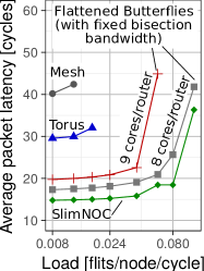
(a) Latency (an adversarial traffic pattern)

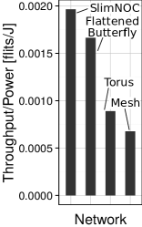
(b) Throughput per power (45nm)

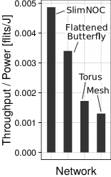
(c) Throughput per power (22nm)

Figure 1. Example advantages of Slim NoC over high- and low-radix NoC topologies (1296 cores); see § 5.1 for detailed methodology. We omit performance data for points after network saturation.

The design of Slim NoC is based on two key observations. First, we observe that SF uses degree-diameter graphs that are challenging to lay out to satisfy NoC constraints such as the same number of routers or nodes on each side of a die. To solve this problem, our key idea is to use non-prime finite fields to generate diameter–2 graphs for SN that fit within these constraints (§ 3.1) and thus can be used to manufacture chips with tens, hundreds, and thousands of cores. Second, we observe that most off-chip topologies optimize cost and layouts in a way that does not address NoC limitations, resulting in large buffers. We solve this problem with NoC-optimized SN layouts and cost models that consider average wire lengths and buffer sizes (§ 3.2). The resulting SN design outperforms state-of-the-art NoC topologies, as our experiments show (§ 5).

To make SN even more scalable and efficient, we augment it with orthogonal state-of-the-art router microarchitecture schemes: central buffer routers (6558397, ) (to decrease buffer area), Elastic Links (4798250, ) and ElastiStore (Seitanidis:2014:EEB:2616606.2616900, ) (to increase performance and power efficiency), and SMART links (Chen:2013:SSR:2485288.2485371, ) (to reduce latency). Doing so leads to a low-diameter and energy-efficient NoC that outperforms other designs, as shown in Figure 1. Example advantages of SN over an FBF, a mesh, and a torus (all using the same microarchitectural schemes as SN) are: (1) latency is lower by $\approx$10%, $\approx$50%, and $\approx$64%, respectively, (2) throughput/power is higher by $\approx$18%, $>$100%, and $>$150% (at 45nm), and $\approx$42%, $>$150%, and $>$250% (at 22nm).

We comprehensively compare SN to five NoC topologies (2D mesh, torus, two Flattened Butterfly variants, and briefly to hierarchical NoCs (yuan2011nonblocking, ; leiserson1985fat, )) using various comparison metrics (area, buffer sizes, static and dynamic power consumption, energy-delay, throughput/power, and performance for synthetic traffic and real applications). We show that SN improves the energy-delay product by $\approx$55% on average (geometric mean) over FBF, the best-performing previous topology, on real applications, while consuming up to $\approx$33% less area. We also analyze SN’s sensitivity to many parameters, such as (1) layout, (2) concentration, (3) router cycle time, (4) network size, (5) technology node, (6) injection rate, (7) wire type, (8) buffer type, (9) bisection bandwidth, (10) router microarchitecture improvement, (11) traffic pattern, and find that SN’s benefits are robust.

Our comprehensive results show that SN outperforms state-of-the-art topologies for both large and small NoC sizes.

2. Background

To alleviate issues of SF for on-chip networks, we first provide background on the SF topology (§ 2.1). We then analyze SF’s performance when used as an on-chip network (§ 2.2).

We broadly introduce the elements and concepts we use in Slim NoC. For the reader’s convenience, we first summarize all symbols in the paper in Table 1.

Network structure	$N$	The number of nodes in the whole network
	$p$	The number of nodes attached to a router (concentration)
	$k^{\prime}$	The number of channels to other routers (network radix)
	$k$	Router radix ($k=k^{\prime}+p$)
	$N_{r}$	The number of routers in the network
	$D$	The diameter of a network
	$q$	A parameter that determines the structure of an SN (see § 2.1)
Physical layout	$M$	The average Manhattan distance between connected routers
	$x_{i}$	$x$ coordinate of a router $i$ ($1\leq i\leq N_{r}$) and its attached nodes
	$y_{i}$	$y$ coordinate of a router $i$ ($1\leq i\leq N_{r}$) and its attached nodes
	$|$VC$|$	The number of virtual channels per physical link
	$[G|a,b]$	A router label in the subgroup view: $G$ is a subgroup type, $a$ is a subgroup ID, $b$ is the position in a subgroup; Figure 2 shows details
	$H$	The number of hops (between routers adjacent to each other on a 2D grid) traversed in one link cycle
Buffer models	$\delta_{ij}$	The size of an edge buffer at a router $i$ connected to $j$ [flits]
	$\delta_{cb}$	The size of a single central router buffer [flits]
	$\Delta_{eb}$	The total size of router buffers in a network with edge buffers [flits]
	$\Delta_{cb}$	The total size of router buffers in a network with central buffers [flits]
	$b$	The bandwidth of a link [bits/s]
	$L$	The size of a flit [bits]
	$T_{ij}$	Round trip time on the link connecting routers $i$ and $j$ [s]
	$W$	The maximal number of wires that can be placed over one router and its attached nodes

Table 1. Symbols used in the paper.

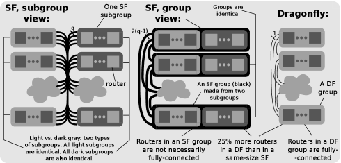
(a) (§ 2.1) A comparison between Slim Fly and Dragonfly (dally08, ).

(b) (§ 3.2) Labeling and indices of Slim Fly routers.

Figure 2. An illustration of the Slim Fly structure and the labeling as well as indices used in the Slim NoC design.

2.1. The Slim Fly Topology: The Main Inspiration

SF (slim-fly, ) is a cost-effective topology for large computing centers that uses mathematical optimization to minimize the network diameter $D$ for a given radix $k$ while maximizing the number of attached nodes $N$ (i.e., network scalability) and maintaining high bandwidth. There are two key reasons for SF’s advantages. First, it lowers diameter ($D=2$): this ensures the lowest latency for many traffic patterns, and it reduces the number of required network resources (packets traverse fewer routers and cables), lowering cost and static/dynamic power consumption (slim-fly, ). Second, it uses graphs that approach the Moore Bound (MB) (mckay98, ), a notion from graph theory that indicates the upper bound on the number of vertices in a graph with a given $D$ and $k$. This maximizes scalability and offers high resilience to link failures because the considered graphs are good expanders (Pippenger:1992:FCN:140901.141867, ).

SF Structure Intuition. SF has a highly symmetric structure; see Figure 2a. It consists of identical groups of routers (see the middle part of Figure 2a). Every two such groups are connected with the same number of cables. Thus, the SF network is isomorphic to a fully-connected graph where each vertex is a collapsed SF group. Still, routers that constitute a group are not necessarily fully-connected. Finally, each group consists of two subgroups of an identical size. These subgroups usually differ in their cabling pattern (slim-fly, ).

SF Structure Details. Routers in SF are grouped into subgroups with the same number of routers (denoted as $q$). There are two types of subgroups, each with the same pattern of intra-group links. Every two subgroups of different types are connected with the same number of cables (also $q$). No links exist between subgroups of the same type. Thus, subgroups form a fully-connected bipartite graph where an edge is formed by $q$ cables. Subgroups of different types can be merged pairwise into identical groups, each with $2q$ routers. Groups form a fully-connected graph where an edge consists of $2(q-1)$ cables. The value of $q$ determines other SF parameters, including the number of routers $N_{r}$, the network radix $k^{\prime}$, the number of nodes $N$, and the concentration $p$.

SF vs. DF. Intuitively, SF is similar to the balanced DF (dally08, ) that also consists of groups of routers. Yet, only one cable connects two DF groups (see Figure 2a), resulting in higher $D$ and a lower number of inter-group links. Moreover, each DF group is a fully-connected graph, which is not necessarily true for SF. Finally, SF reduces the number of routers by $\approx$25% and increases their network radix by $\approx$40% in comparison to a DF with a comparable $N$ (slim-fly, ).

As shown in past work (slim-fly, ), SF maximizes scalability for a fixed $k$ and $D=2$, while maintaining high bandwidth. Other advantages of SN (low cost, power consumption, latency, high resilience) stem from the properties of the underlying degree-diameter graphs. For these, we refer the reader to the original SF work (slim-fly, ).

(a) Wire length

(b) Normalized area

(c) Normalized power

Figure 3. Disadvantages of Slim Fly and Dragonfly used straightforwardly as NoCs (analyses in Figures 3b–3c use 200 cores). i-routers and a-routers are router areas in intermediate and active layers.

2.2. Slim Fly and Dragonfly for On-Chip Networks

We first investigate whether SF or DF can be used straightforwardly as NoCs (see Section 5 for our methodology). We focus on DF and SF as they are the most effective topologies with diameter three and two, respectively (dally08, ; slim-fly, ). They are also direct topologies (each router is attached to equally many cores) and thus easier to manufacture as NoCs. Figure 3 compares SF and DF to a torus (T2D), a concentrated mesh (CM) (balfour2006design, ), and two Flattened Butterflies: a very high-radix full-bandwidth Flattened Butterfly topology (FBF) and an alternative design that has the same bandwidth as the SF topology (PFBF).

Based on Figure 3, we provide two observations. First, compared to PFBF, SF requires $\approx$38% longer wire length, consumes $>$30% more area and power, has $\approx$10% higher latency (not shown), and provides $\approx$35% lower throughput (not shown). Second, we find that DF used on-chip comes with similar overheads. The reasons are as stated in § 1: both SF and DF do not optimize for NoC constraints, use layouts and cost models optimized for rack-level systems, and minimize the use of resources such as bandwidth that are plentiful in NoC settings.

3. Slim NoC Design and Layouts

We first describe the core ideas in SN and how to build it (§ 3.1). Then, we present generic SN models for router placement, sizes of router buffers, and the total cost of a network with a given layout (§ 3.2). We then describe and analyze cost-effective SN layouts (§ 3.3). Finally, we provide detailed mathematical formulations of generating the underlying SN graphs.

3.1. Key Ideas in Slim NoC Construction and Models

Our key idea related to constructing SN is to use non-prime finite fields (slim-fly, ; strang1993introduction, ) to generate the underlying Slim NoC graphs. Specifically, we discover that graphs based on such fields fit various NoC constraints (e.g., die dimensions or numbers of nodes) or reduce wiring complexity. We analyze graphs resulting from non-prime finite fields that enable Slim NoCs with at most 1300 nodes and summarize them in Table 2. The bold and shaded configurations in this table are the most desirable as their number of nodes is a power of two (marked with bold font) or they have equally many groups of routers on each side of a die (marked with grey shades).

The underlying graph of connections in Slim NoC has the same structure based on groups and subgroups as the graph in Slim Fly (see § 2.1). To construct Slim NoC, one first selects (or constructs) a graph that comes with the most desirable configuration (see Table 2). Second, one picks the most advantageous layout based either on the provided analysis (§ 3.3), or one of the proposed particular Slim NoC designs (§ 3.4), or derives one’s own layout using the provided placement, buffer, and cost models (§ 3.2).

	Network radix $k^{\prime}$	Concen- tration $p$	$p=\left\lceil\frac{k^{\prime}}{2}\right\rceil$ ∗	$p/\left\lceil\frac{k^{\prime}}{2}\right\rceil$ ∗∗	Network size $N$	Router count $N_{r}$	Input param. $q$
Non-prime finite fields	6	3	2	66%	64	32	4
	6	3	3	100%	96	32	4
	6	3	4	133%	128	32	4
	12	6	4	66%	512	128	8
	12	6	5	83%	640	128	8
	12	6	6	100%	768	128	8
	12	6	7	116%	896	128	8
	12	6	8	133%	1024	128	8
	13	7	5	71%	810	162	9
	13	7	6	85%	972	162	9
	13	7	7	100%	1134	162	9
	13	7	8	114%	1296	162	9
Prime finite fields	3	2	2	100%	16	8	2
	5	3	2	66%	36	18	3
	5	3	3	100%	54	18	3
	5	3	4	133%	72	18	3
	7	4	3	75%	150	50	5
	7	4	4	100%	200	50	5
	7	4	5	120%	250	50	5
	11	6	4	66%	392	98	7
	11	6	5	83%	490	98	7
	11	6	6	100%	588	98	7
	11	6	7	116%	686	98	7
	11	6	8	133%	784	98	7

Table 2. The configurations of Slim NoC where the network size $N\leq 1300$ nodes. Bold font indicates that in a particular configuration $N$ is a power of two. Grey shade indicates that there are equally many groups on all die sides. Dark grey shade means that, in addition to that, the number of nodes in a given configuration is a square of some integer number. ^∗The ideal concentration, ^∗∗over- or undersubscription.

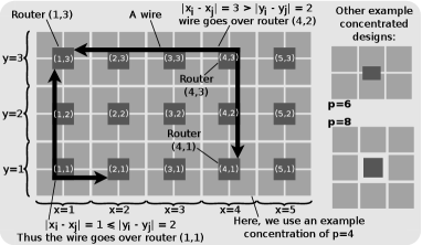
(a) (§ 3.2) The placement model with two example wires.

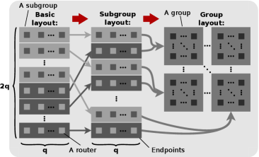
(b) (§ 3.2) Different physical SN layouts.

Figure 4. The details of the SN layout.

3.2. Models

SN reduces diameter to two for low latency. It also minimizes radix $k$ to limit area and power consumption. Yet, when deploying the network on a chip, this may require long multi-cycle links that span a large physical distance. Thus, one needs larger buffers to fully utilize the wire bandwidth, overshadowing the advantages of minimized radix $k$. To alleviate this, we develop new placement, buffer, and cost models for SN (§ 3.2.1–§ 3.2.3) and use them to analyze and compare cost-effective layouts that ultimately minimize the average Manhattan distance and the total buffer area.

3.2.1. Placement Model

When building SN, we place routers on a chip seen as a 2D grid. To analyze different placements, we introduce a model. The model must assign routers their coordinates on a 2D grid, place wires between connected routers, and be easy to use. The model consists of four parts: assigning labels, indices, coordinates, and placing wires.

Labels. We first name each router with a label that uniquely encodes the router position in the SN “subgroup view” (see the leftmost picture in Figure 2a). In this view, any router can be identified using three numbers: (1) type of its subgroup (corresponds to light or dark grey), (2) ID of its subgroup (top-most to bottom-most), and (3) its position in the subgroup (leftmost to rightmost). Labels are based on the subgroup view as its regular structure enables straightforward visualization and identification of routers in any SN. Figure 2b shows the labeling. A router is labeled as $[G|a,b]$. These symbols encode the subgroup type $\left(G\in\{0,1\}\right)$, the subgroup ID $\left(a\in\{1,...,q\}\right)$, and the position in a subgroup $\left(b\in\{1,...,q\}\right)$.

Indices. Second, we translate labels into indices such that each router has a unique index $i\in\{1...N_{r}\}$ based on its label. A formula that ensures uniqueness is $i=Gq^{2}+(a-1)q+b$. Figure 2b shows details. We use indices derived from labels because, while labels are straightforward to construct and use, indices facilitate reasoning about router coordinates on a 2D grid and wire placement.

Coordinates. Indices and labels are used to assign the actual coordinates on a 2D grid; see Figure 4a. A router $i\in\{1...N_{r}\}$ is assigned coordinates $(x_{i},y_{i})$. These coordinates become concrete numbers based on the labels in each layout. More details are in § 3.3. We assume that routers form a rectangle and $1\leq x_{i}\leq X$, $1\leq y_{i}\leq Y$.

Wires. For two connected routers $i$ and $j$, we place the connecting link using the shortest path (i.e., using the Manhattan distance). If the routers lie on the same row or column of the grid, there is only one such path. Otherwise, there are two such paths. We break ties by placing the first wire part (originating at router $i$) vertically (along the Y axis) or horizontally (along the X axis) depending on whether the vertical or horizontal distance is smaller. Formally, we place a wire along the points $(x_{i},y_{i})$, $(x_{i},y_{j})$, and $(x_{j},y_{j})$ (if $|x_{i}-x_{j}|>|y_{i}-y_{j}|$), or $(x_{i},y_{i})$, $(x_{j},y_{i})$, and $(x_{j},y_{j})$ (if $|x_{i}-x_{j}|\leq|y_{i}-y_{j}|$), spreading wires over routers in a balanced way.

The placed wires must adhere to certain placement constraints. We formally describe these constraints for completeness and reproducibility (readers who are not interested in these formal constraints can proceed to § 3.2.2). Specifically, there is a maximum number of wires $W$ that can be placed over a router (and attached nodes). To count wires that traverse a router (and its attached nodes) with given coordinates, we use functions $\Phi$, $\Psi$, $\phi$, and $\psi$. First, for any two routers with indices $i$ and $j$, $\Phi(i,j)$ and $\Psi(i,j)$ determine if the distance between $i$ and $j$ is larger along the X or Y axis, respectively:

(1) $$\Phi(i,j)=1\ \text{if}\ |x_{i}-x_{j}|>|y_{i}-y_{j}|,\ \text{and}\ 0\ \text{otherwise}$$

(2) $$\Psi(i,j)=1\ \text{if}\ |x_{i}-x_{j}|\leq|y_{i}-y_{j}|,\ \text{and}\ 0\ \text{otherwise.}$$

Second, given a router pair $i$ and $j$, $\phi_{ij}(k,l)$ and $\psi_{ij}(k,l)$ determine if a router with coordinates $(k,l)$ is located on one of the two shortest Manhattan paths between $i$ and $j$ ($\phi$ is responsible for the “bottom-left” path as seen in a 2D grid while $\psi$ is responsible for the “top-right” part)

(6) $$\phi_{ij}(k,l)=\left\{\begin{array}[]{l}1,\ \text{if }k=x_{i}\ \wedge\ \text{min}\{y_{i},y_{j}\}\leq l\leq\text{max}\{y_{i},y_{j}\}\\ 1,\ \text{if }l=y_{j}\ \wedge\ \text{min}\{x_{i},x_{j}\}\leq k\leq\text{max}\{x_{i},x_{j}\}\\ 0,\ \text{otherwise}\end{array}\right.$$

(10) $$\psi_{ij}(k,l)=\left\{\begin{array}[]{l}1,\ \text{if }k=x_{j}\ \wedge\ \text{min}\{y_{i},y_{j}\}\leq l\leq\text{max}\{y_{i},y_{j}\}\\ 1,\ \text{if }l=y_{i}\ \wedge\ \text{min}\{x_{i},x_{j}\}\leq k\leq\text{max}\{x_{i},x_{j}\}\\ 0,\ \text{otherwise.}\end{array}\right.$$

To derive the total count of wires crossing a router with coordinates $(k,l)$, we iterate over all pairs of routers and use $\Phi$, $\Psi$, $\phi$, and $\psi$ to determine and count wires that cross $(k,l)$. For a single pair of routers $i$ and $j$, the expression $\phi_{ij}(k,l)\Phi(i,j)+\psi_{ij}(k,l)\Psi(i,j)$ indicates whether the Manhattan path between $i$ and $j$ crosses $(k,l)$ (the first or the second product equals $1$ if the path is “bottom-left” or “top-right”, respectively). Next, we multiply the sum of these products with $\varepsilon_{ij}$: this term determines if routers $i$ and $j$ are connected with a link ($\varepsilon_{ij}=1$) or not ($\varepsilon_{ij}=0$). Finally, for each $(k,l)$, we verify whether its associated wire count is lower than $W$, the maximum value dictated by the technology constraints:

(11) $$\sum_{i=1}^{N_{r}}\sum_{j=1}^{N_{r}}\varepsilon_{ij}[\phi_{ij}(k,l)\Phi(i,j)+\psi_{ij}(k,l)\Psi(i,j)]\leq W$$

Consider two connected routers $A$ and $B$. If $|x_{A}-x_{B}|>|y_{A}-y_{B}|$ then the wire is placed over router/nodes with coordinates $(x_{A},y_{B})$; $\phi_{AB}(k,l)\Phi(A,B)=1$ for any $(k,l)$ contained within line segments connecting points $(x_{A},y_{A})$, $(x_{A},y_{B})$, and $(x_{B},y_{B})$. If $|x_{A}-x_{B}|\leq|y_{A}-y_{B}|$ then the wire is placed over router/nodes with coordinates $(x_{B},y_{A})$; $\psi_{AB}(k,l)\Psi(A,B)=1$ for any $(k,l)$ contained within line segments connecting points $(x_{A},y_{A})$, $(x_{B},y_{A})$, and $(x_{B},y_{B})$.

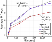
(a) Average wire length $M$.

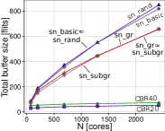
(b) Total size of all buffers in one router (no SMART).

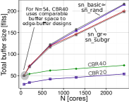
(c) Total size of all buffers in one router (with SMART).

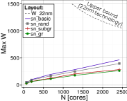
(d) The maximum number of wires placed over a router $W$.

Figure 5. (§ 3.3) The analysis of link lengths and buffer sizes in SN with different layouts ((a)–(c)). The illustration of technological constraints from Eq. (11) (d).

3.2.2. Buffer Size Model

Next, we formally model the size of buffers to provide a tool that enables comparing different Slim NoC layouts in how they reduce the total buffer size.

Edge Buffers. We model the size of an edge buffer integrated with a router $i$ and connected to a wire leading to router $j$ as $\delta_{ij}=\left(T_{ij}b|VC|\right)/L$. This size is proportional to the round trip time (RTT) between $i$ and $j$ ($T_{ij}$), link bandwidth ($b$), and virtual channel count per physical link ($|VC|$). It is inversely proportional to the flit size ($L$). The RTT is $T_{ij}=2\left\lceil(|x_{i}-x_{j}|+|y_{i}-y_{j}|)/{H}\right\rceil+3$ and is proportional to the Manhattan distance between $i$ and $j$. $H$ is the number of hops traversed in one link cycle (a hop is a part of a wire between routers placed next to each other (vertically or horizontally) on a 2D grid). $H$ is $1$ without wire enhancements (such as SMART (Chen:2013:SSR:2485288.2485371, )). We add two cycles for router processing and one cycle for serialization latency.

Lower Latency in Long Wires with SMART Links. SMART (Chen:2013:SSR:2485288.2485371, ) is a technique that builds on driving links asynchronously and placing repeaters carefully to enable single-cycle latency in wires up to 16mm in length at 1GHz at 45nm. For wires that cannot be made single-cycle this way, we assume that SMART can be combined with EB links (4798250, ) to provide multi-cycle wires and full link utilization. We assume SMART has no adverse effect on SN’s error rates as it achieves bit error rates $<10^{-9}$, similarly to links with equivalent full-swing repeaters (Chen:2013:SSR:2485288.2485371, ).

With SMART links, the value of $H$ depends on the technology node and the operational frequency (typically, 8-11 at 1GHz in 45nm) (Chen:2013:SSR:2485288.2485371, ). RTT still grows linearly with wire length; SMART links simply limit the growth rate by a factor of $H$ because a packet can traverse a larger distance on a chip (measured in the distances between neighboring routers) in one cycle. Note that this model may result in edge buffers at different routers having different sizes. To facilitate router manufacturing, one can also use edge buffers of identical sizes. These sizes can be equal to: (1) the minimum edge buffer size in the whole network (reducing $\Delta_{eb}$ but also potentially lowering performance), (2) the maximal edge buffer size in the whole network (increasing $\Delta_{eb}$ but potentially improving throughput), and (3) any tradeoff value between these two.

Central Buffers. We denote the size of a CB as $\delta_{cb}$, this number is a selected constant independent of $|VC|$, $b$, $L$, or $T_{ij}$. CB size is empirically determined by an SN designer.

3.2.3. Cost Model

We now use the layout and buffer models to design the SN cost model. We reduce the average router-router wire length ($M$) and the sum of all buffer sizes in routers ($\Delta_{eb}$ or $\Delta_{cbr}$).

Minimizing Wire Length. The average wire length $M$ is

(12) $$M=\frac{\text{Sum of distances}}{\text{Number of links}}=\frac{\sum_{i=1}^{N_{r}}\sum_{j=1}^{N_{r}}\varepsilon_{ij}(|x_{i}-x_{j}|+|y_{i}-y_{j}|)}{\sum_{i=1}^{N_{r}}\sum_{j=1}^{N_{r}}\varepsilon_{ij}}.$$

To obtain $M$, we divide the sum of the Manhattan distances between all connected routers (the nominator in Eq. (12)) by the number of connected router pairs (the denominator in Eq. (12)). In Eq. (12), we iterate over all possible pairs of routers along both dimensions, and $\varepsilon_{ij}$ determines if routers $i$ and $j$ are connected ($\varepsilon_{ij}=1$) or not ($\varepsilon_{ij}=0$).

Minimizing Sum of Buffer Sizes. One can also directly minimize the total sum of buffer sizes ($\Delta_{eb}$ for an SN with edge buffers and $\Delta_{cb}$ for an SN with central buffers). To derive the size of edge buffers ($\Delta_{eb}$), we sum all the terms $\delta_{ij}$

(13) $$\Delta_{eb}=\sum_{\parbox{28.00006pt}{\centering\scriptsize All router\\ pairs $i,j$\@add@centering}}\parbox{75.0001pt}{\centering\scriptsize If $i,j$ are connected ($\varepsilon_{ij}=1$), add the size of a buffer from $i$ to $j$\\ ($\delta_{ij}=T_{ij}b|VC|/L$)\@add@centering}=\sum_{i=1}^{N_{r}}\sum_{j=1}^{N_{r}}\varepsilon_{ij}\delta_{ij}$$

We calculate the size of the central buffers by a combining the size of the central buffer itself ($\delta_{cb}$) with the size of the staging I/O buffer ($|VC|$ per port). The final sum is independent of wire latencies and the use of SMART links.

(14) $$\Delta_{cb}=\sum_{\parbox{28.00006pt}{\centering\scriptsize All routers\@add@centering}}\parbox{90.00014pt}{\centering\scriptsize Size of a central buffer ($\delta_{cb}$)\\ + Size of I/O staging buffers ($2k^{\prime}|VC|$)\@add@centering}=N_{r}(\delta_{cb}+2k^{\prime}|VC|)$$

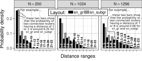
Figure 6. (§ 3.3) Distribution of link distances in SNs. A bar associated with a distance range $X$ illustrates the probability that, for a given layout, two routers are connected with a link that has the distance falling within $X$. Bars of different colors are placed pairwise so that it is easier to compare the subgroup and group layouts.

3.3. Cost-Effective Slim NoC Layouts

We now use the placement, buffer, and cost models from § 3.2 to develop and analyze layouts that minimize the average wire length and the sum of all buffers sizes (see Figure 4b). For each layout, we provide detailed coordinates as a function of router labels $[G|a,b]$ (defined in Table 1 and in § 3.2.1, paragraph “Labels”). We start from the basic layout (sn_basic): subgroups with identical intra-subgroup connections are grouped together and a router $[G|a,b]$ has coordinates $(b,a+Gq)$. As such subgroups are not directly connected, this layout may lengthen inter-subgroup links. To avoid this, the subgroup layout (sn_subgr) mixes subgroups pairwise to shorten wires between subgroups. In this layout, a router $[G|a,b]$ has coordinates $(b,2a-(1-G))$. Both sn_basic and sn_subgr have a rectangular shape ($q\times 2q$ routers) for easy manufacturing. Finally, to reduce the wiring complexity, we use the group layout (sn_gr) where subgroups of different types are merged pairwise and the resulting groups are placed in a shape as close to a square as possible. In sn_gr, there are $q$ groups, each group has identical intra-group connections, and $2(q-1)$ wires connect every two groups. The router coordinates are as follows:

$$x =\left[(a-1)\left\lceil\sqrt{2q}\right\rceil\right]\ \text{mod}\ \left(\left\lceil\sqrt{2q}\right\rceil\left\lceil\sqrt{q}\right\rceil\right)+(b+Gq)\ \text{mod}\ \left\lceil\sqrt{2q}\right\rceil$$

$$y =\left\lfloor\frac{a-1}{\left\lceil\sqrt{q}\right\rceil}\right\rfloor\left\lceil\frac{2q}{\left\lceil\sqrt{2q}\right\rceil}\right\rceil+\left\lceil\frac{b+Gq}{\left\lceil\sqrt{2q}\right\rceil}\right\rceil$$

3.3.1. Evaluating Average Wire Length $M$ and Total Buffer Size $\Delta_{eb}$, $\Delta_{cb}$

We evaluate each layout by calculating $M$, $\Delta_{eb}$, and $\Delta_{cb}$; the results are shown in Figure 5. We also compare to a layout where routers are placed randomly in $q\times 2q$ slots (sn_rand). Figure 5a shows $M$. Both sn_subgr and sn_gr reduce the average wire length by $\approx$25% compared to sn_rand and sn_basic. This reduces $\Delta_{eb}$ as illustrated in Figure 5b; sn_gr reduces $\Delta_{eb}$ by $\approx$18%.

Investigating Details. Figure 6 shows the distribution of wire distances in SNs with $N\in\{200,1024,1296\}$ (these SNs are described in detail in § 3.4) for two best layouts: sn_subgr, sn_gr. The distributions for $N\in\{1024,1296\}$ are similar. We find that sn_gr uses the largest number of the longest links for $N=200$, while sn_subgr uses fewer links traversing the whole die. We use this for designing example ready-to-use Slim NoCs (§ 3.4) that reduce the average wire length the most. We analyze other SNs for $1\leq q\leq 37$: Both sn_gr and sn_subgr consistently reduce the number of the longest wires compared to sn_rand and sn_basic, lowering $M$ and $\Delta_{eb}$ or $\Delta_{cb}$.

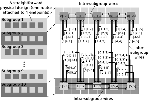
(a) The layout of SN-S, a small-scale SN with $N=200,N_{r}=50$.

(b) The layout of SN-L, a large-scale SN with $N=1296,N_{r}=162$.

Figure 7. (§ 3.4) Example SNs. For clarity, we only show wires connected to two subgroups (in SN-S) and omit inter-group wires (in SN-L).

Adding SMART. With SMART (Chen:2013:SSR:2485288.2485371, ), our sn_subgr and sn_gr layouts reduce $\Delta_{eb}$ by $\approx$10% compared to sn_basic (Figure 5c).

Adding CBRs. We consider small CBs ($\delta_{cb}=20$) and large CBs ($\delta_{cb}=40$). As shown in Figures 5b–5c, CBs result in the lowest total buffer size because the CB size is independent of network radix ($k^{\prime}$) and the round-trip time between routers ($T_{ij}$).

3.3.2. Verifying Constraints

We verify that SN layouts satisfy Eq. (11), i.e., the technological wiring constraints. We assume intermediate metal layers (balfour2006design, ), wiring densities of 3.5k/7k/14k wires/mm, and processing core areas of 4mm² / 1mm² / 0.25mm² at 45nm / 22nm / 11nm (6831831, ). $W$ is the product of the wiring density and the length of a side of a core. We assume that we use a single metal layer (the worst-case scenario); all the remaining available layers can be used by caches and other core components. We present the 45nm analysis in Figure 5d (other technology nodes are similar). No layout violates Eq. (11). We conclude that SN layouts offer advantageous wire length distributions that satisfy the considered technology constraints, enabling feasible manufacturing.

3.3.3. Theoretical Analysis

To formalize SN layouts, we present a brief theoretical analysis.

Bounds: The maximum Manhattan distance between two routers is $q-1$ or $2q-1$ if they are in the same or different subgroups. With this, $M\leq q-1+2q^{4}/N=\sqrt[3]{2N/3}+(\sqrt[3]{4/9})^{2}\sqrt[3]{N}$. Similarly, $\Delta\leq 6Nb(2\sqrt[3]{2N/3}+1)/L$. Thus, $M\in O(\sqrt[3]{N})$ and $\Delta\in O(N\sqrt[3]{N})$. Next, we denote the sum of the lengths of all the intra-group and the inter-group cables as $\mathfrak{L}$ and $\mathfrak{G}$, respectively. One can show that $\mathfrak{L}\geq{3N_{r}q}/{8}$. Then, each router has connections to $q$ other subgroups. The inter-group wires with minimum distances originate in two subgroups containing routers with coordinates $(q,\cdot)$ and $(q+1,\cdot)$ that are in the center of the die. For both subgroups, the minimum possible distances to the connected subgroups are: $1,1,3,3,...,q-2,q-2,q$; using it one can show that $\mathfrak{G}\in\Omega(q^{4})$. We have $M=2{\mathfrak{L}+\mathfrak{G}}/{N_{r}k^{\prime}}\in\Omega(\sqrt[3]{N})$. Similarly, $\Delta\in\Omega(N\sqrt[3]{N})$. Thus: $M\in\Theta(\sqrt[3]{N}),\ \Delta\in\Theta(N\sqrt[3]{N})$.

Theorem 1.

In an SF with $u=0$ and the subgroup layout, $M=\Theta(\sqrt[3]{N})$ and $\Delta=\Theta(N\sqrt[3]{N})$.

(15) $$M \in\Theta(\sqrt[3]{N}),\ \Delta \in\Theta(N\sqrt[3]{N})$$

3.4. Examples of Slim NoC Networks

We now illustrate example SNs that use layouts from § 3 and can be used to manufacture future massively parallel chips.

+	0	1	2	u	v	w	x	y	z
0	0	1	2	u	v	w	x	y	z
1	1	2	0	v	w	u	y	z	x
2	2	0	1	w	u	v	z	x	y
u	u	v	w	x	y	z	0	1	2
v	v	w	u	y	z	x	1	2	0
w	w	u	v	z	x	y	2	0	1
x	x	y	z	0	1	2	u	v	w
y	y	z	x	1	2	0	v	w	u
z	z	x	y	2	0	1	w	u	v

$\times$	0	1	2	u	v	w	x	y	z
0	0	0	0	0	0	0	0	0	0
1	0	1	2	u	v	w	x	y	z
2	0	2	1	x	z	y	u	w	v
u	0	u	x	2	w	z	1	v	y
v	0	v	z	w	x	1	y	2	u
w	0	w	y	z	1	u	v	x	2
x	0	x	u	1	y	v	2	z	w
y	0	y	w	v	2	x	z	u	1
z	0	z	v	y	u	2	w	1	x

$el$	$-el$
0	0
1	2
2	0
u	x
v	z
w	y
x	u
y	w
z	v

+	0	1	u	v	w	x	y	z
0	0	1	u	v	w	x	y	z
1	1	0	v	u	x	w	z	y
u	u	v	0	1	y	z	w	x
v	v	u	1	0	z	y	x	w
w	w	x	y	z	0	1	u	v
x	x	w	z	y	1	0	v	u
y	y	z	w	x	u	v	0	1
z	z	y	x	w	v	u	1	0

$\times$	0	1	u	v	w	x	y	z
0	0	0	0	0	0	0	0	0
1	0	1	u	v	w	x	y	z
u	0	u	w	y	x	z	1	v
v	0	v	y	x	1	u	z	w
w	0	w	x	1	z	v	u	y
x	0	x	z	u	v	y	w	1
y	0	y	1	z	u	w	v	x
z	0	z	v	w	y	1	x	u

$el$	$-el$
0	0
1	1
u	u
v	v
w	w
x	x
y	y
z	z

Table 3. Addition, product, and inverse element tables for an SN based on $\mathbb{F}_{9}$ (three tables on the left) and on $\mathbb{F}_{8}$ (three tables on the right).

A Small Slim NoC for Near-Future Chips. We first sketch an SN design in Figure 7a with $200$ nodes and $50$ routers (denoted as SN-S), targeting the scale of the SW26010 (fu2016sunway, ) manycores that are becoming more common (tile-mx100, ). The input parameter $q=5$ is prime and SN-S is based on a simple finite field $\{0,...,4\}$. SN-S uses concentration $p=4$ and network radix $k^{\prime}=7$, and it consists of 10 subgroups and five groups. Thus, for a rectangular die ($10\times 5$ routers), we use the subgroup layout. This layout also minimizes the number of the longest links traversing the whole chip, cf. Figure 6.

A Large Slim NoC for Future Manycores. The next SN design (denoted as SN-L) addresses future massively parallel chips with $>$1k cores. We use network radix $k^{\prime}=13$ and concentration $p=8$ (one router with its nodes form a square). As the input parameter $q=9=3^{2}$ is a prime power, we use a finite field $\mathbb{F}_{9}$ that cannot be a simple set $\{0,...,8\}$ but must be designed by hand (details are at the end of this section). SN-L has a regular structure with 1296 nodes and 162 routers belonging to 9 identical groups ($18\times 9$ routers). Thus, we use the group layout for easy manufacturing ($3\times 3$ groups) that is illustrated for this particular design in Figure 7b.

A Large Slim NoC with Power-of-Two $N$. We also construct an SN with $1024$ nodes and router radix $12$. Its core count matches the future Adapteva Epiphany (olofsson2016epiphany, ) chip. This SN uses a subgroup layout. Similarly to SN-L, it is based on a prime power $q=8$.

3.5. Generating Slim NoCs: Details

We now provide details on the general algorithm for developing SNs. We first extend the algorithm by Besta and Hoefler (slim-fly, ) (§ 3.5) so that its input is port counts $k^{\prime}$ and $p$, enabling SNs for a selected router design. Then, we snow how to use non-prime finite fields with SN to enable networks that better fit various NoC constraints such as die dimensions or core counts (§ 3.5.2). Finally, we discuss using the number of nodes $N$ as input to construct SNs for a give network size (§ 3.5.3).

3.5.1. Constructing SN for a Fixed Router Radix

We first select router parameters $k^{\prime}$ and $p$ to generate an SN with a desired router design. Here, $k^{\prime}=2w+q$; $w\in\mathbb{N}$ and $q$ is a prime power described in § 2.1 ($q=4w+u$; $u\in\{\pm 1,0\}$). Second, we construct a finite field $\mathbb{F}_{q}$ with $q$ elements. Third, we find an element $\xi\in\mathbb{F}_{q}$ that generates $\mathbb{F}_{q}$: all non-zero elements of $\mathbb{F}_{q}$ can be written as $\xi^{i}$ ($i\in\mathbb{N}$). There is no universal algorithm for finding $\xi$ but a simple exhaustive search can be used. Next, we use $\xi$ to construct two generator sets $X$ and $X^{\prime}$; for $u=1$ we have: $X=\{1,\xi^{2},...,\xi^{q-3}\}$ and $X^{\prime}=\{\xi,\xi^{3},...,\xi^{q-2}\}$. Finally, intra-subgroup and inter-subgroup router connections are established by the following equations (the notation $[G|a,b]\rightleftharpoons[G^{\prime}|a^{\prime},b^{\prime}]$ indicates that routers $[G|a,b]$ and $[G^{\prime}|a^{\prime},b^{\prime}]$ are connected), respectively:

(16) $$\Big{(}[0|a,b]\rightleftharpoons[0|a,b^{\prime}]\Big{)}\Leftrightarrow\Big{(}(b+(-b^{\prime}))\in X\Big{)}$$

(17) $$\Big{(}[1|m,c]\rightleftharpoons[1|m,c^{\prime}]\Big{)}\Leftrightarrow\Big{(}(c+(-c^{\prime}))\in X^{\prime}\Big{)}$$

(18) $$\Big{(}[0|a,b]\rightleftharpoons[1|m,c]\Big{)}\Leftrightarrow\Big{(}b=(m\cdot a+c)\Big{)}$$

3.5.2. Using Non-Prime Finite Fields

Fields $\mathbb{F}_{q}$ based on a prime $q$ are simple: $\mathbb{F}_{q}=\{0,...,q-1\}$; they are used in the original SF. Yet, we discover that graphs based on non-prime $q$ (non-prime finite fields) fit with various NoC constraints (such as die dimensions) or reduce wiring complexity. We analyzed all the graphs resulting from non-prime $q$ with $N<2,000$ and we generated and evaluated the ones that are appropriate candidates for SN. For example, $q=9$ results in a graph with 9 identical groups, facilitating manufacturing.

We build the associated fields by hand. For this, we first define $\mathbb{F}_{q}$ to be a set of arbitrary $q$ elements. Then, we construct addition, product, and inverse element tables: they define the operations on $\mathbb{F}_{q}$ (adding two elements, multiplying two elements, and taking the reverse of an element; all done modulo $q$). Such tables can easily be derived using an exhaustive search. Finally, connections between routers are defined by equations from § 3.5; all the operations in these equations are defined by the respective operation tables.

As an example, for $p=8$ and $k^{\prime}=13$ we have $q=9$. As $q$ is a prime power, there is no finite field $\mathbb{F}_{9}=\{0,...,8\}$ (lidl1997finite, ). Instead, we define $\mathbb{F}_{9}=\{$0,1,2,u,v,w x,y,z$\}$; the symbols are chosen arbitrarily. Then, we construct addition, product, and inverse element tables that define the operations on $\mathbb{F}_{9}$; see Table 3. Next, we calculate $\xi$. There are 4 such (equivalent) elements: v,w,y,z. We then construct $X=\{$1,x,2,u$\}$ and $X^{\prime}=\{$v,y,z,w$\}$ and use them to connect routers.

3.5.3. Constructing SN for a Fixed Network Size

Alternatively, one can also select network size. One first verifies if the selected $N$ is feasible: $N$ must be equal to $N_{r}\cdot p$. Thus, in step 1, a $p$ is selected such that $N=p\cdot N_{r}$ and $N_{r}=2q^{2}$, where $q$ is a prime power as specified in § 2.1 ($N\neq N_{r}\cdot p$ is also feasible by removing some nodes from selected tiles; a strategy used in, e.g, fat trees). Then, in step 2, one verifies the $\kappa$ parameter that determines the tradeoff between node density and contention (see paragraph 3 in § 2.1). If $\kappa$ is acceptable, SN can be developed as described in § 3.5.

4. Slim NoC Microarchitecture

SN provides the lowest radix $k^{\prime}$ for the diameter of two, minimizing buffer area and power consumption while providing low latency. In this section, we further reduce buffer space by extending SN with Central Buffers (CBs) (6558397, ) and optimizing it with ElastiStore (ES) (Seitanidis:2014:EEB:2616606.2616900, ). We first provide background information on CBs and ES (§ 4.1). Then, we show how to combine CBs with virtual channels (VCs) to enable deadlock-freedom (§ 4.2), describe our deadlock-freedom mechanism (§ 4.3), and explain how to maintain full utilization of links when using routers with central buffers (§ 4.4).

4.1. Techniques to Improve Slim NoC Performance

In order to enhance Slim NoC for high performance and low energy consumption, we use two additional mechanisms: Elastic Links and Central Buffer Routers.

Elastic Links: Lower Area and Power Consumption. To reduce the area and power consumption of a NoC, Elastic Buffer (EB) Links (4798250, ; Seitanidis:2014:EEB:2616606.2616900, ) remove input buffers and repeaters within the link pipelines and replace them with master-slave latches. To prevent deadlocks in Slim NoC, we use ElastiStore (ES), which is an extension of EB links (Seitanidis:2014:EEB:2616606.2616900, ). We present design details in § 4.2.

Central Buffer Routers: Less Area. To further reduce area, we use Central Buffer Routers (CBRs) (6558397, ). In a CBR, multi-flit edge (input) buffers are replaced with single-flit input staging buffers and a central buffer (CB) shared by all ports. At low loads, the CB is bypassed, providing a two-cycle router latency. At high loads, in case of a conflict at the output port, a flit passes via the CB, taking four cycles. A CBR employs 3 allocation and 3 traversal stages, which increase the area and power in arbiters and allocators. Yet, it significantly reduces buffer space and thus overall router area and power consumption (6558397, ).

4.2. Combining Virtual Channels with CBs

Original CBs do not support VCs. To alleviate this, we use ElastiStore (ES) links (Seitanidis:2014:EEB:2616606.2616900, ) that enable multiple VCs in the EB channels. The design is presented in Figure 8. ElastiStore links use a separate pipeline buffer and associated control logic for each VC. The per-VC ready-valid handshake signals independently handle the flits of each VC, removing their mutual dependence in the pipelined link. We only keep a slave latch per VC and share the master latch between all VCs. This reduces the overall area and power due to ElastiStore links. The resulting performance loss is minimal and reaches $\frac{1}{|VC|}$ only when all VCs except one are blocked in the pipeline. Other modifications (shown in dark grey) include using per-VC (instead of per-port) I/O staging buffers and CB head/tail pointers to keep VCs independent. The crossbar radix is $k^{\prime}(k^{\prime}+1)$, like in the original CBR. For this, we use a small mux/demux before and after the crossbar inputs and outputs. We maintain single input and output for the CB, which only negligibly impacts performance (6558397, ).

(a)

Figure 8. Modifications to the CB router in § 4.

4.3. Ensuring Deadlock Freedom with CBRs

SN with $D=2$ uses two VCs to avoid deadlocks: VC0 for the first and VC1 for the second hop (assuming paths of lengths up to 2). Here, the only dependency is that of VC0 on VC1, which is not enough to form cycles. We now extend this scheme to the CBR design. To ensure deadlock freedom, two conditions must be met. First, CB allocation for a packet must be atomic: it cannot happen that some flits have entered the CB and the rest are stalled in the links waiting for the CB. Second, head flits of all the packets in different ports and VCs should always be able to compete for the allocation of output ports and VCs. However, since we focus on deterministic routing algorithms, this condition is not required for single deadlock-free deterministic paths.

We satisfy the first condition by reserving the space required for a complete packet during the CB allocation stage. Thus, once a packet takes the CB path, it is guaranteed to move completely into the CB (note that a packet may bypass the CB via the low-load CB bypass path; see § 4.1). A packet in the CB is always treated as a part of the output buffer of the corresponding port and VC. Thus, if the baseline routing is deadlock-free, it remains deadlock-free with the CBR design. Finally, we use SMART links orthogonally to ElastiStore, only to reduce link latency, ensuring no deadlocks. We avoid livelocks with deterministic paths.

4.4. Maintaining Full Link Utilization with CBRs

Large edge buffers enable full utilization of the bandwidth of long wires. For CBR, we obtain the same effect with elastic links (EBs) (Seitanidis:2014:EEB:2616606.2616900, ). Varying the central buffer size reduces head of line blocking.

5. EVALUATION

We evaluate SN versus other topologies in terms of latency, throughput, $\Delta_{cb}$, $\Delta_{eb}$, area, and power consumption.

5.1. Experimental Methodology

Considered Topologies. We compare SN to both low- and high-radix baselines, summarized in Table 4: (1) tori (Alverson:2010:GSI:1901617.1902283, ) (T2D), (2) concentrated meshes (balfour2006design, ) (CM), (3) Flattened Butterflies (dally07, ) (FBF). We also consider SF and DF; their results are consistently worse than others and are excluded for brevity. Note that, for a fixed $N$ and for $D=2$, $k$ and bisection bandwidth of FBF are much higher than those of SN. Thus, for a fair comparison, we develop a partitioned FBF (PFBF) with fewer links to match SN’s $k$ and bisection bandwidth; see Figure 9. We partition an original FBF into smaller identical FBFs connected to one another by one port per node in each dimension. PFBF has $D=4$ while the Manhattan distance between any two routers remains the same as in FBF. Finally, even though we focus on direct topologies, we also briefly compare to indirect hierarchical networks (abeyratne2013scaling, ).

Network	$D$	$N\in\{192,200\}$						$N=1296$
		Sym.	$p$	$k^{\prime}$	$k$	Routers	$N$	Sym.	$p$	$k^{\prime}$	$k$	Routers	$N$
T2D	$\left\lceil\frac{1}{2}\sqrt{N_{r}}\right\rceil$	t2d3	3	4	7	8x8	192	t2d9	9	4	13	12x12	1296
		t2d4	4	4	8	10x5	200	t2d8	8	4	12	18x9	1296
CM	$\left\lceil\sqrt{N_{r}}-2\right\rceil$	cm3	3	4	7	8x8	192	cm9	9	4	13	12x12	1296
		cm4	4	4	8	10x5	200	cm8	8	4	12	18x9	1296
FBF	2	fbf3	3	14	17	8x8	192	fbf9	9	22	31	12x12	1296
		fbf4	4	13	17	10x5	200	fbf8	8	25	33	18x9	1296
PFBF	4	pfbf3	3	8	11	4 FBFs (4x4 each)	192	pfbf9	9	12	21	4 FBFs (6x6 each)	1296
		pfbf4	4	9	13	2 FBFs (5x5 each)	200	pfbf8	8	17	25	2 FBFs (9x9 each)	1296
SN	2	sn_*	4	7	11	10x5	200	sn_*	8	13	21	18x9	1296

Table 4. Considered configurations for two example class sizes.

Figure 9. An example partitioned FBF (1D). Nodes are not shown.

Layouts, Sizes. We compare all the SN layouts from § 3.3 for two size classes: $N\in\{192,200\}$ and $N=1296$. We use both square networks as comparison points that are close in size to SN ($N=192$) and rectangular ones with identical $N$ ($N=200$); see Table 4.

Cycle Times. We use router clock cycle times to account for various crossbar sizes: 0.5ns for SN and PFBF, 0.4ns for topologies with lower radix (T2D, CM), and 0.6ns for high-radix FBF. In specified cases, for analysis purposes, we also use cycle times that are constant across different topologies.

Routing. We focus on static minimum routing where paths between routers are calculated using Dijkstra’s Single Source Shortest Path algorithm (skiena1990dijkstra, ). This is because we aim to design an energy-efficient topology. Adaptive routing would increase overall router complexity and power consumption. Our choice is similar to what is done in many prior works that explored new topologies (4798251, ; xu2009low, ; udipi2010towards, ; kilo-noc, ; hird-journal, ). Moreover, various works that do not introduce new topologies but conduct topology-related evaluations also follow this strategy (aergia, ; das_micro09, ; kim2009low, ).

Yet, it is clear that the routing algorithm can be customized or designed for each topology to maximize performance or energy efficiency and determining the best routing algorithm on a per-topology basis for a given metric is an open research problem. For example, SN can be extended to adaptive routing using paradigms such as the Duato protocol (Dally:2003:PPI:995703, ), UGAL (ugal2005scheme, ), or up-down routing (Dally:2003:PPI:995703, ). We later (§ 6) provide a discussion on adaptive routing in SN. A full exploration of adaptive routing schemes in SN is left for future work.

Wire Architectures. We compare designs with and without SMART links. We use the latency from § 3.2.2 and set the number of hops traversed in one link cycle as $H=9$ (with SMART links) and $H=1$ (no SMART links). We fix the packet size to 6 flits (except for real benchmark traces, see below). All links are 128 bits wide.

Router Architectures. We use routers with central buffers or with edge buffers. An edge router has a standard 2-stage pipeline with two VCs (Peh:2001:DMS:580550.876446, ). The CB router delay is 2 cycles in the bypass path and 4 cycles in the buffered path. Buffer sizes in flits for routers with central buffers are: 1 (input buffer size per VC), 1 (output buffer size per VC), 20 (central buffer size), 20 (injection and ejection queue size). The corresponding sizes for routers without central buffers are, respectively, 5, 1, 0, 20.

Buffering Strategies. EB and CBR prefixes indicate Edge and Central Buffer Routers. We use: EB-Small and EB-Large (all edge buffers have the size of 5 and 15 flits), EB-Var-S and EB-Var-N (edge buffers have minimal possible sizes for 100% link utilization with/without SMART links), CBR-$x$ (CBs of size $x$), and EL-Links (only elastic links).

Synthetic Traffic. We use 5 traffic patterns: random (RND, each source $s$ selects its destination $d$ with uniform random distribution), bit shuffle (SHF, bits in destination ID are shifted by one position), bit reversal (REV, bits in destination ID are reversed), and two adversarial patterns (ADV1 and ADV2; they maximize load on single- and multi-link paths, respectively). We omit the ADV2 results when they are similar to the ADV1 results.

Real Traffic. We use PARSEC/SPLASH benchmark traces to evaluate various real workloads. We run three copies of 64-threaded versions of each benchmark on 192 cores to model a multiprogrammed scenario. We obtain traces for 50M cycles (it corresponds to $\approx$5 billion instructions for SN-S) with the Manifold simulator (wang2014manifold, ), using the DRAMSim2 main memory model (Rosenfeld:2011:DCA:1999163.1999216, ). As threads are spawned one by one, we warm up simulations by waiting for 75% of the cores to be executing. The traces are generated at L1’s back side; messages are read/write/coherence requests. Read requests and coherence messages use 2 flits; write messages use 6 flits (we thus test variable packet sizes). A reply (6 flits) is generated from a destination for each received read request.

Performance Evaluation. We use a cycle-accurate in-house simulator (described by Hassan and Yalamanchili (6558397, ; wang2014manifold, )). Simulations are run for 1M cycles. For $N\in\{192,200\}$ we use detailed topology models (each router and link modeled explicitly). If $N=1296$, due to large memory requirements ($>$40GB), we simplify the models by using average wire lengths and hop counts.

Area and Power Evaluation. We estimate general power consumption using the DSENT tool (dsent, ). We break down area and static power (leakage) due to (1) router-router wires, (2) router-node wires, and (3) actual routers (RR-wires, RN-wires, and routers). We further break down area into global, intermediate, and active layers (denoted as RRg-wires, RRi-wires, and RRa-wires; RNg-wires, RNi-wires, and RNa-wires; g-routers, i-routers, and a-routers, respectively). We break down dynamic power into buffers, crossbars, and wires.

Technologies and Voltages. We use 45nm and 22nm technologies with 1.0V and 0.8V voltages.

We next present a representative subset of our results.

5.2. Analysis of Performance (Latency and Throughput)

We first examine the effects of SN layouts and various buffering strategies on latency and throughput (§ 5.2.1); we next compare SN to other topologies (§ 5.2.2).

5.2.1. Analysis of Layouts and Buffers

Figure 10 shows how the layouts improve the performance of SN. All traffic patterns follow similar trends; we focus on RND. Without SMART links, sn_basic and sn_rand entail higher overheads than sn_subgr and sn_gr due to longer wires. As predicted theoretically (in § 3), sn_subgr and sn_gr are the best for respectively $N=200$ and $N=1296$ in terms of latency and throughput.

(a) Synthetic traffic.

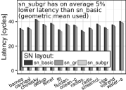
(b) PARSEC/SPLASH.

Figure 10. (§ 5.2.1) Average packet latency with different SN layouts (without SMART links) for synthetic traffic and real applications, for $N=200$.

Figure 11 shows the average packet latency with SN using edge buffers. Without SMART links, small edge buffers lead to higher latency due to high congestion and high overhead of credit-based flow control. EL-Links improve throughput but lead to head-of-line blocking. Both edge buffers and elastic links offer comparable performance to that of central buffers for $N\in\{192,200\}$.

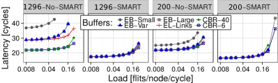
Figure 11. (§ 5.2.1) Impact of buffers (edge buffers, central buffers, no buffers); “200”/“1296” mean $N=200$/$1296$; all variants explained in § 5.1.

We analyze two representative CB sizes (6 and 40 flits) in Figure 11; we also test sizes with 10, 20, 70, and 100 flits. We observe that small CBs outperform (especially for $N>1000$) both edge buffers and EL-Links by removing head-of-line-blocking. Large CBs (e.g., CBR-40) can contain more packets, increasing overall latency.

We also derive the total buffer area for each buffering scheme. we show that SN gives the best tradeoff of radix (hence the crossbar size) for a given diameter and thus it ensures the lowest total buffer size for networks with diameter two, for both edge and central buffer designs.

Impact of SMART Links. SMART links reduce the relative latency differences between Slim NoCs based on different buffering schemes to $\approx$1-3% for most data points, and to up to $\approx$16% for high injection rates that approach the point of network saturation. SMART links accelerate SN by up to $\approx$35% for the sn_subgr layout.

We conclude that: (1) group and subgroup layouts outperform default SN designs, (2) SN with edge buffers can have similar latency and throughput to those of SN designs with elastic links or central buffers, and (3) SN with small CBs has the best performance.

5.2.2. SN versus Other Network Designs

We show that SN outperforms other network designs from Table 4. The results are in Figures 12–13 (SMART links) and 14 (no SMART links). As expected, SN always outperforms CM and T2D. For example, for RND and $N=1296$, SN improves average packet latency by $\approx$45% (over T2D) and $\approx$57% (over CM), and throughput by 10x. This is a direct consequence of SN’s asymptotically lower $D$ and higher bandwidth. SN’s throughput is marginally lower than that of PFBF in some cases (e.g., $N\in\{192,200\}$, REV) because of PFBF’s minimum Manhattan paths. Yet, in most cases SN has a higher throughput than PFBF (e.g., $>$60% for $N=1296$ and RND). SN’s latency is always lower ($\approx$6-25%) than that of PFBF due to its lower $D$. Finally, without SMART links, SN’s longer wires result in higher latency than FBF in several traffic patterns ($\approx$%26 for RND and $N=1296$). In ADV1, SN outperforms FBF (by $\approx$18%). We later (§ 5.4, § 6) show that SN also offers a better power/performance tradeoff than FBF.

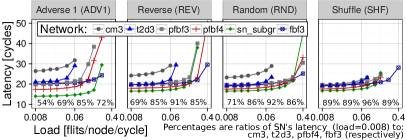
Figure 12. (§ 5.2.2) Performance of synthetic traffic with SMART links for small networks ($N\in\{192,200\}$) and different cycle times for different designs.

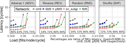
Figure 13. (§ 5.2.2) Performance of synthetic traffic with SMART links for large networks ($N=1296$) and different cycle times for different designs.

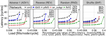
Figure 14. (§ 5.2.2) Performance analysis, $N\in\{192,200\}$, no SMART links.

Impact of SMART Links. SMART links do not impact the latency of CM and T2D as these topologies mostly use single-cycle wires. As expected, SMART links diminish the differences in the performance of different networks with multi-cycle wires.

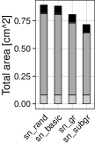
(a) Area of various SN layouts.

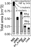
(b) Area of various networks.

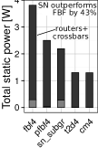
(c) Static power consumption.

Figure 15. Area/power analysis without SMART, $N=200$ (§ 5.3).

5.3. Analysis of Area and Power Consumption

We first briefly analyze area and power differences between various SN layouts. As predicted, sn_subgr outperforms others; for example, see Figure 15a.

Figures 15b–15c present SN’s advantages for $N\in\{192,200\}$ without SMART and central buffers. These are gains from the proposed layouts. SN significantly outperforms FBF in all the evaluated metrics, and PFBF in consumed power. PFBF’s area is smaller; we later use SMART to alleviate this.

Similarly to $N\in\{192,200\}$, SN with $N=1296$ reduces area (by up to $\approx$33%) and power consumption (by up to $\approx$55%) compared to FBF. An exception is pfbf9 as it improves upon SN in both metrics (by $\approx$10-15%). Yet, SN’s higher throughput improves the power/performance tradeoff by $\approx$24% (more details in § 5.4). Thus, SN outperforms FBF (in area and power consumption) and PFBF, CM, and T2D (in power/performance) in designs with $N>1000$.

Impact of SMART Links. Figures 16–17 shows the effect of SMART links on SN. SN reduces area over FBF ($\approx$40-50%) and PFBF ($\approx$9%) as it ensures the lowest $k^{\prime}$ for a given $D$, reducing the area due to fewer buffers and ports as well as smaller crossbars. Low-radix networks deliver the lowest areas but they also entail a worse power/performance tradeoff as shown in § 5.4. Finally, static/dynamic power consumption follows similar trends as the area. For example, SN reduces static power over both FBF ($\approx$45-60%) and PFBF ($\approx$14-27%), as a consequence of providing the lowest $k$ for a given $D$.

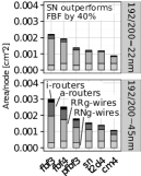
(a) Area.

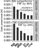
(b) Static power.

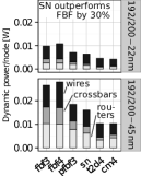
(c) Dynamic power.

Figure 16. (§ 5.3) Area/power analysis with SMART links, $N\in\{192,200\}$.

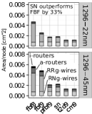
(a) Area.

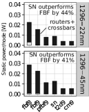
(b) Static power.

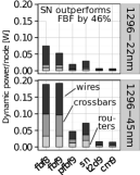
(c) Dynamic power.

Figure 17. (§ 5.3) Area/power analysis with SMART links, $N=1296$.

5.4. Analysis of the Performance–Power Tradeoff

We demonstrate that SN provides the best tradeoff between performance and power out of all the topologies.

Throughput/Power. Table 5 shows SN’s relative improvements over other topologies in the throughput delived per unit of consumed power. To calculate this metric, we divide the number of flits delivered in a cycle by the power consumed during this delivery. SN outperforms all the designs; the lowest gain is over FBF due to its high throughput ($\approx$5-12%) and the highest over low-radix networks ($\geq$50%). Thus, Slim NoC achieves the sweetspot between power consumption and performance (for random traffic).

	$N\in\{192,200\}$					$N=1296$
	t2d4	cm4	pfbf3	fbf3	fbf4	t2d9	cm9	pfbf9	fbf8	fbf9
45nm	96%	97%	17%	12%	6%	155%	235%	38%	54%	52%
22nm	209%	199%	17%	14%	5%	182%	273%	43%	53%	8%

Table 5. (§ 5.4) SN’s advantages in throughput/power (the RND traffic). The percentages are SN’s relative improvements over other topologies in the throughput delived per unit of consumed power. To calculate this metric, we divide the number of flits delivered in a cycle by the power consumed during this delivery.

Energy-Delay. Figure 18 shows the normalized energy-delay product (EDP) results (for PARSEC/SPLASH traces) with respect to FBF. SN reduces EDP by $\approx$55% on average (geometric mean) compared to FBF as it consumes less static and dynamic power. SN’s EDP is also $\approx$29% smaller than that of PFBF due to the latter’s higher latencies and higher power consumption. Similarly, SN reduces EDP by $\approx$19% compared to CM.

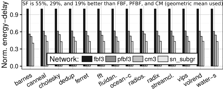
Figure 18. (§ 5.4) Energy-Delay Product analysis (with SMART).

5.5. Further Analysis: A Summary

We summarize our analysis of the influence of other parameters.

Hierarchical NoCs. Although we focus on direct symmetric topologies, we also compare SN to a folded Clos (Scott:2006:BHC:1135775.1136488, ) that represents hierarchical indirect networks such as fat trees or Kilo-core (abeyratne2013scaling, ). SN retains its lower area benefits. For example, its area is $\approx$24% and $\approx$26% smaller for $N=200$ and $N=1296$, respectively.

Other Network Sizes. In addition to $N\in\{200,192,1296\}$, we analyzed other systems where $N\in\{588,686,1024\}$. SN’s advantages are consistent.

Global vs. Intermediate Wires. Both types of wires result in the same advantages of SN over other networks.

Injection Rate. Consumed dynamic power is proportional to injection rates; SN retains its advantages for low and high rates.

45nm vs. 22nm. Both technologies entail similar trends; the only difference is that wires use relatively more area and power in 22nm than in 45nm (see Figures 16–17).

Concentration. SN outperforms other designs for various $p$ ($p\in\{3,4\}$ for $N\in\{192,200\}$ and $p\in\{8,9\}$ for $N\in\{1024,1296\}$).

5.6. Analysis of Today’s Small-Scale Designs

SN specifically targets massively parallel chips. Yet, we also briefly discuss its advantages in today’s small-scale designs ($N=54$), used in, e.g., Intel’s Knights Landing (KNL) (sodani2015knights, ). See Figure 19 for representative results (45nm, SMART). The power/performance tradeoff is similar to that of higher $N$. SN has lower latency than T2D (by $\approx$15%) and PFBF (by $\approx$5%). It uses less power (by $\approx$40%) and area (by $\approx$22%) than FBF and has advantages over PFBF/T2D by $\approx$1-5% in both metrics.

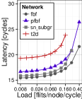
(a) Latency

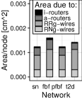
(b) Area

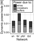
(c) Dynamic power

Figure 19. (§ 5.6) Analysis of small-scale designs (for $N=54$).

Conclusion. Slim NoC retains advantages in small-scale systems where $N$ is small. Slim NoC’s advantages become larger as $N$ grows (cf. § 5). Thus, Slim NoC is likely to become an even more competitive NoC in the foreseeable future.

6. SUMMARY OF RESULTS & DISCUSSION

We now summarize SN’s advantages for $N\in\{192,200\}$ at 45nm. We use the uniform random traffic for illustrating latency and throughput, and PARSEC/SPLASH benchmarks for analyzing EDP.

SN vs. Low-Radix Networks. SN uses more area ($>$27%) and static/dynamic power ($>$40/60%) than T2D and CM, but significantly lowers latency ($>$30%) and increases throughput (3x). Thus, SN improves throughput/power ratio and ED product of selected low-radix designs by $>$95% and $\approx$19%.

SN vs. High-Radix Networks. Compared to FBF, SN has lower bisection bandwidth ($\approx$60%) and has similar latency, but it significantly reduces area ($>$36%), static power ($>$49%), and dynamic power ($>$39%). Thus, it improves the throughput/power ratio ($\approx$5%) and especially EDP ($\approx$55%).

SN vs. Same-Radix Networks. SN delivers a better power/performance tradeoff than PFBF that has comparable bisection bandwidth and radix. SN reduces latency ($\approx$13%), area ($>$9%), static power ($>$25%), and dynamic power ($>$9%), thereby improving throughput/power ($\approx$15%) and EDP ($\approx$15%).

Impact of SMART, CBR. Relative differences between SN and other networks are not vastly affected by SMART/CBR. For example, without SMART, SN uses $\approx$42% less static power than FBF (see Figure 15c), similarly to the difference in static power with SMART (see Figure 16b). We observe (in Table 6) that the average (geometric mean) gain from SMART in the average packet latency of each topology is $\approx$7.6% (FBF), $\approx$0% (CM), $\approx$8% (PFBF), and $\approx$11.3% (SN). We conclude that SN is very synergistic with SMART and CBRs.

	bar.	can.	cho.	de.	fer.	fft	fl.	oc.	radio.	radi.	str.	vip.	vol.	wat.
fbf3	7.7	8.1	6.6	7.3	7.3	8.5	7.3	8.5	9.1	8.2	7.2	8	7.4	6.9
pfbf3	9.2	8.7	6.8	7.5	7.6	9.2	7.3	7.8	9.8	8.6	7.4	8.3	7.6	7.3
cm3	0	0	0	0	0	0	0	0	0	0	0	0	0	0
sn	13.2	11.7	9.8	10.5	10.6	12.6	10.4	10.9	13.6	11.8	10.6	11.6	10.7	10.3

Table 6. (§ 6) Percentage decrease in the average packet latency due to SMART, $N=192$, PARSEC/SPLASH, SN uses sn_subgr.

High-Level Key Observations. Slim NoC achieves a sweetspot in the combined power/performance metrics. It is comparable to or differs negligibly from each compared topology in some metrics (area and power consumption for low-radix and performance (average packet latency, throughput) for high-radix comparison points). It outperforms every other topology in other metrics (performance for low-radix and area as well as power consumption for high-radix topologies). SN outperforms the other networks in combined power/performance metrics, i.e., throughput/power and EDP.

The reasons for SN’s advantages are as stated in § 1. First, it minimizes $k^{\prime}$ (thus reducing buffer space) for fixed $D=2$ (ensuring low latency) and $N$ (enabling high scalability). Next, it uses non-prime finite fields (enabling more configurations). Third, it offers optimized layouts (reducing wire lengths and buffer areas). Finally, it incorporates mechanisms such as SMART or CBR (further reducing buffer areas). We conclude that a combination of all these benefits, enabled by Slim NoC, leads to a highly-efficient and scalable substrate as our evaluations demonstrate.

Adaptive Routing. We conduct a preliminary analysis of adaptive routing. For this analysis, we use the Booksim simulator (jiang2010booksim, ) that provides full support for adaptive routing. Both SN and FBF use simple input-queued routers and do not use any additional mechanisms such as Central Buffers, SMART, or Elastic Links. The simulations use 200 nodes. We analyze SN’s performance with the UGAL protocol (ugal2005scheme, ). We consider two UGAL variants, local (UGAL-L) and global (UGAL-G). In the former, routers can only access the sizes of their local queues. In the latter, routers have access to the sizes of all the queues in the network. We compare SN to FBF that uses two different adaptive schemes (dally07, ): UGAL (a global variant) and an XY adaptive protocol (denoted as XY-ADAPT) that adaptively selects one of available shortest paths (dally07, ). For an additional comparison, we also plot the minimum static routing latency (MIN). Two traffic patterns are used: uniform random and asymmetric, where, for source endpoint $s$, destination $d$ is (with identical probabilities of $\frac{1}{2}$) equal to either $d=(s\mod\frac{N}{2})+\frac{N}{2}$ or $d=(s\mod\frac{N}{2})$. The results are shown in Figure 20. For the uniform random traffic, SN’s UGAL-G and MIN outperform their corresponding schemes in FBF for each injection rate. UGAL-L in SN provides lower (by $\approx$12%) latency for the injection rate of 1%. It is slightly outperformed by FBF’s adaptive schemes for higher loads (by $\approx$1-2%). When the load is very high ($\approx$60%), the protocols in both topologies become comparable. SN offers negligibly higher throughput. For the asymmetric traffic, the performance trends are similar, with the difference that SN’s UGAL schemes have comparable or higher (by $\approx$10%) latency than those of FBF but they provide higher (by $>$100%) throughput. We conclude that, with the UGAL adaptive routing, SN trades latency for higher throughput over FBF with the asymmetric traffic. Under the random traffic, its latency is better than that of FBF under very low ($\approx$1%) injection rates and becomes higher for higher injection rates. Finally, in our evaluation, SN uses a general unoptimized UGAL scheme while FBF incorporates a tuned XY-adaptive scheme. This suggests that developing optimized adaptive routing protocols for SN is a productive area of future research.

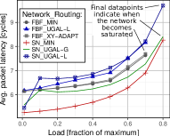
(a) Uniform Random

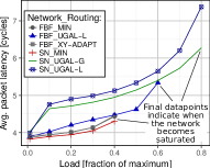
(b) Asymmetric

Figure 20. Preliminary analysis of adaptive routing performance (for $N=200$). Each considered position in a legend has the form “A_B”, where “A” is the network acronym while “B” is the routing scheme acronym. The final data points in each considered combination of network and routing scheme indicate the last evaluated scenario before network saturation.

7. RELATED WORK

To our knowledge, this is the first work to design a highly scalable and energy-efficient on-chip network topology by solving the problems of adapting state-of-the-art off-chip topologies to the on-chip context, using key notions from graph theory and number theory. We discuss how Slim NoC (SN) differs from major related works.

SN vs Slim Fly. SN is inspired by the rack-level Slim Fly (slim-fly, ) (SF) in that it approaches the optimal tradeoff between radix, network size, and diameter by incorporating the underlying MMS graphs (mckay98, ; slim-fly, ). In contrast to SF, SN: (1) uses non-prime finite fields for more viable NoC configurations, (2) provides cost models and layouts suitable for NoC settings, (3) takes advantage of various modern architectural optimizations such as Central Buffers (6558397, ), and (4) resolves deadlock-freedom in NoC settings. Consequently, SN exploits SF’s topological advantages and enables its adaptation to the on-chip constraints for an effective on-chip network design.

SN vs Other NoCs. Other topologies that reduce area and power consumption or maximize performance were proposed, both low-radix (rings (hird-journal, ; hird, ), tori (Alverson:2010:GSI:1901617.1902283, ), meshes (balfour2006design, )) and high-radix (Flattened Butterflies (dally07, ), fully-connected crossbars). Yet, the former have high latency while the latter are power-hungry. The rack-level HyperX (Ahn:2009:HTR:1654059.1654101, ) network extends hypercubes and Flattened Butterfly; it minimizes cost for fixed bisection bandwidth and radix while SN fixes the diameter to two, lowering latency. Indirect networks (Kilo-core (abeyratne2013scaling, ) with swizzle switches (sewell2012swizzle, ), CNoC (kao2011cnoc, ), and hierarchical NoCs (hierarchical, ; hird, ; hird-journal, )) differ from SN, which can be manufactured easier as a direct and symmetric network with identical routers. Various fundamentally low-radix designs (EVCs (express-vc, ), MECS (4798251, ), Kilo-NoC (kilo-noc, ), Dodec (yang2014dodec, ), schemes for 3D networks (xu2009low, ), and others (jain2014high, )) limit throughput at high injection rates; SN ensures a close-to-optimal radix and diameter tradeoff, ensuring low cost and high performance for both low and high loads. Finally, an on-chip Dragonfly topology was only considered in the nanophotonics (pan2009firefly, ) and in-memory processing (ahn2016scalable, ) contexts.

Optimized NoC Buffers. Buffer space can be reduced in many ways (sharing among VCs (damq, ; damq2, ) or ports (dist-shared-buf, ; RoShaq, ; sp2, ), reducing VC count (bubble, ; bcs, ; crit-bubble, ), using bubble flow control (bubble-sharing, ; worm-bubble, ), using scalable networks within switches (Ahn:2008:SHR:2509420.2512433, ), or removing buffers altogether (craik2011investigating, ; bless-rtr, ; chipper, ; fallin2014bufferless, ; nychis2010next, ; nychis2012chip, ; minbd, ; xiang2017carpool, ; xiang2016model, ; cai2015comparative, )). These schemes are largely orthogonal to SN but they may decrease performance at high loads (chipper, ; bless-rtr, ; hat-sbac-pad12, ; nychis2010next, ; nychis2012chip, ; xiang2017carpool, ). Our Elastic Buffer-based Central Buffer routers eliminate the non-determinism and extra link traversals due to deflection-based bufferless routing.

Single-Cycle Wires. ViChaR (nicopoulos2006vichar, ), iDEAL (kodi2008ideal, ), or other schemes for long single-cycle wires (manevich2014designing, ; Chen:2013:SSR:2485288.2485371, ) or deadlock-free multi-VC elastic links (4798250, ; Seitanidis:2014:EEB:2616606.2616900, ) can also enhance SN.

8. CONCLUSION

We introduce Slim NoC (SN), a new family of low-diameter on-chip networks (NoCs) that minimize area and power consumption while providing high performance at both low and high loads. Slim NoC extends the state-of-the-art rack-level Slim Fly topology to the on-chip setting. We identify and preserve Slim Fly’s attractive properties and develop mechanisms to overcome its significant overheads in the NoC setting. In particular, we introduce mathematically rigorous router placement schemes, use non-prime finite fields to generate underlying graphs, thereby producing feasible on-chip layouts, and shift the optimization goal to minimizing radix for a fixed core count. Finally, we augment SN with state-of-the-art mechanisms such as Central Buffer routers, ElastiStore, and SMART links.

We show that Slim NoC can be an effective and feasible on-chip network design for both small-scale and large-scale future chips with tens, hundreds, and thousands of cores. Our evaluations show that Slim NoC significantly improves both performance and energy efficiency for regular and irregular workloads (besta2018log, ; besta2017slimsell, ; tate2014programming, ; schweizer2015evaluating, ) over cutting-edge network topologies. We believe and hope that our approach based on combining mathematical optimization with state-of-the-art engineering will result in other highly-scalable and energy-efficient on-chip network designs.

References

- [1] N. Abeyratne, R. Das, Q. Li, K. Sewell, B. Giridhar, R. G. Dreslinski, D. Blaauw, and T. Mudge. Scaling Towards Kilo-Core Processors with Asymmetric High-Radix Topologies. HPCA, 2013.
- [2] T. Agerwala, J. Martin, J. Mirza, D. Sadler, D. Dias, and M. Snir. SP2 System Architecture. IBM Systems Journal, 1995.
- [3] J. Ahn, S. Hong, S. Yoo, O. Mutlu, and K. Choi. A Scalable Processing-in-Memory Accelerator for Parallel Graph Processing. ISCA, 2015.
- [4] J. H. Ahn, N. Binkert, A. Davis, M. McLaren, and R. S. Schreiber. HyperX: Topology, Routing, and Packaging of Efficient Large-Scale Networks. SC, 2009.
- [5] J. H. Ahn, Y. H. Son, and J. Kim. Scalable High-Radix Router Microarchitecture Using a Network Switch Organization. ACM TACO, 2008.
- [6] R. Alverson, D. Roweth, and L. Kaplan. The Gemini System Interconnect. HOTI, 2010.
- [7] R. Ausavarungnirun, C. Fallin, X. Yu, K. Chang, G. Nazario, R. Das, G. H. Loh, and O. Mutlu. Design and Evaluation of Hierarchical Rings with Deflection Routing. SBAC-PAD, 2014.
- [8] R. Ausavarungnirun, C. Fallin, X. Yu, K. Chang, G. Nazario, R. Das, G. H. Loh, and O. Mutlu. A Case for Hierarchical Rings with Deflection Routing. PARCO, 2016.
- [9] J. Balfour and W. J. Dally. Design Tradeoffs for Tiled CMP On-Chip Networks. ICS, 2006.
- [10] M. Besta and T. Hoefler. Fault tolerance for remote memory access programming models. In Proceedings of the 23rd international symposium on High-performance parallel and distributed computing, pages 37–48, 2014.
- [11] M. Besta and T. Hoefler. Slim Fly: A Cost Effective Low-Diameter Network Topology. SC, 2014.
- [12] M. Besta and T. Hoefler. Accelerating irregular computations with hardware transactional memory and active messages. In Proceedings of the 24th International Symposium on High-Performance Parallel and Distributed Computing, pages 161–172, 2015.
- [13] M. Besta and T. Hoefler. Active access: A mechanism for high-performance distributed data-centric computations. In Proceedings of the 29th ACM on International Conference on Supercomputing, pages 155–164, 2015.
- [14] M. Besta, F. Marending, E. Solomonik, and T. Hoefler. Slimsell: A vectorizable graph representation for breadth-first search. In 2017 IEEE International Parallel and Distributed Processing Symposium (IPDPS), pages 32–41. IEEE, 2017.
- [15] M. Besta, D. Stanojevic, T. Zivic, J. Singh, M. Hoerold, and T. Hoefler. Log (graph) a near-optimal high-performance graph representation. In Proceedings of the 27th International Conference on Parallel Architectures and Compilation Techniques, pages 1–13, 2018.
- [16] Y. Cai, K. Mai, and O. Mutlu. Comparative Evaluation of FPGA and ASIC Implementations of Bufferless and Buffered Routing Algorithms for On-Chip Networks. ISQED, 2015.
- [17] A. Ceyhan, M. Jung, S. Panth, S. K. Lim, and A. Naeemi. Impact of Size Effects in Local Interconnects for Future Technology Nodes: A Study Based on Full-Chip Layouts. IITC/AMC, 2014.
- [18] K. K.-W. Chang, R. Ausavarungnirun, C. Fallin, and O. Mutlu. HAT: Heterogeneous Adaptive Throttling for On-Chip Networks. SBAC-PAD, 2012.
- [19] C.-H. O. Chen, S. Park, T. Krishna, S. Subramanian, A. P. Chandrakasan, and L.-S. Peh. SMART: A Single-Cycle Reconfigurable NoC for SoC Applications. DATE, 2013.
- [20] L. Chen and T. M. Pinkston. Worm-bubble flow control. HPCA, 2013.
- [21] L. Chen, R. Wang, and T. Pinkston. Critical Bubble Scheme: An Efficient Implementation of Globally Aware Network Flow Control. IPDPS, 2011.
- [22] C. Craik and O. Mutlu. Investigating the Viability of Bufferless NoCs in Modern Chip Multi-Processor Systems. CMU Safari Technical Report, 2011.
- [23] W. Dally and B. Towles. Principles and Practices of Interconnection Networks. Morgan Kaufmann Publishers Inc., 2003.
- [24] R. Das, S. Eachempati, A. Mishra, V. Narayanan, and C. Das. Design and Evaluation of a Hierarchical On-Chip Interconnect for Next-Generation CMPs. HPCA, 2009.
- [25] R. Das, O. Mutlu, T. Moscibroda, and C. Das. Application-Aware Prioritization Mechanisms for On-Chip Networks. MICRO, 2009.
- [26] R. Das, O. Mutlu, T. Moscibroda, and C. R. Das. Aérgia: Exploiting Packet Latency Slack in On-Chip Networks. In ISCA, 2010.
- [27] J. J. Dongarra, C. B. Moler, J. R. Bunch, and G. W. Stewart. LINPACK Users’ Guide. SIAM, 1979.
- [28] EZchip Semiconductor Ltd. EZchip Introduces TILE-Mx100 World’s Highest Core-Count ARM Processor Optimized for High-Performance Networking Applications. http://www.tilera.com/News/PressRelease/?ezchip=97, 2015.
- [29] C. Fallin, C. Craik, and O. Mutlu. CHIPPER: A Low-Complexity Bufferless Deflection Router. HPCA, 2011.
- [30] C. Fallin, G. Nazario, X. Yu, K. Chang, R. Ausavarungnirun, and O. Mutlu. MinBD: Minimally-Buffered Deflection Routing for Energy-Efficient Interconnect. NOCS, 2012.
- [31] C. Fallin, G. Nazario, X. Yu, K. Chang, R. Ausavarungnirun, and O. Mutlu. Bufferless and Minimally-Buffered Deflection Routing. Routing Algorithms in Networks-on-Chip, 2014.
- [32] H. Fu, J. Liao, J. Yang, L. Wang, Z. Song, X. Huang, C. Yang, W. Xue, F. Liu, F. Qiao, et al. The Sunway TaihuLight Supercomputer: System and Applications. Science China Information Sciences, 2016.
- [33] R. Gerstenberger, M. Besta, and T. Hoefler. Enabling highly-scalable remote memory access programming with mpi-3 one sided. In Proceedings of the International Conference on High Performance Computing, Networking, Storage and Analysis, pages 1–12, 2013.
- [34] B. Grot, J. Hestness, S. Keckler, and O. Mutlu. Express Cube Topologies for On-Chip Interconnects. HPCA, 2009.
- [35] B. Grot, J. Hestness, S. Keckler, and O. Mutlu. Kilo-NoC: A Heterogeneous Network-on-Chip Architecture for Scalability and Service Guarantees. ISCA, 2011.
- [36] S. Hassan and S. Yalamanchili. Centralized Buffer Router: A Low Latency, Low Power Router for High Radix NoCs. NOCS, 2013.
- [37] S. Hassan and S. Yalamanchili. Bubble Sharing: Area and Energy Efficient Adaptive Routers using Centralized Buffers. NOCS, 2014.
- [38] A. Jain, R. Parikh, and V. Bertacco. High-Radix On-Chip Networks with Low-Radix Routers. ICCAD, 2014.
- [39] N. Jiang, G. Michelogiannakis, D. Becker, B. Towles, and W. J. Dally. Booksim 2.0 User’s Guide. Standford University, 2010.
- [40] Y.-H. Kao, M. Yang, N. S. Artan, and H. J. Chao. CNoC: High-Radix Clos Network-on-Chip. TCAD, 2011.
- [41] J. Kim. Low-Cost Router Microarchitecture for On-Chip Networks. MICRO, 2009.
- [42] J. Kim, W. J. Dally, and D. Abts. Flattened Butterfly: A Cost-Efficient Topology for High-Radix Networks. ISCA, 2007.
- [43] J. Kim, W. J. Dally, S. Scott, and D. Abts. Technology-Driven, Highly-Scalable Dragonfly Topology. ISCA, 2008.
- [44] A. K. Kodi, A. Sarathy, and A. Louri. iDEAL: Inter-Router Dual-Function Energy and Area-Efficient Links for Network-on-Chip (NoC) Architectures. ISCA, 2008.
- [45] A. Kumar, L.-S. Peh, P. Kundu, and N. Jha. Toward Ideal On-Chip Communication Using Express Virtual Channels. IEEE Micro, 2008.
- [46] C. E. Leiserson. Fat-Trees: Universal Networks for Hardware-Efficient Supercomputing. IEEE TC, 1985.
- [47] R. Lidl and H. Niederreiter. Finite Fields: Encyclopedia of Mathematics and Its Applications. Comp. & Math. with Applications, 33(7):136–136, 1997.
- [48] J. Liu and J. G. Delgado-Frias. A DAMQ Shared Buffer Scheme for Network-on-Chip. CSS, 2007.
- [49] R. Manevich, L. Polishuk, I. Cidon, and A. Kolodny. Designing Single-Cycle Long Links in Hierarchical NoCs. Microprocessors and Microsystems, 2014.
- [50] B. D. McKay, M. Miller, and J. Širán. A Note on Large Graphs of Diameter Two and Given Maximum Degree. Journal of Combinatorial Theory, Series B, 1998.
- [51] G. Michelogiannakis, J. Balfour, and W. Dally. Elastic-Buffer Flow Control for On-Chip Networks. HPCA, 2009.
- [52] T. Moscibroda and O. Mutlu. A Case for Bufferless Routing in On-Chip Networks. ISCA, 2009.
- [53] C. Nicopoulos, D. Park, J. Kim, N. Vijaykrishnan, M. S. Yousif, and C. R. Das. ViChaR: A Dynamic Virtual Channel Regulator for Network-on-Chip Routers. MICRO, 2006.
- [54] G. Nychis, C. Fallin, T. Moscibroda, and O. Mutlu. Next Generation On-Chip Networks: What Kind of Congestion Control Do We Need? In HotNets, 2010.
- [55] G. P. Nychis, C. Fallin, T. Moscibroda, O. Mutlu, and S. Seshan. On-Chip Networks from a Networking Perspective: Congestion and Scalability in Many-Core Interconnects. SIGCOMM, 2012.
- [56] A. Olofsson. Epiphany-V: A 1024 Processor 64-bit RISC System-on-Chip. arXiv preprint arXiv:1610.01832, 2016.
- [57] Y. Pan, P. Kumar, J. Kim, G. Memik, Y. Zhang, and A. Choudhary. Firefly: Illuminating Future Network-on-Chip with Nanophotonics. ISCA, 2009.
- [58] L.-S. Peh and W. J. Dally. A Delay Model and Speculative Architecture for Pipelined Routers. HPCA, 2001.
- [59] Pezy Computing. PEZY-SC2. http://pezy.jp.
- [60] N. Pippenger and G. Lin. Fault-Tolerant Circuit-Switching Networks. SPAA, 1992.
- [61] V. Puente, R. Beivide, J. Gregorio, J. Prellezo, J. Duato, and C. Izu. Adaptive Bubble Router: A Design to Improve Performance in Torus Networks. ICPP, 1999.
- [62] R. Ramanujam, V. Soteriou, B. Lin, and L.-S. Peh. Design of a High-Throughput Distributed Shared-Buffer NoC Router. NOCS, 2010.
- [63] P. Rosenfeld, E. Cooper-Balis, and B. Jacob. DRAMSim2: A Cycle Accurate Memory System Simulator. IEEE CAL, 2011.
- [64] P. Schmid, M. Besta, and T. Hoefler. High-performance distributed rma locks. In Proceedings of the 25th ACM International Symposium on High-Performance Parallel and Distributed Computing, pages 19–30, 2016.
- [65] H. Schweizer, M. Besta, and T. Hoefler. Evaluating the cost of atomic operations on modern architectures. In 2015 International Conference on Parallel Architecture and Compilation (PACT), pages 445–456. IEEE, 2015.
- [66] S. Scott, D. Abts, J. Kim, and W. J. Dally. The BlackWidow High-Radix Clos Network. ISCA, 2006.
- [67] I. Seitanidis, A. Psarras, G. Dimitrakopoulos, and C. Nicopoulos. ElastiStore: An Elastic Buffer Architecture for Network-on-Chip Routers. DATE, 2014.
- [68] K. Sewell, R. G. Dreslinski, T. Manville, S. Satpathy, N. Pinckney, G. Blake, M. Cieslak, R. Das, T. F. Wenisch, D. Sylvester, D. Blaauw, and T. Mudge. Swizzle-Switch Networks for Many-Core Systems. Emerging and Selected Topics in Circuits and Systems, 2012.
- [69] A. Singh. Load-Balanced Routing in Interconnection Networks. PhD thesis, Stanford University, 2005.
- [70] S. Skiena. Dijkstra’s algorithm. Implementing Discrete Mathematics: Combinatorics and Graph Theory with Mathematica. Addison-Wesley, 1990.
- [71] A. Sodani. Knights Landing (KNL): 2nd Generation Intel® Xeon Phi Processor. HCS, 2015.
- [72] E. Solomonik, M. Besta, F. Vella, and T. Hoefler. Scaling betweenness centrality using communication-efficient sparse matrix multiplication. In Proceedings of the International Conference for High Performance Computing, Networking, Storage and Analysis, pages 1–14, 2017.
- [73] G. Strang. Introduction to Linear Algebra. Wellesley-Cambridge Press Wellesley, MA, 1993.
- [74] C. Sun, C. O. Chen, G. Kurian, L. Wei, J. E. Miller, A. Agarwal, L. Peh, and V. Stojanovic. DSENT - A Tool Connecting Emerging Photonics with Electronics for Opto-Electronic Networks-on-Chip Modeling. NOCS, 2012.
- [75] Y. Tamir and G. Frazier. Dynamically-Allocated Multi-Queue Buffers for VLSI Communication Switches. IEEE TC, 1992.
- [76] A. Tate, A. Kamil, A. Dubey, A. Größlinger, B. Chamberlain, B. Goglin, C. Edwards, C. J. Newburn, D. Padua, D. Unat, et al. Programming abstractions for data locality. 2014.
- [77] A. T. Tran and B. M. Baas. RoShaQ: High-Performance On-Chip Router with Shared Queues. ICCD, 2011.
- [78] A. N. Udipi, N. Muralimanohar, and R. Balasubramonian. Towards Scalable, Energy-Efficient, Bus-Based On-Chip Networks. HPCA, 2010.
- [79] J. Wang, J. Beu, R. Bheda, T. Conte, Z. Dong, C. Kersey, M. Rasquinha, G. Riley, W. Song, H. Xiao, P. Xu, and S. Yalamanchili. Manifold: A Parallel Simulation Framework for Multicore Systems. ISPASS, 2014.
- [80] R. Wang, L. Chen, and T. M. Pinkston. Bubble Coloring: Avoiding Routing- and Protocol-Induced Deadlocks with Minimal Virtual Channel Requirement. ICS, 2013.
- [81] X. Xiang, S. Ghose, O. Mutlu, and N.-F. Tzeng. A Model for Application Slowdown Estimation in On-Chip Networks and Its Use for Improving System Fairness and Performance. ICCD, 2016.
- [82] X. Xiang, W. Shi, S. Ghose, L. Peng, O. Mutlu, and N.-F. Tzeng. Carpool: A Bufferless On-Chip Network Supporting Adaptive Multicast and Hotspot Alleviation. ICS, 2017.
- [83] Y. Xu, Y. Du, B. Zhao, X. Zhou, Y. Zhang, and J. Yang. A Low-Radix and Low-Diameter 3D Interconnection Network Design. HPCA, 2009.
- [84] H. Yang, J. Tripathi, N. E. Jerger, and D. Gibson. Dodec: Random-Link, Low-Radix On-Chip Networks. MICRO, 2014.
- [85] X. Yuan. On Nonblocking Folded-Clos Networks in Computer Communication Environments. IPDPS, 2011.