Quasinormal modes and self-adjoint extensions of the Schroedinger operator

Abstract

We revisit here the analytical continuation approach usually employed to compute quasinormal modes (QNM) and frequencies of a given potential barrier $V$ starting from the bounded states and respective eigenvalues of the Schroedinger operator associated with the potential well corresponding to the inverted potential $-V$. We consider an exactly soluble problem corresponding to a potential barrier of the Poschl-Teller type with a well defined and behaved QNM spectrum, but for which the associated Schroedinger operator $\cal H$ obtained by analytical continuation fails to be self-adjoint. Although $\cal H$ admits self-adjoint extensions, we show that the eigenstates corresponding to the analytically continued QNM do not belong to any self-adjoint extension domain and, consequently, they cannot be interpreted as authentic quantum mechanical bounded states. Our result challenges the practical use of the this type of method when $\cal H$ fails to be self-adjoint since, in such cases, we would not have in advance any reasonable criterion to choose the initial eigenstates of $\cal H$ which would correspond to the analytically continued QNM.

I Introduction

Usually, the quasinormal mode (QNM) analysis [1, 2] consists in looking for solutions of the form $\Psi(t,x)=e^{-i\omega t}u(x)$ of an $(1+1)$-dimensional wave equation, with $u(x)$ obeying a Schroedinger-like equation

$$\left(-\epsilon^{2}\frac{d^{2}}{dx^{2}}+V(x)\right)u=\omega^{2}u,$$ (1)

on a certain domain of $\mathbb{R}$, with $\epsilon$ standing for some intrinsic scale parameter of the problem. Typically, as for instance in the problems involving asymptotically flat black-hole situations [1, 2], the modes $u$ are defined on the entire real line $\mathbb{R}$, which is usually assumed to be spanned by a tortoise-coordinate $x$, and $V(x)$ is a positive potential barrier, vanishing sufficiently fast when approaching the horizon ($x\to-\infty$) and the spatial infinity $(x\to\infty)$. The QNM frequencies are the complex values of $\omega$ such that the solutions of (1) behave as outgoing waves at infinity and ingoing ones at the horizon, which, according to our definition for $\Psi$, correspond, respectively, to solutions such that $u\propto e^{\frac{i\omega x}{\epsilon}}$ for $x\to\infty$ and $u\propto e^{-\frac{i\omega x}{\epsilon}}$ for $x\to-\infty$. Also according to our definition, the modes will be exponentially suppressed in time, and consequently could be interpreted as asymptotically stable perturbations, if $\Im\omega<0$.

There are several strategies to solve a QNM problem in pratice, see [1, 2] for comprehensive reviews on this vast issue. The analytical continuation method, introduced decades ago with the pioneering works of Blome, Ferrari, and Mashhoon [3, 4, 5], is one of the best options to have analytical answers and gain some physical insights on the problem. This method consists basically in a formal map between the QNM solutions of (1) and the bounded states of the quantum mechanical problem corresponding to the case of the inverted potential barrier $-V(x)$, which would be governed by the Schroedinger operator

$${\cal H}=-\hbar^{2}\frac{d^{2}}{dx^{2}}-V(x).$$ (2)

We know that for $V(x)$ vanishing sufficiently fast, the bounded states of $\cal H$ will decay exponentially, i.e., $\psi\propto e^{\mp\sqrt{-E}\frac{x}{\hbar}}$ for $x\to\pm\infty$, with ${\cal H}\psi=E\psi$. We will adopt here the analytical continuation prescription introduced recently by Hatsuda [6], which is based in the key observation that, taking formally $\hbar=i\epsilon$ in (2), one can map the quantum mechanical bound states of $\cal H$ in the QNM of (1) with frequencies formally given by

$$\omega^{2}=-E(\hbar=i\epsilon).$$ (3)

The converse path is also possible, and we will indeed explore it here. Starting with the QNM modes of a potential barrier, one can obtain the associated bounded states for the inverted potential Schroedinger operator $\cal H$ by formally setting $\epsilon=-i\hbar$ in (1) and reversing (3). Although this construction is not entirely rigorous and, in particular, we cannot assure that all pertinent solutions of the problem may be found by the analytical continuation in the parameters $\epsilon$ and $\hbar$, the obtained solutions are certainly valid ones as we can check by direct calculations.

This kind of analytical continuation approach has proved to be rather efficient and, in fact, it has been used for a vast range of QNM analysis recently. In the present paper, we unveil a potential pitfall when the Schroedinger operator $\mathcal{H}$ fails to be self-adjoint, which is a rather common situation, for instance, when the problem is restricted to the half real line $\mathbb{R}_{+}$, see [7, 8, 9, 10] for further references on this kind of problem. We will exhibit an explicit example of a problem on $\mathbb{R}_{+}$ with a well defined and behaved QNM spectrum, but for which the associated Schroedinger operator $\mathcal{H}$ obtained by the analytical continuation $\epsilon=-i\hbar$ fails to be self-adjoint. Moreover, we show that, although $\mathcal{H}$ admits self-adjoint extensions, the eigenstates corresponding to the analytically continued QNM are not in the domain of any self-adjoint extension of $\mathcal{H}$ and, consequently, they cannot be interpreted as authentic quantum mechanical bounded states. This means that, if we had chosen to solve this problem starting with the quantum mechanical analytically continued $\mathcal{H}$, we would not have any hint or practical prescription to choose the initial eigenstates of $\cal H$ which would correspond to the analytically continued QNM. Practically, we would not succeed in applying the analytical continuation method for this kind of problem.

II The QNM problem

We will be concerned here with a specific case where the domain of the QNM is the half real line $\mathbb{R}_{+}$. This could correspond, for instance, to the case of naked singularities [11, 12], but certainly there will be other similar cases in distinct situations, see, for instance, [13, 14] for examples involving asymptotically AdS spacetimes. We will consider specifically the infinite potential barrier on $\mathbb{R}_{+}$ given by

$$V(x)=\frac{V_{0}}{\sinh^{2}x}+\frac{V_{1}}{\cosh^{2}x},$$ (4)

where $V_{0}>0$ and $x\in(0,\infty)$, which is known to be exactly integrable since the seminal works of Poschl and Teller, see for instance [13, 14] and the references therein.

We know, on physical grounds, that the QNM modes associated the potential (4) should correspond to solutions of (1) obeying the boundary conditions $u(0)=0$ (infinite impenetrable barrier) and $u\propto e^{i\omega x}$ for $x\to\infty$ (outgoing wave in the spatial infinity). We will follow [13] closely and introduce the variable $z\in(0,1]$ such that $z=1/\cosh^{2}x$, in terms of which equation (1) reads

$$z(1-z)u^{\prime\prime}-\left(1-\frac{3}{2}z\right)u^{\prime}+\frac{1}{4}\left(\frac{\omega^{2}}{z}-\frac{V_{0}}{1-z}-{V_{1}}\right)u=0,$$ (5)

where the tilde denotes derivation with respect to $z$. Equation (5) can be easily solved in terms of hypergeometric functions and its general solution can be written as combination of the functions [13]

$$u=z^{\alpha}(1-z)^{\beta}{}_{2}F_{1}\left(a,b;c;z\right),$$ (6)

where

$$a = \alpha+\beta+\gamma_{+},$$ (7)

$$b = \alpha+\beta+\gamma_{-},$$ (8)

$$c = 2\alpha+1,$$ (9)

$$\alpha = \pm\frac{i\omega}{2},$$ (10)

$$\beta = \frac{1}{4}\left(1\pm\sqrt{1+4V_{0}}\right),$$ (11)

$$\gamma_{\pm} = \frac{1}{4}\left(1\pm\sqrt{1-4V_{1}}\right).$$ (12)

The general solution of the second order linear differential equation (5) involves two linearly independent functions which can be written as a combination of the possible choices of $\alpha$ and $\beta$ according to (10) and (11). However, notice that in the spatial infinity limit $x\to\infty$ ($z\to 0^{+}$), one has $u=z^{\alpha}=e^{\mp i\omega x}$ for any choice of $\beta$. Moreover, as one can see from the Wronskian in the spatial infinity limit, the functions $u$ corresponding to the two possible choices for $\alpha$ are linearly independent regardless the value chosen for $\beta$. Hence, we can choose without loss of generality the positive sign for $\beta$ for the general solution of (5). However, the solution (6) is obtained under the condition of $c\notin\mathbb{Z}$, in fact, the case with $c$ an integer positive or negative will explore later on.

The boundary condition of an outgoing wave at spatial infinity $z\to 0^{+}$ requires to select only the $\alpha=-\frac{i\omega}{2}$ mode in the general solution. On the other hand, the $x\to 0^{+}$ limit corresponds to $z\to 1^{-}$, and thus in order to impose the second QNM boundary condition $\lim_{x\to 0^{+}}u=0$, we need to determine the behavior of our solution for $z\to 1^{-}$. By exploring the well known identity 15.3.6 of [15],

$${}_{2}F_{1}\left(a,b;c;z\right) = \frac{\Gamma(c)\Gamma(c-a-b)}{\Gamma(c-a)\Gamma(c-b)}{}_{2}F_{1}\left(a,b;a+b-c+1;1-z\right)$$

$$+\frac{\Gamma(c)\Gamma(a+b-c)}{\Gamma(a)\Gamma(b)}(1-z)^{c-a-b}{}_{2}F_{1}\left(c-a,c-b;c-a-b+1;1-z\right),$$

and that $z=1-x^{2}+{\cal O}(x^{4})$ for $x\to 0^{+}$, we have the following behavior for $u(x)$ near $x=0$

$$u=Ax^{2\beta}\left(1+{\cal O}(x^{2})\right)+Bx^{1-2\beta}\left(1+{\cal O}(x^{2})\right),$$ (14)

where

$$A=\frac{\Gamma(1-i\omega)\Gamma\left(\frac{1}{2}-2\beta\right)}{\Gamma\left(1-\beta-\gamma_{+}-\frac{i\omega}{2}\right)\Gamma\left(1-\beta-\gamma_{-}-\frac{i\omega}{2}\right)}$$ (15)

and

$$B=\frac{\Gamma(1-i\omega)\Gamma\left(2\beta-\frac{1}{2}\right)}{\Gamma\left(\beta+\gamma_{+}-\frac{i\omega}{2}\right)\Gamma\left(\beta+\gamma_{-}-\frac{i\omega}{2}\right)}.$$ (16)

Since $\beta>\frac{1}{2}$, the second term in (14) is always singular for $x\to 0^{+}$, but it can be indeed removed by exploring the $\Gamma$-function poles in (16). Explicitly, we will have $\lim_{x\to 0^{+}}u=0$ if the QNM frequencies $\omega$ are such that

$$\omega_{\pm}=-i\left(2n+1+\sqrt{V_{0}+\frac{1}{4}}\pm\sqrt{\frac{1}{4}-V_{1}}\right),$$ (17)

with $n\in\mathbb{Z}_{\geq 0}$ This result coincides with the pertinent limit of the calculations presented in [13]. Notice that, with the choice (17) for the frequencies, the coefficient $A$ given by (15) reads

$$A_{\pm}=\frac{\left(-1-\sqrt{V_{0}+\frac{1}{4}}\right)_{n}}{\left(-(n+1)-\sqrt{V_{0}+\frac{1}{4}}\mp\sqrt{\frac{1}{4}-V_{1}}\right)_{n}},$$ (18)

where $(\ )_{n}$ stands for the usual falling factorial function

$$(x-1)_{n}=\frac{\Gamma(x)}{\Gamma(x-n)}.$$ (19)

Also, one can see from (14) that the QNM are solutions $u(x)$ such that

$$\frac{u(x)}{\sqrt{x}}=Ax^{\delta}\left(1+{\cal O}(x^{2})\right),$$ (20)

and

$$\sqrt{x}u^{\prime}(x)=\left(\frac{1}{2}+\delta\right)Ax^{\delta}\left(1+{\cal O}(x^{2})\right),$$ (21)

with the prime now denoting differentiation with respect to $x$, $A$ given by (18), and

$$\delta=\sqrt{\frac{1}{4}+V_{0}}.$$ (22)

Finally, we have that the QNM are solutions $u(x)$ for which

$$\lim_{x\to 0^{+}}x^{-\delta}\left(\sqrt{x}u^{\prime}(x)-\frac{1}{\sqrt{x}}\left(\frac{1}{2}+\delta\right)u(x)\right)=0.$$ (23)

This expression for the effective boundary condition obeyed by the QNM at $x=0$ will be important in the self-adjointness analysis of $\mathcal{H}$ in the next section.

It is worth mentioning that the simple exact spectrum (17) illustrates clearly all qualitative behaviors that QNM can exhibit. First, reminding that $V_{0}>0$, we see that for $V_{1}>\frac{1}{4}$, the QNM frequencies will have the well known form

$$\omega=\sqrt{V_{1}-\frac{1}{4}}-i\left(2n+1+\sqrt{V_{0}+\frac{1}{4}}\right),$$ (24)

denoting that the associated QNM are the usual exponentially suppressed oscillatory modes. On the other hand, for $V_{1}\leq\frac{1}{4}$, we have the so-called algebraically special QNM, for which the associated frequencies are purely imaginary quantities. Notice that if $V_{1}$ is small enough, one could effectively attain regimes with $\Im\omega_{-}>0$, denouncing the presence of exponentially amplified modes. We will return to this point in the last section, but we can advance that these unstable modes are related to the existence of a region with $V(x)<0$ for negative $V_{1}$.

If $c=\ell\in\mathbb{Z}_{\geq 1}$ then the second solution of the hypergeometric equation contains a logaritmic branch [15]. The latter term is discarded provided it blows up as $z\rightarrow 1^{-}$, that is, one has to deal with only one solution given by the following expression:

$$u_{2}=z^{\alpha}(1-z)^{\beta}{}_{2}F_{1}\left(a,b,\ell;z\right),$$ (25)

where this solution ensures the condition of having an out-going wave at infinity as long as $\alpha=\alpha_{-}$. One has to inspect the behavior of (25) near $x\rightarrow 0$ to see whether or not $u_{2}$ vanishes. Making use of (II) and (14) one concludes that the coefficients in (14) are similar to (15) and (16) but now the specific condition $c=\ell\in\mathbb{Z}_{\geq 1}$ must be enforced. The term propotional to $x^{2\beta}$ goes to zero and the Gamma function $\Gamma(1-i\omega)$ is well-behaved provided $\ell$ is not a negative integer. However, the second term in (14) diverges for $2\beta>1$ then it is mandatory that the coefficient $B$ must goes to zero. The latter possiblity is reached when $2(\beta+\gamma_{\pm})-i\omega=-2n$ with $n\in\mathbb{Z}_{\geq 0}$, which agrees with (17) and with the resul reported in [13] about the QNMs for pure De Sitter in the massless limit. Notice also that the spectrum (17) corresponds to the poles of the $\Gamma$-functions in the denominator of the coefficient $B$ in (16) and, hence, we are assuming that the respective numerator is regular in these points. Although this is always the case when $V_{1}>\frac{1}{4}$, we can have situations with algebraically special modes for which the numerators have exactly the same poles of the denominators. This is the case, for instance, of $c=1-i\omega_{\pm}$ being zero or a negative integer, which implies that the second solution of the hypergeometric equation admits a logaritmic bran ch and one has to get rid of it [15], yielding to

$$u_{3}=z^{-\alpha}(1-z)^{\beta}{}_{2}F_{1}\left(a-c+1,b-c+1,2-c;z\right),$$ (26)

where one selects $\alpha=\alpha_{+}$ to reproduce the right behavior at infinity, $u_{3}\propto e^{+i\omega x}$. As one would expect the condition $c=1-i\omega_{\pm}\in\mathbb{Z}_{\leq 0}$ has somekind of impact in the QNMs. In order to see that more clearly, it is convenient to assume that $V_{0}=\mu(\mu+1)$ and $V_{1}=\nu(1-\nu)$. Applying the same identity (II) for the hypergeometric function ${}_{2}F_{1}\left(a-c+1,b-c+1,2-c;z\right)$ with the new coefficients, one can read off the QNM spectrum and show that it reduces to

$$\omega_{+} = -i(2n+1+\mu+\nu),$$ (27)

$$\omega_{-} = -i(2n+1+\mu-(\nu-1)),$$ (28)

with $n\in\mathbb{Z}_{\geq 0}$. Once again, the previous analysis is consistent with the one reported in [13]. Eqns. (27-28) tell us that whenever $\mu\pm\nu$ is a positive integer, the poles of $\Gamma(2-c)=\Gamma(1-i\omega)$ coincide with those ones in the denominators of $u_{3}(x)$ when the hypergeometric function ${}_{2}F_{1}\left(a-c+1,b-c+1,2-c;z\right)$ is re-written with the help of (II), and consequently we cannot enforce the boundary condition $\lim_{x\to 0^{+}}u_{3}=0$ without having trivially $u_{3}(x)=0$. There are no QNMs in this case, and such a behavior is a remnant of the curious phenomenon of the so-called reflectionless eigenstates for the Poschl-Teller potentials in Quantum Mechanics, see [16].

We finish mentioning that, since $\beta>\frac{1}{2}$, the QNM limit $u\propto x^{2\beta}$ for $x\to 0^{+}$ assures that the energy integral

$${\cal E}=\int\left[(\partial_{t}\Psi)^{2}+(\partial_{x}\Psi)^{2}+V(x)\Psi^{2}\right]dx$$ (29)

always converges for $x\to 0^{+}$, confirming that the QNM are rather well behaved for the potential barrier (4).

III The quantum mechanical problem

We will address now the following problem: would it be possible to obtain the QNM of the last section by means of an analytical continuation approach as described in Section I? As we will see, the answer is no, at least in the usual sense of associating QNM and bounded states of the Schroedinger operator (2) by an analytical continuation in the parameters $\epsilon$ and $\hbar$. The equivalent quantum mechanical problem can be formulated by means of the formal map $\epsilon=-i\hbar$ of the first section. Notice that the parameter $\epsilon$ is a “hidden” scale in the QNM problem, we have absorbed it in our calculations so far with the tacit rescalings $V\leftrightarrow V/\epsilon^{2}$ and $\omega\leftrightarrow\omega/\epsilon$. Assuming also $\hbar=1$, we have that the the analytical continuation will map the QNM $u$ of the potential barrier in eigenstates $\psi$ of the potential well corresponding to the inverted potential barrier according to

$$\psi=u\left(V\to-V,\omega\to-i\omega\right).$$ (30)

The associated eigenvalues (energies) will be given by

$$E=\omega^{2}\left(V\to-V\right),$$ (31)

and from (17) we have

$$E_{\pm}=-\left(2n+1+\sqrt{\frac{1}{4}-V_{0}}\pm\sqrt{\frac{1}{4}+V_{1}}\right)^{2}.$$ (32)

Such expression for the energy shows that, in contrast with the QNM analysis of the potential barrier, now we have necessarily to deal with two qualitatively distinct cases accordingly with the attractiveness of the inverted potential at $x\to 0^{+}$: $0<V_{0}\leq\frac{1}{4}$ and $V_{0}>\frac{1}{4}$. This is hardly a surprise, this class of behavior for an attractive $1/x^{2}$ potential is well known in the literature, see [8, 9] for instance. Moreover, since one can have complex values of $E$ for $V_{0}>\frac{1}{4}$ or $V_{1}<\frac{1}{4}$, the self-adjointness of $\cal H$ is clearly an issue here.

The self-adjointness analysis of a Schroedinger operators $\cal H$ always starts [7, 8, 9, 10] with the deficiency indexes $n_{+}$ and $n_{-}$, which stand here for the respective dimensions of the so-called deficiency subspaces $N_{\pm}\subset D({\mathcal{H}^{\dagger}})$ defined by

$$N_{\pm}=\left\{\phi\in D({\mathcal{H}^{\dagger}}),\quad{\mathcal{H}}\phi=\pm i\phi\right\},$$ (33)

where ${\mathcal{H}^{\dagger}}$ is the adjoint of ${\mathcal{H}}$ and $D({\mathcal{H}^{\dagger}})\subset L^{2}[0,\infty)$ stands for its domain. The deficiency subspaces $N_{\pm}$ can be constructed directly form the formulas of the previous section. For instance, in order to determine $N_{+}$, one needs to consider the case $\omega^{2}=i$, leading to two linearly independent solutions which behavior at spatial infinity will be $\phi_{\pm}\propto e^{\pm i\left(\frac{1+i}{\sqrt{2}}\right)x}$. However, only $\phi_{+}$ is square integrable, and hence we have just concluded that $n_{+}\leq 1$. Furthermore, we have also from the results of Section II that, for $x\to 0^{+}$,

$$\phi_{+}=\sqrt{x}\left(A_{+}x^{\delta}+B_{+}x^{-\delta}\right),$$ (34)

with $\delta$ given by the substitution $V_{0}\to-V_{0}$ in (22) and $A_{+}$ and $B_{+}$ obtained by setting $\omega=\frac{1+i}{\sqrt{2}}$ in the expressions (15) and (16), respectively. Notice that (34) is square integrable for $x\to 0^{+}$ and no other restriction is necessary on $\phi_{+}$. We have just established that $n_{+}=1$. Since similar results hold for $N_{-}$, we have that ${\mathcal{H}}$ is not self-adjoint, but the von Neumann formulas [9] assure that ${\mathcal{H}}$ admits a one-parameter family of self-adjoint extensions. In order to construct such extensions, we need the the function $\phi_{-}$, i.e., the square integrable solution for ${\mathcal{H}}\phi=-i\phi$. Its behavior for $x\to 0^{+}$ is

$$\phi_{-}=\sqrt{x}\left(A_{-}x^{\delta}+B_{-}x^{-\delta}\right),$$ (35)

with the constants $A_{-}$ and $B_{-}$ defined as in (34), but now for $\omega=\frac{i-1}{\sqrt{2}}$. The self-adjoint extensions of $\mathcal{H}$ are determined by the boundary conditions on $\psi\in D({\mathcal{H}^{\dagger}})$ such that

$$\left\langle\phi,\mathcal{H}\psi\right\rangle-\left\langle\mathcal{H}\phi,\psi\right\rangle=\lim_{x\to 0^{+}}[\bar{\phi}(x)\psi^{\prime}(x)-{\bar{\phi}}^{\prime}(x)\psi(x)]=0,$$ (36)

where the inner product is the usual $L^{2}[0,\infty)$ product and $\phi$ is a linear combination of $\phi_{+}$ and $\phi_{-}$, which we write without loss of generality as

$$\phi=\phi_{+}+\bar{\lambda}\phi_{-},$$ (37)

where $\lambda$ is a free complex parameter. From (36), we have that the self-adjoint extensions of $\mathcal{H}$ will be given by the following boundary conditions on the eingenstates $\psi$

$$\lim_{x\to 0^{+}}\left(\sqrt{x}\left[\mathcal{A}_{\lambda}x^{\bar{\delta}}+\mathcal{B}_{\lambda}x^{-\bar{\delta}}\right]\psi^{\prime}(x)-\frac{1}{\sqrt{x}}\left[\left(\frac{1}{2}+\bar{\delta}\right)\mathcal{A}_{\lambda}x^{\bar{\delta}}+\left(\frac{1}{2}-\bar{\delta}\right)\mathcal{B}_{\lambda}x^{-\bar{\delta}}\right]\psi(x)\right)=0,$$ (38)

where

$$\mathcal{A}_{\lambda}=\bar{A}_{+}+\lambda\bar{A}_{-}$$ (39)

and

$$\mathcal{B}_{\lambda}=\bar{B}_{+}+\lambda\bar{B}_{-}.$$ (40)

For each value of the free parameter $\lambda$, we have a distinct self-adjoint extension of the Schroedinger operator $\mathcal{H}$ characterized by the boundary condition (38) at $x=0$. Notice that (38) coincides wit the usual self-adjoint boundary condition of $1/x^{2}$ attractive potentials, the so-called Calogero problem, see [8, 9].

Now, let us consider the QNM boundary condition (23), which the analytically continued eigenstates would also be expected to obey in the quantum mechanical problem. We have two qualitatively distinct cases. Let us consider first the case of real nonzero $\delta$, i.e., $0<V_{0}<\frac{1}{4}$. The QNM boundary condition requires a value for $\lambda$ such that $\mathcal{A}_{\lambda}=0$ in order to select the $x^{-\delta}$ terms in (38). However, in this case one has

$$\lim_{x\to 0^{+}}x^{-\delta}\left(\sqrt{x}u^{\prime}(x)-\frac{1}{\sqrt{x}}\left(\frac{1}{2}-\delta\right)u(x)\right)=0,$$ (41)

which clearly does not coincide with (23), meaning that no self-adjoint extension of $\mathcal{H}$ can accommodate the QNM boundary condition for the case of real nonzero $\delta$. The so-called critical case $\delta=0$ could be analyzed in a similar way, but in this case the deficiency subspaces $N_{\pm}$ are generated by the solutions

$$\phi_{\pm}=\sqrt{x}\left(A_{\pm}+B_{\pm}\ln x\right),$$ (42)

see [8, 9] for further details on this particular case of the $1/x^{2}$ potential. The situation for imaginary $\delta$ is analogous. We need to have $\mathcal{B}_{\lambda}=0$, to select the $x^{\bar{\delta}}$ terms, but we will end up with (41) once more, implying again that no self-adjoint extension of $\mathcal{H}$ will be able to accommodate the QNM boundary condition for the case of imaginary $\delta$ as well.

In summary, although $\mathcal{H}$ fails to be self-adjoint in the quantum mechanical problem corresponding to the inverted potential (4), it admits self-adjoint extensions. However, the eigenstates corresponding to the analytically continued QNM are not in the domain of any self-adjoint extension of $\mathcal{H}$ and, consequently, they cannot be interpreted as authentic quantum mechanical bounded states. In particular, they can fail to have real eigenvalues, see (32), and to be square-integrable.

IV Final remarks

Let us return to the unstable algebraically special modes presented in (17) for negative $V_{1}$. Although the behavior of the potential barrier (4) depends only on $V_{0}$ for $x\to 0^{+}$, the situation for $x\to\infty$ is clear different, since we have

$$V(x)=\frac{4(V_{0}+V_{1})}{e^{2x}}\left(1+\mathcal{O}(e^{-2x})\right)$$ (43)

in this limit. As one can see, for $V_{0}+V_{1}<0$, the potential $V$ approaches zero for $x\to\infty$ from below and, hence, it must have a minimum somewhere in $\mathbb{R}^{+}$. It is indeed easy to locate this minimum, it corresponds to the point $x=x^{*}$ such that

$$\tanh^{4}x^{*}=-\frac{V_{0}}{V_{1}},$$ (44)

for which we have simply

$$V(x^{*})=-\left(\sqrt{V_{0}}-\sqrt{-V_{1}}\right)^{2},$$ (45)

remembering that $V_{0}>0$ and $V_{1}<-V_{0}$. Fig. 1 illustrates a typical

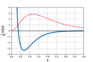
Figure 1: Illustration of an unstable algebraically special QNM. Solid blue line: Potential barrier (4) for $V_{0}/V_{1}=-\frac{1}{8}$. Red traced line: the unstable mode (no scale) corresponding to the $n=0$ case in the frequency $\omega_{-}$ in (17).

unstable algebraically special QNM. The curious observation is that the unstable QNM with a purely imaginary QNM frequency (17) corresponds, in fact, to a bounded state of the potential barrier! The deficiency indexes for the Schroedinger operator associated with the original potential (4) are $n_{+}=n_{-}=0$ since no solution of $\mathcal{H}u=\pm iu$ is square integrable, implying that $\mathcal{H}$ for the case of a repulsive potential is self-adjoint and, in particular, it may admit bounded states as that one depicted in Fig. 1.

V summary

We have shown that the QNM solutions $u$ of the potential barrier $V$ given by (4) can be analytically continued in eigenstates $\psi$ of the Schroedinger operator $\mathcal{H}$ associated with the inverted potential $-V$. However, the eigenstates $\psi$ are not in the domain of any self-adjoint extension of $\mathcal{H}$, challenging the practical use of the analytical continuation method for this kind of potential barrier. If we had tried to solve this problem starting with the states of $\mathcal{H}$, we would not have any physical or mathematical criterion to select the states $\psi$ which would given origin to the QNM $u$ via the analytical continuation. Furthermore, if we have tried starting with a genuine quantum state of $\mathcal{H}$, after the analytical continuation we would get a solution of the QNM problem which does not obey the correct boundary conditions. In other words, this result poses a serious challenge on how to extend the analytic continuation method in several spacetimes (naked singularity, pure De sitter, etc) to obtain the proper QNMs. Whether the analytic continuation approach can be applied to other more complex scenarios or not is something that deserves to be explored in the future. For instance, one may wonder about its applicability in the case of a Dirac field propagating on those backgrounds [13],[17]. The so-called PT-symmetric extensions of the Schroedinger operator (see, for instance, [18] and references therein) and the pseudospectrum of non-selfadjoint operators [19] are also interesting points to be explored in the context of our QNM analysis.

- [1] E. Berti, V. Cardoso, and A.O. Starinets, Class. Quantum Grav. 26, 163001 (2009), [arXiv:0905.2975]
- [2] R.A. Konoplya and A. Zhidenko, Rev. Mod. Phys. 83, 793 (2011), [arXiv:1102.4014].
- [3] H. J. Blome and B. Mashhoon, Phys. Lett. 110A, 231 (1984).
- [4] V. Ferrari and B. Mashhoon, Phys. Rev. Lett. 52, 1361 (1984).
- [5] V. Ferrari and B. Mashhoon, Phys. Rev. D 30, 295 (1984).
- [6] Y. Hatsuda, Phys. Rev. D 101, 024008 (2020).
- [7] G. Bonneau, J. Faraut, and G. Valent, Am. J. Phys. 69, 322 (2001). [arXiv:quant-ph/0103153]
- [8] A.M. Essin and D.J. Griffiths, Am. J. Phys. 74, 109 (2006).
- [9] D.M. Gitman, I.V. Tyutin, and B.L. Voronov, Self-adjoint Extensions in Quantum Mechanics: General Theory and Applications to Schrödinger and Dirac Equations with Singular Potentials, Birkhäuser (2012).
- [10] A. P. Balachandran, A. R. de Queiroz, and A. Saa, Near-horizon modes and self-adjoint extensions of the Schroedinger operator, in Classical and Quantum Physics 60 Years Alberto Ibort Fest Geometry, Dynamics, and Control, Eds. G. Marmo, D. Martin de Diego, and M. Muñoz Lecanda, Springer Proceedings in Physics book series (SPPHY, volume 229), 2019. [arXiv:1810.00020].
- [11] C. Chirenti, A. Saa, and J. Skakala, Phys. Rev. D 86, 124008 (2012). [arXiv:1206.0037]
- [12] C. Chirenti, A. Saa, and J. Skakala, Phys. Rev. D 87, 044034 (2013). [arXiv:1211.1046]
- [13] D.P. Du, B. Wang, and R.K. Su, Phys. Rev. D 70, 064024 (2004). [arXiv:hep-th/0404047]
- [14] A.F. Cardona and C. Molina, Class. Quantum Grav. 44 245002 (2017).
- [15] M. Abramowitz and I. Stegun, Handbook of Mathematical Functions: with Formulas, Graphs, and Mathematical Tables, Dover Publications (1965).
- [16] J. Lekner, Am. J. Phy. 75, 1151 (2007).
- [17] M. Casals, S. R. Dolan, B. C. Nolan, A. C. Ottewill, E. Winstanley. Kermions: quantization of fermions on Kerr space-time. Phys.Rev.D 87 064027 (2013).
- [18] C.M. Bender, D.C. Brody, and H.F. Jones, Phys. Rev. Lett. 89, 270401 (2002). [arXiv:quant-ph/0208076]
- [19] J.L. Jaramillo, R.P. Macedo, and L. Sheikh, Pseudospectrum and black hole quasi-normal mode (in)stability, [arXiv:2004.06434]