Iterative Amortized Policy Optimization

Abstract

Policy networks are a central feature of deep reinforcement learning (RL) algorithms for continuous control, enabling the estimation and sampling of high-value actions. From the variational inference perspective on RL, policy networks, when used with entropy or KL regularization, are a form of amortized optimization, optimizing network parameters rather than the policy distributions directly. However, direct amortized mappings can yield suboptimal policy estimates and restricted distributions, limiting performance and exploration. Given this perspective, we consider the more flexible class of iterative amortized optimizers. We demonstrate that the resulting technique, iterative amortized policy optimization, yields performance improvements over direct amortization on benchmark continuous control tasks. Accompanying code: github.com/joelouismarino/variational_rl.

1 Introduction

Reinforcement learning (RL) algorithms involve policy evaluation and policy optimization [73]. Given a policy, one can estimate the value for each state or state-action pair following that policy, and given a value estimate, one can improve the policy to maximize the value. This latter procedure, policy optimization, can be challenging in continuous control due to instability and poor asymptotic performance. In deep RL, where policies over continuous actions are often parameterized by deep networks, such issues are typically tackled using regularization from previous policies [67, 68] or by maximizing policy entropy [57, 23]. These techniques can be interpreted as variational inference [51], using optimization to infer a policy that yields high expected return while satisfying prior policy constraints. This smooths the optimization landscape, improving stability and performance [3].

However, one subtlety arises: when used with entropy or KL regularization, policy networks perform amortized optimization [26]. That is, rather than optimizing the action distribution, e.g., mean and variance, many deep RL algorithms, such as soft actor-critic (SAC) [31, 32], instead optimize a network to output these parameters, learning to optimize the policy. Typically, this is implemented as a direct mapping from states to action distribution parameters. While such direct amortization schemes have improved the efficiency of variational inference as “encoder” networks [44, 64, 56], they also suffer from several drawbacks: 1) they tend to provide suboptimal estimates [20, 43, 55], yielding a so-called “amortization gap” in performance [20], 2) they are restricted to a single estimate [27], thereby limiting exploration, and 3) they cannot generalize to new objectives, unlike, e.g., gradient-based [36] or gradient-free optimizers [66].

Inspired by techniques and improvements from variational inference, we investigate iterative amortized policy optimization. Iterative amortization [55] uses gradients or errors to iteratively update the parameters of a distribution. Unlike direct amortization, which receives gradients only after outputting the distribution, iterative amortization uses these gradients online, thereby learning to iteratively optimize. In generative modeling settings, iterative amortization empirically outperforms direct amortization [55, 54] and can find multiple modes of the optimization landscape [27].

The contributions of this paper are as follows:

• We propose iterative amortized policy optimization, exploiting a new, fruitful connection between amortized variational inference and policy optimization.

• Using the suite of MuJoCo environments [78, 12], we demonstrate performance improvements over direct amortized policies, as well as more complex flow-based policies.

• We demonstrate novel benefits of this amortization technique: improved accuracy, providing multiple policy estimates, and generalizing to new objectives.

2 Background

2.1 Preliminaries

We consider Markov decision processes (MDPs), where $\mathbf{s}_{t}\in{\mathcal{S}}$ and $\mathbf{a}_{t}\in{\mathcal{A}}$ are the state and action at time $t$, resulting in reward $r_{t}=r(\mathbf{s}_{t},\mathbf{a}_{t})$. Environment state transitions are given by $\mathbf{s}_{t+1}\sim p_{\textrm{env}}(\mathbf{s}_{t+1}|\mathbf{s}_{t},\mathbf{a}_{t})$, and the agent is defined by a parametric distribution, $p_{\theta}(\mathbf{a}_{t}|\mathbf{s}_{t})$, with parameters $\theta$. The discounted sum of rewards is denoted as $\mathcal{R}(\tau)=\sum_{t}\gamma^{t}r_{t}$, where $\gamma\in(0,1]$ is the discount factor, and $\tau=(\mathbf{s}_{1},\mathbf{a}_{1},\dots)$ is a trajectory. The distribution over trajectories is:

$$p(\tau)=\rho(\mathbf{s}_{1})\prod_{t=1}^{T-1}p_{\textrm{env}}(\mathbf{s}_{t+1}|\mathbf{s}_{t},\mathbf{a}_{t})p_{\theta}(\mathbf{a}_{t}|\mathbf{s}_{t}),$$ (1)

where the initial state is drawn from the distribution $\rho(\mathbf{s}_{1})$. The standard RL objective consists of maximizing the expected discounted return, $\mathbb{E}_{p(\tau)}\left[{\mathcal{R}}(\tau)\right]$. For convenience of presentation, we use the undiscounted setting ($\gamma=1$), though the formulation can be applied with any valid $\gamma$.

2.2 KL-Regularized Reinforcement Learning

Various works have formulated RL, planning, and control problems in terms of probabilistic inference [21, 8, 79, 77, 11, 51]. These approaches consider the agent-environment interaction as a graphical model, then convert reward maximization into maximum marginal likelihood estimation, learning and inferring a policy that results in maximal reward. This conversion is accomplished by introducing one or more binary observed variables [19], denoted as $\mathcal{O}$ for “optimality” [51], with

$$p(\mathcal{O}=1|\tau)\propto\exp\big{(}\mathcal{R}(\tau)/\alpha\big{)},$$

where $\alpha$ is a temperature hyper-parameter. We would like to infer latent variables, $\tau$, and learn parameters, $\theta$, that yield the maximum log-likelihood of optimality, i.e., $\log p(\mathcal{O}=1)$. Evaluating this likelihood requires marginalizing the joint distribution, $p(\mathcal{O}=1)=\int p(\tau,\mathcal{O}=1)d\tau$. This involves averaging over all trajectories, which is intractable in high-dimensional spaces. Instead, we can use variational inference to lower bound this objective, introducing a structured approximate posterior distribution:

$$\pi(\tau|\mathcal{O})=\rho(\mathbf{s}_{1})\prod_{t=1}^{T-1}p_{\textrm{env}}(\mathbf{s}_{t+1}|\mathbf{s}_{t},\mathbf{a}_{t})\pi(\mathbf{a}_{t}|\mathbf{s}_{t},\mathcal{O}).$$ (2)

This provides the following lower bound on the objective:

$$\log p(\mathcal{O}=1) =\log\int p(\mathcal{O}=1|\tau)p(\tau)d\tau$$ (3)

$$\geq\int\pi(\tau|\mathcal{O})\bigg{[}\log\frac{p(\mathcal{O}=1|\tau)p(\tau)}{\pi(\tau|\mathcal{O})}\bigg{]}d\tau$$ (4)

$$=\mathbb{E}_{\pi}[\mathcal{R}(\tau)/\alpha]-D_{\mathrm{KL}}(\pi(\tau|\mathcal{O})\|p(\tau)).$$ (5)

Equivalently, we can multiply by $\alpha$, defining the variational RL objective as:

$$\mathcal{J}(\pi,\theta)\equiv\mathbb{E}_{\pi}[\mathcal{R}(\tau)]-\alpha D_{\mathrm{KL}}(\pi(\tau|\mathcal{O})\|p(\tau)).$$ (6)

This objective consists of the expected return (i.e., the standard RL objective) and a KL divergence between $\pi(\tau|\mathcal{O})$ and $p(\tau)$. In terms of states and actions, this objective is:

$$\mathcal{J}(\pi,\theta)=\mathbb{E}_{\begin{subarray}{c}\mathbf{s}_{t},r_{t}\sim p_{\textrm{env}}\\ \mathbf{a}_{t}\sim\pi\end{subarray}}\left[\sum_{t=1}^{T}r_{t}-\alpha\log\frac{\pi(\mathbf{a}_{t}|\mathbf{s}_{t},\mathcal{O})}{p_{\theta}(\mathbf{a}_{t}|\mathbf{s}_{t})}\right].$$ (7)

At a given timestep, $t$, one can optimize this objective by estimating the future terms in the sum using a “soft” action-value ($Q_{\pi}$) network [30] or model [62]. For instance, sampling $\mathbf{s}_{t}\sim p_{\textrm{env}}$, slightly abusing notation, we can write the objective at time $t$ as:

$$\mathcal{J}(\pi,\theta)=\mathbb{E}_{\pi}\left[Q_{\pi}(\mathbf{s}_{t},\mathbf{a}_{t})\right]-\alpha D_{\mathrm{KL}}(\pi(\mathbf{a}_{t}|\mathbf{s}_{t},\mathcal{O})||p_{\theta}(\mathbf{a}_{t}|\mathbf{s}_{t})).$$ (8)

Policy optimization in the KL-regularized setting corresponds to maximizing $\mathcal{J}$ w.r.t. $\pi$. We often consider parametric policies, in which $\pi$ is defined by distribution parameters, $\bm{\lambda}$, e.g., Gaussian mean, $\bm{\mu}$, and variance, $\bm{\sigma}^{2}$. In this case, policy optimization corresponds to maximizing:

$$\bm{\lambda}\leftarrow\textrm{arg}\max_{\bm{\lambda}}\mathcal{J}(\pi,\theta).$$ (9)

Optionally, we can then also learn the policy prior parameters, $\theta$ [1].

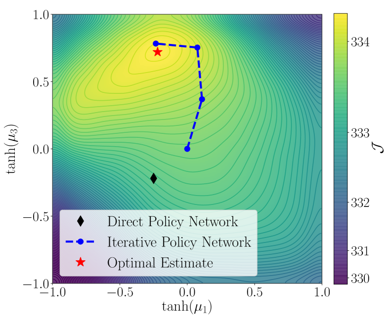
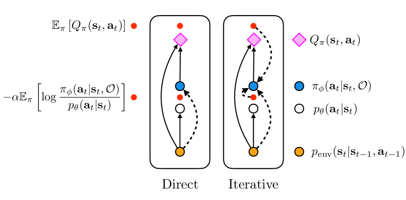
Figure 1: Amortization. Left: Optimization over two dimension of the policy mean, $\mu_{1}$ and $\mu_{3}$, for a particular state. A direct amortized policy network outputs a suboptimal estimate, yielding an amortization gap in performance. An iterative amortized policy network finds an improved estimate. Right: Diagrams of direct and iterative amortization. Larger circles denote distributions, and smaller red circles denote terms in the objective, $\mathcal{J}$ (Eq. 8). Dashed arrows denote amortization. Iterative amortization uses gradient feedback during optimization, while direct amortization does not.

2.3 Entropy & KL Regularized Policy Networks Perform Direct Amortization

Policy-based approaches to RL typically do not directly optimize the action distribution parameters, e.g., through gradient-based optimization. Instead, the action distribution parameters are output by a function approximator (deep network), $f_{\phi}$, which is trained using deterministic [70, 52] or stochastic gradients [83, 35]. When combined with entropy or KL regularization, this policy network is a form of amortized optimization [26], learning to estimate policies. Again, denoting the action distribution parameters, e.g., mean and variance, as $\bm{\lambda}$, for a given state, $\mathbf{s}$, we can express this direct mapping as

$$\bm{\lambda}\leftarrow f_{\phi}(\mathbf{s}),$$ (direct amortization) (10)

denoting the corresponding policy as $\pi_{\phi}(\mathbf{a}|\mathbf{s},\mathcal{O};\bm{\lambda})$. Thus, $f_{\phi}$ attempts to learn to optimize Eq. 9. This setup is shown in Figure 1 (Right). Without entropy or KL regularization, i.e. $\pi_{\phi}(\mathbf{a}|\mathbf{s})=p_{\theta}(\mathbf{a}|\mathbf{s})$, we can instead interpret the network as directly integrating the LHS of Eq. 4, which is less efficient and more challenging. Regularization smooths the optimization landscape, yielding more stable improvement and higher asymptotic performance [3].

Viewing policy networks as a form of direct amortized variational optimizer (Eq. 10) allows us to see that they are similar to “encoder” networks in variational autoencoders (VAEs) [44, 64]. However, there are several drawbacks to direct amortization.

Amortization Gap.

Direct amortization results in suboptimal approximate posterior estimates, with the resulting gap in the variational bound referred to as the amortization gap [20]. Thus, in the RL setting, an amortized policy, $\pi_{\phi}$, results in worse performance than the optimal policy within the parametric policy class, denoted as $\widehat{\pi}$. The amortization gap is the gap in following inequality:

$$\mathcal{J}(\pi_{\phi},\theta)\leq\mathcal{J}(\widehat{\pi},\theta).$$

Because $\mathcal{J}$ is a variational bound on the RL objective, i.e., expected return, a looser bound, due to amortization, prevents one from more completely optimizing this objective.

Algorithm 1 Direct Amortization

  Initialize $\phi$

  for each environment step do

     $\bm{\lambda}\leftarrow f_{\phi}(\mathbf{s}_{t})$

     $\mathbf{a}_{t}\sim\pi_{\phi}(\mathbf{a}_{t}|\mathbf{s}_{t},\mathcal{O};\bm{\lambda})$

     $\mathbf{s}_{t+1}\sim p_{\textrm{env}}(\mathbf{s}_{t+1}|\mathbf{s}_{t},\mathbf{a}_{t})$

  end for

  for each training step do

     $\phi\leftarrow\phi+\eta\nabla_{\phi}\mathcal{J}$

  end for

Algorithm 2 Iterative Amortization

  Initialize $\phi$

  for each environment step do

     Initialize $\bm{\lambda}$

     for each policy optimization iteration do

        $\bm{\lambda}\leftarrow f_{\phi}(\mathbf{s}_{t},\bm{\lambda},\nabla_{\bm{\lambda}}\mathcal{J})$

     end for

     $\mathbf{a}_{t}\sim\pi_{\phi}(\mathbf{a}_{t}|\mathbf{s}_{t},\mathcal{O};\bm{\lambda})$

     $\mathbf{s}_{t+1}\sim p_{\textrm{env}}(\mathbf{s}_{t+1}|\mathbf{s}_{t},\mathbf{a}_{t})$

  end for

  for each training step do

     $\phi\leftarrow\phi+\eta\nabla_{\phi}\mathcal{J}$

  end for

This is shown in Figure 1 (Left), where $\mathcal{J}$ is plotted over two dimensions of the policy mean at a particular state in the MuJoCo environment Hopper-v2. The estimate of a direct amortized policy ($\mathbin{\blacklozenge}$) is suboptimal, far from the optimal estimate ($\bigstar$). While the relative difference in the objective is relatively small, suboptimal estimates prevent sampling and exploring high-value regions of the action-space. That is, suboptimal estimates have only a minor impact on evaluation performance (see Appendix B.6) but hinder effective data collection.

Single Estimate.

Direct amortization is limited to a single, static estimate. In other words, if there are multiple high-value regions of the action-space, a uni-modal (e.g., Gaussian) direct amortized policy is restricted to only one region, thereby limiting exploration. Note that this is an additional restriction beyond simply considering uni-modal distributions, as a generic optimization procedure may arrive at multiple uni-modal estimates depending on initialization and stochastic sampling (see Section 3.2). While multi-modal distributions reduce the severity of this restriction [74, 29], the other limitations of direct amortization still persist.

Inability to Generalize Across Objectives.

Direct amortization is a feedforward procedure, receiving gradients from the objective only after estimation. This is contrast to other forms of optimization, which receive gradients (feedback) during estimation. Thus, unlike other optimizers, direct amortization is incapable of generalizing to new objectives, e.g., if $Q_{\pi}(\mathbf{s},\mathbf{a})$ or $p_{\theta}(\mathbf{a}|\mathbf{s})$ change, which is a desirable capability for adapting to new tasks or environments.

To improve upon this scheme and overcome these drawbacks, in Section 3, we turn to a technique developed in generative modeling, iterative amortization [55], retaining the efficiency of amortization while employing a more flexible iterative estimation procedure.

2.4 Related Work

Previous works have investigated methods for improving policy optimization. QT-Opt [41] uses the cross-entropy method (CEM) [66], an iterative derivative-free optimizer, to optimize a $Q$-value estimator for robotic grasping. CEM and related methods are also used in model-based RL for performing model-predictive control [60, 14, 62, 33]. Gradient-based policy optimization [36, 71, 10], in contrast, is less common, however, gradient-based optimization can also be combined with CEM [5]. Most policy-based methods use direct amortization, either using a feedforward [31] or recurrent [28] network. Similar approaches have also been applied to model-based value estimates [13, 16, 4], as well as combining direct amortization with model predictive control [50] and planning [65]. A separate line of work has explored improving the policy distribution, using normalizing flows [29, 74] and latent variables [76]. In principle, iterative amortization can perform policy optimization in each of these settings.

Iterative amortized policy optimization is conceptually similar to negative feedback control [7], using errors to update policy estimates. However, while conventional feedback control methods are often restricted in their applicability, e.g., linear systems and quadratic cost, iterative amortization is generally applicable to any differentiable control objective. This is analogous to the generalization of Kalman filtering [42] to amortized filtering [54] for state estimation.

3 Iterative Amortized Policy Optimization

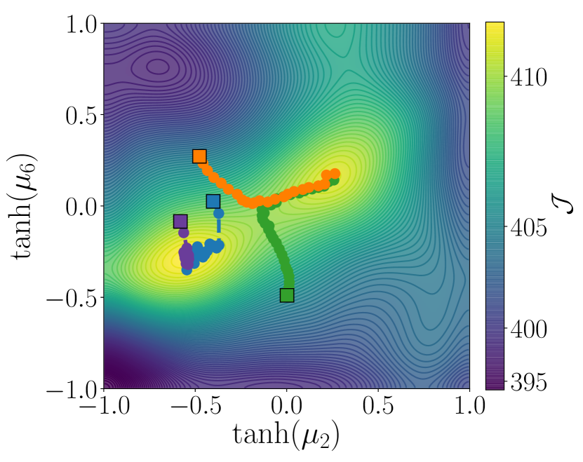
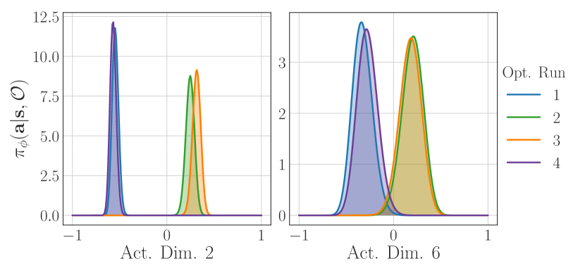
Figure 2: Estimating Multiple Policy Modes. Unlike direct amortization, which is restricted to a single estimate, iterative amortization can effectively sample from multiple high-value action modes. This is shown for a particular state in Ant-v2, showing multiple optimization runs across two action dimensions (Left). Each square denotes an initialization. The optimizer finds both modes, with the densities plotted on the Right. This capability provides increased flexibility in action exploration.

3.1 Formulation

Iterative amortization [55] utilizes errors or gradients to update the approximate posterior distribution parameters. While various forms exist, we consider gradient-encoding models [6] due to their generality. Compared with direct amortization (Eq. 10), we use iterative amortized optimizers of the general form

$$\bm{\lambda}\leftarrow f_{\phi}(\mathbf{s},\bm{\lambda},\nabla_{\bm{\lambda}}\mathcal{J}),$$ (iterative amortization) (11)

also shown in Figure 1 (Right), where $f_{\phi}$ is a deep network and $\bm{\lambda}$ are the action distribution parameters. For example, if $\pi=\mathcal{N}(\mathbf{a};\bm{\mu},\operatorname{diag}(\bm{\sigma}^{2}))$, then $\bm{\lambda}\equiv\left[\bm{\mu},\bm{\sigma}\right]$. Technically, $\mathbf{s}$ is redundant, as the state dependence is already captured in $\mathcal{J}$, but this can empirically improve performance [55]. In practice, the update is carried out using a “highway” gating operation [38, 72]. Denoting $\bm{\omega}_{\phi}\in[0,1]$ as the gate and $\bm{\delta}_{\phi}$ as the update, both of which are output by $f_{\phi}$, the gating operation is expressed as

$$\bm{\lambda}\leftarrow\bm{\omega}_{\phi}\odot\bm{\lambda}+(\mathbf{1}-\bm{\omega}_{\phi})\odot\bm{\delta}_{\phi},$$ (12)

where $\odot$ denotes element-wise multiplication. This update is typically run for a fixed number of steps, and, as with a direct policy, the iterative optimizer is trained using stochastic gradient estimates of $\nabla_{\phi}\mathcal{J}$, obtained through the path-wise derivative estimator [44, 64, 35]. Because the gradients $\nabla_{\bm{\lambda}}\mathcal{J}$ must be estimated online, i.e., during policy optimization, this scheme requires some way of estimating $\mathcal{J}$ online through a parameterized $Q$-value network [58] or a differentiable model [35].

3.2 Benefits of Iterative Amortization

Reduced Amortization Gap.

Iterative amortized optimizers are more flexible than their direct counterparts, incorporating feedback from the objective during policy optimization (Algorithm 2), rather than only after optimization (Algorithm 1). Increased flexibility improves the accuracy of optimization, thereby tightening the variational bound [55, 54]. We see this flexibility in Figure 1 (Left), where an iterative amortized policy network iteratively refines the policy estimate ($\bullet$), quickly arriving near the optimal estimate.

Multiple Estimates.

Iterative amortization, by using stochastic gradients and random initialization, can traverse the optimization landscape. As with any iterative optimization scheme, this allows iterative amortization to obtain multiple valid estimates, referred to as “multi-stability” in the generative modeling literature [27]. We illustrate this capability across two action dimensions in Figure 2 for a state in the Ant-v2 MuJoCo environment. Over multiple policy optimization runs, iterative amortization finds multiple modes, sampling from two high-value regions of the action space. This provides increased flexibility in action exploration, despite only using a uni-modal policy distribution.

Generalization Across Objectives.

Iterative amortization uses the gradients of the objective during optimization, i.e., feedback, allowing it to potentially generalize to new or updated objectives. We see this in Figure 1 (Left), where iterative amortization, despite being trained with a different value estimator, is capable of generalizing to this new objective. We demonstrate this capability further in Section 4. This opens the possibility of accurately and efficiently performing policy optimization in new settings, e.g., a rapidly changing model or new tasks.

3.3 Consideration: Mitigating Value Overestimation

Why are more powerful policy optimizers typically not used in practice? Part of the issue stems from value overestimation. Model-free approaches generally estimate $Q_{\pi}$ using function approximation and temporal difference learning. However, this has the pitfall of value overestimation, i.e., positive bias in the estimate, $\widehat{Q}_{\pi}$ [75]. This issue is tied to uncertainty in the value estimate, though it is distinct from optimism under uncertainty. If the policy can exploit regions of high uncertainty, the resulting target values will introduce positive bias into the estimate. More flexible policy optimizers exacerbate the problem, exploiting this uncertainty to a greater degree. Further, a rapidly changing policy increases the difficulty of value estimation [63].

Various techniques have been proposed for mitigating value overestimation in deep RL. The most prominent technique, double deep $Q$-network [81] maintains two $Q$-value estimates [80], attempting to decouple policy optimization from value estimation. Fujimoto et al. [25] apply and improve upon this technique for actor-critic settings, estimating the target $Q$-value as the minimum of two $Q$-networks, $Q_{\psi_{1}}$ and $Q_{\psi_{2}}$:

$$\widehat{Q}_{\pi}(\mathbf{s},\mathbf{a})=\min_{i=1,2}Q_{\psi_{i}^{\prime}}(\mathbf{s},\mathbf{a}),$$

where $\psi_{i}^{\prime}$ denotes the target network parameters. As noted by Fujimoto et al. [25], this not only counteracts value overestimation, but also penalizes high-variance value estimates, because the minimum decreases with the variance of the estimate. Ciosek et al. [15] noted that, for a bootstrapped ensemble of two $Q$-networks, the minimum operation can be interpreted as estimating

$$\widehat{Q}_{\pi}(\mathbf{s},\mathbf{a})=\mu_{Q}(\mathbf{s},\mathbf{a})-\beta\sigma_{Q}(\mathbf{s},\mathbf{a}),$$ (13)

with mean $\mu_{Q}(\mathbf{s},\mathbf{a})\equiv\frac{1}{2}\sum_{i=1,2}Q_{\psi_{i}^{\prime}}(\mathbf{s},\mathbf{a})$, standard deviation $\sigma_{Q}(\mathbf{s},\mathbf{a})\equiv(\frac{1}{2}\sum_{i=1,2}(Q_{\psi_{i}^{\prime}}(\mathbf{s},\mathbf{a})-\mu_{Q}(\mathbf{s},\mathbf{a}))^{2})^{1/2}$, and $\beta=1$. Thus, to further penalize high-variance value estimates, preventing value overestimation, we can increase $\beta$. For large $\beta$, however, value estimates become overly pessimistic, negatively impacting training. Thus, $\beta$ reduces target value variance at the cost of increased bias.

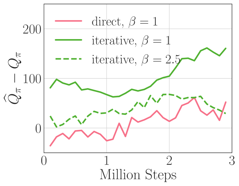
(a)

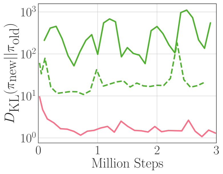
(b)

Figure 3: Mitigating Value Overestimation. With $\beta=1$, iterative amortization results in (a) higher value overestimation and (b) a more rapidly changing policy as compared with direct amortization. Increasing $\beta$ helps to mitigate these issues.

Due to the flexibility of iterative amortization, the default $\beta=1$ results in increased value bias and a more rapidly changing policy as compared with direct amortization (Figure 3). Further penalizing high-variance target values ($\beta=2.5$) reduces value overestimation and improves stability. For details, see Appendix A.2. Recent techniques for mitigating overestimation have been proposed, such as adjusting $\alpha$ [22]. In offline RL, this issue has been tackled through the action prior [24, 48, 84] or by altering $Q$-network training [2, 49]. While such techniques could be used here, increasing $\beta$ provides a simple solution with no additional computational overhead. This is a meaningful insight toward applying more powerful policy optimizers.

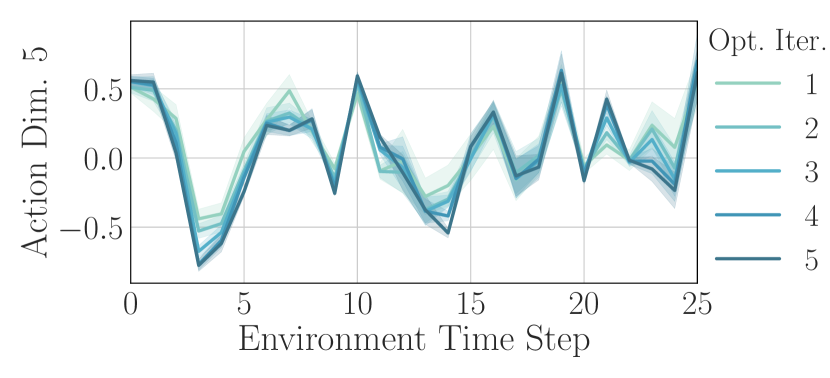
(a) Policy

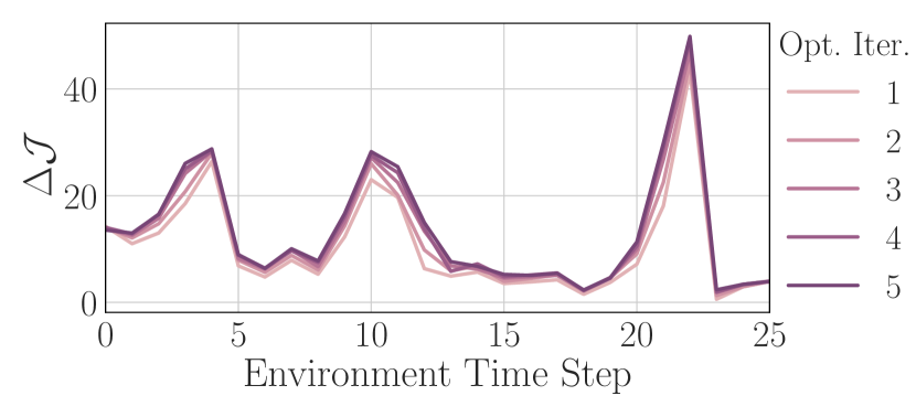
(b) Improvement

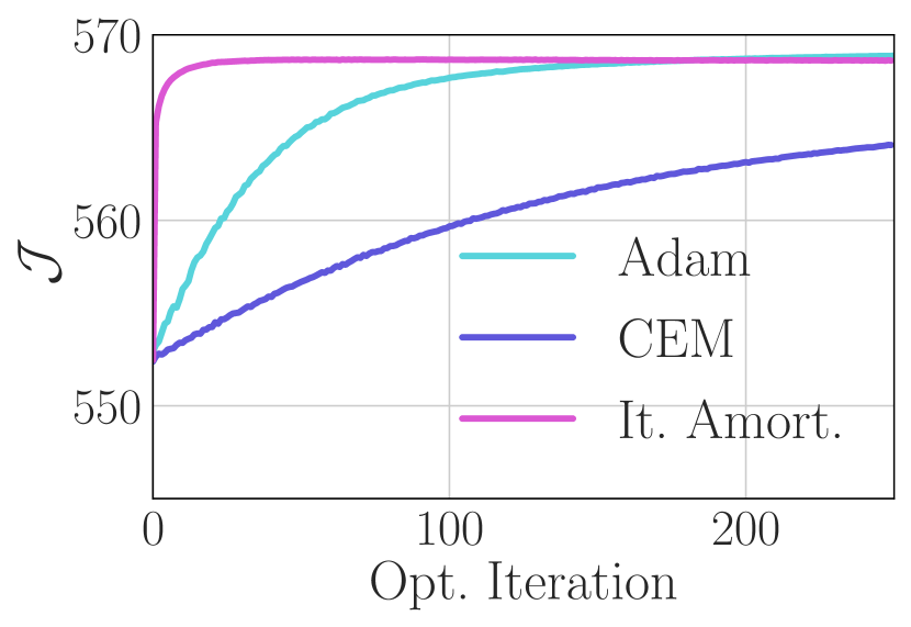
(c) Comparison

Figure 4: Policy Optimization. Visualization over time steps of (a) one dimension of the policy distribution and (b) the improvement in the objective, $\Delta\mathcal{J}$, across policy optimization iterations. (c) Comparison of iterative amortization with Adam [45] (gradient-based) and CEM [66] (gradient-free). Iterative amortization is an order of magnitude more efficient.

4 Experiments

4.1 Setup

To focus on policy optimization, we implement iterative amortized policy optimization using the soft actor-critic (SAC) setup described by Haarnoja et al. [32]. This uses two $Q$-networks, uniform action prior, $p_{\theta}(\mathbf{a}|\mathbf{s})=\mathcal{U}(-1,1)$, and a tuning scheme for the temperature, $\alpha$. In our experiments, “direct” refers to direct amortization employed in SAC, i.e., a direct policy network, and “iterative” refers to iterative amortization. Both approaches use the same network architecture, adjusting only the number of inputs and outputs to accommodate gradients, current policy estimates, and gated updates (Sec. 3.1). Unless otherwise stated, we use $5$ iterations per time step for iterative amortization, following [55]. For details, refer to Appendix A and Haarnoja et al. [31, 32].

4.2 Analysis

4.2.1 Visualizing Policy Optimization

We provide 2D visualizations of iterative amortized policy optimization in Figures 1 & 2, with additional 2D plots in Appendix B.5. In Figure 4, we visualize iterative refinement using a single action dimension from Ant-v2 across time steps. The refinements in Figure 4(a) give rise to the objective improvements in Figure 4(b). We compare with Adam [45] (gradient-based) and CEM [66] (gradient-free) in Figure 4(c), where iterative amortization is an order of magnitude more efficient. This trend is consistent across environments, as shown in Appendix B.4.

4.2.2 Performance Comparison

We evaluate iterative amortized policy optimization on the suite of MuJoCo [78] continuous control tasks from OpenAI gym [12]. In Figure 5, we compare the cumulative reward of direct and iterative amortized policy optimization across environments. Each curve shows the mean and $\pm$ standard deviation of $5$ random seeds. In all cases, iterative amortized policy optimization matches or outperforms the baseline direct amortized method, both in sample efficiency and final performance. Iterative amortization also yields more consistent, lower variance performance.

4.2.3 Improved Exploration: Multiple Policy Modes

As described in Section 3.2, iterative amortization is capable of obtaining multiple estimates, i.e., multiple modes of the optimization objective. To confirm that iterative amortization has captured multiple modes, at the end of training, we take an iterative agent trained on Walker2d-v2 and histogram the distances between policy means across separate runs of policy optimization per state (Fig. 7(a)). For the state with the largest distance, we plot 2D projections of the optimization objective, $\mathcal{J}$, across action dimensions in Figure 7(b), as well as the policy density across $10$ optimization runs (Fig. 7(c)). The multi-modal policy optimization surface shown in Figure 7(b) results in the multi-modal policy in Figure 7(c). Additional results on other environments are presented in Appendix B.7.

To better understand whether the performance benefits of iterative amortization are coming purely from improved exploration via multiple modes, we also compare with direct amortization with a multi-modal policy distribution. This is formed using inverse autoregressive flows [46], a type of normalizing flow (NF). Results are presented in Appendix B.2. Using a multi-modal policy reduces the performance deficiencies on Hopper-v2 and Walker2d-v2, indicating that much of the benefit of iterative amortization is due to lifting direct amortization’s restriction to a single, uni-modal policy estimate. Yet, direct + NF still struggles on HalfCheetah-v2 compared with iterative amortization, suggesting that more complex, multi-modal distributions are not the only consideration.

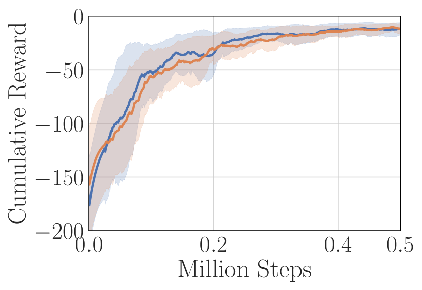
(a) Reacher-v2

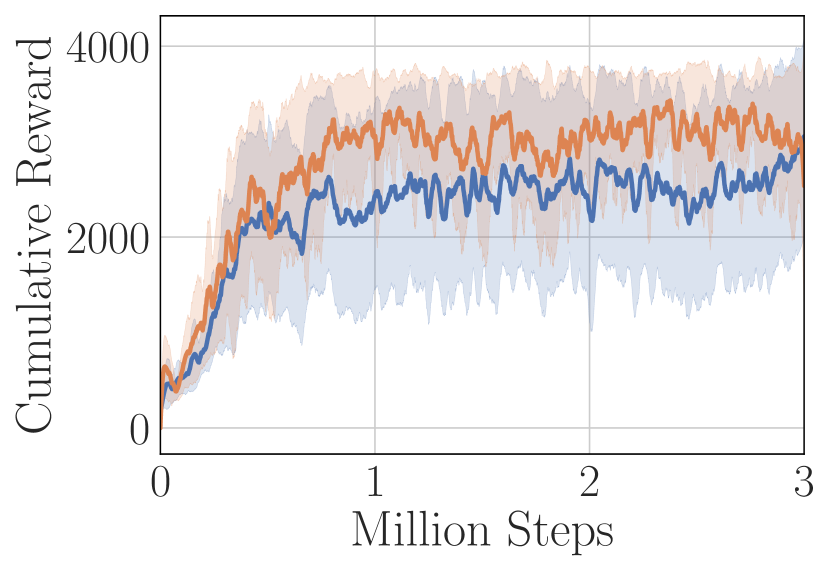
(b) Hopper-v2

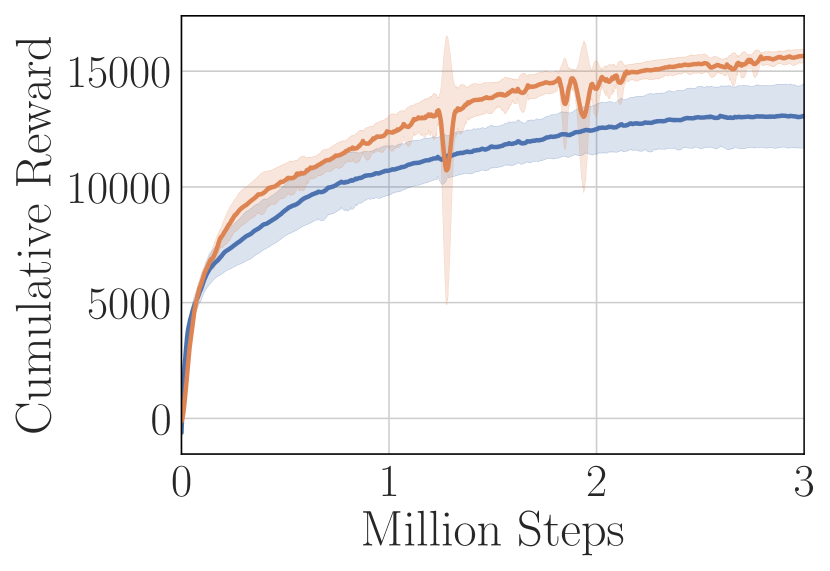
(c) HalfCheetah-v2

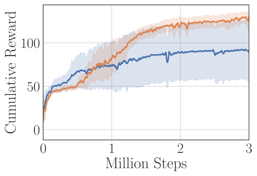
(d) Swimmer-v2

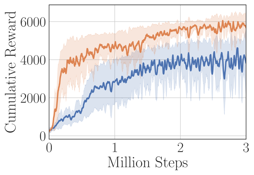
(e) Walker2d-v2

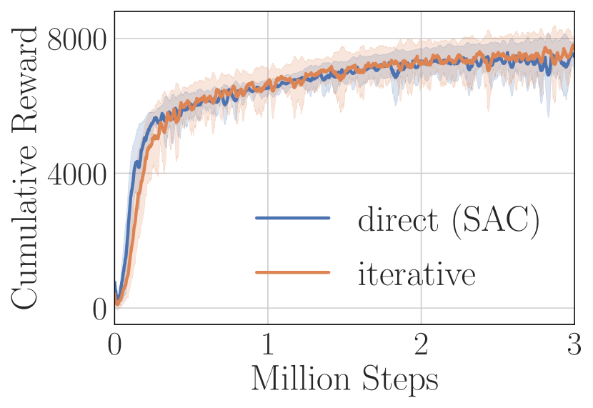
(f) Ant-v2

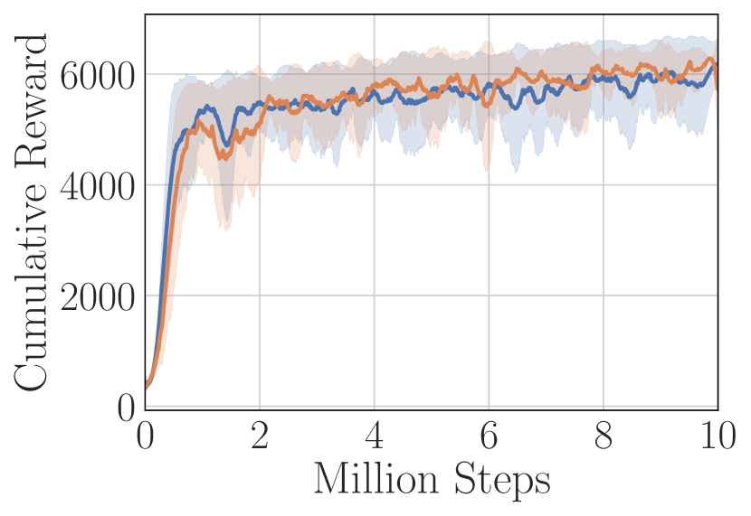
(g) Humanoid-v2

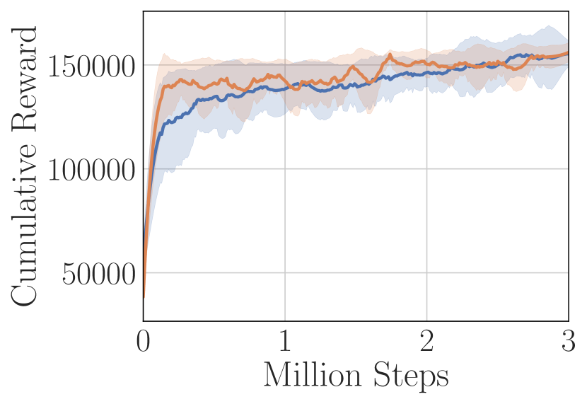
(h) HumanoidStandup-v2

Figure 5: Performance Comparison. Iterative amortized policy optimization performs comparably with or better than direct amortization across MuJoCo environments. Curves show the mean $\pm$ std. dev. of performance over $5$ random seeds.

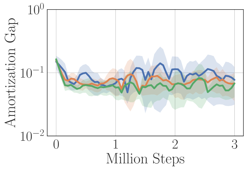
(a) Hopper-v2

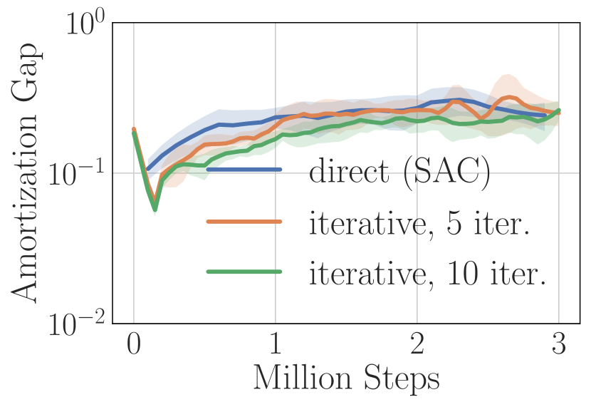
(b) HalfCheetah-v2

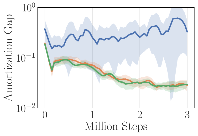
(c) Walker2d-v2

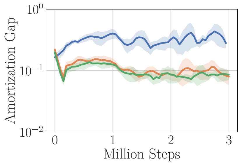
(d) Ant-v2

Figure 6: Amortization Gap. Iterative amortization achieves similar or lower amortization gaps than direct amortization. Gaps are estimated using stochastic gradient-based optimization over $100$ random states. Curves show the mean and $\pm$ std. dev. over $5$ random seeds.

4.2.4 Improved Optimization: Amortization Gap

To evaluate policy optimization accuracy, we estimate per-step amortization gaps, performing additional iterations of gradient ascent on $\mathcal{J}$ w.r.t. the policy parameters, $\bm{\lambda}\equiv\left[\bm{\mu},\bm{\sigma}\right]$ (see Appendix A.3). To analyze generalization, we also evaluate the iterative agents trained with $5$ iterations for an additional $5$ amortized iterations. Results are shown in Figure 6. We emphasize that it is challenging to directly compare amortization gaps across optimization schemes, as these involve different value functions, and therefore different objectives. Likewise, we estimate the amortization gap using the learned $Q$-networks, which may be biased (Figure 3). Nevertheless, we find that iterative amortized policy optimization achieves, on average, lower amortization gaps than direct amortization across all environments. Additional amortized iterations at evaluation yield further estimated improvement, demonstrating generalization beyond the optimization horizon used during training.

The amortization gaps are small relative to the objective, playing a negligible role in evaluation performance (see Appendix B.6). Rather, improved policy optimization is helpful for training, allowing the agent to explore states where value estimates are highest. To probe this further, we train iterative amortized policy optimization while varying the number of iterations per step in $\{1,2,5\}$, yielding optimizers with varying degrees of accuracy. Note that each optimizer is, in theory, capable of finding multiple modes. In Figure 9, we see that training with additional iterations improves performance and optimization accuracy. We stress that the exact form of this relationship depends on the $Q$-value estimator and other factors. We present additional results in Appendix B.6.

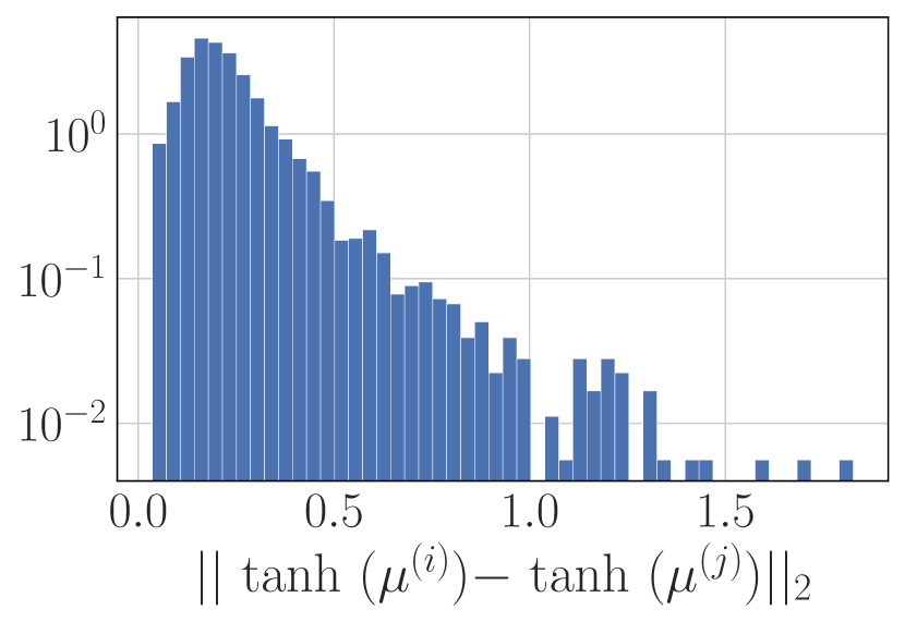
(a)

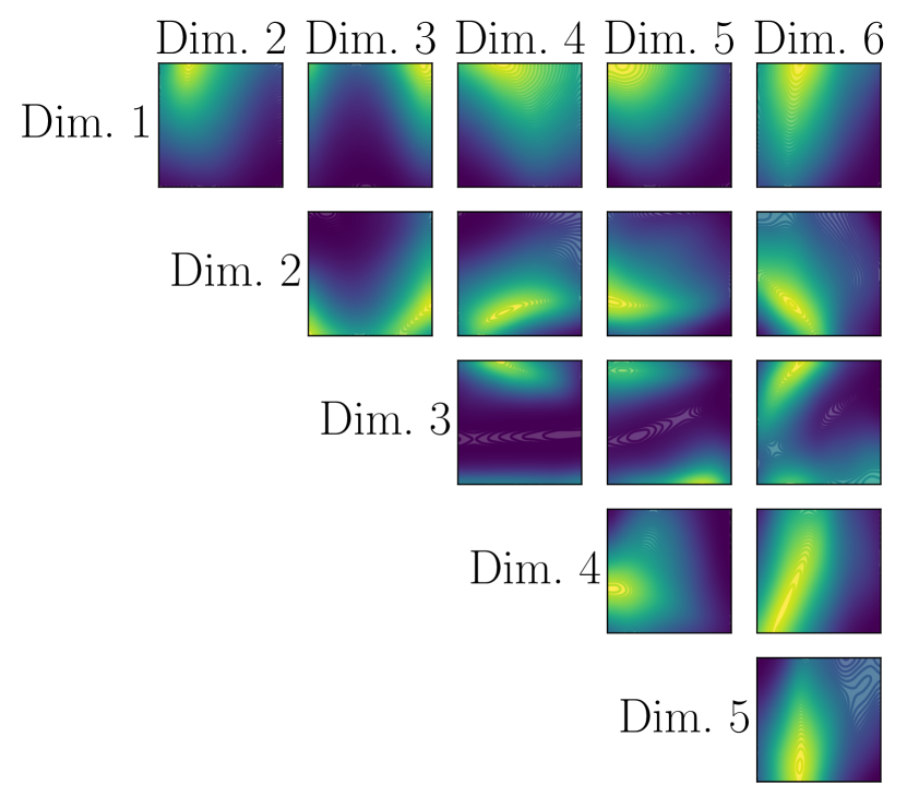
(b)

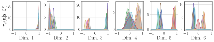
(c)

Figure 7: Multiple Policy Modes. (a) Histogram of distances between policy means ($\bm{\mu}$) across optimization runs ($i$ and $j$) over seeds and states on Walker2d-v2 at $3$ million environment steps. For the state with the largest distance, (b) shows the projected optimization surface on each pair of action dimensions, and (c) shows the policy density for $10$ optimization runs.

Figure 8: Varying Iterations During Training. Performance (Left) and estimated amortization gap (Right) for varying numbers of policy optimization iterations per step during training on HalfCheetah-v2. Increasing the iterations generally improves performance and decreases the estimated amortization gap.

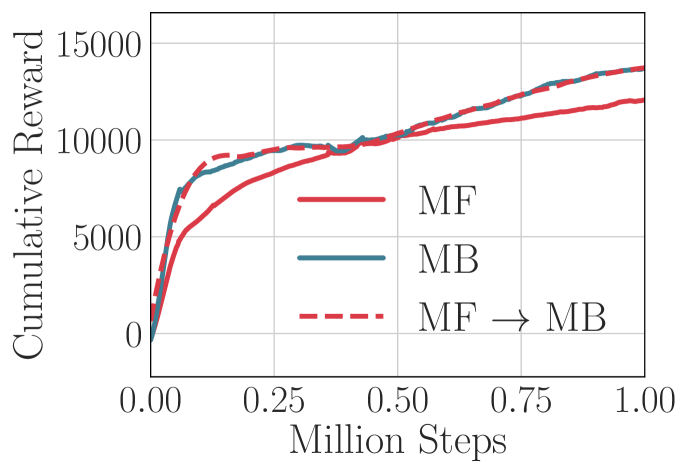
Figure 9: Zero-shot generalization of iterative amortization from model-free (MF) to model-based (MB) value estimates.

4.2.5 Generalizing to Model-Based Value Estimates

Direct amortization is a purely feedforward process and is therefore incapable of generalizing to new objectives. In contrast, because iterative amortization is formulated through gradient-based feedback, such optimizers may be capable of generalizing to new objective estimators, as shown in Figure 1. To demonstrate this capability further, we apply iterative amortization with model-based value estimators, using a learned deterministic model on HalfCheetah-v2 (see Appendix A.5). We evaluate the generalizing capabilities in Figure 9 by transferring the policy optimizer from a model-free agent to a model-based agent. Iterative amortization generalizes to these new value estimates, instantly recovering the performance of the model-based agent. This highlights the opportunity for instantly incorporating new tasks, goals, or model estimates into policy optimization.

5 Discussion

We have introduced iterative amortized policy optimization, a flexible and powerful policy optimization technique. In so doing, we have identified KL-regularized policy networks as a form of direct amortization, highlighting several limitations: 1) limited accuracy, as quantified by the amortization gap, 2) restriction to a single estimate, limiting exploration, and 3) inability to generalize to new objectives, limiting the transfer of these policy optimizers. As shown through our empirical analysis, iterative amortization provides a step toward improving each of these restrictions, with accompanying improvements in performance over direct amortization. Thus, iterative amortization can serve as a drop-in replacement and improvement over direct policy networks in deep RL.

This improvement, however, is accompanied by added challenges. As highlighted in Section 3.3, improved policy optimization can exacerbate issues in $Q$-value estimation stemming from positive bias. Note that this is not unique to iterative amortization, but applies broadly to any improved optimizer. We have provided a simple solution that involves adjusting a factor, $\beta$, to counteract this bias. Yet, we see this as an area for further investigation, perhaps drawing on insights from the offline RL community [49]. In addition to value estimation issues, iterative amortized policy optimization incurs computational costs that scale linearly with the number of iterations. This is in comparison with direct amortization, which has constant computational cost. Fortunately, unlike standard optimizers, iterative amortization adaptively tunes step sizes. Thus, relative improvements rapidly diminish with each additional iteration, enabling accurate optimization with exceedingly few iterations. In practice, even a single iteration per time step can work surprisingly well.

Although we have discussed three separate limitations of direct amortization, these factors are highly interconnected. By broadening policy optimization to an iterative procedure, we automatically obtain a potentially more accurate and general policy optimizer, with the capability of obtaining multiple modes. While our analysis suggests that improved exploration resulting from multiple modes is the primary factor affecting performance, future work could tease out these effects further and assess the relative contributions of these improvements in additional environments. We are hopeful that iterative amortized policy optimization, by providing a more powerful, exploratory, and general optimizer, will enable a range of improved RL algorithms.

Checklist

1. For all authors…

   1. Do the main claims made in the abstract and introduction accurately reflect the paper’s contributions and scope? [Yes] We demonstrate performance improvements and novel benefits of iterative amortization in Section 4. Each claim is supported by empirical evidence.

   2. Did you describe the limitations of your work? [Yes] We discuss the additional computation requirements and the necessity of mitigating value overestimation.

   3. Did you discuss any potential negative societal impacts of your work? [No] We do not see any immediate societal impacts of this work beyond the general impacts of improvements in machine learning.

   4. Have you read the ethics review guidelines and ensured that your paper conforms to them? [Yes]

2. If you are including theoretical results…

   1. Did you state the full set of assumptions of all theoretical results? [N/A]

   2. Did you include complete proofs of all theoretical results? [N/A]

3. If you ran experiments…

   1. Did you include the code, data, and instructions needed to reproduce the main experimental results (either in the supplemental material or as a URL)? [Yes] We have included code in the supplementary material with an accompanying README file.

   2. Did you specify all the training details (e.g., data splits, hyperparameters, how they were chosen)? [Yes] All details and hyperparameters are provided in the Appendix.

   3. Did you report error bars (e.g., with respect to the random seed after running experiments multiple times)? [Yes] We report error bars on each of our main quantitative results comparing performance.

   4. Did you include the total amount of compute and the type of resources used (e.g., type of GPUs, internal cluster, or cloud provider)? [Yes] We provide these details in the supplementary material.

4. If you are using existing assets (e.g., code, data, models) or curating/releasing new assets…

   1. If your work uses existing assets, did you cite the creators? [Yes] We cite the creators of the environments and software packages used in this paper.

   2. Did you mention the license of the assets? [Yes] We mention or cite the license for each asset.

   3. Did you include any new assets either in the supplemental material or as a URL? [N/A]

   4. Did you discuss whether and how consent was obtained from people whose data you’re using/curating? [N/A]

   5. Did you discuss whether the data you are using/curating contains personally identifiable information or offensive content? [N/A]

5. If you used crowdsourcing or conducted research with human subjects…

   1. Did you include the full text of instructions given to participants and screenshots, if applicable? [N/A]

   2. Did you describe any potential participant risks, with links to Institutional Review Board (IRB) approvals, if applicable? [N/A]

   3. Did you include the estimated hourly wage paid to participants and the total amount spent on participant compensation? [N/A]

Appendix A Experiment Details

Accompanying code is available at github.com/joelouismarino/variational_rl. Experiments were implemented in PyTorch [61], analyzed with NumPy [34], and visualized with Matplotlib [39] and seaborn [82]. Logging and experiment management was handled through Comet [18]. Experiments were performed on NVIDIA 1080Ti GPUs with Intel i7 8-core processors (@$4.20$GHz) on local machines, with each experiment requiring on the order of $2$ days to $1$ week to complete. We obtained the MuJoCo [78] software library through an Academic Lab license.

A.1 2D Plots

In Figures 1 and 2, we plot the estimated variational objective, $\mathcal{J}$, as a function of two dimensions of the policy mean, $\bm{\mu}$. To create these plots, we first perform policy optimization (direct amortization in Figure 1 and iterative amortization in Figure 2), estimating the policy mean and variance. This is performed using on-policy trajectories from evaluation episodes (for a direct agent in Figure 1 and an iterative agent in Figure 2). While holding all other dimensions of the policy constant, we then estimate the variational objective while varying two dimensions of the mean ($1$ & $3$ in Figure 1 and $2$ & $6$ in Figure 2). Iterative amortization is additionally performed while preventing any updates to the constant dimensions. Even in this restricted setting, iterative amortization is capable of optimizing the policy. Additional 2D plots comparing direct vs. iterative amortization on other environments are shown in Figure 19, where we see similar trends.

A.2 Value Bias Estimation

We estimate the bias in the $Q$-value estimator using a similar procedure as [25], comparing the estimate of the $Q$-networks ($\widehat{Q}_{\pi}$) with a Monte Carlo estimate of the future objective in the actual environment, $Q_{\pi}$, using a set of state-action pairs. To enable comparison across setups, we collect $100$ state-action pairs using a uniform random policy, then evaluate the estimator’s bias, $\mathbb{E}_{\mathbf{s},\mathbf{a}}\left[\widehat{Q}_{\pi}-Q_{\pi}\right]$, throughout training. To obtain the Monte Carlo estimate of $Q_{\pi}$, we use $100$ action samples, which are propagated through all future time steps. The result is discounted using the same discounting factor as used during training, $\gamma=0.99$, as well as the same Lagrange multiplier, $\alpha$. Figure 3 shows the mean and $\pm$ standard deviation across the $100$ state-action pairs.

A.3 Amortization Gap Estimation

Calculating the amortization gap in the RL setting is challenging, as properly evaluating the variational objective, $\mathcal{J}$, involves unrolling the environment. During training, the objective is estimated using a set of $Q$-networks and/or a learned model. However, finding the optimal policy distribution, $\widehat{\pi}$, under these learned value estimates may not accurately reflect the amortization gap, as the value estimator likely contains positive bias (Figure 3). Because the value estimator is typically locally accurate near the current policy, we estimate the amortization gap by performing gradient ascent on $\mathcal{J}$ w.r.t. the policy distribution parameters, $\bm{\lambda}$, initializing from the amortized estimate (from $\pi_{\phi}$). This is a form semi-amortized variational inference [37, 47, 43]. We use the Adam optimizer [45] with a learning rate of $5\times 10^{-3}$ for $100$ gradient steps, which we found consistently converged. This results in the estimated optimized $\widehat{\pi}$. We estimate the gap using $100$ on-policy states, calculating $\mathcal{J}(\theta,\widehat{\pi})-\mathcal{J}(\theta,\pi)$, i.e. the improvement in the objective after gradient-based optimization. Figure 6 shows the resulting mean and $\pm$ standard deviation. We also run iterative amortized policy optimization for an additional $5$ iterations during this evaluation, empirically yielding an additional decrease in the estimated amortization gap.

A.4 Hyperparameters

Our setup follows that of soft actor-critic (SAC) [31, 32], using a uniform action prior, i.e. entropy regularization, and two $Q$-networks [25]. Off-policy training is performed using a replay buffer [53, 58]. Training hyperparameters are given in Table 7.

Temperature

Following [32], we adjust the temperature, $\alpha$, to maintain a specified entropy constraint, $\epsilon_{\alpha}=|\mathcal{A}|$, where $|\mathcal{A}|$ is the size of the action space, i.e. the dimensionality.

Table 1: Policy Inputs & Outputs.

	Inputs	Outputs
Direct	$\mathbf{s}$	$\bm{\lambda}$
Iterative	$\mathbf{s}$, $\bm{\lambda}$, $\nabla_{\bm{\lambda}}\mathcal{J}$	$\bm{\delta}$, $\bm{\omega}$

Table 2: Policy Networks.

Hyperparameter	Value
Number of Layers	2
Number of Units / Layer	256
Non-linearity	ReLU

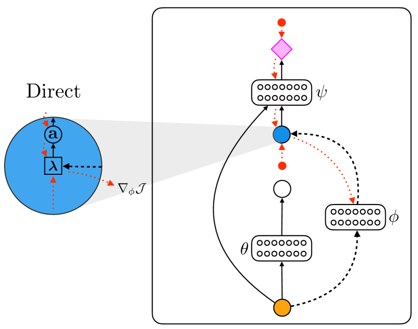
(a) Direct Amortization

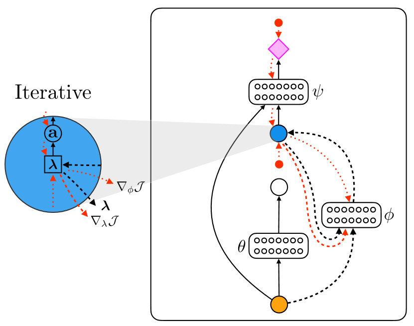
(b) Iterative Amortization

Figure 10: Amortized Optimizers. Diagrams of (a) direct and (b) iterative amortized policy optimization. As in Figure 1, larger circles represent probability distributions, and smaller red circles represent terms in the objective. Red dotted arrows represent gradients. In addition to the state, $\mathbf{s}_{t}$, iterative amortization uses the current policy distribution estimate, $\bm{\lambda}$, and the policy optimization gradient, $\nabla_{\bm{\lambda}}\mathcal{J}$, to iteratively optimize $\mathcal{J}$. Like direct amortization, the optimizer network parameters, $\phi$, are updated using $\nabla_{\phi}\mathcal{J}$. This generally requires some form of stochastic gradient estimation to differentiate through $\mathbf{a}_{t}\sim\pi(\mathbf{a}_{t}|\mathbf{s}_{t},\mathcal{O};\bm{\lambda})$.

Policy

We use the same network architecture (number of layers, units/layer, non-linearity) for both direct and iterative amortized policy optimizers (Table 2). Each policy network results in Gaussian distribution parameters, and we apply a tanh transform to ensure $\mathbf{a}\in[-1,1]$ [31]. In the case of a Gaussian, the distribution parameters are $\bm{\lambda}=\left[\bm{\mu},\bm{\sigma}\right]$. The inputs and outputs of each optimizer form are given in Table 2. Again, $\bm{\delta}$ and $\bm{\omega}$ are respectively the update and gate of the iterative amortized optimizer (Eq. 12 in the main text), each of which are defined for both $\bm{\mu}$ and $\bm{\sigma}$. Following [55], we apply layer normalization [9] individually to each of the inputs to iterative amortized optimizers. We initialize iterative amortization with $\bm{\mu}=\mathbf{0}$ and $\bm{\sigma}=\mathbf{1}$, however, these could be initialized from a learned action prior [54].

Table 3: $Q$-value Network Architecture A.

Hyperparameter	Value
Number of Layers	2
Number of Units / Layer	256
Non-linearity	ReLU
Layer Normalization	False
Connectivity	Sequential

Table 4: $Q$-value Network Architecture B.

Hyperparameter	Value
Number of Layers	3
Number of Units / Layer	512
Non-linearity	ELU
Layer Normalization	True
Connectivity	Highway

$Q$-value

We investigated two $Q$-value network architectures. Architecture A (Table 4) is the same as that from [31]. Architecture B (Table 4) is a wider, deeper network with highway connectivity [72], layer normalization [9], and ELU nonlinearities [17]. We initially compared each $Q$-value network architecture using each policy optimizer on each environment, as shown in Figure 11. The results in Figure 5 were obtained using the better performing architecture in each case, given in Tables 5 & 6. As in [25], we use an ensemble of $2$ separate $Q$-networks in each experiment.

Table 5: $Q$-value Network Architecture by Environment.

	InvertedPendulum-v2	InvertedDoublePendulum-v2	Hopper-v2	HalfCheetah-v2	Walker2d-v2	Ant-v2
Direct	A	A	A	B	A	B
Iterative	A	A	A	A	B	B

Table 6: $Q$-value Network Architecture by Environment (Continued).

	Reacher-v2	Swimmer-v2	Humanoid-v2	HumanoidStandup-v2
Direct	A	A	B	B
Iterative	A	A	B	B

Value Pessimism ($\beta$)

As discussed in Section 3.2.2, the increased flexibility of iterative amortization allows it to potentially exploit inaccurate value estimates. We increased the pessimism hyperparameter, $\beta$, to further penalize variance in the value estimate. Experiments with direct amortization use the default $\beta=1$ in all environments, as we did not find that increasing $\beta$ helped in this setup. For iterative amortization, we use $\beta=1.5$ on Hopper-v2 and $\beta=2.5$ on all other environments. This is only applied during training; while collecting data in the environment, we use $\beta=1$ to not overly penalize exploration.

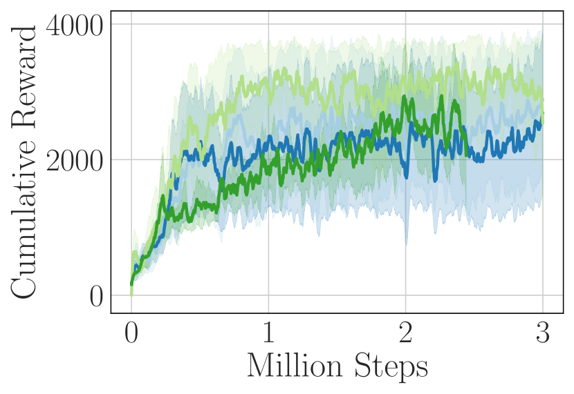
(a) Hopper-v2

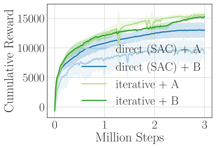
(b) HalfCheetah-v2

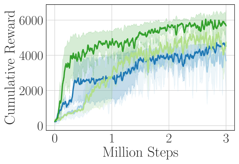
(c) Walker2d-v2

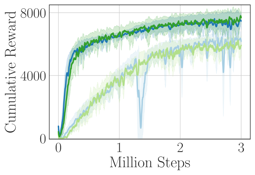
(d) Ant-v2

Figure 11: Value Architecture Comparison. Plots show performance for $\geq 3$ seeds for each value architecture (A or B) for each policy optimization technique (direct or iterative). Note: results for iterative $+$ B on Hopper-v2 were obtained with an overly pessimistic value estimate ($\beta=2.5$ rather than $\beta=1.5$) and are consequently worse.

Table 7: Training Hyperparameters.

Hyperparameter	Value
Discount Factor $(\gamma)$	$0.99$
$Q$-network Update Rate $(\tau)$	$5\cdot 10^{-3}$
Network Optimizer	Adam
Learning Rate	$3\cdot 10^{-4}$
Batch Size	$256$
Initial Random Steps	$5\cdot 10^{3}$
Replay Buffer Size	$10^{6}$

A.5 Model-Based Value Estimation

For model-based experiments, we use a single, deterministic model together with the ensemble of $2$ $Q$-value networks (discussed above).

Model

We use separate networks to estimate the state transition dynamics, $p_{\textrm{env}}(\mathbf{s}_{t+1}|\mathbf{s}_{t},\mathbf{a}_{t})$, and reward function, $r(\mathbf{s}_{t},\mathbf{a}_{t})$. The network architecture is given in Table 9. Each network outputs the mean of a Gaussian distribution; the standard deviation is a separate, learnable parameter. The reward network directly outputs the mean estimate, whereas the state transition network outputs a residual estimate, $\Delta_{\mathbf{s}_{t}}$, yielding an updated mean estimate through:

$$\bm{\mu}_{\mathbf{s}_{t+1}}=\mathbf{s}_{t}+\Delta_{\mathbf{s}_{t}}.$$

Table 8: Model Network Architectures.

Hyperparameter	Value
Number of Layers	2
Number of Units / Layer	256
Non-linearity	Leaky ReLU
Layer Normalization	True

Table 9: Model-Based Hyperparameters.

Hyperparameter	Value
Rollout Horizon, $h$	2
Retrace $\lambda$	0.9
Pre-train Model Updates	$10^{3}$
Model-Based Value Targets	True

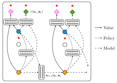
Figure 12: Model-Based Value Estimation. Diagram of model-based value estimation (shown with direct amortization). For clarity, the diagram is shown without the policy prior network, $p_{\theta}(\mathbf{a}_{t}|\mathbf{s}_{t})$. The model consists of a deterministic reward estimate, $r(\mathbf{s}_{t},\mathbf{a}_{t})$, (green diamond) and a state estimate, $\mathbf{s}_{t+1}|\mathbf{s}_{t},\mathbf{a}_{t}$, (orange diamond). The model is unrolled over a horizon, $H$, and the $Q$-value is estimated using the Retrace estimator [59], given in Eq. 14.

Model Training

The state transition and reward networks are both trained using maximum log-likelihood training, using data examples from the replay buffer. Training is performed at the same frequency as policy and $Q$-network training, using the same batch size ($256$) and network optimizer. However, we perform $10^{3}$ updates at the beginning of training, using the initial random steps, in order to start with a reasonable model estimate.

Value Estimation

To estimate $Q$-values, we combine short model rollouts with the model-free estimates from the $Q$-networks. Specifically, we unroll the model and policy, obtaining state, reward, and policy estimates at current and future time steps. We then apply the $Q$-value networks to these future state-action estimates. Future rewards and value estimates are combined using the Retrace estimator [59]. Denoting the estimate from the $Q$-network as $\widehat{Q}_{\psi}(\mathbf{s},\mathbf{a})$ and the reward estimate as $\widehat{r}(\mathbf{s},\mathbf{a})$, we calculate the $Q$-value estimate at the current time step as

$$\widehat{Q}_{\pi}(\mathbf{s}_{t},\mathbf{a}_{t})=\widehat{Q}_{\psi}(\mathbf{s}_{t},\mathbf{a}_{t})+\mathbb{E}\left[\sum_{t^{\prime}=t}^{t+h}\gamma^{t^{\prime}-t}\lambda^{t^{\prime}-t}\delta_{t^{\prime}}\right],$$ (14)

where $\delta_{t^{\prime}}$ is the estimated temporal difference:

$$\delta_{t^{\prime}}\equiv\widehat{r}(\mathbf{s}_{t^{\prime}},\mathbf{a}_{t^{\prime}})+\gamma\widehat{V}_{\psi}(\mathbf{s}_{t^{\prime}+1})-\widehat{Q}_{\psi}(\mathbf{s}_{t^{\prime}},\mathbf{a}_{t^{\prime}}),$$ (15)

$\lambda$ is an exponential weighting factor, $h$ is the rollout horizon, and the expectation is evaluated under the model and policy. In the variational RL setting, the state-value, $V_{\pi}(\mathbf{s})$, is

$$V_{\pi}(\mathbf{s})=\mathbb{E}_{\pi}\left[Q_{\pi}(\mathbf{s},\mathbf{a})-\alpha\log\frac{\pi(\mathbf{a}|\mathbf{s},\mathcal{O})}{p_{\theta}(\mathbf{a}|\mathbf{s})}\right].$$ (16)

In Eq. 14, we approximate $V_{\pi}$ using the $Q$-network to approximate $Q_{\pi}$ in Eq. 16, yielding $\widehat{V}_{\psi}(\mathbf{s})$. Finally, to ensure consistency between the model and the $Q$-value networks, we use the model-based estimate from Eq. 14 to provide target values for the $Q$-networks, as in [40].

Future Policy Estimates

Evaluating the expectation in Eq. 14 requires estimates of $\pi$ at future time steps. This is straightforward with direct amortization, which employs a feedforward policy, however, with iterative amortization, this entails recursively applying an iterative optimization procedure. Alternatively, we could use the prior, $p_{\theta}(\mathbf{a}|\mathbf{s})$, at future time steps, but this does not apply in the max-entropy setting, where the prior is uniform. For computational efficiency, we instead learn a separate direct (amortized) policy for model-based rollouts. That is, with iterative amortization, we create a separate direct network using the same hyperparameters from Table 2. This network distills iterative amortization into a direct amortized optimizer, through the KL divergence, $D_{\textrm{KL}}(\pi_{\textrm{it.}}||\pi_{\textrm{dir.}})$. Rollout policy networks are common in model-based RL [69, 62].

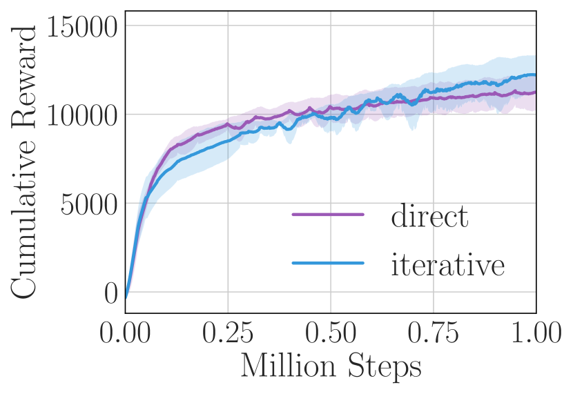
(a) Performance

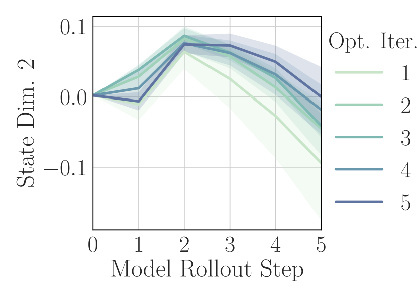
(b) Planning

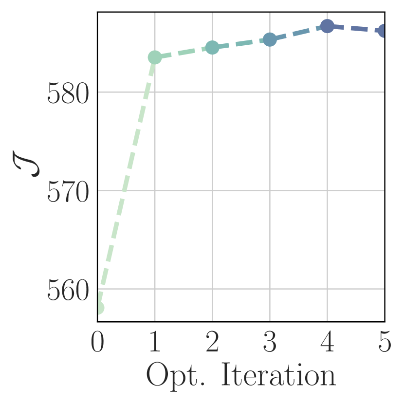
(c) Improvement

Figure 13: Model-Based Value Estimates. (a) Performance comparison of direct and iterative amortization using model-based value estimates. Curves show the mean and $\pm$ std. dev. over $4$ random seeds. (b) Planned trajectories over policy optimization iterations. (c) The corresponding estimated objective increases over iterations.

Model-Based Results

In Figure 13, we show results using iterative amortization with model-based value estimates. Iterative amortization offers a slight improvement over direct amortization in terms of performance at $1$ million steps. As in the model-free case, iterative amortization results in improvement over iterations (Fig. 13(c)), but now as a result of planning trajectories (Fig. 13(b)).

Appendix B Additional Results

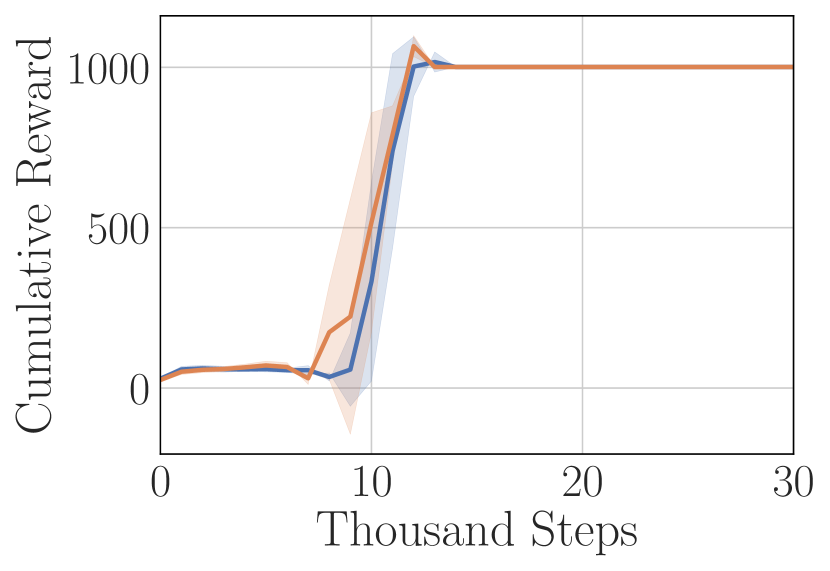
(a) InvertedPendulum-v2

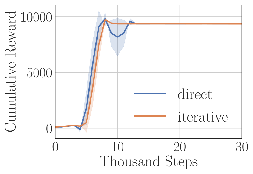
(b) InvertedDoublePendulum-v2

Figure 14: Pendulum Performance Comparison. Curves show the mean and $\pm$ std. dev. over $5$ random seeds.

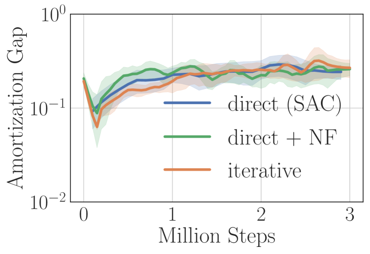
Figure 15: Amortization Gap for direct + NF on HalfCheetah-v2.

B.1 Pendulum Environments

In Figure 15, we present additional results on the remaining two MuJoCo environments from OpenAI gym: InvertedPendulum-v2 and InvertedDoublePendulum-v2. The curves show the mean and standard deviation over $5$ random seeds. Iterative amortization performs comparably with direct amortization on these simpler environments.

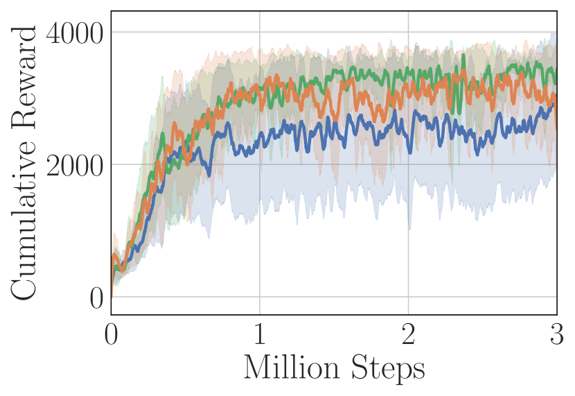
(a) Hopper-v2

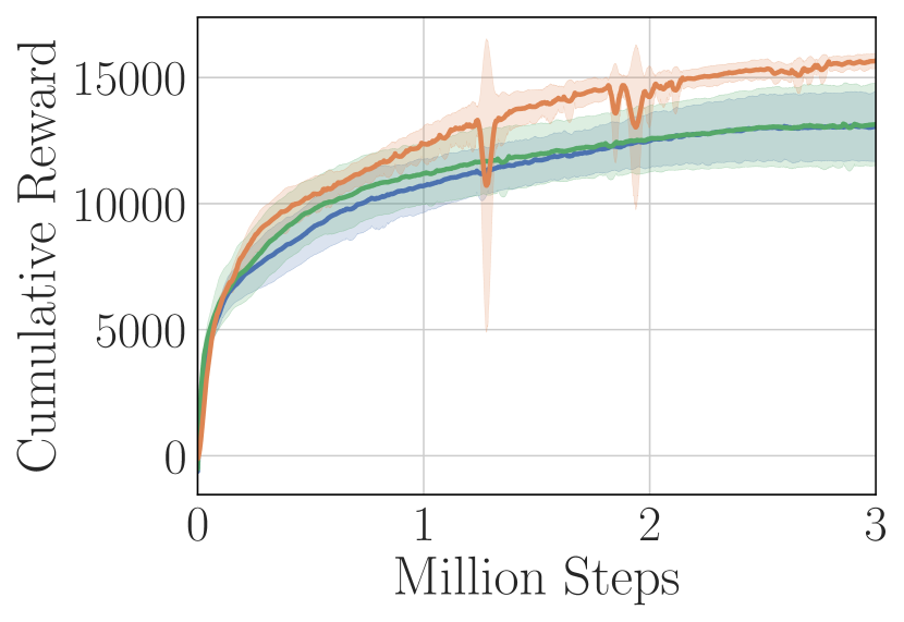
(b) HalfCheetah-v2

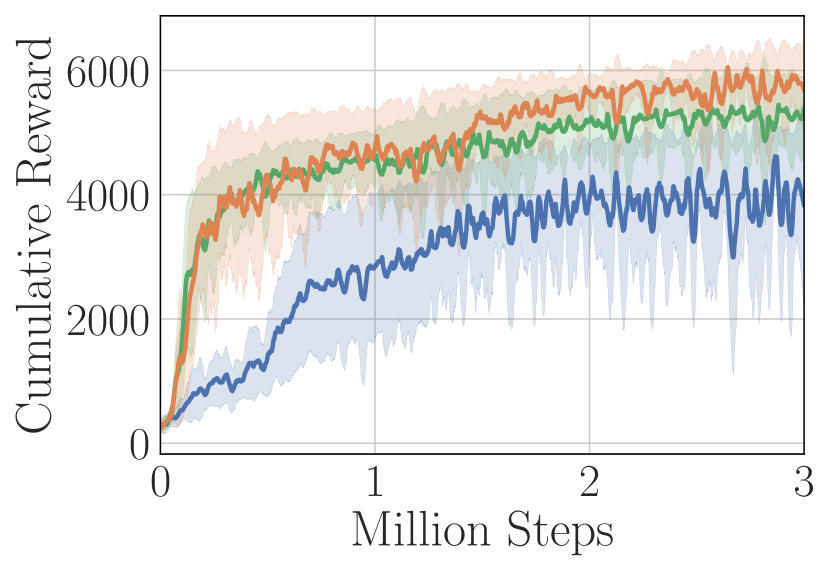
(c) Walker2d-v2

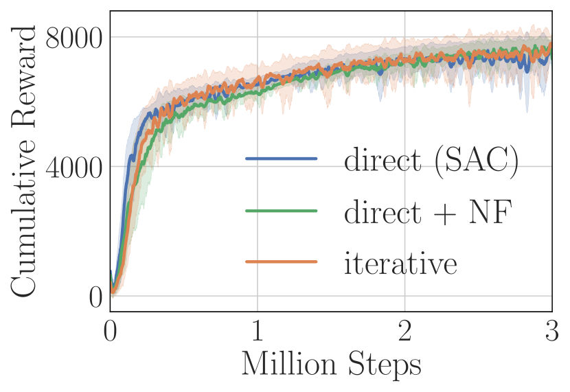
(d) Ant-v2

Figure 16: Performance Comparison with NF Policies. Curves show the mean $\pm$ std. dev. of performance over $5$ random seeds.

B.2 Comparison with Normalizing Flow-Based Policies

Iterative amortization is capable of estimating multiple policy modes, potentially yielding improved exploration. Thus, the benefits of iterative amortization may come purely from this effective improvement in the policy distribution. To test this hypothesis, we compare with direct amortization with normalizing flow-based (NF) policies, formed using two inverse autoregressive flow transforms [46]. Each transform is parameterized by a network with $2$ layers of $256$ units with ReLU activation, and we reverse the action dimension ordering between the transforms to model dependencies in both directions. In Figure 16, we plot performance on a subset of environments, where we see that direct + NF closes the performance gap on Hopper-v2 and Walker2d-v2 but is unable to close the gap on HalfCheetah-v2. In Figure 15, we see that direct + NF is also unable to close the amortization gap early on during training. Thus, improved optimization of iterative amortization, rather than purely improved exploration, does appear to play some role in the performance improvements.

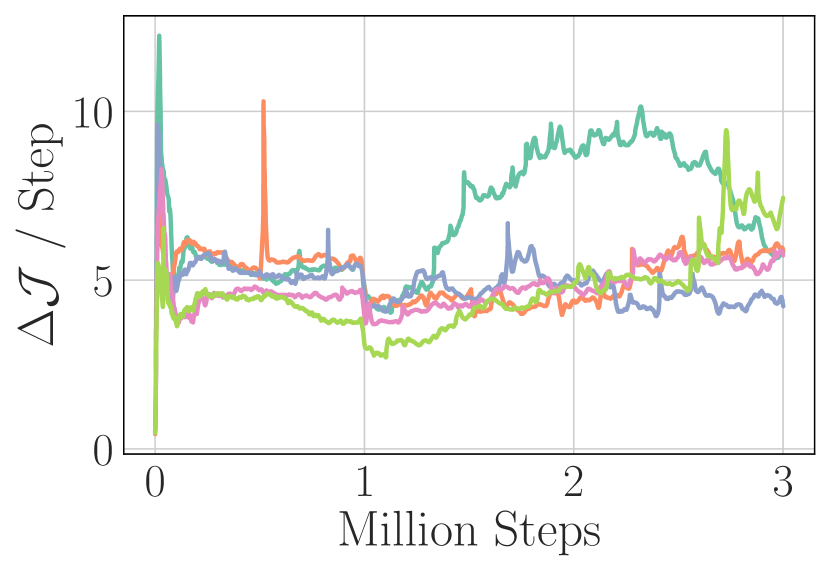
(a) Hopper-v2

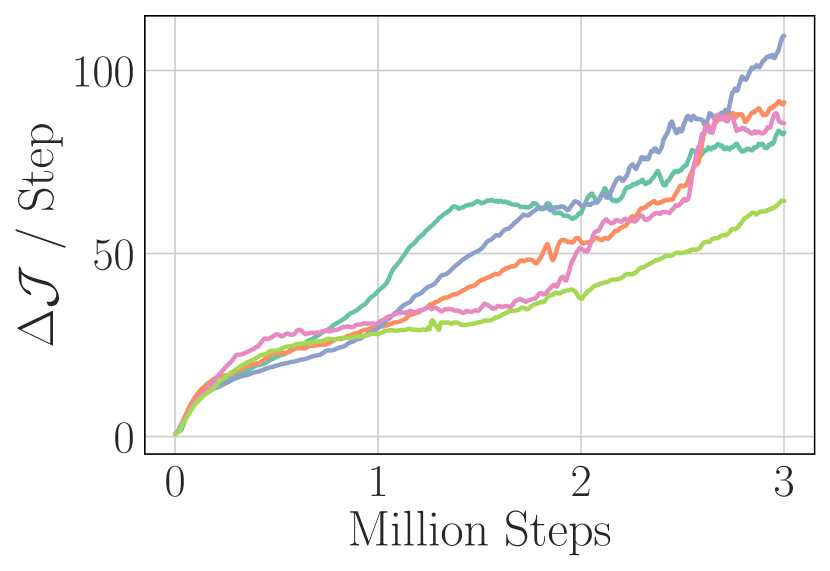
(b) HalfCheetah-v2

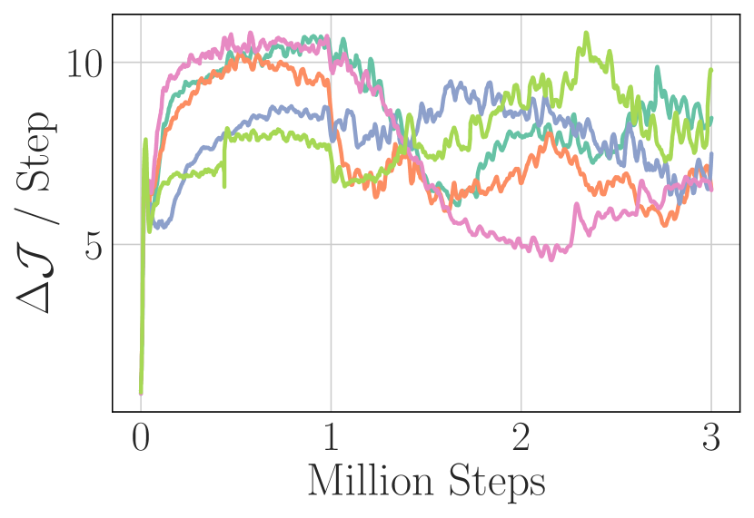
(c) Walker2d-v2

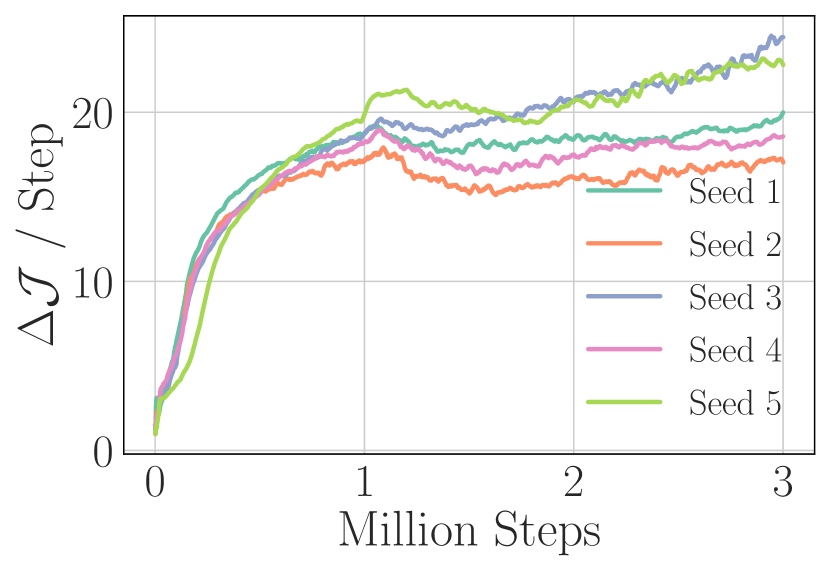
(d) Ant-v2

Figure 17: Per-Step Improvement. Each plot shows the per-step improvement in the estimated variational RL objective, $\mathcal{J}$, throughout training resulting from iterative amortized policy optimization. Each curve denotes a different random seed.

B.3 Improvement per Step

In Figure 17, we plot the average improvement in the variational objective per step throughout training, with each curve showing a different random seed. That is, each plot shows the average change in the variational objective after running $5$ iterations of iterative amortized policy optimization. With the exception of HalfCheetah-v2, the improvement remains relatively constant throughout training and consistent across seeds.

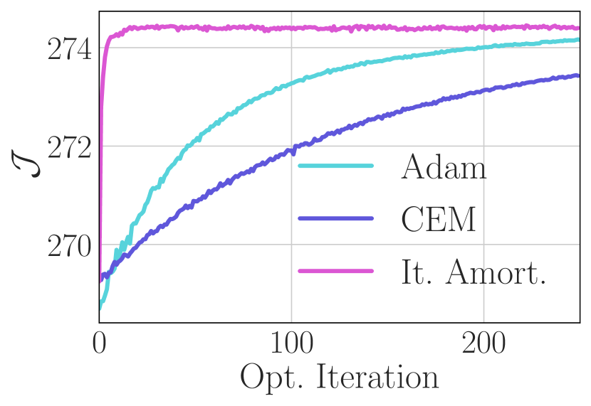
(a) Hopper-v2

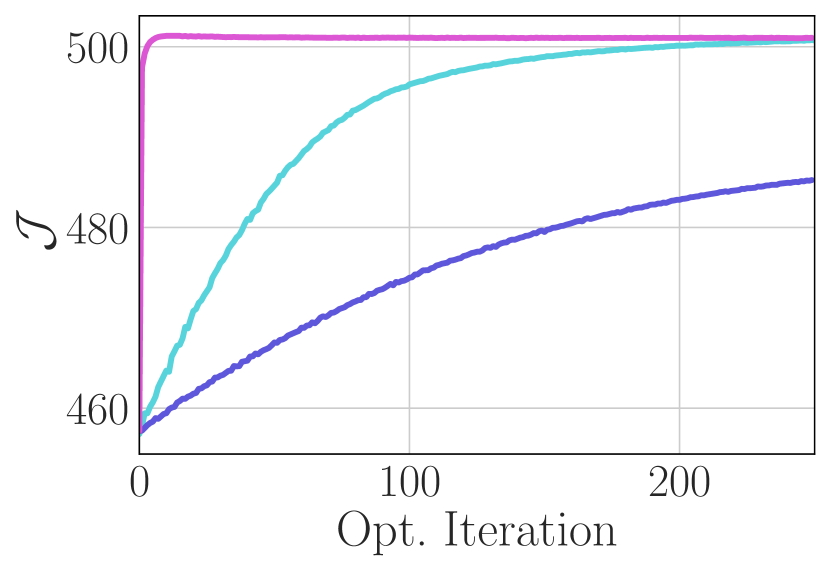
(b) HalfCheetah-v2

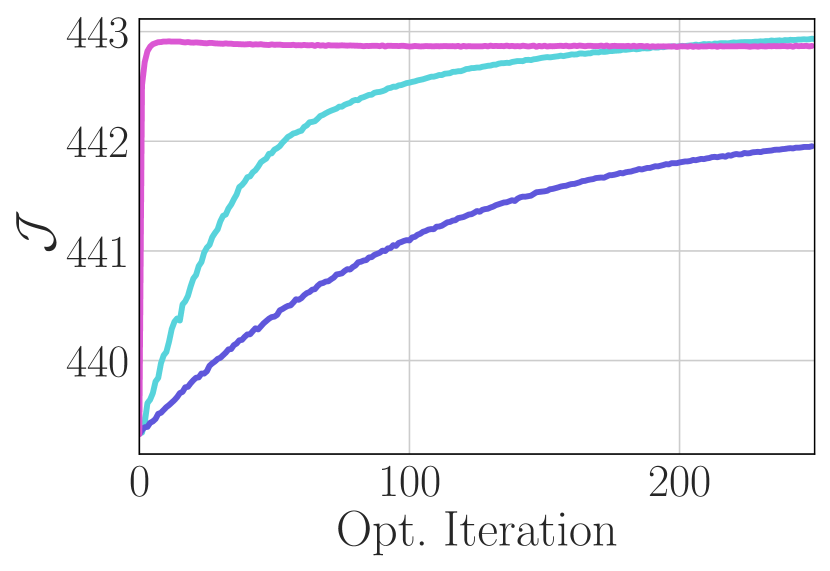
(c) Walker2d-v2

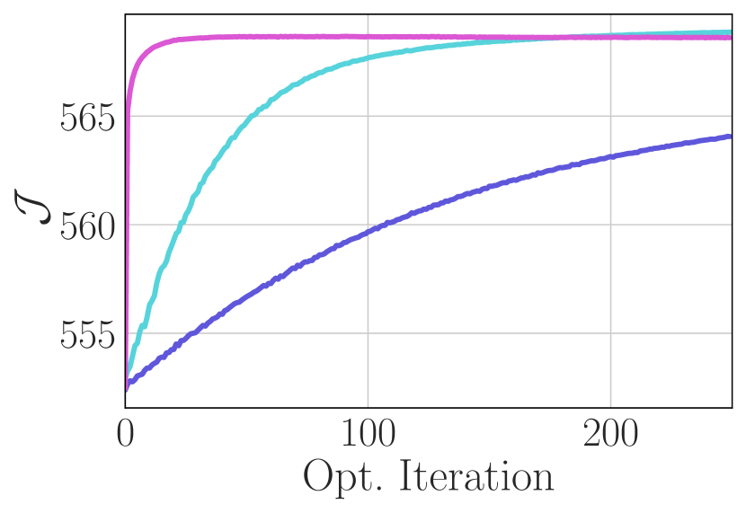
(d) Ant-v2

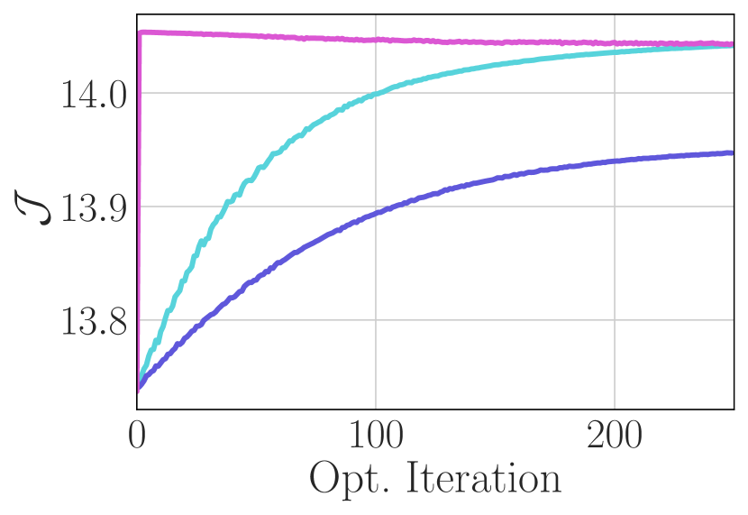
(e) Swimmer-v2

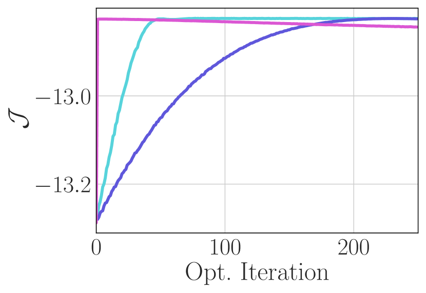
(f) Reacher-v2

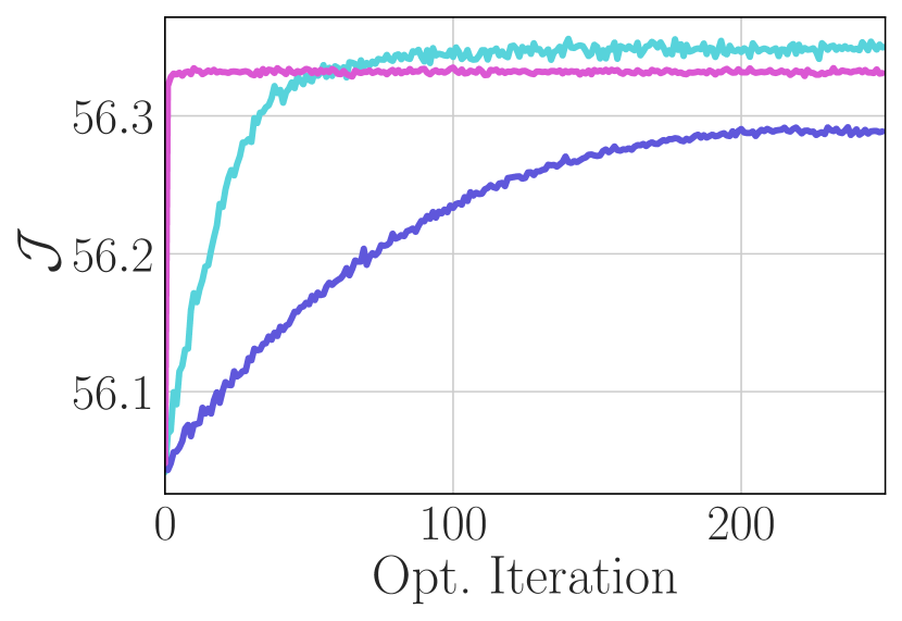
(g) InvertedPendulum-v2

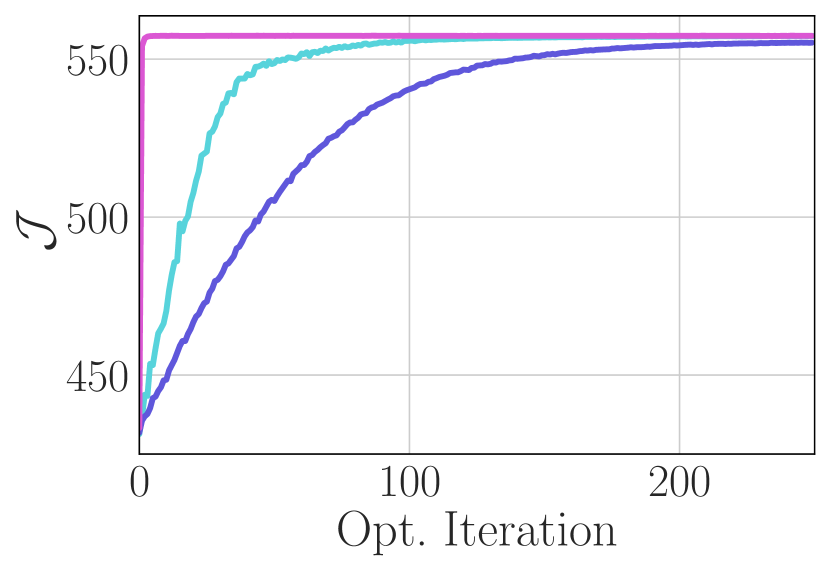
(h) InvertedDoublePendulum-v2

Figure 18: Comparison with Iterative Optimizers. Average estimated objective over policy optimization iterations, comparing with Adam [45] and CEM [66]. These iterative optimizers require over an order of magnitude more iterations to reach comparable performance with iterative amortization, making them impractical in many applications.

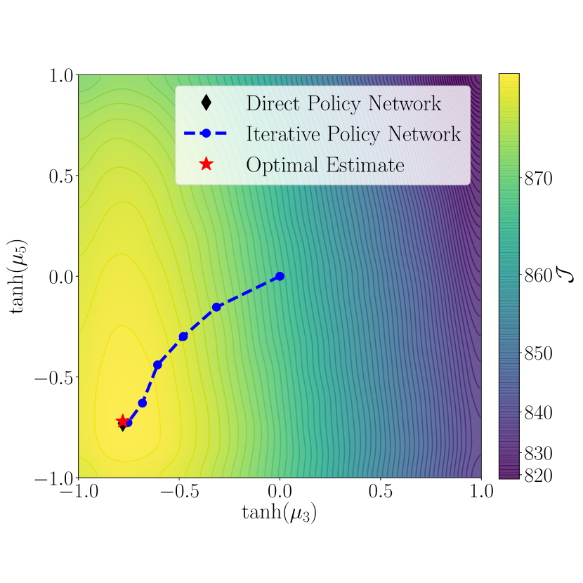
(a) HalfCheetah-v2

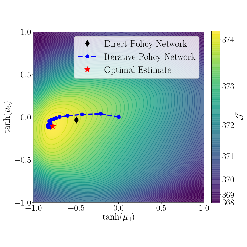
(b) Walker2d-v2

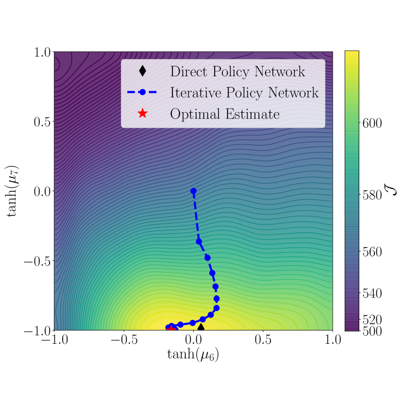
(c) Ant-v2

Figure 19: 2D Optimization Plots. Each plot shows the optimization objective over two dimensions of the policy mean, $\bm{\mu}$. This optimization surface contains the value function trained using a direct amortized policy. The black diamond, denoting the estimate of this direct policy, is generally near-optimal, but does not match the optimal estimate (red star). Iterative amortized optimizers are capable of generalizing to these surfaces in each case, reaching optimal policy estimates.

B.4 Comparison with Iterative Optimizers

Iterative amortized policy optimization obtains the accuracy benefits of iterative optimization while retaining the efficiency benefits of amortization. In Section 4, we compared the accuracy of iterative and direct amortization, seeing that iterative amortization yields reduced amortization gaps (Figure 6) and improved performance (Figure 5). In this section, we compare iterative amortization with two popular iterative optimizers: Adam [45], a gradient-based optimizer, and cross-entropy method (CEM) [66], a gradient-free optimizer.

To compare the accuracy and efficiency of the optimizers, we collect $100$ states for each seed in each environment from the model-free experiments in Section 4.2.2. For each optimizer, we optimize the variational objective, $\mathcal{J}$, starting from the same initialization. Tuning the step size, we found that $0.01$ yielded the steepest improvement without diverging for both Adam and CEM. Gradients are evaluated with $10$ action samples. For CEM, we sample $100$ actions and fit a Gaussian mean and variance to the top $10$ samples. This is comparable with QT-Opt [41], which draws $64$ samples and retains the top $6$ samples.

The results, averaged across states and random seeds, are shown in Figure 18. CEM (gradient-free) is less efficient than Adam (gradient-based), which is unsurprising, especially considering that Adam effectively approximates higher-order curvature through momentum terms. However, Adam and CEM both require over an order of magnitude more iterations to reach comparable performance with iterative amortization. While iterative amortized policy optimization does not always obtain asymptotically optimal estimates, we note that these networks were trained with only $5$ iterations, yet continue to improve and remain stable far beyond this limit. Finally, comparing wall clock time for each optimizer, iterative amortization is only roughly $1.25\times$ slower than CEM and $1.15\times$ slower than Adam, making iterative amortization still substantially more efficient.

B.5 Additional 2D Optimization Plots

In Figure 1, we provided an example of suboptimal optimization resulting from direct amortization on the Hopper-v2 environment. We also demonstrated that iterative amortization is capable of automatically generalizing to this optimization surface, outperforming the direct amortized policy. To show that this is a general phenomenon, in Figure 19, we present examples of corresponding 2D plots for each of the other environments considered in this paper. As before, we see that direct amortization is near-optimal, but, in some cases, does not match the optimal estimate. In contrast, iterative amortization is able to find the optimal estimate, again, generalizing to the unseen optimization surfaces.

B.6 Additional Optimization & the Amortization Gap

In Section 4, we compared the performance of direct and iterative amortization, as well as their estimated amortization gaps. In this section, we provide additional results analyzing the relationship between policy optimization and the performance in the actual environment. As emphasized in the main paper, this relationship is complex, as optimizing an inaccurate $Q$-value estimate does not improve task performance. Likewise, optimization improvement accrues over the course of training, facilitating collecting high-value state-action pairs in the environment.

The amortization gap quantifies the suboptimality in the objective, $\mathcal{J}$, of the policy estimate. As described in Section A.3, we estimate the optimized policy by performing additional gradient-based optimization on the policy distribution parameters (mean and variance). However, as noted, this gap is relatively small compared to the objective itself. Thus, when we deploy this optimized policy for evaluation in the actual environment, as shown for direct amortization in Figure 20, we do not observe a noticeable difference in performance.

Likewise, in Section 4.2.2, we observed that using additional amortized iterations during evaluation further decreased the amortization gap for iterative amortization. Yet, when we deploy this more fully optimized policy in the environment, as shown in Figure 21, we do not generally observe a corresponding performance improvement. In fact, on HalfCheetah-v2 and Walker2d-v2, we observe a slight decrease in performance. This further highlights the fact that additional policy optimization may exploit inaccurate $Q$-value estimates.

However, importantly, in Figures 20 and 21, the additional policy optimization is only performed for evaluation. That is, the data collected with the more fully optimized policy is not used for training and therefore cannot be used to correct the inaccurate value estimates. Thus, while more accurate policy optimization, as quantified by the amortization gap, may not substantially affect evaluation performance, it can play a role in improving training.

This aspect is explored in Figures 22 & 23, where we plot the performance and amortization gap of iterative amortization with varying numbers of iterations ($1$, $2$ and $5$) throughout training. While the trend is not exact in all cases, we generally observe that increasing iterations yields improved performance and more accurate optimization. Walker2d-v2 provides an interesting example. Even with a single iteration, we see that iterative amortization outperforms direct amortization, suggesting that multi-modality is the dominant factor for improved performance here. Yet, $1$ iteration is slightly worse compared with $2$ and $5$ iterations early in training, both in terms of performance and optimization. As the amortization gap decreases later in training, we see that the performance gap ultimately decreases. Further work could help to analyze this process in even more detail.

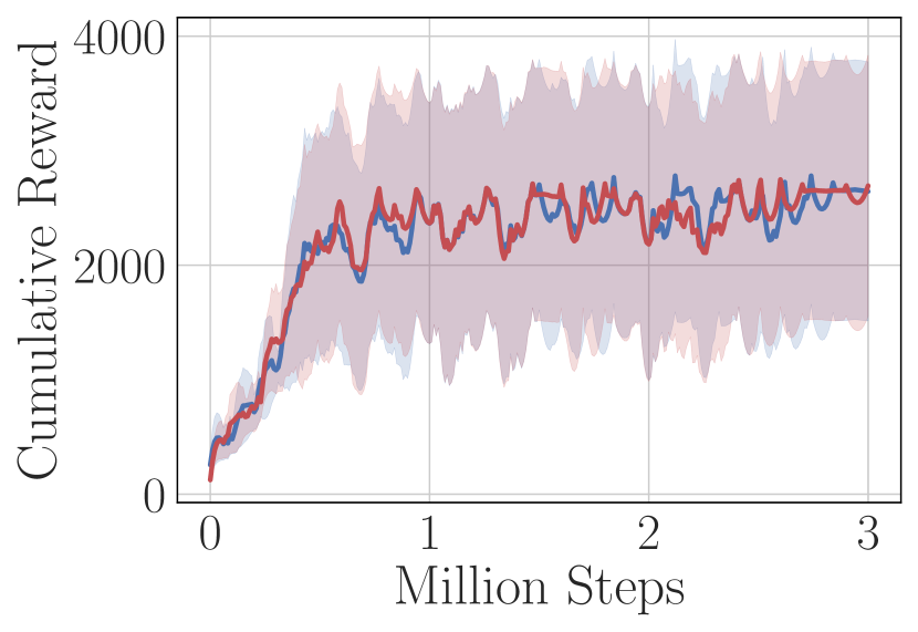
(a) Hopper-v2

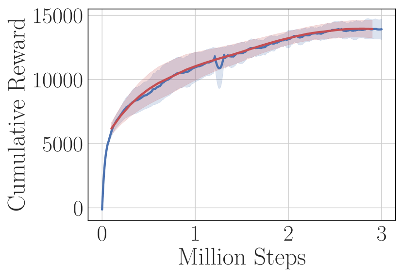
(b) HalfCheetah-v2

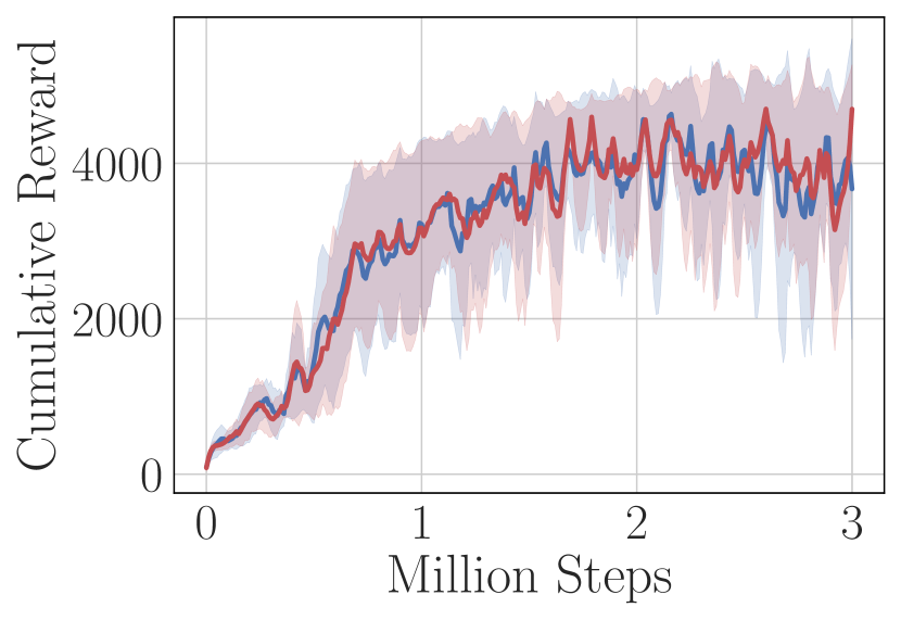
(c) Walker2d-v2

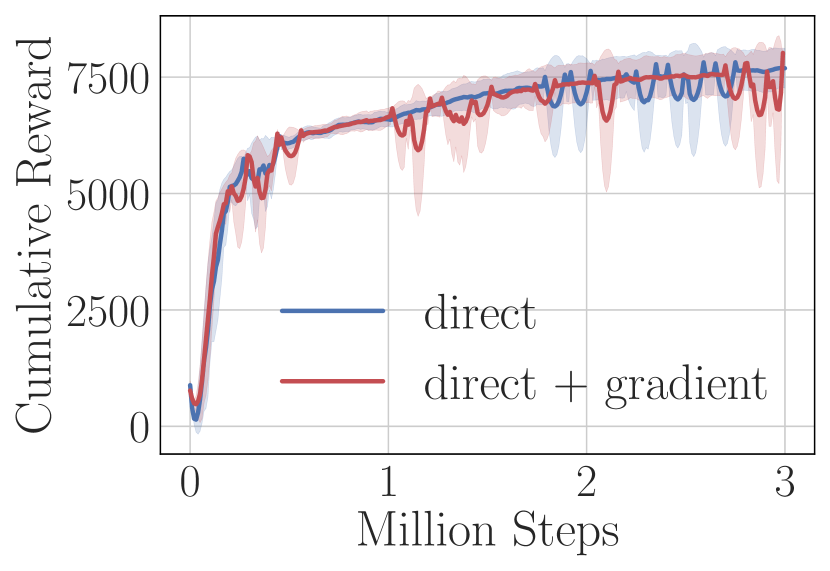
(d) Ant-v2

Figure 20: Test-Time Gradient-Based Optimization. Each plot compares the performance of direct amortization vs. direct amortization with $50$ additional gradient-based policy optimization iterations. Note that this additional optimization is only performed at test time.

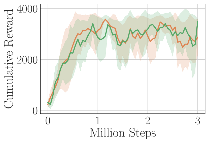
(a) Hopper-v2

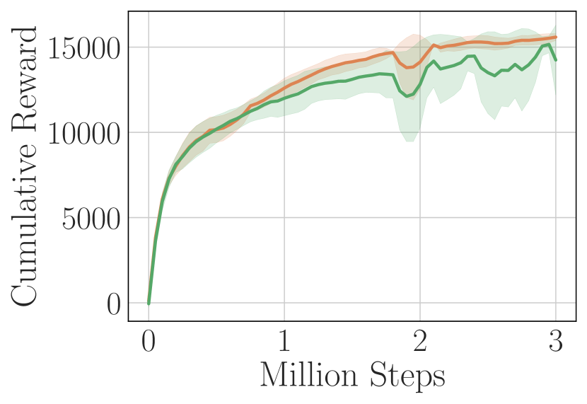
(b) HalfCheetah-v2

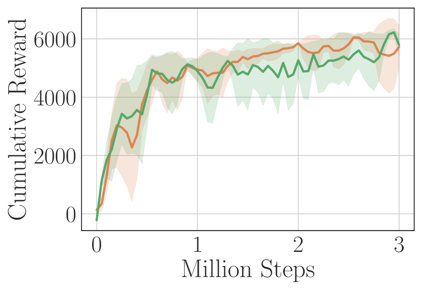
(c) Walker2d-v2

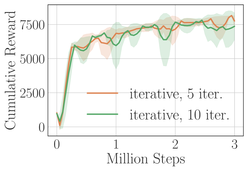
(d) Ant-v2

Figure 21: Additional Amortized Test-Time Iterations. Each plot compares the performance of iterative amortization (trained with $5$ iterations) vs. the same agent with an additional $5$ iterations at evaluation. Performance remains similar or slightly worse.

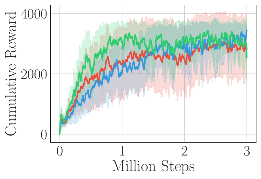
(a) Hopper-v2

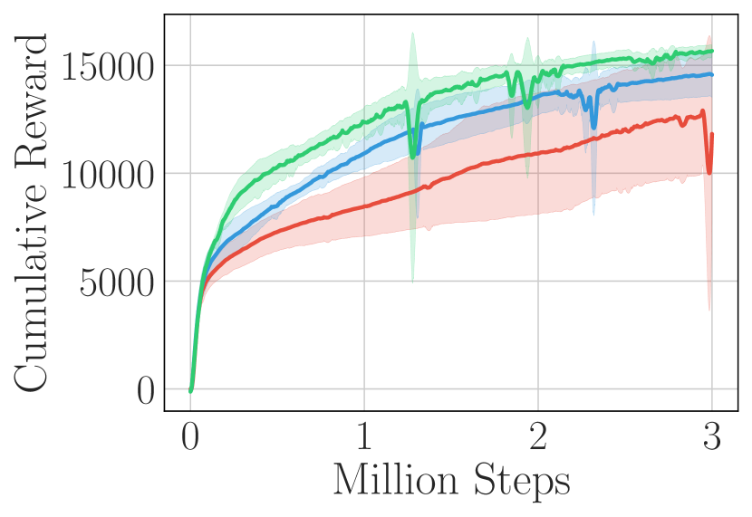
(b) HalfCheetah-v2

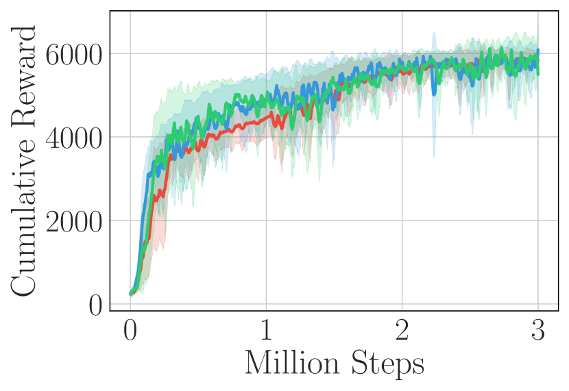
(c) Walker2d-v2

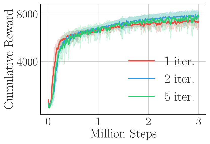
(d) Ant-v2

Figure 22: Performance of Varying Iterations During Training.

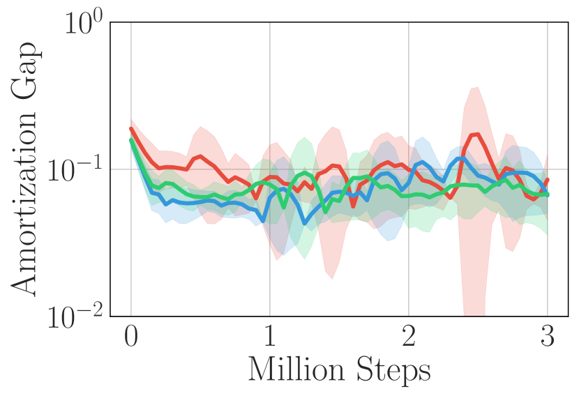
(a) Hopper-v2

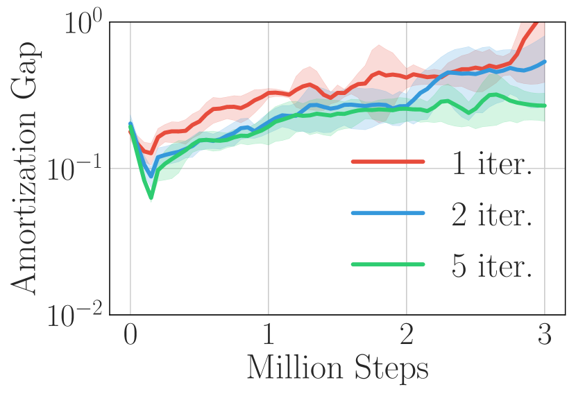
(b) HalfCheetah-v2

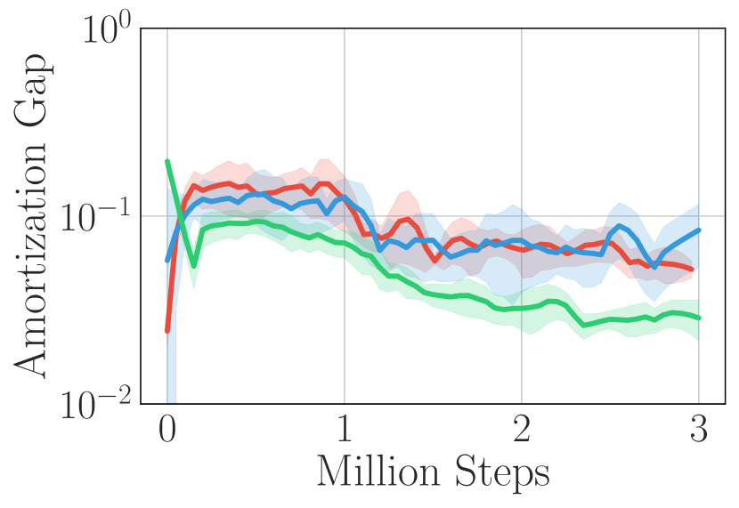
(c) Walker2d-v2

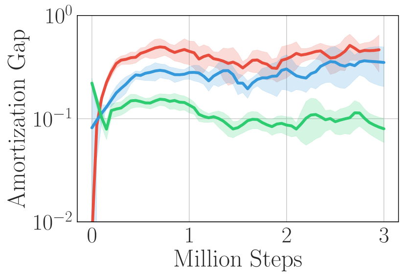
(d) Ant-v2

Figure 23: Amortization Gap of Varying Iterations During Training.

B.7 Multiple Policy Estimates

As discussed in Section 3.2, iterative amortization has the added benefit of potentially obtaining multiple policy distribution estimates, due to stochasticity in the optimization procedure as well as initialization. In contrast, unless latent variables are incorporated into the policy, direct amortization is limited to a single policy estimate. In Section 4.3.2, we analyzed multi-modality by comparing the distance between difference optimization runs of iterative amortization on Walker2d-v2. Here, we present the same analysis on each of the other three environments considered in this paper.

Again, we perform $10$ separate runs of policy optimization per state and evaluate the L2 distance between the means of these policy estimates after applying the tanh transform. Note that in MuJoCo action spaces, which are bounded to $[-1,1]$, the maximum distance is $2\sqrt{|\mathcal{A}|}$, where $|\mathcal{A}|$ is the size of the action space. We evaluate the policy mean distance over $100$ states and all $5$ experiment seeds. Results are shown in Figures 25, 24, and 26, where we plot (a) the histogram of distances between policy means ($\bm{\mu}$) across optimization runs ($i$ and $j$) over seeds and states at $3$ million environment steps, (b) the projected optimization surface on each pair of action dimensions for the state with the largest distance, and (c) the policy density for $10$ optimization runs. As before, we see that some subset of states retain multiple policy modes.

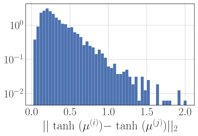
(a)

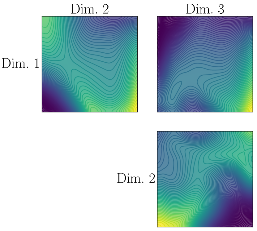
(b)

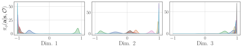
(c)

Figure 24: Multiple Policy Modes on Hopper-v2.

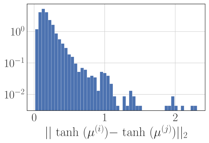
(a)

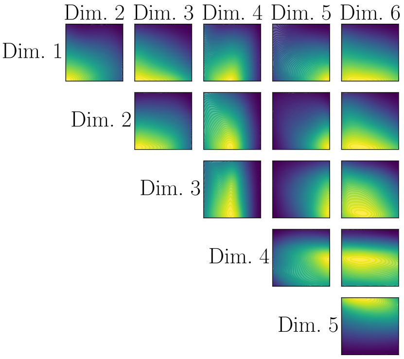
(b)

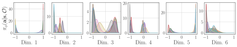
(c)

Figure 25: Multiple Policy Modes on HalfCheetah-v2.

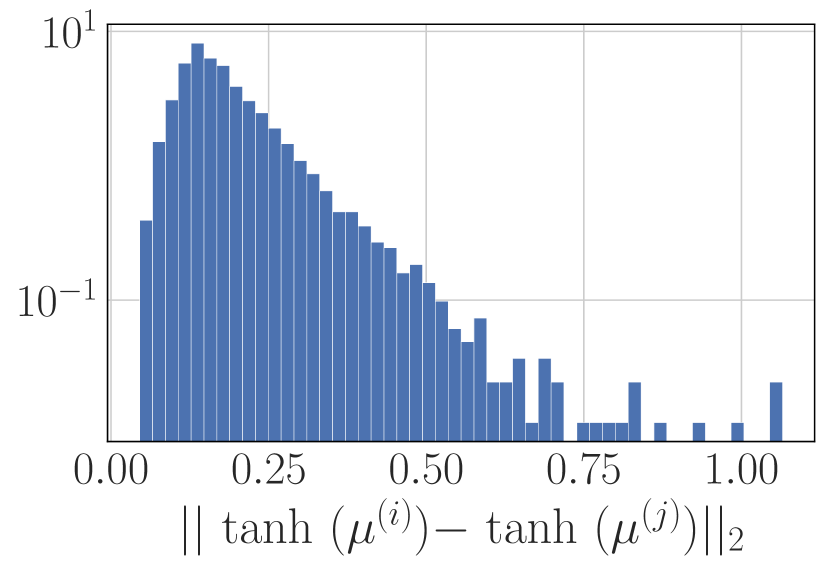
(a)

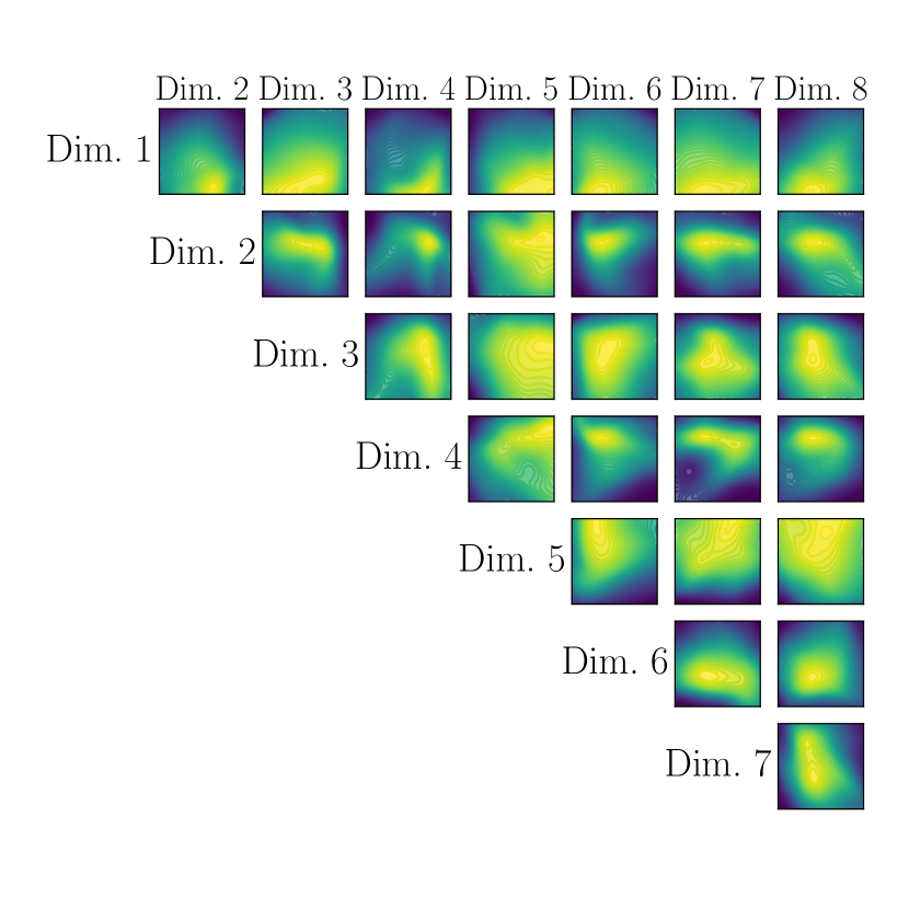
(b)

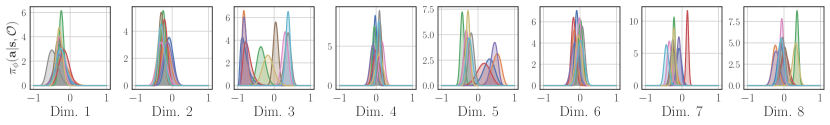
(c)

Figure 26: Multiple Policy Modes on Ant-v2.

References

- [1] Abbas Abdolmaleki, Jost Tobias Springenberg, Yuval Tassa, Remi Munos, Nicolas Heess, and Martin Riedmiller. Maximum a posteriori policy optimisation. In International Conference on Learning Representations, 2018.
- [2] Rishabh Agarwal, Dale Schuurmans, and Mohammad Norouzi. An optimistic perspective on offline reinforcement learning. In International Conference on Machine Learning, pages 104–114, 2020.
- [3] Zafarali Ahmed, Nicolas Le Roux, Mohammad Norouzi, and Dale Schuurmans. Understanding the impact of entropy on policy optimization. In International Conference on Machine Learning, pages 151–160, 2019.
- [4] Brandon Amos, Samuel Stanton, Denis Yarats, and Andrew Gordon Wilson. On the model-based stochastic value gradient for continuous reinforcement learning. In Learning for Dynamics and Control, pages 6–20. PMLR, 2021.
- [5] Brandon Amos and Denis Yarats. The differentiable cross-entropy method. In International Conference on Machine Learning, 2020.
- [6] Marcin Andrychowicz, Misha Denil, Sergio Gomez, Matthew W Hoffman, David Pfau, Tom Schaul, and Nando de Freitas. Learning to learn by gradient descent by gradient descent. In Advances in Neural Information Processing Systems, pages 3981–3989, 2016.
- [7] Karl Johan Astrom and Richard M Murray. Feedback Systems: An Introduction for Scientists and Engineers. Princeton University Press, 2008.
- [8] Hagai Attias. Planning by probabilistic inference. In AISTATS. Citeseer, 2003.
- [9] Jimmy Lei Ba, Jamie Ryan Kiros, and Geoffrey E Hinton. Layer normalization. NeurIPS Deep Learning Symposium, 2016.
- [10] Homanga Bharadhwaj, Kevin Xie, and Florian Shkurti. Model-predictive planning via cross-entropy and gradient-based optimization. In Learning for Dynamics and Control, pages 277–286, 2020.
- [11] Matthew Botvinick and Marc Toussaint. Planning as inference. Trends in cognitive sciences, 16(10):485–488, 2012.
- [12] Greg Brockman, Vicki Cheung, Ludwig Pettersson, Jonas Schneider, John Schulman, Jie Tang, and Wojciech Zaremba. Openai gym. arXiv preprint arXiv:1606.01540, 2016.
- [13] Arunkumar Byravan, Jost Tobias Springenberg, Abbas Abdolmaleki, Roland Hafner, Michael Neunert, Thomas Lampe, Noah Siegel, Nicolas Heess, and Martin Riedmiller. Imagined value gradients: Model-based policy optimization with tranferable latent dynamics models. In Conference on Robot Learning, pages 566–589, 2020.
- [14] Kurtland Chua, Roberto Calandra, Rowan McAllister, and Sergey Levine. Deep reinforcement learning in a handful of trials using probabilistic dynamics models. In Advances in Neural Information Processing Systems, pages 4754–4765, 2018.
- [15] Kamil Ciosek, Quan Vuong, Robert Loftin, and Katja Hofmann. Better exploration with optimistic actor critic. In Advances in Neural Information Processing Systems, pages 1787–1798, 2019.
- [16] Ignasi Clavera, Yao Fu, and Pieter Abbeel. Model-augmented actor-critic: Backpropagating through paths. In International Conference on Learning Representations, 2020.
- [17] Djork-Arné Clevert, Thomas Unterthiner, and Sepp Hochreiter. Fast and accurate deep network learning by exponential linear units (elus). In International Conference on Learning Representations, 2016.
- [18] Comet.ML. Comet.ML home page, 2021.
- [19] Gregory F Cooper. A method for using belief networks as influence diagrams. In Fourth Workshop on Uncertainty in Artificial Intelligence., 1988.
- [20] Chris Cremer, Xuechen Li, and David Duvenaud. Inference suboptimality in variational autoencoders. In International Conference on Machine Learning, pages 1078–1086, 2018.
- [21] Peter Dayan and Geoffrey E Hinton. Using expectation-maximization for reinforcement learning. Neural Computation, 9(2):271–278, 1997.
- [22] Roy Fox. Toward provably unbiased temporal-difference value estimation. Optimization Foundations for Reinforcement Learning Workshop at NeurIPS, 2019.
- [23] Roy Fox, Ari Pakman, and Naftali Tishby. Taming the noise in reinforcement learning via soft updates. In Proceedings of the Thirty-Second Conference on Uncertainty in Artificial Intelligence, pages 202–211. AUAI Press, 2016.
- [24] Scott Fujimoto, David Meger, and Doina Precup. Off-policy deep reinforcement learning without exploration. In International Conference on Machine Learning, pages 2052–2062, 2019.
- [25] Scott Fujimoto, Herke van Hoof, and David Meger. Addressing function approximation error in actor-critic methods. In International Conference on Machine Learning, pages 1587–1596, 2018.
- [26] Samuel Gershman and Noah Goodman. Amortized inference in probabilistic reasoning. In Proceedings of the Cognitive Science Society, volume 36, 2014.
- [27] Klaus Greff, Raphaël Lopez Kaufman, Rishabh Kabra, Nick Watters, Christopher Burgess, Daniel Zoran, Loic Matthey, Matthew Botvinick, and Alexander Lerchner. Multi-object representation learning with iterative variational inference. In International Conference on Machine Learning, pages 2424–2433, 2019.
- [28] Arthur Guez, Mehdi Mirza, Karol Gregor, Rishabh Kabra, Sebastien Racaniere, Theophane Weber, David Raposo, Adam Santoro, Laurent Orseau, Tom Eccles, et al. An investigation of model-free planning. In International Conference on Machine Learning, pages 2464–2473, 2019.
- [29] Tuomas Haarnoja, Kristian Hartikainen, Pieter Abbeel, and Sergey Levine. Latent space policies for hierarchical reinforcement learning. In International Conference on Machine Learning, pages 1851–1860, 2018.
- [30] Tuomas Haarnoja, Haoran Tang, Pieter Abbeel, and Sergey Levine. Reinforcement learning with deep energy-based policies. In International Conference on Machine Learning, pages 1352–1361. JMLR. org, 2017.
- [31] Tuomas Haarnoja, Aurick Zhou, Pieter Abbeel, and Sergey Levine. Soft actor-critic: Off-policy maximum entropy deep reinforcement learning with a stochastic actor. In International Conference on Machine Learning, pages 1856–1865, 2018.
- [32] Tuomas Haarnoja, Aurick Zhou, Kristian Hartikainen, George Tucker, Sehoon Ha, Jie Tan, Vikash Kumar, Henry Zhu, Abhishek Gupta, Pieter Abbeel, et al. Soft actor-critic algorithms and applications. arXiv preprint arXiv:1812.05905, 2018.
- [33] Danijar Hafner, Timothy Lillicrap, Ian Fischer, Ruben Villegas, David Ha, Honglak Lee, and James Davidson. Learning latent dynamics for planning from pixels. In International Conference on Machine Learning, pages 2555–2565. PMLR, 2019.
- [34] Charles R. Harris, K. Jarrod Millman, Stéfan J. van der Walt, Ralf Gommers, Pauli Virtanen, David Cournapeau, Eric Wieser, Julian Taylor, Sebastian Berg, Nathaniel J. Smith, Robert Kern, Matti Picus, Stephan Hoyer, Marten H. van Kerkwijk, Matthew Brett, Allan Haldane, Jaime Fernández del Río, Mark Wiebe, Pearu Peterson, Pierre Gérard-Marchant, Kevin Sheppard, Tyler Reddy, Warren Weckesser, Hameer Abbasi, Christoph Gohlke, and Travis E. Oliphant. Array programming with NumPy. Nature, 585(7825):357–362, September 2020.
- [35] Nicolas Heess, Gregory Wayne, David Silver, Timothy Lillicrap, Tom Erez, and Yuval Tassa. Learning continuous control policies by stochastic value gradients. In Advances in Neural Information Processing Systems, pages 2944–2952, 2015.
- [36] Mikael Henaff, William F Whitney, and Yann LeCun. Model-based planning with discrete and continuous actions. arXiv preprint arXiv:1705.07177, 2017.
- [37] Devon Hjelm, Ruslan R Salakhutdinov, Kyunghyun Cho, Nebojsa Jojic, Vince Calhoun, and Junyoung Chung. Iterative refinement of the approximate posterior for directed belief networks. In Advances in Neural Information Processing Systems, pages 4691–4699, 2016.
- [38] Sepp Hochreiter and Jürgen Schmidhuber. Long short-term memory. Neural computation, 9(8):1735–1780, 1997.
- [39] J. D. Hunter. Matplotlib: A 2d graphics environment. Computing in Science & Engineering, 9(3):90–95, 2007.
- [40] Michael Janner, Justin Fu, Marvin Zhang, and Sergey Levine. When to trust your model: Model-based policy optimization. In Advances in Neural Information Processing Systems, pages 12519–12530, 2019.
- [41] Dmitry Kalashnikov, Alex Irpan, Peter Pastor, Julian Ibarz, Alexander Herzog, Eric Jang, Deirdre Quillen, Ethan Holly, Mrinal Kalakrishnan, Vincent Vanhoucke, et al. Qt-opt: Scalable deep reinforcement learning for vision-based robotic manipulation. In Conference on Robot Learning, 2018.
- [42] Rudolph Emil Kalman. A new approach to linear filtering and prediction problems. Journal of Basic Engineering, 82(1):35–45, 1960.
- [43] Yoon Kim, Sam Wiseman, Andrew C Miller, David Sontag, and Alexander M Rush. Semi-amortized variational autoencoders. In International Conference on Machine Learning, 2018.
- [44] Diederik P Kingma and Max Welling. Stochastic gradient vb and the variational auto-encoder. In International Conference on Learning Representations, 2014.
- [45] Durk P Kingma and Jimmy Ba. Adam: A method for stochastic optimization. In International Conference on Learning Representations, 2015.
- [46] Durk P Kingma, Tim Salimans, Rafal Jozefowicz, Xi Chen, Ilya Sutskever, and Max Welling. Improved variational inference with inverse autoregressive flow. In Advances in Neural Information Processing Systems, pages 4743–4751, 2016.
- [47] Rahul G Krishnan, Dawen Liang, and Matthew Hoffman. On the challenges of learning with inference networks on sparse, high-dimensional data. In International Conference on Artificial Intelligence and Statistics, pages 143–151, 2018.
- [48] Aviral Kumar, Justin Fu, Matthew Soh, George Tucker, and Sergey Levine. Stabilizing off-policy q-learning via bootstrapping error reduction. In Advances in Neural Information Processing Systems, pages 11784–11794, 2019.
- [49] Aviral Kumar, Aurick Zhou, George Tucker, and Sergey Levine. Conservative q-learning for offline reinforcement learning. In Advances in Neural Information Processing Systems, pages 1179–1191, 2020.
- [50] Keuntaek Lee, Kamil Saigol, and Evangelos A Theodorou. Safe end-to-end imitation learning for model predictive control. In International Conference on Robotics and Automation, 2019.
- [51] Sergey Levine. Reinforcement learning and control as probabilistic inference: Tutorial and review. arXiv preprint arXiv:1805.00909, 2018.
- [52] Timothy P Lillicrap, Jonathan J Hunt, Alexander Pritzel, Nicolas Heess, Tom Erez, Yuval Tassa, David Silver, and Daan Wierstra. Continuous control with deep reinforcement learning. In International Conference on Learning Representations, 2016.
- [53] Long-Ji Lin. Self-improving reactive agents based on reinforcement learning, planning and teaching. Machine learning, 8(3-4):293–321, 1992.
- [54] Joseph Marino, Milan Cvitkovic, and Yisong Yue. A general method for amortizing variational filtering. In Advances in Neural Information Processing Systems, 2018.
- [55] Joseph Marino, Yisong Yue, and Stephan Mandt. Iterative amortized inference. In International Conference on Machine Learning, pages 3403–3412, 2018.
- [56] Andriy Mnih and Karol Gregor. Neural variational inference and learning in belief networks. In International Conference on Machine Learning, pages 1791–1799, 2014.
- [57] Volodymyr Mnih, Adria Puigdomenech Badia, Mehdi Mirza, Alex Graves, Timothy Lillicrap, Tim Harley, David Silver, and Koray Kavukcuoglu. Asynchronous methods for deep reinforcement learning. In International Conference on Machine Learning, pages 1928–1937, 2016.
- [58] Volodymyr Mnih, Koray Kavukcuoglu, David Silver, Alex Graves, Ioannis Antonoglou, Daan Wierstra, and Martin Riedmiller. Playing atari with deep reinforcement learning. In NeurIPS Deep Learning Workshop, 2013.
- [59] Rémi Munos, Tom Stepleton, Anna Harutyunyan, and Marc Bellemare. Safe and efficient off-policy reinforcement learning. In Advances in Neural Information Processing Systems, pages 1054–1062, 2016.
- [60] Anusha Nagabandi, Gregory Kahn, Ronald S Fearing, and Sergey Levine. Neural network dynamics for model-based deep reinforcement learning with model-free fine-tuning. In International Conference on Robotics and Automation, pages 7559–7566. IEEE, 2018.
- [61] Adam Paszke, Sam Gross, Francisco Massa, Adam Lerer, James Bradbury, Gregory Chanan, Trevor Killeen, Zeming Lin, Natalia Gimelshein, Luca Antiga, et al. Pytorch: An imperative style, high-performance deep learning library. Advances in Neural Information Processing Systems, pages 8026–8037, 2019.
- [62] Alexandre Piché, Valentin Thomas, Cyril Ibrahim, Yoshua Bengio, and Chris Pal. Probabilistic planning with sequential monte carlo methods. In International Conference on Learning Representations, 2019.
- [63] Aravind Rajeswaran, Igor Mordatch, and Vikash Kumar. A game theoretic framework for model based reinforcement learning. In International Conference on Machine Learning, pages 7953–7963, 2020.
- [64] Danilo Jimenez Rezende, Shakir Mohamed, and Daan Wierstra. Stochastic backpropagation and approximate inference in deep generative models. In International Conference on Machine Learning, pages 1278–1286, 2014.
- [65] Benjamin Rivière, Wolfgang Hönig, Yisong Yue, and Soon-Jo Chung. Glas: Global-to-local safe autonomy synthesis for multi-robot motion planning with end-to-end learning. IEEE Robotics and Automation Letters, 5(3):4249–4256, 2020.
- [66] Reuven Y Rubinstein and Dirk P Kroese. The cross-entropy method: a unified approach to combinatorial optimization, Monte-Carlo simulation and machine learning. Springer Science & Business Media, 2013.
- [67] John Schulman, Sergey Levine, Pieter Abbeel, Michael Jordan, and Philipp Moritz. Trust region policy optimization. In International Conference on Machine Learning, pages 1889–1897, 2015.
- [68] John Schulman, Filip Wolski, Prafulla Dhariwal, Alec Radford, and Oleg Klimov. Proximal policy optimization algorithms. arXiv preprint arXiv:1707.06347, 2017.
- [69] David Silver, Aja Huang, Chris J Maddison, Arthur Guez, Laurent Sifre, George Van Den Driessche, Julian Schrittwieser, Ioannis Antonoglou, Veda Panneershelvam, Marc Lanctot, et al. Mastering the game of go with deep neural networks and tree search. Nature, 529(7587):484–489, 2016.
- [70] David Silver, Guy Lever, Nicolas Heess, Thomas Degris, Daan Wierstra, and Martin Riedmiller. Deterministic policy gradient algorithms. In International Conference on Machine Learning, pages 387–395, 2014.
- [71] Aravind Srinivas, Allan Jabri, Pieter Abbeel, Sergey Levine, and Chelsea Finn. Universal planning networks: Learning generalizable representations for visuomotor control. In International Conference on Machine Learning, pages 4732–4741, 2018.
- [72] Rupesh K Srivastava, Klaus Greff, and Jürgen Schmidhuber. Training very deep networks. In Advances in Neural Information Processing Systems, pages 2377–2385, 2015.
- [73] Richard S Sutton and Andrew G Barto. Reinforcement learning: An introduction. MIT press, 2018.
- [74] Yunhao Tang and Shipra Agrawal. Boosting trust region policy optimization by normalizing flows policy. In NeurIPS Deep Reinforcement Learning Workshop, 2018.
- [75] Sebastian Thrun and Anton Schwartz. Issues in using function approximation for reinforcement learning. In Proceedings of the 1993 Connectionist Models Summer School Hillsdale, NJ. Lawrence Erlbaum, 1993.
- [76] Dhruva Tirumala, Hyeonwoo Noh, Alexandre Galashov, Leonard Hasenclever, Arun Ahuja, Greg Wayne, Razvan Pascanu, Yee Whye Teh, and Nicolas Heess. Exploiting hierarchy for learning and transfer in kl-regularized rl. arXiv preprint arXiv:1903.07438, 2019.
- [77] Emanuel Todorov. General duality between optimal control and estimation. In Decision and Control, 2008. CDC 2008. 47th IEEE Conference on, pages 4286–4292. IEEE, 2008.
- [78] Emanuel Todorov, Tom Erez, and Yuval Tassa. Mujoco: A physics engine for model-based control. In International Conference on Intelligent Robots and Systems, pages 5026–5033. IEEE, 2012.
- [79] Marc Toussaint and Amos Storkey. Probabilistic inference for solving discrete and continuous state markov decision processes. In International Conference on Machine Learning, pages 945–952, 2006.
- [80] Hado Van Hasselt. Double q-learning. In Advances in Neural Information Processing Systems, pages 2613–2621, 2010.
- [81] Hado Van Hasselt, Arthur Guez, and David Silver. Deep reinforcement learning with double q-learning. In AAAI Conference on Artificial Intelligence, 2016.
- [82] Michael L. Waskom. seaborn: statistical data visualization. Journal of Open Source Software, 6(60):3021, 2021.
- [83] Ronald J Williams. Simple statistical gradient-following algorithms for connectionist reinforcement learning. In Reinforcement Learning, pages 5–32. Springer, 1992.
- [84] Yifan Wu, George Tucker, and Ofir Nachum. Behavior regularized offline reinforcement learning. arXiv preprint arXiv:1911.11361, 2019.