Reinforcement Learning for Optimization of COVID-19 Mitigation Policies

Abstract

The year 2020 has seen the covid-19 virus lead to one of the worst global pandemics in history. As a result, governments around the world are faced with the challenge of protecting public health, while keeping the economy running to the greatest extent possible. Epidemiological models provide insight into the spread of these types of diseases and predict the effects of possible intervention policies. However, to date, the even the most data-driven intervention policies rely on heuristics. In this paper, we study how reinforcement learning (RL) can be used to optimize mitigation policies that minimize the economic impact without overwhelming the hospital capacity. Our main contributions are (1) a novel agent-based pandemic simulator which, unlike traditional models, is able to model fine-grained interactions among people at specific locations in a community; and (2) an RL-based methodology for optimizing fine-grained mitigation policies within this simulator. Our results validate both the overall simulator behavior and the learned policies under realistic conditions.

1 Introduction

Motivated by the devastating covid-19 pandemic, much of the scientific community, across numerous disciplines, is currently focused on developing safe, quick, and effective methods to prevent the spread of biological viruses, or to otherwise mitigate the harm they cause. These methods include vaccines, treatments, public policy measures, economic stimuli, and hygiene education campaigns. Governments around the world are now faced with high-stakes decisions regarding which measures to enact at which times, often involving trade-offs between public health and economic resiliency. When making these decisions, governments often rely on epidemiological models that predict and project the course of the pandemic.

The premise of this paper is that the challenge of mitigating the spread of a pandemic while maximizing personal freedom and economic activity is fundamentally a sequential decision-making problem: the measures enacted on one day affect the challenges to be addressed on future days. As such, modern reinforcement learning (RL) algorithms are well-suited to optimize government responses to pandemics.

For such learned policies to be relevant, they must be trained within an epidemiological model that accurately simulates the spread of the pandemic, as well as the effects of government measures. To the best of our knowledge, none of the existing epidemiological simulations have the resolution to allow reinforcement learning to explore the regulations that governments are currently struggling with.

Motivated by this, our main contributions are:

1. The introduction of PandemicSimulator, a novel open-source agent-based simulator that models the interactions between individuals at specific locations within a community. Developed in collaboration between AI researchers and epidemiologists (the co-authors of this paper), PandemicSimulator models realistic effects such as testing with false positive/negative rates, imperfect public adherence to social distancing measures, contact tracing, and variable spread rates among infected individuals. Crucially, PandemicSimulator models community interactions at a level of detail that allows the spread of the disease to be an emergent property of people’s behaviors and the government’s policies. An interface with OpenAI Gym (Brockman et al. 2016) is provided to enable support for standard RL libraries;

2. A demonstration that a reinforcement learning algorithm can indeed identify a policy that outperforms a range of reasonable baselines within this simulator;

3. An analysis of the resulting learned policy, which may provide insights regarding the relative efficacy of past and potential future covid-19 mitigation policies.

While the resulting policies have not been implemented in any real-world communities, this paper establishes the potential power of RL in an agent-based simulator, and may serve as an important first step towards real-world adoption.

The remainder of the paper is organized as follows. We first discuss related work and then introduce our simulator in Section 3. Section 4 presents our reinforcement learning setup, while results are reported in Section 5. Finally, Section 6 reports some conclusions and directions for future work.

2 Related Work

Epidemiological models differ based on the level of granularity in which they track individuals and their disease states. “Compartmental” models group individuals of similar disease states together, assume all individuals within a specific compartment to be homogeneous, and only track the flow of individuals between compartments (Tolles and Luong 2020). While relatively simplistic, these models have been used for decades and continue to be useful for both retrospective studies and forecasts as were seen during the emergence of recent diseases (Rivers and Scarpino 2018; Metcalf and Lessler 2017; Cobey 2020).

However, the commonly used macroscopic (or mass-action) compartmental models are not appropriate when outcomes depend on the characteristics of heterogeneous individuals. In such cases, network models (Bansal, Grenfell, and Meyers 2007; Liu et al. 2018; Khadilkar, Ganu, and Seetharam 2020) and agent-based models (Grefenstette et al. 2013; Del Valle, Mniszewski, and Hyman 2013; Aleta et al. 2020) may be more useful predictors. Network models encode the relationships between individuals as static connections in a contact graph along which the disease can propagate. Conversely, agent-based simulations, such as the one introduced in this paper, explicitly track individuals, their current disease states, and their interactions with other agents over time. Agent-based models allow one to model as much complexity as desired—even to the level of simulating individual people and locations as we do—and thus enable one to model people’s interactions at offices, stores, schools, etc. Because of their increased detail, they enable one to study the hyper-local interventions that governments consider when setting policy. For instance, Larremore et al. (2020) simulate the SARS-CoV-2 dynamics both through a fully-mixed mass-action model and an agent-based model representing the population and contact structure of New York City.

PandemicSimulator has the level of details needed to allow us to apply RL to optimize dynamic government intervention policies (sometimes referred to as “trigger analysis” e.g. Duque et al. 2020). RL has been applied previously to several mass-action models (Libin et al. 2020; Song et al. 2020). These models, however, do not take into account individual behaviors or any complex interaction patterns. The work that is most closely related to our own includes both the SARS-CoV-2 epidemic simulators from Hoertel et al. (2020) and Aleta et al. (2020), which model individuals grouped into households who visit and interact in the community. While their approach builds accurate contact networks of real populations, it doesn’t allow us to model how the contact network would change as the government intervenes. Xiao et al. (2020) construct a detailed, pedestrian level simulation that simulates transmission indoors and study three types of interventions. Liu (2020) presents a microscopic approach to model epidemics, which can explicitly consider the consequences of individuals’ decisions on the spread of the disease. Multi-agent RL is then used to let individual agents learn to avoid infections.

For any model to be accepted by real-world decision-makers, they must be provided with a reason to trust that it accurately models the population and spread dynamics in their own community. For both mass-action and agent-based models, this trust is typically best instilled via a model calibration process that ensures that the model accurately tracks past data. For example, Hoertel et al. (2020) perform a calibration using daily mortality data until 15 April. Similarly, Libin et al. (2020) calibrate their model based on the symptomatic cases reported by the British Health Protection Agency for the 2009 influenza pandemic. Aleta et al. (2020), instead, only calibrate the weights of intra-layer links by means of a rescaling factor, such that the mean number of daily effective contacts in that layer matches mean number of daily effective contacts in the corresponding social setting. While not a main focus of our research, we have taken initial steps to demonstrate that our model can be calibrated to track real-world data, as described in Section 3.

3 PandemicSimulator: A COVID-19 Simulator

The functional blocks of PandemicSimulator, shown in Figure 1, are:

• locations, with properties that define how people interact within them;

• people, who travel from one location to another according to individual daily schedules;

• an infection model that updates the infection state of each person;

• an optional testing strategy that imperfectly exposes the infection state of the population;

• an optional contact tracing strategy that identifies an infected person’s recent contacts;

• a government that makes policy decisions.

The simulator models a day as 24 discrete hours, with each person potentially changing locations each hour. At the end of a day, each person’s infection state is updated. The government interacts with the environment by declaring regulations, which impose restrictions on the people and locations. If the government activates testing, the simulator identifies a set of people to be tested and (imperfectly) reports their infection state. If contact tracing is active, each person’s contacts from the previous days are updated. The updated perceived infection state and other state variables are returned as an observation to the government. The process iterates as long as the infection remains active.

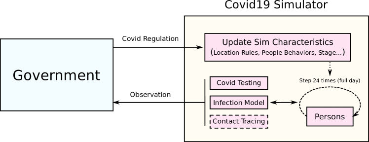
Figure 1: Block diagram of the simulator.

The following subsections describe the functional blocks of the simulator in greater detail.

Locations

Each location has a set of attributes that specify when the location is open, what roles people play there (e.g. worker or visitor), and the maximum number of people of each role. These attributes can be adjusted by regulations, such as when the government determines that businesses should operate at half capacity. Non-essential locations can be completely closed by the government. The location types used in our experiments are homes, hospitals, schools, grocery stores, retail stores, and hair salons. The simulator provides interfaces to make it easy to add new location types.

One of the advantages of an agent-based approach is that we can more accurately model variations in the way people interact in different types of locations based on their roles. The base location class supports workers and visitors, and defines a contact rate, $b^{\text{loc}}$, as a 3-tuple $(x,y,z)\in[0,1]^{3}$, where $x$ is the worker-worker rate, $y$ is the worker-visitor rate, and $z$ is the visitor-visitor rate. These rates are used to sample interactions every hour in each location to compute disease transmissions. For example, consider a location that has a contact rate of $(0.5,0.3,0.4)$ and 10 workers and 20 visitors. In expectation, a worker would make contact with 5 co-workers and 6 visitors in the given hour. Similarly, a visitor would be expected to make contact with 3 workers and 8 other visitors. Refer to our supplementary material (Appendix A, Table 1) for a listing of the contact rates and other parameters for all location types used in our experiments.

The base location type can be extended for more complex situations. For example, a hospital adds an additional role (critically sick patients), a capacity representing ICU beds, and contact rates between workers and patients.

Population

A person in the simulator is an automaton that has a state and a person-specific behavior routine. These routines create person-to-person interactions throughout the simulated day and induce dynamic contact networks.

Individuals are assigned an age, drawn from the distribution of the US age demographics, and are randomly assigned to be either high risk or of normal health. Based on their age, each person is categorized as either a minor, a working adult or a retiree. Working adults are assigned to a work location, and minors to a school, which they attend 8 hours a day, five days a week. Adults and retirees are assigned favorite hair salons which they visit once a month, and grocery and retail stores which they visit once a week. Each person has a compliance parameter that determines the probability that the person flouts regulations each hour.

The simulator constructs households from this population such that $15\%$ house only retirees, and the rest have at least one working adult and are filled by randomly assigning the remaining children, adults, and retirees. To simulate informal social interactions, households may attend social events twice a month, subject to limits on gathering sizes.

At the end of each simulated day, the person’s infection state is updated through a stochastic model based on all of that individual’s interactions during the day (see next section). Unless otherwise prescribed by the government, when a person becomes ill they follow their routine. However, even the most basic government interventions require sick people to stay home, and at-risk individuals to avoid large gatherings. If a person becomes critically ill, they are admitted to the hospital, assuming it has not reached capacity.

SEIR Infection Model

PandemicSimulator implements a modified SEIR (susceptible, exposed, infected, recovered) infection model, as shown in Figure 2. See supplemental Appendix A, Table 2 for specific parameter values and the transition probabilities of the SEIR model. Once exposed to the virus, an individual’s path through the disease is governed by the transition probabilities. However, the transition from the susceptible state ($S$) to the exposed state $(E)$ requires a more detailed explanation.

At the beginning of the simulation, a small, randomly selected set of individuals seeds the pandemic in the latent non-infectious, exposed state ($E$). The rest of the population starts in $S$. The exposed individuals soon transition to one of the infectious states and start interacting with susceptible people. For each susceptible person $i$, the probability they become infected on a given day, $P^{S\rightarrow E}_{i}(\textit{day})$, is calculated based on their contacts with infectious people that day.

$$P^{S\rightarrow E}_{i}(\textit{day})=1-\prod_{t=0}^{23}\overline{P}^{S\rightarrow E}_{i}(t)$$ (1)

where $\overline{P}^{S\rightarrow E}_{i}(t)$ is the probability that person $i$ is not infected at hour $t$. Whether a susceptible person becomes infected in a given hour depends on whom they come in contact with. Let $\mathcal{C}^{j}_{i}(t)=\{\textit{p}\overset{b^{j}}{\sim}N_{j}(t)|\textit{p}\in N^{\text{inf}}_{j}(t)\}$ be the set of infected contacts of person $i$ in location $j$ at hour $t$ where $N^{\text{inf}}_{j}(t)$ is the set of infected persons in location $j$ at time $t$, $N_{j}(t)$ is the set of all persons in $j$ at time $t$, and $b^{j}$ is a hand-set contact rate for $j$. To model the variations in how easily individuals spread the disease, each individual $k$ has an infection spread rate, $a^{k}\sim\mathcal{N}^{\text{bounded}}(a,\sigma)$ sampled from a bounded Gaussian distribution. Accordingly,

$$\overline{P}^{S\rightarrow E}_{i}(t)=\prod_{k\in\mathcal{C}^{j}_{i}(t)}(1-a^{k}).$$ (2)

Figure 2: SEIR model used in PandemicSimulator

Testing and Contact Tracing

PandemicSimulator features a testing procedure to identify positive cases of covid-19. We do not model concomitant illnesses, so every critically sick or dead person is assumed to have tested positive. Non-symptomatic and symptomatic individuals—and individuals that previously tested positive—get tested all at different configurable rates. Additionally, we model false positive and false negative test results. Refer to the supplementary material (Appendix A, Table 1) for a listing of the testing rates used in our experiment.

The government can also implement a contact tracing strategy that tracks, over the last $N$ days, the number of times each pair of individuals interacted. When activated, this procedure allows the government to test or quarantine all recent 1^st-order contacts and their households when an individual tests positive for covid-19.

Government Regulations

As discussed earlier (see Figure 1), the government announces regulations to try to control the pandemic. The government can impose the following rules:

• social distancing: a value $\beta\in[0,1]$ that scales the contact rates of each location by $(1-\beta)$. 0 corresponds to unrestricted interactions; 1 eliminates all interactions;

• stay home if sick: a boolean. When set, people who have tested positive are requested to stay at home;

• practice good hygiene: a boolean. When set, people are requested to practice better-than-usual hygiene.

• wear facial coverings: a boolean. When set, people are instructed to wear facial coverings.

• avoid gatherings: a value that indicates the maximum recommended size of gatherings. These values can differ for high risk individuals and those of normal health;

• closed businesses: A list of non-essential business location types that are not permitted to open.

These types of regulations, modeled after government policies seen throughout the world, are often bundled into progressive stages to make them easier to communicate to the population. Refer to Appendix A, Tables 1-3 for details on the parameters, their sources and the values set for each stage.

Calibration

PandemicSimulator includes many parameters whose values are still poorly known, such as the spread rate of covid-19 in grocery stores and the degree to which face masks reduce transmission. We therefore consider these parameters as free variables that can be used to calibrate the simulator to match the historical data that has been observed around the world. These parameters can also be used to customize the simulator to match a specific community. A discussion of our calibration process and the values we chose to model covid-19 are discussed in Appendix A.

4 RL for Optimization of Regulations

An ideal solution to minimize the spread of a new disease like covid-19 is to eliminate all non-essential interactions and quarantine infected people until the last infected person has recovered. However, the window to execute this policy with minimal economic impact is very small. Once the disease spreads widely this policy becomes impractical and the potential negative impact on the economy becomes enormous. In practice, around the world we have seen a strict lockdown followed by a gradual reopening that attempts to minimize the growth of the infection while allowing partial economic activity. Because covid-19 is highly contagious, has a long incubation period, and large portions of the infected population are asymptomatic, managing the reopening without overwhelming healthcare resources is challenging. In this section, we tackle this sequential decision making problem using reinforcement learning (RL; Sutton and Barto 2018) to optimize the reopening policy.

To define an RL problem we need to specify the environment, observations, actions, and rewards.

Environment:

The agent-based pandemic simulator PandemicSimulator is the environment.

Actions:

The government is the learning agent. Its goal is to maximize its reward over the horizon of the pandemic. Its action set is constrained to a pool of escalating stages, which it can either increase, decrease, or keep the same when it takes an action. Refer to Appendix A, Table 3 for detailed descriptions of the stages.

Observations:

At the end of each simulated day, the government observes the environment. For the sake of realism, the infection status of the population is partially observable, accessible only via statistics reflecting aggregate (noisy) test results and number of hospitalizations.

Rewards:

We designed our reward function to encourage the agent to keep the number of persons in critical condition ($n^{c}$) below the hospital’s capacity ($C^{\text{max}}$), while keeping the economy as unrestricted as possible. To this end, we use a reward that is a weighted sum of two objectives:

$$r=a~{}\max\left(\frac{n^{c}-C^{\text{max}}}{C^{\text{max}}},~{}0\right)+b~{}\frac{\text{stage}^{p}}{\max_{j}\text{stage}^{p}_{j}}$$ (3)

where $\text{stage}\in[0,4]$ denotes one of the 5 stages with $\text{stage}_{4}$ being the most restrictive. $a$, $b$ and $p$ are set to $-0.4$, $-0.1$ and $1.5$, respectively, in our experiments. To discourage frequently changing restrictions, we also use a small shaping reward (with $-0.02$ coefficient) proportional to $|stage(t-1)-stage(t)|$. This linear mapping of stages into a $[0,1]$ reward space is arbitrary; if PandemicSimulator were being used to make real policy decisions, policy makers would use values that represent the real economic costs of the different stages.

Training:

We use the discrete-action Soft Actor Critic (SAC;  Haarnoja et al. 2018) off-policy RL algorithm to optimize a reopening policy, where the actor and critic networks are two-layer deep multi-layer perceptrons with 128 hidden units. One motivation behind using SAC over deep Q-learning approaches such as DQN (Mnih et al. 2015) is that we can provide the true infection summary as inputs to the critic while letting the actor see only the observed infection summary. Training is episodic with each episode lasting 120 simulated days. At the end of each episode, the environment is reset to an initial state. Refer to Appendix A, Table 1 for learning parameters.

5 Experiments

Figure 3: A single run of the simulator with no government restrictions, showing (a) the true global infection summary (b) the perceived infection state, and (c) the number of people in critical condition over time.

Figure 4: Simulator dynamics at different regulation stages. The plots are generated based on 30 different randomly seeded runs of the simulator. Mean is shown by a solid line and variance either by a shaded region or an error line. In the left set of graphs, the red line at the top indicates what regulation stage is in effect on any given day.

The purpose of PandemicSimulator is to enable a more realistic evaluation of potential government policies for pandemic mitigation. In this section, we validate that the simulation behaves as expected under controlled conditions, illustrate some of the many analyses it facilitates, and most importantly, demonstrate that it enables optimization via RL.

Unless otherwise specified, we consider a community size of 1,000 and a hospital capacity of 10. To enable calibration with real data, we limit government actions to five regulation stages similar to those used by real-world cities (see appendix for details), and assume the government does not act until at least five people are infected.

Figure 3 shows plots of a single simulation run with no government regulations (Stage 0). Figure 3(a) shows the number of people in each infection category per day. Without government intervention, all individuals get infected, with the infection peaking around the $25^{\text{th}}$ day. Figure 3(b) shows the metrics observed by the government through the lens of testing and hospitalizations. This plot illustrates how the government sees information that is both an underestimate of the penetration and delayed in time from the true state. Finally, Figure 3(c) shows that the number of people in critical condition goes well above the maximum hospital capacity (denoted with a yellow line) resulting in many people being more likely to die. The goal of a good reopening policy is to keep the red curve below the yellow line, while keeping as many businesses open as possible.

Figure 4 shows plots of our infection metrics averaged over 30 randomly seeded runs. Each row in Figures 4(a-o) shows the results of executing a different (constant) regulation stage (after a short initial S0 phase), where S4 is the most restrictive and S0 is no restrictions. As expected, Figures 4(p-r) show that the infection peaks, critical cases and number of deaths are all lower for more restrictive stages. One way of explaining the effects of these regulations is that the government restrictions alter the connectivity of the contact graph. For example, in the experiments above, under stage 4 restrictions there are many more connected components in the resulting contact graph than in any of the other 4 cases. See Appendix A for details of this analysis.

Higher stage restrictions, however, have increased socio-economic costs (Figure 4(s); computed using the second objective in Eq. 3). Our RL experiments illustrate how these competing objectives can be balanced.

A key benefit of PandemicSimulator’s agent-based approach is that it enables us to evaluate more dynamic policies than those described above. In the remainder of this section we compare a set of hand constructed policies, examine (approximations) of two real country’s policies, and study the impact of contact tracing. In Appendix A we also provide an analysis of the model’s sensitivity to its parameters. Finally, we demonstrate the application of RL to construct dynamic polices that achieve the goal of avoiding exceeding hospital capacity while minimizing economic costs. As in Figure 4, throughout this section we report our results using plots that are generated by executing 30 simulator runs with fixed seeds. All our experiments were run on a single core, using an Intel i7-7700K CPU $@$ 4.2GHz with 32GB of RAM.

Benchmark Policies

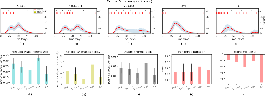
Figure 5: Simulator dynamics under different hand constructed and reference government policies.

Figure 6: Simulator runs comparing the S0-4-0-GI heuristic policy with a learned policy. The figure also shows results of the learned policy evaluated at different action frequencies and in a larger population environment.

To serve as benchmarks, we defined three heuristic and two policies inspired by real governments’ approaches to managing the pandemic.

• S0-4-0: Using this policy, the government switches from stage 0 to 4 after reaching a threshold of 10 infected persons. After 30 days, it switches directly back to stage 0;

• S0-4-0-FI: The government starts like S0-4-0, but after 30 days it executes a fast, incremental (FI) return to stage 0, with intermediate stages lasting 5 days;

• S0-4-0-GI: This policy implements a more gradual incremental (GI) return to stage 0, with each intermediate stage lasting 10 days;

• SWE: This policy represents the one adopted by the Swedish government, which recommended, but did not require remote work, and was generally unrestrictive. Table 4 in the supplementary material shows how we mapped this policy into a 2-stage action space.

• ITA: this policy represents the one adopted by the Italian government, which was generally much more restrictive. Table 5 shows our mapping of this policy to a 5-stage action space.

Figure 5 compares the hand constructed policies. From the point of view of minimizing overall mortality, S0-4-0-GI performed best. In particular, slower re-openings ensure longer but smaller peaks. While this approach leads to a second wave right after stage 0 is reached, the gradual policy prevents hospital capacity from being exceeded.

Figure 5 also contrasts the approximations of the policies employed by Sweden and Italy in the early stages of the pandemic (through February 2020). The ITA policy leads to fewer deaths and only a marginally longer duration. However, this simple comparison does not account for the economic cost of policies, an important factor that is considered by decision-makers.

Testing and Contact Tracing

To validate PandemicSimulator’s ability to model testing and contact tracing we compare several strategies with different testing rates and contact horizons. We consider daily testing rates of 0.02, 0.3, and 1.0 (where 1.0 represents the extreme case of everyone being tested every day) and contact tracing histories of 0, 2, 5, or 10 days. For each condition, we ran the experiments with the same 30 random seeds. The full results appear in Appendix A.

Not surprisingly, contact tracing is most beneficial with higher testing rates and longer contact histories because more testing finds more infected people and the contact tracing is able to encourage more of that person’s contacts to stay home. Of course, the best strategy is to test every person every day and quarantine anyone who tests positive. Unfortunately, this strategy is impractical except in the most isolated communities. Although this aggressive strategy often stamps out the disease, the false-negative test results sometimes allow the infection to simmer below the surface and spread very slowly through the population.

Optimizing Reopening using RL

A major design goal of PandemicSimulator is to support optimization of re-opening policies using RL. In this section, we test our hypothesis that a learned policy can outperform the benchmark policies. Specifically, RL optimizes a policy that (a) is adaptive to the changing infection state, (b) keeps the number of critical patients below the hospital threshold, and (c) minimizes the economic cost.

We ran experiments using the 5-stage regulations defined in Table 3 (Appendix A); trained the policy by running RL optimization for roughly 1 million training steps; and evaluated the learned policies across 30 randomly seeded initial conditions. Figures 6(a-f) show results comparing our best heuristic policy (S0-4-0-GI) to the learned policy. The learned policy is better across all metrics as shown in Figures 6(m-p). Further, we can see how the learned policy reacts to the state of the pandemic; Figure 6(f) shows different traces through the regulation space for 3 of the trials. The learned policy briefly oscillates between Stages 3 and 4 around day $40$. To minimize such oscillations, we evaluated the policy at an action frequency of one action every 3 days (bi-weekly; labeled as Eval_w3) and every 7 days (weekly; labeled as Eval_w7). Figure 6(p) shows that the bi-weekly variant performs well, while making changes only once a week slightly reduces the reward. To test robustness to scaling, we also evaluated the learned policy (with daily actions) in a town with a population of 10,000 (Eval_10k) and found that the results transfer well. This success hints at the possibility of learning policies quickly even when intending to transfer them to large cities.

This section presented results on applying RL to optimize reopening policies. An interesting next step would be to study and explain the learned policies as simpler rule based strategies to make it easier for policy makers to implement. For example, in Figure 6(l), we see that the RL policy waits at stage 2 before reopening schools to keep the second wave of infections under control. Whether this behavior is specific to school reopening is one of many interesting questions that this type of simulator allows us to investigate.

6 Conclusion

Epidemiological models aim at providing predictions regarding the effects of various possible intervention policies that are typically manually selected. In this paper, instead, we introduce a reinforcement learning methodology for optimizing adaptive mitigation policies aimed at maximizing the degree to which the economy can remain open without overwhelming the local hospital capacity. To this end, we implement an open-source agent-based simulator, where pandemics can be generated as the result of the contacts and interactions between individual agents in a community. We analyze the sensitivity of the simulator to some of its main parameters and illustrate its main features, while also showing that adaptive policies optimized via RL achieve better performance when compared to heuristic policies and policies representative of those used in the real world.

While our work opens up the possibility to use machine learning to explore fine-grained policies in this context, PandemicSimulator could be expanded and improved in several directions. One important direction for future work is to perform a more complete and detailed calibration of its parameters against real-world data. It would also be useful to implement and analyze additional testing and contact tracing strategies to contain the spread of pandemics.

Ethics Statement

This paper is intended as a proof of concept that Reinforcement Learning algorithms have the potential to optimize government policies in the real world. We acknowledge that the question of what policies to enact is a highly polarizing issue with many political and socio-economic implications. As described in detail in the paper, the simulator introduced here has many free parameters that can dramatically affect its behavior. While we have made an effort to calibrate it to some real-world data, this effort was mainly for the purpose of showing that the simulator can be calibrated. If it is to be used to inform any real world policy decisions, it will be essential for these parameters to be calibrated to match historical data in the community in question, in conjunction with local experts. Similarly, the available government actions would need to be set according to the options available to local policy-makers. Even so, it would be important to recognize that the simulator encodes several assumptions and is inherently approximate in its projections. Policymakers must be fully informed of these assumptions and limitations before they draw any conclusions or take any actions based on our experiments or any future experiments in PandemicSimulator.

These cautionary considerations notwithstanding, we consider the contributions of this paper to be an important first step towards the prospect of optimizing pandemic response policies via RL. We would like nothing more than for this work to be continued (by us or by others) to the point where it can be used to good effect for the purpose of saving lives and/or improving the economic health in real world communities.

Appendix A Supplementary Material

Simulation Parameters

In Section 3 of the paper, we introduced PandemicSimulator  which is a very flexible tool with which we study the propagation of the disease and the effects of various government regulations on that propagation. As such, it also has a lot of parameters that control its behaviour. These parameters, many of which we introduced in the main paper, are loosely grouped into three categories.

• Environmental: control the size of the population, the number and types of locations, and the ways people interact in those locations (Table 1).

• Epidemiological: control the progression of the disease in an individual (Table 2). These can be changed to model different pandemics.

• Regulatory: control the impacts and efficacy of the government regulations (Tables 3,  4,  5). Regulations also determine the size of the action space for reinforcement learning experiments.

The rest of this appendix details the parameter settings used in this experiments in the paper.

Table 1: Environment Parameters (vetted by epidemiologists) used in PandemicSimulator

Parameter	Value	Source
age	Based on us population age distribution	https://www.populationpyramid.net/united-states-of-america/2018/
1k population parameters (number, worker capacity, visitor capacity)	Homes: (300, -, -) Grocery stores: (4, 5, 30) Offices: (5, 200, 0) Schools: (1, 40, 300) Hospitals: (1, 30, 0) & patient capacity of 10 Retail stores: (4, 5, 30) Hair salons: (4, 3, 5) Cemetery: (1, -, -)	Hospital capacity is set based on the prescriptions from the French Red Cross on hospital building, which suggest to have between 8 and 11 hospital beds every 1000 people. Rest of the values are based on our best guess reflecting a small colony.
10k population parameters (number, worker capacity, visitor capacity)	Homes: (3000, -, -) Grocery stores: (10, 10, 30) Offices: (50, 200, 0) Schools: (3, 40, 300) Hospitals: (1, 80, 0) & patient capacity of 100 Retail stores: (15, 10, 30) Hair salons: (20, 3, 5) Cemetery: (1, -, -)	1k population hospital capacity is scaled by 10 and also to match with 2020 data from the American Hospital Association (924,107 total beds distributed among 6,146 hospitals in the US $\approx$ 150 beds per hospital on an average). Rest of the values are based on our best guess reflecting a small town.
Infection spread rates (mean, standard deviation)	(0.03, 0.01)	Loosely calibrated to fit Sweden’s covid-19  hospitalizations and deaths.
Location contact rates $(b^{\text{loc}},b^{\text{loc}}_{\text{min}})$	Homes: (0.5, 0.3, 0.3), (0, 1, 0) Grocery stores: (0.2, 0.25, 0.3), (0, 1, 0) Offices: (0.1, 0.01, 0.01), (2, 1, 0) Schools: (0.1, 0., 0.1), (5, 1, 0) Hospitals: (0.1, 0., 0.), (0, 3, 1) Retail stores: (0.2, 0.25, 0.3), (0, 1, 0) Hair salons: (0.5, 0.3, 0.1), (1, 1, 0) Cemetery: (0., 0., 0.05), (0, 0, 0)	Based on our best guess.
Testing parameters	Random testing rate: 0.02 Symptomatic testing rate: 0.3 Critical testing rate: 1.0 False positive rate: 0.001 False negative rate: 0.01 Re-test previous-positive rate: 0.033	Based on our best guess.
Wear facial coverings (spread rate multiplier)	0.6	https://www.lhsfna.org/index.cfm/lifelines/may-2020/how-effective-are-masks-and-other-facial-coverings-at-stopping-coronavirus/
Practice good hygiene (spread rate multiplier)	0.8	Based on our best guess.
Rule compliance hour probability	0.99
Social gatherings	House parties (duration of 5 hours) once every month in each house on random dates.	All house parties are open-invite events. This is done to represent all other gatherings like concerts, sporting events, etc.
RL critic inputs	Global infection summary, stage	Critic is only used during training.
RL actor inputs	Global testing summary, stage	To keep it realistic.
RL Actions	[-1, 0, 1]	Stage change
Critic and actor networks	1 hidden layer of 128 ReLU units each
Simulator steps per action	24	A new action at the start of each day
Learning rates	Critic: 1e-3, actor: 1e-4
SAC entropy coefficient $\alpha$	0.01
Stale network refresh rate	0.005
RL discount factor	0.99

Table 2: Epidemiological Parameters used in our SEIR model. Values given as five-element vectors are age-stratified with values corresponding to 0-4, 5-17, 18-49, 50-64, 65+ year age groups, respectively.

Parameter	Value	Source
$\sigma$: exposed rate	$\frac{1}{\sigma}\sim Tr(1.9,2.9,3.9)$	Zhang et al. (2020)
$\tau$: symptomatic proportion (%)	$57$	Gudbjartsson et al. (2020)
$\rho^{Y}$: pre-symptomatic rate	$\frac{1}{\rho^{Y}}=2.3$	He et al. (2020)
$\rho^{A}$: pre-asymptomatic rate	$\frac{1}{\rho^{A}}=2.3$
$\gamma^{Y}$: recovery rate in symptomatic non-treated compartment	$\frac{1}{\gamma^{Y}}\sim Tr(3.0,4.0,5.0)$	He et al. (2020)
$\gamma^{A}$: recovery rate in asymptomatic compartment	$\frac{1}{\gamma^{A}}\sim Tr(3.0,4.0,5.0)$
$\gamma^{H}$: recovery rate in hospitalized compartment	$\frac{1}{\gamma^{H}}\sim Tr(9.4,10.7,12.8)$	Fit to Austin admissions & discharge data (Avg=10.96. 95% CI = 9.37 to 12.76)
$\gamma^{N}$: recovery rate in hospitalization needed compartment	$0.0214$
YHR: symptomatic case hospitalization rate (%), age and risk specific	Overall: $[0.07018,0.07018,4.735,16.33,25.54]$, Low risk: $[0.04021,0.03091,1.903,4.114,4.879]$, High risk: $[0.4021,0.3091,19.03,41.14,48.79]$	Adjusted from Verity et al. (2020)
HFR: hospitalized fatality ratio, age specific (%)	$[4,12.365,3.122,10.745,23.158]$	Computed from the infected fatality ratio in Verity et al. (2020)
$\pi$: rate of symptomatic individuals go to hospital	$\pi=\frac{\gamma^{Y}\text{YHR}}{\eta+(\gamma^{Y}-\eta)\text{YHR}}$
$\eta$: rate from symptom onset to hospitalized	$0.1695$	Tindale et al. (2020)
$\mu$: rate from hospitalized to death	$\frac{1}{\mu}\sim Tr(5.2,8.1,10.1)$	Fit to Austin admissions & discharge data (Avg=7.8, 95% CI = 5.21 to 10.09)
$\nu$: death rate on hospitalized individuals	$\nu=\frac{\gamma^{H}\text{HFR}}{\mu+(\gamma^{H}-\mu)\text{HFR}}$
$\phi$: death rate on individuals that need hospitalization	$[0.239,0.3208,0.2304,0.3049,0.4269]$
$\kappa$: rate from hospitalization needed to death	$0.3$

Table 3: Five stage Covid regulations

Stages	Stay home if sick, Practice good hygiene	Wear facial coverings	Social distancing	Avoid gathering size (Risk: number)	Locked locations
Stage 0	False	False	None	None	None
Stage 1	True	False	None	Low: 50, High: 25	None
Stage 2	True	True	0.3	Low: 25, High: 10	School, Hair Salon
Stage 3	True	True	0.5	Low: 0, High: 0	School, Hair Salon
Stage 4	True	True	0.7	Low: 0, High: 0	School, Hair Salon, Office, Retail Store

Table 4: Swedish Covid regulations. Note that, while the Swedish government recommended, but did not require, remote work and had different recommendations for different ages of school children, we mapped the overall policy to be roughly stage 1 reported here.

Stages	Stay home if sick, Practice good hygiene	Wear facial coverings	Social distancing	Avoid gathering size (Risk: number)	Locked locations
Stage 0	False	False	None	None	None
Stage 1	True	False	0.7	Low: 50, High: 50	None

Table 5: Italian Covid regulations

Stages	Stay home if sick, Practice good hygiene	Wear facial coverings	Social distancing	Avoid gathering size (Risk : number)	Locked locations
Stage 0	False	False	None	None	None
Stage 1	True	False	0.2	None	None
Stage 2	True	False	0.25	None	School
Stage 3	True	True	0.6	Low: 0, High: 0	School, Hair Salon, Retail Store
Stage 4	True	True	0.8	Low: 0, High: 0	Office, School, Hair Salon, Retail Store

Sensitivity Analysis

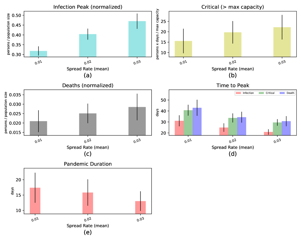
(a) Sensitivity to infection spread rates

(b) Sensitivity to location’s contact rates

Figure 7: Simulator sensitivity to infection spread and contact rates. The plots are generated based on 30 different randomly seeded runs of the simulator. Mean is shown by a solid line and variance either by a shaded region or an error line.

As described in Section 3, we calibrate the simulator to match the historical data that has been observed around the world. While we describe the calibration process in the next section, here we discuss a preliminary analysis of the sensitivity of PandemicSimulator to a few of its important parameters needed for the calibration, namely: (1) spread rates for each person, (2) contact rates for each location, (3) social gatherings size for home parties. Not only this allows us to calibrate PandemicSimulator but it also enables one to establish that the effects of these parameters are roughly as expected. In more detail, we observe how uniformly scaling down or up the default value of these parameters gets reflected in the spread of the pandemic. Then, we use this information to perform a very simple calibration of the simulator against real data.

Figure 7(a), for example, shows that increasing individual spread rates results in increased and faster pandemic peaks. Faster peaks also induce higher numbers of simultaneous critical cases, that easily pass the hospital capacity threshold. Consequently, we observe from our plots that spread rates are directly proportional to number of deaths in PandemicSimulator. Note that this parameter allows us to model super-spreaders on an individual basis. Thus, increasing spread rates practically means increasing the number of super-spreaders and easily infecting most of the simulator’s population.

Figure 8: Simulator sensitivity to social gathering sizes through social events. The plots are generated based on 30 different randomly seeded runs of the simulator. Mean is shown by a solid line and variance either by a shaded region or an error line.

On the contrary, uniformly decreasing contact rates for all locations through a multiplier has the natural effect of reducing the spread of the pandemic, as well as the number of deaths (see Figure 7(b)). This is due to the reduction of contacts among people in the same location, which is also one the implications of social distancing. From our plots, it is possible to observe how the relation between contact rates and number of deaths / critical cases above maximum hospital capacity is non-linear. This non-linearity arises from the limited degrees of separation of our population, which is modeled as a small community where it is easy to be a $2^{\text{nd}}$-degree contact of an infected person when contact rates are not decreased too much.

Social gathering size is another parameter that we analyze in PandemicSimulator. To this end, we compare our metrics with maximum size set at: none (no limit), 5, and 0. As shown in Figure 8, also in this case the relation between the maximum allowed gathering size and deaths / critical cases is non-linear, for the same reasons expressed above. Moreover, the effect of reducing gathering size is even more limited when compared to contact rate results. This is due to the contact rates remaining unchanged, reducing social gatherings to yet another location where the virus can be spread. This suggests that forbidding social gatherings without reducing contact rates or locking other locations might not be productive.

Calibration

For any model to be accepted by real-world decision-makers, they must be provided with a reason to trust that it accurately models the population and spread dynamics in their own community. This trust is typically best instilled via a model calibration process that ensures that the model accurately tracks past data. Based on our parameter sensitivity analysis, we choose to calibrate the simulator by directly controlling the mean of the spread rate distribution, while keeping variance fixed at $0.01$. In fact, while we do not aim at a precise and complex calibration procedure, this is the only parameter among the analyzed ones that has a linear relation to the number of critical cases and deaths, since the parameters of our infection model are already carefully tuned based on previous work reported in Table 2. Specifically, in order to further improve the realism of our model, we compare the average time to peak for deaths and tested critical cases in PandemicSimulator against real data from Sweden, as provided by the World Health Organization. We choose Sweden as our source of data as it represents the nation where the least restrictions have been applied during the first pandemic wave and, thus, where the dynamics of the virus is the most “natural”. In order to match real data (time-to-peak deaths $\approx 30$ days) we run a coarse grained grid search on the spread rate mean in the range $[0.01,0.03]$, resulting in a final parameter choice of $0.03$ (see Figure 7(a)(d), where the simulator’s time-to-peak deaths $\approx 30$ days).

Testing and Contact Tracing

As described in Section 5, to validate PandemicSimulator’s ability to model testing and contact tracing, we compare here several strategies with different testing rates and contact horizons. Specifically, we consider daily testing rates of {0.02, 0.3 (denoted with a + symbol in our plots), and 1.0 (++)} (where 1.0 represents the extreme case of everyone being tested every day) and contact tracing histories of {0, 2, 5, or 10} days. Note that, in our plots, both NONE and SICK use 0 contact tracing history (the second with self-isolation at symptom onset), while CON-$N$ uses an $N$ length history. The full specification of each parameter combination as well as the mapping to the label in Figure 9 is shown in Table 6. For each condition, we ran the experiments with the same 30 random seeds.

Not surprisingly, contact tracing is most beneficial with higher testing rates and longer contact histories because more testing finds more infected people and the contact tracing is able to encourage more of that person’s contacts to stay home. Of course, the best strategy is to test every person every day and quarantine anyone who tests positive (SICK++). Unfortunately, this strategy is impractical except in the most isolated communities. It is interesting to note that this strategy has the highest variance in the time to peak and pandemic duration plots due to the fact that, in this scenario, the virus either stops immediately, or it spreads very slowly.

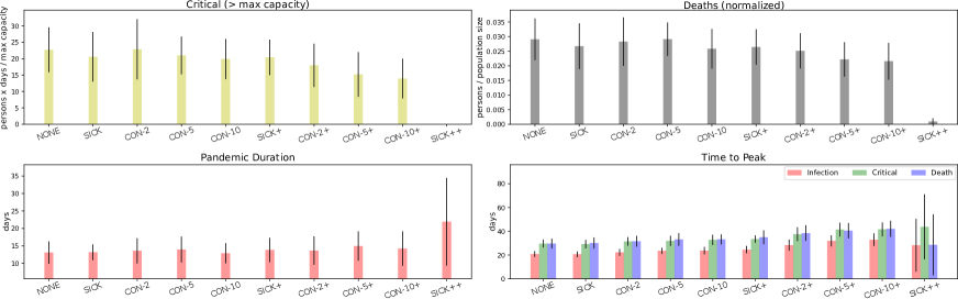
Figure 9: Comparison of various combinations of testing and contact tracing.

Table 6: Testing and contact tracing policies.

Name	Contact tracing history (days)	Random testing rate (daily)	Stay home if sick	Stay home if positive contact
NONE	0	0.02	NO	NO
SICK	0	0.02	YES	NO
CON-2	2	0.02	YES	YES
CON-5	5	0.02	YES	YES
CON-10	10	0.02	YES	YES
SICK+	0	0.3	YES	NO
CON-2+	2	0.3	YES	YES
CON-5+	5	0.3	YES	YES
CON-10+	10	0.3	YES	YES
SICK++	0	1	YES	NO

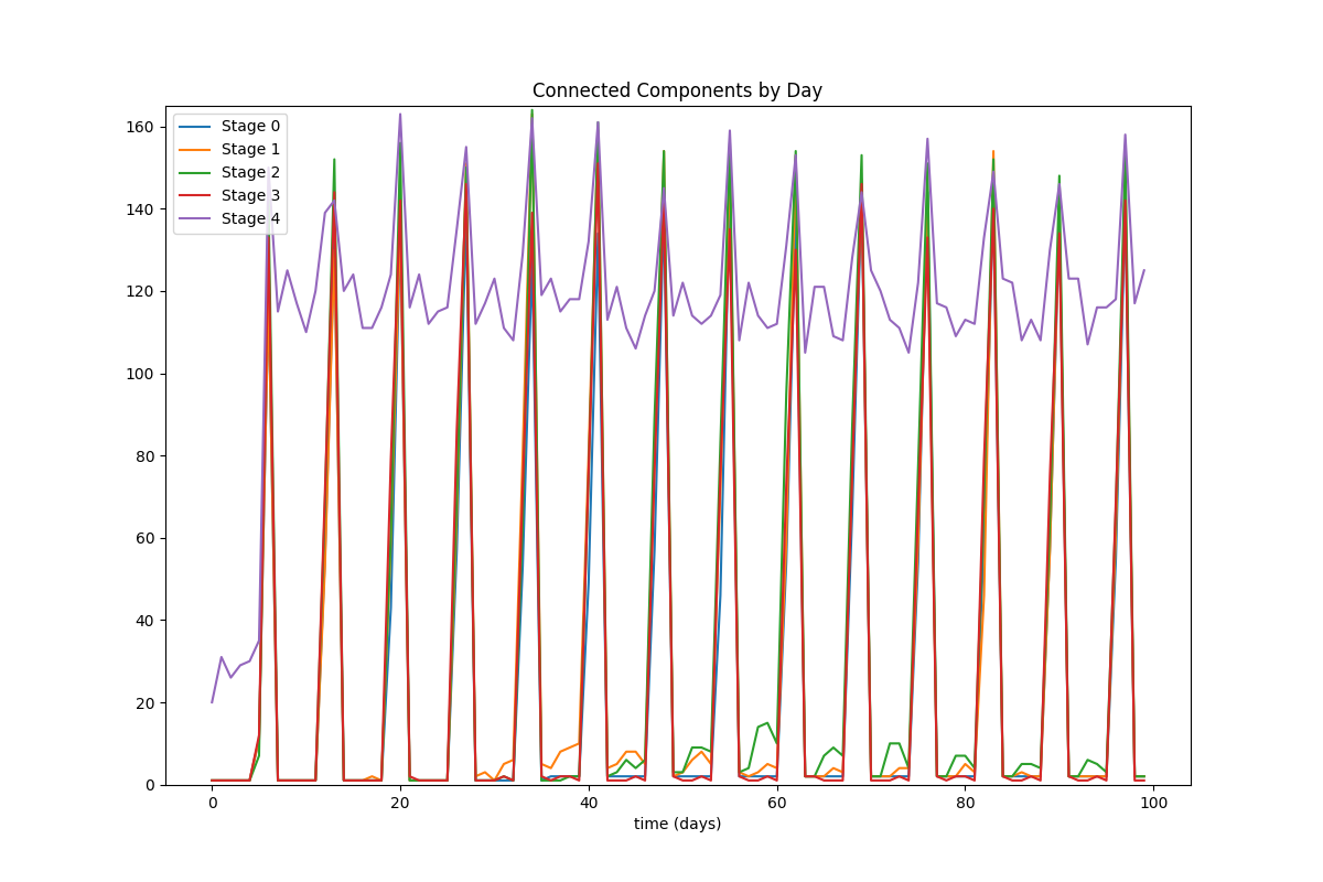
Figure 10: Graph connectivity over 5 different runs, each at a different stage.

Graph Connectivity

One of the ways in which the effects of governmental restrictions can be understood is that they influence the connectivity of the contact graph among members of the population. For example, if the graph is fully connected, the average degree of separation between individuals may be increased by increasing restrictions, which presumably would then slow the spread of the disease.

To investigate the extent to which the restrictions we model influence the graph connectivity, we collected interaction data from runs corresponding to those in Figure 4. From these, we generated a graph of all interactions between the people in the simulator on each day of the simulation.

Our findings indicate that, in fact, the graph is often not connected. We therefore analyze the number of connected components in the interaction graphs during 5 separate runs, each at a different stage. The results are plotted in Figure 10.

As is apparent in the graph, on weekends (the periodic peaks in the graph), the interaction graph has many many separate components, indicating a greater degree of separation between people. Similarly during Stage 4 restrictions, the number of connected components is quite high, suggesting that lockdowns can be very effective in slowing the spread of the pandemic. Somewhat surprisingly, on weekdays at other stages, the number of connected components is relatively low, with relatively small differences between the stages.

An interesting direction for future work is to do a more in-depth graph connectivity analysis, including for interaction graphs that span multiple days.

Simulation Time

In Section 5, we mention that PandemicSimulator can easily handle larger experiments at the cost of greater time and computation. In Table 7, we report simulation times for 1k, 2k, 4k and 10k population environments. For 1k, we also report the training time at which our reinforcement learning algorithm converges.

Table 7: Simulation time for different population sizes. The simulator was run on a single core Intel i7-7700K CPU $@$ 4.2GHz with 32GB of RAM.

Population size	Simulation Time
1k	25.4 msecs/sim-step (our RL training took about 4 hours to converge)
2k	57.9 msecs/sim-step
4k	138.5 msecs/sim-step
10k	500 msecs/sim-step

References

- Aleta et al. (2020) Aleta, A.; Martín-Corral, D.; y Piontti, A. P.; Ajelli, M.; Litvinova, M.; Chinazzi, M.; Dean, N. E.; Halloran, M. E.; Longini Jr, I. M.; Merler, S.; et al. 2020. Modelling the impact of testing, contact tracing and household quarantine on second waves of COVID-19. Nature Human Behaviour 1–8.
- Bansal, Grenfell, and Meyers (2007) Bansal, S.; Grenfell, B. T.; and Meyers, L. A. 2007. When individual behaviour matters: homogeneous and network models in epidemiology. Journal of the Royal Society Interface 4(16): 879–891.
- Brockman et al. (2016) Brockman, G.; Cheung, V.; Pettersson, L.; Schneider, J.; Schulman, J.; Tang, J.; and Zaremba, W. 2016. Openai gym. arXiv preprint arXiv:1606.01540 .
- Cobey (2020) Cobey, S. 2020. Modeling infectious disease dynamics. Science .
- Del Valle, Mniszewski, and Hyman (2013) Del Valle, S. Y.; Mniszewski, S. M.; and Hyman, J. M. 2013. Modeling the impact of behavior changes on the spread of pandemic influenza. In Modeling the interplay between human behavior and the spread of infectious diseases, 59–77. Springer.
- Duque et al. (2020) Duque, D.; Morton, D. P.; Singh, B.; Du, Z.; Pasco, R.; and Meyers, L. A. 2020. COVID-19: How to Relax Social Distancing If You Must. medRxiv doi:10.1101/2020.04.29.20085134. URL https://www.medrxiv.org/content/early/2020/05/05/2020.04.29.20085134.
- Grefenstette et al. (2013) Grefenstette, J. J.; Brown, S. T.; Rosenfeld, R.; DePasse, J.; Stone, N. T.; Cooley, P. C.; Wheaton, W. D.; Fyshe, A.; Galloway, D. D.; Sriram, A.; et al. 2013. FRED (A Framework for Reconstructing Epidemic Dynamics): an open-source software system for modeling infectious diseases and control strategies using census-based populations. BMC public health 13(1): 1–14.
- Gudbjartsson et al. (2020) Gudbjartsson, D. F.; Helgason, A.; Jonsson, H.; Magnusson, O. T.; Melsted, P.; Norddahl, G. L.; Saemundsdottir, J.; Sigurdsson, A.; Sulem, P.; Agustsdottir, A. B.; et al. 2020. Spread of SARS-CoV-2 in the Icelandic population. New England Journal of Medicine .
- Haarnoja et al. (2018) Haarnoja, T.; Zhou, A.; Abbeel, P.; and Levine, S. 2018. Soft Actor-Critic: Off-Policy Maximum Entropy Deep Reinforcement Learning with a Stochastic Actor. In International Conference on Machine Learning, 1861–1870.
- He et al. (2020) He, X.; Lau, E. H.; Wu, P.; Deng, X.; Wang, J.; Hao, X.; Lau, Y. C.; Wong, J. Y.; Guan, Y.; Tan, X.; et al. 2020. Temporal dynamics in viral shedding and transmissibility of COVID-19. Nature medicine 26(5): 672–675.
- Hoertel et al. (2020) Hoertel, N.; Blachier, M.; Blanco, C.; Olfson, M.; Massetti, M.; Sánchez Rico, M.; Limosin, F.; and Leleu, H. 2020. A stochastic agent-based model of the SARS-CoV-2 epidemic in France. Nature Medicine .
- Khadilkar, Ganu, and Seetharam (2020) Khadilkar, H.; Ganu, T.; and Seetharam, D. P. 2020. Optimising Lockdown Policies for Epidemic Control using Reinforcement Learning. Transactions of Indian National Academy of Engineering .
- Larremore et al. (2020) Larremore, D. B.; Wilder, B.; Lester, E.; Shehata, S.; Burke, J. M.; Hay, J. A.; Tambe, M.; Mina, M. J.; and Parker, R. 2020. Test sensitivity is secondary to frequency and turnaround time for COVID-19 surveillance. MedRxiv .
- Libin et al. (2020) Libin, P.; Moonens, A.; Verstraeten, T.; Perez-Sanjines, F.; Hens, N.; Lemey, P.; and Nowé, A. 2020. Deep reinforcement learning for large-scale epidemic control. arXiv preprint arXiv:2003.13676 .
- Liu (2020) Liu, C. 2020. A microscopic epidemic model and pandemic prediction using multi-agent reinforcement learning. arXiv preprint arXiv:2004.12959 .
- Liu et al. (2018) Liu, Q.-H.; Ajelli, M.; Aleta, A.; Merler, S.; Moreno, Y.; and Vespignani, A. 2018. Measurability of the epidemic reproduction number in data-driven contact networks. Proceedings of the National Academy of Sciences 115(50): 12680–12685. ISSN 0027-8424. doi:10.1073/pnas.1811115115. URL https://www.pnas.org/content/115/50/12680.
- Metcalf and Lessler (2017) Metcalf, C. J. E.; and Lessler, J. 2017. Opportunities and challenges in modeling emerging infectious diseases. Science .
- Mnih et al. (2015) Mnih, V.; Kavukcuoglu, K.; Silver, D.; Rusu, A. A.; Veness, J.; Bellemare, M. G.; Graves, A.; Riedmiller, M.; Fidjeland, A. K.; Ostrovski, G.; et al. 2015. Human-level control through deep reinforcement learning. nature 518(7540): 529–533.
- Rivers and Scarpino (2018) Rivers, C. M.; and Scarpino, S. V. 2018. Modelling the trajectory of disease outbreaks works. Nature .
- Song et al. (2020) Song, S.; Zong, Z.; Li, Y.; Liu, X.; and Yu, Y. 2020. Reinforced Epidemic Control: Saving Both Lives and Economy. arXiv preprint arXiv:2008.01257 .
- Sutton and Barto (2018) Sutton, R. S.; and Barto, A. G. 2018. Reinforcement learning: An introduction. MIT press.
- Tindale et al. (2020) Tindale, L.; Coombe, M.; Stockdale, J. E.; Garlock, E.; Lau, W. Y. V.; Saraswat, M.; Lee, Y.-H. B.; Zhang, L.; Chen, D.; Wallinga, J.; et al. 2020. Transmission interval estimates suggest pre-symptomatic spread of COVID-19. MedRxiv .
- Tolles and Luong (2020) Tolles, J.; and Luong, T. 2020. Modeling Epidemics With Compartmental Models. JAMA .
- Verity et al. (2020) Verity, R.; Okell, L. C.; Dorigatti, I.; Winskill, P.; Whittaker, C.; Imai, N.; Cuomo-Dannenburg, G.; Thompson, H.; Walker, P. G.; Fu, H.; et al. 2020. Estimates of the severity of coronavirus disease 2019: a model-based analysis. The Lancet infectious diseases .
- Xiao et al. (2020) Xiao, Y.; Yang, M.; Zhu, Z.; Yang, H.; Zhang, L.; and Ghader, S. 2020. Modeling indoor-level non-pharmaceutical interventions during the COVID-19 pandemic: a pedestrian dynamics-based microscopic simulation approach. arXiv preprint arXiv:2006.10666 .
- Zhang et al. (2020) Zhang, J.; Litvinova, M.; Wang, W.; Wang, Y.; Deng, X.; Chen, X.; Li, M.; Zheng, W.; Yi, L.; Chen, X.; et al. 2020. Evolving epidemiology and transmission dynamics of coronavirus disease 2019 outside Hubei province, China: a descriptive and modelling study. The Lancet Infectious Diseases .