Precise predictions for photon pair production matched to parton showers in GENEVA

Abstract

We present a new calculation for the production of isolated photon pairs at the LHC with NNLL${}^{\prime}_{\mathcal{T}_{0}}$+NNLO accuracy. This is the first implementation within the Geneva Monte Carlo framework of a process with a nontrivial Born-level definition which suffers from QED singularities. Throughout the computation we use a smooth-cone isolation algorithm to remove such divergences. The higher-order resummation of the $0$-jettiness resolution variable $\mathcal{T}_{0}$ is based on a factorisation formula derived within Soft-Collinear Effective Theory which predicts all of the singular, virtual and real NNLO corrections. Starting from this precise parton-level prediction and by employing the Geneva method, we provide fully showered and hadronised events using Pythia8, while retaining the NNLO QCD accuracy for observables which are inclusive over the additional radiation. We compare our final predictions to LHC data at 7 TeV and find good agreement.

1 Introduction

The production of two isolated photons is one of the most interesting processes to study at the Large Hadron Collider (LHC), both to further test the Standard Model (SM) and to search for new exotic signatures, e.g. by looking for heavy resonances in the diphoton invariant mass spectrum TheATLAScollaboration:2015mdt ; CMS:2015dxe . Precise experimental measurements are available due to the clean final state and the relatively high rate of production for this process. Efforts in the study of the diphoton final state were especially boosted by the discovery of a Higgs boson decaying into two photons at the LHC Aad:2012tfa ; Chatrchyan:2012ufa . For all these reasons, recent experimental analyses of diphoton production have been carried out by the ATLAS experiment both at 7 TeV Aad:2011mh ; Aad:2012tba , 8 TeV Aaboud:2017vol and 13 TeV ATLAS:2020qqv , and by CMS at 7 TeV Chatrchyan:2011qt ; Chatrchyan:2014fsa . Given the relevance of this process for the LHC experimental analyses, precise calculations including higher-order QCD corrections are required from the theoretical side.

In this paper we study the production of “prompt” photon pairs which are directly produced in the hard scattering interaction. A second production mechanism involves the radiation of photons in a jet during the fragmentation process. This second mechanism can be suppressed by isolating the photons from the final-state hadrons with either the fixed-cone or the smooth-cone (a.k.a. Frixione) isolation procedure Frixione:1998jh . The fixed-cone isolation is widely used in the experimental analyses due to the simplicity of its implementation. It cannot, however, completely eliminate the fragmentation contribution without spoiling infrared (IR) safety. The smooth-cone isolation can achieve this in an IR-safe manner, thus simplifying the computation of the radiative corrections.

Next-to-leading-order (NLO) QCD corrections for the process $pp/p\bar{p}\to\gamma\gamma+X$ were first computed and implemented in the fully differential Monte Carlo program DIPHOX Binoth:1999qq which included the calculation of both the “direct” and the fragmentation contributions to the cross section. The leading-order (LO) calculation Dicus:1987fk of the gluon channel $gg\to\gamma\gamma$ contribution, which is formally a next-to-next-to-leading-order (NNLO) effect, was also implemented in the DIPHOX code. The inclusion of this channel has a relatively large impact on the cross section, due to the enhanced gluon parton distributions at the LHC. The NLO corrections to the gluon channel (which amount to N³LO effects relative to the LO process $q\bar{q}\to\gamma\gamma$) were implemented in the parton-level Monte Carlo programs 2gammaMC Bern:2002jx and MCFM Campbell:2011bn . Recently, mass effects due to the top-quark loops were studied in the gluon fusion channel at NLO accuracy in Refs. Maltoni:2018zvp ; Chen:2019fla .

In the context of smooth-cone isolation, where fragmentation functions are not required, the first NNLO calculation for diphoton production was carried out at the fully differential level using the $q_{T}$ subtraction method of Ref. Catani:2007vq . It has been implemented in the numerical codes 2$\gamma$NNLO Catani:2011qz and Matrix Grazzini:2017mhc . An independent calculation at NNLO accuracy for diphoton production was also performed in Ref. Campbell:2016yrh and implemented in the MCFM program Boughezal:2016wmq . This calculation uses the $N$-jettiness subtraction method Boughezal:2015dva ; Gaunt:2015pea derived within Soft-Collinear Effective Theory (SCET). Phenomenological studies of photon isolation at NNLO accuracy were carried out in Ref. Catani:2018krb by using the aforementioned programs 2$\gamma$NNLO and Matrix. More recently, an independent NNLO analysis using the antenna subtraction method GehrmannDeRidder:2005cm ; Daleo:2006xa ; Currie:2013vh was presented in Ref. Gehrmann:2020oec , highlighting the importance of the choice of the isolation criterion and of the scales in estimating the theoretical uncertainties. Electroweak (EW) corrections for the diphoton production process at the LHC were computed in Refs. Bierweiler:2013dja ; Chiesa:2017gqx . Their effect for inclusive observables is at the level of a few percent, and increases as one imposes higher transverse-momentum cuts on the photons.

Resummed calculations in the region of small transverse momentum of the photon pair have been carried out at next-to-next-to-leading logarithmic (NNLL) accuracy and are available in the programs RESBOS Balazs:2006cc ; Nadolsky:2007ba ; Balazs:2007hr , 2$\gamma$Res Cieri:2015rqa and reSolve Coradeschi:2017zzw . Very recently, the resummation was pushed to N³LL accuracy in CuTe-MCFM Becher:2020ugp , extending the matching to NNLO accuracy. The process is also available at this accuracy in the public interface MATRIX+RadISH Kallweit:2020gva .

Shower Monte Carlo (SMC) simulations for this process at NLO accuracy matched to the Sherpa Gleisberg:2008ta parton shower program were presented in Ref. Hoeche:2009xc . A similar accuracy obtained via matching to the Herwig Corcella:2000bw parton shower using the Powheg approach Nason:2004rx ; Frixione:2007vw was presented in Ref. DErrico:2011cgc .

In this paper we implement a new fully differential NNLO event generator for the diphoton production process $pp\to\gamma\gamma+X$. We improve on the existing fixed-order (FO) calculations by including the NNLL${}^{\prime}_{\mathcal{T}_{0}}$ resummation of the $0$-jettiness resolution variable $\mathcal{T}_{0}$ (beam thrust) within the Geneva Monte Carlo framework Alioli:2012fc ; Alioli:2013hqa ; Alioli:2015toa ; Alioli:2016wqt . The resummation of the $0$-jettiness variable is carried out by using a factorisation formula Stewart:2009yx ; Stewart:2010pd valid at small $\mathcal{T}_{0}$ derived in SCET. This is the first time that such a resummation has been presented in the literature for this process. We employ the smooth-cone isolation algorithm to define IR-finite events, ensuring that the application of this cut is compatible with the $\mathcal{T}_{0}$ resummation. In addition, we provide fully showered and hadronised events by matching partonic events to the Pythia8 Sjostrand:2014zea parton shower while retaining the FO accuracy for inclusive observables. Diphoton production extends the list of NNLO+PS processes, such as Drell–Yan Alioli:2015toa and associated Higgs production Alioli:2019qzz and decay Alioli:2020fzf , which were previously implemented in the Geneva Monte Carlo program. Alternative approaches to reach NNLO+PS accuracy are actively being developed Hamilton:2012rf ; Hamilton:2013fea ; Monni:2019whf ; Monni:2020nks ; Hoeche:2014aia ; Hoche:2014dla .

This paper is organised as follows. We discuss the process definition and the photon isolation criteria in sec. 2. In sec. 3 we recap the theoretical background for the $0$-jettiness resummation in SCET, while in sec. 4 we provide the details of the implementation in the Geneva framework. We present our results in sec. 5, including the comparison to 7 TeV LHC data. Finally we give our conclusions and outlook in sec. 6.

2 Process definition and photon isolation

In this paper we consider the process

$$p\,p\to\gamma\,\gamma+X\,,$$

where the photon pair is produced through the hard scattering interaction (i.e. direct photon production). In order to avoid QED singularities when a photon is collinear to an initial-state parton, one needs to impose kinematic cuts on the transverse momenta of the photons. We prefer to use asymmetric cuts on the harder ($\gamma_{h}$) and the softer ($\gamma_{s}$) photon, i.e. $p^{\gamma_{h}}_{T}\geq p^{\gamma_{h}}_{T,\textrm{cut}}$ and $p^{\gamma_{s}}_{T}\geq p^{\gamma_{s}}_{T,\textrm{cut}}$ (where $p^{\gamma_{h}}_{T}\geq p^{\gamma_{s}}_{T}$) which avoids issues in the fixed-order predictions with symmetric cuts Frixione:1997ks ; Banfi:2003jj ; Alioli:2012tp . These cuts are also employed in experimental analyses to exclude events in which the photons are emitted in the uninstrumented region parallel to the beam line.

As mentioned in the introduction, final-state photons can also be produced via the fragmentation of a quark or a gluon into a photon. Usually, photons produced in a fragmentation process are distinguishable from the direct photons since they lie inside hadronic jets. Direct photons can therefore be separated from the rest of the hadrons in the event through an isolation procedure. A possible isolation mechanism is to construct a cone with fixed radius $R_{\textrm{iso}}$ around the direction of the photon candidate. One then restricts the amount of transverse hadronic (partonic) energy $E^{\textrm{had}}_{T}(R_{\textrm{iso}})$ inside the cone. In particular, a photon is considered to be isolated if $E^{\textrm{had}}_{T}(R_{\textrm{iso}})$ is smaller than a certain value $E^{\textrm{max}}_{T}$, usually parameterised as a (linear) function of the transverse energy $E^{\gamma}_{T}$ of the photon and a fixed numerical value $E^{\textrm{thres}}_{T}$ Catani:2002ny :

$$E^{\textrm{had}}_{T}(R_{\textrm{iso}})<E^{\textrm{max}}_{T}\equiv\varepsilon\,E^{\gamma}_{T}+E^{\textrm{thres}}_{T}\,.$$ (1)

Due to its simplicity, the fixed-cone isolation procedure is currently used in all experimental measurements of processes involving photons. This method has the theoretical drawback of being sensitive to the fragmentation contributions since configurations with a photon collinear to a final-state parton are still allowed. Indeed, to completely remove the collinear QED divergences, one should require that absolutely no hadronic energy is allowed within the cone. Unfortunately, this condition is not IR safe since it forbids emissions of soft partons inside the cone, therefore spoiling the cancellation of QCD divergences.

The smooth-cone isolation procedure instead overcomes this problem by considering a continuous series of smaller sub-cones with radius $r\leq R_{\textrm{iso}}$, in addition to the outer cone of radius $R_{\textrm{iso}}$. The isolation condition then requires that

$$E^{\textrm{had}}_{T}(r)\leq E^{\textrm{max}}_{T}\,\chi(r;R_{\textrm{iso}})\,,\quad\textrm{for all sub-cones with}\,\,r\leq R_{\textrm{iso}}\,,$$ (2)

where the isolation function $\chi(r;R_{\textrm{iso}})$ must be a smooth and monotonic function which vanishes when $r\to 0$. This requirement implies that the hadronic activity is reduced in a smooth way when approaching the photon direction, and the parton radiation collinear to the photon is completely absent at $r=0$. Hence, the fragmentation component is eliminated while soft radiation is still permitted in a finite region away from the collinear limit, making the cross section IR safe. The standard choice for the $\chi$-function is

$$\chi(r;R_{\text{iso}})=\left(\frac{1-\cos r}{1-\cos{R_{\text{iso}}}}\right)^{n}\!,$$ (3)

where the exponent parameter $n$ is usually set to $n=1$. Other isolation functions satisfying these criteria are possible and have been employed in the literature Catani:2018krb .

Though the use of a smooth-cone isolation procedure has the positive effect of simplifying theoretical calculations, its implementation in the experimental analyses is complicated by the granular nature of the detector. The direct comparison of the theoretical predictions with data is therefore challenging. One possible solution is to adjust the free parameters of the smooth-cone isolation algorithm to reproduce the effects of the fixed-cone procedure, making a comparison at least feasible. A potentially better approach, which has been recently investigated in Refs. Siegert:2016bre ; Chen:2019zmr , is the introduction of a hybrid-cone isolation procedure. In this case the theoretical calculation is initially carried out using the smooth-cone isolation with a very small radius parameter $R_{\text{iso}}$, such that only a tiny slice of phase space around the photon direction is removed. In a second step, the fixed-cone isolation procedure with a larger radius $R\gg R_{\text{iso}}$ is applied to the events which passed the smooth-cone criterion. In other words, one initially applies very loose smooth-cone isolation cuts which are then tightened by the fixed-cone procedure. This makes the resulting events directly suitable for experimental analyses. In this paper we investigate both the smooth-cone and the hybrid-cone isolation procedures. We use the former to compare to results obtained with the Matrix code Grazzini:2017mhc in sec. 4.5, while the latter is used for a direct comparison to LHC data in sec. 5.

3 Resummation in Soft-Collinear Effective Theory

In this work, we use the $N$-jettiness Stewart:2010tn resolution variable to discriminate between resolved emissions with different jet multiplicities. Given an $M$-particle phase space point $\Phi_{M}$ with $M\geq N$, the $N$-jettiness is defined as

$$\mathcal{T}_{N}(\Phi_{M})=\sum_{k}\textrm{min}\big{\{}\hat{q}_{a}\cdot p_{k},\hat{q}_{b}\cdot p_{k},\hat{q}_{1}\cdot p_{k},\ldots,\hat{q}_{N}\cdot p_{k}\big{\}}\,,$$ (4)

where the index $k$ runs over all strongly-interacting final-state particles and where $\hat{q}_{i}=n_{i}=(1,\vec{n}_{i})$ are light-like reference vectors parallel to the beam and jet directions, defined in the rest frame of the $\gamma\gamma$ colour-singlet state. The limit $\mathcal{T}_{N}\to 0$ describes an event with $N$ pencil-like hard jets, where the unresolved emissions can either be soft or collinear to the final-state jets or to the beams. In the case of colour-singlet production (e.g. Drell–Yan, $VH$, $\gamma\gamma$, …) the relevant resolution variable is the $0$-jettiness (beam thrust). Starting from the general definition in eq. (4), the expression for the $0$-jettiness can be considerably simplified to

$$\mathcal{T}_{0}=\sum_{k}|\vec{p}_{kT}|\,e^{-|\eta_{k}-Y|}\,,$$ (5)

where $|\vec{p}_{kT}|$ and $\eta_{k}$ are the transverse momentum and the rapidity of the emission $p_{k}$ and $Y$ is the rapidity of the colour-singlet state.

The introduction of a jet resolution variable sets a new dynamical energy scale in the problem, which can in principle differ from the other physical scales of the process. As such, large logarithms of the ratios of these scales may appear in the cross section which spoil the convergence of the perturbative expansion and must therefore be resummed. For $0$-jettiness this happens in the small $\mathcal{T}_{0}/Q$ region, with $Q$ being a typical hard scale of the process, e.g. the invariant mass of the colour-singlet final state. In this region, the cross section differential in the Born phase space $\Phi_{0}$ and $\mathcal{T}_{0}$ obeys a factorisation formula which was originally derived in Refs. Stewart:2009yx ; Stewart:2010pd for the Drell–Yan process, but which can be extended for diphoton production as

$$\frac{\textrm{d}\sigma^{\text{SCET}}}{\textrm{d}\Phi_{0}\textrm{d}\mathcal{T}_{0}}=\Theta^{\mathrm{PS}}(\Phi_{0})\sum_{ij}H^{\gamma\gamma}_{ij}(Q^{2},t,\mu)\int\!\mathrm{d}r_{a}\,\mathrm{d}r_{b}\, B_{i}(r_{a},x_{a},\mu)B_{j}(r_{b},x_{b},\mu)\,S(\mathcal{T}_{0}-\tfrac{r_{a}+r_{b}}{Q},\mu)\,.$$ (6)

The sum in the equation above runs over all possible $q\bar{q}$ pairs $ij=\{u\bar{u},\bar{u}u,d\bar{d},\bar{d}d,\ldots\}$. For this process we need to impose process-defining phase space restrictions $\Theta^{\mathrm{PS}}(\Phi_{0})$ in order to have a finite cross section. In particular, we apply $p_{T}$ cuts on each of the photons as well as isolation cuts to eliminate final-state collinear QED singularities. Other cuts, such as on the photons’ rapidities or on the invariant mass of the pair, can be imposed at the analysis level but are not needed to define IR-finite cross sections.

The factorisation formula depends on the hard $H^{\gamma\gamma}_{ij}$, soft $S$ and beam $B_{i,j}$ functions which describe the square of the hard interaction Wilson coefficients, the soft real emissions between external partons and the hard emissions collinear to the beams respectively.

The hard functions $H^{\gamma\gamma}_{ij}(Q^{2},t,\mu)$ are process-dependent objects and encode information about the Born and virtual squared matrix elements. In order to achieve NNLL^′ accuracy, they are needed up to two-loop order. They are regular functions of the Mandelstam invariants $Q^{2}=s$ and $t$ and can be extracted from the two-loop squared amplitude expressions Anastasiou:2002zn , after subtracting the IR poles (as explained in detail in appendix A).

The $B_{i}(r,x,\mu)$ are the inclusive (anti-)quark beam functions Stewart:2009yx . They depend on the virtualities $r_{a,b}$ of the initial-state partons $i$ and $j$ annihilated in the hard interaction and on the momentum fractions $x_{a,b}$. These can be written in terms of the diphoton rapidity $Y_{\gamma\gamma}$ and invariant mass $M_{\gamma\gamma}$ as

$$x_{a}=\frac{M_{\gamma\gamma}}{E_{\textrm{cm}}}e^{Y_{\gamma\gamma}},\quad x_{b}=\frac{M_{\gamma\gamma}}{E_{\textrm{cm}}}e^{-Y_{\gamma\gamma}}\,,$$ (7)

where $E_{\textrm{cm}}$ is the hadronic centre-of-mass energy. The beam functions are calculated via an operator product expansion and are defined as

$$B_{i}(r_{a},x_{a},\mu)=\sum_{k}\int_{x_{a}}^{1}\frac{\mathrm{d}\xi_{a}}{\xi_{a}}\,\mathcal{I}_{ik}\bigg{(}r_{a},\frac{x_{a}}{\xi_{a}},\mu\bigg{)}\,f_{k}(\xi_{a},\mu)\,.$$ (8)

The perturbatively computable parts of the above equation are the matching coefficients $\mathcal{I}_{ik}(t_{a},z_{a},\mu)$ which describe the collinear virtual and real initial-state radiation (ISR) emissions. The function $f_{k}(\xi_{a},\mu)$ represents the usual parton distribution function (PDF) for parton $k$ with momentum fraction $\xi_{a}$. The matching coefficients $\mathcal{I}_{ik}(t_{a},z_{a},\mu)$ were computed to NNLO accuracy in Ref. Gaunt:2014xga . $S(k,\mu)$ is the quark hemisphere soft function for beam thrust and has been computed to the required NNLO accuracy including the scale independent terms in Refs. Kelley:2011ng ; Monni:2011gb .

The hard, beam and soft functions which appear in eq. (6) are single-scale objects. This means that when they are evaluated at their own characteristic scales

$$\mu_{H}=Q,\quad\mu_{B}=\sqrt{Q\mathcal{T}_{0}},\quad\mu_{S}=\mathcal{T}_{0}\,,$$ (9)

no large logarithmic corrections are present in their fixed-order perturbative expansions. However, eq. (6) must be evaluated at a single common scale $\mu$. In order to do this, the separate components must be evolved via renormalisation group (RG) equations from their own characteristic scales to the common scale $\mu$, which results in the large logarithms being resummed. This proceeds via convolutions of the single scale factors with the evolution functions $U_{i}(\mu_{i},\mu)$. The resummed formula for the $\mathcal{T}_{0}$ spectrum is then given by

$$\frac{\textrm{d}\sigma^{\text{NNLL}^{\prime}}}{\textrm{d}\Phi_{0}\textrm{d}\mathcal{T}_{0}}=\; \Theta^{\mathrm{PS}}(\Phi_{0})\sum_{ij}H^{\gamma\gamma}_{ij}(Q^{2},t,\mu_{H})\,U_{H}(\mu_{H},\mu)\,\big{\{}\big{[}B_{i}(t_{a},x_{a},\mu_{B})\otimes U_{B}(\mu_{B},\mu)\big{]}\,$$

$$\times\big{[}B_{j}(t_{b},x_{b},\mu_{B})\otimes U_{B}(\mu_{B},\mu)\big{]}\big{\}}\,\otimes\big{[}S(\mu_{s})\otimes U_{S}(\mu_{S},\mu)\big{]}\,,$$ (10)

where the convolution between the different functions is written in a schematic form. The scale setting procedure will be explained in the next section, where we will introduce the profile functions which are employed to switch off resummation outside its kinematical range of validity. In order to reach NNLL^′ accuracy, we need to know the boundary conditions of the evolution, namely the hard, beam and soft functions up to NNLO accuracy, and the cusp (non-cusp) anomalous dimensions up to three-(two-)loop order. The expressions for the anomalous dimensions up to the required order can be found in Refs. Idilbi:2006dg ; Becher:2006mr ; Hornig:2011iu ; Kang:2015moa ; Gaunt:2015pea .

4 Implementation within the GENEVA framework

In this section we review the Geneva framework and present the implementation of the diphoton production process, highlighting the main differences compared to the processes that have previously been implemented. More details on the general features of the Geneva method are given in Refs. Alioli:2013hqa ; Alioli:2015toa ; Alioli:2019qzz .

For all numerical results in this paper we evaluate all the matrix elements up to the one-loop level with the amplitudes provided by the OpenLoops 2 package Cascioli:2011va ; Buccioni:2017yxi ; Buccioni:2019sur . We include the top-quark mass dependence in the NLO calculation of the diphoton plus jet production process and set $m_{t}=173.2$ GeV. In the present implementation, however, we do not include the diagrams with a closed top-quark loop in the hard function. These effects begin to contribute at $\mathcal{O}(\alpha_{s}^{2})$ and are currently unknown in the $q\bar{q}$ channel.

If not stated otherwise, in this section we use the following settings: we use the MMHT2014nnlo68cl PDF set Harland-Lang:2014zoa from LHAPDF Buckley:2014ana and the $\alpha(0)$ input scheme to fix EW couplings and set $\alpha^{-1}(0)=137$. We apply the kinematic cuts

$$p^{\gamma_{h}}_{T}\geq 25\,\,\mathrm{GeV},\quad p^{\gamma_{s}}_{T}\geq 22\,\,\mathrm{GeV},\quad M_{\gamma\gamma}\geq 25\,\,\mathrm{GeV}\,,$$ (11)

and the smooth-cone isolation algorithm with parameters

$$E^{\mathrm{max}}_{T}=4\,\,\mathrm{GeV},\quad R_{\mathrm{iso}}=0.4,\quad\mathrm{and}\quad n=1\,.$$ (12)

We set $\mu_{\mathrm{FO}}=M_{\gamma\gamma}$ or $\mu_{\mathrm{FO}}=M_{\gamma\gamma}^{T}\equiv\sqrt{M^{2}_{\gamma\gamma}+p^{2}_{T,\gamma\gamma}}$ and indicate the respective choice with the results. We consider only the $q\bar{q}$ channel contribution up to and including sec. 4.7 and take into account also the loop-induced $gg$ channel contribution thereafter.

4.1 The GENEVA method

The final aim of a fully exclusive event generator is to produce physical events, where all of the IR divergences are cancelled on an event-by-event basis. Following the Geneva method, these events are assigned a Monte Carlo (MC) cross section $\mathrm{d}\sigma^{\mathrm{MC}}_{N}$ according to the value of the $N$-jettiness resolution parameter $\mathcal{T}_{N}$. This encodes the probability of producing a phase space point $\Phi_{N}$ with $N$ partonic jets: all contributions from unresolved emissions below a certain resolution cutoff $\mathcal{T}_{N}<\mathcal{T}^{\text{cut}}_{N}$ are included in $\mathrm{d}\sigma^{\mathrm{MC}}_{N}$. For the process at hand at NNLO, the exclusive cross sections for events with $0$ and $1$ jet, and the $2$-jet inclusive cross section are defined by the cutoffs on the $\mathcal{T}_{0}$ and $\mathcal{T}_{1}$ resolution variables as

$$\Phi_{0} \qquad\frac{\mathrm{d}\sigma^{\textsc{mc}}_{0}}{\mathrm{d}\Phi_{0}}(\mathcal{T}_{0}^{\mathrm{cut}})\,,$$ events:

$$\Phi_{1} \qquad\frac{\mathrm{d}\sigma^{\textsc{mc}}_{1}}{\mathrm{d}\Phi_{1}}(\mathcal{T}_{0}>\mathcal{T}_{0}^{\mathrm{cut}};\mathcal{T}_{1}^{\mathrm{cut}})\,,$$ events:

$$\Phi_{2} \qquad\frac{\mathrm{d}\sigma^{\textsc{mc}}_{\geq 2}}{\mathrm{d}\Phi_{2}}(\mathcal{T}_{0}>\mathcal{T}_{0}^{\mathrm{cut}},\mathcal{T}_{1}>\mathcal{T}_{1}^{\mathrm{cut}})\,.$$ events: (13)

Since one integrates over the unresolved emissions below the cutoffs, the definitions of the partonic jets used above depend on the phase space maps $\Phi_{N}(\Phi_{M})$ (with $N\leq M$) which project the unresolved $M$-body phase space points onto $\Phi_{N}$. Using eq. (4.1) the cross section for a generic observable $X$ is written as

$$\sigma(X) =\int\!\mathrm{d}\Phi_{0}\,\frac{\mathrm{d}\sigma^{\textsc{mc}}_{0}}{\mathrm{d}\Phi_{0}}(\mathcal{T}_{0}^{\mathrm{cut}})\,M_{X}(\Phi_{0})$$

$$\quad+\int\!\mathrm{d}\Phi_{1}\,\frac{\mathrm{d}\sigma^{\textsc{mc}}_{1}}{\mathrm{d}\Phi_{1}}(\mathcal{T}_{0}>\mathcal{T}_{0}^{\mathrm{cut}};\mathcal{T}_{1}^{\mathrm{cut}})\,M_{X}(\Phi_{1})$$

$$\quad+\int\!\mathrm{d}\Phi_{2}\,\frac{\mathrm{d}\sigma^{\textsc{mc}}_{\geq 2}}{\mathrm{d}\Phi_{2}}(\mathcal{T}_{0}>\mathcal{T}_{0}^{\mathrm{cut}},\mathcal{T}_{1}>\mathcal{T}_{1}^{\mathrm{cut}})\,M_{X}(\Phi_{2})\,,$$ (14)

where $M_{X}(\Phi_{N})$ is the measurement function that computes the observable $X$ for the $N$-parton final-state point $\Phi_{N}$.

The cross section defined above is not equivalent to that obtained from a fixed-order calculation. Indeed, for any unresolved emission, the observable is computed on the projected point $\Phi_{N}(\Phi_{M})$ rather than the exact $\Phi_{M}$ point. Since the resulting difference vanishes in the limit $\mathcal{T}^{\textrm{cut}}_{N}\to 0$, it is advisable to choose this cutoff to be as small as possible. This, however, introduces large logarithms of $\mathcal{T}_{N}$ and $\mathcal{T}^{\textrm{cut}}_{N}$, which need to be resummed in order to obtain physically meaningful results.

We perform the resummation of $\mathcal{T}_{0}$ at NNLL^′ accuracy, matching it to a NNLO₀ calculation. This has the positive feature of correctly describing the spectrum both in the small-$\mathcal{T}_{0}$ region, where the resummation dominates, and also in the large-$\mathcal{T}_{0}$ region, where the correct dependence is given by the fixed-order result.

Depending on the final-state jet multiplicity, the Geneva method requires one to evaluate the resummed and resummed-expanded terms in the cross sections on projected phase space points of lower multiplicity. Even these projected configurations are required to satisfy the cuts which avoid the QED singularities. We use the symbol $\Theta^{\mathrm{proj}}(\widetilde{\Phi}_{N})$ (and $\overline{\Theta}^{\mathrm{proj}}(\widetilde{\Phi}_{N})$ for its complement) to indicate this set of phase space restrictions acting on the higher dimensional $\Phi_{N+1}$ phase space due to the cuts on the projected configuration $\widetilde{\Phi}_{N}$. In practice, this means that when a term in the cross section, evaluated at a $\Phi_{N+1}$ phase space point, is multiplied by $\Theta^{\mathrm{proj}}(\widetilde{\Phi}_{N})$, the $\Phi_{N+1}$ phase space point is projected onto a $\widetilde{\Phi}_{N}$ point and the cuts are applied on this lower dimensional space. If the projected configuration does not pass the cuts, the initial $\Phi_{N+1}$ configuration is excluded. Notice that the separation realised by the introduction of $\Theta^{\mathrm{proj}}$ and $\overline{\Theta}^{\mathrm{proj}}$ is not usually required in a fixed-order calculation. Nonetheless, we choose to perform it even when evaluating the FO contribution and split this into two parts. Of these, the first, singular part enters in the $0$-jet cumulant, eq. (4.1), while the second, nonsingular part enters in the $1$-jet cross section below the $\mathcal{T}_{0}^{\rm cut}$, eq. (24).

Since the resummation for $0$-jettiness is carried out at NNLL^′ accuracy in Geneva, meaning that it contains all of the singular corrections in $\mathcal{T}_{0}$ up to $\mathcal{O}(\alpha^{2}_{s})$, we can write the 0- and 1-jet cross sections as

$$\frac{\mathrm{d}\sigma^{\textsc{mc}}_{0}}{\mathrm{d}\Phi_{0}}(\mathcal{T}_{0}^{\mathrm{cut}})= \;\frac{\mathrm{d}\sigma^{\rm NNLL^{\prime}}}{\mathrm{d}\Phi_{0}}(\mathcal{T}_{0}^{\mathrm{cut}})+\frac{\mathrm{d}\sigma_{0}^{\rm nons}}{\mathrm{d}\Phi_{0}}(\mathcal{T}_{0}^{\mathrm{cut}})\,,$$ (15)

$$\frac{\mathrm{d}\sigma^{\textsc{mc}}_{\geq 1}}{\mathrm{d}\Phi_{1}}(\mathcal{T}_{0}>\mathcal{T}_{0}^{\mathrm{cut}})= \left[\!\frac{\mathrm{d}\sigma^{\rm NNLL^{\prime}}}{\mathrm{d}\Phi_{0}\mathrm{d}\mathcal{T}_{0}}\,\mathcal{P}(\Phi_{1})\,\Theta^{\mathrm{PS}}(\Phi_{1})\Theta^{\mathrm{proj}}(\widetilde{\Phi}_{0})\!+\!\frac{\mathrm{d}\sigma_{\geq 1}^{\rm nons}}{\mathrm{d}\Phi_{1}}(\mathcal{T}_{0}>\mathcal{T}_{0}^{\mathrm{cut}})\!\right]\!\theta(\mathcal{T}_{0}>\mathcal{T}_{0}^{\mathrm{cut}}),$$ (16)

where $\mathrm{d}\sigma^{\rm NNLL^{\prime}}/\mathrm{d}\Phi_{0}\mathrm{d}\mathcal{T}_{0}$ is the resummed $\mathcal{T}_{0}$ spectrum and $\mathrm{d}\sigma^{\rm NNLL^{\prime}}/\mathrm{d}\Phi_{0}(\mathcal{T}_{0}^{\mathrm{cut}})$ is its integral. In the above equation we introduced a splitting probability function $\mathcal{P}(\Phi_{1})$ which satisfies the normalisation condition

$$\int\!\frac{\mathrm{d}\Phi_{1}}{\mathrm{d}\Phi_{0}\mathrm{d}\mathcal{T}_{0}}\,\mathcal{P}(\Phi_{1})=1$$ (17)

to make the $\mathcal{T}_{0}$ spectrum fully differential in $\Phi_{1}$. The nonsingular contributions are given by

$$\frac{\mathrm{d}\sigma_{0}^{\mathrm{nons}}}{\mathrm{d}\Phi_{0}}(\mathcal{T}_{0}^{\mathrm{cut}})= \;\frac{\mathrm{d}\sigma_{0}^{{\rm NNLO_{0}}}}{\mathrm{d}\Phi_{0}}(\mathcal{T}_{0}^{\mathrm{cut}})-\biggl{[}\frac{\mathrm{d}\sigma^{\rm NNLL^{\prime}}}{\mathrm{d}\Phi_{0}}(\mathcal{T}_{0}^{\mathrm{cut}})\biggr{]}_{\rm NNLO_{0}}\,,$$ (18)

$$\frac{\mathrm{d}\sigma_{\geq 1}^{\mathrm{nons}}}{\mathrm{d}\Phi_{1}}(\mathcal{T}_{0}>\mathcal{T}_{0}^{\mathrm{cut}})= \;\frac{\mathrm{d}\sigma_{\geq 1}^{{\rm NLO_{1}}}}{\mathrm{d}\Phi_{1}}(\mathcal{T}_{0}>\mathcal{T}_{0}^{\mathrm{cut}})-\biggl{[}\frac{\mathrm{d}\sigma^{\rm NNLL^{\prime}}}{\mathrm{d}\Phi_{0}\mathrm{d}\mathcal{T}_{0}}\mathcal{P}(\Phi_{1})\biggr{]}_{\rm NLO_{1}}\!\!\!\Theta^{\mathrm{PS}}(\Phi_{1})\,\Theta^{\mathrm{proj}}(\widetilde{\Phi}_{0})\,.$$ (19)

The terms in squared brackets are the expanded expressions to $\mathcal{O}(\alpha^{2}_{s})$ of the resummed cumulant and spectrum. The NLO₁ term refers to the NLO corrections to the diphoton plus jet production process. The projected $\Phi_{1}\to\widetilde{\Phi}_{0}$ point in the above equation is obtained through a FKS projection. After explicitly writing the FO contributions to the cross sections we obtain

$$\frac{\mathrm{d}\sigma^{\textsc{mc}}_{0}}{\mathrm{d}\Phi_{0}}(\mathcal{T}_{0}^{\mathrm{cut}})= \;\frac{\mathrm{d}\sigma^{\rm NNLL^{\prime}}}{\mathrm{d}\Phi_{0}}(\mathcal{T}_{0}^{\mathrm{cut}})\,-\biggl{[}\frac{\mathrm{d}\sigma^{\rm NNLL^{\prime}}}{\mathrm{d}\Phi_{0}}(\mathcal{T}_{0}^{\mathrm{cut}})\biggr{]}_{\rm NNLO_{0}}\,$$

$$+(B_{0}+V_{0}+W_{0})(\Phi_{0})\,\Theta^{\mathrm{PS}}(\Phi_{0})\,$$

$$+\int\frac{\mathrm{d}\Phi_{1}}{\mathrm{d}\Phi_{0}}(B_{1}+V_{1})(\Phi_{1})\,\Theta^{\mathrm{PS}}(\Phi_{1})\,\Theta^{\mathrm{proj}}(\widetilde{\Phi}_{0})\,\theta\big{(}\mathcal{T}_{0}(\Phi_{1})<\mathcal{T}_{0}^{\mathrm{cut}}\big{)}\,$$

$$+\int\frac{\mathrm{d}\Phi_{2}}{\mathrm{d}\Phi_{0}}\,B_{2}(\Phi_{2})\,\Theta^{\mathrm{PS}}(\Phi_{2})\,\theta\big{(}\mathcal{T}_{0}(\Phi_{2})<\mathcal{T}_{0}^{\mathrm{cut}}\big{)}\,,$$ (20)

$$\frac{\mathrm{d}\sigma^{\textsc{mc}}_{\geq 1}}{\mathrm{d}\Phi_{1}}(\mathcal{T}_{0}>\mathcal{T}_{0}^{\mathrm{cut}})= \;\Bigg{\{}\Bigg{(}\frac{\mathrm{d}\sigma^{\rm NNLL^{\prime}}}{\mathrm{d}\Phi_{0}\mathrm{d}\mathcal{T}_{0}}-\biggl{[}\frac{\mathrm{d}\sigma^{\rm NNLL^{\prime}}}{\mathrm{d}\Phi_{0}\mathrm{d}\mathcal{T}_{0}}\biggr{]}_{\rm NLO_{1}}\Bigg{)}\,\mathcal{P}(\Phi_{1})\,\Theta^{\mathrm{PS}}(\Phi_{1})\Theta^{\mathrm{proj}}(\widetilde{\Phi}_{0})\,$$

$$+(B_{1}+V_{1})(\Phi_{1})\,\Theta^{\mathrm{PS}}(\Phi_{1})+\!\int\frac{\mathrm{d}\Phi_{2}}{\mathrm{d}\Phi^{\mathcal{T}}_{1}}\,B_{2}(\Phi_{2})\Theta^{\mathrm{PS}}(\Phi_{2})\Bigg{\}}\,\theta(\mathcal{T}_{0}>\mathcal{T}_{0}^{\mathrm{cut}}),$$ (21)

where $B_{1}$ and $B_{2}$ are the 1-parton and 2-parton tree-level contributions respectively, $V_{0}$ and $V_{1}$ correspond instead to the 0-parton and 1-parton one-loop contributions while $W_{0}$ is the two-loop contribution. Notice that the matrix elements appearing in the formula above are implicitly assumed to be UV-renormalised and IR-subtracted such that they are finite. We refrain from explicitly writing the subtraction terms in order to make the notation less cumbersome. We also introduced the notation

$$\frac{\mathrm{d}\Phi_{M}}{\mathrm{d}\Phi^{\mathcal{O}}_{N}}=\mathrm{d}\Phi_{M}\,\delta[\Phi_{N}-\Phi^{\mathcal{O}}_{N}(\Phi_{M})]\Theta^{\mathcal{O}}(\Phi_{N})\,,$$ (22)

to indicate that the integration over a region of the $M$-body phase space is done keeping the $N$-body phase space and the value of some specific observable $\mathcal{O}$ fixed, with $N\leq M$. The $\Theta^{\mathcal{O}}(\Phi_{N})$ term in the previous equation limits the integration to the phase space points included in the singular contribution for the given observable $\mathcal{O}$. Since the resummed and resummed-expanded contributions are differential in $\mathcal{T}_{0}$, the phase space integration of the 2-parton contribution in eq. (4.1) should be parameterised in such a way that it is also differential in $\mathcal{T}_{0}$. Indeed the projection $\Phi_{2}\to\widetilde{\Phi}_{1}\equiv\Phi^{\mathcal{T}}_{1}$ must use a map which preserves $\mathcal{T}_{0}$:

$$\mathcal{T}_{0}(\Phi_{1}^{\mathcal{T}}(\Phi_{2}))=\mathcal{T}_{0}(\Phi_{2})\,.$$ (23)

In this way all of the terms in the inclusive 1-jet cross section (eq. (4.1)) can be evaluated at the same value of $\mathcal{T}_{0}$, and the point-wise cancellation of the singular $\mathcal{T}_{0}$ contributions is achieved. The symbol $\Theta^{\mathcal{T}}(\Phi_{2})$ defines the region of $\Phi_{2}$ which can be projected onto the $\Phi_{1}$ phase space through the map $\Phi_{1}^{\mathcal{T}}(\Phi_{2})$. The non-projectable region of $\Phi_{2}$, which corresponds to nonsingular events, will be included in the 2-parton event cross section below. To this end we introduce the following notation. We identify the set of cuts due to the particular map used by $\Theta_{\mathrm{map}}$ (while its complement is defined as $\overline{\Theta}_{\mathrm{map}}$). Nonsingular contributions coming from non-projectable regions (either because they fail the isolation cuts or because they result in an invalid flavour projection) are also present in the case of a $\Phi_{1}\to\widetilde{\Phi}_{0}$ projection. We explicitly include them in our formula for the cross section below the $\mathcal{T}^{\mathrm{cut}}_{0}$ as

$$\frac{\mathrm{d}\sigma^{\textsc{mc}}_{1}}{\mathrm{d}\Phi_{1}}(\mathcal{T}_{0}\leq\mathcal{T}_{0}^{\mathrm{cut}}) =\Theta^{\mathrm{PS}}(\Phi_{1})\,(B_{1}+V_{1})\,(\Phi_{1})\,\theta(\mathcal{T}_{0}<\mathcal{T}^{\mathrm{cut}}_{0})\,\big{[}\overline{\Theta}^{\mathrm{proj}}(\widetilde{\Phi}_{0})+\overline{\Theta}^{\mathrm{FKS}}_{\mathrm{map}}(\Phi_{1})\big{]}\,,$$ (24)

where we indicate the failure to obtain a valid flavour projection with the symbol $\overline{\Theta}^{\mathrm{FKS}}_{\mathrm{map}}$ and the failure to satisfy the isolation cuts with $\overline{\Theta}^{\mathrm{proj}}(\widetilde{\Phi}_{0})$.

Starting at $\mathcal{O}(\alpha^{2}_{s})$ a new channel opens up and contributes to the diphoton production process at the LHC. This is the loop-induced $gg$ channel “box” contribution, which is finite and included at the order we are working, keeping the full dependence on the top-quark mass. In the present work we do not implement any $\mathcal{T}_{0}$ resummation for this channel and only add its effects at fixed order in the $\delta(\mathcal{T}_{0})$ term. We leave the resummation of this channel, which formally also starts contributing at NNLL^′ accuracy, to future work.

4.2 Profile functions

In this section we describe the scale choices for the hard, beam and soft functions in eq. (3). The cross section for the diphoton production process is affected by large logarithms of $\mathcal{T}_{0}/Q$ when $\mathcal{T}_{0}\ll Q$ and $Q=M_{\gamma\gamma}$ is the hard scale of the process. However, for larger values of $\mathcal{T}_{0}$, the logarithmic terms become numerically small, and the cross section is dominated by the FO result in that region of phase space. Therefore, we need to switch off the resummation before reaching this region. To this end, it is helpful to investigate the numerical relevance of the different terms which contribute to the cross section as a function of $\mathcal{T}_{0}$.

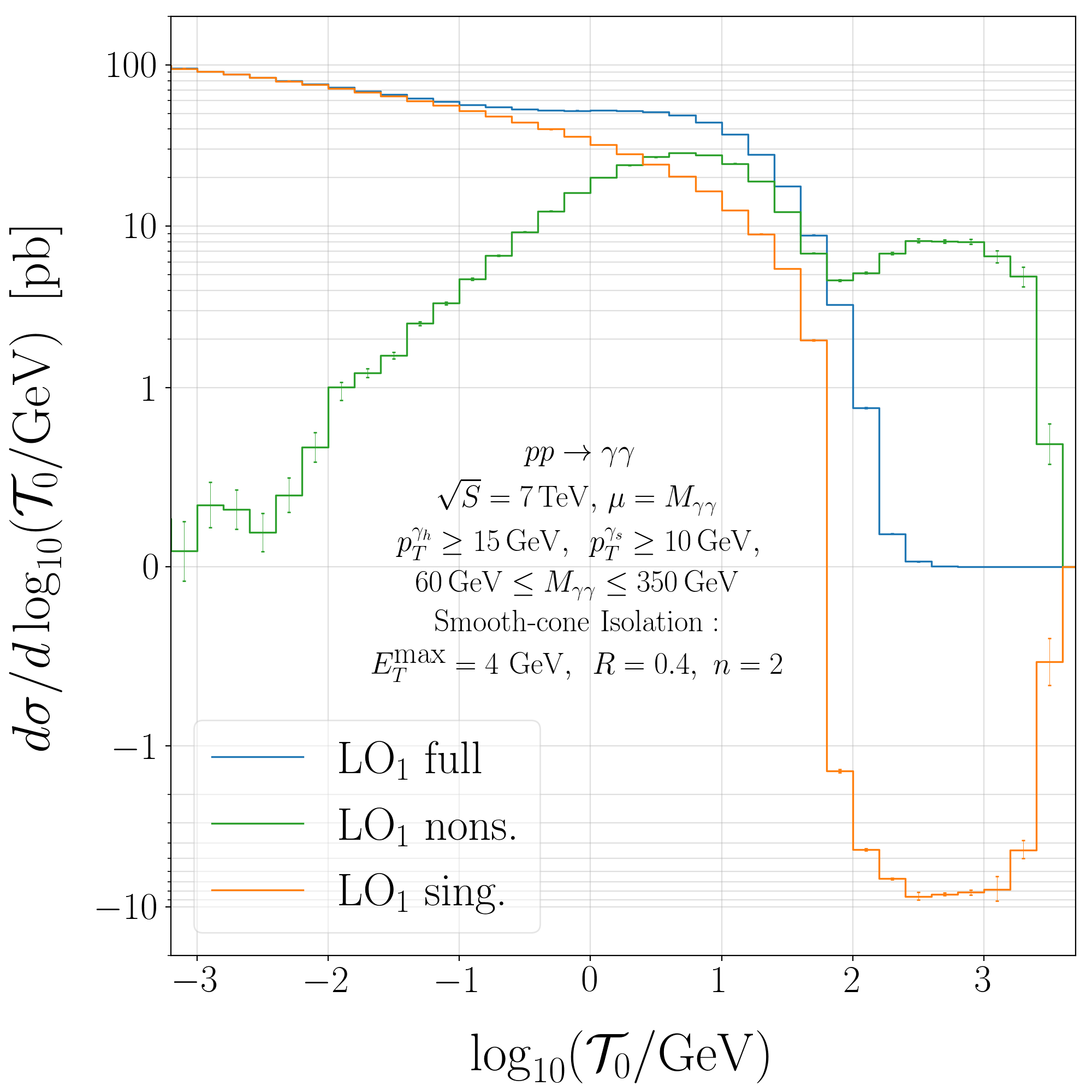
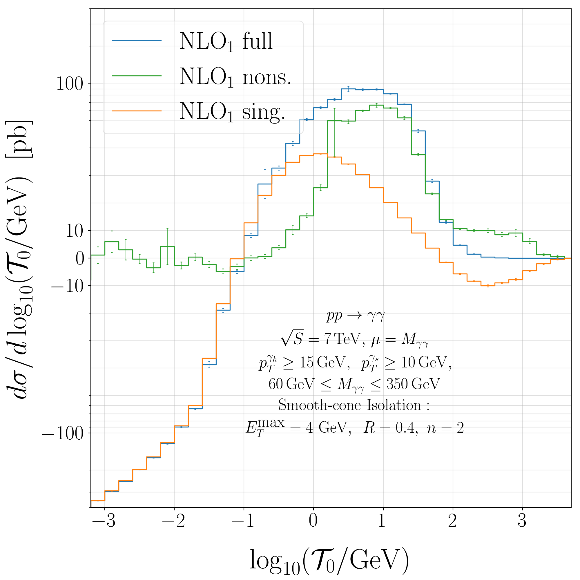
Figure 1: Singular and nonsingular contributions to the diphoton production cross section as a function of $\mathcal{T}_{0}$ at NLO (left) and NNLO (right).

In Fig. 1 we perform this comparison at different fixed orders. In both panels we show the FO calculation, the leading singular terms from the expansion of the resummed formula to the relevant fixed order and the difference between the two. The latter amounts to a nonsingular contribution to the cross section in the limit $\mathcal{T}_{0}\to 0$. As expected from the leading-power factorisation formula, each resummed-expanded contribution perfectly reproduces the singular behaviour of the corresponding FO term and acts as a subtraction to remove the IR divergences. Indeed, the nonsingular contributions vanish on a logarithmic scale as $\mathcal{T}_{0}\to 0$. One may also notice that the nonsingular terms become of similar size to the singular contributions at small values of $\mathcal{T}_{0}$, in the range of a few GeV. This behaviour is something of a novelty compared to the previous Drell–Yan and $VH$ production calculations and appears to be peculiar to the diphoton production process. Although the nonsingular terms are power suppressed for small $\mathcal{T}_{0}$ values, the photon isolation procedure might become the primary source of power corrections, enhancing their contribution and making them numerically large Ebert:2019zkb ; Balsiger:2018ezi ; Becher:2020ugp ; Wiesemann:2020gbm .

Resummation is carried out via RGE evolution and can be switched off by setting all of the scales equal to a common nonsingular scale $\mu_{\mathrm{NS}}=\mu_{S}=\mu_{B}=\mu_{H}$. We do not evolve the hard function, which is always evaluated at $\mu_{H}=\mu_{\mathrm{NS}}$ Ligeti:2008ac ; Abbate:2010xh . Instead we evolve the soft and the beam functions from their characteristic scales up to the hard scale. This is achieved by employing profile scales $\mu_{B}(\mathcal{T}_{0})$ and $\mu_{S}(\mathcal{T}_{0})$ which ensure a smooth transition between the resummation and the FO regimes. Explicitly,

$$\mu_{H} =\mu_{\mathrm{NS}}\,,$$

$$\mu_{S}(\mathcal{T}_{0}) =\mu_{\mathrm{NS}}\ f_{\rm run}(\mathcal{T}_{0}/Q)\,,$$

$$\mu_{B}(\mathcal{T}_{0}) =\mu_{\mathrm{NS}}\ \sqrt{f_{\rm run}(\mathcal{T}_{0}/Q)}\,,$$ (25)

where the common profile function $f_{\rm run}(x)$ is given by Stewart:2013faa

$$f_{\rm run}(x) =\begin{cases}x_{0}\bigl{[}1+(x/x_{0})^{2}/4\bigr{]}&x\leq 2x_{0}\,,\\ x&2x_{0}\leq x\leq x_{1}\,,\\ x+\frac{(2-x_{2}-x_{3})(x-x_{1})^{2}}{2(x_{2}-x_{1})(x_{3}-x_{1})}&x_{1}\leq x\leq x_{2}\,,\\ 1-\frac{(2-x_{1}-x_{2})(x-x_{3})^{2}}{2(x_{3}-x_{1})(x_{3}-x_{2})}&x_{2}\leq x\leq x_{3}\,,\\ 1&x_{3}\leq x\,.\end{cases}$$ (26)

This functional form ensures the canonical scaling behaviour as in eq. (9) for values below $x_{1}$ and turns off resummation above $x_{3}$. After considering that the invariant mass distribution peaks in the range $50$-$80$ GeV (depending on the specific cuts that are applied) and that the nonsingular corrections in Fig. 1 become of the same size of the singular at $\mathcal{T}_{0}\sim 1-3$ GeV, we choose the following parameters for the profile functions:

$$x_{0}=2.5\,\mathrm{GeV}/Q\,,\quad\{x_{1},x_{2},x_{3}\}=\{0.1,0.5,0.8\}\,.$$ (27)

In the resummation region the nonsingular scale $\mu_{\mathrm{NS}}$ must be of the same order as the hard scale of the process $M_{\gamma\gamma}$, while in the FO region it can be chosen to be any fixed or dynamical scale $\mu_{\mathrm{FO}}$. One can, for example, set it either to $M_{\gamma\gamma}$ or to the transverse mass of the photon pair $M^{T}_{\gamma\gamma}$.

We estimate the theoretical uncertainties for the FO predictions by varying the central choice for $\mu_{\mathrm{NS}}$ up and down by a factor of two and take for each observable the maximal absolute deviation from the central result as the FO uncertainty. For the resummation uncertainties, we vary the central choices for the profile scales $\mu_{B}$ and $\mu_{S}$ independently while keeping $\mu_{H}=\mu_{\mathrm{NS}}$ fixed. This gives us four independent variations. In addition, we consider two more profile functions where we shift all the $x_{i}$ transition points together by $\pm 0.05$ while keeping all of the scales fixed at their central values. Hence we obtain in total six profile variations. We consider the maximal absolute deviation in the results with respect to the central prediction as the resummation uncertainty. The total perturbative uncertainty is then calculated by adding the FO and the resummation uncertainties in quadrature.

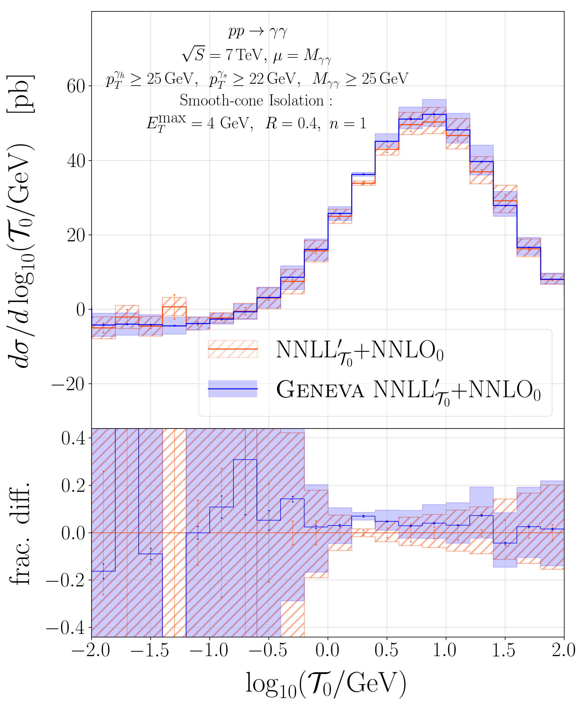
Figure 2: Comparison between standard resummation and event generation in Geneva in the presence of projection cuts. We show the resummed contribution alone (left) and the result matched to NNLO (right).

As explained in detail in Refs. Alioli:2015toa ; Alioli:2019qzz , the $\mathcal{T}_{0}$ integration of the resummation formula (eq. (3)) and the procedure of choosing the scales are operations which do not commute with each other. The expression for the cumulant is not, therefore, exactly the same as the integral of the $\mathcal{T}_{0}$ spectrum, since the profile scales have a functional dependence on $\mathcal{T}_{0}$. To obtain an expression for the resummed cumulant instead, one must first integrate the expression in eq. (3) for the resummed $\mathcal{T}_{0}$ distribution and then choose the scales using the same profile scales but with the $\mathcal{T}_{0}$ replaced by $\mathcal{T}^{\mathrm{cut}}_{0}$. For example the canonical scales assume the values

$$\mu_{H}=Q,\quad\quad\mu_{B}=\sqrt{Q\mathcal{T}^{\mathrm{cut}}_{0}},\quad\quad\mu_{S}=\mathcal{T}^{\mathrm{cut}}_{0}\,.$$ (28)

The difference between the two results for inclusive quantities is formally beyond NNLL^′ accuracy Almeida:2014uva . However, the numerical effect can be large and, in order to preserve the value of the NNLO₀ cross section, we follow the prescription for fully inclusive quantities discussed in Refs. Alioli:2015toa ; Alioli:2019qzz which amounts to adding the contribution

$$\kappa(\mathcal{T}_{0})\left[\frac{\mathrm{d}}{\mathrm{d}\mathcal{T}_{0}}\frac{\mathrm{d}\sigma^{\rm NNLL^{\prime}}}{\mathrm{d}\Phi_{0}}(\mathcal{T}_{0},\mu_{h}(\mathcal{T}_{0}))-\frac{\mathrm{d}\sigma^{\rm NNLL^{\prime}}}{\mathrm{d}\Phi_{0}\mathrm{d}\mathcal{T}_{0}}(\mu_{h}(\mathcal{T}_{0}))\right],$$ (29)

where $\kappa(\mathcal{T}_{0})$ and $\mu_{h}(\mathcal{T}_{0})$ are smooth functions. The $\mu_{h}(\mathcal{T}_{0})$ are new profile scales which are chosen to turn off resummation earlier than the normal profile scales in the resummed calculation, in order to maintain the accurate description of the tail of the $\mathcal{T}_{0}$ spectrum. Indeed, in the FO region we have that $\mu_{h}(\mathcal{T}_{0})=Q$ and the difference in the brackets of eq. (29) is zero, since it is proportional to $\mathrm{d}\mu_{h}/\mathrm{d}\mathcal{T}_{0}$. The $\kappa(\mathcal{T}_{0})$ function interpolates from a constant $\mathcal{O}(1)$ value at $\mathcal{T}_{0}\ll Q$ reaching zero when $\mu_{h}(\mathcal{T}_{0})=Q$. The value of $\kappa(\mathcal{T}_{0}\to 0)$ can be tuned such that after integration of the $\mathcal{T}_{0}$ spectrum together with eq. (29), the correct inclusive cross section is obtained. A more detailed explanation on the precise structure of this additional term can be found in Refs. Alioli:2015toa ; Alioli:2019qzz .

4.3 Comparison with standard resummation and matching

The implementation of resummation in the Geneva framework takes a very different perspective compared to the usual resummation approach. The latter is normally carried out with the purpose of improving the description of a single particular observable in the limit where it approaches very small or very large values compared to other scales present in the process. In practice, this involves a scan over the $\mathcal{T}_{0}$ spectrum by directly evaluating the resummation formula (eq. (3)) on a $\Phi_{0}$ phase space point. Hence the information about the physical event which generates a particular value of the resummed variable is not retained in the calculation. In an event generator such as Geneva, however, one starts by generating e.g. $\Phi_{1}$ events and calculating the value of the resummed variable, in this case $\mathcal{T}_{0}$, resulting from that particular event configuration. At this point one has to perform a projection to the lower-multiplicity phase space to evaluate the resummation formula. This second method is more flexible because it allows one to access the event information in a fully differential way and to associate to each event a resummed weight, also allowing the matching to a FO calculation.

Infrared safety ensures that even in the presence of process-defining cuts, which are applied either to $\Phi_{0}$ in the standard resummation or to $\Phi_{1}$ in Geneva, these two approaches are identical in the limit $\mathcal{T}_{0}\to 0$. Away from the limit, the two procedures will give the same result only if the quantities upon which the cuts are imposed are preserved by the $\Phi_{1}\to\Phi_{0}$ projection. For the Drell–Yan and $VH$ production processes previously studied in Geneva, the only process-defining cut was applied on the invariant mass of the colour-singlet system. Since this quantity was preserved by every projection, the problem was avoided. In the case of diphoton production instead, the $p_{T}$ cuts on each photon are not preserved by our mappings. Hence, these cuts applied to the projected $\widetilde{\Phi}_{0}$ configurations will effectively remove some contributions to the resummed and resummed-expanded terms of the cross section formula in eq. (4.1) which are present in the usual resummed results (i.e. without any recoil considered).

The difference between the two procedures is shown in the left plot of Fig. 2 for the resummed contribution alone, while the right plot shows the same comparison after matching to fixed order. We observe good compatibility between the two curves even at large $\mathcal{T}_{0}$, meaning that the difference between the two approaches is eliminated at FO by the matching procedure. We also observe larger fluctuations of the standard result at small $\mathcal{T}_{0}$ values, likely due to combining the histogram bins of the matched calculation rather than combining the contributions on an event-by-event basis as is done in Geneva.

We are now in a position to compare the effects of the $\mathcal{T}_{0}$ resummation matched to FO calculations by evaluating the cross section formulae in eq. (4.1) and eq. (4.1) at different accuracies.

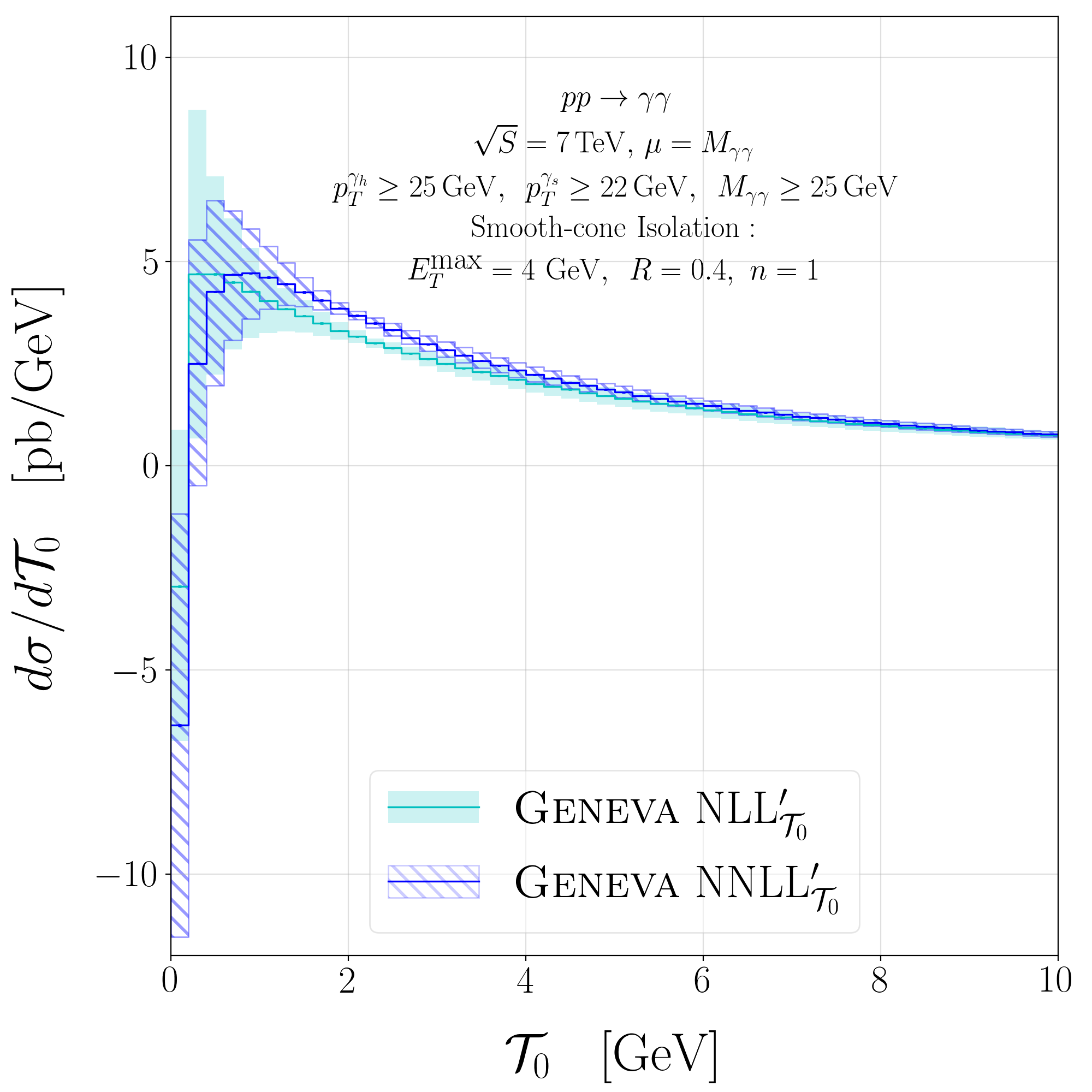
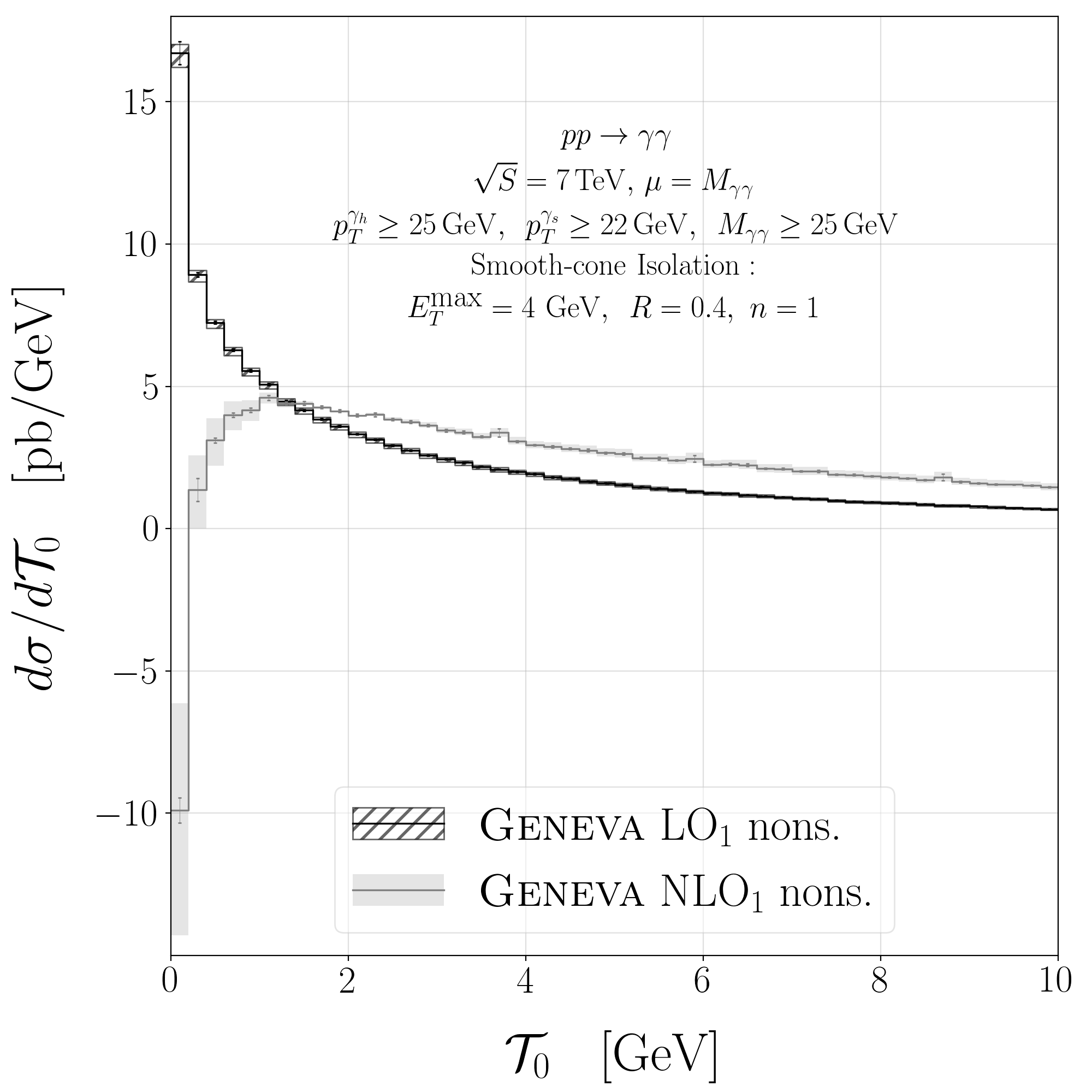
Figure 3: Comparison between the NLL^′ and NNLL^′ resummed $\mathcal{T}_{0}$ distributions in the peak region (left) and the corresponding nonsingular contribution (right).

In the left panel of Fig. 3 we compare the NLL^′ and NNLL^′ results for the $\mathcal{T}_{0}$ distribution in the peak region. In the same figure we also show the nonsingular contribution at NLO and NNLO in the same range of $\mathcal{T}_{0}$ on the right.

In the peak region, the two results at different resummation accuracies do overlap, but we do not observe a substantial reduction of the resummation uncertainties. We also notice that the nonsingular contribution at very small $\mathcal{T}_{0}$ values takes opposite signs at the different orders. Its size also looks particularly large when plotted on a linear scale, as is done in this plot (c.f. Fig. 1).

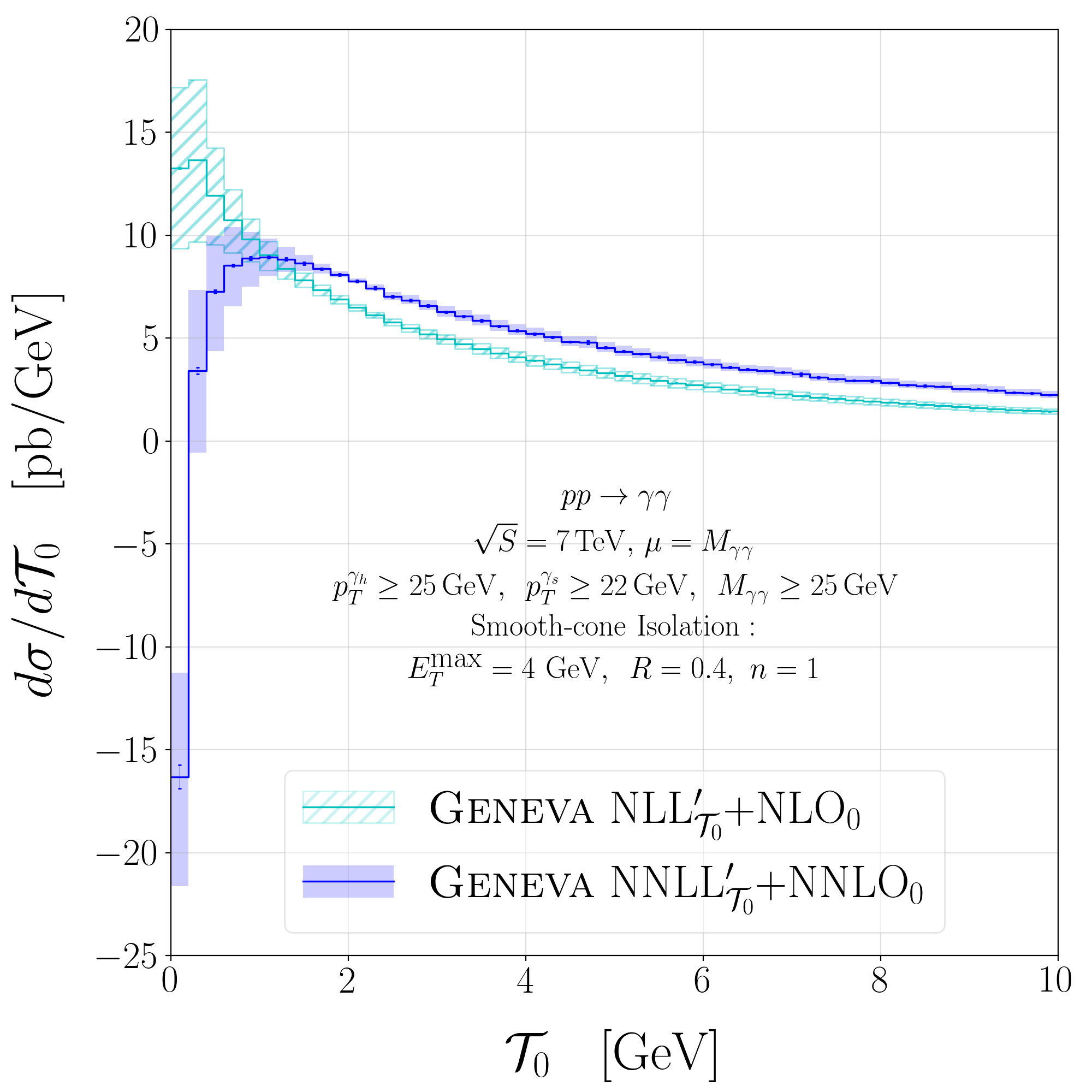
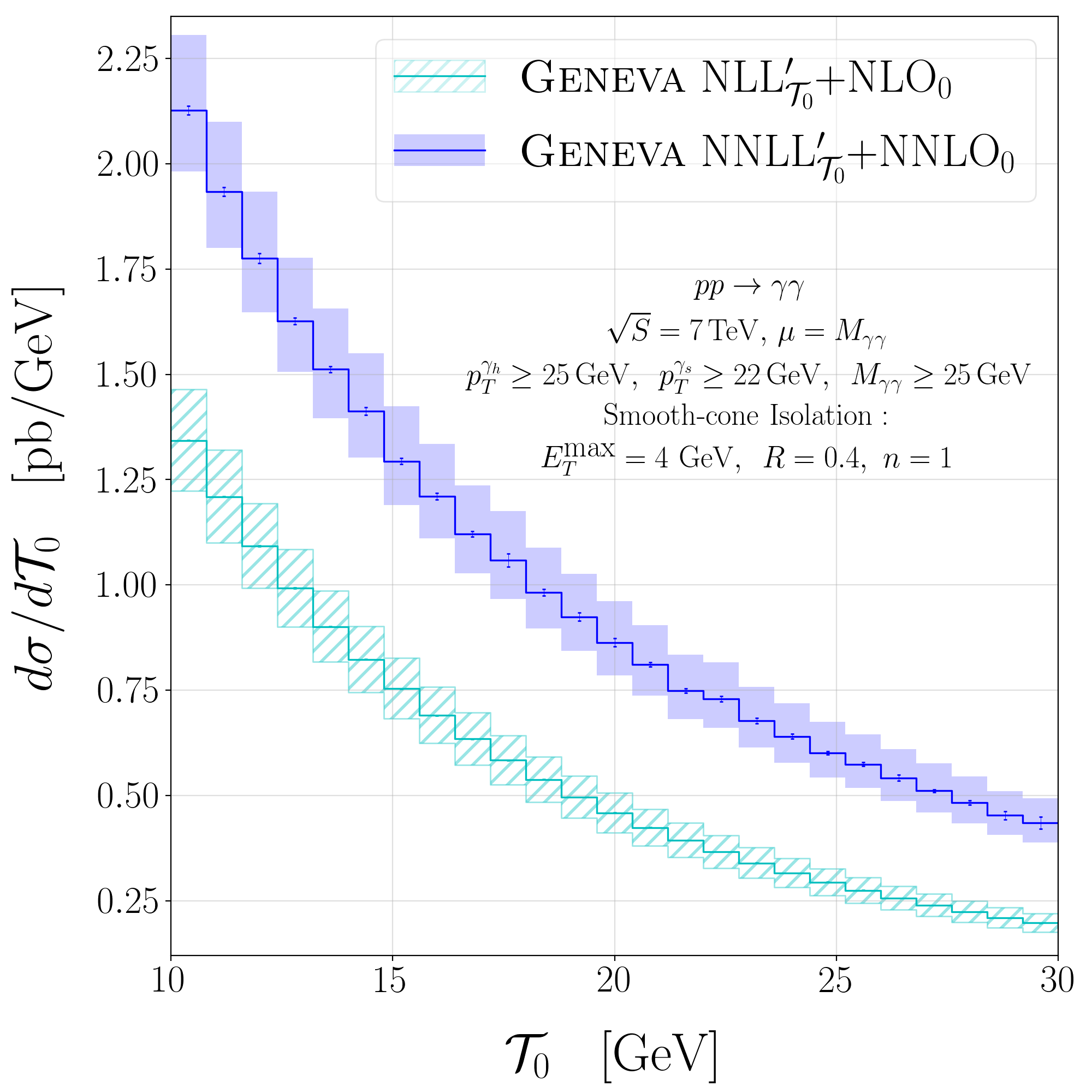
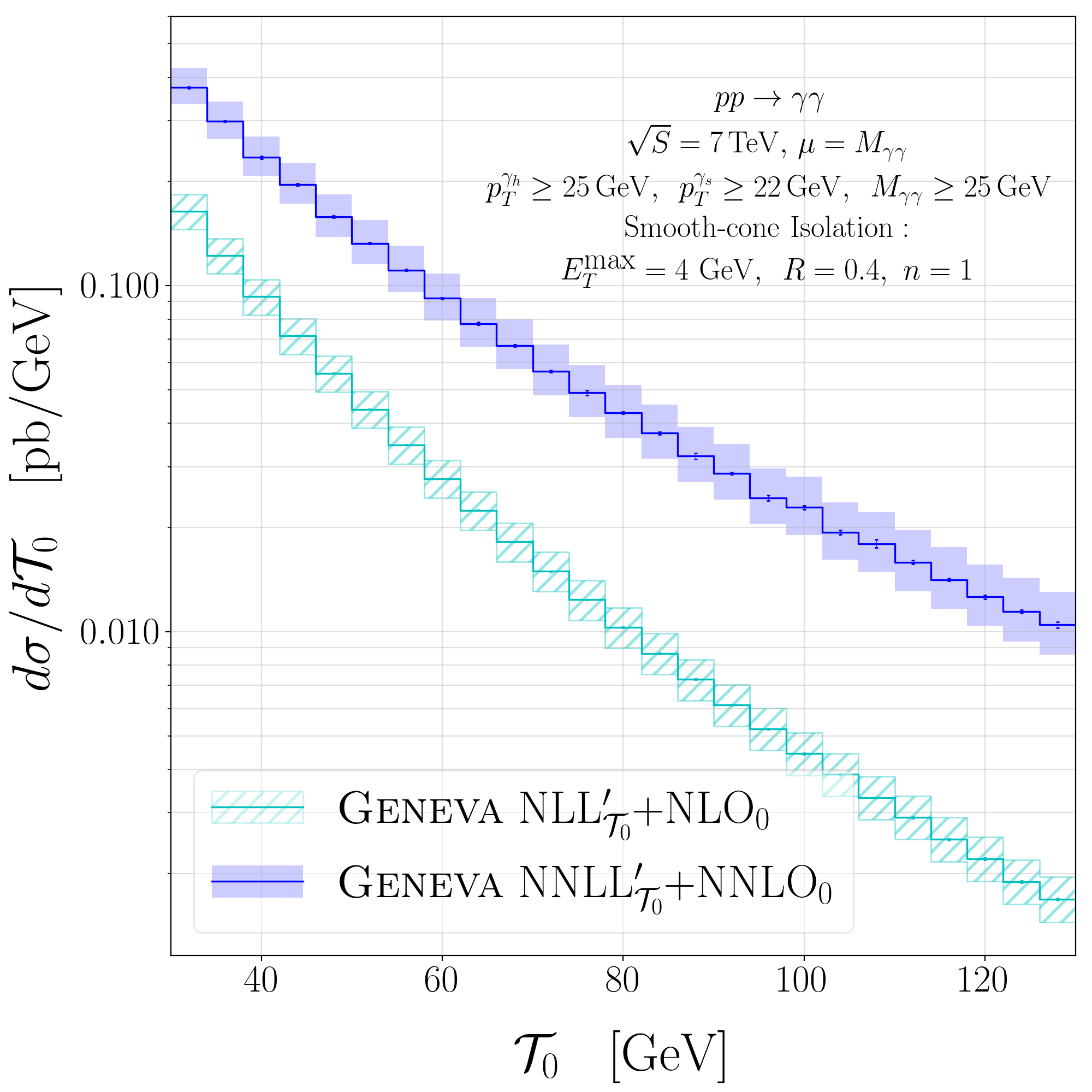
Figure 4: Comparison between the NLL^′+NLO and NNLL^′+NNLO matched $\mathcal{T}_{0}$ distributions in the peak (left), transition (centre) and tail (right) regions.

In Fig. 4 we instead plot the same resummed results matched to the appropriate FO calculation, in the peak, transition and tail regions. As a consequence of the size of the nonsingular corrections, the two curves only partially overlap for $1<\mathcal{T}_{0}<2$ GeV, close to the peak. A similarly poor convergence was also observed for the $p^{\gamma\gamma}_{T}$ distribution after performing the $q_{T}$ resummation (see Ref. Cieri:2015rqa ). Also in the tail and transition regions, the effect of including the NNLO corrections is large and the uncertainty bands do not overlap with those at lower order. This was previously noticed in Refs. Catani:2011qz ; Catani:2018krb ; Campbell:2016yrh .

4.4 Subleading power corrections

In order to express the 0-jet cross section as in eq. (4.1), i.e. fully differential in the $\Phi_{0}$ phase space one would need to implement a local NNLO subtraction method. However, if power corrections below the resolution cutoff are kept negligible by a careful choice of the cutoff, a local subtraction is not explicitly needed. This is the case of the Geneva approach, which is based on the $N$-jettiness subtraction Boughezal:2015dva ; Gaunt:2015pea .

Moreover, even if a local subtraction were provided, the predictions of an event generator would be inherently correct only for the total cross section and for observables which are left unchanged by the $\Phi_{1}\to\Phi_{0}$ and $\Phi_{2}\to\Phi_{1}\to\Phi_{0}$ projections like, for example, the diphoton invariant mass. Hence, the presence of power corrections in $\mathcal{T}^{\mathrm{cut}}_{0}$ cannot be avoided for generic observables that depend on the $\Phi_{0}$ kinematics. We therefore replace the formula for the 0-jet cross section in eq. (4.1) with

$$\frac{\widetilde{\mathrm{d}\sigma^{\textsc{mc}}_{0}}}{\mathrm{d}\Phi_{0}}(\mathcal{T}_{0}^{\mathrm{cut}})= \;\frac{\mathrm{d}\sigma^{\rm NNLL^{\prime}}}{\mathrm{d}\Phi_{0}}(\mathcal{T}_{0}^{\mathrm{cut}})\,-\biggl{[}\frac{\mathrm{d}\sigma^{\rm NNLL^{\prime}}}{\mathrm{d}\Phi_{0}}(\mathcal{T}_{0}^{\mathrm{cut}})\biggr{]}_{\rm NLO_{0}}$$

$$+(B_{0}+V_{0})(\Phi_{0})\,\Theta^{\mathrm{PS}}(\Phi_{0})\,$$

$$+\int\frac{\mathrm{d}\Phi_{1}}{\mathrm{d}\Phi_{0}}\,\,B_{1}(\Phi_{1})\,\Theta^{\mathrm{PS}}(\Phi_{1})\,\Theta^{\mathrm{proj}}(\widetilde{\Phi}_{0})\,\theta\big{(}\mathcal{T}_{0}(\Phi_{1})<\mathcal{T}_{0}^{\mathrm{cut}}\big{)}\,,$$ (30)

where the local subtraction and the expansion of the resummation formula are only needed up to $\mathcal{O}(\alpha_{s})$. This formula assumes that there is an exact cancellation between the FO and the resummed-expanded contribution at $\mathcal{O}(\alpha^{2}_{s})$ below the $\mathcal{T}^{\mathrm{cut}}_{0}$. This holds for the singular contributions due to the NNLL^′ accuracy of our resummation formula. However, this formula is only accurate at leading power in the SCET expansion parameter and fails to capture the nonsingular contributions in $\mathcal{T}^{\mathrm{cut}}_{0}$. These can be expressed as

$$\frac{\mathrm{d}\sigma_{0}^{\mathrm{nons}}}{\mathrm{d}\Phi_{0}}(\mathcal{T}_{0}^{\mathrm{cut}}) =\bigl{[}\alpha_{\rm s}f_{1}(\mathcal{T}_{0}^{\mathrm{cut}},\Phi_{0})+\alpha_{\rm s}^{2}f_{2}(\mathcal{T}_{0}^{\mathrm{cut}},\Phi_{0})\bigr{]}\,\mathcal{T}_{0}^{\mathrm{cut}}\,,$$ (31)

while their integral over the phase space can be written as

$$\Sigma_{\mathrm{ns}}(\mathcal{T}_{0}^{\mathrm{cut}}) =\int\mathrm{d}\Phi_{0}\,\frac{\mathrm{d}\sigma_{0}^{\mathrm{nons}}}{\mathrm{d}\Phi_{0}}(\mathcal{T}_{0}^{\mathrm{cut}})\,.$$ (32)

Since the functions $f_{i}(\mathcal{T}_{0}^{\mathrm{cut}},\Phi_{0})$ contain at worst logarithmic divergences, the nonsingular cumulant vanishes in the limit $\mathcal{T}_{0}^{\mathrm{cut}}\to 0$. In our calculation we include the term $f_{1}(\mathcal{T}_{0}^{\mathrm{cut}},\Phi_{0})$ exactly by means of the NLO₁ FKS local subtraction. The $f_{2}(\mathcal{T}_{0}^{\mathrm{cut}},\Phi_{0})$ term is instead completely neglected in eq. (31). This is acceptable as long as we choose $\mathcal{T}_{0}^{\mathrm{cut}}$ to be very small.

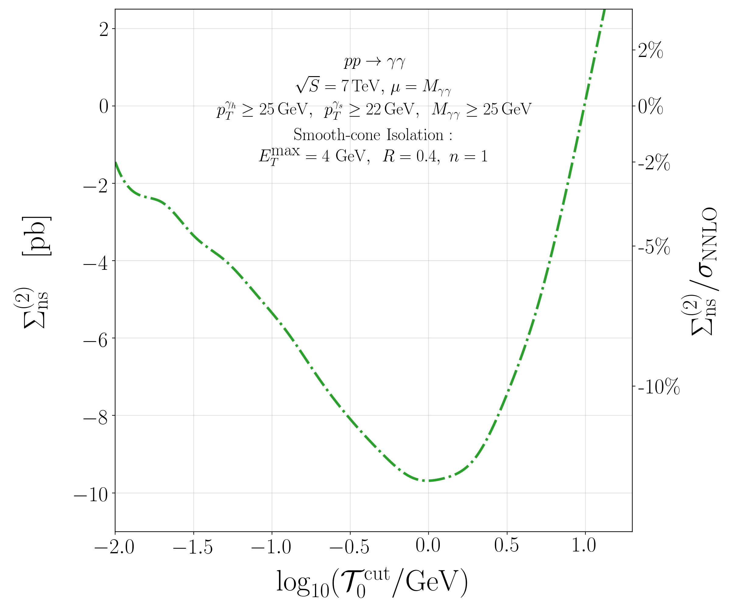
Figure 5: The neglected $\mathcal{O}(\alpha^{2}_{s})$ nonsingular contribution to the $\mathcal{T}_{0}$ cumulant, $\Sigma_{\mathrm{ns}}^{(2)}$, as a function of $\mathcal{T}^{\mathrm{cut}}_{0}$.

The effect of our approximation is shown in Fig. 5, where we plot the size of the neglected pure $\mathcal{O}(\alpha_{\rm s}^{2})$ terms in $\Sigma_{\mathrm{ns}}(\mathcal{T}_{0}^{\mathrm{cut}})$ as a function of $\mathcal{T}^{\mathrm{cut}}_{0}$. The size of the missing contributions is not completely negligible and to reduce their impact we run with a default cut value of $\mathcal{T}^{\mathrm{cut}}_{0}=0.01$ GeV. The magnitude of the missing corrections for such value of the cut is around $1.45$ pb (which corresponds to $\sim 2\%$ of the total cross section for the particular set of cuts chosen). Comparing this result to the previous Drell–Yan and $VH$ calculations, we notice that in the diphoton case the relative size of the nonsingular corrections below the cut is larger.

One could improve on this by systematically calculating the subleading terms in the expansion parameter using a SCET formalism. Presently, only the first terms in the expansion are known, for a limited set of processes Moult:2016fqy ; Boughezal:2016zws ; Moult:2017jsg .

We eventually provide the missing nonsingular $\mathcal{O}(\alpha^{2}_{s})$ contributions from an independent NNLO calculation obtained with Matrix Grazzini:2017mhc , by simply rescaling the weights of the $\Phi_{0}$ events by the cross section ratios. We remind the reader that the Matrix calculation is based on the $q_{T}$ subtraction method, which is very similar in spirit to $0$-jettiness subtraction and thus in principle affected by the same issue. However, Matrix uses an extrapolation procedure for $q^{\mathrm{cut}}_{T}\to 0$ which provides an estimate of the cross section and its numerical error. Therefore, reweighting the $\Phi_{0}$ events using the total cross section inputs from Matrix provides us with NNLO accuracy.

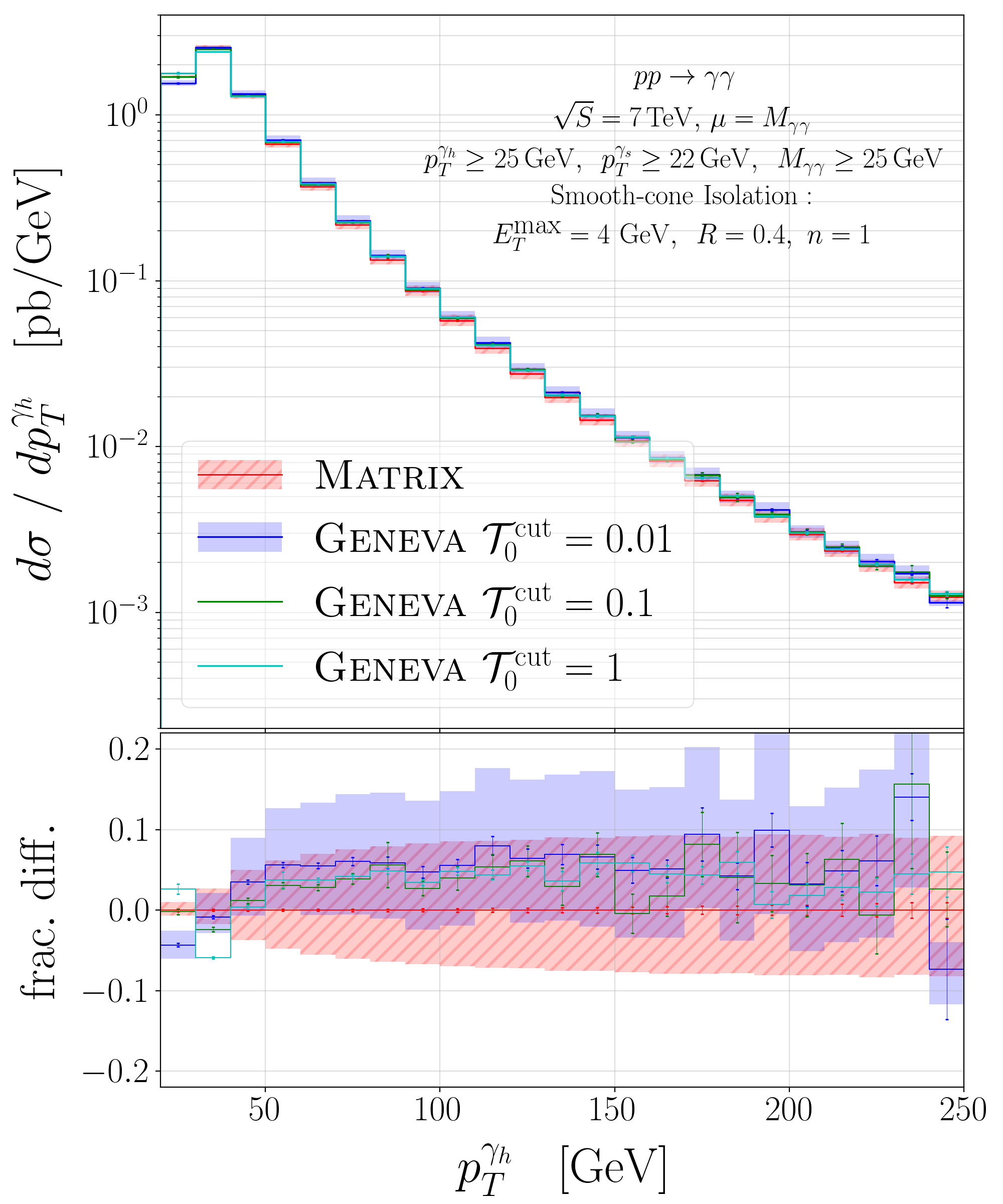
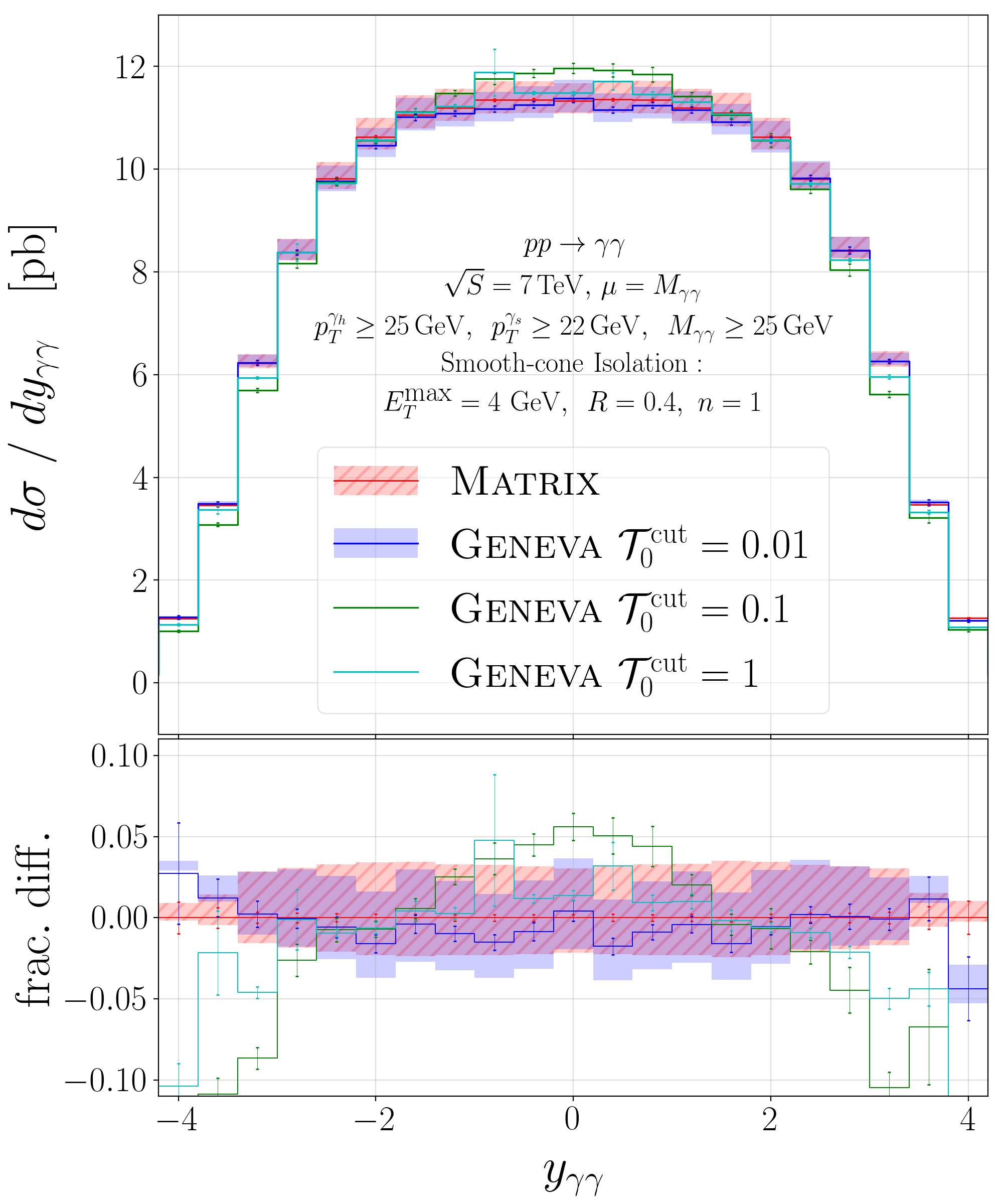
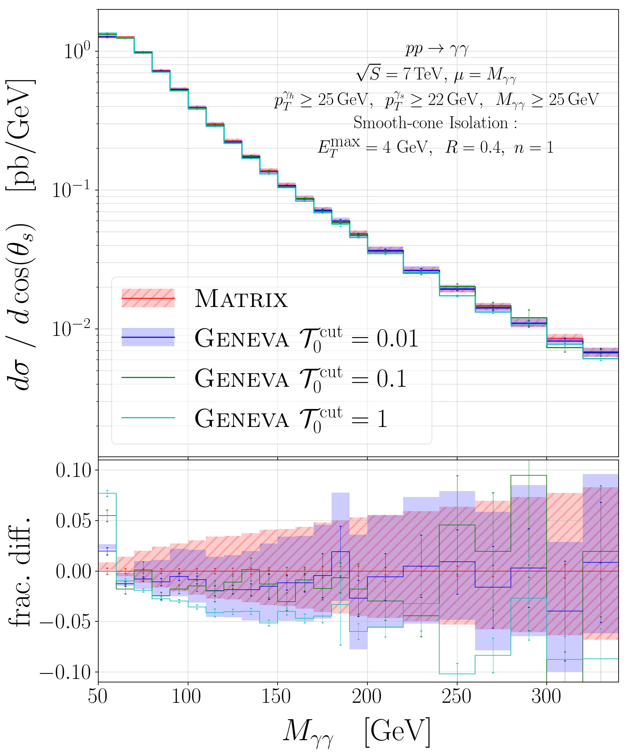
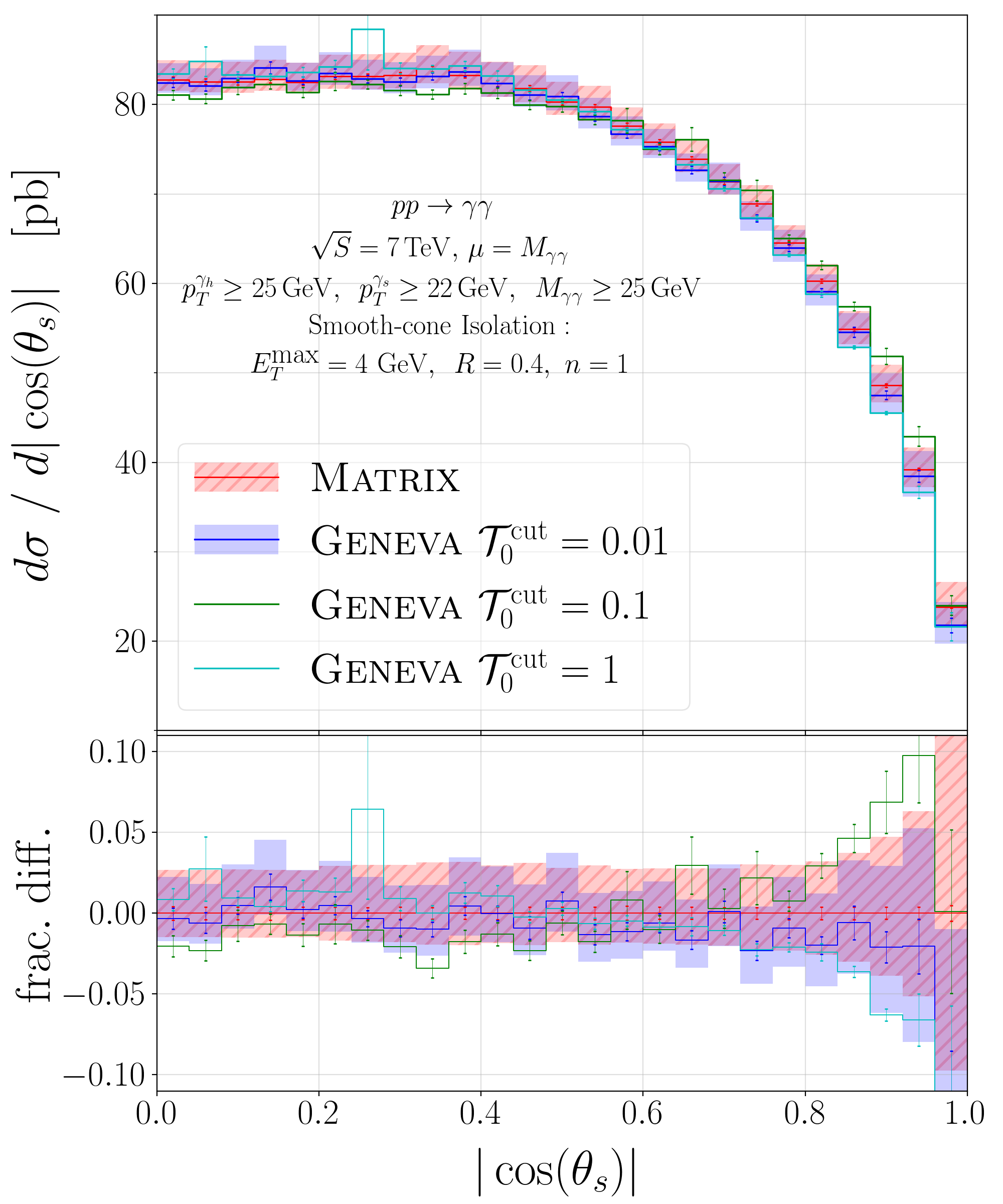
Figure 6: Comparison between Matrix and Geneva for different values of $\mathcal{T}^{\mathrm{cut}}_{0}$. We show the transverse momentum of the hardest photon (top left), rapidity of the diphoton system (top right), invariant mass of the diphoton system (bottom left) and the cosine of the photon scattering angle (bottom right).

4.5 NNLO validation

After reweighting the $\Phi_{0}$ events for the central scale choice as well as for its variations, we compare the inclusive (i.e. not probing additional radiation) distributions obtained with Geneva to the independent NNLO results obtained with Matrix Grazzini:2017mhc . This check is nontrivial since the complete dependence on the $\Phi_{0}$ kinematics is not, in general, captured by the reweighting.

In Fig. 6 we show the transverse momentum of the hardest photon, the rapidity and the invariant mass of the diphoton system, and the absolute value of the cosine of the photon scattering angle in the frame of the LO partonic collision, defined as

$$|\cos\theta_{s}|=\tanh\bigg{(}\frac{|\Delta y_{\gamma\gamma}|}{2}\bigg{)}\,,$$ (33)

where $\Delta y_{\gamma\gamma}$ is the diphoton rapidity separation. After comparing three different choices of $\mathcal{T}^{\mathrm{cut}}_{0}=\{0.01,0.1,1\}\,\,\mathrm{GeV}$ in Geneva we conclude that the best agreement with the NNLO predictions for these inclusive distributions is obtained for $\mathcal{T}^{\mathrm{cut}}_{0}=0.01$ GeV, as expected from the study of the missing power corrections (see sec. 4.4). We therefore set $\mathcal{T}^{\mathrm{cut}}_{0}$ to this default value for all of our predictions.

As mentioned above, the Geneva predictions, despite being NNLO accurate, are not exactly equivalent to those of a NNLO calculation: indeed, they differ by power-suppressed terms as a consequence of the projective map which is used to define the $\Phi_{0}$ events and by higher-order resummation effects that are not completely removed even after the inclusion of the additional terms in eq. (29). Nevertheless, the agreement between Geneva and Matrix for the distributions in Fig. 6 is good, within the uncertainty bands of the two calculations (representing the 3-point $\mu_{r}$ and $\mu_{f}$ variations).

4.6 Resumming the 1-jet/2-jet separation at LL

In order to provide an event generator which is as flexible as possible, and thus also able to provide exclusive predictions for higher-multiplicity bins, we proceed with the separation of the inclusive $1$-jet cross section into an exclusive $1$-jet cross section and an inclusive $2$-jet cross section. We can achieve this separation by using the $\mathcal{T}_{1}$ resolution variable. This introduces a new scale which in principle requires a simultaneous resummation of all the different ratios between the scales $\mathcal{T}_{0}$, $\mathcal{T}_{1}$ and $Q$, in all the possible kinematic regions. A fully satisfactory treatment of this kind is still lacking, but, in the region $\mathcal{T}_{1}\ll\mathcal{T}_{0}$, we can take the simpler approach explained next. We concentrate first on the $\mathcal{T}_{1}$ resummation and start by separating

$$\frac{\mathrm{d}\sigma^{\textsc{mc}}_{1}}{\mathrm{d}\Phi_{1}}(\mathcal{T}_{0}>\mathcal{T}_{0}^{\mathrm{cut}};\mathcal{T}_{1}^{\mathrm{cut}})= \;\frac{\mathrm{d}\sigma_{1}^{\rm LL}}{\mathrm{d}\Phi_{1}}(\mathcal{T}_{0}>\mathcal{T}_{0}^{\mathrm{cut}};\mathcal{T}_{1}^{\mathrm{cut}})\,$$

$$\hskip 20.00003pt+\frac{\mathrm{d}\sigma_{1}^{\mathrm{match}}}{\mathrm{d}\Phi_{1}}(\mathcal{T}_{0}>\mathcal{T}_{0}^{\mathrm{cut}};\mathcal{T}_{1}^{\mathrm{cut}})\,,$$ (34)

$$\frac{\mathrm{d}\sigma^{\textsc{mc}}_{\geq 2}}{\mathrm{d}\Phi_{2}}(\mathcal{T}_{0}>\mathcal{T}_{0}^{\mathrm{cut}},\mathcal{T}_{1}>\mathcal{T}_{1}^{\mathrm{cut}})= \;\frac{\mathrm{d}\sigma^{\rm LL}_{\geq 2}}{\mathrm{d}\Phi_{2}}\big{(}\mathcal{T}_{0}>\mathcal{T}_{0}^{\mathrm{cut}},\mathcal{T}_{1}>\mathcal{T}_{1}^{\mathrm{cut}}\big{)}\,$$

$$\hskip 20.00003pt+\frac{\mathrm{d}\sigma^{\mathrm{match}}_{\geq 2}}{\mathrm{d}\Phi_{2}}(\mathcal{T}_{0}>\mathcal{T}_{0}^{\mathrm{cut}},\mathcal{T}_{1}>\mathcal{T}_{1}^{\mathrm{cut}})\,,$$ (35)

where the terms $\mathrm{d}\sigma_{1}^{\rm LL}$ and $\mathrm{d}\sigma^{\rm LL}_{\geq 2}$ contain the LL resummation of the $\mathcal{T}_{1}^{\mathrm{cut}}$ and $\mathcal{T}_{1}$ dependencies respectively. The $\mathrm{d}\sigma_{1}^{\mathrm{match}}$ and $\mathrm{d}\sigma^{\mathrm{match}}_{\geq 2}$ terms contain the matching corrections to the required FO accuracy. At this point we can implement a unitary approach such that the resummed contributions take the form

$$\frac{\mathrm{d}\sigma_{1}^{\rm LL}}{\mathrm{d}\Phi_{1}}(\mathcal{T}_{0}>\mathcal{T}_{0}^{\mathrm{cut}};\mathcal{T}_{1}^{\mathrm{cut}})= \;\frac{\mathrm{d}\sigma_{\geq 1}^{C}}{\mathrm{d}\Phi_{1}}\,U_{1}(\Phi_{1},\mathcal{T}_{1}^{\mathrm{cut}})\,\Theta^{\mathrm{PS}}(\Phi_{1})\,\theta(\mathcal{T}_{0}>\mathcal{T}_{0}^{\mathrm{cut}})\,,$$ (36)

$$\frac{\mathrm{d}\sigma^{\rm LL}_{\geq 2}}{\mathrm{d}\Phi_{2}}(\mathcal{T}_{0}>\mathcal{T}_{0}^{\mathrm{cut}},\mathcal{T}_{1}>\mathcal{T}_{1}^{\mathrm{cut}})= \;\frac{\mathrm{d}\sigma_{\geq 1}^{C}}{\mathrm{d}\Phi_{1}}\,U_{1}^{\prime}(\widetilde{\Phi}_{1},\mathcal{T}_{1})\,\theta(\mathcal{T}_{0}>\mathcal{T}_{0}^{\mathrm{cut}})\Big{|}_{\widetilde{\Phi}_{1}=\Phi_{1}^{\mathcal{T}}(\Phi_{2})}\,$$

$$\hskip 30.00005pt\times\Theta^{\mathrm{PS}}(\Phi_{2})\,\Theta^{\mathrm{proj}}(\widetilde{\Phi}_{1})\,\mathcal{P}(\Phi_{2})\,\theta\left(\mathcal{T}_{1}>\mathcal{T}_{1}^{\mathrm{cut}}\right)\,.$$ (37)

The evolution function (or Sudakov factor) $U_{1}(\Phi_{1},\mathcal{T}_{1}^{\mathrm{cut}})$ resums the $\mathcal{T}_{1}^{\mathrm{cut}}$ dependence at LL accuracy in the region $\mathcal{T}_{1}^{\mathrm{cut}}\ll\mathcal{T}_{0}$, while $U_{1}^{\prime}(\Phi_{1},\mathcal{T}_{1})$ is the derivative of the evolution function with respect to $\mathcal{T}_{1}^{\mathrm{cut}}$. The latter resums the differential $\mathcal{T}_{1}$ dependence and is evaluated at the projected configuration $\widetilde{\Phi}_{1}=\Phi_{1}^{\mathcal{T}}(\Phi_{2})$. The function $\mathcal{P}(\Phi_{2})$ is a normalised splitting probability which is defined similarly to $\mathcal{P}(\Phi_{1})$ in eq. (17). The quantity $\mathrm{d}\sigma_{\geq 1}^{C}/\mathrm{d}\Phi_{1}$, which appears both in eqs. (36) and (4.6), is the inclusive 1-jet cross section in the singular $\mathcal{T}_{1}\to 0$ limit. Its NLO₁ expansion is given by

$$\biggl{[}\frac{\mathrm{d}\sigma^{C}_{\geq 1}}{\mathrm{d}\Phi_{1}}\biggr{]}_{\mathrm{NLO}_{1}}= \;\bigg{(}B_{1}(\Phi_{1})+V_{1}(\Phi_{1})+\int\!\frac{\mathrm{d}\Phi_{2}}{\mathrm{d}\Phi^{C}_{1}}\,C_{2}(\Phi_{2})\bigg{)}\,\Theta^{\mathrm{PS}}(\Phi_{1})\,$$

$$\equiv \;(B_{1}+V_{1}^{C})(\Phi_{1})\Theta^{\mathrm{PS}}(\Phi_{1})\,,$$ (38)

where $C_{2}(\Phi_{2})$ reproduces the point-wise singular behaviour of $B_{2}(\Phi_{2})$ and acts as a local subtraction at NLO Frixione:1995ms with its own projection $\mathrm{d}\Phi_{2}/\mathrm{d}\Phi^{C}_{1}\equiv\mathrm{d}\Phi_{2}\,\delta[\Phi_{1}-\Phi_{1}^{C}(\Phi_{2})]$. After requiring that $\mathrm{d}\sigma^{\textsc{mc}}_{1}$ and $\mathrm{d}\sigma^{\textsc{mc}}_{\geq 2}$ are accurate to NLO₁ and LO₂ respectively, the matching corrections are expressed as

$$\frac{\mathrm{d}\sigma_{1}^{\mathrm{match}}}{\mathrm{d}\Phi_{1}}(\mathcal{T}_{0}>\mathcal{T}_{0}^{\mathrm{cut}};\mathcal{T}_{1}^{\mathrm{cut}})= \;\frac{\mathrm{d}\sigma_{1}^{{\rm NLO_{1}}}}{\mathrm{d}\Phi_{1}}(\mathcal{T}_{0}>\mathcal{T}_{0}^{\mathrm{cut}};\mathcal{T}_{1}^{\mathrm{cut}})\,$$

$$\hskip 20.00003pt-\biggl{[}\frac{\mathrm{d}\sigma_{1}^{\rm LL}}{\mathrm{d}\Phi_{1}}(\mathcal{T}_{0}>\mathcal{T}_{0}^{\mathrm{cut}};\mathcal{T}_{1}^{\mathrm{cut}})\biggr{]}_{\rm NLO_{1}}\,,$$ (39)

$$\frac{\mathrm{d}\sigma_{\geq 2}^{\mathrm{match}}}{\mathrm{d}\Phi_{2}}(\mathcal{T}_{0}>\mathcal{T}_{0}^{\mathrm{cut}},\mathcal{T}_{1}>\mathcal{T}_{1}^{\mathrm{cut}})= \;\frac{\mathrm{d}\sigma_{\geq 2}^{{\rm LO_{2}}}}{\mathrm{d}\Phi_{2}}(\mathcal{T}_{0}>\mathcal{T}_{0}^{\mathrm{cut}},\mathcal{T}_{1}>\mathcal{T}_{1}^{\mathrm{cut}})\,$$

$$\hskip 20.00003pt-\biggl{[}\frac{\mathrm{d}\sigma_{\geq 2}^{\rm LL}}{\mathrm{d}\Phi_{2}}\left(\mathcal{T}_{0}>\mathcal{T}_{0}^{\mathrm{cut}},\mathcal{T}_{1}>\mathcal{T}_{1}^{\mathrm{cut}}\right)\biggr{]}_{\rm LO_{2}}\,.$$ (40)

After inserting eq. (36), eq. (4.6) and eq. (4.6) in the above equations and taking into account the appropriate phase space restrictions we find

$$\frac{\mathrm{d}\sigma_{1}^{\mathrm{match}}}{\mathrm{d}\Phi_{1}}(\mathcal{T}_{0}>\mathcal{T}_{0}^{\mathrm{cut}};\mathcal{T}_{1}^{\mathrm{cut}})= \int\ \biggl{[}\frac{\mathrm{d}\Phi_{2}}{\mathrm{d}\Phi^{\mathcal{T}}_{1}}\,B_{2}(\Phi_{2})\,\Theta^{\mathrm{PS}}(\Phi_{2})\,\theta\left(\mathcal{T}_{0}(\Phi_{2})>\mathcal{T}_{0}^{\mathrm{cut}}\right)\,\theta(\mathcal{T}_{1}<\mathcal{T}_{1}^{\mathrm{cut}})$$

$$-\frac{\mathrm{d}\Phi_{2}}{\mathrm{d}\Phi_{1}^{C}}\,C_{2}(\Phi_{2})\Theta^{\mathrm{PS}}(\Phi_{1})\,\theta(\mathcal{T}_{0}>\mathcal{T}_{0}^{\mathrm{cut}})\biggr{]}$$

$$-B_{1}(\Phi_{1})\,U_{1}^{(1)}(\Phi_{1},\mathcal{T}_{1}^{\mathrm{cut}})\,\Theta^{\mathrm{PS}}(\Phi_{1})\theta(\mathcal{T}_{0}>\mathcal{T}_{0}^{\mathrm{cut}})\,,$$ (41)

$$\frac{\mathrm{d}\sigma_{\geq 2}^{\mathrm{match}}}{\mathrm{d}\Phi_{2}}(\mathcal{T}_{0}>\mathcal{T}_{0}^{\mathrm{cut}},\mathcal{T}_{1}>\mathcal{T}_{1}^{\mathrm{cut}})= \;\Theta^{\mathrm{PS}}(\Phi_{2})\,\theta\left(\mathcal{T}_{0}(\Phi_{2})>\mathcal{T}_{0}^{\mathrm{cut}}\right)\,\big{[}B_{2}(\Phi_{2})\,\theta(\mathcal{T}_{1}>\mathcal{T}^{\mathrm{cut}}_{1})\,$$

$$-B_{1}(\Phi_{1}^{\mathcal{T}})\,U_{1}^{{(1)}\prime}(\widetilde{\Phi}_{1},\mathcal{T}_{1})\,\mathcal{P}(\Phi_{2})\,\Theta^{\mathrm{proj}}(\widetilde{\Phi}_{1})\,\theta(\mathcal{T}_{1}>\mathcal{T}_{1}^{\mathrm{cut}})\big{]}\,\,.$$ (42)

In the above expressions $U^{(1)}_{1}(\Phi_{1},\mathcal{T}^{\mathrm{cut}}_{1})$ and $U^{(1)\,\prime}_{1}(\Phi_{1},\mathcal{T}_{1})$ indicate the $\mathcal{O}(\alpha_{s})$ expansions of the evolution function $U_{1}(\Phi_{1},\mathcal{T}_{1}^{\mathrm{cut}})$ and of its derivative $U_{1}^{\prime}(\Phi_{1},\mathcal{T}_{1})$ respectively. Since the $\mathcal{T}_{1}$ resummation is carried out to LL accuracy, the matching corrections still contain subleading single-logarithmic terms.

So far we have presented a NLO₁+LL${}_{\mathcal{T}_{1}}$ matched result, but we still need to incorporate the $\mathcal{T}_{0}$ resummation that we discussed in the previous sections. We achieve this by requiring that the integral of the NLO₁+LL${}_{\mathcal{T}_{1}}$ result reproduces the $\mathcal{T}_{0}$-resummed result for the inclusive 1-jet MC cross section $\mathrm{d}\sigma^{\textsc{mc}}_{\geq 1}$

$$\frac{\mathrm{d}\sigma^{\textsc{mc}}_{\geq 1}}{\mathrm{d}\Phi_{1}}(\mathcal{T}_{0}>\mathcal{T}_{0}^{\mathrm{cut}})= \;\frac{\mathrm{d}\sigma^{\textsc{mc}}_{1}}{\mathrm{d}\Phi_{1}}(\mathcal{T}_{0}>\mathcal{T}_{0}^{\mathrm{cut}};\mathcal{T}_{1}^{\mathrm{cut}})+\int\!\frac{\mathrm{d}\Phi_{2}}{\mathrm{d}\Phi^{\mathcal{T}}_{1}}\,\frac{\mathrm{d}\sigma^{\textsc{mc}}_{\geq 2}}{\mathrm{d}\Phi_{2}}(\mathcal{T}_{0}>\mathcal{T}_{0}^{\mathrm{cut}},\mathcal{T}_{1}>\mathcal{T}_{1}^{\mathrm{cut}})\,.$$ (43)

The next step for the process at hand is nontrivial and requires some detailed explanation. In the case of Drell–Yan or $VH$ production, once this point was reached in the derivation one could simply proceed by summing the two contributions in the equation above. In this manner one could obtain a result which was independent of the evolution function, of its derivative and of the respective FO expansions, by exploiting the unitarity condition

$$U_{1}(\Phi_{1},\mathcal{T}_{1}^{\mathrm{cut}})+\int\!\frac{\mathrm{d}\Phi_{2}}{\mathrm{d}\Phi^{\mathcal{T}}_{1}}\,U_{1}^{\prime}(\Phi_{1},\mathcal{T}_{1})\,\mathcal{P}(\Phi_{2})\,\theta(\mathcal{T}_{1}>\mathcal{T}_{1}^{\mathrm{cut}})=1\,.$$ (44)

Unfortunately, in the case of diphoton production, this step is complicated by the presence of additional phase space restrictions on $\Phi_{2}$, due to the application of process-defining cuts, isolation cuts and projection cuts. Assuming that eq. (44) holds to to a good approximation despite the presence of all these cuts, we obtain

$$\frac{\mathrm{d}\sigma^{\textsc{mc}}_{\geq 1}}{\mathrm{d}\Phi_{1}}(\mathcal{T}_{0}>\mathcal{T}_{0}^{\mathrm{cut}})= \;\frac{\mathrm{d}\sigma_{\geq 1}^{C}}{\mathrm{d}\Phi_{1}}\,\theta(\mathcal{T}_{0}>\mathcal{T}_{0}^{\mathrm{cut}})+\int\!\bigg{[}\frac{\mathrm{d}\Phi_{2}}{\mathrm{d}\Phi^{\mathcal{T}}_{1}}\,B_{2}(\Phi_{2})\,\Theta^{\mathrm{PS}}(\Phi_{2})\,\theta\left(\mathcal{T}_{0}(\Phi_{2})>\mathcal{T}_{0}^{\mathrm{cut}}\right)\,$$

$$-\frac{\mathrm{d}\Phi_{2}}{\mathrm{d}\Phi_{1}^{C}}\,C_{2}(\Phi_{2})\,\Theta^{\mathrm{PS}}(\Phi_{1})\,\theta(\mathcal{T}_{0}>\mathcal{T}_{0}^{\mathrm{cut}})\bigg{]}+\ldots\,,$$ (45)

where the dots represent the remaining unitarity violating terms. We verified that, when implementing the $\mathcal{T}_{1}$ resummation at LL, these terms are indeed numerically small both for the total cross section and at the differential level for the $\mathcal{T}_{0}$ distribution. Therefore, we neglect them in the following. By comparing the expression on the r.h.s. of eq. (4.6) with the r.h.s. of eq. (4.1) we obtain the result for $\mathrm{d}\sigma_{\geq 1}^{C}$ ,

$$\frac{\mathrm{d}\sigma_{\geq 1}^{C}}{\mathrm{d}\Phi_{1}}(\mathcal{T}_{0}>\mathcal{T}_{0}^{\mathrm{cut}})= \;\Bigg{\{}\frac{\mathrm{d}\sigma^{\rm NNLL^{\prime}}}{\mathrm{d}\Phi_{0}\mathrm{d}\mathcal{T}_{0}}-\biggl{[}\frac{\mathrm{d}\sigma^{\rm NNLL^{\prime}}}{\mathrm{d}\Phi_{0}\mathrm{d}\mathcal{T}_{0}}\biggr{]}_{\rm NLO_{1}}\Bigg{\}}\,\mathcal{P}(\Phi_{1})\,\theta(\mathcal{T}_{0}>\mathcal{T}_{0}^{\mathrm{cut}})\,\Theta^{\mathrm{proj}}(\widetilde{\Phi}_{0})\,$$

$$+(B_{1}+V^{C}_{1})(\Phi_{1})\,\theta(\mathcal{T}_{0}(\Phi_{1})>\mathcal{T}^{\mathrm{cut}}_{0})\,.$$ (46)

Finally, we obtain the complete formulae for the exclusive 1-jet and the inclusive 2-jet cross sections as implemented in the Geneva code:

$$\frac{\mathrm{d}\sigma^{\textsc{mc}}_{1}}{\mathrm{d}\Phi_{1}}(\mathcal{T}_{0}\leq\mathcal{T}_{0}^{\mathrm{cut}};\mathcal{T}_{1}^{\mathrm{cut}})= \;\Theta^{\mathrm{PS}}(\Phi_{1})\,B_{1}\,(\Phi_{1})\,\theta(\mathcal{T}_{0}<\mathcal{T}^{\mathrm{cut}}_{0})\,\big{[}\overline{\Theta}_{\mathrm{iso}}^{\mathrm{proj}}(\widetilde{\Phi}_{0})+\overline{\Theta}^{\mathrm{FKS}}_{\mathrm{map}}(\Phi_{1})\big{]}\,,$$ (47)

$$\frac{\mathrm{d}\sigma^{\textsc{mc}}_{1}}{\mathrm{d}\Phi_{1}}(\mathcal{T}_{0}>\mathcal{T}_{0}^{\mathrm{cut}};\mathcal{T}_{1}^{\mathrm{cut}})= \;\Theta^{\mathrm{PS}}(\Phi_{1})\Bigg{\{}\Bigg{[}\frac{\mathrm{d}\sigma^{\rm NNLL^{\prime}}}{\mathrm{d}\Phi_{0}\mathrm{d}\mathcal{T}_{0}}-\frac{\mathrm{d}\sigma^{\rm NNLL^{\prime}}}{\mathrm{d}\Phi_{0}\mathrm{d}\mathcal{T}_{0}}\bigg{|}_{\mathrm{NLO}_{1}}\,\Bigg{]}\,\mathcal{P}(\Phi_{1})\,\Theta^{\mathrm{proj}}(\widetilde{\Phi}_{0})\,$$

$$\hskip 50.00008pt+\big{[}B_{1}+V_{1}^{C}\big{]}(\Phi_{1})\Bigg{\}}\times U_{1}(\Phi_{1},\mathcal{T}_{1}^{\mathrm{cut}})\,\theta(\mathcal{T}_{0}>\mathcal{T}_{0}^{\mathrm{cut}})$$

$$+\int\ \bigg{[}\frac{\mathrm{d}\Phi_{2}}{\mathrm{d}\Phi^{\mathcal{T}}_{1}}\,B_{2}(\Phi_{2})\,\Theta^{\mathrm{PS}}(\Phi_{2})\,\Theta^{\mathrm{proj}}(\widetilde{\Phi}_{1})\,\theta\left(\mathcal{T}_{0}(\Phi_{2})>\mathcal{T}_{0}^{\mathrm{cut}}\right)\,\theta(\mathcal{T}_{1}<\mathcal{T}_{1}^{\mathrm{cut}})\,$$

$$-\frac{\mathrm{d}\Phi_{2}}{\mathrm{d}\Phi^{C}_{1}}\,C_{2}(\Phi_{2})\,\Theta^{\mathrm{PS}}(\Phi_{1})\,\theta(\mathcal{T}_{0}>\mathcal{T}_{0}^{\mathrm{cut}})\bigg{]}\,$$

$$-B_{1}(\Phi_{1})\,U_{1}^{(1)}(\Phi_{1},\mathcal{T}_{1}^{\mathrm{cut}})\,\Theta^{\mathrm{PS}}(\Phi_{1})\,\theta(\mathcal{T}_{0}>\mathcal{T}_{0}^{\mathrm{cut}})\,,$$ (48)

$$\frac{\mathrm{d}\sigma^{\textsc{mc}}_{\geq 2}}{\mathrm{d}\Phi_{2}}(\mathcal{T}_{0}>\mathcal{T}_{0}^{\mathrm{cut}},\mathcal{T}_{1}\leq\mathcal{T}_{1}^{\mathrm{cut}})= \;B_{2}(\Phi_{2})\,\Theta^{\mathrm{PS}}(\Phi_{2})\,\Big{[}\overline{\Theta}_{\mathrm{map}}^{\mathcal{T}}(\Phi_{2})+\overline{\Theta}^{\mathrm{proj}}(\widetilde{\Phi}_{1})\Big{]}\,$$

$$\times\,\theta(\mathcal{T}_{1}<\mathcal{T}_{1}^{\mathrm{cut}})\,\theta\left(\mathcal{T}_{0}(\Phi_{2})>\mathcal{T}_{0}^{\mathrm{cut}}\right)\,,$$ (49)

$$\frac{\mathrm{d}\sigma^{\textsc{mc}}_{\geq 2}}{\mathrm{d}\Phi_{2}}(\mathcal{T}_{0}>\mathcal{T}_{0}^{\mathrm{cut}},\mathcal{T}_{1}>\mathcal{T}_{1}^{\mathrm{cut}})= \;\Theta^{\mathrm{PS}}(\Phi_{2})\,\Bigg{\{}\bigg{[}\frac{\mathrm{d}\sigma^{\rm NNLL^{\prime}}}{\mathrm{d}\Phi_{0}\mathrm{d}\mathcal{T}_{0}}-\frac{\mathrm{d}\sigma^{\rm NNLL^{\prime}}}{\mathrm{d}\Phi_{0}\mathrm{d}\mathcal{T}_{0}}\bigg{|}_{\mathrm{NLO}_{1}}\bigg{]}\,\mathcal{P}(\widetilde{\Phi}_{1})\,\Theta^{\mathrm{proj}}(\widetilde{\Phi}_{0})\,$$

$$+(B_{1}+V_{1}^{C})(\widetilde{\Phi}_{1})\Bigg{\}}\,U_{1}^{\prime}(\widetilde{\Phi}_{1},\mathcal{T}_{1})\,\theta(\mathcal{T}_{0}>\mathcal{T}_{0}^{\mathrm{cut}})\Big{|}_{\widetilde{\Phi}_{1}=\Phi_{1}^{\mathcal{T}}(\Phi_{2})}\!\!\,\Theta^{\mathrm{proj}}(\widetilde{\Phi}_{1})\mathcal{P}(\Phi_{2})\,\theta(\mathcal{T}_{1}>\mathcal{T}_{1}^{\mathrm{cut}})$$

$$+\Theta^{\mathrm{PS}}(\Phi_{2})\,\Big{\{}B_{2}(\Phi_{2})\,\theta(\mathcal{T}_{1}>\mathcal{T}^{\mathrm{cut}}_{1})\,$$

$$-B_{1}(\Phi_{1}^{\mathcal{T}})\,U_{1}^{{(1)}\prime}\big{(}\widetilde{\Phi}_{1},\mathcal{T}_{1}\big{)}\,\mathcal{P}(\Phi_{2})\,\Theta^{\mathrm{proj}}(\widetilde{\Phi}_{1})\,\Theta(\mathcal{T}_{1}>\mathcal{T}_{1}^{\mathrm{cut}})\Big{\}}\,\theta\left(\mathcal{T}_{0}(\Phi_{2})>\mathcal{T}_{0}^{\mathrm{cut}}\right)\,.$$ (50)

In order to simplify the notation, in the above equations we use the same symbol for two different projections. In eqs. (47) and (4.6) the symbol $\widetilde{\Phi}_{0}$ refers to the single projection $\Phi_{1}\to\widetilde{\Phi}_{0}$ using the FKS mapping, while in eq. (4.6) the same symbol refers to the phase space point obtained after a double projection $\Phi_{2}\to\widetilde{\Phi}_{1}\to\widetilde{\Phi}_{0}$, where the first projection is evaluated with the $\mathcal{T}_{0}$ preserving map and the second with the FKS map. The nonsingular contributions below $\mathcal{T}^{\mathrm{cut}}_{0}$ and below $\mathcal{T}^{\mathrm{cut}}_{1}$ are also explicitly written in eq. (47) for the exclusive 1-jet MC cross section and in eq. (4.6) for the 2-jet inclusive MC cross section respectively.

4.7 Parton shower and hadronisation

The Geneva interface to the parton shower has been extensively discussed in sec. 3 of Ref. Alioli:2015toa ; here we summarise only the most relevant features. The shower makes the calculation fully differential at higher multiplicities by adding extra radiation to the exclusive 0- and 1-jet cross sections and also further jets to the inclusive 2-jet cross section. The extra emissions are added in a recursive and unitary way. However, if additional analysis cuts are applied after the shower, large differences are usually expected also in distributions that are inclusive over the radiation.

For 0-jet events, the purpose of the shower is to restore the emissions which were integrated over when constructing the exclusive 0-jet cross section. In particular, the shower supplements events with additional emissions below the cut which are required to satisfy the constraint $\mathcal{T}_{0}(\Phi_{N})<\mathcal{T}^{\mathrm{cut}}_{0}$. In practice we allow for a small spillover at the level of 5$\%$.

The showering of the 1- and 2-jet events requires a dedicated treatment to avoid significantly altering the $\mathcal{T}_{0}$ spectrum calculated at the partonic level. The $\Phi_{2}$ points generated after the first emission must satisfy the restriction $\mathcal{T}_{1}(\Phi_{2})<\mathcal{T}^{\mathrm{cut}}_{1}$ as well as the projectability condition onto $\Phi_{1}$ using the $\mathcal{T}_{0}$-preserving map $\mathcal{T}_{0}(\Phi_{2})=\mathcal{T}_{0}(\Phi_{1})$ presented in sec. 4.1. In order to fulfil these constraints, we carry out the first emission in Geneva using the LL Sudakov factor described in sec. 4.6. The subsequent emissions are controlled by the shower and need only satisfy the constraint $\mathcal{T}_{1}(\Phi_{N})<\mathcal{T}^{\mathrm{cut}}_{1}$. In addition, we multiply the entire 1-jet cross section by a second Sudakov factor $U_{1}(\mathcal{T}^{\mathrm{cut}}_{1},\Lambda_{1})$ as described in Ref. Alioli:2019qzz :

$$\frac{\mathrm{d}\sigma_{1}^{\mathrm{MC}}}{\mathrm{d}\Phi_{1}}(\mathcal{T}_{0}>\mathcal{T}_{0}^{\mathrm{cut}},\mathcal{T}_{1}^{\mathrm{cut}},\Lambda_{1})= \;\frac{\mathrm{d}\sigma^{\textsc{mc}}_{1}}{\mathrm{d}\Phi_{1}}(\mathcal{T}_{0}>\mathcal{T}_{0}^{\mathrm{cut}},\mathcal{T}_{1}^{\mathrm{cut}})\,U_{1}(\mathcal{T}_{1}^{\mathrm{cut}},\Lambda_{1})\,,$$ (51)

$$\frac{\mathrm{d}\sigma_{\geq 2}^{\mathrm{MC}}}{\mathrm{d}\Phi_{2}}(\mathcal{T}_{0}>\mathcal{T}_{0}^{\mathrm{cut}},\mathcal{T}_{1}^{\mathrm{cut}},\mathcal{T}_{1}>\Lambda_{1})= \;\frac{\mathrm{d}\sigma^{\textsc{mc}}_{\geq 2}}{\mathrm{d}\Phi_{2}}(\mathcal{T}_{0}>\mathcal{T}_{0}^{\mathrm{cut}},\mathcal{T}_{1}>\mathcal{T}_{1}^{\mathrm{cut}})$$

$$+\frac{\mathrm{d}}{\mathrm{d}\mathcal{T}_{1}}\,\frac{\mathrm{d}\sigma^{\mathrm{MC}}_{1}}{\mathrm{d}\Phi_{1}}(\mathcal{T}_{0}>\mathcal{T}_{0}^{\mathrm{cut}},\mathcal{T}_{1}^{\mathrm{cut}},\mathcal{T}_{1})\,$$

$$\quad\times\mathcal{P}(\Phi_{2})\,\theta(\Lambda_{1}<\mathcal{T}_{1}<\mathcal{T}_{1}^{\max})\,.$$ (52)

The parameter $\Lambda_{1}$ determines the ultimate 1-jet resolution cutoff which we set to be much smaller than the Geneva cutoff parameter $\mathcal{T}^{\mathrm{cut}}_{1}=1$ GeV. For the process at hand we use $\Lambda_{1}=10^{-4}$ GeV with the consequence that the 1-jet cross section is extremely suppressed and accounts for about $0.1\%$ of the total cross section. The restrictions on the shower for such a small contribution to the cross section can then be ignored. Regarding the showering of the partonic $\Phi_{2}$ events, it was shown in Ref. Alioli:2015toa that the first emission of the shower acting on these events affects the $\mathcal{T}_{0}$ distribution at order $\alpha_{\rm s}^{3}/\mathcal{T}_{0}$. From the above discussion it then follows that the showered events originate either from $\mathrm{d}\sigma^{\mathrm{MC}}_{0}$ or $\mathrm{d}\sigma^{\mathrm{MC}}_{\geq 2}$.

In the following we compare the partonic, showered and hadronised results for a selected set of distributions. We use the same inputs as above with the only difference that, for these comparisons, the fixed-order scale is set to $\mu_{\mathrm{FO}}=M_{\gamma\gamma}^{T}$. We use the parton shower program Pythia8 Sjostrand:2014zea interfaced to Geneva. At the hadronisation level, we switch off the hadron decays in order to keep the analysis simple and avoid contributions from secondary photons. For the same reason we also avoid including multi-parton interactions (MPI) and a QED shower.

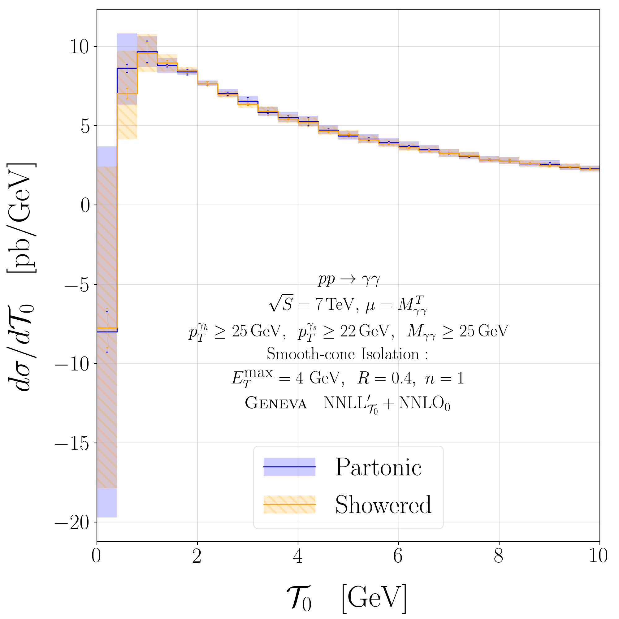
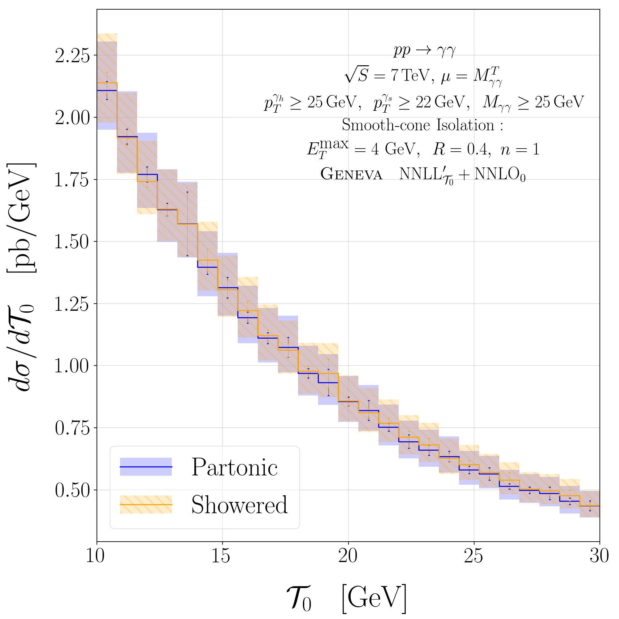
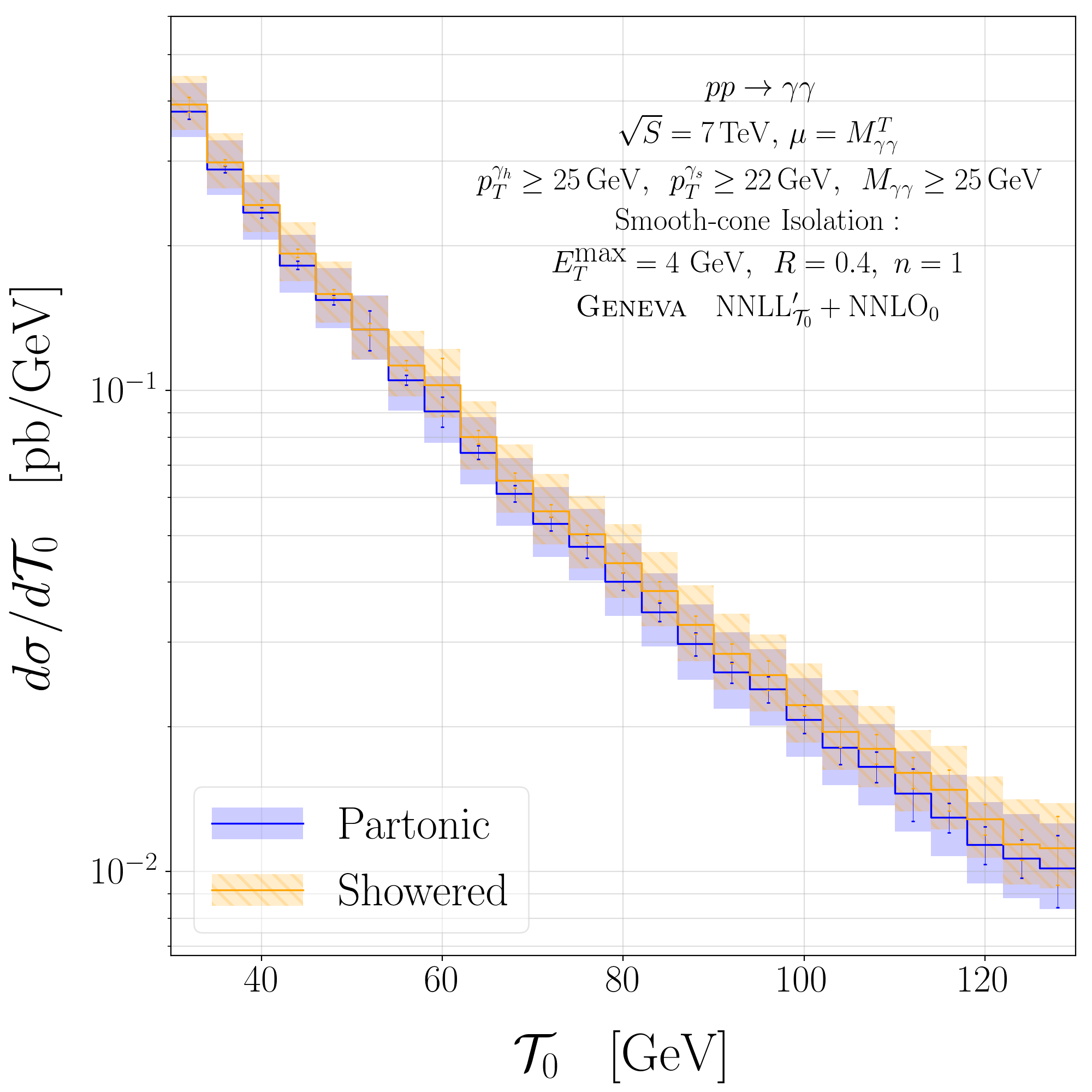
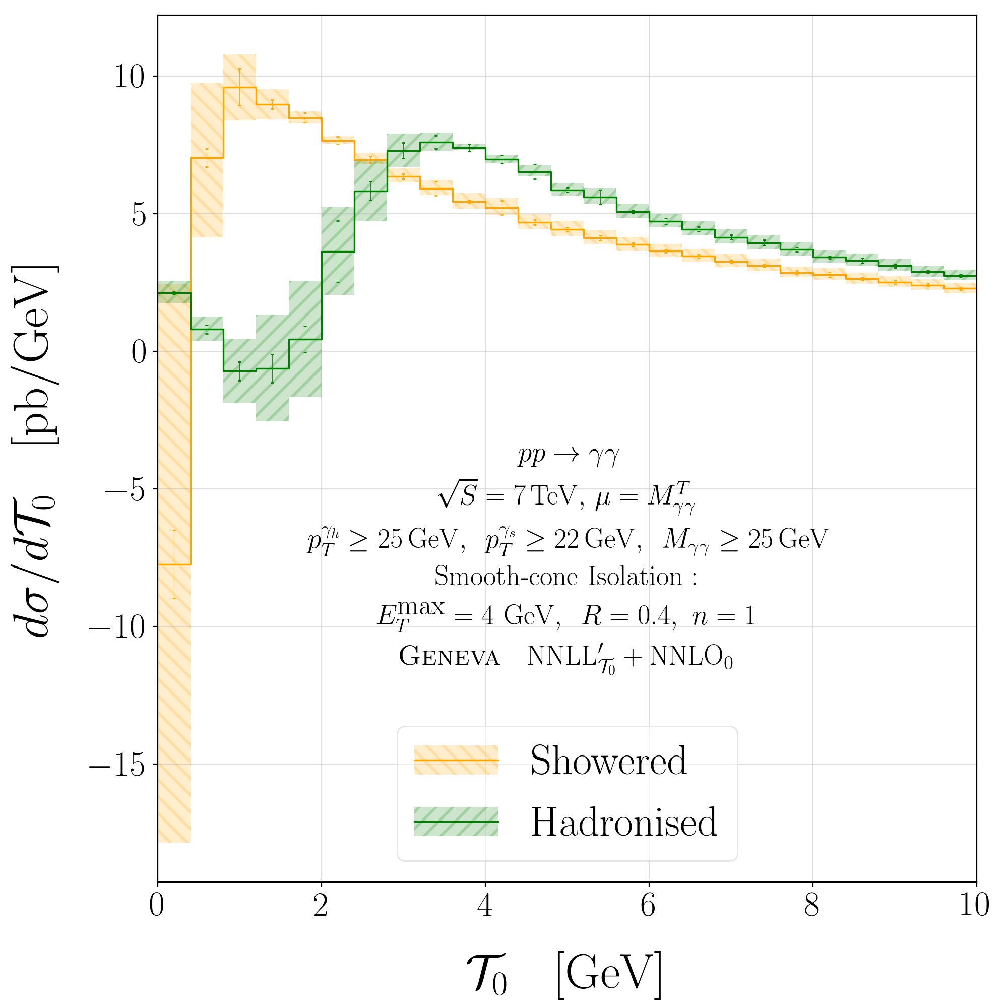
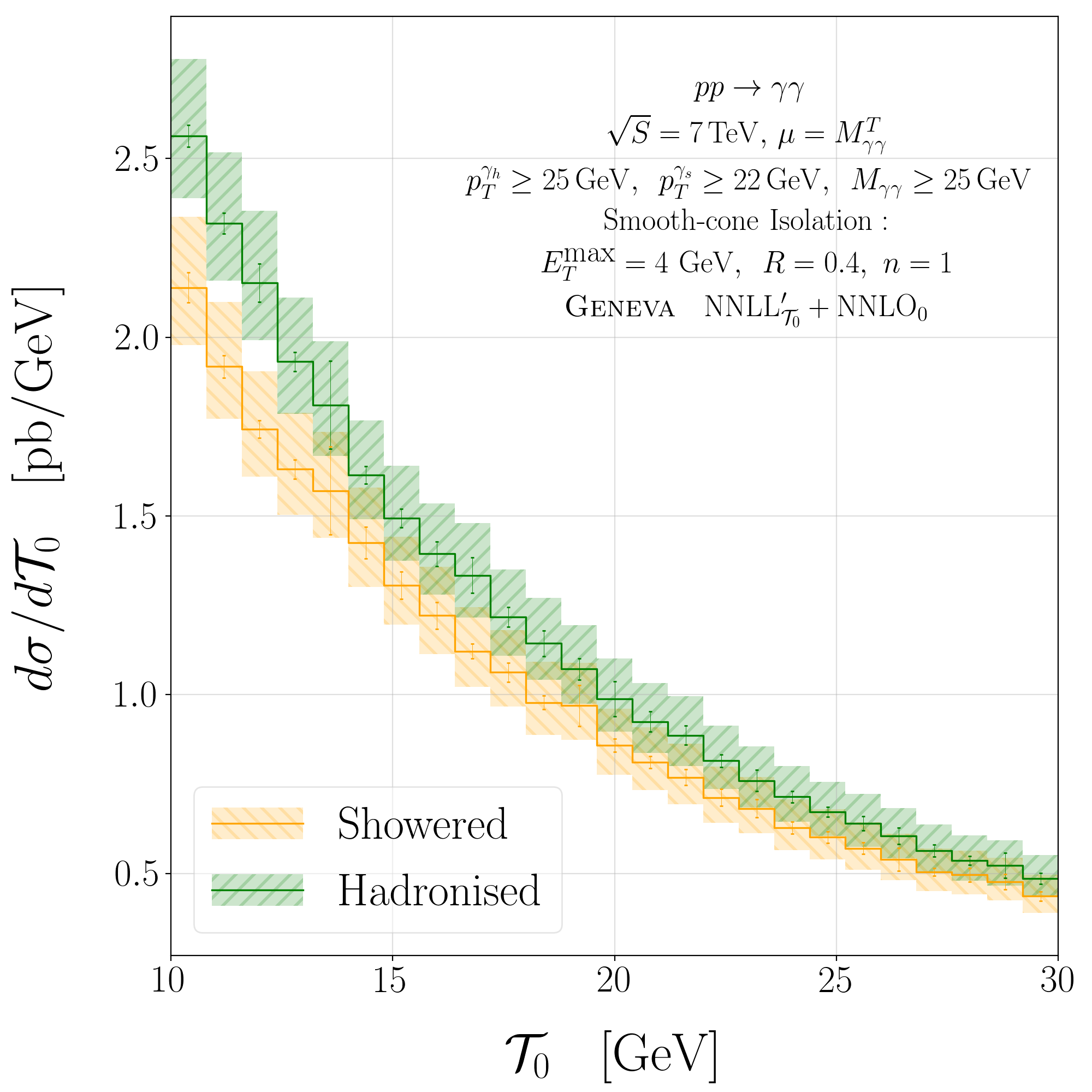
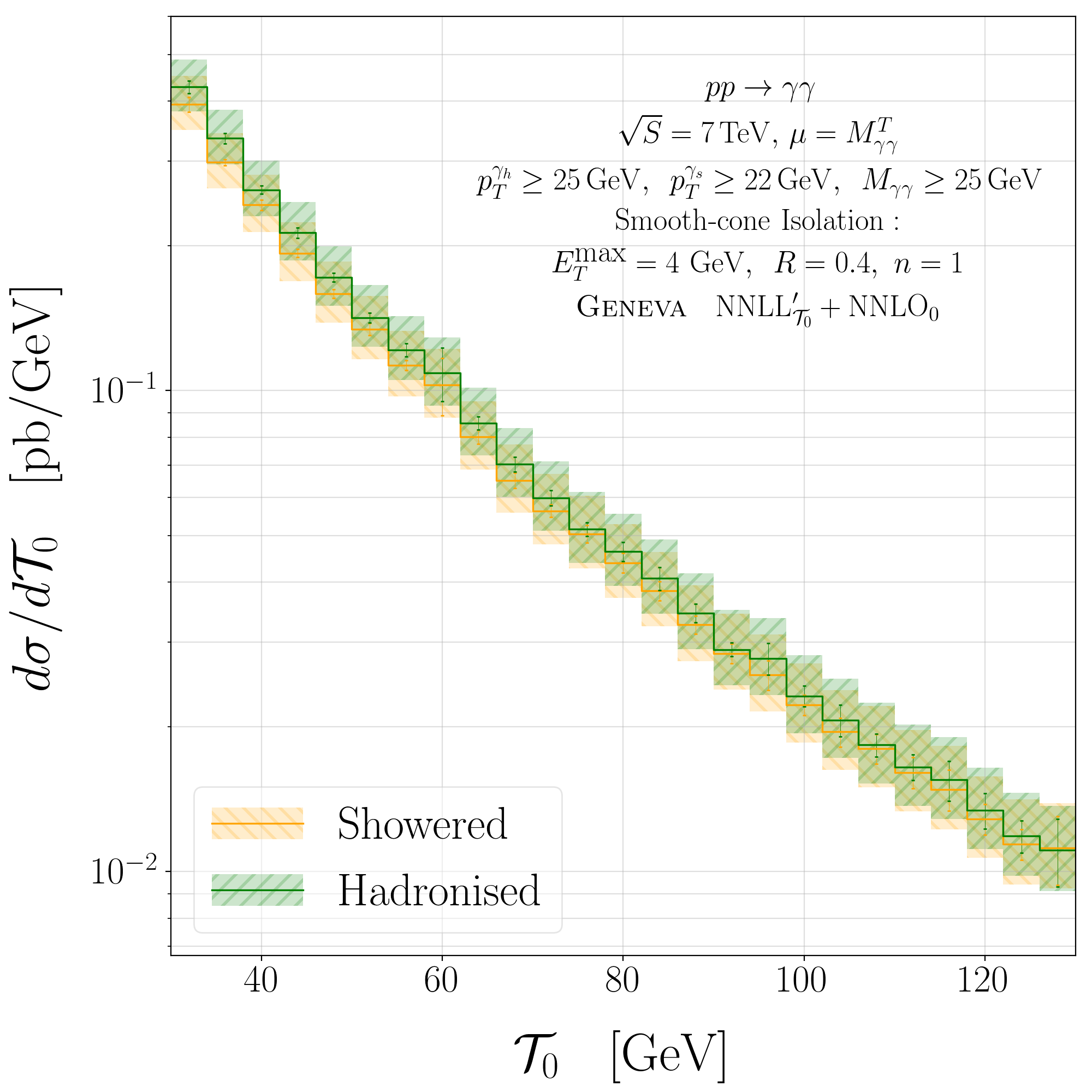
Figure 7: Comparison of $\mathcal{T}_{0}$ spectra between the partonic NNLO₀+NNLL^′ and the showered results, after interfacing to Pythia8, before the inclusion of non-perturbative effects (above). Comparison between the showered and hadronised $\mathcal{T}_{0}$ spectra (below). The peak (left), transition (centre) and tail (right) regions are shown.

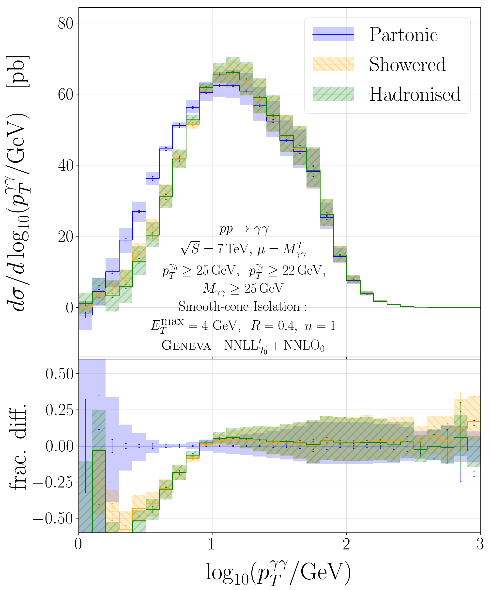
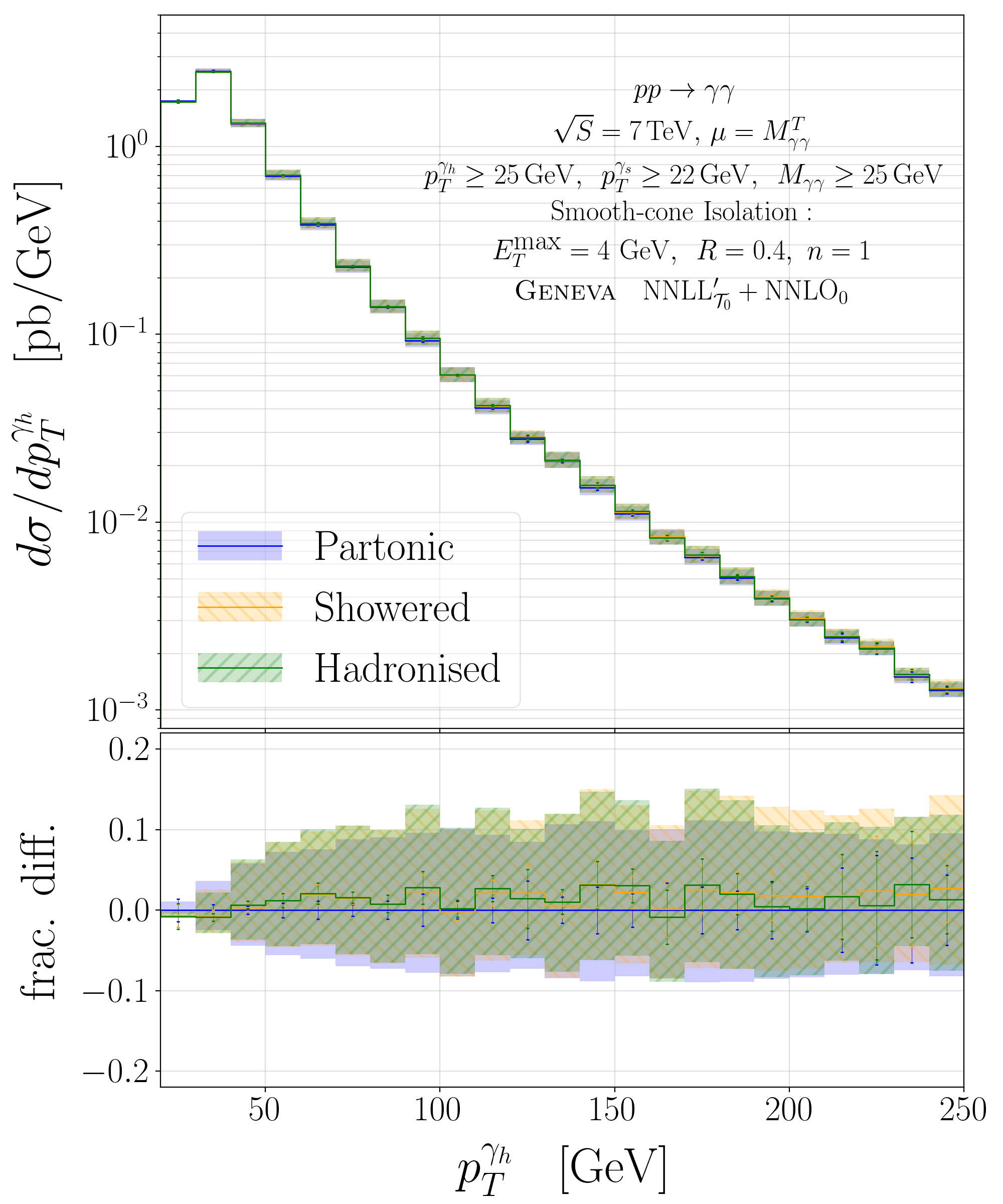
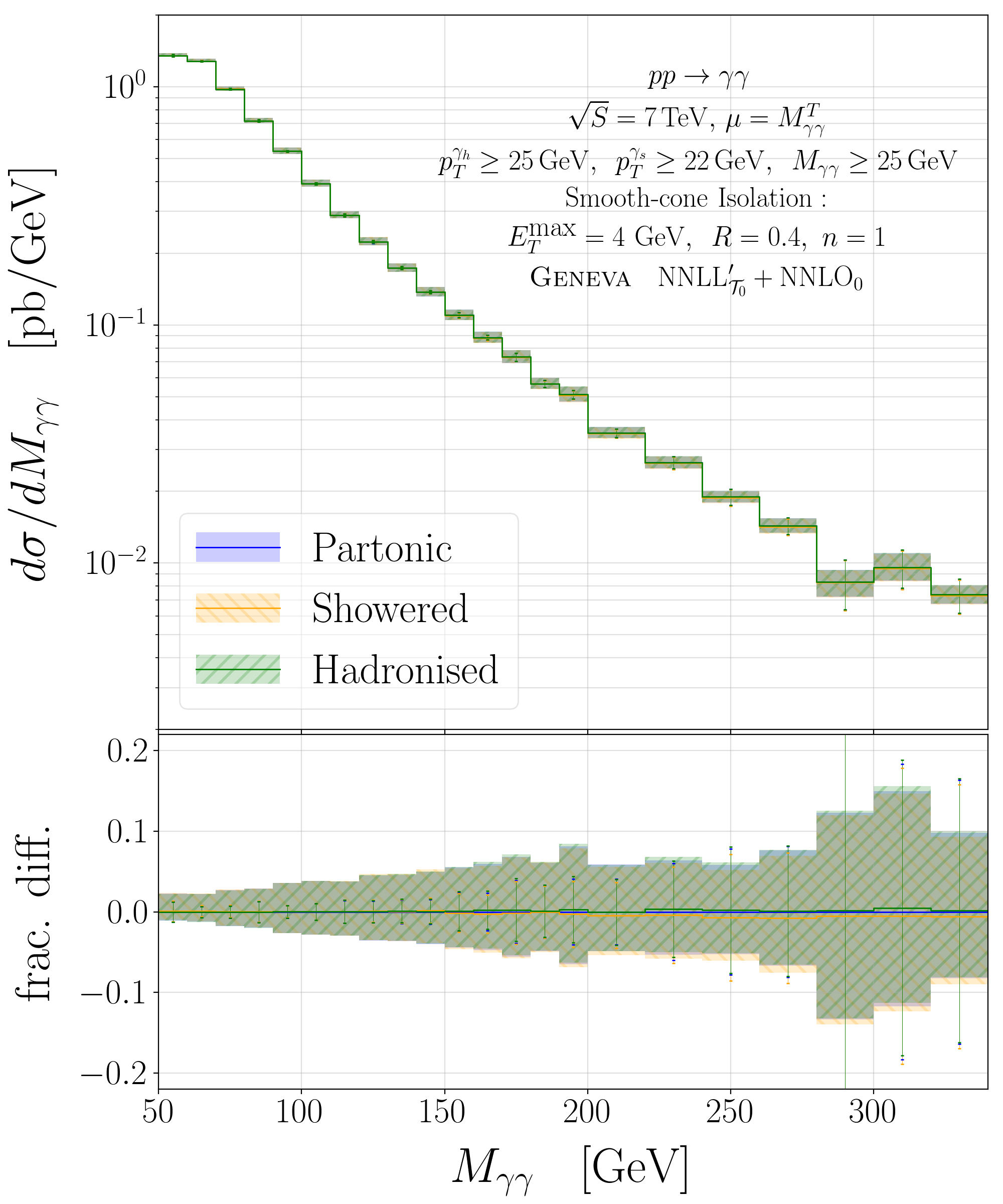
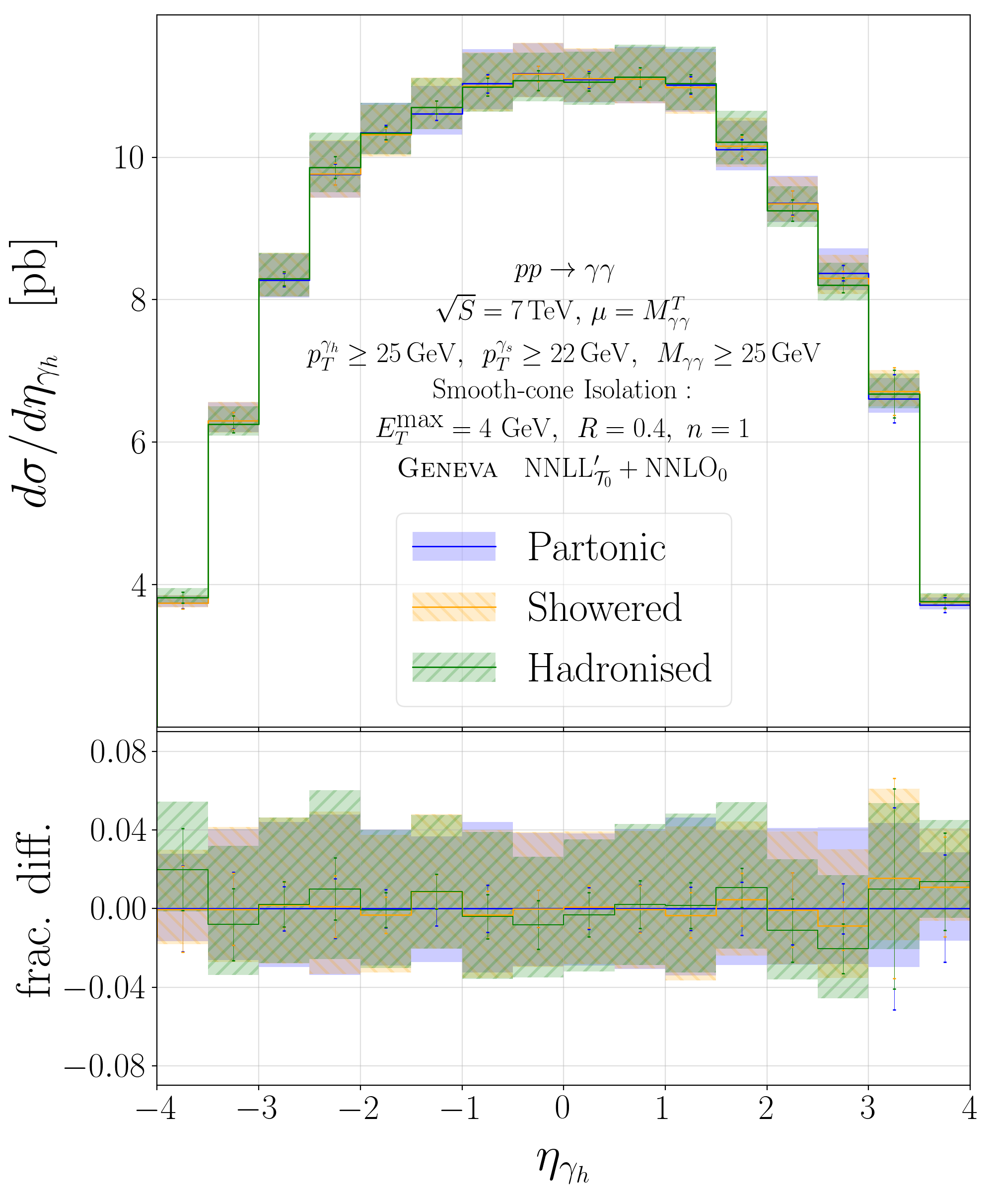
Figure 8: Comparisons of the partonic, showered and hadronised results for a selected set of distributions.

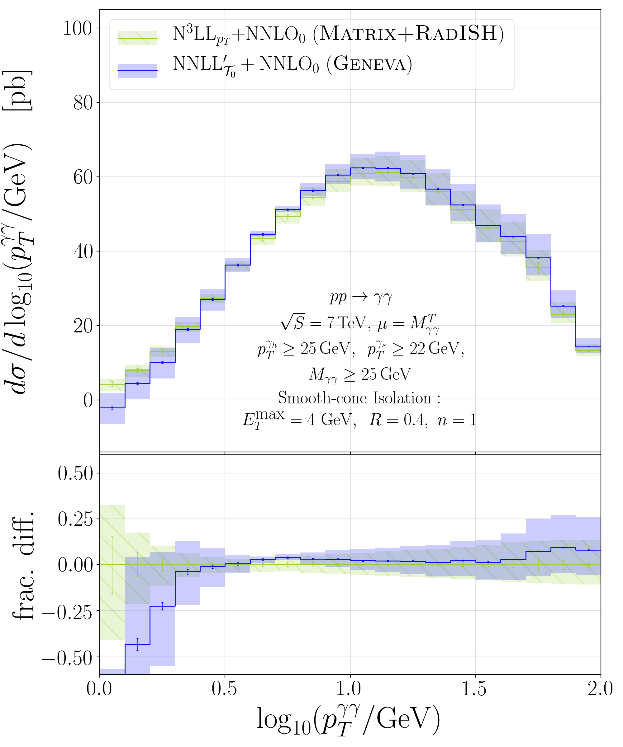
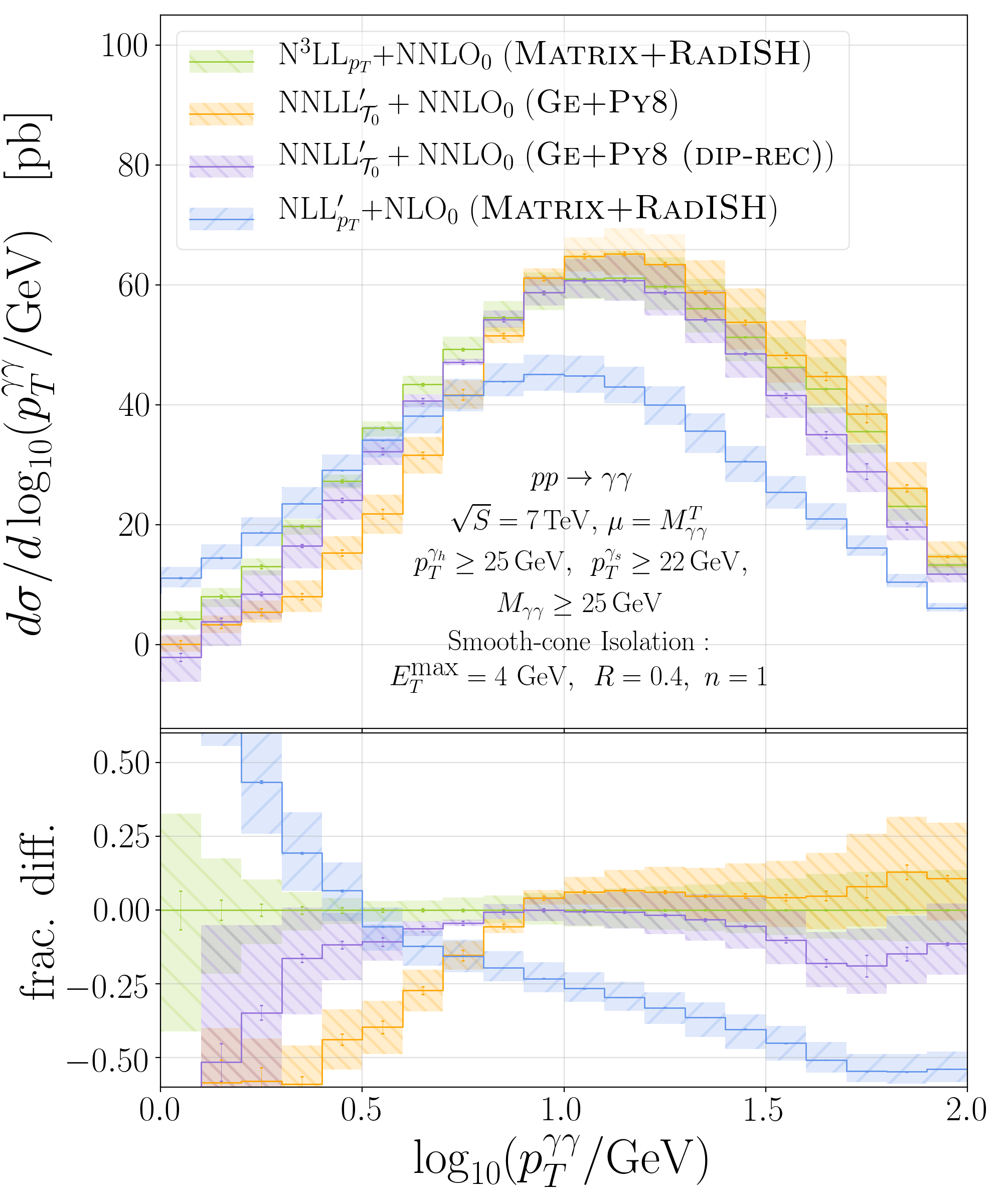
Figure 9: Comparison with Matrix+RadISH for the $p^{\gamma\gamma}_{T}$ distribution at different resummation accuracies. Geneva results before showering are shown on the left panel, after showering but before hadronisation on the right panel.

We present in the upper panel of Fig. 7 the comparison between the partonic and showered results for the $\mathcal{T}_{0}$ distribution, showing that the $\mathcal{T}_{0}$ distribution is not modified by the shower above $\mathcal{T}_{0}^{\mathrm{cut}}$. Below $\mathcal{T}^{\mathrm{cut}}_{0}$, instead, the shape of the $\mathcal{T}_{0}$ distribution is determined entirely by the shower; the effects are hardly visible since the cutoff is set to a very small value ($\mathcal{T}^{\mathrm{cut}}_{0}=10^{-2}$ GeV).

We study the impact of hadronisation, which provides the nonperturbative effects, by comparing, in the bottom panel of Fig. 7, the showered and hadronised $\mathcal{T}_{0}$ distributions. As expected, we notice a large difference between the two results only in the peak region, since the $\mathcal{T}_{0}$ observable is very sensitive to additional low-energy hadronic emissions. At larger values of $\mathcal{T}_{0}$ these corrections are instead suppressed as $\mathcal{O}(\Lambda_{\mathrm{QCD}}/Q)$ and their effects are lessened.

We further study effects due to the parton shower and hadronisation in Fig. 8, where we compare the partonic, showered and hadronised results for the transverse momentum of the photon pair, the transverse momentum of the hardest photon, the invariant mass of the photon pair and the pseudorapidity of the hardest photon. We first observe that for all the inclusive distributions, the NNLO accuracy is maintained at a very precise numerical level after both the showering and the hadronisation processes.

Moreover, although the transverse momentum of the photon pair, or any other exclusive observable, formally have the same logarithmic accuracy as the shower, we expect that it could also benefit from the high resummation accuracy of the $\mathcal{T}_{0}$ distribution. We observe that the distribution is significantly modified after the shower only in the region below $10$ GeV, while for larger values of $p^{\gamma\gamma}_{T}$, the higher-order partonic result is practically recovered. In order to quantify the quality of our predictions for this observable we can compare with the direct resummation of $p^{\gamma\gamma}_{T}$, which is performed in the Matrix+RadISH interface Kallweit:2020gva up to N³LL${}_{p_{\mathrm{T}}}$+NNLO₀ accuracy.

In the left panel of Fig. 9 we show such a comparison at the partonic level, i.e. before the shower, observing a very good agreement.  In the right panel of the same figure, we compare our results after showering but before hadronisation against the Matrix+RadISH results at both N³LL${}_{p_{\mathrm{T}}}$+NNLO₀ and NLL${}^{\prime}_{p_{\mathrm{T}}}$+NLO₀ accuracy. We include results with two different schemes for the shower recoil: the default shower recoil of Pythia8 and a second more local scheme in which the spectator parton absorbs the recoil of the initial-final dipole, preserving the transverse momentum of colourless particles. This second recoil scheme is labeled DIP-REC in the figures. Even after adding the shower effects, in particular when using the new recoil scheme, the Geneva results are in better agreement with those with higher logarithmic accuracy.

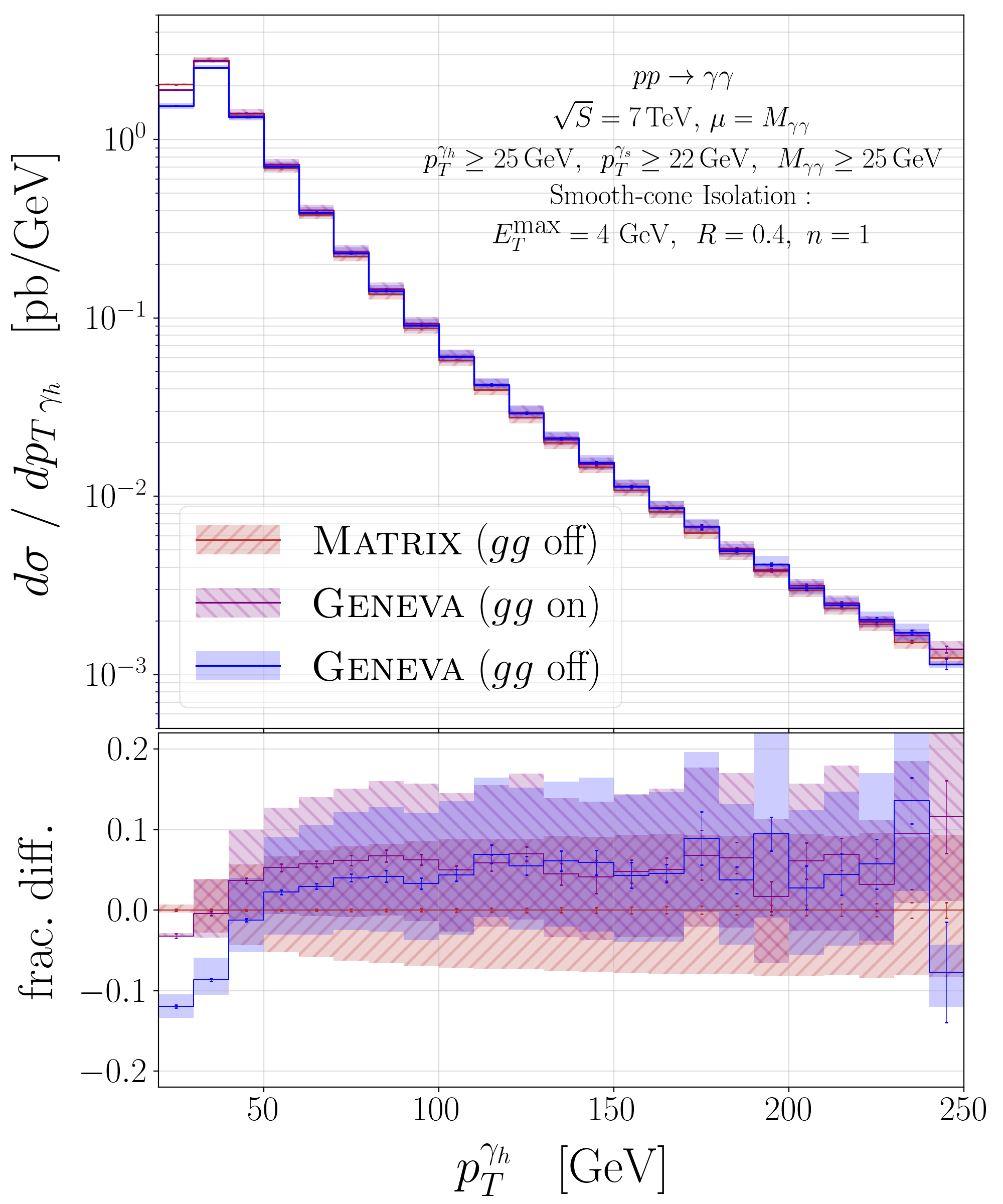
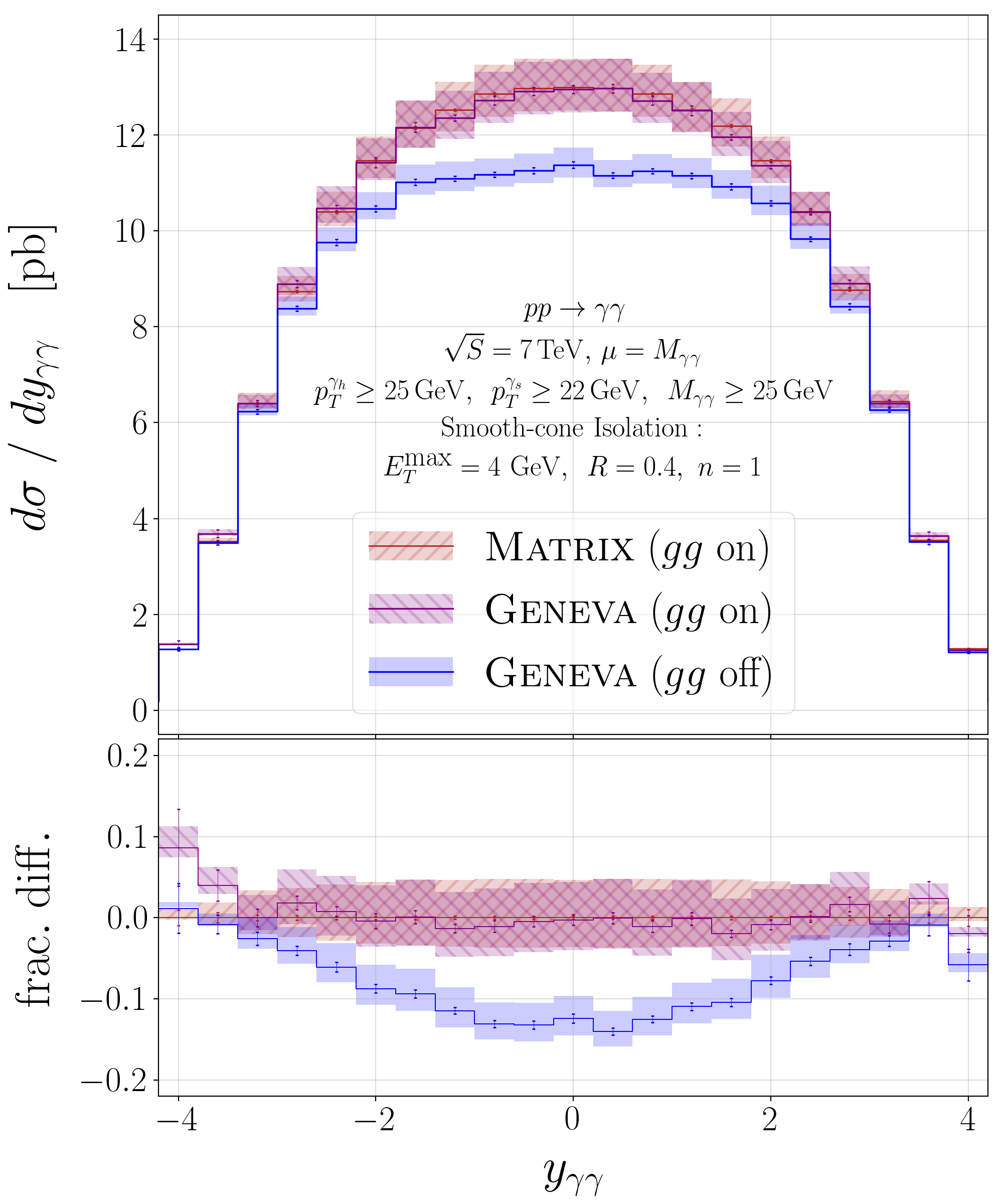
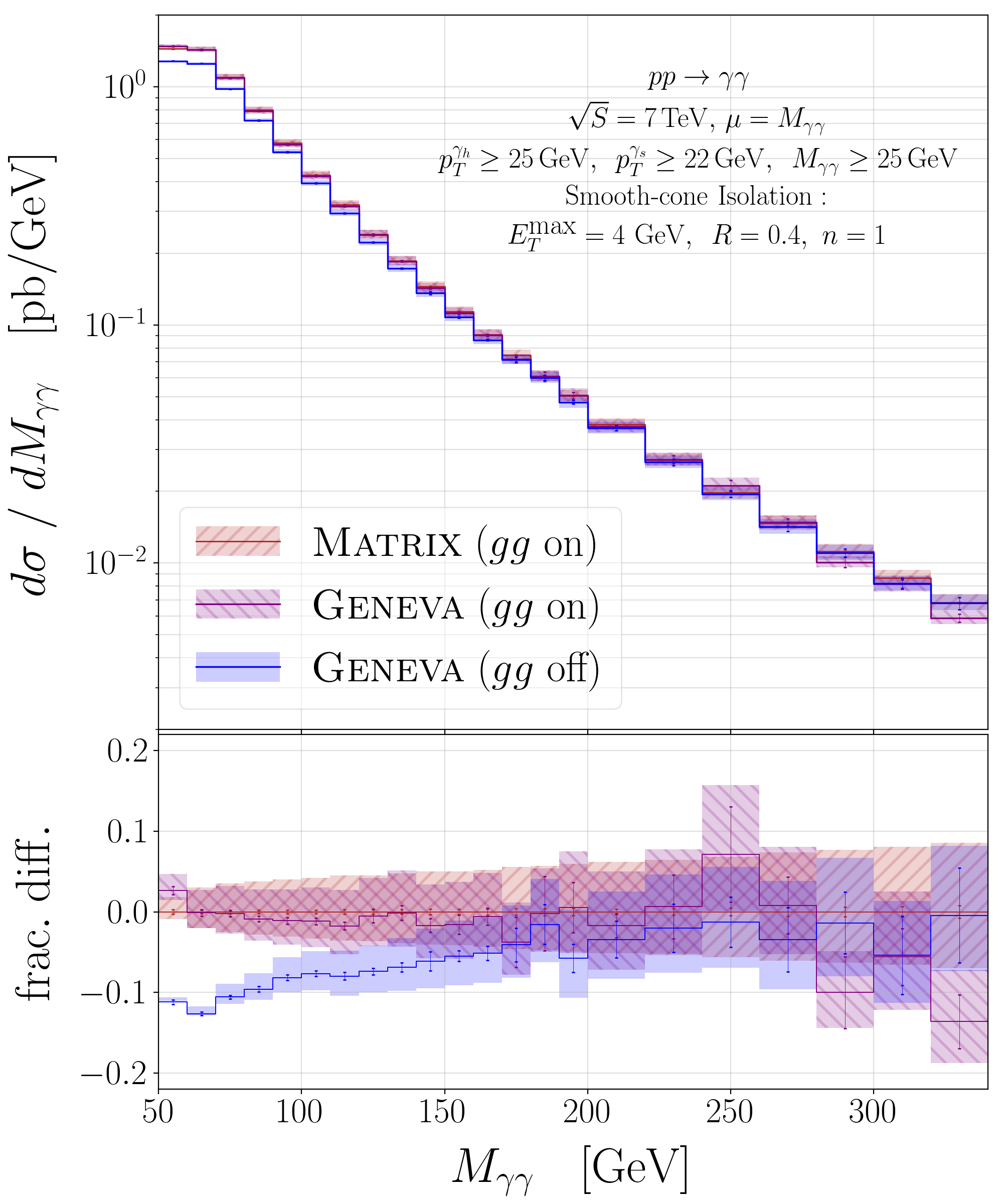
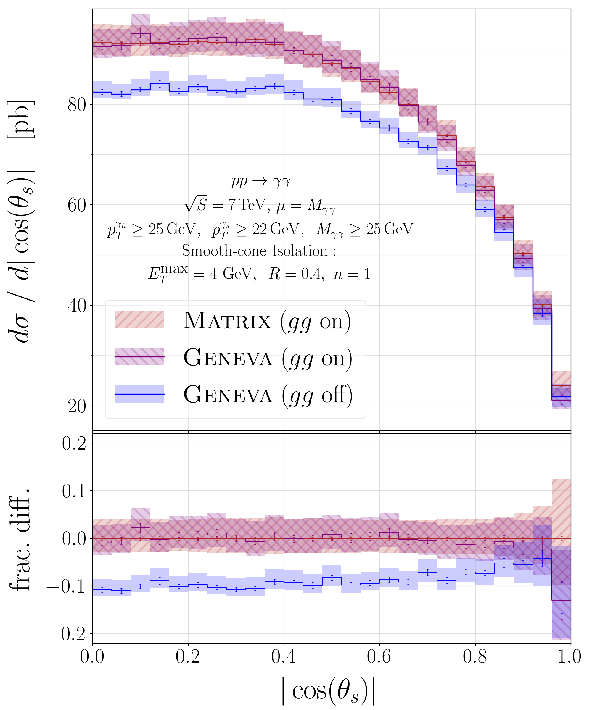
Figure 10: Comparisons between Geneva and Matrix after the inclusion of the $gg$ channel contribution. We also show the Geneva results before the inclusion of the $gg$ channel.

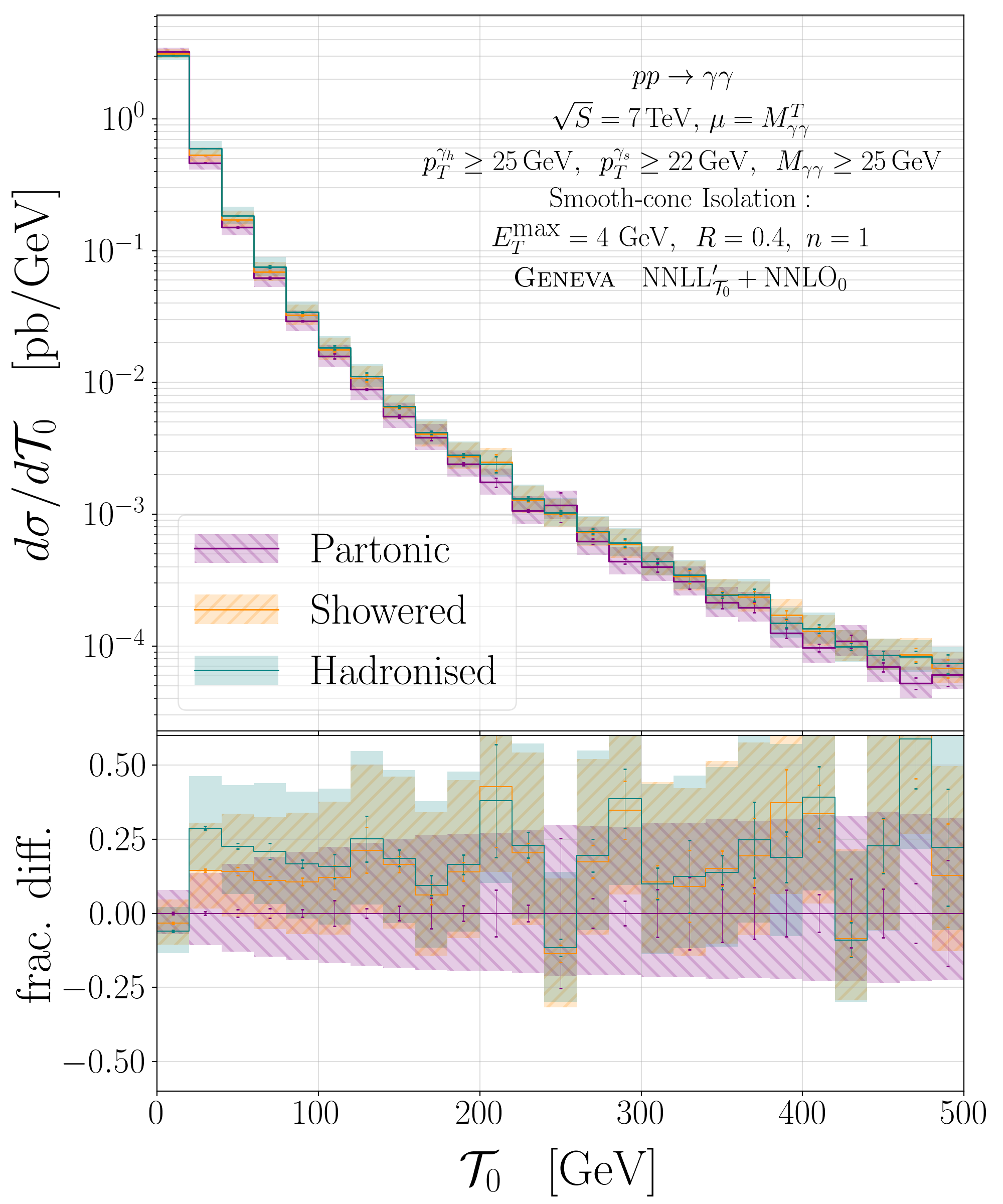
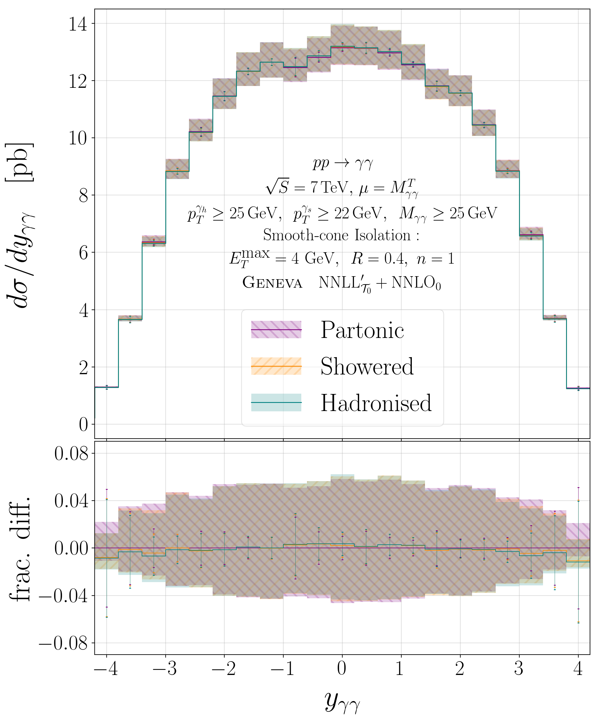
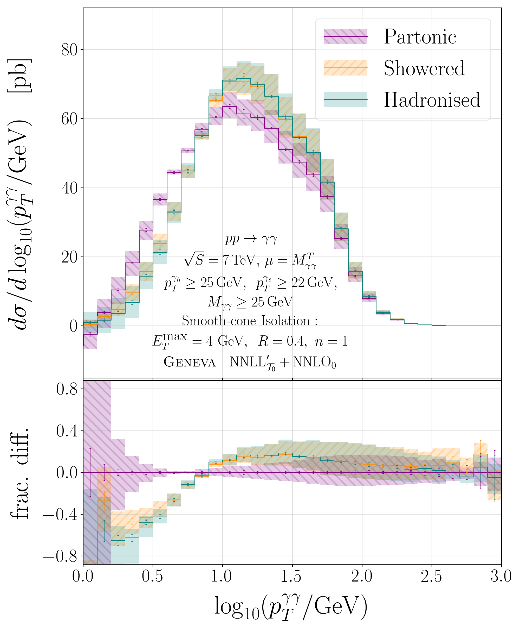
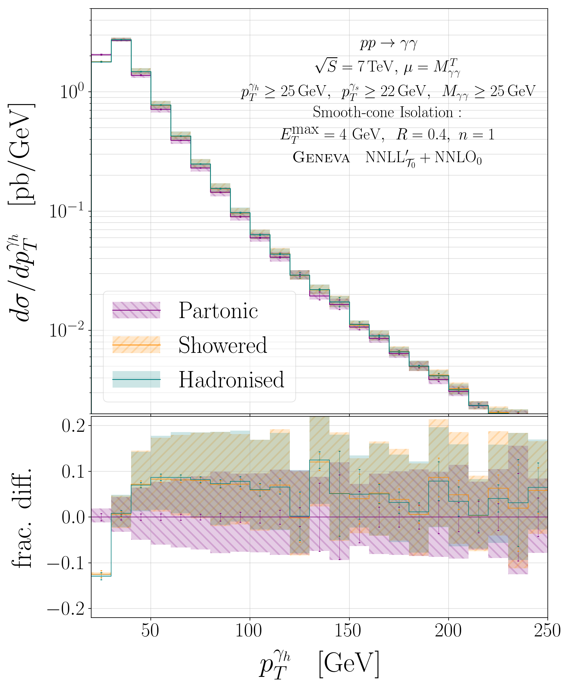
Figure 11: Comparison between the partonic, showered and hadronised spectra after the inclusion of the $gg$ channel contribution.

4.8 Inclusion of the $gg$ channel contribution

The effects of including the $gg$ channel contribution are quite large both for the total cross section (in the $6$–$10\%$ range) and the differential distributions. This is a consequence of the relative size of the gluon parton distributions at the LHC.

In Fig. 10 we compare the results of Geneva with Matrix after the inclusion of the $gg$ channel contribution for the same set of inclusive distributions presented in Fig. 6. As shown in the plots, we find very good agreement between the two calculations. We also show the effect of including the $gg$ channel contributions by comparing to the Geneva results before its inclusion. Due to the numerical relevance of this channel, its NLO QCD corrections have been the subject of dedicated studies Bern:2002jx ; Maltoni:2018zvp . However, since these terms are formally of higher order (N³LO) with respect to the $q\bar{q}$ channel contribution, we neglect them in our calculation.

When showering events in the gluon fusion channel, we set the starting scale of the shower to be equal to the highest scale present in the process, which is the partonic centre-of-mass energy. The reason for doing so is that we do not presently resum these contributions, whose resummation accuracy is then entirely given by the shower. A dedicated higher-accuracy resummation of this channel is of course possible but is left to future investigation.

In Fig. 11 we show the comparison between the partonic, showered and hadronised results after the inclusion of this channel for the $\mathcal{T}_{0}$ distribution, the rapidity of the diphoton system, the transverse momentum of the photon pair and the transverse momentum of the hardest photon. We observe somewhat larger effects after the inclusion of the shower compared to the case of the $q\bar{q}$ channel alone, especially for the $\mathcal{T}_{0}$, $p^{\gamma\gamma}_{T}$ and $p^{\gamma_{h}}_{T}$ distributions. The $y_{\gamma\gamma}$ distribution is instead left untouched by the shower. These are most likely due to the high scale at which we start the showering process. A similar behaviour was also observed for the $VH$ production process in Geneva after including the $gg$ channel contribution, as well as in the Powheg and MC@NLO implementations of similar processes Alioli:2016xab ; Heinrich:2017kxx .

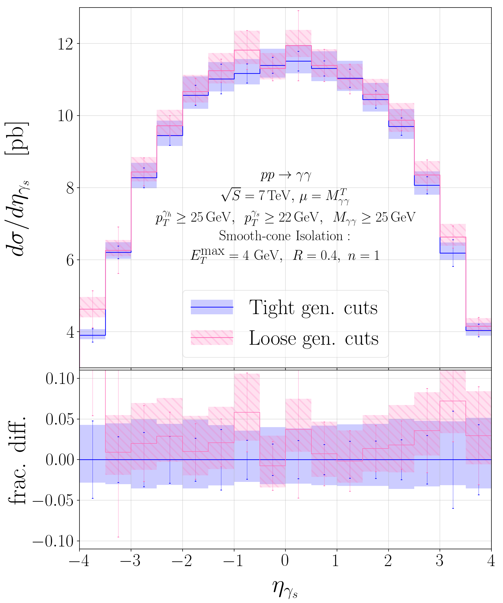
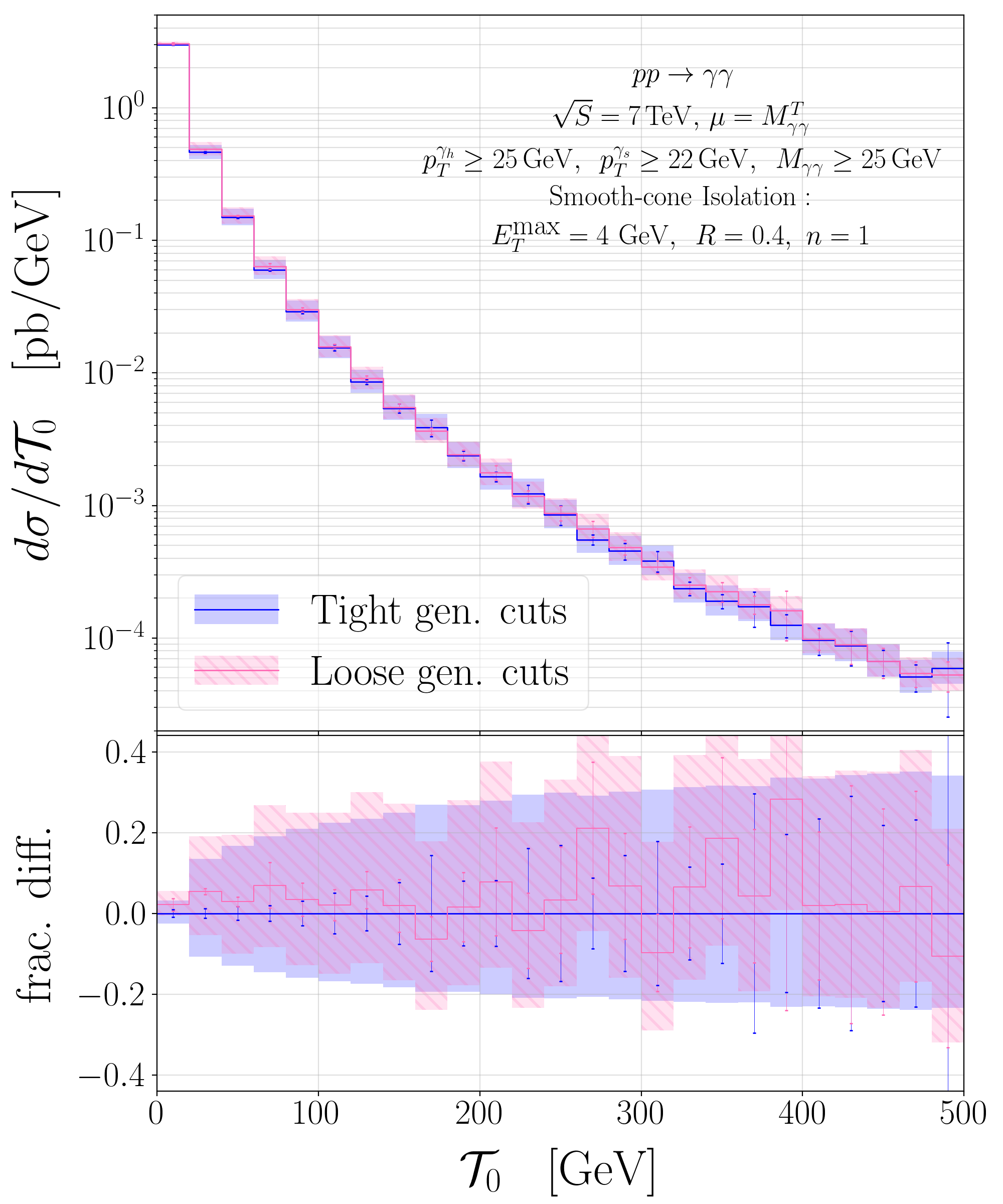
Figure 12: Comparison between two different sets of generation cuts (see text for additional details) for the pseudorapidity of the softer photon (left) and the $\mathcal{T}_{0}$ distribution (right).

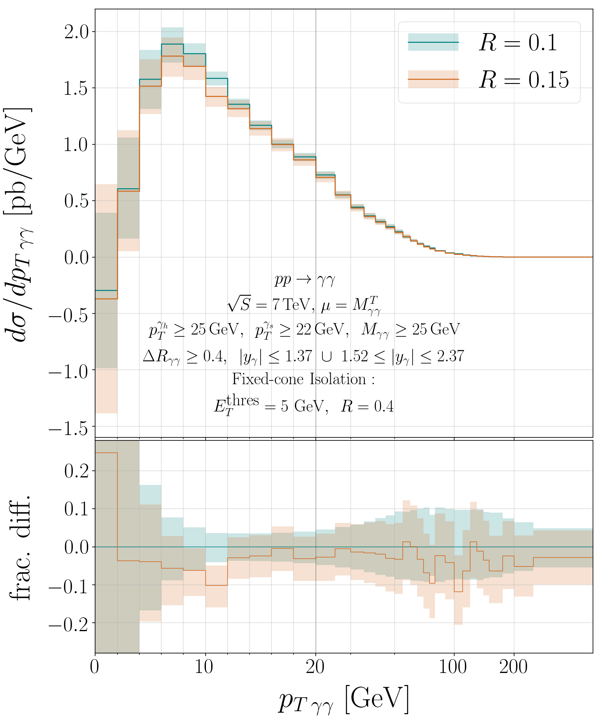
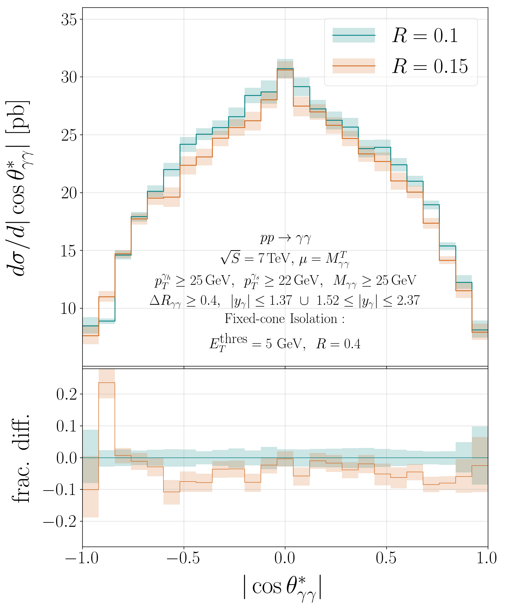
Figure 13: Comparison between Geneva + Pythia8 results after applying two different generation cuts and the same analysis cuts. The theoretical predictions have been produced by applying the Rivet analysis ATLAS_2012_I1199269 to the hadronised events. We show the transverse momentum of the photon pair (left) and the cosine of the photon angle in the Collins–Soper frame (right).

4.9 Event generation and analysis cuts

In this subsection we study the effects of applying process-defining and isolation cuts at the generation and analysis levels, both before and after shower and hadronisation. At the generation level, we are forced to use a smooth-cone isolation procedure in order to generate well-defined, IR-finite events, without fragmentation contributions. At the analysis level, however, when one is interested in comparing with data, a fixed-cone isolation algorithm is needed. For these reasons, in sec. 5 we will apply a hybrid isolation procedure, i.e. first imposing a very loose smooth-cone isolation cut at the generation level followed by a tighter fixed-cone isolation at the analysis level.

In order to check the consistency of this approach, we must first quantify the dependence of the results at the various levels of the analysis from the cuts imposed at generation. We separate this investigation into two parts: in the first, at parton level, we examine the power-suppressed isolation effects due to the phase-space projections below the jet resolution cutoffs; in the second, after the shower, we study the effect of the random momenta reshuffling due to recoil and hadronisation.

For the first part, we use the set of “tight” cuts introduced in eqs. (11) and (12), which we report here for convenience

$$p^{\gamma_{h}}_{T}\geq 25\,\,\mathrm{GeV},\quad p^{\gamma_{s}}_{T} \geq 22\,\,\mathrm{GeV},\quad M_{\gamma\gamma}\geq 25\,\,\mathrm{GeV}\,,$$

$$E^{\mathrm{max}}_{T}=4\,\,\mathrm{GeV},\quad R_{\mathrm{iso}}=0.4,\quad\mathrm{and}\quad n=1\,,$$ (53)

and the second set of “loose” cuts given by

$$p^{\gamma_{h}}_{T}\geq 18\,\,\mathrm{GeV},\quad p^{\gamma_{s}}_{T} \geq 15\,\,\mathrm{GeV},\quad M_{\gamma\gamma}\geq 25\,\,\mathrm{GeV}\,,$$

$$E^{\mathrm{max}}_{T}=4\,\,\mathrm{GeV},\quad R_{\mathrm{iso}}=0.1,\quad\mathrm{and}\quad n=1\,.$$ (54)

We first generate the events by applying the set of loose cuts in eq. (4.9) and, as a second step, we analyse them by applying the tighter cuts of eq. (4.9) before showering. We compare these predictions to the results obtained by directly applying the set of tight cuts at generation level.

This is shown in Fig. 12 for the pseudorapidity of the softer photon and the $\mathcal{T}_{0}$ distribution, where we show the results of the calculation directly carried out with tight generation cuts together with that where we apply loose generation cuts (as in eq. (4.9)) and tighter cuts at the analysis level. The two predictions are in good agreement and this gives us confidence that our results are not strongly dependent on the generation cuts applied.

For the second part, one should expect that power-suppressed effects connected with the recoil after any emission could modify the momenta of the final-state particles and, consequently, result in a different rate of events passing the analysis cuts compared to those passing the generation cuts. This effect is particularly severe after the shower, since multiple emissions can greatly reshuffle the final-state momenta. The same applies to the reshuffle used by SMC programs to impose momentum conservation after hadronisation.

In order to quantify these effects we compare in Fig. 13 results obtained employing the loose generation cuts in eq. (4.9) with the values $R_{\textrm{iso}}=0.1$ and $R_{\textrm{iso}}=0.15$ and applying the ATLAS analysis cuts which are introduced later in eqs. (56) and (57) of sec. 5. The figure shows reasonable agreement between the two predictions for the transverse momentum of the photon pair and the cosine of the photon angle in the Collins–Soper frame, demonstrating that the size of these effects is not large for variations of the isolation radius at generation level. However, qualitatively we did find a stronger dependence of the final results on the choice of the generation cuts on the photons’ transverse momenta.

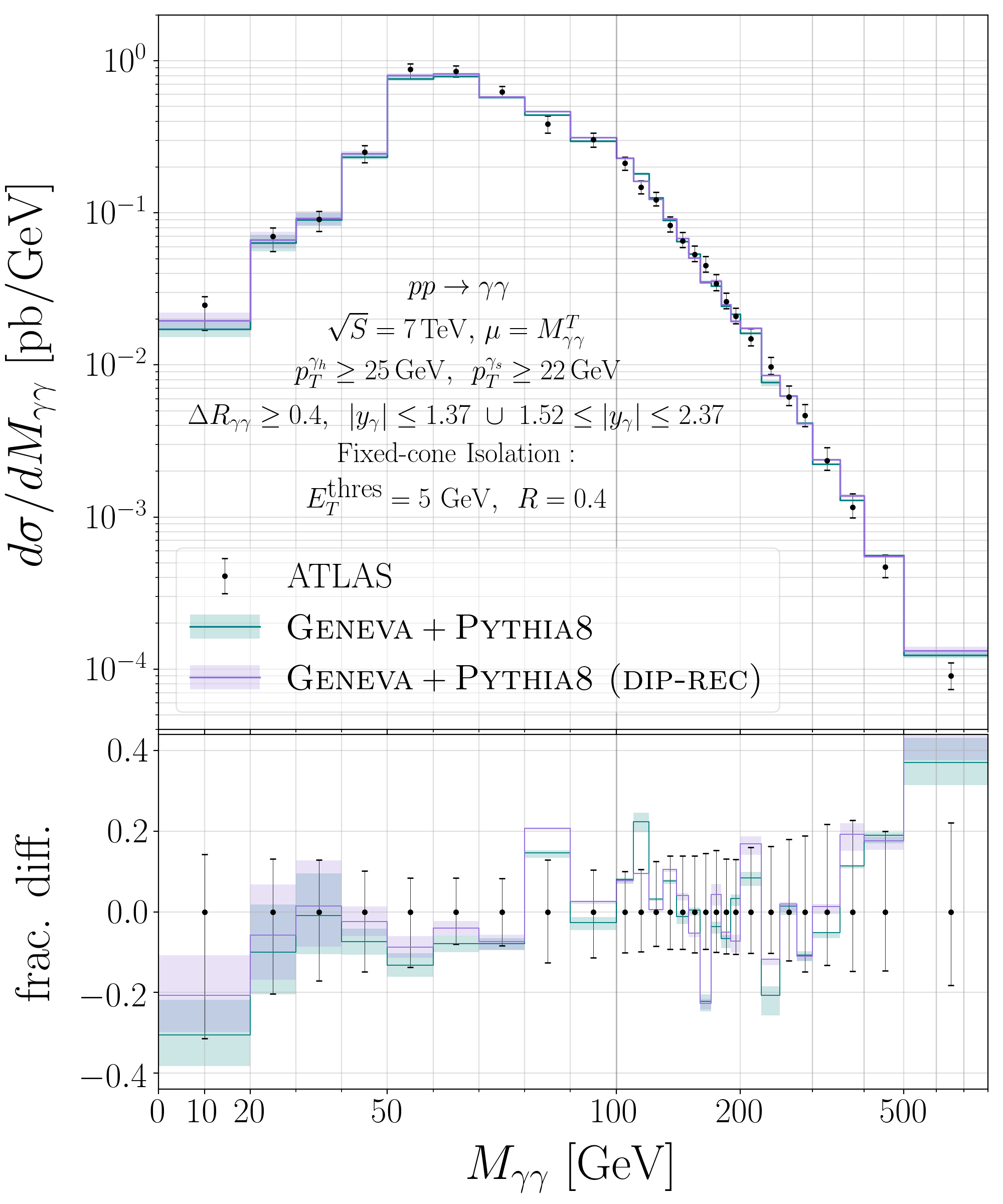
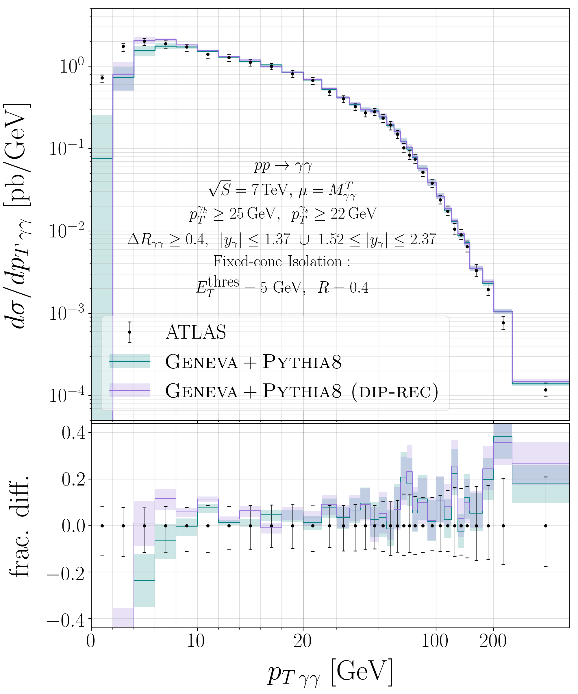
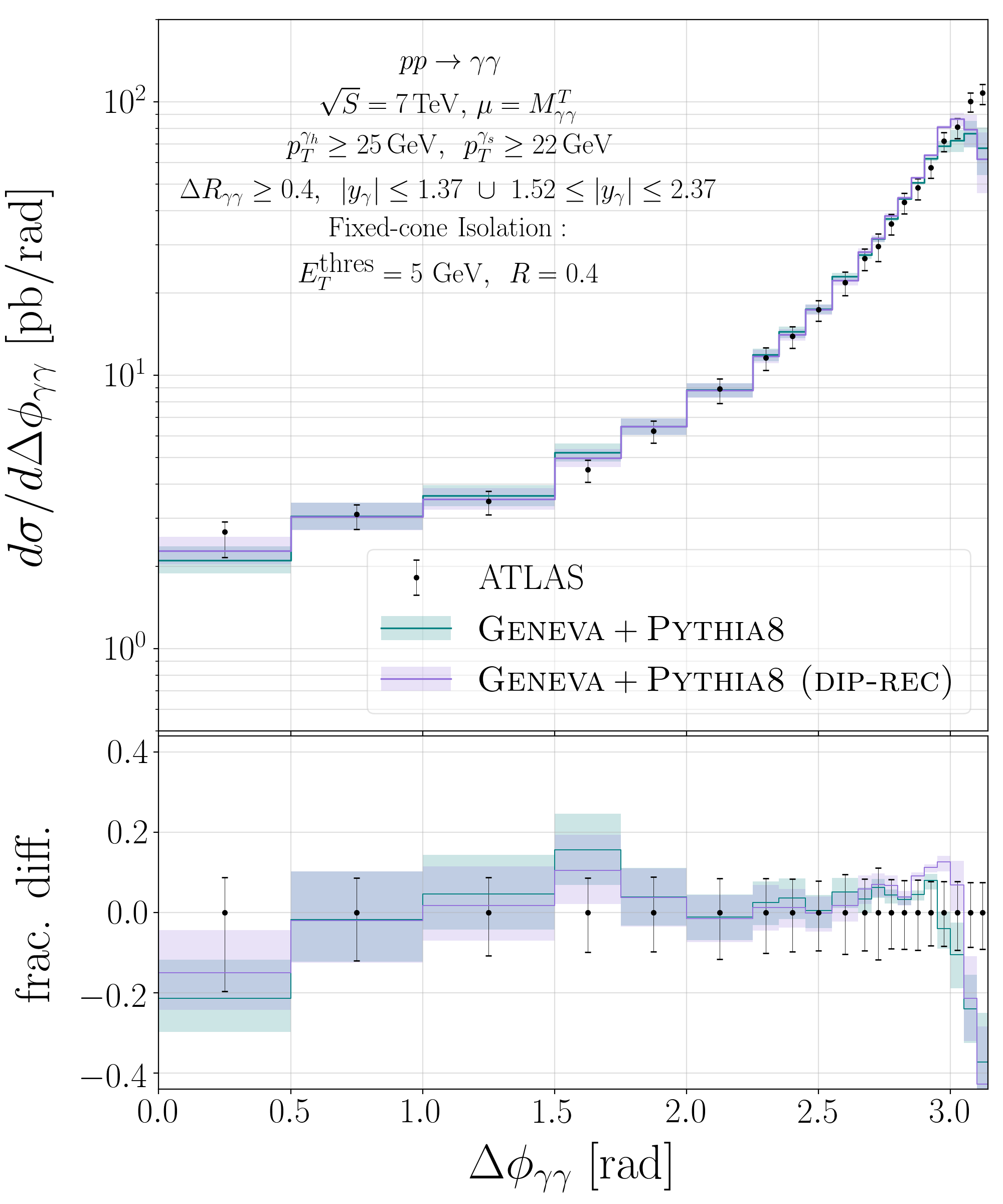
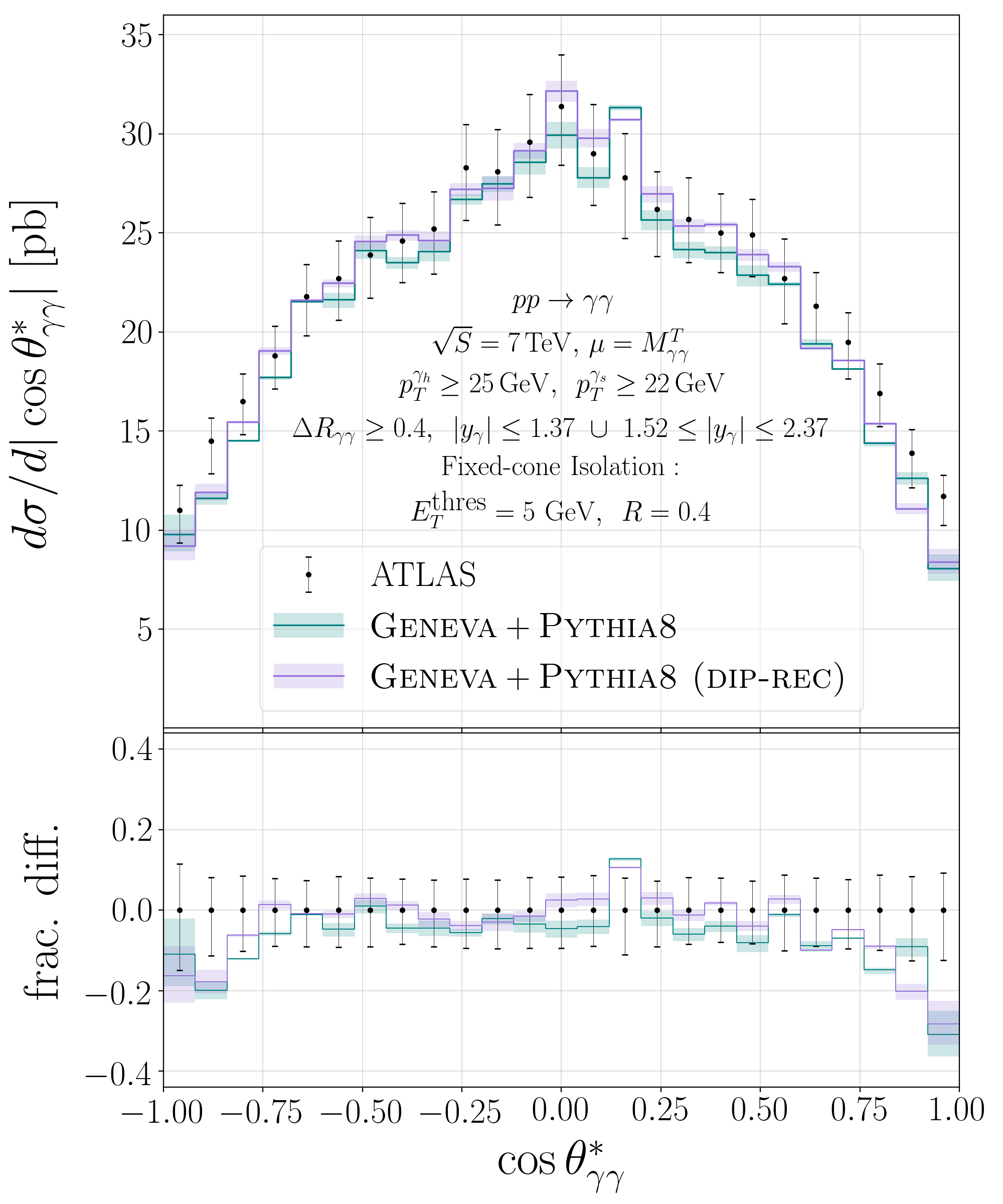
Figure 14: Comparison between Geneva + Pythia8 and the 7 TeV data from ATLAS Aad:2012tba . The theoretical predictions have been produced by applying the Rivet analysis ATLAS_2012_I1199269 to the hadronised events. We show the invariant mass of the photon pair (top left), the transverse momentum of the diphoton system (top right), the azimuthal-angle separation between the two photons (bottom left) and the cosine of the polar angle in the Collins–Soper frame of the diphoton system (bottom right).

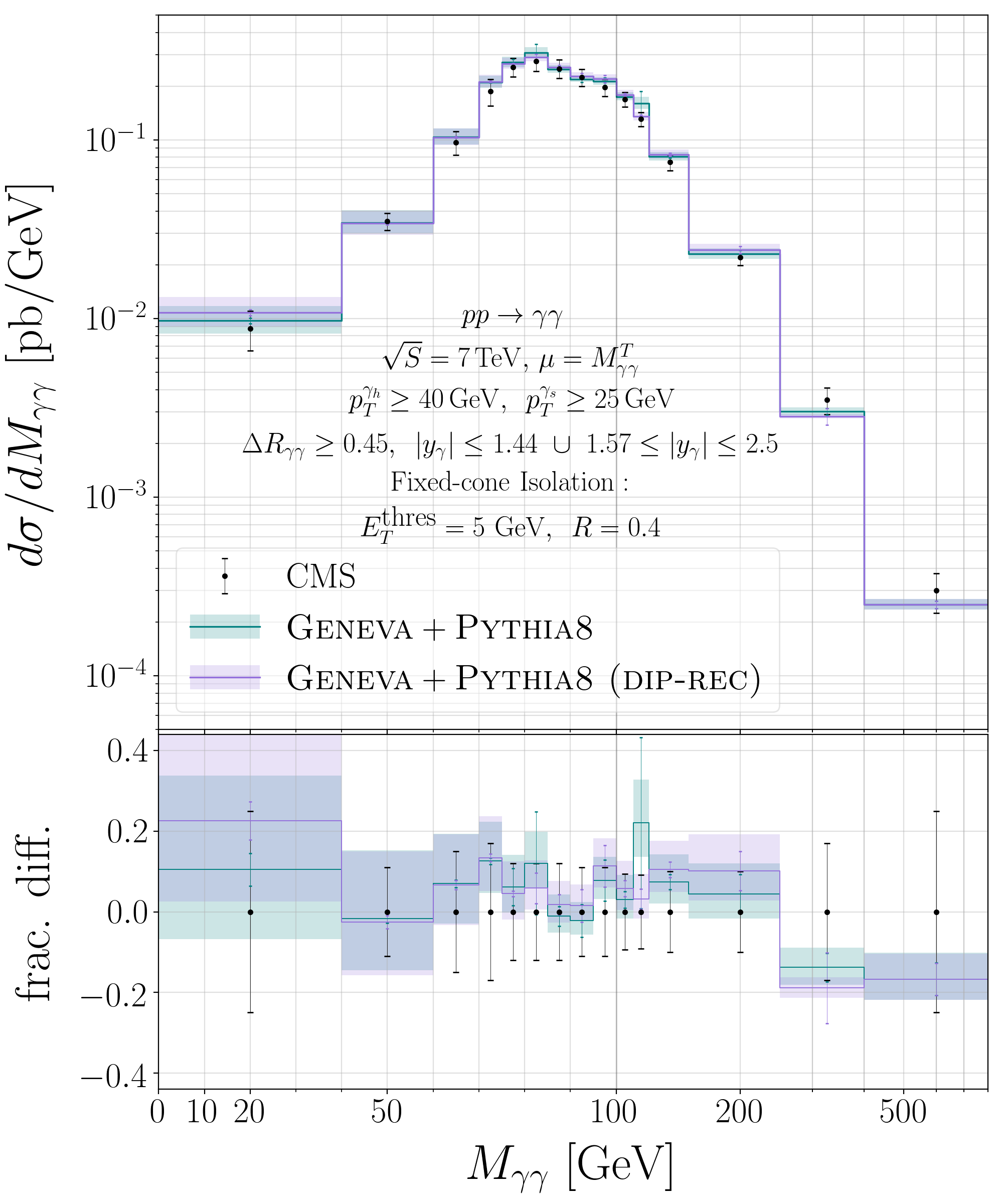
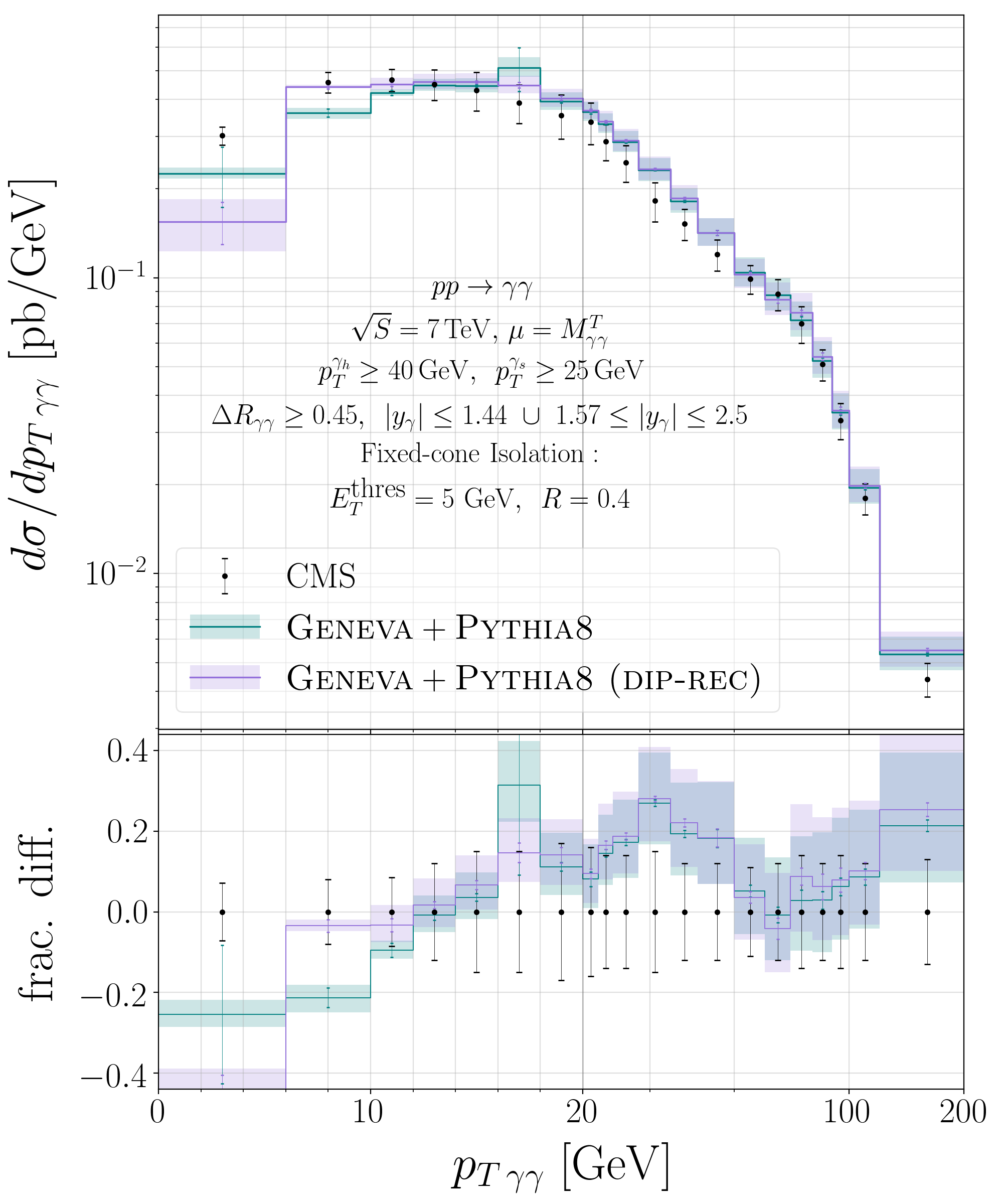
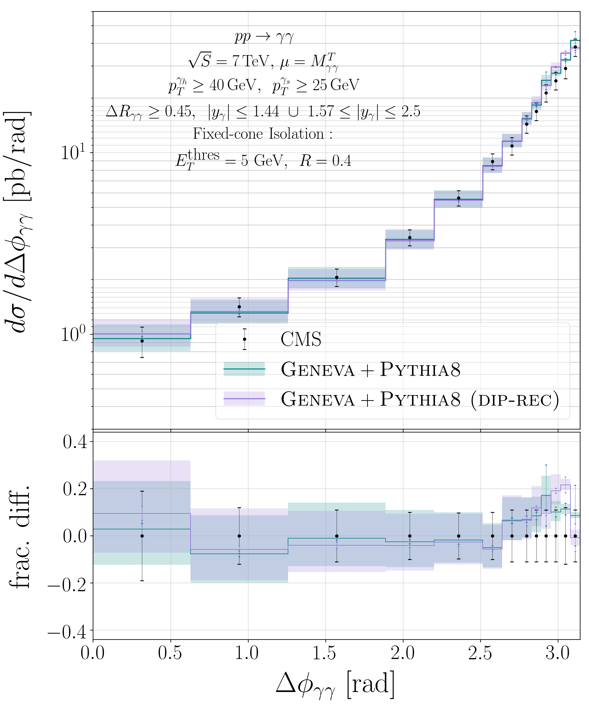
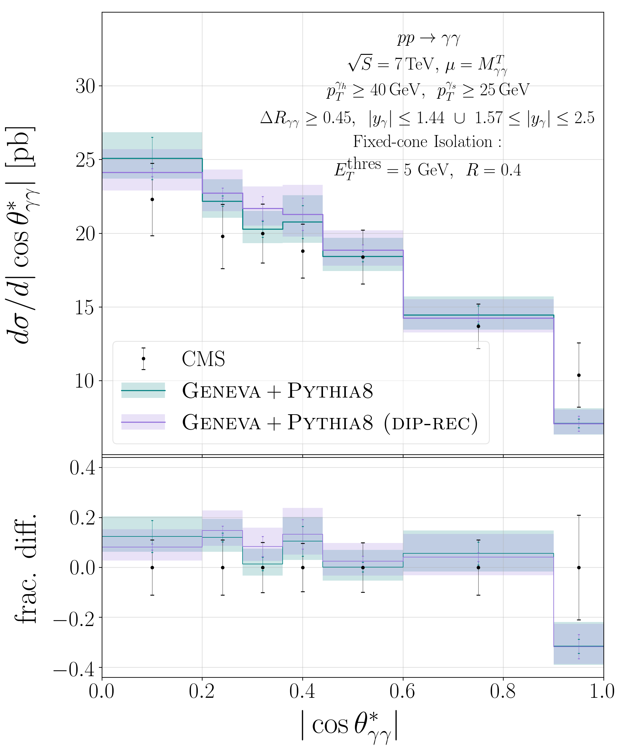
Figure 15: Comparison between Geneva + Pythia8 and the 7 TeV data from CMS Chatrchyan:2014fsa . We show invariant mass of the photon pair (top left), the transverse momentum of the diphoton system (top right), the azimuthal-angle separation between the two photons (bottom left) and the cosine of the polar angle in the Collins–Soper frame of the diphoton system (bottom right).

5 Results and comparison to LHC data

In this section we compare our predictions against $7$ TeV LHC data obtained from both ATLAS Aad:2012tba and CMS Chatrchyan:2014fsa . We employ the hybrid isolation procedure, as detailed in sec. 2 and sec. 4.9. This means that we first generate partonic events with looser smooth-cone isolation cuts, and only after the shower and hadronisation procedures do we apply the tighter analysis cuts and fixed-cone isolation algorithms which are used by the ATLAS and CMS experiments.

For these particular comparisons, we generate events using the NNPDF31_nnlo_as_0118 PDF set Ball:2017nwa . We set the FO scale to $\mu_{\mathrm{FO}}=M_{\gamma\gamma}^{T}$ and apply the following process-defining cuts at generation level:

$$p^{\gamma_{h}}_{T}\geq 18\,\,\mathrm{GeV},\quad p^{\gamma_{s}}_{T} \geq 15\,\,\mathrm{GeV},\quad M_{\gamma\gamma}\geq 1\,\,\mathrm{GeV}\,,$$

$$E^{\mathrm{max}}_{T}=4\,\,\mathrm{GeV},\quad R_{\mathrm{iso}}=0.1,\quad\mathrm{and}\quad n=1\,.$$ (55)

Note that, in principle, there is no need to require a lower limit on the invariant mass of the photon pair, but, since our hard function is evaluated at $\mu_{H}=M_{\gamma\gamma}$ in the resummation region, we set this lower cutoff so that $\alpha_{s}(\mu_{H})$ is not evaluated at scales which are too small.

We then shower and hadronise the partonic events generated with the cuts in eq. (5). To this end, we use Pythia8 and, in order to avoid any contamination by photons coming from hadronic jets, we prevent the decay of hadrons. For this comparison we also include the MPI and the QED shower effects. However, we do not allow QED splittings of photons into quarks or leptons. We obtained our predictions by using two different recoil schemes for the shower: the default shower recoil of Pythia8 and a more local dipole recoil (DIP-REC).

In Fig. 14 we show the comparison between our predictions and the ATLAS data at 7 TeV Aad:2012tba for the invariant mass of the photon pair $M_{\gamma\gamma}$, the transverse momentum of the diphoton system $p^{\gamma\gamma}_{T}$, the azimuthal-angle separation between the two photons $\Delta\phi_{\gamma\gamma}$ and the cosine of the polar angle $\theta^{*}_{\gamma\gamma}$ in the Collins–Soper frame of the diphoton system. The comparison is carried out by applying to the showered and hadronised events the Rivet Buckley:2010ar analysis ATLAS_2012_I1199269, which is provided by the ATLAS collaboration. This requires the presence of two isolated photons by means of a fixed-cone isolation criterion with parameters

$$E^{\mathrm{max}}_{T}=4\,\,\mathrm{GeV},\quad R_{\mathrm{iso}}=0.4\,,$$ (56)

and the set of cuts

$$p^{\gamma_{h}}_{T}\geq 25\,\,\mathrm{GeV},\quad p^{\gamma_{s}}_{T} \geq 22\,\,\mathrm{GeV},\quad\Delta R_{\gamma\gamma}\geq 0.4\quad\mathrm{and}\quad|y_{\gamma}|\leq 1.37\ \cup\ 1.52\leq|y_{\gamma}|\leq 2.37\,,$$ (57)

where $\Delta R_{\gamma\gamma}=\sqrt{\Delta{\eta_{\gamma\gamma}}^{2}+\Delta{\phi_{\gamma\gamma}}^{2}}$ is the separation between the photons. Overall, we observe very good agreement between the theoretical predictions and the ATLAS data. For the invariant mass distribution, in the region $M_{\gamma\gamma}\geq 350$ GeV, above the $t\bar{t}$ production threshold, the theoretical predictions seem to depart from data. Here we expect that the inclusion of EW corrections and of the two-loop diagrams with a closed top-quark loop in the hard function will improve the theoretical description. We also observe a deviation in the extreme region $\Delta\phi_{\gamma\gamma}\sim\pi$ of the $\Delta\phi_{\gamma\gamma}$ distribution.

Next, we compare against the CMS data at 7 TeV Chatrchyan:2014fsa . The CMS analysis uses a fixed-cone isolation algorithm with parameters

$$E^{\mathrm{max}}_{T}=5\,\,\mathrm{GeV},\quad R_{\mathrm{iso}}=0.4\,,$$ (58)

and the set of cuts

$$p^{\gamma_{h}}_{T}\geq 40\,\,\mathrm{GeV},\quad p^{\gamma_{s}}_{T} \geq 25\,\,\mathrm{GeV},\quad\Delta R_{\gamma\gamma}\geq 0.45\quad\mathrm{and}\quad|y_{\gamma}|\leq 1.44\ \cup\ 1.57\leq|y_{\gamma}|\leq 2.5\,.$$ (59)

The comparison between the predictions obtained with Geneva + Pythia8 and the CMS data is shown in Fig. 15 for the same set of distributions presented for the ATLAS case. Unfortunately, since no corresponding Rivet analysis is available, we have implemented the aforementioned cuts in the Geneva analyser. The $M_{\gamma\gamma}$ distribution is shown with a linear scale on the abscissa up to $100$ GeV and a logarithmic scale beyond. Similarly, the $p^{\gamma\gamma}_{T}$ distribution is shown with a linear scale up to $20$ GeV and a logarithmic scale beyond. We observe a similarly good agreement for the inclusive distributions as for ATLAS. Close to $\Delta\phi_{\gamma\gamma}\sim\pi$ the photons’ azimuthal separation shows an opposite trend compared to that of ATLAS, but our predictions in this case always agree with CMS data within experimental errors.

For both experiments, the $p_{T,\gamma\gamma}$ prediction also shows some systematic trends, undershooting the data at the very low end of the spectrum. However, the local dipole recoil scheme seems to perform significantly better than the default Pythia8, providing a good description of the data down to very low values of $p_{T,\gamma\gamma}$ for both ATLAS and CMS. We also stress that the theoretical uncertainties on our predictions for this observable are not completely exhaustive as they do not yet include e.g. the uncertainties related to the matching to the shower or to the variations of the shower parameters. Since this discrepancy seems entirely caused by shower recoil and nonperturbative effects (cfr. Figs. 8 and 9) we expect that including shower uncertainties and hadronisation tuning will improve the agreement with data.

6 Conclusions

We have presented the first calculation for the production of isolated photon pairs at the LHC resummed in the $0$-jettiness resolution variable to NNLL^′ accuracy and matched to the NNLO calculation. This has been performed within the Geneva Monte Carlo framework, allowing us to interface to the Pythia8 parton shower and hadronisation model. Our work constitutes the first NNLO event generator matched to a parton shower (NNLO+PS) for this process.

The implementation of photon pair production in an event generator is complicated by the nontrivial process definition, which suffers from QED singularities. In order to solve this problem we used a smooth-cone isolation algorithm in Geneva to remove such divergences. We studied the dependence of our results on the parameters of the isolation applied at generation level and also investigated the differences due to the recoil between the standard resummation approach and our implementation in Geneva. We have validated our calculation using the Matrix program to NNLO accuracy and found good agreement when using $\mathcal{T}^{\mathrm{cut}}_{0}=0.01$ GeV, which sufficiently reduces the size of the neglected subleading power corrections.

We have further studied the effects of parton shower and hadronisation. We first ensured that the $\mathcal{T}_{0}$ distribution is not affected by the shower alone if no additional phase space cuts are applied after showering. We have then quantified the size of the nonperturbative effects provided by hadronisation at the low end of the $\mathcal{T}_{0}$ spectrum, finding the expected modifications.

We have also found that the NNLO description of the inclusive distributions is preserved by the shower and hadronisation procedures. Larger effects instead appear for more exclusive distributions. After including the $gg$ channel at $\mathcal{O}(\alpha^{2}_{s})$, we observed larger shower effects, both for inclusive and exclusive distributions, connected to the usage of a higher starting scale of the shower for this contribution.

Finally, after including both MPI and QED effects in Pythia8, we have used a hybrid isolation procedure to compare to LHC data at 7 TeV. We find in general a good agreement with both ATLAS and CMS, with minor tensions appearing for exclusive distributions such as $p_{T,\gamma\gamma}$ and $\Delta\phi_{\gamma\gamma}$. These are reduced when using a more local shower recoil scheme which has a smaller impact on the colour singlet system. Therefore our predictions could possibly be ameliorated after the inclusion of theoretical uncertainties connected to the matching to the shower or to the variations of the shower and hadronisation parameters.

Possible directions for future work include the NLL^′ resummation of the gluon fusion channel contribution, which is currently included only at LO+PS, the addition of electroweak corrections, and of the top-quark mass effects in the two-loop hard function. Moreover, other interesting processes with a single photon in the final state, such as $Z\gamma$ and $W\gamma$, could be also implemented in the Geneva framework.

The code used for the simulations presented in this work is available upon request from the authors and will be made public in a future release of Geneva. Note added: On the same day the present article appeared on arXiv.org, the matching of NNLO corrections to parton showers for another genuine $2\to 2$ process, namely $Z\gamma$, was posted Lombardi:2020wju .

Appendix A Hard functions for $\mathbf{\gamma\gamma}$ production

The hard function is one of the ingredients of the SCET factorisation formula in eq. (6), and, in order to achieve NNLL^′ accuracy, it is needed up to $\mathcal{O}(\alpha^{2}_{s})$ in perturbation theory. It can be calculated as the square of the hard interaction matching coefficients. The relevant partonic process is given by

$$q(p_{1})+\bar{q}(p_{2})\rightarrow\gamma(p_{3})+\gamma(p_{4})+X\,,$$ (60)

and the hard function can be extracted from the $2\to 2$ matrix elements, which were computed up to two-loop level in Ref. Anastasiou:2002zn . We introduce the following Mandelstam invariants:

$$s\;=\;(p_{1}+p_{2})^{2},\quad t\;=\;(p_{2}-p_{3})^{2},\quad u\;=\;(p_{1}-p_{3})^{2}\,.$$ (61)

Momentum conservation implies that they satisfy the relation $s+t+u=0$, where $s>0$ and $t,u<0$. Hence only two of the invariants are independent and it is convenient to express the results in terms of $s$ and the dimensionless parameter $x=-t/s$. The UV-renormalised amplitudes have the following perturbative expansion

$$|\mathcal{M}_{q\bar{q}\gamma\gamma}(\epsilon,s,x)\rangle\;=\; \;4\pi\alpha\bigg{[}|\mathcal{M}^{(0)}_{q\bar{q}\gamma\gamma}\rangle+\bigg{(}\frac{\alpha_{s}}{4\pi}\bigg{)}|\mathcal{M}^{(1)}_{q\bar{q}\gamma\gamma}\rangle+\bigg{(}\frac{\alpha_{s}}{4\pi}\bigg{)}^{2}|\mathcal{M}^{(2)}_{q\bar{q}\gamma\gamma}\rangle+\mathcal{O}(\alpha_{s}^{3})\bigg{]}\,,$$ (62)

where $\epsilon=(4-d)/2$ is the dimensional regulator. Note that the perturbative coefficients on the r.h.s. depend also on the renormalisation scale $\mu_{r}$ while the all-order amplitude on the l.h.s. is independent of it.

After UV renormalisation the virtual amplitudes still contain IR poles in the dimensional regulator $\epsilon$. We subtract these poles in the $\overline{\text{MS}}$ scheme by acting on the amplitudes with a renormalisation factor ${\bm{Z}}$,

$$|\mathcal{M}^{\text{ren}}_{q\bar{q}\gamma\gamma}(s,x,\mu)\rangle\;=\;\lim_{\epsilon\to 0}{\bm{Z}}^{-1}(\epsilon,s,x,\mu)|\mathcal{M}_{q\bar{q}\gamma\gamma}(\epsilon,s,x)\rangle\,,$$ (63)

where the IR-finite amplitudes now depend on the renormalisation scale $\mu$. The explicit form of the renormalisation factor ${\bm{Z}}$ was recently determined up to $\mathcal{O}(\alpha_{s}^{4})$ in massless QCD in Ref. Becher:2019avh by investigating the structure of the associated anomalous dimension. For our specific computation we need it only up to $\mathcal{O}(\alpha^{2}_{s})$ in the case of a colourless final state. We define its perturbative expansion as

$${\bm{Z}}^{-1}(\epsilon,s,\mu)\;=\;1+\bigg{(}\frac{\alpha_{s}}{4\pi}\bigg{)}\,{\bm{Z}}^{(1)}(\epsilon,s,\mu)+\bigg{(}\frac{\alpha_{s}}{4\pi}\bigg{)}^{2}\,{\bm{Z}}^{(2)}(\epsilon,s,\mu)+\mathcal{O}(\alpha^{3}_{s})\,.$$ (64)

Up to $\mathcal{O}(\alpha^{2}_{s})$ we find

$$|\mathcal{M}^{(1),\text{ren}}_{q\bar{q}\gamma\gamma}(\mu)\rangle\;=\; \;\lim_{\epsilon\to 0}\Big{[}|\mathcal{M}^{(1)}_{q\bar{q}\gamma\gamma}(\epsilon)\rangle+{\bm{Z}}^{(1)}(\epsilon,\mu)|\mathcal{M}^{(0)}_{q\bar{q}\gamma\gamma}(\epsilon)\rangle\Big{]}\,,$$ (65)

$$|\mathcal{M}^{(2),\text{ren}}_{q\bar{q}\gamma\gamma}(\mu)\rangle\;=\; \;\lim_{\epsilon\to 0}\Big{[}|\mathcal{M}^{(2)}_{q\bar{q}\gamma\gamma}(\epsilon)\rangle+{\bm{Z}}^{(1)}(\epsilon,\mu)|\mathcal{M}^{(1),\text{ren}}_{q\bar{q}\gamma\gamma}(\epsilon)\rangle\,$$

$$\hskip 25.00003pt+\big{(}{\bm{Z}}^{(2)}(\epsilon,\mu)-\big{(}{\bm{Z}}^{(1)}(\epsilon,\mu)\big{)}^{2}\big{)}|\mathcal{M}^{(0)}_{q\bar{q}\gamma\gamma}(\epsilon)\rangle\Big{]}\,,$$ (66)

where for simplicity we dropped the common kinematic dependence on $s,x$ from all terms in the above equations. The renormalised amplitudes on the l.h.s. are free of IR poles. For the diphoton production process the ${\bm{Z}}$ factors are defined in terms of anomalous dimension coefficients

$${\bm{Z}}^{(1)}(\epsilon,\mu)\;=\; -\frac{\Gamma^{\prime}_{0}}{4\epsilon^{2}}-\frac{{\bf\Gamma}_{0}}{2\epsilon}\,,$$ (67)

$${\bm{Z}}^{(2)}(\epsilon,\mu)\;=\; \;\frac{(\Gamma^{\prime}_{0})^{2}}{32\epsilon^{4}}+\frac{\Gamma^{\prime}_{0}}{8\epsilon^{3}}\bigg{(}{\bf\Gamma}_{0}+\frac{3}{2}\beta_{0}\bigg{)}+\frac{{\bf\Gamma}_{0}}{8\epsilon^{2}}({\bf\Gamma}_{0}+2\beta_{0})-\frac{\Gamma^{\prime}_{1}}{16\epsilon^{2}}-\frac{{\bf\Gamma}_{1}}{4\epsilon}\,,$$ (68)

where $\beta_{0}=11/3C_{A}-4/3T_{F}n_{f}$, and for this process

$$\Gamma^{\prime}_{i}\;=\; -2C_{F}\gamma^{\text{cusp}}_{i}\,, i=0,1\,,$$ (69)

$${\bf\Gamma}_{i}\;=\; -C_{F}\gamma^{\text{cusp}}_{i}\ln\bigg{(}\frac{\mu^{2}}{-s}\bigg{)}+2\gamma_{i}^{q}\,, i=0,1\,.$$ (70)

The perturbative coefficients of the anomalous dimensions $\gamma^{\text{cusp}}$ and $\gamma^{q}$ entering in the above equations are given by

$$\gamma^{\textrm{cusp}}_{0}\;=\; \;4\,,$$ (71)

$$\gamma^{\textrm{cusp}}_{1}\;=\; \bigg{(}\frac{268}{9}-\frac{4\pi^{2}}{3}\bigg{)}C_{A}-\frac{80}{9}T_{F}n_{f}\,,$$ (72)

$$\gamma_{0}^{q}\;=\; -3C_{F}\,,$$ (73)

$$\gamma_{1}^{q}\;=\; \;C^{2}_{F}\bigg{(}-\frac{3}{2}+2\pi^{2}-24\zeta_{3}\bigg{)}+C_{F}C_{A}\bigg{(}-\frac{961}{54}-\frac{11\pi^{2}}{6}+26\zeta_{3}\bigg{)}\,$$

$$\;+C_{F}T_{F}n_{f}\bigg{(}\frac{130}{27}+\frac{2\pi^{2}}{3}\bigg{)}\,.$$ (74)

Quite often the IR parts of analytic results reported in the literature are expressed in terms of the Catani IR operators ${\bm{I}}^{(1)}$ and ${\bm{I}}^{(2)}$. The amplitudes are then expressed similarly to eqs. (65) and (66) as

$$|\mathcal{M}^{(1),\text{fin}}_{q\bar{q}\gamma\gamma}(\mu)\rangle\;=\; \;\lim_{\epsilon\to 0}\Big{[}|\mathcal{M}^{(1)}_{q\bar{q}\gamma\gamma}(\epsilon)\rangle-{\bm{I}}^{(1)}(\epsilon,\mu)|\mathcal{M}^{(0)}_{q\bar{q}\gamma\gamma}(\epsilon)\rangle\Big{]}\,,$$ (75)

$$|\mathcal{M}^{(2),\text{fin}}_{q\bar{q}\gamma\gamma}(\mu)\rangle\;=\; \;\lim_{\epsilon\to 0}\Big{[}|\mathcal{M}^{(2)}_{q\bar{q}\gamma\gamma}(\epsilon)\rangle-{\bm{I}}^{(1)}(\epsilon,\mu)|\mathcal{M}^{(1),\text{fin}}_{q\bar{q}\gamma\gamma}(\epsilon)\rangle\,$$

$$\hskip 25.00003pt-\big{(}{\bm{I}}^{(2)}(\epsilon,\mu)+\big{(}{\bm{I}}^{(1)}(\epsilon,\mu)\big{)}^{2}\big{)}|\mathcal{M}^{(0)}_{q\bar{q}\gamma\gamma}(\epsilon)\rangle\Big{]}\,,$$ (76)

where the difference with the IR-finite amplitudes in eqs. (65) and (66) amounts to finite terms in $\epsilon$. The translation between the $\overline{\text{MS}}$ and Catani subtraction scheme for IR poles can be computed explicitly and is given by Broggio:2014hoa

$$|\mathcal{M}^{(1),\text{ren}}_{q\bar{q}\gamma\gamma}(\mu)\rangle\;=\; \;|\mathcal{M}^{(1),\text{fin}}_{q\bar{q}\gamma\gamma}(\mu)\rangle+\lim_{\epsilon\to 0}\Big{[}{\bm{I}}^{(1)}(\epsilon,\mu)+{\bm{Z}}^{(1)}(\epsilon,\mu)\Big{]}|\mathcal{M}^{(0)}_{q\bar{q}\gamma\gamma}\rangle\,,$$ (77)

$$|\mathcal{M}^{(2),\text{ren}}_{q\bar{q}\gamma\gamma}(\mu)\rangle\;=\; \;|\mathcal{M}^{(2),\text{fin}}_{q\bar{q}\gamma\gamma}(\mu)\rangle+\lim_{\epsilon\to 0}\Big{[}{\bm{I}}^{(1)}(\epsilon,\mu)+{\bm{Z}}^{(1)}(\epsilon,\mu)\Big{]}|\mathcal{M}^{(1),\text{fin}}_{q\bar{q}\gamma\gamma}(\mu)\rangle\,$$

$$+\lim_{\epsilon\to 0}\Big{[}{\bm{I}}^{(2)}(\epsilon,\mu)+\big{(}{\bm{I}}^{(1)}(\epsilon,\mu)+{\bm{Z}}^{(1)}(\epsilon,\mu)\big{)}\,{\bm{I}}^{(1)}(\epsilon,\mu)+{\bm{Z}}^{(2)}(\epsilon,\mu)\Big{]}|\mathcal{M}^{(0)}_{q\bar{q}\gamma\gamma}\rangle\,.$$ (78)

We briefly comment on these equations. It is important to notice that in the above equations the pole content of ${\bm{Z}}^{(2)}$ and ${\bm{I}}^{(2)}$ is different, but when all the other terms are taken into account, the subtraction removes the same poles and the result is finite. While the ${\bm{Z}}(\epsilon)$ factors are defined in the $\overline{\text{MS}}$ scheme and only contain poles, the ${\bm{I}}$ operators need to be expanded to the correct order in $\epsilon$. For example, the term between parentheses in the second term of the second line of eq. (78) is finite in $\epsilon$ but must be expanded to $\mathcal{O}(\epsilon^{2})$ since it multiplies ${\bm{I}}^{(1)}$, which contains up to a double pole in $\epsilon$.

The squared amplitudes (summed over colours and spins) are defined as

$$\langle\mathcal{M}_{q\bar{q}\gamma\gamma}|\mathcal{M}_{q\bar{q}\gamma\gamma}\rangle\;=\;\sum|\mathcal{M}_{q\bar{q}\gamma\gamma}(\epsilon,s,x)|^{2}\;=\;\mathcal{A}_{q\bar{q}\gamma\gamma}(\epsilon,s,x)\,,$$ (79)

and are expanded perturbatively as follows:

$$\mathcal{A}_{q\bar{q}\gamma\gamma}(\epsilon,s,x)\;=\; \;16\pi^{2}\alpha^{2}\bigg{[}\mathcal{A}^{\text{LO}}_{q\bar{q}\gamma\gamma}(\epsilon,s,x)+\bigg{(}\frac{\alpha_{s}}{4\pi}\bigg{)}\mathcal{A}^{\text{NLO}}_{q\bar{q}\gamma\gamma}(\epsilon,s,x)\,$$

$$\hskip 45.00006pt+\bigg{(}\frac{\alpha_{s}}{4\pi}\bigg{)}^{2}\mathcal{A}^{\text{NNLO}}_{q\bar{q}\gamma\gamma}(\epsilon,s,x)+\mathcal{O}(\alpha^{3}_{s})\bigg{]}\,.$$ (80)

The $\epsilon$ dependence of the LO coefficient is left intentionally since the higher-order $\epsilon$ terms are important for the extraction of the higher-order hard function coefficients when the computation is performed in the conventional dimensional regularisation (CDR) scheme. Explicitly, the squared amplitudes are computed by interfering the perturbative coefficients in eq. (62). One obtains

$$\mathcal{A}^{\text{LO}}_{q\bar{q}\gamma\gamma}(\epsilon,s,x)\;=\; \;\langle\mathcal{M}^{(0)}_{q\bar{q}\gamma\gamma}|\mathcal{M}^{(0)}_{q\bar{q}\gamma\gamma}\rangle\,,$$

$$\mathcal{A}^{\text{NLO}}_{q\bar{q}\gamma\gamma}(\epsilon,s,x)\;=\; \;\langle\mathcal{M}^{(0)}_{q\bar{q}\gamma\gamma}|\mathcal{M}^{(1)}_{q\bar{q}\gamma\gamma}\rangle+\langle\mathcal{M}^{(1)}_{q\bar{q}\gamma\gamma}|\mathcal{M}^{(0)}_{q\bar{q}\gamma\gamma}\rangle\,,$$

$$\mathcal{A}^{\text{NNLO}}_{q\bar{q}\gamma\gamma}(\epsilon,s,x)\;=\; \;\langle\mathcal{M}^{(1)}_{q\bar{q}\gamma\gamma}|\mathcal{M}^{(1)}_{q\bar{q}\gamma\gamma}\rangle+\langle\mathcal{M}^{(0)}_{q\bar{q}\gamma\gamma}|\mathcal{M}^{(2)}_{q\bar{q}\gamma\gamma}\rangle+\langle\mathcal{M}^{(2)}_{q\bar{q}\gamma\gamma}|\mathcal{M}^{(0)}_{q\bar{q}\gamma\gamma}\rangle\,,$$ (81)

where we dropped the dependence on $\epsilon,s,x$ on the r.h.s. terms. The squared amplitude coefficients are not yet averaged over the initial spin polarisations and colours, which introduces a factor $1/4N^{2}_{c}$. The squared amplitudes should also be divided by the number of identical particles in the final state, and we therefore need to multiply by an additional factor $1/2$. The explicit analytic expressions in eq. (81), in terms of logarithms and classical polylogarithms can be found in Ref. Anastasiou:2002zn . The IR pole terms are expressed in terms of Catani’s ${\bm{I}}^{(1)}$ and ${\bm{I}}^{(2)}$ operators. The translation into the $\overline{\text{MS}}$ ${\bm{Z}}$-factors can be found in Ref. Broggio:2014hoa for a generic QCD process with coloured particles in the final state. For our convenience one of the authors of Ref. Anastasiou:2002zn directly provided us with the explicit expressions in eq. (81) in the FORM format.

With this in mind we can now define the hard function for the diphoton production process as

$$H(s,x,\mu)\;=\;\frac{16\pi^{2}\alpha}{N^{2}_{c}}\bigg{[} H^{(0)}(s,x)+\bigg{(}\frac{\alpha_{s}}{4\pi}\bigg{)}H^{(1)}(s,x,\mu)+\bigg{(}\frac{\alpha_{s}}{4\pi}\bigg{)}^{2}H^{(2)}(s,x,\mu)+\mathcal{O}(\alpha^{3}_{s})\bigg{]}\,,$$ (82)

where the prefactor $1/N^{2}_{c}$ (with $N_{c}=3$) accounts for the colour average of the two initial-state quarks. The hard function coefficients on the r.h.s. of eq. (82) can be expressed by interfering the IR-renormalised amplitudes in eqs. (65) and (66) with their complex conjugates. Unfortunately, the amplitudes are not explicitly provided in Ref. Anastasiou:2002zn , but we can express the results in terms of the squared amplitudes in eq. (81). The additional prefactor $1/8$ (average over initial spin polarisations and symmetry factor for identical final-state particles) is included in the perturbative coefficients. We find

$$H^{(0)}(x)\;=\; \;\frac{1}{8}\,\mathcal{A}^{\text{LO}}_{q\bar{q}\gamma\gamma}(0,s,x)\,,$$ (83)

$$H^{(1)}(s,x,\mu)\;=\; \;\frac{1}{8}\,\lim_{\epsilon\to 0}\big{[}\mathcal{A}^{\text{NLO}}_{q\bar{q}\gamma\gamma}(\epsilon,s,x)+2\text{Re}\big{[}{\bm{Z}}^{(1)}(\epsilon,s,\mu)\big{]}\mathcal{A}^{\text{LO}}_{q\bar{q}\gamma\gamma}(\epsilon,s,x)\big{]}\,,$$ (84)

$$H^{(2)}(s,x,\mu)\;=\; \;\frac{1}{8}\,\lim_{\epsilon\to 0}\big{[}\mathcal{A}^{\text{NNLO}}_{q\bar{q}\gamma\gamma}(\epsilon,s,x)+2\text{Re}\big{[}{\bm{Z}}^{(2)}(\epsilon,s,\mu)\big{]}\mathcal{A}^{\text{LO}}_{q\bar{q}\gamma\gamma}(\epsilon,s,x)\,$$

$$\;+|{\bm{Z}}^{(1)}(\epsilon,s,\mu)|^{2}\mathcal{A}^{\text{LO}}_{q\bar{q}\gamma\gamma}(\epsilon,s,x)+2\text{Re}\big{[}{\bm{Z}}^{(1)}(\epsilon,s,\mu)\big{]}\mathcal{A}^{\text{NLO}}_{q\bar{q}\gamma\gamma}(\epsilon,s,x)\big{]}\,,$$ (85)

where all of the hard function coefficients on the r.h.s. are real and finite. We report here the explicit expressions for the first two perturbative coefficients of the hard function:

$$H^{(0)}(x)\;=\; \;N_{c}\,Q_{q}^{4}\,\bigg{(}\frac{1}{x}+\frac{1}{1-x}-2\bigg{)}\,,$$ (86)

$$H^{(1)}(s,x,\mu)\;=\; \;(N_{c}^{2}-1)\,Q_{q}^{4}\,\bigg{[}\bigg{(}\frac{1}{x}+\frac{1}{1-x}-2\bigg{)}\bigg{(}-\ln^{2}\big{(}s/\mu^{2}\big{)}+3\,\ln\big{(}s/\mu^{2}\big{)}-7+\frac{7\pi^{2}}{6}\bigg{)}\,$$

$$\;+\bigg{(}\frac{2}{x}+\frac{1}{1-x}-1\bigg{)}\ln^{2}(1-x)+\bigg{(}\frac{1}{x}+\frac{2}{1-x}-1\bigg{)}\ln^{2}(x)\,$$

$$\;+\bigg{(}\frac{3}{1-x}-1\bigg{)}\ln(1-x)+\bigg{(}\frac{3}{x}-1\bigg{)}\ln(x)\bigg{]}\,,$$ (87)

where $Q_{q}$ is the electric charge of the active quark. Unfortunately, the NNLO hard function is too lengthy to be included here. The result is available upon request to the authors.

References

- (1) ATLAS collaboration, Search for resonances decaying to photon pairs in 3.2 fb-1 of collisions at = 13 TeV with the ATLAS detector, ATLAS-CONF-2015-081 .
- (2) CMS collaboration, Search for new physics in high mass diphoton events in proton-proton collisions at 13TeV, CMS-PAS-EXO-15-004 .
- (3) ATLAS collaboration, G. Aad et al., Observation of a new particle in the search for the Standard Model Higgs boson with the ATLAS detector at the LHC, Phys. Lett. B 716 (2012) 1–29, [1207.7214].
- (4) CMS collaboration, S. Chatrchyan et al., Observation of a New Boson at a Mass of 125 GeV with the CMS Experiment at the LHC, Phys. Lett. B 716 (2012) 30–61, [1207.7235].
- (5) ATLAS collaboration, G. Aad et al., Measurement of the isolated di-photon cross-section in collisions at TeV with the ATLAS detector, Phys. Rev. D 85 (2012) 012003, [1107.0581].
- (6) ATLAS collaboration, G. Aad et al., Measurement of isolated-photon pair production in collisions at TeV with the ATLAS detector, JHEP 01 (2013) 086, [1211.1913].
- (7) ATLAS collaboration, M. Aaboud et al., Measurements of integrated and differential cross sections for isolated photon pair production in collisions at TeV with the ATLAS detector, Phys. Rev. D 95 (2017) 112005, [1704.03839].
- (8) ATLAS collaboration, Measurement of the production cross-section of isolated photon pairs in pp collisions at 13 TeV with the ATLAS detector, ATLAS-CONF-2020-024 .
- (9) CMS collaboration, S. Chatrchyan et al., Measurement of the Production Cross Section for Pairs of Isolated Photons in collisions at TeV, JHEP 01 (2012) 133, [1110.6461].
- (10) CMS collaboration, S. Chatrchyan et al., Measurement of differential cross sections for the production of a pair of isolated photons in pp collisions at , Eur. Phys. J. C 74 (2014) 3129, [1405.7225].
- (11) S. Frixione, Isolated photons in perturbative QCD, Phys. Lett. B 429 (1998) 369–374, [hep-ph/9801442].
- (12) X. Chen, T. Gehrmann, N. Glover, M. Höfer and A. Huss, Isolated photon and photon+jet production at NNLO QCD accuracy, JHEP 04 (2020) 166, [1904.01044].
- (13) T. Binoth, J. Guillet, E. Pilon and M. Werlen, A Full next-to-leading order study of direct photon pair production in hadronic collisions, Eur. Phys. J. C 16 (2000) 311–330, [hep-ph/9911340].
- (14) D. A. Dicus and S. S. Willenbrock, Photon Pair Production and the Intermediate Mass Higgs Boson, Phys. Rev. D 37 (1988) 1801.
- (15) Z. Bern, L. J. Dixon and C. Schmidt, Isolating a light Higgs boson from the diphoton background at the CERN LHC, Phys. Rev. D 66 (2002) 074018, [hep-ph/0206194].
- (16) J. M. Campbell, R. Ellis and C. Williams, Vector boson pair production at the LHC, JHEP 07 (2011) 018, [1105.0020].
- (17) F. Maltoni, M. K. Mandal and X. Zhao, Top-quark effects in diphoton production through gluon fusion at next-to-leading order in QCD, Phys. Rev. D 100 (2019) 071501, [1812.08703].
- (18) L. Chen, G. Heinrich, S. Jahn, S. P. Jones, M. Kerner, J. Schlenk et al., Photon pair production in gluon fusion: Top quark effects at NLO with threshold matching, JHEP 04 (2020) 115, [1911.09314].
- (19) S. Catani and M. Grazzini, An NNLO subtraction formalism in hadron collisions and its application to Higgs boson production at the LHC, Phys. Rev. Lett. 98 (2007) 222002, [hep-ph/0703012].
- (20) S. Catani, L. Cieri, D. de Florian, G. Ferrera and M. Grazzini, Diphoton production at hadron colliders: a fully-differential QCD calculation at NNLO, Phys. Rev. Lett. 108 (2012) 072001, [1110.2375].
- (21) M. Grazzini, S. Kallweit and M. Wiesemann, Fully differential NNLO computations with MATRIX, Eur. Phys. J. C 78 (2018) 537, [1711.06631].
- (22) J. M. Campbell, R. Ellis, Y. Li and C. Williams, Predictions for diphoton production at the LHC through NNLO in QCD, JHEP 07 (2016) 148, [1603.02663].
- (23) R. Boughezal, J. M. Campbell, R. K. Ellis, C. Focke, W. Giele, X. Liu et al., Color singlet production at NNLO in MCFM, Eur. Phys. J. C 77 (2017) 7, [1605.08011].
- (24) R. Boughezal, C. Focke, X. Liu and F. Petriello, -boson production in association with a jet at next-to-next-to-leading order in perturbative QCD, 1504.02131.
- (25) J. Gaunt, M. Stahlhofen, F. J. Tackmann and J. R. Walsh, N-jettiness Subtractions for NNLO QCD Calculations, 1505.04794.
- (26) S. Catani, L. Cieri, D. de Florian, G. Ferrera and M. Grazzini, Diphoton production at the LHC: a QCD study up to NNLO, JHEP 04 (2018) 142, [1802.02095].
- (27) A. Gehrmann-De Ridder, T. Gehrmann and E. Glover, Antenna subtraction at NNLO, JHEP 09 (2005) 056, [hep-ph/0505111].
- (28) A. Daleo, T. Gehrmann and D. Maitre, Antenna subtraction with hadronic initial states, JHEP 04 (2007) 016, [hep-ph/0612257].
- (29) J. Currie, E. Glover and S. Wells, Infrared Structure at NNLO Using Antenna Subtraction, JHEP 04 (2013) 066, [1301.4693].
- (30) T. Gehrmann, N. Glover, A. Huss and J. Whitehead, Scale and isolation sensitivity of diphoton distributions at the LHC, 2009.11310.
- (31) A. Bierweiler, T. Kasprzik and J. H. Kühn, Vector-boson pair production at the LHC to accuracy, JHEP 12 (2013) 071, [1305.5402].
- (32) M. Chiesa, N. Greiner, M. Schönherr and F. Tramontano, Electroweak corrections to diphoton plus jets, JHEP 10 (2017) 181, [1706.09022].
- (33) C. Balazs, E. L. Berger, P. M. Nadolsky and C.-P. Yuan, All-orders resummation for diphoton production at hadron colliders, Phys. Lett. B 637 (2006) 235–240, [hep-ph/0603037].
- (34) P. M. Nadolsky, C. Balazs, E. L. Berger and C.-P. Yuan, Gluon-gluon contributions to the production of continuum diphoton pairs at hadron colliders, Phys. Rev. D 76 (2007) 013008, [hep-ph/0702003].
- (35) C. Balazs, E. L. Berger, P. M. Nadolsky and C.-P. Yuan, Calculation of prompt diphoton production cross-sections at Tevatron and LHC energies, Phys. Rev. D 76 (2007) 013009, [0704.0001].
- (36) L. Cieri, F. Coradeschi and D. de Florian, Diphoton production at hadron colliders: transverse-momentum resummation at next-to-next-to-leading logarithmic accuracy, JHEP 06 (2015) 185, [1505.03162].
- (37) F. Coradeschi and T. Cridge, reSolve — A transverse momentum resummation tool, Comput. Phys. Commun. 238 (2019) 262–294, [1711.02083].
- (38) T. Becher and T. Neumann, Fiducial resummation of color-singlet processes at N3LL+NNLO, 2009.11437.
- (39) S. Kallweit, E. Re, L. Rottoli and M. Wiesemann, Accurate single- and double-differential resummation of colour-singlet processes with MATRIX+RadISH: production at the LHC, 2004.07720.
- (40) T. Gleisberg, S. Höche, F. Krauss, M. Schönherr, S. Schumann, F. Siegert et al., Event generation with SHERPA 1.1, JHEP 02 (2009) 007, [0811.4622].
- (41) S. Höche, S. Schumann and F. Siegert, Hard photon production and matrix-element parton-shower merging, Phys. Rev. D 81 (2010) 034026, [0912.3501].
- (42) G. Corcella et al., HERWIG 6: An event generator for hadron emission reactions with interfering gluons (including supersymmetric processes), JHEP 01 (2001) 010, [hep-ph/0011363].
- (43) P. Nason, A new method for combining NLO QCD with shower Monte Carlo algorithms, JHEP 11 (2004) 040, [hep-ph/0409146].
- (44) S. Frixione, P. Nason and C. Oleari, Matching NLO QCD computations with Parton Shower simulations: the POWHEG method, JHEP 11 (2007) 070, [0709.2092].
- (45) L. D’Errico and P. Richardson, Next-to-Leading-Order Monte Carlo Simulation of Diphoton Production in Hadronic Collisions, JHEP 02 (2012) 130, [1106.3939].
- (46) S. Alioli, C. W. Bauer, C. Berggren, A. Hornig, F. J. Tackmann et al., Combining Higher-Order Resummation with Multiple NLO Calculations and Parton Showers in GENEVA, JHEP 1309 (2013) 120, [1211.7049].
- (47) S. Alioli, C. W. Bauer, C. Berggren, F. J. Tackmann, J. R. Walsh et al., Matching Fully Differential NNLO Calculations and Parton Showers, JHEP 1406 (2014) 089, [1311.0286].
- (48) S. Alioli, C. W. Bauer, C. Berggren, F. J. Tackmann and J. R. Walsh, Drell-Yan production at NNLL’+NNLO matched to parton showers, Phys. Rev. D92 (2015) 094020, [1508.01475].
- (49) S. Alioli, C. W. Bauer, S. Guns and F. J. Tackmann, Underlying event sensitive observables in Drell-Yan production using GENEVA, Eur. Phys. J. C 76 (2016) 614, [1605.07192].
- (50) I. W. Stewart, F. J. Tackmann and W. J. Waalewijn, Factorization at the LHC: From PDFs to Initial State Jets, Phys. Rev. D 81 (2010) 094035, [0910.0467].
- (51) I. W. Stewart, F. J. Tackmann and W. J. Waalewijn, The Beam Thrust Cross Section for Drell-Yan at NNLL Order, Phys. Rev. Lett. 106 (2011) 032001, [1005.4060].
- (52) T. Sjöstrand, S. Ask, J. R. Christiansen, R. Corke, N. Desai, P. Ilten et al., An Introduction to PYTHIA 8.2, Comput. Phys. Commun. 191 (2015) 159–177, [1410.3012].
- (53) S. Alioli, A. Broggio, S. Kallweit, M. A. Lim and L. Rottoli, Higgsstrahlung at NNLL’NNLO matched to parton showers in GENEVA, Phys. Rev. D 100 (2019) 096016, [1909.02026].
- (54) S. Alioli, A. Broggio, A. Gavardi, S. Kallweit, M. A. Lim, R. Nagar et al., Resummed predictions for hadronic Higgs boson decays, 2009.13533.
- (55) K. Hamilton, P. Nason, C. Oleari and G. Zanderighi, Merging H/W/Z + 0 and 1 jet at NLO with no merging scale: a path to parton shower + NNLO matching, JHEP 05 (2013) 082, [1212.4504].
- (56) K. Hamilton, P. Nason, E. Re and G. Zanderighi, NNLOPS simulation of Higgs boson production, JHEP 1310 (2013) 222, [1309.0017].
- (57) P. F. Monni, P. Nason, E. Re, M. Wiesemann and G. Zanderighi, MiNNLOPS: a new method to match NNLO QCD to parton showers, JHEP 05 (2020) 143, [1908.06987].
- (58) P. F. Monni, E. Re and M. Wiesemann, MiNNLOPS: Optimizing hadronic processes, 2006.04133.
- (59) S. Höche, Y. Li and S. Prestel, Drell-Yan lepton pair production at NNLO QCD with parton showers, Phys. Rev. D 91 (2015) 074015, [1405.3607].
- (60) S. Höche, Y. Li and S. Prestel, Higgs-boson production through gluon fusion at NNLO QCD with parton showers, Phys. Rev. D 90 (2014) 054011, [1407.3773].
- (61) S. Frixione and G. Ridolfi, Jet photoproduction at HERA, Nucl. Phys. B 507 (1997) 315–333, [hep-ph/9707345].
- (62) A. Banfi and M. Dasgupta, Dijet rates with symmetric E(t) cuts, JHEP 01 (2004) 027, [hep-ph/0312108].
- (63) S. Alioli, J. R. Andersen, C. Oleari, E. Re and J. M. Smillie, Probing higher-order corrections in dijet production at the LHC, Phys. Rev. D 85 (2012) 114034, [1202.1475].
- (64) S. Catani, M. Fontannaz, J. Guillet and E. Pilon, Cross-section of isolated prompt photons in hadron hadron collisions, JHEP 05 (2002) 028, [hep-ph/0204023].
- (65) F. Siegert, A practical guide to event generation for prompt photon production with Sherpa, J. Phys. G 44 (2017) 044007, [1611.07226].
- (66) I. W. Stewart, F. J. Tackmann and W. J. Waalewijn, N-Jettiness: An Inclusive Event Shape to Veto Jets, Phys. Rev. Lett. 105 (2010) 092002, [1004.2489].
- (67) C. Anastasiou, E. W. N. Glover and M. E. Tejeda-Yeomans, Two loop QED and QCD corrections to massless fermion boson scattering, Nucl. Phys. B629 (2002) 255–289, [hep-ph/0201274].
- (68) J. R. Gaunt, M. Stahlhofen and F. J. Tackmann, The Quark Beam Function at Two Loops, JHEP 04 (2014) 113, [1401.5478].
- (69) R. Kelley, M. D. Schwartz, R. M. Schabinger and H. X. Zhu, The two-loop hemisphere soft function, Phys. Rev. D84 (2011) 045022, [1105.3676].
- (70) P. F. Monni, T. Gehrmann and G. Luisoni, Two-Loop Soft Corrections and Resummation of the Thrust Distribution in the Dijet Region, JHEP 08 (2011) 010, [1105.4560].
- (71) A. Idilbi, X.-d. Ji and F. Yuan, Resummation of threshold logarithms in effective field theory for DIS, Drell-Yan and Higgs production, Nucl. Phys. B753 (2006) 42–68, [hep-ph/0605068].
- (72) T. Becher, M. Neubert and B. D. Pecjak, Factorization and Momentum-Space Resummation in Deep-Inelastic Scattering, JHEP 01 (2007) 076, [hep-ph/0607228].
- (73) A. Hornig, C. Lee, I. W. Stewart, J. R. Walsh and S. Zuberi, Non-global Structure of the Dijet Soft Function, JHEP 08 (2011) 054, [1105.4628].
- (74) D. Kang, O. Z. Labun and C. Lee, Equality of hemisphere soft functions for , DIS and collisions at , Phys. Lett. B 748 (2015) 45–54, [1504.04006].
- (75) F. Cascioli, P. Maierhöfer and S. Pozzorini, Scattering Amplitudes with Open Loops, Phys. Rev. Lett. 108 (2012) 111601, [1111.5206].
- (76) F. Buccioni, S. Pozzorini and M. Zoller, On-the-fly reduction of open loops, Eur. Phys. J. C 78 (2018) 70, [1710.11452].
- (77) F. Buccioni, J.-N. Lang, J. M. Lindert, P. Maierhöfer, S. Pozzorini, H. Zhang et al., OpenLoops 2, 1907.13071.
- (78) M. K. Mandal and X. Zhao, Evaluating multi-loop Feynman integrals numerically through differential equations, JHEP 03 (2019) 190, [1812.03060].
- (79) L. Harland-Lang, A. Martin, P. Motylinski and R. Thorne, Parton distributions in the LHC era: MMHT 2014 PDFs, Eur. Phys. J. C 75 (2015) 204, [1412.3989].
- (80) A. Buckley, J. Ferrando, S. Lloyd, K. Nordström, B. Page, M. Rüfenacht et al., LHAPDF6: parton density access in the LHC precision era, Eur. Phys. J. C75 (2015) 132, [1412.7420].
- (81) M. A. Ebert and F. J. Tackmann, Impact of isolation and fiducial cuts on qT and N-jettiness subtractions, JHEP 03 (2020) 158, [1911.08486].
- (82) M. Balsiger, T. Becher and D. Y. Shao, Non-global logarithms in jet and isolation cone cross sections, JHEP 08 (2018) 104, [1803.07045].
- (83) M. Wiesemann, L. Rottoli and P. Torrielli, The Z transverse-momentum spectrum at NNLO+N3LL, Phys. Lett. B 809 (2020) 135718, [2006.09338].
- (84) Z. Ligeti, I. W. Stewart and F. J. Tackmann, Treating the b quark distribution function with reliable uncertainties, Phys. Rev. D 78 (2008) 114014, [0807.1926].
- (85) R. Abbate, M. Fickinger, A. H. Hoang, V. Mateu and I. W. Stewart, Thrust at N3LL with Power Corrections and a Precision Global Fit for , Phys. Rev. D 83 (2011) 074021, [1006.3080].
- (86) I. W. Stewart, F. J. Tackmann, J. R. Walsh and S. Zuberi, Jet resummation in Higgs production at , Phys. Rev. D 89 (2014) 054001, [1307.1808].
- (87) L. G. Almeida, S. D. Ellis, C. Lee, G. Sterman, I. Sung and J. R. Walsh, Comparing and counting logs in direct and effective methods of QCD resummation, JHEP 04 (2014) 174, [1401.4460].
- (88) I. Moult, L. Rothen, I. W. Stewart, F. J. Tackmann and H. X. Zhu, Subleading Power Corrections for N-Jettiness Subtractions, Phys. Rev. D 95 (2017) 074023, [1612.00450].
- (89) R. Boughezal, X. Liu and F. Petriello, Power Corrections in the N-jettiness Subtraction Scheme, JHEP 03 (2017) 160, [1612.02911].
- (90) I. Moult, L. Rothen, I. W. Stewart, F. J. Tackmann and H. X. Zhu, N -jettiness subtractions for at subleading power, Phys. Rev. D 97 (2018) 014013, [1710.03227].
- (91) S. Frixione, Z. Kunszt and A. Signer, Three jet cross-sections to next-to-leading order, Nucl.Phys. B467 (1996) 399–442, [hep-ph/9512328].
- (92) S. Alioli, F. Caola, G. Luisoni and R. Röntsch, ZZ production in gluon fusion at NLO matched to parton-shower, Phys. Rev. D 95 (2017) 034042, [1609.09719].
- (93) G. Heinrich, S. Jones, M. Kerner, G. Luisoni and E. Vryonidou, NLO predictions for Higgs boson pair production with full top quark mass dependence matched to parton showers, JHEP 08 (2017) 088, [1703.09252].
- (94) NNPDF collaboration, R. D. Ball et al., Parton distributions from high-precision collider data, Eur. Phys. J. C 77 (2017) 663, [1706.00428].
- (95) A. Buckley, J. Butterworth, L. Lönnblad, D. Grellscheid, H. Hoeth, J. Monk et al., Rivet user manual, Comput. Phys. Commun. 184 (2013) 2803–2819, [1003.0694].
- (96) D. Lombardi, M. Wiesemann and G. Zanderighi, Advancing MiNNLOPS to diboson processes: production at NNLO+PS, 2010.10478.
- (97) A. Broggio, C. Gnendiger, A. Signer, D. Stöckinger and A. Visconti, SCET approach to regularization-scheme dependence of QCD amplitudes, JHEP 01 (2016) 078, [1506.05301].
- (98) T. Becher and M. Neubert, Infrared singularities of scattering amplitudes and N3LL resummation for -jet processes, JHEP 01 (2020) 025, [1908.11379].
- (99) A. Broggio, A. Ferroglia, B. D. Pecjak and Z. Zhang, NNLO hard functions in massless QCD, JHEP 12 (2014) 005, [1409.5294].