Behavioral gender differences are reinforced during the COVID-19 crisis

Abstract

Behavioral gender differences are known to exist for a wide range of human activities including the way people communicate, move, provision themselves, or organize leisure activities. Using mobile phone data from 1.2 million devices in Austria (15% of the population) across the first phase of the COVID-19 crisis, we quantify gender-specific patterns of communication intensity, mobility, and circadian rhythms. We show the resilience of behavioral patterns with respect to the shock imposed by a strict nation-wide lock-down that Austria experienced in the beginning of the crisis with severe implications on public and private life. We find drastic differences in gender-specific responses during the different phases of the pandemic. After the lock-down gender differences in mobility and communication patterns increased massively, while sleeping patterns and circadian rhythms tend to synchronize. In particular, women had fewer but longer phone calls than men during the lock-down. Mobility declined massively for both genders, however, women tend to restrict their movement stronger than men. Women showed a stronger tendency to avoid shopping centers and more men frequented recreational areas. After the lock-down, males returned back to normal quicker than women; young age-cohorts return much quicker. Differences are driven by the young and adolescent population. An age stratification highlights the role of retirement on behavioral differences. We find that the length of a day of men and women is reduced by one hour. We discuss the findings in the light of gender-specific coping strategies in response to stress and crisis.

I Introduction

Gender differences exist for a wide spectrum of human behavior. Behavioral differences are manifest in communication behavior, visible for example in the different investment in biological offspring across women and men’s lifetimes palchykov2012sex . Gender differences in mobility patterns do rise from a mix of cultural, infrastructure, resource, safety and socio-economic factors gauvin2020gender . Psychological and cognitive and other non-reproductive differences have been studied for many decades maybe even centuries, see e.g. halpern2013sex . Also differences in stress perception and respective coping mechanisms have been known to exist for a long time ben1996gender ; matud2004gender . Non-reproductive biological differences include women having shorter circadian rhythms duffy2011sex and showing different co-morbidity patterns than men across their lifetimes chmiel2014spreading . Even in virtual societies of online game players strong behavioral gender differences were found. In particular, male and female players tend to behave differently in economic activities, their dealing with aggression and hostilities, and generally how they structure their social networks szell2013how .

In the last two decades it became possible to collect data on human behavior on a population-wide scale, see e.g. watts2007twenty . Some of that data has been used to investigate human responses to crisis and emergency situations bagrow2011collective ; lu2012predictability ; wang2014quantifying ; garcia2019collective . Studying collective response to crisis is essential for catastrophy planning and coordination petrescu2005emergent ; Gao2020 and policy makers in health and safety Oliver2020 . Response to crisis also reveals human qualities that only surface when facing different kinds of actual or perceived danger cohen2020risk ; taylor2000biobehavioral ; ben1996gender ; garcia2019collective .

Times of stress may change social norms and typical behavior. It is a priori not clear if and how these changes increase or decrease behavioral gender differences. One the one hand one might speculate that stress leads to a more universal behavior, where gender differences become less important and thus less pronounced wang2020psychological . On the other hand one might also find signs of some types of evolutionary benefit if gender differences are amplified to cope better with crisis ben1996gender ; galea2002psychological ; juul2020gender . Population-wide stress can be seen as a shock to the system and The COVID-19 crisis serves as a natural experiment to investigate the impact of population-wide stress and its consequences for gender-specific changes in behavior.

The natural experiment can be used to measure the resilience of behavioral changes, i.e. how long it takes after the onset of a well-defined shock to get back to pre-crisis patterns of behavior. This characteristic time might also be important for a better objective understanding of temporal psychological effects of emergencies, which are usually studied using self-reported data at few or single points in time ben1996gender ; galea2002psychological ; matud2004gender ; cohen2020risk .

At the end of 2019 the SARS-CoV2 virus emerged in China, causing an ongoing, world-wide pandemic. In response to sharply rising numbers during the “first wave”, on March 15^th the Austrian government introduced a severe nation-wide lock-down. The implemented non-pharmaceutical interventions (NPIs) included: school closures, restaurant closures, mandatory use of masks, incentives to use home-office, the complete prohibition of gatherings of any size, closure of all non-essential shops, and a general limitation of mobility. It was only possible to leave the house for one of four reasons: work that cannot be postponed, shopping for groceries, helping people and short walks Desvars-larrive2020 . These measures led to a massive reduction of mobility as measured for example with cell-phone data Heiler2020 , or traffic counts asfinag2020verkehr . The lock-down had severe consequences on public life: 58% of Austrians who were in employment or self-employed reported that they were employed in a company which introduced home-office to some extentmarket2020corona , the number of people registered unemployed increased by 76% ams2020arbeitsmarktdaten , more than 1,300,000 persons were temporarily laid off hager2020kurzarbeit , and public life, such as theaters, cinemas, restaurants, bars, shopping-malls and even large parks, was shut down.

The uncertainty of the situation, especially the threat of job-loss and additional childcare duties caused a lot of stress and anxiety in the Austrian population pellert2020dashboard . Right from the start this lead to the apprehension that women could be affected more by the lock-down due to additional childcare duties ifes2020homeoffice ; Viglione2020 ; oecd2020women , domestic violence bradbury2020pandemic , employment in high exposure jobs and simultaneously higher unemployment oecd2020women . Austrian women were more affected by unemployment and partial layoffs ams2020arbeitsmarktdaten , surveys registered an increase of domestic violence steiner2020domesticviolence and female scientists posted less pre-prints and started less projects Viglione2020 . The fact that men and women react differently to stress and crises is not new. Women experience more stress Zeidner2006 ; ben1996gender and employ more active and problem-focused coping strategies ben1996gender ; matud2004gender , while men tend to emotional avoidance and emotional coping mechanismsben1996gender .

In this paper we want to understand the effects of the COVID-19 crisis on behavioral gender differences in five directions: Changes in communication patterns, changes in mobility, changes in food supply, changes in spending leisure time and changes in circadian rhythms as seen in digital traces. To this end we use longitudinal, nation-wide telecommunication data of 1.2 million cell-phones, covering about 15% of the entire Austrian population. The anonymized data covers the time period across the government interventions from February 1^st to June 29^th. We split the observation time into 6 periods that characterize the different stages of the pandemic and the response to it. To relate behavioral changes to different phases of life, we stratify our results with respect to age. From this data we extract gender-specific features about communication patterns, such as the average interaction duration and the number of calls for all possible gender combinations of calling and being called. The data further allows us to characterize mobility. From location data we estimate the number of people shopping for food and the usage of recreational areas. Finally, we estimate circadian activity of telecommunication and internet usage, from which we estimate e.g. gender differences in sleeping patterns.

Telecommunication data has been used before to study the effect of crisis and emergencies candia2008uncovering ; bagrow2011collective ; Gao2020 . They were used to detect crisis candia2008uncovering , study communication patterns subsequent to different emergencies bagrow2011collective , predict movement, e.g. subsequent to the Haiti earthquake 2010 lu2012predictability , and to help explain the spread of SARS-CoV-2 Gao2020 .

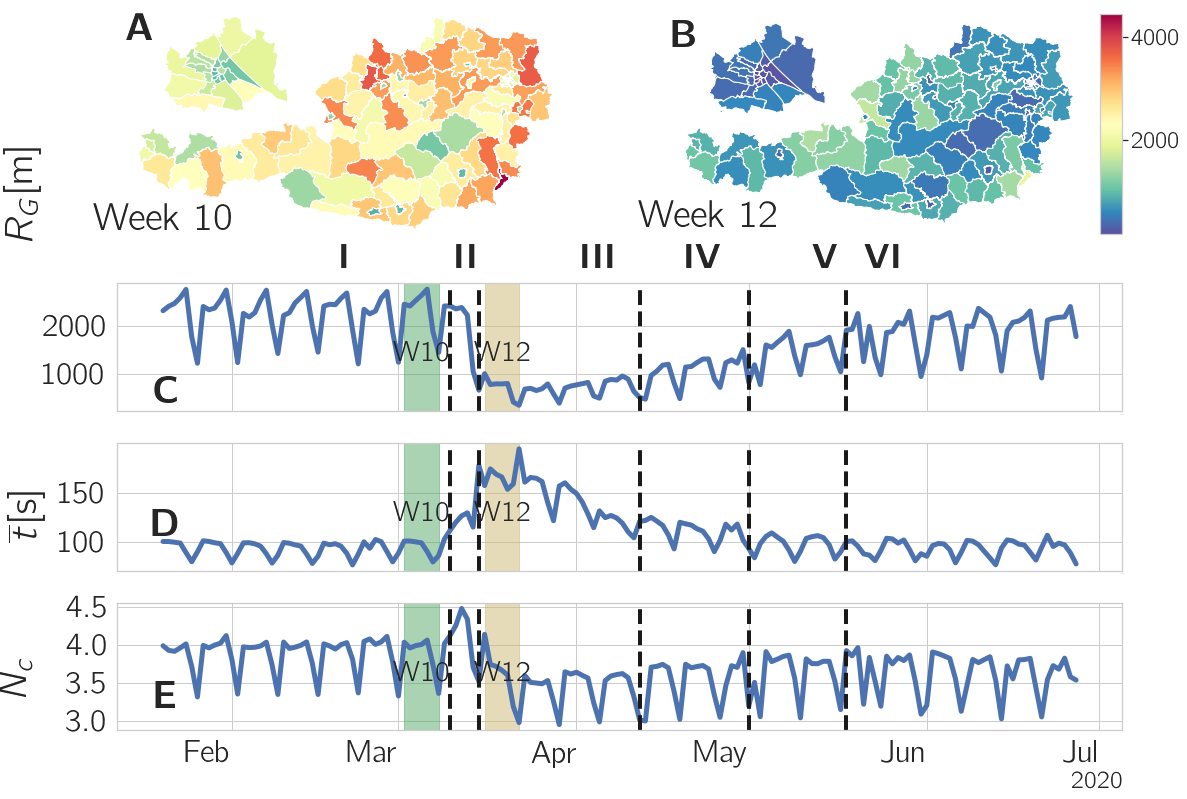
Figure 1: Population-wide response to the COVID-19 crisis. The maps show the mobility (radius of gyration, $R_{G}$) for calendar week (A) 10 and (B) 12 for Austria. The timeseries below outline the changes in (C) $R_{G}$, (D) the call duration per call $\bar{t}$, and (E) the number of calls per device $N_{c}$. During the lock-down mobility was drastically reduced throughout Austria. The call duration per call $\bar{t}$ increased dramatically and the number of calls, after a brief increase around the beginning of the lock-down, dropped below the pre-lock-down level.

Gender differences in human mobility and communication have been reported in palchykov2012sex ; gauvin2020gender . In palchykov2012sex changes in communication behavior across age and gender were reported and how reproductive investments and preferred relationships of both sexes shift over a lifespan. It is well known that males tend to have a workplace further away from home and thus generally move more, see e.g. prashker2008residential . Gender differences in mobility in Santiago de Chile are reported in gauvin2020gender . There, significantly different movement behavior is found which is interpreted as an interplay of socio-economic and urban factors. The gender specific behavioral response to seven terrorist attacks in six cities is investigated in juul2020gender . They compare mobile phone communication patterns in response to the attacks and report significant differences between the genders.

Results

We partition the observation period from February 1^st to June 29^th 2020 into six periods: I Pre-awareness phase. The population is practically not yet aware of the presence of the disease in Austria. II Transition period from the announcement (March 12^th) to the actual lock-down on March 16^th. III lock-down until first easing of NPIs (April 13^th). IV Period of some easing of NPIs. V Gatherings of more than 10 people are allowed, begins on May 1^st. VI Back to normal, restaurants and businesses re-open. For more details, see SI Text S1. We analyze 454,000 women and 452,000 men, for a description of the data see SI Text S2.

Overall behavioral changes during the lock-down

Figure 1 shows the effects of the lock-down. A reduction of mobility in the districts of Austria occurs from before the lock-down (panel A) to right after it (panel B). As a measure for mobility we use the median radius of gyration, $R_{G}$, see Methods in SI Text S3. $R_{G}$ captures the time weighted, spatial extent of an individuals trajectory. We observe a decrease of $R_{G}$ between 59% and 14%. Panel C shows the time evolution of $R_{G}$, averaged over all districts. After a sharp decline of almost 50% in phase III a rebound to almost pre-crisis levels is seen. In panel D we observe a more than 60% increase of call duration per call, $\bar{t}$. For a definition, see Methods, SI Text S3. Panel E shows a brief increase of the number of calls per person, $N_{c}$, in the days just before the lock-down (phase II) followed by a 10% decrease. We now stratify these changes with respect to gender and age.

Communication patterns

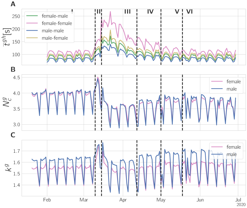
Figure 2: Gender-specific changes in communication behavior. (A) Median call duration of the four possible types of gender-specific calls, depending on who initiated the call and who received it. By mid-May pre-crisis levels are reached. Half-life times range from 17.3d in the female-female to 14.9 in the female-male case. (B) Number of calls originating from males (blue) and females (red). The median call duration peaks in phase III, particularly for female-female calls, whereas the number of calls assumes a minimum. Up to the end of the observation period, pre-crisis levels are not reached. (C) The number of communication partners, the degree $k^{g}(t)$, rises briefly and then drops below pre-crisis levels.

As proxies for the strength of social interactions we first analyze the call duration per pair of interaction partners, $\bar{t}^{gh}(t)$, the number of calls, $N^{g}_{c}(t)$, and the number of calling partners per user, $k^{g}(t)$, see Methods in SI Text S3. The superscripts indicate gender, $g$ represents the gender of the caller $h$ is the gender of the called.

Figure 3: Gender ratios of communication and mobility for different age cohorts. The gender ratio of (A) the median call duration $\bar{t}$ and (B) the radius of gyration, $R_{G}$, is seen. In III the $R_{G}$ gender ratio of young cohorts is shifted towards women moving significantly (p ¡ 0.001) less, while for old cohorts it is shifted towards a more balanced value. In the same period, for all cohorts except 75+, the gender bias for the call duration increases towards women that have a higher call duration.

Figure 2 depicts the situation over time. In panel A we see a massive increase of calling times for the different gender combinations in phase II and the beginning of III. For the female-female calls we observe an increase of up to 140%, female-male and male-female rise by up to 81% and 97%, respectively, and male-male calls increase up to 66%. We find that calls involving women are generally longer than those involving men. Moreover, the call time increase is larger when women are involved.

Calling times decrease gradually and reach pre-crisis levels in phase VI. This decay can be fitted with an exponential function. The exponents of the fits translate into corresponding “half-life” times, which are $t_{1/2,mm}=15.9$d for male-male and $t_{1/2,ff}=17.3$d for female-female interactions, the mixed interactions have half-life times of $t_{1/2,mf}=15.5$d and $t_{1/2,fm}=14.5$d for male-female and female-male interactions, respectively. For details, see SI Text S4. Call times show a pronounced bias towards female initiated calls being longer. In phase I, female originated calls were 10% longer than male originated, and up to 30% longer on weekdays in phase III. From its maximum in phase III, the gender ratio continuously declines to normal levels in phase V, see Supplementary Fig. 15 A.

The age profile for the median call duration is relatively flat for the adult and senior age cohorts and has very low values for the youngest cohort. The call duration increases slightly for the two youngest, but strongly for the two oldest cohorts. For a visualization, see Supplementary Fig. 17. The gender ratio in call duration is biased towards women for all ages during the crisis, as seen in Fig. 3 A. Notably, the age cohort 15-29 is the only cohort having a more balanced call duration on weekends. For all other cohorts gender differences are increased on weekends. Around the beginning of phase III, the ratios for all except the 75+ cohort reach a maximum. The 75+ cohort reaches a maximum of the gender imbalance in phase IV.

In Fig. 2 B we show the number of calls, $N^{g}_{c}$, for male and female generated calls. After a short increase in calls in phase II (female: +13%, male +6%) we see a significant drop in calls in phase III (both -9%), which never reaches pre-lock-down levels in the observation period. It stabilizes at a level of -5% and -4% of the previous level for women and men, respectively. There are only small gender difference in the number of calls. For a discussion see SI Text S5.

In Fig. 2 C we show the timeseries for the number of different communication partners, $k^{g}$, i.e. the degree of men and women in their communication networks. After a brief rise (up to 8% and 13% for men and women, respectively) in phase II, $k^{g}$ falls below its pre-crisis level (-3% and -2%). In phases IV and V $k^{g}$ rises to values higher than the initial values in phase I. In phase VI $k_{g}$ is about 4% higher for men and 2.5% higher for women.

During normal times (phase I) we find that men have a slightly higher average degree (communication partners) on weekdays (f/m ratio 95%, men 1.6, women 1.55 unique contacts per day), while on weekends it is more or less balanced (women and men 1.4). In phase II, $k_{g}$ is increased for both genders to a maximum around 1.73, with an increasingly smaller gender bias. In phase III the degree drops below pre-crisis levels, but men reduce $k^{g}$ stronger, resulting in a smaller gender divide in phase III (96%). From phase IV onward, the degree slightly increases (even above pre-crisis levels: men 1.7 and women 1.6), even stronger for men, hence resulting in an increased gender divide (less than 94%). Supplementary Fig. 16 C shows the age dependence of the gender ratio for the degree. Again, there is a weekend trend towards women. They have more communication partners on weekends, except for the 15-29 age cohort. The gender ratio increases in phase III for all age cohorts.

Call duration increases much more than the number of calls decreases, regardless of gender. This is visible in Fig. 1 D and E. Just in phase II there is a drastic rise in both, call time per call, and the number of calls. The concentration of communication partners is higher for females and increases during crisis. The bias is also shifted towards men having more communication partners in phase VI. All proxies indicate a strengthening of individual contacts and a focus on important contacts.

Gender ratios of different phases are compared with a two-sided Mann-Whitney-U test and reject the null hypothesis that they are from the same distribution. The results of the significance tests are presented in SI Text S6 for all age groups, separated into weekdays and weekends.

Mobility

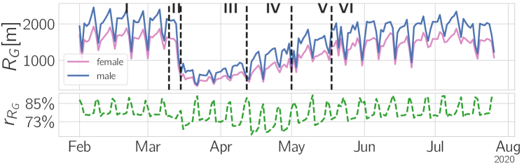
Figure 4: Mobility quantified by $R_{G}$. The upper panel shows $R_{G}$ for men (blue) and women (pink). The lower panel depicts the gender ratio, $r_{R_{G}}$, over time. We observe a large drop in $R_{G}$ for both genders in phase III and a drop in gender ratio in phases III (lock-down), IV, and V (lock-down eased).

In Fig. 1 C we see the overall decline of mobility in terms of the radius of gyration, $R_{G}$. Austrians move drastically less during the lock-down, start to move again when the first easing occurs in mid April, and return back to normal in phases V and VI. Figure 4 A shows $R_{G}$ for the two genders, $R^{f}_{G}$ (red) and $R^{m}_{G}$ (blue). The gender-ratio, defined as $r_{R_{G}}=R^{f}_{G}/R^{m}_{G}$ is depicted in panel B. The female population is moving less than males in pre-crisis times (phase I), as seen in the ratio $r_{R_{G}}$ of 78% on weekdays and 88% on weekends. After a brief transition period II the Weekday ratio drops to around 73% during the lock-down phase III, while on weekends the ratio remains at initial levels. In phase IV, once restrictions were lifted, $R_{G}$ for males returns back to normal more quickly than for females, hence decreasing the gender ratio further down to 67%. The ratio starts to recover towards pre-crisis levels starting from phase V onward, once the main restrictions were lifted. When fitting the $R_{G}$ curves as they converge to pre-crisis levels after the lock-down, we report a half-life time for men of $t^{m}_{1/2}=34.8$d, and $t^{f}_{1/2}=36.0$d for women. For details of the fitting, see SI Text S2.

The changes in gender ratios of $R_{G}$ are significant between the phases. For the significance tests, see Supplementary Tab. 5 in SI Text S6. Especially the changes from phase I to the subsequent phases and from III to phase IV are indeed highly significantly. We find similar results if we replace the radius of gyration by an alternative measure for mobility that is inspired by entropy, $S^{f/m}_{i}$. It is presented and discussed in SI Text S7.

In Fig. 3 B we show the age-stratification of the gender-ratios. Before the crisis we observe very different gender ratios for different ages. Generally the ratio decreases with increasing age. For the young cohort of 15-29 years, the weekday-ratio is above 90%. For the two age cohorts above the average age of first childbirth, 30-44 and 45-59, the ratio is reduced to about 83%. For the age cohorts of retirement, 60-74 and 75+, gender disparity becomes even more biased towards men with a ratio of about 70%. In phase III, the three younger cohorts show an overall trend of increasing gender biases. For the age cohort 45-59, this trend is much less pronounced. Strikingly, the effect is reversed for the retirement cohorts where the gender ratio changes from around 70% to more than 80%, which again decreases towards pre-crisis levels in phase IV. The ratio for the old cohorts returns much more quickly to pre-crisis values than all the younger ones, which do not return to the previous values until the end of the observation period. We do not observe large differences in half-life times across gender, but $t_{1/2}$ is much smaller for older cohorts. For all cohorts we find values between $t_{1/2}=38.8$d for 15-29 year old women to $t_{1/2}=28.8$d for 75+ year old men. For more details, see SI Text S2. For the corresponding statistical tests, see SI Text S6.

For the radius of gyration, we can compare it with data of the previous year (2019) along the same time period. We find that in 2020, during the lock-down phase, there is less than 40% of the movement than in 2019, see SI Text S8.

Basic provisioning

In SI Fig. 22 A we show the number of unique devices as a proxy for the number of people at a shopping center across the lock-down. We count the number of unique subscribers in a specifically defined area, see SI Text S3 for the exact definition. In panel B the corresponding gender ratio is shown. The shopping center is the largest of its kind in Austria and one of the largest in Europe. It is a cluster of 359 shops spread over an area of 670,000 m². Shops sell a wide range of products, including sports equipment, garments, furniture and electronics. It is visited by more than 20 million visitors each year from Vienna and its hinterland, especially in the south, as well as from Hungary and Slovakia. There are also 14 shops, including supermarkets, drug stores and pharmacies that were not affected by the lock-down.

The visiting patterns of the shopping center in phase I show a pronounced weekly periodicity with a maximum on Saturdays and very few visitors on Sundays, when all stores except cinemas and restaurants are closed. The gender ratio in phase I is close to one, indicating gender balance. In phase III the shopping complex was shut down to a large extent. No businesses other than stores for basic provisioning were allowed to open. Nevertheless we find a small number of visitors that we account mainly to persons shopping for food and drugs. The gender ratio in phases III and IV is clearly male-dominated (see Fig. 22 B and for p-values, see SI Tab. 7 in SI Text S10). In phase V, when shops were allowed to re-open, visitor numbers rose to pre-crisis levels at the beginning of the week, however without the strong peaks on Saturdays. The gender ratio returns to a balanced situation; compare with SI Tab. 7. For a comparison with the same period in 2019 we refer to SI Text S9.

Leisure activities

In SI Fig. 24 A we count the numbers in a popular recreational area nearby Vienna, the Kahlenberg, frequented mainly for walks, and easy hikes. The number of visitors does not drop in phases II–V, but increases with the usual seasonal trend from March to June. For a comparison with the situation in the year 2019, see SI Text S11. We find more visitors on weekends and on days with good weather, explaining the high variance in numbers. The gender ratio is biased towards women during phase I, which changes in phase III, where we find a more balanced gender ratio. Interestingly, the gender ratio does not return to pre-crisis values after the lock-down, see SI Fig. 24 B. The corresponding statistical tests are found in SI Tab. 7 in SI Text S10.

Circadian rhythms

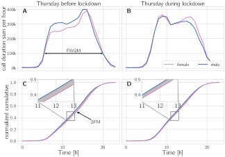
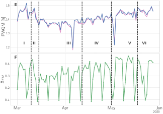
Figure 5: Changes in circadian rhythms during the lock-down measured by the call duration (in seconds) in the whole network. (A) Phone network traffic measured by call duration per hour on the last Thursday in phase I, March 4^th. The horizontal arrow marks the full-width-quarter-maximum length (FWQM). (B) Call duration per hour on Thursday, March 18^th, the first Thursday in phase III. (C) Normalized cumulative activity for the day shown in panel A. The inset highlights the difference of the male and female curve. The gray shaded area marks the difference between the circadian rhythm of men and women, denoted by $\Delta_{FM}$. (D) Same as in C, but for the curve in panel B. (E) FWQM for men and women over time. (F) As the gender ratio of FWQM does not change significantly, we show the gender difference in circadian rhythm, $\Delta_{FM}$, over time. For both genders, the activity maximum shifts from late afternoon to morning and the length of the activity period is approximately 45 minutes shorter during the lock-down. A reduction in $\Delta_{FM}$ means that circadian rhythms of men and women become more synchronized.

We compare aggregated phone network traffic across the 24 hours of a day for women and men, to estimate gender differences in circadian rhythms. For definitions, see SI Text S3. Figure 5 A and B show the call time per hour for the last Wednesday in phase I and the first Wednesday during the lock-down. The maximum activity shifts from the late afternoon to the morning hours. The average full-width-quarter-maximum (FWQM) captures the length of the daily activity period. We find that the FWQM is reduced by approximately $53$ minutes from $14\textrm{h}33\textrm{min}$ in phase I to $13\textrm{h}40\textrm{min}$ in phase III. The results are displayed in panel C. We do not find a significant change in the gender ratio of the activity FWQM (Mann-Whitney U, $p>0.05$).

To capture the shift of the activity of men and women to different times of the day, we calculate the normalized cumulative functions of the call duration, as shown in Fig. 5 C and D, thereby correcting for different total activity. Following juul2020gender we compare gender differences by calculating the area between the curves $\Delta_{FM}$, see Fig. 5 C by the gray shaded area, see Methods in SI Text S3. A large (small) value indicates that the activity of men and women takes place at different (the same) times of day. We find that $\Delta_{FM}$ reduces by 25% from phase I to phase III. The values for FWQM and $\Delta_{FM}$ across the crisis are shown in panels E and F. The significance of these findings is again shown with a two-sided Mann-Whitney U test that rejects the null-hypothesis that the values are drawn from the same distribution with $p<3\times 10^{-5}$. It confirms that $\Delta_{FM}$ is indeed lower in phase III.

Qualitatively we find the same behavior for the sum of gigabytes up- and downloaded and the number of calls. The reductions in lengths of day range from 40 minutes for the downloaded gigabytes to 60 minutes for the number of calls. For the corresponding analyses, see SI Text S12

Discussion

The COVID-19 pandemic represents a unique natural experiment to understand individual and collective coping mechanisms with respect to stress and crisis. Telecommunication data reveals almost real-time insights into many aspects of daily life without interfering with the subjects’ actions and interactions. Using anonymized mobile phone data of a large fraction of the Austrian population, we find that gender differences that exist in communication patterns, mobility and spending leisure time are amplified during the crisis, imposed by a severe lock-down in the first phase of the COVID-19 crisis. In the context of basic provisioning, we find that during the crisis there is a bias toward men doing the shopping for food that is absent in normal times. For circadian rhythms we see that the daily activity is concentrated on a shorter period of the day for men and women equally and that the circadian rhythm of men and women becomes more synchronized during the lock-down.

For both genders we observe an increase in total call duration, which is due to an increase of the call time per call and interestingly a decrease in the number of calls. This is a clear sign that conversation focuses on the core communication partners. This result is in line with a general decline of the number of communication partners during the lock-down. The reduction in communication partners could also result from the loss of conversation partners from work, but we also observe a reduction on the weekends, where we would not expect the effect of work to dominate. The degree distribution before the crisis is in line with earlier work on mobile phone data onnela2007structure . While they find a mean degree 2.34 (averaged over 18 months), we get a smaller value of 1.53 because we average over 24 hours. However, we find the same power-law exponent $\sim-8$ for the degree distribution. In these quantities we see a clear increase and amplification of the gender-biases.

Women show a smaller decrease in the number of calls and a stronger increase in call time per call. As a consequence, the gender ratios of both quantities shift towards females. Women have been reported to have more tightly knit (online) networks than men szell2013how ; igarashi2005gender . We interpret our findings as a signal that this behavior intensifies during crisis. Additionally, our findings agree with the well known tend and befriend reaction, which says that facing (real or perceived) danger, females are more likely to defend offspring (tend) and turn to their social group for protection (befriend) taylor2000biobehavioral . The tightening of the social network can also be attributed to social carework, such as calling lonely elderly, which is performed more often by women during the lock-down prainsack2020solpan . Women were reported to employ more active, problem-oriented coping strategies such as emotional and social support, while men show rational and detachment strategies ben1996gender ; matud2004gender , again supporting the expectation, that women seem to tighten their social networks more than men.

We find that the recovery time to women’s total call time initially is as fast as for men, but later on clearly slows down. The higher, longer increase in demand for communication can be interpreted in the context with higher needs for communication as a coping strategy in an ongoing crisis ben1996gender ; matud2004gender . It also aligns well with the fact that women experience more stress than men michael2009gender , have higher levels of post traumatic stress disorder stein2000gender and have a higher prevalence to depression, partly due to ‘stress responsiveness’ parker2010gender . Our result could be confounded by gender differences introduced by work environments. However, increasing gender-ratios in the call times per call and the number of calls on weekends are a strong indicator that the confounder indeed weakens the effect on weekdays.

The age profiles for call times and the number of calls seemingly suggest that younger cohorts communicate less than older ones. We attribute this to the increased use of instant messaging services torok2016big and other modern channels of communication by the younger cohorts. Here a channel selection bias towards younger cohorts using web-based communication services more actively acts as a severe confounding factor.

The female population is moving less over the entire period, confirming earlier work in different countries and situations gauvin2020gender ; prashker2008residential . The decrease in mobility following the lock-down is stronger for women. In addition, men recover their mobility behavior much quicker after the measures are lifted. This effect depends on age. For the young and adolescent population the existing gender-bias in mobility is enhanced, while for those above retirement age the bias reduces. We relate this to childcare duties during the reproductive age and gender specific differences in occupation. This confirms the apprehensions that females would be required to restrict their mobility stronger due to childcare duties and higher unemployment ifes2020homeoffice ; Viglione2020 ; oecd2020women .

In addition to care-taking duties, we expect more effects. Women were shown to exhibit more ethical behavior, at least where it is socially desirable, while men often behave less community-aware betz1989 ; dalton2011 . For women, it has been shown that they are 50% more likely to adopt non-pharmaceutical interventions in response to a respiratiory epidemic moran2016meta . In this context, the reduction of mobility in women could be partly attributed to responsible behavior in staying at home to protect vulnerable parts of the population. This argument is supported by a qualitative panel survey, that reports women taking the COVID-19 pandemic more seriously in Austria eberl2020die ; kittel2020austrian .

Since it seems that men go out for work more and are more often responsible for gathering basic provisions during the lock-down, they are more exposed to the perceived danger of catching SARS-CoV-2. This could be interpreted as increased risk-taking behavior in men, in line with gustafsod1998gender ; byrnes1999gender ; szell2013how .

Generally, gender differences in mobility decrease on week-ends. We confirmed that the radius of gyration is larger for men because they commute more/farther gauvin2020gender . This suggests that a main factor for our observed behavioral changes is indeed driven by work. Further evidence for this hypothesis is found in the fact that only for the 60+ age cohort the gender-ratio does not change between weekends and weekdays. Nevertheless, the effects discussed above persist on weekends and our conclusions stay valid.

We proxy the activity of people by analyzing their Internet traffic loads across a day. On average, the daily activity period, as observed by several quantities, is reduced by around 40 to 60 minutes by the lock-down. The gender-ratio of the length of a day does not change significantly. However, mobile phone usage of men and women takes place at different times of the day, with the maximum shifted from the late afternoon to the morning during the lock-down. Network traffic starts to increase later in the day and ends earlier. This can be explained by commutes becoming obsolete because of home office and the rise in unemployment ifes2020homeoffice ; Viglione2020 ; oecd2020women . We believe that the shift of the maximum activity from evening to morning is on one hand caused by different activity patterns in home office and by different spare time activities during the lock-down.

The gender-difference in cumulative activity, correcting for different activity levels, drops by 25%, hence showing that the circadian rhythms of women and men become more synchronized during the lock-down. We interpret this as a consequence that people stay at home much more than usual, where often an opposite-gender partner is present statistikaustria2020lebensformen . It would be interesting to understand if the synchronization is stronger for couples spending much time together. More detailed studies of the effects of the pandemic on the circadian rhythm, with respect to age and personal attributes, such as morningness or eveningness aledavood2015digital , could give more detailed insights in e.g. disturbed sleep patterns.

We have shown that massive collective crisis results in tighter social networks with a focus on a social core environment. Women seem to focus more on this tightening, indicating stronger, more active coping strategies, a different perception of the dangers of COVID-19 and stronger pro-social behavior. We see that mobility is reduced much more in females, and the time to recovery is much slower for females. This is partly connected to work-related influences and maybe a stronger community-aware behavior in response to public mobility restrictions. We might see a slight indication of increased risk taking in males when it comes to basic provisioning. Finally, we report synchronization effects of (electronic) activity behavior during the day between males and females during crisis.

Methods

For a description of the data set see SI Text S2 and for definitions of the used metrics see SI Text S3.

I.1 ACKNOWLEDGEMENTS

We thank Eva Bauer, Barbara Prainsack, Christian Diem, and Hannah Metzler for helpful discussions. This work was supported in part by Austrian Science Fund FWF under projects P29252 and I3073, the Austrian Research Promotion Agency (FFG) under projects 857136 and 873927, the WWTF under projects COV 20-017 and COV 20-035, and the Medizinisch-Wissenschaftlicher Fonds des Bürgermeisters der Bundeshauptstadt Wien under project CoVid004.

.

Supplementary Information

SI Text S1: Partitioning of observation interval

The observation period ranges from Feb 1 to June 29 2020. Our analyses compare various periods of time before, during and after the lock-down. Each period is based on the introduction or easing of one or more non pharmaceutical interventions (NPIs) and identified by roman numerals. Period I refers to the phase before the Austrian population was widely aware of the COVID-19 disease in Austria, and ends with the first press conference announcing public restrictions such as school closings and a call for home office on March 12^th.This was followed by a transition period II until Sunday, March 15, 2020, when an extensive lock-down was announced Including all shops closing and restrictions on public movement and gatherings, such as public transport only being allowed to be used for commuting, a ban on meetings with non-household persons and leaving the home only permitted for work that cannot be postponed, grocery-shopping, helping people and short walks. The following lock-down III lasted until Easter (April 13, 2020) which marks the first easing of the measures with small shops and construction stores being allowed to re-open. Phase IV continues until the beginning of phase V on May 1, where the lock-down was eased further and gatherings of up to 10 people were allowed. May 15^th marks the beginning of phase VI, with restaurants and bars re-opening. The dates and description of the measures is based on Desvars-larrive2020 .

SI Text S2: Data

We partnered with a large Austrian internet service provider (ISP) to get access to data from mobile phones. We use a combination of classical Call Data Records for the voice domain as well as X Data Records for the data domain. Thus we do not only register an event when a call is performed, but rather perceive additional events when data packages are transferred. Various network interfaces are connected via probes so we get data points from a multitude of network technologies for mobile data usage (2G, 3G, 4G), calls, text messages as well as Voice over LTE, from both user- as well as control plane. On average we observe approximately 1 Billion events per day, 4.5 Million devices per day and for 80% of the devices the next event is received in 1.7 minutes, on average 4 minutes. When evaluating gender differences we need to filter the data to approx 1.2 Million devices per day where demographic details are defined. Demographic information is not available for roamers or virtual mobile operators (MVNO) and thus they are excluded from this analysis. Furthermore, only devices with a radius of gyration $R_{G}$ (see eq. (1) below) larger than 0m and lower than 300km are considered to exclude resting internet of things-devices and devices above the theoretical maximum of $R_{G}$ in Austria. Calls are filtered to a length of at least 25 seconds prior to aggregation to exclude calls that were not picked up, which form a distinct peak just below 25 seconds, shown in Supplementary Fig. 6.

As the gender attribute in the data set is self-reported and we discuss psychological, social and biological reasons for the observed behavioral changes, we will use the term ‘gender’, referring to the psycho-social construct.

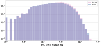
Figure 6: Histogram of the call duration. There is a local maximum around 25 seconds, corresponding to calls not answered, which we get exclude by introducing a cutoff at 25s. Note the double logarithmic axes.

Table 1 outlines the distribution of the devices per cohort. As not all devices are active every day we give the mean and standard deviation as an approximation for the overall counts. As we cannot analyze a device for more than 24 hours (see below), we need to calculate aggregate statistics over the analyzed time period.

Table 1: Sample sizes of the gendered demographic cohorts.

gender	age group	mean	std
female	15-29	44318	3038
female	30-44	130137	9349
female	45-59	151173	11576
female	60-74	80479	6269
female	75 +	18890	1726
male	15-29	42023	2553
male	30-44	116230	7493
male	45-59	158313	12686
male	60-74	84800	7368
male	75 +	19085	1915

Localization

Our localization methodology is based on the topology of the network, namely the observed cell-id. This means that the accuracy is limited, and much less accurate than GPS based localization or the result of custom apps combining Bluetooth, WiFi and GPS. However, the data is available for a large quantity of devices. The ISP provides us with the localization information for each cell-id, which is based on the centroid of the network coverage simulation.

Privacy

The data is anonymized, any identifiers are hashed every 24 hours with a changing key by the ISP prior to making the data available for the researchers. Only cell-id based localization is used to enhance the privacy of the subscribers and only aggregate and k-anonymized statistics are reported. With this procedure we adhere to the recommendations of the GSMA gsmacovid with regards to data privacy handling as well as the law of the local jurisdiction.

SI Text S3: Metrics

Communication

By analyzing calls, social interactions can be modeled. This part of the data consists of a list of outgoing (MO) and incoming (MT) calls, each associated with a source and destination. We filter to calls with a duration of at least 25 seconds to adjust for a shift in the distribution corresponding to calls that were not answered (see Fig 6).

For each device we find $N_{c}^{\mathrm{MO}}$ outgoing and $N_{c}^{\mathrm{MT}}$ incoming calls with $k^{\mathrm{MO}}$ and $k^{\mathrm{MT}}$ other individuals, respectively (in- and out-degree). The call duration is denoted by $\bar{t}$. Additionally, as described earlier for the mobility dimension, for each device, age group and gender are specified.

For all of these device-level metrics we report the median of the whole population, or for cohorts specified by age groups or gender. We will add superscripts $g$ and $h$ to indicate gender.

Mobility

We obtain mobility data as a stream of spatially localized network signaling events. It is transformed into a list of locations $\vec{x}_{i\mu}=(x_{i\mu},y_{i\mu})$, with associated stay duration $t_{i\mu}$ for every individual $i=1...N_{indiv}$ at location index $\mu=1...N_{locations}$, where $x$ and $y$ represent longitude and latitude, respectively. Due to the anonymization procedure the location index $\mu$ is reset every day and the individual index $i$ is reshuffled accordingly. For the individuals, metadata is collected in a vector $m_{i}=(g_{i},a_{i})$, containing gender $g_{i}\in{female,male}$ and age $a_{i}$ aggregated into cohorts of 15 years.

The radius of gyration $R_{G}$ is calculated as the square root of the time-weighted mean of the squared distances $d$ of the locations $\vec{x}_{i\mu}$ to the daily centroid $\overline{x}_{i}=\frac{\sum_{\mu}\vec{x}_{i\mu}t_{i\mu}}{\sum_{\mu}t_{i\mu}}$:

$$R_{\mathrm{G},i}=\sqrt{\frac{\sum_{\tau}d(\overline{x}_{i},\vec{x}_{i\tau})^{2}}{\sum_{\tau}t_{i\tau}}}$$ (1)

It captures the amount of movement in a time weighted manner and has the dimension of a length in meters. The distribution of $R_{\mathrm{G},i}$ is fat tailed, see Fig. 7. In the main paper we report the median because it robust to heavy tails.

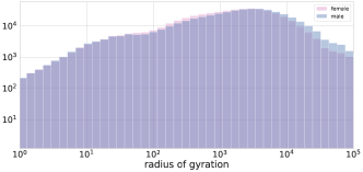
Figure 7: Histogram of the radius of gyration $R_{G}$. Note the double logarithmic axes and the truncated fat tail.

For our second mobility measure entropy the locations $\vec{x}_{i\mu}$ are binned into a hexagonal raster using Uber’s H3 uber_h3 . The chosen resolution level for the raster yields hexagons with an area of approximately $800m^{2}$. For each hexagon $\tilde{x}_{\nu}$ ($\nu=1...N_{hex}$), the stay duration of the locations in each hexagon are aggregated to $\tilde{t}_{i\nu}$

$$\tilde{t}_{i\nu}=\sum_{\nu\forall\vec{x}_{i\nu}\in\tilde{x}_{\nu}}t_{i\nu}$$ (2)

The stay time distribution of an individual $i$ is then defined as the share of its time spent in a given hexagon $\tilde{x}_{\nu}$

$$p(\tilde{x}_{i\nu})=\frac{\tilde{t}_{i\nu}}{\sum_{\nu}\tilde{t}_{i\nu}}$$ (3)

The entropy of an individual’s stay time distribution, $S_{i}$, is defined, using the standard formulation of Shannon Entropy, as:

$$S_{i}=-\sum_{\nu}p(\tilde{x}_{i\nu})\log_{2}(p(\tilde{x}_{i\nu}))$$ (4)

Points of interest (Shopping, Leisure)

Specific points of interest reflecting shopping and leisure zones in Vienna were analyzed in more detail. We first used H3 by Uber uber_h3 to create a discrete raster for the whole country to speed up the analysis of specific locations afterwards. Then we count the number of unique subscribers in a set of manually defined hexagons. We limit our investigations to stays longer than 10 minutes and shorter than 4 hours. We assume this eliminates devices passing the shopping complex on the nearby highway, as well as persons working there, because these activities take much shorter or longer, respectively.

Circadian rhythm

We investigate the circadian rhythm using network traffic measures $A(t)$ aggregated by gender and ranging from the sum of call duration per hour to downloaded gigabytes per hour. Irrespective of the quantity, we observe a broadened, peak-like structure with a rise in the morning and a drop in the evening. We quantify the duration by the full-width-quarter-maximum distance (FWQM). It denotes the time span between point where the activity is larger than the quarter of the maximum activity in the morning and the point where the activity drops below the same value in the evening. We choose the threshold relative to the maximum, so we are independent of the total activity; its value is set to a quarter without loss of generality.

$$A(t)-max(A(t))/4=0\quad\forall t_{1},t_{2}$$ (5)

$$\mathrm{FWQM}=t_{2}-t_{1}$$ (6)

Male and female activity, corrected for the difference in total activity, is not distributed across the 24 hours of a day in the same way. Inspired by juul2020gender we apply the following procedure. We correct for the difference in total activity by calculating and normalizing the cumulative activity

$$C(t)=\frac{\int_{0}^{t}A(\tau)d\tau}{\int_{0}^{24}A(\tau)d\tau}\quad\textrm{,}$$ (7)

where 0 and 24 are the time at the beginning and end of the chosen 24 hour period. Now we calculate the gender difference $\Delta_{FM}$ in circadian rhythm by calculating the absolute area between the cumulative activity functions for men and women

$$\Delta_{FM}=\int_{0}^{t_{max}}|C_{m}(t)-C_{f}(t)|dt$$ (8)

Gender differences

To investigate gender differences we calculate the gender ratio $r_{x}$ for the various aggregations $x$ presented in this work. The ratio $r_{x}$ is calculated as the quotient of the aggregate for the female cohort divided by the aggregate for the male cohort $r_{x}=x_{\mathrm{female}}/x_{\mathrm{male}}$ ($x$ represents the aggregation, e.g. median $R_{G}$ or median call duration $\bar{t}$). A gender ratio $r_{x}$ close to 1 (or 100%) indicates that the quantity is of similar size for both genders, less (more) than 100% indicates smaller (larger) values for females.

SI Text S4: Time-back-to-normal: Fitting Half-life times

For many of the investigated quantities, the COVID-19 lock-down represents a perturbation from an equilibrium with a subsequent, smooth return to the previous value. We fit an exponential function

$$f(t;a_{0},a_{1},b)=a_{0}+a_{1}b^{t}\mathrm{,}$$

where $a_{0}$ is fixed to the mean value in phase I, $a_{1}$ is the additional offset at the beginning of the decay and $b<1$ is the average daily reduction factor. From $b$ we can calculate the half-life time

$$t_{1/2}=\frac{ln(1/2)}{ln(b)}$$

in days, which quantifies the time it takes the fitted quantity to return halfway back to “normal”. The non-linear least squares fit is performed to the 7-day moving average of the investigated quantity, starting from the beginning of phase III to the end of the observation period. We report standard deviations $\sigma$ calculated as the square root of the diagonal elements of the covariance matrix.

Figure 8: Decay parameters for the call duration $\bar{t}^{gh}$. We show $\bar{t}^{gh}$ (transparent line), the seven day moving average (solid line) and the fitted curve (broken line). The half-life times for the return from perturbed state to normal are 17.3d for male-male, 14.9d for female-male, 15.5d for male-female and 15.9d for male-male interactions. Detailed results of the fitted parameters are in Tab.2.

Figure 8 shows the average interaction time $\bar{t}^{gh}$, its 7-day moving average and the fitted exponential. We find half-life times between 14.9d and 17.3d for female-male and female-female interactions, respectively. The detailed results are given in Tab. 2. The female-female interaction $t_{1/2}$ is more than one standard deviation larger than for the interactions where males are involved.

We also fit for the number of calls $N_{c}$ and the number of unique contacts $k$, see Figs. 9 and 10, and Tab. 2 for details. Both times, the half-life times for females are more than one standard deviation larger. For $N_{c}$ the half-life times are large compared to the other quantities, and in fact it has not reached the pre-crisis levels by the end of the study period.

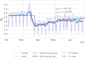
Figure 9: Decay parameters for the number of calls $N_{c}$. We show $N_{c}$ (transparent line), the seven day moving average (solid line) and the fitted curve (broken line). The half-life times for the return from perturbed state to normal are 61.7d for women and 44.4d for men. Detailed results of the fitted parameters are in Tab. 2.

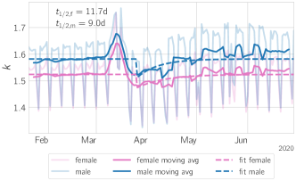
Figure 10: Decay parameters for the number of interaction partners $k$. We show $k$ (transparent line), the seven day moving average (solid line) and the fitted curve (broken line). The half-life times for the return from perturbed state to normal are 11.7d for women and 9.0d for men. Detailed results of the fitted parameters are in Tab. 2.

Table 2: Fitted parameters for the exponential decay. The confidence intervals are one standard deviation.

quantity	gender	$a_{0}$	$a_{1}$	$b$	$t_{1/2}$
$\bar{t}_{i}$	female-female	$107$	$138\pm 4$	$0.9607\pm 0.0015$	$17.3\pm 0.7$d
$\bar{t}_{i}$	female-male	$91$	$69\pm 2$	$0.9546\pm 0.0017$	$14.9\pm 0.6$d
$\bar{t}_{i}$	male-female	95	$81\pm 2$	$0.9562\pm 0.0017$	$15.5\pm 0.6$d
$\bar{t}_{i}$	male-male	81	$52\pm 1$	$0.9573\pm 0.0015$	$15.9\pm 0.6$d
$N_{c}$	female	3.89	$-0.48\pm 0.01$	$0.9888\pm 0.0010$	$61.7\pm 5.6$d
$N_{c}$	male	3.89	$-0.55\pm 0.02$	$0.9845\pm 0.0012$	$44.4\pm 3.5$d
$k$	female	1.524	$-0.052\pm 0.007$	$0.9426\pm 0.0115$	$11.7\pm 2.4$d
$k$	male	1.582	$-0.074\pm 0.014$	$0.9260\pm 0.0198$	$9.0\pm 2.5$d
$R_{G}$	female	1564	$-1331\pm 41$	$0.9809\pm 0.0010$	$36.0\pm 1.8$d
$R_{G}$	male	1959	$-1606\pm 48$	$0.9803\pm 0.0009$	$34.8\pm 1.7$d
$S_{i}$	female	0.73	$-0.53\pm 0.02$	$0.9761\pm 0.0015$	$28.7\pm 1.9$d
$S_{i}$	male	0.78	$-0.52\pm 0.02$	$0.9753\pm 0.0016$	$27.6\pm 1.8$d

We perform the same procedure for the mobility-related quantities radius of gyration $R_{G}$ and stay-time distribution entropy $S_{i}$ and show the fits in Figs. 11 and 12. The results for the fits are reported in Tab. 2. The half-life times of females are slightly, but not significantly larger.

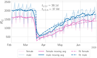
Figure 11: Decay parameters for the radius of gyration $R_{G}$. We show $R_{G}$ (transparent line), the seven day moving average (solid line) and the fitted curve (broken line). The half-life times for the return from perturbed state to normal are 36.0d for women and 34.8d for men. Detailed results of the fitted parameters are in Tab. 2.

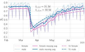
Figure 12: Decay parameters for the stay time entropy $S_{i}$. We show $S_{i}$ (transparent line), the seven day moving average (solid line) and the fitted curve (broken line). The half-life times for the return from perturbed state to normal are 27.6d for women and 28.7d for men. Detailed results of the fitted parameters are in Tab. 2.

For $R_{G}$ we also stratify for age, see Tab. 3.

Table 3: Stratifying the fitted parameters of the exponential function for age. The confidence intervals are one standard deviation.

gender	age	$a_{0}$	$a_{1}$	stdev $a_{1}$	b	stdev b	thalbe	thalbe stdev
female	15.0	2318.96	0.9822	0.0009	-1997	63	38.6	2.0
female	30.0	1809.65	0.9810	0.0009	-1564	48	36.2	1.8
female	45.0	1761.09	0.9810	0.0010	-1446	45	36.2	1.8
female	60.0	1038.4	0.9799	0.0010	-860	27	34.2	1.7
female	75.0	526.376	0.9788	0.0011	-346	12	32.3	1.7
male	15.0	2498.53	0.9819	0.0009	-1948	60	38.0	2.0
male	30.0	2126.9	0.9802	0.0010	-1696	51	34.7	1.7
male	45.0	2089.17	0.9808	0.0009	-1663	51	35.7	1.8
male	60.0	1446.69	0.9791	0.0010	-1195	37	32.8	1.6
male	75.0	786.449	0.9762	0.0014	-610	24	28.8	1.7

Through visual inspection it is clear that the quality of the fits of the mobility quantities are not good because the exponential function does not represent the functional form of the return to normal well. The derivative of $R_{G}$ and $S_{i}$ is small during the lock-down in phase III and gets larger in subsequent phases when the restrictions are lifted. We fit a logistic function of the form

$$f(t;\alpha,t_{0})=\frac{1}{1+e^{-\alpha(t-t_{0})}}\quad\mathrm{.}$$

The turning point, with the largest derivative, is at $t_{0}$ and $\alpha$ controls the time it takes the logistic function to transition from one niveau to the other.

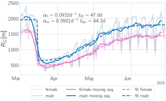
Figure 13: Logistic fit for the radius of gyration $R_{G}$. We show $R_{G}$ (transparent line), the seven day moving average (solid line) and the fitted curve (broken line). The decay rate parameter $\alpha$ is similar for both genders, but the turning point $t_{0}$ for men is earlier than for women with 44.3d and 47.6d after beginning of the lock-down. Detailed results of the fitted parameters are in Tab. 4.

In Fig. 13 we show the results of the results of fitting the step function, the values for $t_{0}$ and $\alpha$ are reported in Tab. 4. The $\alpha$ parameter is not significantly different, but the turning point $t_{0}$ is significantly larger for females.

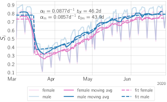
Figure 14: Logistic fit for the stay time entropy $S_{i}$. We show $S_{i}$ (transparent line), the seven day moving average (solid line) and the fitted curve (broken line). The decay rate parameter $\alpha$ is similar for both genders, but as for $R_{0}$ the turning point $t_{0}$ for men is earlier than for women with 43.9d and 46.2d after beginning of the lock-down. Detailed results of the fitted parameters are in Tab. 4.

The same holds for our second measure of mobility, the entropy $S_{i}$. The fits shown in Fig. 14 and values reported in Tab. 4 have not significantly different values for $\alpha$, but the turning point $t_{0}$ for females is significantly later. The extended flat period in the beginning of the logistic function accounts for the extended duration of the lock-down.

Table 4: Fitted parameters for the logistic function. The confidence intervals are one standard deviation.

quantity	gender	$\alpha$	$t_{0}$
$R_{G}$	female	$0.0932\pm 0.0070\mathrm{d}^{-1}$	$47.6\pm 0.8$d
$R_{G}$	male	$0.0901\pm 0.0078\mathrm{d}^{-1}$	$44.3\pm 1.0$d
$S_{i}$	female	$0.0877\pm 0.0078\mathrm{d}^{-1}$	$46.2\pm 1.0$d
$S_{i}$	male	$0.0857\pm 0.0087\mathrm{d}^{-1}$	$43.9\pm 1.2$d

SI Text S5: Further discussion of communication quantities

In this SI Text we provide additional results concerning communication patterns.

The absolute values of the interaction time $\bar{t}^{gh}$ are given in the main text Fig. 2. Here we discuss the gender ratio and stratify for age. Supplementary Fig. 15 A shows the call time female initiated over male initiated ratio $r_{\bar{t}}$ across the six phases. It is typically shifted towards women (+12%) and even more so on weekends (+16%). In the transition phase II the relative gender gap approximately doubles to +27% on weekdays and up to +35% on weekends. Subsequently we observe a smooth return to pre-lock-down values.

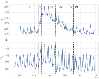
Figure 15: Gender ratios of communication quantities. (A) The ratio $r_{\bar{t}}$ of the call time of female over male initiated interactions starts to spike in II, increases in III and recovers subsequently. (B) The ratio $r_{N_{c}}$ of the number of female over male initiated calls is increased during III, but recovers subsequently.

We stratify for age in Fig. 17 A, where we show the average $\bar{t}^{g}$ over calendar week 10 in phase I and over calendar week 12 in phase III for all age cohorts. The phase I profile is flat with values slightly above 300s for women and slightly below 300s for men. In the lock-down phase III the call time increases for both genders and all ages, but stronger for women and stronger for older age cohorts. The 15-29 cohort increases their communication behavior the least. The gender ratio for $\bar{t}^{g}$ is shown in Fig. 17 B. It is shifted towards women for all age cohorts and the lowest for ages 30-59. We see a strong increase in week 12 for all ages, except the 75+ cohort. In Fig. 16 A we show the time series of the age ratios, already discussed in the main text.

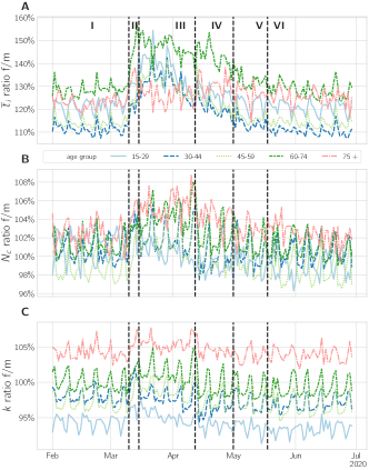
Figure 16: Age dependence of communication strength gender ratios. (A) Gender ratio for call time $\bar{t}$ , (B) gender ratio for number of calls (C) gender ratio for degree. The gender ratios overwhelmingly shift towards women communicating more. The effect is the weakest for the oldest cohort. The youngest cohort 15-29 has a different weekday - weekend pattern than the rest of the age cohorts.

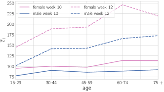
Figure 17: Age profile call duration $\bar{t}$. (A) Weekly average in $\bar{t}$ of week 10 (solid line) and week 12 (broken line). (B) Gender ratio of the weekly average in $\bar{t}$ of week 10 (solid line) and week 12 (broken line). All age cohorts have an absolute increase in $\bar{t}$, but its smallest for the youngest age cohort. The ratio changes only little for the oldest cohort.

Next, we discuss the the number of calls as shown in main text Fig. 2 B. As shown in Fig. 15 B, before the crisis women tended to have slightly fewer calls than men on weekdays (3% less) and more on weekends (2% more). This changes in phase III, where the bias shifts towards women having equally as many calls on weekdays as well as an increased bias on weekends (4% more). The bias returns to normal levels in phase IV, however, the weekday ratio is shifted to be more male-biased. We report significance tests in SI Text S6.

The gender ratio of $N_{c}$, shown in SI Fig. 16 B, deviates only weakly from equality before the lock-down. All cohorts, except 15-29, are biased towards females having longer calls on weekends, except for the 75+ which does not exhibit a weekly rhythm. In phase III the gender ratio for all age cohorts shifts towards women having more calls.

The age profiles in Fig. 18 elucidate this a bit more, by showing that from week 10 to week 12 the number of calls decreased for all age cohorts and especially for young cohorts, which have a higher initial level in week 10. The gender ratio increases from week 10 to week 12 for all age cohorts, except for the cohort 15-29, which remains at the same value.

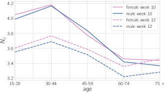
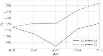
Figure 18: Age profile number of calls $N_{c}$. (A) Weekly average in $N_{c}$ of week 10 (solid line) and week 12 (broken line). (B) Gender ratio of the weekly average in $N_{c}$ of week 10 (solid line) and week 12 (broken line). All age cohorts have an absolute increase in $N_{c}$, but its smallest for the oldest age cohort. However, the ratio changes only little for the youngest and much for the oldest cohort.

Mean degree varies around 1.4 and 1.7, so the range is relatively small. The age stratification in Fig. 19 A shows that degree is highest for the age cohort 30-44. We see that for the age cohorts younger than 45 there is a reduction in degree, for men 45-59 there is a very small reduction and for women older than 45 and men 60+ there is an increase in degree.

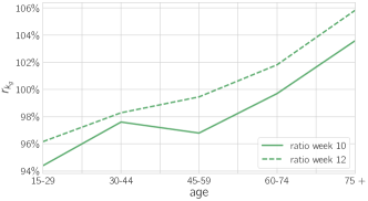
Figure 19: Age profile degree $k_{i}$. (A) Weekly average in $k_{i}$ of week 10 (solid line) and week 12 (broken line). (B) Gender ratio of the weekly average in $k_{i}$ of week 10 (solid line) and week 12 (broken line). This curve is interestingly different from the number of calls in Fig. 18. The absolute values of unique communication partners only increase for younger cohorts and decrease for senior cohorts. Nevertheless, gender ratio rises for all age cohorts.

SI Text S6: Statistical significance of gender-ratio-changes across phases

We perform significance tests to ensure that the changes gender ratio in the observed quantities are indeed significant. Gender ratios of different samples of observables (e.g. phases) are compared with a two-sided Mann-Whitney-U test to reject the null hypothesis that they are from the same distribution. The results are shown in Tab. 5 for the overall quantities and in Tab. 6 we report age stratified tests.

For $R_{G}$ we can show that the reduction from phase I to phases II, III, IV, V and VI is highly significant on weekdays, while the change on weekends is less significant, except for phase IV. The change from before to after Easter, phase III vs. IV is significant as well on weekends and weekends.

Table 5: A Mann Whitney U test was applied to test for significance. We compare the ratio female/male for various metrics of one period against another period, to reject the hypothesis that they are drawn from the same distribution. The following rules were used when assigning the significance stars: $*<0.05,**<0.01,***<0.001$

metric	compared periods	Mann-Whitney
		Weekday	Weekend
$R_{G}$ [m]	I vs. III	3.94e-10, ***	2.69e-01, -
$R_{G}$ [m]	I vs. IV	6.19e-08, ***	6.29e-03, **
$R_{G}$ [m]	I vs. V	3.07e-05, ***	3.95e-01, -
$R_{G}$ [m]	I vs. VI	5.02e-03, **	2.08e-02, *
$R_{G}$ [m]	III vs. IV	1.45e-05, ***	2.02e-02, *
$S$	I vs. III	2.88e-03, **	7.94e-05, ***
$S$	I vs. IV	6.19e-08, ***	4.37e-01, -
$S$	I vs. V	3.31e-04, ***	3.16e-02, *
$S$	I vs. VI	4.19e-04, ***	6.51e-04, ***
$S$	III vs. IV	9.15e-07, ***	2.02e-02, *
$S_{i}$	I vs. III	3.94e-10, ***	2.17e-02, *
$S_{i}$	I vs. IV	6.19e-08, ***	6.29e-03, **
$S_{i}$	I vs. V	7.49e-07, ***	4.64e-03, **
$S_{i}$	I vs. VI	3.27e-01, -	5.78e-04, ***
$S_{i}$	III vs. IV	1.31e-01, -	8.96e-02, -
total call duration (MO) [s]	I vs. III	3.93e-10, ***	2.35e-05, ***
total call duration (MO) [s]	I vs. IV	2.63e-07, ***	7.24e-03, **
total call duration (MO) [s]	I vs. V	3.77e-01, -	3.55e-01, -
total call duration (MO) [s]	I vs. VI	2.13e-11, ***	5.12e-02, -
total call duration (MO) [s]	III vs. IV	9.15e-07, ***	9.81e-03, **
total call duration (MT) [s]	I vs. III	3.94e-10, ***	2.35e-05, ***
total call duration (MT) [s]	I vs. IV	6.19e-08, ***	1.91e-02, *
total call duration (MT) [s]	I vs. V	1.28e-04, ***	3.16e-01, -
total call duration (MT) [s]	I vs. VI	3.55e-07, ***	2.35e-02, *
total call duration (MT) [s]	III vs. IV	1.10e-06, ***	4.44e-03, **
degree	I vs. III	5.97e-04, ***	2.36e-05, ***
degree	I vs. IV	5.88e-06, ***	3.55e-01, -
degree	I vs. V	5.21e-04, ***	3.55e-01, -
degree	I vs. VI	1.34e-07, ***	2.22e-03, **
degree	III vs. IV	3.79e-06, ***	2.91e-03, **

Table 6: Significance testing results per gendered age group for selected metrics. We apply a Mann Whitney U test, comparing the ratio female/male for various metrics of one period against another period, to reject the hypothesis that they are drawn from the same distribution. The following rules were used when assigning the significance stars: $*<0.05,**<0.01,***<0.001$

metric	compared periods	age group	Mann-Whitney
	Weekday	Weekend
$R_{G}$ [m]	I vs. III	15-29	1.18e-09, ***	1.26e-04, ***
$R_{G}$ [m]	I vs. III	30-44	1.18e-09, ***	3.42e-04, ***
$R_{G}$ [m]	I vs. III	45-59	1.68e-09, ***	3.83e-01, -
$R_{G}$ [m]	I vs. III	60-74	2.29e-02, *	8.68e-04, ***
$R_{G}$ [m]	I vs. III	75 +	1.18e-09, ***	4.37e-05, ***
$R_{G}$ [m]	I vs. IV	15-29	1.17e-07, ***	2.19e-03, **
$R_{G}$ [m]	I vs. IV	30-44	1.17e-07, ***	2.19e-03, **
$R_{G}$ [m]	I vs. IV	45-59	1.17e-07, ***	1.24e-02, *
$R_{G}$ [m]	I vs. IV	60-74	1.34e-07, ***	4.28e-01, -
$R_{G}$ [m]	I vs. IV	75 +	5.54e-02, -	3.01e-02, *
$R_{G}$ [m]	I vs. V	15-29	3.94e-05, ***	1.82e-01, -
$R_{G}$ [m]	I vs. V	30-44	3.50e-05, ***	1.51e-01, -
$R_{G}$ [m]	I vs. V	45-59	7.96e-05, ***	4.76e-01, -
$R_{G}$ [m]	I vs. V	60-74	3.29e-03, **	4.76e-01, -
$R_{G}$ [m]	I vs. V	75 +	4.21e-01, -	2.27e-02, *
$R_{G}$ [m]	I vs. VI	15-29	7.57e-07, ***	2.65e-03, **
$R_{G}$ [m]	I vs. VI	30-44	1.69e-02, *	6.02e-02, -
$R_{G}$ [m]	I vs. VI	45-59	1.03e-01, -	1.12e-01, -
$R_{G}$ [m]	I vs. VI	60-74	1.73e-03, **	3.48e-02, *
$R_{G}$ [m]	I vs. VI	75 +	1.68e-10, ***	2.11e-01, -
$R_{G}$ [m]	III vs. IV	15-29	1.93e-01, -	4.72e-01, -
$R_{G}$ [m]	III vs. IV	30-44	5.56e-04, ***	2.81e-02, *
$R_{G}$ [m]	III vs. IV	45-59	1.23e-04, ***	9.81e-03, **
$R_{G}$ [m]	III vs. IV	60-74	6.33e-06, ***	3.85e-02, *
$R_{G}$ [m]	III vs. IV	75 +	1.58e-06, ***	3.85e-02, *
total call duration (MO) [s]	I vs. III	15-29	7.41e-07, ***	7.49e-05, ***
total call duration (MO) [s]	I vs. III	30-44	1.18e-09, ***	4.37e-05, ***
total call duration (MO) [s]	I vs. III	45-59	1.18e-09, ***	4.37e-05, ***
total call duration (MO) [s]	I vs. III	60-74	1.18e-09, ***	4.37e-05, ***
total call duration (MO) [s]	I vs. III	75 +	1.17e-08, ***	2.44e-01, -
total call duration (MO) [s]	I vs. IV	15-29	2.60e-01, -	2.93e-01, -
total call duration (MO) [s]	I vs. IV	30-44	4.48e-07, ***	6.48e-02, -
total call duration (MO) [s]	I vs. IV	45-59	1.17e-07, ***	4.56e-03, **
total call duration (MO) [s]	I vs. IV	60-74	1.17e-07, ***	2.19e-03, **
total call duration (MO) [s]	I vs. IV	75 +	2.31e-07, ***	2.19e-03, **
total call duration (MO) [s]	I vs. V	15-29	1.02e-02, *	3.93e-02, *
total call duration (MO) [s]	I vs. V	30-44	4.09e-01, -	1.82e-01, -
total call duration (MO) [s]	I vs. V	45-59	1.40e-04, ***	3.36e-01, -
total call duration (MO) [s]	I vs. V	60-74	7.48e-04, ***	2.52e-01, -
total call duration (MO) [s]	I vs. V	75 +	6.78e-04, ***	4.28e-01, -
total call duration (MO) [s]	I vs. VI	15-29	1.03e-07, ***	4.90e-03, **
total call duration (MO) [s]	I vs. VI	30-44	1.02e-12, ***	4.05e-04, ***
total call duration (MO) [s]	I vs. VI	45-59	1.43e-03, **	2.81e-01, -
total call duration (MO) [s]	I vs. VI	60-74	3.78e-01, -	3.75e-01, -
total call duration (MO) [s]	I vs. VI	75 +	3.89e-03, **	2.70e-02, *
total call duration (MO) [s]	III vs. IV	15-29	2.16e-05, ***	2.02e-02, *
total call duration (MO) [s]	III vs. IV	30-44	9.15e-07, ***	4.44e-03, **
total call duration (MO) [s]	III vs. IV	45-59	1.32e-06, ***	6.66e-03, **
total call duration (MO) [s]	III vs. IV	60-74	1.57e-06, ***	4.72e-01, -
total call duration (MO) [s]	III vs. IV	75 +	4.49e-01, -	5.19e-02, -

SI Text S7: Alternative measure for mobility: entropy

We calculate an alternative measure for mobility, the entropy $S_{i}$ of the stay time distribution of device i, for a definition see SI Text S3 Methods. A high (low) value of entropy denotes a spread out (concentrated) stay time distribution, i.e. the device was moving a lot (little).

Figure 20: Mobility in Austria, measured by entropy. The upper panel shows entropy $S_{i}$ for men and women, the lower the gender ratio for entropy $r_{S_{i}}$. The drop at the beginning of phase III is very pronounced and so is the change in gender ratio. The weekday gender ratio is shifted towards men moving more and slowly returns to pre-crisis levels.

Figure 20 A shows $S_{i}$ for both genders across the six phases. We observe a very similar pattern as for the radius of gyration. During the week $S_{i}$ is high and on weekends it is significantly less. In phase III $S_{i}$ reaches a minimum and only slowly recovers over the subsequent phases.

The gender ratio of $S_{i}$, shown in Fig. 20 B also corroborates the radius of gyration. In phase I the gender ratio is shifted towards men moving more, an effect which is smaller on weekends. During the lock-down in phase III the ratio is shifted strongly towards men and changed little to nothing on weekends. In phase V the ratio recovers to pre-crisis values.

SI Text S8: Long term analysis

A comparison with the data from the same time period of the previous year is available in Fig. 21. The figure shows the ratio of radius of gyration from 2020 and 2019. If $R_{G}$ was smaller (larger) in 2020 than in 2019, the ratio is less (more) than 100%.

The drastic reduction of movement to approximately 30% compared to the previous year shows the impact of the measures. We also observe that women have a stronger reduction from week 16 to 20.

These results should be interpreted with care, as the accuracy of the localization in the GSM network was improved from 2019 to 2020, potentially resulting in different absolute values of $R_{G}$.

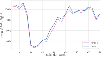
Figure 21: Comparison of the gendered $R_{G}$ with the same time period of the previous year. We plot the quotient of 2019’s $R_{G}$ with 2020’s. During the lock-down the ratio drops below 40%.

SI Text S9: Shopping centers

Here we present the visiting data for a large shopping center in the south of Vienna, as described in the main text. Figure 22 depicts data from the lock-down and is discussed in the main text.

For comparison we analyze the same time from the previous year, 2019, see Fig. 23. In the visitor numbers we find the same weekly pattern as in phase I and a declining trend towards the summer months, which is, nevertheless, much weaker than the reduction in phases III and IV. The gender ratio is quite stable around (or slightly above) 1.

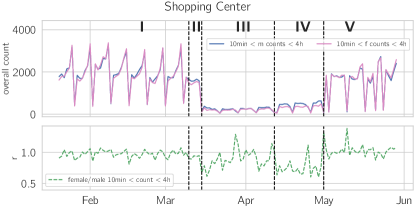
Figure 22: Shopping center in 2020. The upper panel shows the visitor count for a large shopping center in the south of Vienna. In the lower panel the gender ratio for the visitor count in panel A is shown. The lock-down is prominently visible as a drop in the visitor count and a deviation from equality in the ratio.

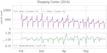
Figure 23: Shopping center in 2019. The upper panel shows the visitor count for the same period as in Fig. 22 in 2019 for a large shopping center in the south of Vienna. The lower panel displays the gender ratio for the visitor count in panel A. The changes from 2020 are not visible in this figure, however a declining trend from February towards summer is present.

SI Text S10: Statistical significance of gender ratio shopping center and recreational area

We perform statistical tests to check if the observed changes in gender ratio from one phase to another are significant. A two sided Mann-Whitney U test is performed to reject the hypothesis that the values in both phases are drawn from the same distribution.

The changes in gender ratio from phase I to phases III, IV and V are are highly significant on weekdays and not significant on weekends.

For the recreational area we find that changes from phase I to phases III, IV and V are highly significant on weekdays and for phases III and IV significant on weekends with a p¡0.01 and p¡0.05 significance level. For the second presented recreational area only the weekday change from phase I to III is significant.

Table 7: A Mann Whitney U test is applied to test for significance. We compare the ratio of female over male count in an area of one phase against another. The following rules were used when assigning the significance stars: *$<$0.05, **$<$0.01, ***$<$0.001.

		Weekday	Weekend
Point of Interest	compared time periods
Recreational Area 1	I vs. III	9.60e-08 ***	7.66e-03 **
	I vs. IV	6.85e-05 ***	1.92e-02 *
	I vs. V	6.63e-08 ***	2.81e-01
	III vs. IV	8.90e-02	3.18e-01
Recreational Area 2	I vs. III	1.68e-03 **	4.85e-01
	I vs. IV	7.24e-02	4.79e-01
	I vs. V	2.03e-01	4.86e-01
	III vs. IV	1.59e-01	2.54e-01
Shopping Center	I vs. III	4.04e-07 ***	1.40e-01
	I vs. IV	2.75e-08 ***	1.11e-01
	I vs. V	3.23e-04 ***	4.59e-01
	III vs. IV	4.72e-04 ***	3.63e-02 *

SI Text S11: Recreational areas

Figure 24 shows the recreational area described in the main text. For comparison we also show the relevant time period in the previous year, 2019, in Fig. 25. The limited comparability due to improvements in the network localization can be seen in the lower number of visitors, compared to 2020. However, the increasing trend towards summer is clearly present. The gender ratio is different to 2020, as it is more shifted towards men, however there is no stark change around march 15^th, supporting the claim that the change from phase I to III is unique to 2020.

To corroborate these findings we analyze a second recreational area on the other side of Vienna, presented in Fig. 26. There the gender ratio in phase I is typically shifted towards more men present. In the beginning of the lock-down, the gender ratio shifts towards equality, while at the same time more devices are present. A comparison with the previous year, 2019, in Fig. 27 shows that these changes are specific to 2020.

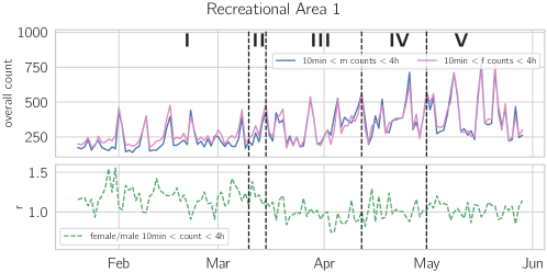
Figure 24: Visitors in a leisure area outside of Vienna, Kahlenberg, during the Covid-19 crisis. The upper panel shows the counts of men and women present in the defined area. The lower panel shows the gender ratio of the counts. The overall counts are unaffected from the lock-down, but the gender ratio changes from being from female-biased to equality.

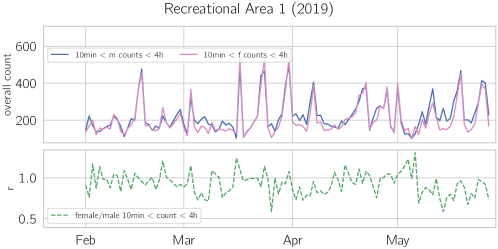
Figure 25: Visitiors in the same leisure area as in Fig. 24, but for the same time period in 2019. The upper panel shows the number of men and women present, the lower panel the gender ratio women over men $r$. We find a weakly increasing trend towards summer, but the gender ratio stays constant throughout the study period. Note that in contrast to 2020 the gender ratio balanced in February and March.

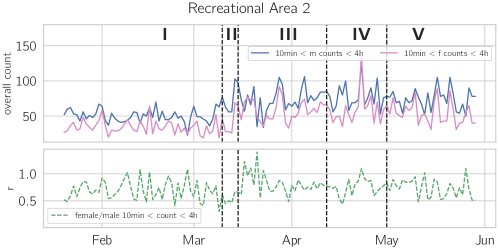
Figure 26: Visitors in another leisure area outside of Vienna, Lobau, during the Covid-19 crisis. The upper panel shows the counts of men and women present in the defined area. The lower panel shows the gender ratio of the counts. The overall counts increase during phase II and stays high until the end of the study period. The gender ratio changes from being from male-biased to being more balanced in phase III.

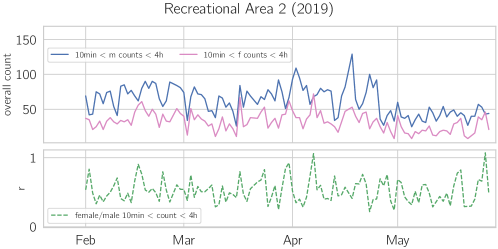
Figure 27: Visitiors in the same leisure area as in Fig. 26, but for the same time period in 2019. The upper panel shows the number of men and women present, the lower panel the gender ratio women over men $r$. We do not find an increase in the middle of March, and also gender ratio stays the same throughout the study period.

SI Text S12: Circadian rhythm as observed by other quantities

We investigate the number of calls, down- and uploaded gigabytes per hour as network traffic measures to corroborate the results presented for the call duration in the main text. All investigated quantities show similar patterns, the maximum of the daily activity shifts to the morning, the FWQM gets shorter and the days get more synchronized.

We present the results for the call count per hour in Fig. 28. Panel E epicts how the length of day as measured by FWQM reduces by one hour from 14h before to 13h during the lock-down. Again, the gender ratio of FWMQ does not show any significant differences. The difference in daily circadian rhythm, $\Delta_{FM}$, reduces by about one quarter from phase I to phase III and smoothly recovers until phase IV, see panel F.

Figure 29 shows our results on the downloaded gigabytes per hour. Panels A and B depict how the activity peak in the evening disappears during the lock-down and is only weakly pronounced in the mornings for men. For women the download traffic in panel B does not show a pronounced maximum during the lock-down. The downloaded gigabyte per hour in 29 E show a reduction in FWQM by 40min from 14h 45min to 14h 5min. We only find a slight decrease in $\Delta_{FM}$ in the first week of phase III, otherwise the differences in the daily activity patterns of men and women stay constant.

Finally we consider the uploaded gigabytes per hour in Fig. 30. The profile of the network traffic in panels A and B shift from a clear maximum in the evening to a stronger increase in the morning which results in a relatively flat profile during the day in panel B. As shown in panel E the FWQM drops by 45min from 14h 33min to 13h 48min. Panel F shows that $\Delta_{FM}$ drops from by approximately one third with the beginning of the lock-down and returns to pre-crisis levels around the beginning of May.

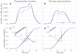
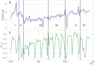
Figure 28: Changes in circadian rhythms during the lock-down measured by number of calls per hour. (A) Network traffic on the last Thursday in phase I, March 4^th. The horizontal arrow marks the full-width-quarter-maximum length (FWQM). (B) Calls per hour on Thursday, March 18^th, the first Thursday in phase III. (C) Normalized cumulative activity for the day shown in panel A. The inset highlights the difference of the male and female curve. The grey shaded area marks the difference between the circadian rhythm of men and women, denoted $\Delta_{FM}$. (D) Same as in C, but for the curve in panel B. (E) FWQM for men and women over time. (F) The gender ratio $r_{FWQM}$ does not deviate strongly from equality, hence, we show $\Delta_{FM}$ over time. For both genders the activity maximum shifts from late afternoon to morning and the length of the activity period is approximately 60 min shorter during the lock-down. The reduction in $\Delta_{FM}$ indicates that the circadian rhythms of men and women become more synchronized.

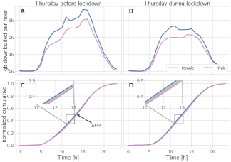
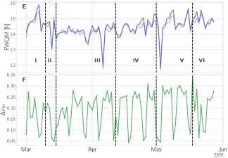
Figure 29: Changes in circadian rhythms during the lock-down measured by downloaded gigabytes per hour. (A) Network traffic on the last Thursday in phase I, March 4^th. The horizontal arrow marks the full-width-quarter-maximum length (FWQM). (B) Downloaded gigabytes per hour on Thursday, March 18^th, the first Thursday in phase III. (C) Normalized cumulative activity for the day shown in panel A. The inset highlights the difference of the male and female curve. The grey shaded area marks the difference between the circadian rhythm of men and women, denoted $\Delta_{FM}$. (D) Same as in C, but for the curve in panel B. (E) FWQM for men and women over time. (F) As $r_{FWQM}$ does not deviate strongly from equality, we display $\Delta_{FM}$ over time. For both genders the activity maximum in the late afternoon disappears and the length of the activity period is approximately 40 min shorter during the lock-down. A slight reduction in $\Delta_{FM}$ indicates that the circadian rhythms of men and women become more synchronized.

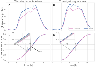
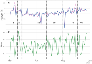
Figure 30: Changes in circadian rhythms during the lock-down measured by uploaded gigabyte per hour. (A) Network traffic on the last Thursday in phase I, March 4^th. The horizontal arrow marks the full-width-quarter-maximum length (FWQM). (B) Uploaded gigabytes per hour on Thursday, March 18^th, the first Thursday in phase III. (C) Normalized cumulative activity for the day shown in panel A. The inset highlights the difference of the male and female curve. The grey shaded area marks the difference between the circadian rhythm of men and women, denoted $\Delta_{FM}$. (D) Same as in C, but for the curve in panel B. (E) FWQM for men and women over time. (F) As $r_{FWQM}$ does not change much from one, we show $\Delta_{FM}$ over time. For both genders the activity maximum shifts from late afternoon to morning and the length of the activity period is approximately 45 min shorter during the lock-down. The reduction in $\Delta_{FM}$ indicates that the circadian rhythms of men and women become more synchronized.

References

- (1) V Palchykov, K Kaski, J Kertész, AL Barabási, RI Dunbar, Sex differences in intimate relationships. Scientific Reports 2, 1–5 (2012).
- (2) L Gauvin, et al., Gender gaps in urban mobility. Humanities and Social Sciences Communications 7, 1–13 (2020).
- (3) DF Halpern, Sex Differences in Cognitive Abilities. (Psychology press), (2013).
- (4) H Ben-Zur, M Zeidner, Gender differences in coping reactions under community crisis and daily routine conditions. Personality and Individual Differences 20, 331–340 (1996).
- (5) MP Matud, Gender differences in stress and coping styles. Personality and Individual Differences 37, 1401–1415 (2004).
- (6) JF Duffy, et al., Sex difference in the near-24-hour intrinsic period of the human circadian timing system. Proceedings of the National Academy of Sciences 108, 15602–15608 (2011).
- (7) A Chmiel, P Klimek, S Thurner, Spreading of diseases through comorbidity networks across life and gender. New Journal of Physics 16, 115013 (2014).
- (8) M Szell, S Thurner, How women organize social networks different from men: gender-specific behavior in large-scale social networks. Scientific Reports 3, 1214 (2013).
- (9) DJ Watts, A twenty-first century science. Nature 445, 489–489 (2007).
- (10) JP Bagrow, D Wang, AL Barabasi, Collective response of human populations to large-scale emergencies. PLOS ONE 6, 1–8 (2011).
- (11) X Lu, L Bengtsson, P Holme, Predictability of population displacement after the 2010 haiti earthquake. Proceedings of the National Academy of Sciences 109, 11576?11581 (2012).
- (12) Q Wang, JE Taylor, Quantifying human mobility perturbation and resilience in hurricane sandy. PLOS ONE 9, e112608 (2014).
- (13) D Garcia, B Rimé, Collective emotions and social resilience in the digital traces after a terrorist attack. Psychological Science 30, 617–628 (2019).
- (14) CT Butts, M Petrescu-Prahova, BR Cross, Responder communication networks in the world trade center disaster: Implications for modeling of communication within emergency settings. The Journal of Mathematical Sociology 31, 121–147 (2007).
- (15) S Gao, et al., Mobile phone location data reveal the effect and geographic variation of social distancing on the spread of the Covid-19 epidemic. https://arxiv.org/abs/2004.11430 (2020) Accessed 8 October 2020.
- (16) N Oliver, et al., Mobile phone data for informing public health actions across the covid-19 pandemic life cycle. Science Advances 6 (2020).
- (17) K Cohen-Louck, I Levy, Risk perception of a chronic threat of terrorism: Differences based on coping types, gender and exposure. International Journal of Psychology 55, 115–122 (2020).
- (18) SE Taylor, et al., Biobehavioral responses to stress in females: Tend-and-befriend, not fight-or-flight. Psychological Review 107, 411 (2000).
- (19) H Wang, et al., The psychological distress and coping styles in the early stages of the 2019 coronavirus disease (covid-19) epidemic in the general mainland chinese population: A web-based survey. PLOS ONE 15, e0233410 (2020).
- (20) S Galea, et al., Psychological sequelae of the september 11 terrorist attacks in new york city. New England Journal of Medicine 346, 982–987 (2002).
- (21) JS Juul, et al., Gender-specific behavior change following terror attacks. https://arxiv.org/abs/2004.02957 (2020) Accessed 8 October 2020.
- (22) A Desvars-Larrive, et al., A structured open dataset of government interventions in response to Covid-19. Scientific Data 7, 1?9 (2020).
- (23) G Heiler, et al., Country-wide mobility changes observed using mobile phone data during Covid-19 pandemic. http://arxiv.org/abs/2008.10064 (2020) Accessed 8 October 2020.
- (24) Asfinag, Asfinag Verkehrszählung. https://www.asfinag.at/verkehr/verkehrszaehlung/ (Online) (2020) Accessed 8 October 2020.
- (25) Market Institut, Corona definiert Arbeitswelten von Morgen neu. https://www.market.at/market-aktuell/details/corona-definiert-arbeitswelten-von-morgen-neu.html (2020) Accessed 8 October 2020.
- (26) Arbeitsmarktservice Austria, Arbeitsmarktdaten - Berichte und Auswertungen. https://www.ams.at/arbeitsmarktdaten-und-medien/arbeitsmarkt-daten-und-arbeitsmarkt-forschung/berichte-und-auswertungen (2020) Accessed 8 October 2020.
- (27) J Hager, Arbeitsmarkt: 1,3 Millionen in Österreich in Kurzarbeit, 517.221 ohne Job, https://kurier.at/politik/inland/live-die-aktuellen-zahlen-zu-arbeitslosigkeit-und-kurzarbeit/400928603 (Kurier Online) (2020).
- (28) M Pellert, J Lasser, H Metzler, D Garcia, Dashboard of sentiment in Austrian social media during COVID-19. http://arxiv.org/abs/2006.11158 (2020) see also http://www.mpellert.at/covid19_monitor_austria/, accessed 8 October 2020.
- (29) IFES and SORA, Home-Office: Positive Resonanz, aber mehr Stress. https://www.ifes.at/arbeitsklima-index-2020-home-office (2020) Accessed 8 October 2020.
- (30) G Viglione, Are women publishing less during the pandemic? here’s what the data say. Nature 581, 365–366 (2020).
- (31) OECD, Women at the core of fight against Covid-19 crisis. https://www.oecd.org/coronavirus/policy-responses/women-at-the-core-of-the-fight-against-covid-19-crisis-553a8269/ (2020) Accessed 8 October 2020.
- (32) C Bradbury-Jones, L Isham, The pandemic paradox: The consequences of COVID-19 on domestic violence. Journal of Clinical Nursing 29, 2047–2049 (2020).
- (33) J Steiner, C Ebert, The Impact of COVID-19 on Violence against Women and Children in Germany. Preprint: https://www.hfp.tum.de/globalhealth/forschung/covid-19-and-domestic-violence/ (2020) Accessed 8 October 2020.
- (34) M Zeidner, Gender Group Differences in Coping with Chronic Terror: The Israeli Scene. Sex Roles 54, 297–310 (2006).
- (35) J Candia, et al., Uncovering individual and collective human dynamics from mobile phone records. Journal of Physics A: Mathematical and Theoretical 41, 224015 (2008).
- (36) J Prashker, Y Shiftan, P Hershkovitch-Sarusi, Residential choice location, gender and the commute trip to work in Tel Aviv. Journal of Transport Geography 16, 332–341 (2008).
- (37) Statistik Austria, Haushalte, familien und lebensformen. http://www.statistik.at/web_de/statistiken/menschen_und_gesellschaft/bevoelkerung/ haushalte_familien_lebensformen/index.html (2019) Accessed 8 October 2020.
- (38) JP Onnela, et al., Structure and tie strengths in mobile communication networks. Proceedings of the National Academy of Sciences 104, 7332–7336 (2007).
- (39) T Igarashi, J Takai, T Yoshida, Gender differences in social network development via mobile phone text messages: A longitudinal study. Journal of Social and Personal Relationships 22, 691–713 (2005).
- (40) B Prainsack, Solidarity in times of a pandemic: What do people do, and why? In preparation. (2020).
- (41) G Michael, S Anastasios, K Helen, K Catherine, K Christine, Gender differences in experiencing occupational stress: the role of age, education and marital status. Stress and Health: Journal of the International Society for the Investigation of Stress 25, 397–404 (2009).
- (42) MB Stein, JR Walker, DR Forde, Gender differences in susceptibility to posttraumatic stress disorder. Behaviour Research and Therapy 38, 619–628 (2000).
- (43) G Parker, H Brotchie, Gender differences in depression. International Review of Psychiatry 22, 429–436 (2010).
- (44) J Török, Y Murase, HH Jo, J Kertész, K Kaski, What big data tells: sampling the social network by communication channels. Physical Review E 94, 052319 (2016).
- (45) M Betz, L O?Connell, JM Shepard, Gender differences in proclivity for unethical behavior. Journal of Business Ethics 8, 321?324 (1989).
- (46) D Dalton, M Ortegren, Gender differences in ethics research: The importance of controlling for the social desirability response bias. Journal of Business Ethics 103, 73?93 (2011).
- (47) KR Moran, SY Del Valle, A meta-analysis of the association between gender and protective behaviors in response to respiratory epidemics and pandemics. PLOS ONE 11, e0164541 (2016).
- (48) JM Eberl, N Lebernegg, J Partheymüller, S Kritzinger, Die meisten nehmen die Lage ernst. Aber wer sind die Corona-Skeptiker? https://viecer.univie.ac.at/corona-blog/corona-blog-beitraege/blog12/ (2020) Accessed 8 October 2020.
- (49) B Kittel, et al., The Austrian corona panel project: Monitoring individual and societal dynamics amidst the Covid-19 crisis (2020).
- (50) PE Gustafsod, Gender Differences in Risk Perception: Theoretical and methodological Perspectives. Risk Analysis 18, 805–811 (1998).
- (51) JP Byrnes, DC Miller, WD Schafer, Gender differences in risk taking: A meta-analysis. Psychological Bulletin 125, 367 (1999).
- (52) T Aledavood, S Lehmann, J Saramäki, Digital daily cycles of individuals. Frontiers in Physics 3, 73 (2015).
- (53) GSMA, The GSMA COVID-19 Privacy Guidelines. https://www.gsma.com/publicpolicy/ resources/covid-19-privacy-guidelines (2020) Accessed 8 October 2020.
- (54) Uber Technologies, H3: Uber’s Hexagonal Hierarchical Spatial Index. https://eng.uber.com/h3/ (2018) Accessed 8 October 2020.
.