VarGrad: A Low-Variance Gradient Estimator for Variational Inference

Lorenz Richter
Freie Universität Berlin
BTU Cottbus-Senftenberg
dida Datenschmiede GmbH
lorenz.richter@fu-berlin.de Ayman Boustati
University of Warwick
a.boustati@warwick.ac.uk Nikolas Nüsken
Universität Potsdam
nuesken@uni-potsdam.de Francisco J. R. Ruiz
DeepMind
franrruiz@google.com Ömer Deniz Akyildiz
University of Warwick
The Alan Turing Institute
omer.akyildiz@warwick.ac.uk
Equal contribution.
Abstract

We analyse the properties of an unbiased gradient estimator of the evidence lower bound (elbo) for variational inference, based on the score function method with leave-one-out control variates. We show that this gradient estimator can be obtained using a new loss, defined as the variance of the log-ratio between the exact posterior and the variational approximation, which we call the log-variance loss. Under certain conditions, the gradient of the log-variance loss equals the gradient of the (negative) elbo. We show theoretically that this gradient estimator, which we call VarGrad due to its connection to the log-variance loss, exhibits lower variance than the score function method in certain settings, and that the leave-one-out control variate coefficients are close to the optimal ones. We empirically demonstrate that VarGrad offers a favourable variance versus computation trade-off compared to other state-of-the-art estimators on a discrete variational autoencoder (vae).

1 Introduction

Estimating the gradient of the expectation of a function is a problem with applications in many areas of machine learning, ranging from variational inference to reinforcement learning (Mohamed et al., 2019). Different gradient estimators lead to different algorithms; two examples of estimators are the score function gradient (Williams, 1992) and the reparameterisation gradient (Kingma and Welling, 2014; Rezende et al., 2014; Titsias and Lázaro-Gredilla, 2014). Many recent works develop new estimators with different properties (such as their variance); see Section 5 for a review.

We focus on variational inference (VI), where the goal is to approximate the posterior distribution p(z|x)𝑝conditional𝑧𝑥p(z\,|\,x) of a model p(x,z)𝑝𝑥𝑧p(x,z), where x𝑥x denotes the observations and z𝑧z refers to the latent variables of the model (Jordan et al., 1999; Blei et al., 2017). VI approximates the posterior using a parameterised family of distributions qϕ(z)subscript𝑞italic-ϕ𝑧q_{\phi}(z), and finds the parameters ϕitalic-ϕ\phi by minimising the Kullback-Leibler (kl) divergence from qϕ(z)subscript𝑞italic-ϕ𝑧q_{\phi}(z) to p(z|x)𝑝conditional𝑧𝑥p(z\,|\,x), i.e., kl(qϕ(z)||p(z|x))\textrm{{kl}}(q_{\phi}(z)\;||\;p(z\,|\,x)). Since the kl is intractable, VI solves instead an equivalent problem that maximises the evidence lower bound (elbo), given by

elbo(ϕ)=𝔼qϕ[logp(x,z)qϕ(z)].elboitalic-ϕsubscript𝔼subscript𝑞italic-ϕ𝑝𝑥𝑧subscript𝑞italic-ϕ𝑧\textrm{{elbo}}(\phi)=\operatorname{\mathbb{E}}_{q_{\phi}}\left[\log\frac{p(x,z)}{q_{\phi}(z)}\right]. (1)

Thus, VI casts the inference problem as an optimisation problem, which can be solved with stochastic optimisation tools when the elbo is not available in closed form. In particular, VI forms a Monte Carlo estimator of the gradient of the elbo, ϕelbo(ϕ)subscriptitalic-ϕelboitalic-ϕ\nabla_{\phi}\textrm{{elbo}}(\phi).

In this paper, we analyse a multi-sample estimator of the gradient of the elbo. In particular, we focus on an estimator first introduced by Salimans and Knowles (2014) and Kool et al. (2019), which is based on the score function method (Williams, 1992) with leave-one-out control variates.

We first show the connection between this estimator and an alternative divergence measure between the variational distribution qϕ(z)subscript𝑞italic-ϕ𝑧q_{\phi}(z) and the exact posterior p(z|x)𝑝conditional𝑧𝑥p(z\,|\,x). This divergence, which is different from the standard kl used in variational inference, is defined as the variance, under some arbitrary distribution r(z)𝑟𝑧r(z), of the log-ratio logqϕ(z)p(z|x)subscript𝑞italic-ϕ𝑧𝑝conditional𝑧𝑥\log\frac{q_{\phi}(z)}{p(z\,|\,x)}. We refer to this divergence as the log-variance loss. Inspired by Nüsken and Richter (2020), we show that we recover the gradient estimator of Salimans and Knowles (2014) and Kool et al. (2019) by taking the gradient with respect to the variational parameters ϕitalic-ϕ\phi of the log-variance loss and evaluating the result at r(z)=qϕ(z)𝑟𝑧subscript𝑞italic-ϕ𝑧r(z)=q_{\phi}(z). Due to this property, we refer to the gradient estimator as VarGrad. This property also suggests a simple algorithm for computing the gradient estimator, based on differentiating through the log-variance loss.

We then study the relationship between VarGrad and the score function estimator (Williams, 1992; Carbonetto et al., 2009; Paisley et al., 2012; Ranganath et al., 2014) with optimal control variate coefficients. We show that the control variate coefficients of VarGrad are close to the (intractable) optimal coefficients. Indeed, we show both theoretically and empirically that the difference between both is small in many cases; for example when the kl from qϕ(z)subscript𝑞italic-ϕ𝑧q_{\phi}(z) to the posterior is either small or large, which is generally the case in the late and early stages of the optimisation, respectively. This explains the success of the VarGrad estimator in a variety of settings (Kool et al., 2019, 2020).

Since it is based on the score function, VarGrad is a black-box, general purpose estimator because it makes no assumptions on the model p(x,z)𝑝𝑥𝑧p(x,z), such as differentiability with respect to the latent variables z𝑧z. It introduces no additional parameters to be tuned and it is not computationally expensive. In Section 6, we show empirically that VarGrad exhibits a favourable variance versus computation trade-off compared to other unbiased gradient estimators, including the score function gradient with control variates (Williams, 1992; Ranganath et al., 2014), rebar (Tucker et al., 2017), relax (Grathwohl et al., 2018), and arm (Yin and Zhou, 2019).

2 Background

In this section, we introduce the notation and review one of the most relevant estimators in VI: the score function method. We also review its improved version based on leave-one-out control variates.

Consider a probabilistic model p(x,z)𝑝𝑥𝑧p(x,z), where z𝑧z denotes the latent variables and x𝑥x are the observations. We are interested in computing the posterior p(z|x)=p(x,z)/p(x)𝑝conditional𝑧𝑥𝑝𝑥𝑧𝑝𝑥p(z\,|\,x)=p(x,z)/p(x), where p(x)=p(x,z)dz𝑝𝑥𝑝𝑥𝑧differential-d𝑧p(x)=\int p(x,z)\;{\mathrm{d}}z is the marginal likelihood. For most models of interest, the posterior is intractable due to the intractability of the marginal likelihood, and we resort to an approximation.

Variational inference approximates the posterior p(z|x)𝑝conditional𝑧𝑥p(z\,|\,x) with a parameterised family of distributions qϕ(z)subscript𝑞italic-ϕ𝑧q_{\phi}(z) (with ϕΦitalic-ϕΦ\phi\in\Phi), called variational family. Variational inference finds the parameters ϕsuperscriptitalic-ϕ\phi^{*} that minimise the kl divergence, ϕ=argminϕΦkl(qϕ(z)||p(z|x))\phi^{*}=\operatornamewithlimits{argmin}_{\phi\in\Phi}\textrm{{kl}}\left(q_{\phi}(z)\;||\;p(z\,|\,x)\right). This optimisation problem is intractable because the kl itself depends on the intractable posterior. Variational inference sidesteps this problem by maximising instead the elbo defined in Eq. 1, which is a lower bound on the marginal likelihood, since logp(x)=elbo(ϕ)+kl(qϕ(z)||p(z|x))\log p(x)=\textrm{{elbo}}(\phi)+\textrm{{kl}}\left(q_{\phi}(z)\;||\;p(z\,|\,x)\right). As the expectation in Eq. 1 is typically intractable, variational inference uses stochastic optimisation to maximise the elbo. In particular, it forms unbiased Monte Carlo estimators of the gradient ϕelbo(ϕ)subscriptitalic-ϕelboitalic-ϕ\nabla_{\phi}\textrm{{elbo}}(\phi).

We next review the score function method, a Monte Carlo estimator commonly used in variational inference. Instead of the elbo, we focus on the gradients of the kl divergence with respect to the variational parameters ϕitalic-ϕ\phi. These gradients are equal to the gradients of the negative elbo because the marginal likelihood p(x)𝑝𝑥p(x) does not depend on ϕitalic-ϕ\phi; that is, ϕkl(qϕ(z)||p(z|x))=ϕelbo(ϕ)\nabla_{\phi}\textrm{{kl}}\left(q_{\phi}(z)\;||\;p(z\,|\,x)\right)=-\nabla_{\phi}\textrm{{elbo}}(\phi).

The score function estimator (Williams, 1992; Carbonetto et al., 2009; Paisley et al., 2012; Ranganath et al., 2014), also known as Reinforce, expresses the gradient as an expectation that depends on the log-ratio qϕ(z)/p(x,z)subscript𝑞italic-ϕ𝑧𝑝𝑥𝑧{q_{\phi}(z)}/{p(x,z)} weighted by the score function ϕlogqϕ(z)subscriptitalic-ϕsubscript𝑞italic-ϕ𝑧\nabla_{\phi}\log q_{\phi}(z). The resulting estimator is

ϕkl[qϕ(z)||p(z|x)]g^Reinforce(ϕ)=1Ss=1Slog(qϕ(z(s))p(x,z(s)))ϕlogqϕ(z(s)),\nabla_{\phi}\textrm{{kl}}\left[q_{\phi}(z)\;||\;p(z\,|\,x)\right]\approx\widehat{g}_{\text{Reinforce}}(\phi)=\frac{1}{S}\sum_{s=1}^{S}\log\!\left(\frac{q_{\phi}(z^{(s)})}{p(x,z^{(s)})}\right)\!\nabla_{\phi}\log q_{\phi}(z^{(s)}), (2)

where z(s)i.i.d.qϕ(z)superscript𝑧𝑠i.i.d.similar-tosubscript𝑞italic-ϕ𝑧z^{(s)}\overset{\textrm{i.i.d.}}{\sim}q_{\phi}(z). Due to its high variance, the score function estimator requires additional tricks in practice; Ranganath et al. (2014) use Rao-Blackwellization and control variates. The control variates are multiples of the score function, aϕlogqϕ(z)direct-product𝑎subscriptitalic-ϕsubscript𝑞italic-ϕ𝑧a\odot\nabla_{\phi}\log q_{\phi}(z), where direct-product\odot denotes the Hadamard (element-wise) product and the coefficient a𝑎a is chosen to minimise the estimator variance.

Salimans and Knowles (2014) and Kool et al. (2019) leverage the multi-sample estimator by using S1𝑆1S-1 samples to compute the control variate coefficient a𝑎a and then average over the resulting estimators, obtaining a leave-one-out estimator

g^LOO(ϕ)=1S1(s=1Sfϕ(z(s))ϕlogqϕ(z(s))f¯ϕs=1Sϕlogqϕ(z(s))),z(s)i.i.d.qϕ(z),subscript^𝑔LOOitalic-ϕ1𝑆1superscriptsubscript𝑠1𝑆subscript𝑓italic-ϕsuperscript𝑧𝑠subscriptitalic-ϕsubscript𝑞italic-ϕsuperscript𝑧𝑠subscript¯𝑓italic-ϕsuperscriptsubscript𝑠1𝑆subscriptitalic-ϕsubscript𝑞italic-ϕsuperscript𝑧𝑠superscript𝑧𝑠i.i.d.similar-tosubscript𝑞italic-ϕ𝑧\displaystyle\widehat{g}_{\text{LOO}}(\phi)=\frac{1}{S-1}\!\!\left(\sum_{s=1}^{S}f_{\phi}(z^{(s)})\nabla_{\phi}\log q_{\phi}(z^{(s)})-\bar{f}_{\phi}\sum_{s=1}^{S}\nabla_{\phi}\log q_{\phi}(z^{(s)})\!\right)\!\!,\quad z^{(s)}\overset{\textrm{i.i.d.}}{\sim}q_{\phi}(z), (3)

where for simplicity of notation we have defined fϕ(z)subscript𝑓italic-ϕ𝑧f_{\phi}(z) as the log-ratio logqϕ(z)p(x,z)subscript𝑞italic-ϕ𝑧𝑝𝑥𝑧\log\frac{q_{\phi}(z)}{p(x,z)} and f¯ϕsubscript¯𝑓italic-ϕ\bar{f}_{\phi} as its empirical average (which is a multi-sample Monte Carlo estimate of the negative elbo), i.e.,

fϕ(z)=logqϕ(z)p(x,z)andf¯ϕ=1Ss=1Sfϕ(z(s))elbo(ϕ).formulae-sequencesubscript𝑓italic-ϕ𝑧subscript𝑞italic-ϕ𝑧𝑝𝑥𝑧andsubscript¯𝑓italic-ϕ1𝑆superscriptsubscript𝑠1𝑆subscript𝑓italic-ϕsuperscript𝑧𝑠elboitalic-ϕf_{\phi}(z)=\log\frac{q_{\phi}(z)}{p(x,z)}\quad\textrm{and}\quad\bar{f}_{\phi}=\frac{1}{S}\sum_{s=1}^{S}f_{\phi}(z^{(s)})\approx-\textrm{{elbo}}(\phi). (4)

The score function method makes no assumptions on the model p(x,z)𝑝𝑥𝑧p(x,z) or the distribution qϕ(z)subscript𝑞italic-ϕ𝑧q_{\phi}(z); the only requirements are to be able to sample from qϕ(z)subscript𝑞italic-ϕ𝑧q_{\phi}(z) and to evaluate logqϕ(z)subscript𝑞italic-ϕ𝑧\log q_{\phi}(z) and logp(x,z)𝑝𝑥𝑧\log p(x,z).

3 The Log-Variance Loss and its Connection to VarGrad

In this section, we show the connection between the leave-one-out estimator in Eq. 3 and a novel divergence, which we call the log-variance loss. We introduce the log-variance loss in Section 3.1 and show its connection to Eq. 3 in Section 3.2. We refer to the estimator in Eq. 3 as VarGrad.

3.1 The Log-Variance Loss

The log-variance loss is defined as the variance, under some arbitrary distribution r(z)𝑟𝑧r(z), of the log-ratio logqϕ(z)p(z|x)subscript𝑞italic-ϕ𝑧𝑝conditional𝑧𝑥\log\frac{q_{\phi}(z)}{p(z\,|\,x)}. It has the property of reproducing the gradients of the kl divergence under certain conditions (see Proposition 1 for details). We next give the precise definition of the loss.

Definition 1.

For a given distribution r(z)𝑟𝑧r(z), the log-variance loss r()subscript𝑟\mathcal{L}_{r}(\cdot) is given by

r(qϕ(z)||p(z|x))\displaystyle\mathcal{L}_{r}(q_{\phi}(z)\;||\;p(z\,|\,x)) =12Varr(log(qϕ(z)p(z|x))).absent12subscriptVar𝑟subscript𝑞italic-ϕ𝑧𝑝conditional𝑧𝑥\displaystyle=\frac{1}{2}\textnormal{Var}_{r}\left(\log\left(\frac{q_{\phi}(z)}{p(z\,|\,x)}\right)\right). (5)

We refer to the distribution r(z)𝑟𝑧r(z) as the reference distribution under which the discrepancy between qϕ(z)subscript𝑞italic-ϕ𝑧q_{\phi}(z) and the posterior p(z|x)𝑝conditional𝑧𝑥p(z\,|\,x) is computed. When the support of the reference distribution contains the supports of qϕ(z)subscript𝑞italic-ϕ𝑧q_{\phi}(z) and p(z|x)𝑝conditional𝑧𝑥p(z\,|\,x), Eq. 5 is a divergence;***More technically, as we assume that r(z)𝑟𝑧r(z), p(z|x)𝑝conditional𝑧𝑥p(z\,|\,x), and qϕ(z)subscript𝑞italic-ϕ𝑧q_{\phi}(z) admit densities, it follows that measure-zero sets of r(z)𝑟𝑧r(z) are necessarily measure-zero sets of p(z|x)𝑝conditional𝑧𝑥p(z\,|\,x) and qϕ(z)subscript𝑞italic-ϕ𝑧q_{\phi}(z), implying that the divergence is well defined. it is zero if and only if qϕ(z)=p(z|x)subscript𝑞italic-ϕ𝑧𝑝conditional𝑧𝑥q_{\phi}(z)=p(z\,|\,x). The factor 1/2121/2 in Eq. 5 is only included because it simplifies some expressions later in this section.

We next show that the gradient of the log-variance loss and the gradient of the standard kl divergence coincide under certain conditions. In particular, taking the gradient of Eq. 5 with respect to the variational parameters ϕitalic-ϕ\phi and then evaluating the result for a reference distribution r(z)=qϕ(z)𝑟𝑧subscript𝑞italic-ϕ𝑧r(z)=q_{\phi}(z) gives the gradient of the kl. This property is detailed in Proposition 1.

Proposition 1.

The gradient with respect to ϕitalic-ϕ\phi of the log-variance loss, evaluated at r(z)=qϕ(z)𝑟𝑧subscript𝑞italic-ϕ𝑧r(z)=q_{\phi}(z), equals the gradient of the kl divergence,

ϕr(qϕ(z)||p(z|x))|r=qϕ=ϕkl(qϕ(z)||p(z|x)).\nabla_{\phi}\mathcal{L}_{r}(q_{\phi}(z)\;||\;p(z\,|\,x))\Big{|}_{r=q_{\phi}}=\nabla_{\phi}\textrm{{kl}}(q_{\phi}(z)\;||\;p(z\,|\,x)). (6)
Proof.

See Section A.1. \Box

Proposition 1 implies that we can estimate the gradient of the kl divergence by estimating instead the gradient of the log-variance loss.

Remark 1.

The result in Proposition 1 is obtained by setting r(z)=qϕ(z)𝑟𝑧subscript𝑞italic-ϕ𝑧r(z)=q_{\phi}(z) after taking the gradient with respect to ϕitalic-ϕ\phi. The same result does not hold if we set r(z)=qϕ(z)𝑟𝑧subscript𝑞italic-ϕ𝑧r(z)=q_{\phi}(z) before differentiating.

3.2 VarGrad: Derivation of the Gradient Estimator from the Log-Variance Loss

The leave-one-out estimator in Eq. 3 (Salimans and Knowles, 2014; Kool et al., 2019) is connected to the log-variance loss from Section 3.1 through Proposition 1. Firstly, note that the log-variance loss is intractable as it depends on the posterior p(z|x)𝑝conditional𝑧𝑥p(z\,|\,x). However, since the marginal likelihood p(x)𝑝𝑥p(x) has zero variance, it can be dropped from the definition in Eq. 5, yielding

r(qϕ(z)||p(z|x))=12Varr(log(qϕ(z)p(x,z)))=12Varr(fϕ(z)),\mathcal{L}_{r}(q_{\phi}(z)\;||\;p(z\,|\,x))=\frac{1}{2}\text{Var}_{r}\left(\log\left(\frac{q_{\phi}(z)}{p(x,z)}\right)\right)=\frac{1}{2}\text{Var}_{r}\left(f_{\phi}(z)\right), (7)

where fϕ(z)subscript𝑓italic-ϕ𝑧f_{\phi}(z) is defined in Eq. 4.

Next, we build the estimator of the log-variance loss as the empirical variance of S𝑆S Monte Carlo samples,

r(qϕ(z)||p(z|x))12(S1)s=1S(fϕ(z(s))f¯ϕ)2,z(s)i.i.d.r(z).\mathcal{L}_{r}(q_{\phi}(z)\;||\;p(z\,|\,x))\approx\frac{1}{2(S-1)}\sum_{s=1}^{S}\left(f_{\phi}(z^{(s)})-\bar{f}_{\phi}\right)^{2},\quad z^{(s)}\overset{\textrm{i.i.d.}}{\sim}r(z). (8)

Applying Proposition 1 by differentiating through Eq. 8, we arrive at the VarGrad estimator, g^VarGrad(ϕ)=g^LOO(ϕ)ϕkl(qϕ(z)||p(z|x))\widehat{g}_{\text{VarGrad}}(\phi)=\widehat{g}_{\text{LOO}}(\phi)\approx\nabla_{\phi}\textrm{{kl}}\left(q_{\phi}(z)\;||\;p(z\,|\,x)\right), where

g^VarGrad(ϕ)=1S1(s=1Sfϕ(z(s))ϕlogqϕ(z(s))f¯ϕs=1Sϕlogqϕ(z(s)))subscript^𝑔VarGraditalic-ϕ1𝑆1superscriptsubscript𝑠1𝑆subscript𝑓italic-ϕsuperscript𝑧𝑠subscriptitalic-ϕsubscript𝑞italic-ϕsuperscript𝑧𝑠subscript¯𝑓italic-ϕsuperscriptsubscript𝑠1𝑆subscriptitalic-ϕsubscript𝑞italic-ϕsuperscript𝑧𝑠\displaystyle\widehat{g}_{\text{VarGrad}}(\phi)=\frac{1}{S-1}\!\!\left(\sum_{s=1}^{S}f_{\phi}(z^{(s)})\nabla_{\phi}\log q_{\phi}(z^{(s)})-\bar{f}_{\phi}\sum_{s=1}^{S}\nabla_{\phi}\log q_{\phi}(z^{(s)})\!\right)\!\! (9)

and z(s)i.i.d.qϕ(z)superscript𝑧𝑠i.i.d.similar-tosubscript𝑞italic-ϕ𝑧z^{(s)}\overset{\textrm{i.i.d.}}{\sim}q_{\phi}(z).

The expression for VarGrad in Eq. 9 is identical to that of the leave-one-out estimator in Eq. 3. Thus, VarGrad is an unbiased estimator of the gradient of the kl (and equivalently the gradient of the elbo). From a probabilistic programming perspective, setting the reference r(z)=qϕ(z)𝑟𝑧subscript𝑞italic-ϕ𝑧r(z)=q_{\phi}(z) after differentiating w.r.t. ϕitalic-ϕ\phi amounts to sampling z(s)qϕ(z)similar-tosuperscript𝑧𝑠subscript𝑞italic-ϕ𝑧z^{(s)}\sim q_{\phi}(z) and detaching the resulting samples from the computational graph. This suggests a novel algorithmic procedure, given in Algorithm 1. Its implementation is simple: we only need the samples z(s)qϕ(z)similar-tosuperscript𝑧𝑠subscript𝑞italic-ϕ𝑧z^{(s)}\sim q_{\phi}(z) and apply the stop_gradient operator, evaluate the log-ratio fϕ(z(s))subscript𝑓italic-ϕsuperscript𝑧𝑠f_{\phi}(z^{(s)}) for each sample, and then differentiate through the empirical variance of this log-ratio.

Algorithm 1 Pseudocode for VarGrad
Variational parameters ϕitalic-ϕ\phi, data x𝑥x
for s=1,,S𝑠1𝑆s=1,\ldots,S do
     z(s)𝚜𝚊𝚖𝚙𝚕𝚎(qϕ())superscript𝑧𝑠𝚜𝚊𝚖𝚙𝚕𝚎subscript𝑞italic-ϕz^{(s)}\leftarrow\verb+sample+(q_{\phi}(\cdot)) \triangleright Sample from the approximate posterior
     z(s)stop_gradient(z(s))superscript𝑧𝑠monospace-stop_gradientsuperscript𝑧𝑠z^{(s)}\leftarrow\verb+stop_gradient+(z^{(s)}) \triangleright Detach the samples from the computational graph
     fϕ(s)logqϕ(z(s))logp(x,z(s))superscriptsubscript𝑓italic-ϕ𝑠subscript𝑞italic-ϕsuperscript𝑧𝑠𝑝𝑥superscript𝑧𝑠f_{\phi}^{(s)}\leftarrow\log q_{\phi}(z^{(s)})-\log p(x,z^{(s)}) \triangleright An estimate of the negative elbo
^^absent\widehat{\mathcal{L}}\leftarrow 12𝚅𝚊𝚛𝚒𝚊𝚗𝚌𝚎({fϕ(s)}s=1S\frac{1}{2}\verb+Variance+(\{f_{\phi}^{(s)}\}_{s=1}^{S}) \triangleright An estimate of the log-variance loss
return grad(^)^(\widehat{\mathcal{L}}) \triangleright Differentiate through the loss w.r.t. ϕitalic-ϕ\phi

4 Analytical Results

In this section we study the properties of g^VarGradsubscript^𝑔VarGrad\widehat{g}_{\text{VarGrad}} in comparison to other estimators based on the score function method. In Section 4.1, we analyse the difference δCVsuperscript𝛿CV\delta^{\text{CV}} between the control variate coefficient of VarGrad (called aVarGradsuperscript𝑎VarGrada^{\text{VarGrad}}) and the optimal one. The former can be approximated cheaply and unbiasedly, while a standard Monte Carlo estimator of the latter is biased and often exhibits high variance. Furthermore, we establish that the difference δCVsuperscript𝛿CV\delta^{\text{CV}} is negligible in certain settings, in particular when kl(qϕ(z)||p(z|x))\textrm{{kl}}(q_{\phi}(z)\;||\;p(z\,|\,x)) is either very large or close to zero; thus in these settings the control variate coefficient of VarGrad is close to the optimal coefficient. In Section 4.2 we show that a simple relation between δCVsuperscript𝛿CV\delta^{\text{CV}} and the elbo is sufficient to guarantee that g^VarGradsubscript^𝑔VarGrad\widehat{g}_{\text{VarGrad}} has lower variance than g^Reinforcesubscript^𝑔Reinforce\widehat{g}_{\text{Reinforce}} when the number of Monte Carlo samples is large enough.

4.1 Analysis of the Control Variate Coefficients

As alluded to in Section 2, Ranganath et al. (2014) proposed to modify g^Reinforcesubscript^𝑔Reinforce\widehat{g}_{\text{Reinforce}} using a score function control variate, that is,

g^CV(ϕ)=g^Reinforce(ϕ)a(1Ss=1Sϕlogqϕ(z(s))),subscript^𝑔CVitalic-ϕsubscript^𝑔Reinforceitalic-ϕdirect-product𝑎1𝑆superscriptsubscript𝑠1𝑆subscriptitalic-ϕsubscript𝑞italic-ϕsuperscript𝑧𝑠\widehat{g}_{\text{CV}}(\phi)=\widehat{g}_{\text{Reinforce}}(\phi)-a\odot\left(\frac{1}{S}\sum_{s=1}^{S}\nabla_{\phi}\log q_{\phi}(z^{(s)})\right), (10)

where a𝑎a is a vector chosen so as to reduce the variance of the estimator. We recover VarGrad (Eq. 9), up to a factor of proportionality, by setting the control variate coefficient a=f¯ϕ𝟏𝑎subscript¯𝑓italic-ϕ1a=\bar{f}_{\phi}\mathbf{1} in Eq. 10, where 𝟏1\mathbf{1} is a vector of ones. The proportionality relation is S1Sg^CV=g^VarGrad𝑆1𝑆subscript^𝑔CVsubscript^𝑔VarGrad\frac{S-1}{S}\widehat{g}_{\text{CV}}=\widehat{g}_{\text{VarGrad}}. In terms of variance reduction, the coefficients of the optimal asuperscript𝑎a^{*} are given by

ai=Covqϕ(fϕϕilogqϕ,ϕilogqϕ)Varqϕ(ϕilogqϕ).superscriptsubscript𝑎𝑖subscriptCovsubscript𝑞italic-ϕsubscript𝑓italic-ϕsubscriptsubscriptitalic-ϕ𝑖subscript𝑞italic-ϕsubscriptsubscriptitalic-ϕ𝑖subscript𝑞italic-ϕsubscriptVarsubscript𝑞italic-ϕsubscriptsubscriptitalic-ϕ𝑖subscript𝑞italic-ϕa_{i}^{*}=\frac{\operatorname{Cov}_{q_{\phi}}\left(f_{\phi}\partial_{\phi_{i}}\log q_{\phi},\partial_{\phi_{i}}\log q_{\phi}\right)}{\operatorname{Var}_{q_{\phi}}\left(\partial_{\phi_{i}}\log q_{\phi}\right)}. (11)

We next show that the coefficients of VarGrad, aVarGradsuperscript𝑎VarGrada^{\text{VarGrad}}, are close to the optimal coefficients asuperscript𝑎a^{*}. For this, we first relate aVarGradsuperscript𝑎VarGrada^{\text{VarGrad}} to asuperscript𝑎a^{*} in Lemma 1.

Lemma 1.

We can write the optimal control variate coefficient as the expected value of aVarGradsuperscript𝑎VarGrada^{\text{VarGrad}} plus a control variate correction term δCVsuperscript𝛿CV\delta^{\text{CV}}, i.e.,

a=𝔼qϕ[aVarGrad]+δCV=ELBO(ϕ)+δCV,superscript𝑎subscript𝔼subscript𝑞italic-ϕdelimited-[]superscript𝑎VarGradsuperscript𝛿CVELBOitalic-ϕsuperscript𝛿CVa^{*}=\mathbb{E}_{q_{\phi}}[a^{\text{VarGrad}}]+\delta^{\text{CV}}=-\mathrm{ELBO}(\phi)+\delta^{\text{CV}}, (12)

where aVarGrad=f¯ϕsuperscript𝑎VarGradsubscript¯𝑓italic-ϕa^{\text{VarGrad}}=\bar{f}_{\phi} and the components of the correction term δCVsuperscript𝛿CV\delta^{\text{CV}} are given by

δiCV=Covqϕ(fϕ,(ϕilogqϕ)2)Varqϕ(ϕilogqϕ).subscriptsuperscript𝛿CV𝑖subscriptCovsubscript𝑞italic-ϕsubscript𝑓italic-ϕsuperscriptsubscriptsubscriptitalic-ϕ𝑖subscript𝑞italic-ϕ2subscriptVarsubscript𝑞italic-ϕsubscriptsubscriptitalic-ϕ𝑖subscript𝑞italic-ϕ\delta^{\text{CV}}_{i}=\frac{\operatorname{Cov}_{q_{\phi}}\left(f_{\phi},\left(\partial_{\phi_{i}}\log q_{\phi}\right)^{2}\right)}{\operatorname{Var}_{q_{\phi}}\left(\partial_{\phi_{i}}\log q_{\phi}\right)}. (13)
Proof.

See Section A.2. \Box

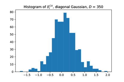
According to Lemma 1, the difference between the optimal control variate coefficient and the (expected) VarGrad coefficient is equal to the correction δCVsuperscript𝛿CV\delta^{\text{CV}}. We hypothesise that direct Monte Carlo estimation of δCVsuperscript𝛿CV\delta^{\text{CV}} in Eq. 13 (or similarly for Eq. 11) suffers from high variance because it takes the form of a fraction Monte Carlo estimators of fractions are not straightforward. As a simple example, consider the ratio of two independent Gaussian random variables, each with zero mean and unit variance. The ratio follows a Cauchy distribution, which has infinite variance. (see for instance Appendix C). Moreover, estimating Eq. 13 by taking the ratio of two Monte Carlo estimators gives a biased estimate.

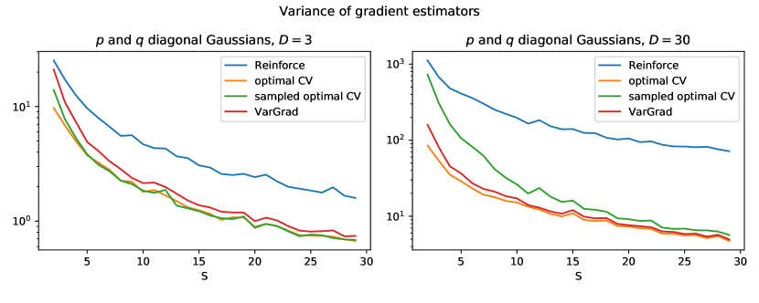
We next show that in certain settings the correction term δCVsuperscript𝛿CV\delta^{\text{CV}} becomes negligible, implying that g^VarGradsubscript^𝑔VarGrad\widehat{g}_{\text{VarGrad}} and g^Reinforcesubscript^𝑔Reinforce\widehat{g}_{\text{Reinforce}} equipped with the optimal control variate coefficients behave almost identically. We provide empirical evidence of this finding in Section 6 (and in Appendix C for the Gaussian case).

Proposition 2 (δCVsuperscript𝛿CV\delta^{\text{CV}} is small in comparison to 𝔼qϕ[aVarGrad]subscript𝔼subscript𝑞italic-ϕdelimited-[]superscript𝑎VarGrad\mathbb{E}_{q_{\phi}}[a^{\text{VarGrad}}{]} if the kl divergence between qϕ(z)subscript𝑞italic-ϕ𝑧q_{\phi}(z) and p(z|x)𝑝conditional𝑧𝑥p(z\,|\,x) is large or small).

Assume that qϕ(z)subscript𝑞italic-ϕ𝑧q_{\phi}(z) has lighter tails than the posterior p(z|x)𝑝conditional𝑧𝑥p(z\,|\,x), in the sense that there exists a constant C>0𝐶0C>0 such that

supzqϕ(z)p(z|x)<C.subscriptsupremum𝑧subscript𝑞italic-ϕ𝑧𝑝conditional𝑧𝑥𝐶\sup_{z}\frac{q_{\phi}(z)}{p(z\,|\,x)}<C. (14)

Furthermore, define the kurtosis of the score function,

Kurt[ϕilogqϕ]=𝔼qϕ[(ϕilogqϕ)4](𝔼qϕ[(ϕilogqϕ)2])2,Kurtdelimited-[]subscriptsubscriptitalic-ϕ𝑖subscript𝑞italic-ϕsubscript𝔼subscript𝑞italic-ϕdelimited-[]superscriptsubscriptsubscriptitalic-ϕ𝑖subscript𝑞italic-ϕ4superscriptsubscript𝔼subscript𝑞italic-ϕdelimited-[]superscriptsubscriptsubscriptitalic-ϕ𝑖subscript𝑞italic-ϕ22\mathrm{Kurt}[\partial_{\phi_{i}}\log q_{\phi}]=\frac{\mathbb{E}_{q_{\phi}}[(\partial_{\phi_{i}}\log q_{\phi})^{4}]}{(\mathbb{E}_{q_{\phi}}[(\partial_{\phi_{i}}\log q_{\phi})^{2}])^{2}}, (15)

and assume that it is bounded, Kurt[ϕilogqϕ]<Kurtdelimited-[]subscriptsubscriptitalic-ϕ𝑖subscript𝑞italic-ϕ\mathrm{Kurt}[\partial_{\phi_{i}}\log q_{\phi}]<\infty. Then, the ratio between the control variate correction δCVsuperscript𝛿CV\delta^{\text{CV}} and the expected control variate coefficient of VarGrad can be upper bounded by

|δiCV𝔼qϕ[aVarGrad]|2CKurt[ϕilogqϕ]|kl(qϕ(z)||p(z|x))logp(x)kl(qϕ(z)||p(z|x))|.\left|\frac{\delta^{\text{CV}}_{i}}{\mathbb{E}_{q_{\phi}}[a^{\text{VarGrad}}]}\right|\leq\frac{2\sqrt{C\,\mathrm{Kurt}[\partial_{\phi_{i}}\log q_{\phi}]}}{\left|\sqrt{\textrm{{kl}}(q_{\phi}(z)\;||\;p(z\,|\,x))}-\frac{\log p(x)}{\sqrt{\textrm{{kl}}(q_{\phi}(z)\;||\;p(z\,|\,x))}}\right|}. (16)
Proof.

See Section A.3. \Box

Remark 2.

The variational approximation qϕ(z)subscript𝑞italic-ϕ𝑧q_{\phi}(z) typically underestimates the spread of the posterior p(z|x)𝑝conditional𝑧𝑥p(z\,|\,x) (Blei et al., 2017), and so the assumption in Eq. 14 is typically satisfied in practice after a few iterations of the optimisation algorithm. The kurtosis Kurt[ϕilogqϕ]Kurtdelimited-[]subscriptsubscriptitalic-ϕ𝑖subscript𝑞italic-ϕ\mathrm{Kurt}[\partial_{\phi_{i}}\log q_{\phi}] quantifies the weight of the tails of the variational approximation in terms of the score function. In Section A.6 we analyse the kurtosis of exponential family distributions and show that it is uniformly bounded for Gaussian variational families.

Remark 3.

The upper bound in Eq. 16 allows us to identify two regimes. When kl(qϕ(z)||p(z|x))\textrm{{kl}}(q_{\phi}(z)\;||\;p(z\,|\,x)) is large, the bound asserts that the relative error satisfies

|δiCV𝔼qϕ[aVarGrad]|𝒪(kl(qϕ(z)||p(z|x))1/2),\displaystyle\left|\frac{\delta^{\textnormal{CV}}_{i}}{\mathbb{E}_{q_{\phi}}[a^{\text{VarGrad}}]}\right|\lessapprox\mathcal{O}\left(\textrm{{kl}}(q_{\phi}(z)\;||\;p(z\,|\,x))^{-1/2}\right), (17)

as the second term in the denominator of Eq. 16 becomes negligible. This can happen in the early stages of the optimisation process, in which case we can conclude that δCVsuperscript𝛿CV\delta^{\text{CV}} is expected to be small. Since the kl divergence increases with the dimensionality of the latent variable z𝑧z (see Section A.7), Eq. 16 also implies that the ratio becomes smaller as the number of latent variables grows. Moreover, if the minimum kl divergence between the variational family and the true posterior is large (i.e., if the best candidate in the variational family is still far away from the target), the correction term δiCVsuperscriptsubscript𝛿𝑖CV\delta_{i}^{\text{CV}} can be negligible during the whole optimisation procedure, which is often the case in practice.

In the regime where kl(qϕ(z)||p(z|x))\textrm{{kl}}(q_{\phi}(z)\;||\;p(z\,|\,x)) approaches zero (i.e., towards the end of the optimisation process if the variational family is well specified and includes the posterior), then Eq. 16 implies that

|δiCV𝔼qϕ[aVarGrad]|𝒪(kl(qϕ(z)||p(z|x))1/2).\displaystyle\left|\frac{\delta^{\text{CV}}_{i}}{\mathbb{E}_{q_{\phi}}[a^{\text{VarGrad}}]}\right|\lessapprox\mathcal{O}\left(\textrm{{kl}}(q_{\phi}(z)\;||\;p(z\,|\,x))^{1/2}\right). (18)

In this regime, the error w.r.t. the optimal control variate coefficient decreases with the kl divergence. The estimates in Eq. 17 and Eq. 18 combined suggest that the relative error remains bounded throughout the optimisation. We verify this proposition experimentally in Section 6.

4.2 Variance of the Estimator

In this section we provide a result that guarantees that the variance of g^VarGradsubscript^𝑔VarGrad\widehat{g}_{\text{VarGrad}} is smaller than the variance of g^Reinforcesubscript^𝑔Reinforce\widehat{g}_{\text{Reinforce}} when the number of Monte Carlo samples is large enough.

Proposition 3.

Consider the two gradient estimators g^Reinforce(ϕ)subscript^𝑔Reinforceitalic-ϕ\widehat{g}_{\text{Reinforce}}(\phi) and g^VarGrad(ϕ)subscript^𝑔VarGraditalic-ϕ\widehat{g}_{\text{VarGrad}}(\phi), each with S𝑆S Monte Carlo samples, as defined in Eq. 2 and Eq. 9, respectively. If

δiCV𝔼qϕ[aVarGrad]=δiCVELBO(ϕ)<12subscriptsuperscript𝛿CV𝑖subscript𝔼subscript𝑞italic-ϕdelimited-[]superscript𝑎VarGradsubscriptsuperscript𝛿CV𝑖ELBOitalic-ϕ12-\frac{\delta^{\text{CV}}_{i}}{\mathbb{E}_{q_{\phi}}[a^{\text{VarGrad}}]}=\frac{\delta^{\text{CV}}_{i}}{\mathrm{ELBO}(\phi)}<\frac{1}{2} (19)

then there exists S0subscript𝑆0S_{0}\in\mathbb{N} such that

Var(g^VarGrad,i(ϕ))Var(g^Reinforce,i(ϕ)),for allSS0.formulae-sequenceVarsubscript^𝑔VarGrad𝑖italic-ϕVarsubscript^𝑔Reinforce𝑖italic-ϕfor all𝑆subscript𝑆0\operatorname{Var}\left(\widehat{g}_{\text{VarGrad},i}(\phi)\right)\leq\operatorname{Var}\left(\widehat{g}_{\text{Reinforce},i}(\phi)\right),\quad\quad\textnormal{for all}\quad S\geq S_{0}. (20)
Proof.

See Section A.4. \Box

If the correction δCVsuperscript𝛿CV\delta^{\text{CV}} is negligible in the sense of Proposition 2, then the assumption in Eq. 19 is satisfied and Proposition 3 guarantees that VarGrad has lower variance than Reinforce when S𝑆S is large enough. We arrive at the following corollary, which also considers the dimensionality of the latent variables. The main assumption -that the kl-divergence increases with the dimension of the latent space- is supported by the result in Section A.7.

Corollary 1.

Let S𝑆S be the number of samples and D𝐷D the dimension of the latent variable z𝑧z. Furthermore, let the assumptions of Eq. 16 be satisfied and assume that kl(qϕ(z)||p(z|x))\textrm{{kl}}(q_{\phi}(z)\;||\;p(z\,|\,x)) is strictly increasing in D𝐷D. Then, there exist S0,D0subscript𝑆0subscript𝐷0S_{0},D_{0}\in\mathbb{N} such that

Var(g^VarGrad,i(ϕ))Var(g^Reinforce,i(ϕ)),for all SS0 and DD0.formulae-sequenceVarsubscript^𝑔VarGrad𝑖italic-ϕVarsubscript^𝑔Reinforce𝑖italic-ϕfor all 𝑆subscript𝑆0 and 𝐷subscript𝐷0\operatorname{Var}\left(\widehat{g}_{\text{VarGrad},i}(\phi)\right)\leq\operatorname{Var}\left(\widehat{g}_{\text{Reinforce},i}(\phi)\right),\quad\quad\textnormal{for all }S\geq S_{0}\textnormal{ and }D\geq D_{0}. (21)
Proof.

See Section A.5. \Box

We provide further intuition on the condition in Eq. 19 with the analysis in Section C.1.

5 Related Work

In the last few years, many gradient estimators of the elbo have been proposed; see Mohamed et al. (2019) for a comprehensive review. Among those, the score function estimators (Williams, 1992; Carbonetto et al., 2009; Paisley et al., 2012; Ranganath et al., 2014) and the reparameterisation estimators (Kingma and Welling, 2014; Rezende et al., 2014; Titsias and Lázaro-Gredilla, 2014), as well as combinations of both (Ruiz et al., 2016; Naesseth et al., 2017), are arguably the most widely used. nvil (Mnih and Gregor, 2014) and MuProp (Gu et al., 2016) are unbiased gradient estimators for training stochastic neural networks.

Other gradient estimators are specific for discrete-valued latent variables. The concrete relaxation (Maddison et al., 2017; Jang et al., 2017) described a way to form a biased estimator of the gradient, which rebar (Tucker et al., 2017) and relax (Grathwohl et al., 2018) use as a control variate to obtain an unbiased estimator. Other recent estimators have been proposed by Lee et al. (2018); Peters and Welling (2018); Shayer et al. (2018); Cong et al. (2019); Yin and Zhou (2019); Yin et al. (2019), and Dong et al. (2020). In Section 6, we compare VarGrad with some of these estimators, showing that it exhibits a favourable performance versus computational complexity trade-off.

The VarGrad estimator was first introduced by Salimans and Knowles (2014) and Kool et al. (2019). It also relates to vimco (Mnih and Rezende, 2016) in that it is a leave-one-out estimator. In this paper, we have described an alternative derivation of VarGrad, based on the log-variance loss.

The log-variance loss from Section 3.1 defines an alternative divergence between the approximate and the exact posterior distributions. In the context of optimal control of diffusion processes and related forward-backward stochastic differential equations, it arises naturally to quantify the discrepancy between measures on path space (Nüsken and Richter, 2020). Other forms of alternative divergences have also been explored in previous work; for example the χ2superscript𝜒2\chi^{2}-divergence (Dieng et al., 2017), the Rényi divergence (Li and Turner, 2016), the Langevin-Stein (Ranganath et al., 2016), the α𝛼\alpha-divergence (Hernández-Lobato et al., 2016), other f𝑓f-divergences (Wang et al., 2018), a contrastive divergence (Ruiz and Titsias, 2019), and also the inclusive kl (Naesseth et al., 2020), see also Appendix D.

Finally, from an implementation perspective, Algorithm 1 contains a stop_gradient operator that resembles the method of Roeder et al. (2017). In Roeder et al. (2017), this operator is used on the variational parameters to eliminate the entropy term in the reparameterisation gradient to reduce its variance; this has also been extended to importance weighted variational objectives (Tucker et al., 2018). In contrast, VarGrad applies the stop_gradient operator on the samples and is based on the score function method.

6 Experiments
Refer to caption
(a)
Refer to caption
(b)
Refer to caption
(c)
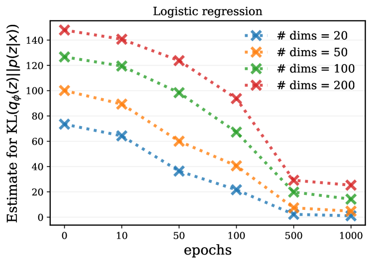
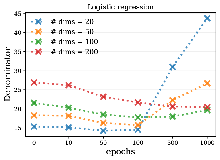
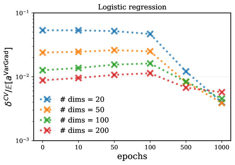
Figure 1: Illustration of Proposition 2 and Remark 3 on the logistic regression model. In (a), we show that the ratio |δiCV/𝔼qϕ[aVarGrad]|subscriptsuperscript𝛿CV𝑖subscript𝔼subscript𝑞italic-ϕdelimited-[]superscript𝑎VarGrad\left|{\delta^{\textnormal{CV}}_{i}}/{\mathbb{E}_{q_{\phi}}[a^{\text{VarGrad}}]}\right| is small and uniformly bounded over epochs, illustrating that the VarGrad estimator stays close to the optimal control variate coefficients during the whole optimisation procedure. Additionally, this ratio decreases with increasing dimensionality of the latent variables. In (b), we display an estimate of the kl divergence across epochs and demonstrate the beneficial effect of higher dimensions, since the bound of Eq. 16 is expected to scale like 𝒪(kl1/2)𝒪superscriptkl12\mathcal{O}(\mathrm{\textsc{kl}}^{-1/2}) in the early phase. In (c), we plot an estimate of the denominator of the bound (Eq. 16), which increases or stays constant over epochs, demonstrating that the ratio in Eq. 16 stays stable (and small) over epochs.
In order to verify the properties of VarGrad empirically, we test it on two popular models: a Bayesian logistic regression model on a synthetic dataset and a discrete variational autoencoder (dvae) (Salakhutdinov and Murray, 2008; Kingma and Welling, 2014) on a fixed binarisation of Omniglot (Lake et al., 2015). All details of the experiments can be found in Appendix B.Code in JAX (Bradbury et al., 2018; Hennigan et al., 2020) is available at https://github.com/aboustati/vargrad.

Closeness to the optimal control variate.  In Section 4 we analytically showed that VarGrad is close to the optimal control variate, and in particular that the ratio |δiCV/𝔼qϕ[aVarGrad]|subscriptsuperscript𝛿CV𝑖subscript𝔼subscript𝑞italic-ϕdelimited-[]superscript𝑎VarGrad\left|{\delta^{\textnormal{CV}}_{i}}/{\mathbb{E}_{q_{\phi}}[a^{\text{VarGrad}}]}\right| can be small over the whole optimisation procedure. This behaviour is expected to be even more pronounced with growing dimensionality of the latent space. In Figure 1, we confirm this result by showing the ratio |δiCV/𝔼qϕ[aVarGrad]|subscriptsuperscript𝛿CV𝑖subscript𝔼subscript𝑞italic-ϕdelimited-[]superscript𝑎VarGrad\left|{\delta^{\textnormal{CV}}_{i}}/{\mathbb{E}_{q_{\phi}}[a^{\text{VarGrad}}]}\right| for the logistic regression model. We also show the kl divergence along the iterations and the denominator of the bound in Eq. 16; see Figure 1 for the details.

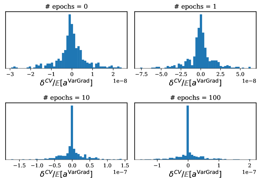
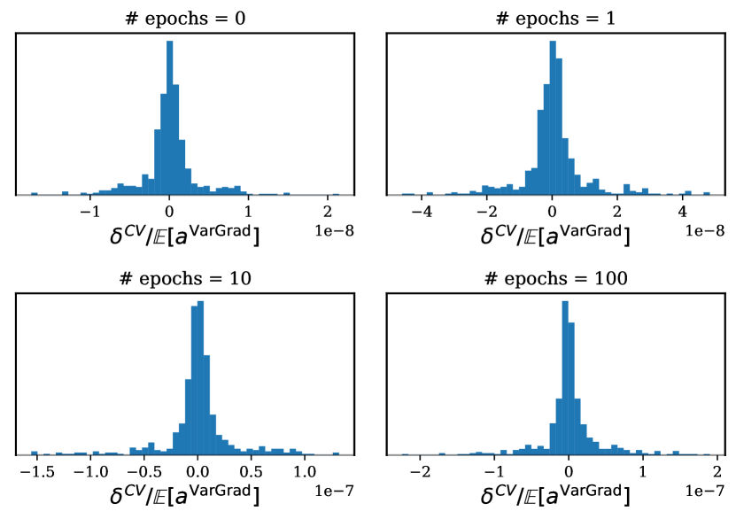
In Figure 2, we provide further evidence that this ratio is also small when fitting dvaes. Indeed, we observe that the ratio δiCV/𝔼[aVarGrad]superscriptsubscript𝛿𝑖CV𝔼delimited-[]superscript𝑎VarGrad\delta_{i}^{\textrm{CV}}/{\mathbb{E}}[a^{\textnormal{VarGrad}}] is typically very small and is distributed around zero during the whole optimisation procedure.
Refer to caption
(a) Two-layer linear dvae.
Refer to caption
(b) Non-linear dvae.
Figure 2: The distribution of δiCV𝔼[aVarGrad]superscriptsubscript𝛿𝑖CV𝔼delimited-[]superscript𝑎VarGrad\frac{\delta_{i}^{\text{CV}}}{\mathbb{E}[a^{\text{VarGrad}}]} associated with the biases of two dvae models with 200200200 latent dimensions trained on Omniglot using VarGrad. The estimates are obtained with 2,00020002{,}000 Monte Carlo samples. The ratio δiCV𝔼[aVarGrad]superscriptsubscript𝛿𝑖CV𝔼delimited-[]superscript𝑎VarGrad\frac{\delta_{i}^{\text{CV}}}{\mathbb{E}[a^{\text{VarGrad}}]} is consistently small throughout the optimisation procedure.

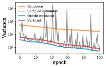
Variance reduction and computational cost.  In Figure 3 we show the variance of different gradient estimators throughout the optimisation in the logistic regression setting. We realise a significant improvement of VarGrad compared to the standard Reinforce estimator (Eq. 2). In fact, we observe a small difference between the variance of VarGrad and the variance of an oracle estimator based on Reinforce with access to the optimal control variate coefficient asuperscript𝑎a^{*}. Figure 3 also shows the variance of the sampled estimator, which is based on Reinforce with an estimate of the optimal control variate; this confirms the difficulty of estimating it in practice. (A similar trend can be observed for the dvae in the results in Appendix B, where VarGrad is compared to a wider list of estimators from the dvae literature.) All methods use S=4𝑆4S=4 Monte Carlo samples, and the control variate coefficient is estimated with either 222 extra samples (sampled estimator) or 1,00010001{,}000 samples (oracle estimator).

Refer to caption
Figure 3: Estimates of the variance of the gradient component w.r.t. the posterior mean of one of the weights for the logistic regression model. The variance of VarGrad is close to the oracle estimator based on Reinforce with access to the optimal control variate coefficient asuperscript𝑎a^{*}. Moreover, the sampled estimator (based on Reinforce with an estimate of asuperscript𝑎a^{*}) shows the difficulty of estimating the optimal control variate coefficient in practice.

Finally, Figure 4 compares VarGad with other estimators by training a dvae on Omniglot. The figure shows the negative elbo as a function of the epoch number (left plot) and against the wall-clock time (right plot). The negative elbo is computed on the standard test split and the optimisation uses Adam (Kingma and Ba, 2015) with learning rate of 0.0010.0010.001. VarGrad achieves similar performance to state-of-the-art estimators, such as rebar (Tucker et al., 2017), relax (Grathwohl et al., 2018), and arm (Yin and Zhou, 2019), while being simpler to implement (see Algorithm 1) and without any tunable hyperparameters.

Refer to caption
Figure 4: Optimisation trace versus epoch (left) and wall-clock time (right) for a two-layer linear dvae on a fixed binarisation of Omniglot. The plot compares VarGrad to Reinforce with score function control variates (Ranganath et al., 2014), dynamic rebar (Tucker et al., 2017), relax, relax + rebar (Grathwohl et al., 2018) and ARM (Yin and Zhou, 2019). The number of samples used to compute each gradient estimator is given in the figure legend. VarGrad demonstrates favourable scalability and performance when compared to the other estimators.

7 Conclusions

We have analysed the VarGrad estimator, an estimator of the gradient of the kl that is based on Reinforce with leave-one-out control variates, which was first introduced by Salimans and Knowles (2014) and Kool et al. (2019). We have established the connection between VarGrad and a novel divergence, which we call the log-variance loss. We have showed theoretically that, under certain conditions, the VarGrad control variate coefficients are close to the optimal ones. Moreover, we have established the conditions that guarantee that VarGrad exhibits lower variance than Reinforce. We leave it for future work to explore the direct optimisation of the log-variance loss for alternative choices of the reference distribution r(z)𝑟𝑧r(z).

Acknowledgments

Ö. D. A. and A. B. are funded by the Lloyds Register Foundation programme on Data Centric Engineering through the London Air Quality project at The Alan Turing Institute for Data Science and AI. This work was supported under EPSRC grant EP/N510129/1 as well as by Deutsche Forschungsgemeinschaft (DFG) through the grant CRC 1114 ‘Scaling Cascades in Complex Systems’ (projects A02 and A05, project number 235221301).

Broader Impact

Variational inference algorithms are approximate inference methods used in many practical applications, including computational neuroscience, natural language processing, and computer vision; see Blei et al. (2017). The performance of variational inference often depends on the variance of the gradient estimator of its objective. High-variance estimators can make the resulting algorithm unstable and unreliable to use in real-world deployment scenarios; hence, deeper theoretical and empirical understanding of different gradient estimators is crucial for safe applicability of these methods in real-world settings.

In our work, we provide an analysis of the VarGrad estimator. We show the connection between this estimator and the “log-variance loss” and demonstrate its relationship to the optimal score function control variate for Reinforce, providing a theoretical analysis. We support our theoretical analysis with empirical results. We believe our work contributes in the further understanding of variational inference methods and contributes to improving their safety and applicability.

While our theoretical results are suggestive, we warn that the bounds depend on the nature of the model at hand. Therefore, the use of the results here while ignoring the model-specific aspects of our assumptions may lead to some risks in application.

References

  • Blei et al. (2017) D. M. Blei, A. Kucukelbir, and J. D. McAuliffe. Variational inference: A review for statisticians. Journal of the American Statistical Association, 112(518):859–877, 2017.
  • Bradbury et al. (2018) J. Bradbury, R. Frostig, P. Hawkins, M. J. Johnson, C. Leary, D. Maclaurin, and S. Wanderman-Milne. JAX: composable transformations of Python+NumPy programs, 2018. URL http://github.com/google/jax.
  • Carbonetto et al. (2009) P. Carbonetto, M. King, and F. Hamze. A stochastic approximation method for inference in probabilistic graphical models. In Advances in Neural Information Processing Systems, 2009.
  • Cong et al. (2019) Y. Cong, M. Zhao, K. Bai, and L. Carin. GO gradient for expectation-based objectives. In International Conference on Learning Representations, 2019.
  • Cover and Thomas (2012) T. M. Cover and J. A. Thomas. Elements of Information Theory. John Wiley & Sons, 2012.
  • Dieng et al. (2017) A. B. Dieng, D. Tran, R. Ranganath, J. Paisley, and D. M. Blei. Variational inference via χ𝜒\chi-upper bound minimization. In Advances in Neural Information Processing Systems, 2017.
  • Dong et al. (2020) Z. Dong, A. Mnih, and G. Tucker. DisARM: An antithetic gradient estimator for binary latent variables. In Advances in Neural Information Processing Systems, 2020.
  • Ghosal et al. (2000) S. Ghosal, J. K. Ghosh, A. W. Van Der Vaart, et al. Convergence rates of posterior distributions. Annals of Statistics, 28(2):500–531, 2000.
  • Grathwohl et al. (2018) W. Grathwohl, D. Choi, Y. Wu, G. Roeder, and D. Duvenaud. Backpropagation through the void: Optimizing control variates for black-box gradient estimation. In International Conference on Learning Representations, 2018.
  • Gu et al. (2016) S. Gu, S. Levine, I. Sutskever, and A. Mnih. MuProp: Unbiased backpropagation for stochastic neural networks. In International Conference on Machine Learning, 2016.
  • Hennigan et al. (2020) T. Hennigan, T. Cai, T. Norman, and I. Babuschkin. Haiku: Sonnet for JAX, 2020. URL http://github.com/deepmind/dm-haiku.
  • Hernández-Lobato et al. (2016) Y. Hernández-Lobato, J. M. amd Li, M. Rowland, D. Hernández-Lobato, T. Bui, and R. E. Turner. Black-box α𝛼\alpha-divergence minimization. In International Conference on Machine Learning, 2016.
  • Jang et al. (2017) E. Jang, S. Gu, and B. Poole. Categorical reparameterization with Gumbel-softmax. In International Conference on Learning Representations, 2017.
  • Jordan et al. (1999) M. I. Jordan, Z. Ghahramani, T. S. Jaakkola, and L. K. Saul. An introduction to variational methods for graphical models. Machine Learning, 37(2):183–233, Nov. 1999.
  • Kingma and Ba (2015) D. P. Kingma and J. Ba. Adam: A method for stochastic optimization. In International Conference on Learning Representations (ICLR), 2015.
  • Kingma and Welling (2014) D. P. Kingma and M. Welling. Auto-encoding variational Bayes. In International Conference on Learning Representations, 2014.
  • Kool et al. (2019) W. Kool, H. van Hoof, and M. Welling. Buy 4 REINFORCE samples, get a baseline for free! In ICLR Workshop on Deep Reinforcement Learning Meets Structured Prediction, 2019.
  • Kool et al. (2020) W. Kool, H. van Hoof, and M. Welling. Estimating gradients for discrete random variables by sampling without replacement. In International Conference on Learning Representations, 2020.
  • Lake et al. (2015) B. M. Lake, R. Salakhutdinov, and J. B. Tenenbaum. Human-level concept learning through probabilistic program induction. Science, 350(6266):1332–1338, 2015.
  • Lee et al. (2018) W. Lee, H. Yu, and H. Yang. Reparameterization gradient for non-differentiable models. In Advances in Neural Information Processing Systems, 2018.
  • Li and Turner (2016) Y. Li and R. E. Turner. Rényi divergence variational inference. In Advances in Neural Information Processing Systems, 2016.
  • Maddison et al. (2017) C. J. Maddison, A. Mnih, and Y. W. Teh. The concrete distribution: A continuous relaxation of discrete random variables. In International Conference on Learning Representations, 2017.
  • Mnih and Gregor (2014) A. Mnih and K. Gregor. Neural variational inference and learning in belief networks. In International Conference on Machine Learning, 2014.
  • Mnih and Rezende (2016) A. Mnih and D. J. Rezende. Variational inference for Monte Carlo objectives. In International Conference on Machine Learning, 2016.
  • Mohamed et al. (2019) S. Mohamed, M. Rosca, M. Figurnov, and A. Mnih. Monte Carlo gradient estimation in machine learning. arXiv preprint arXiv:1906.10652, 2019.
  • Naesseth et al. (2017) C. Naesseth, F. J. R. Ruiz, S. Linderman, and D. M. Blei. Reparameterization gradients through acceptance-rejection methods. In Artificial Intelligence and Statistics, 2017.
  • Naesseth et al. (2020) C. A. Naesseth, F. Lindsten, and D. M. Blei. Markovian score climbing: Variational inference with kl(p||q)(p||q). arXiv preprint arXiv:2003.10374, 2020.
  • Nüsken and Richter (2020) N. Nüsken and L. Richter. Solving high-dimensional Hamilton-Jacobi-Bellman PDEs using neural networks: perspectives from the theory of controlled diffusions and measures on path space. arXiv preprint arXiv:2005.05409, 2020.
  • Paisley et al. (2012) J. W. Paisley, D. M. Blei, and M. I. Jordan. Variational Bayesian inference with stochastic search. In International Conference on Machine Learning, 2012.
  • Peters and Welling (2018) J. W. T. Peters and M. Welling. Probabilistic binary neural networks. arXiv preprint arXiv:1809.03368, 2018.
  • Ranganath et al. (2014) R. Ranganath, S. Gerrish, and D. M. Blei. Black box variational inference. In Artificial Intelligence and Statistics, 2014.
  • Ranganath et al. (2016) R. Ranganath, J. Altosaar, D. Tran, and D. M. Blei. Operator variational inference. In Advances in Neural Information Processing Systems, 2016.
  • Reiss (2012) R.-D. Reiss. Approximate distributions of order statistics: with applications to nonparametric statistics. Springer science & business media, 2012.
  • Rezende et al. (2014) D. J. Rezende, S. Mohamed, and D. Wierstra. Stochastic backpropagation and approximate inference in deep generative models. In International Conference on Machine Learning, 2014.
  • Robbins and Monro (1951) H. Robbins and S. Monro. A stochastic approximation method. Annals of Mathematical Statistics, 22:400–407, 1951.
  • Roeder et al. (2017) G. Roeder, Y. Wu, and D. Duvenaud. Sticking the landing: Simple, lower-variance gradient estimators for variational inference. In Advances in Neural Information Processing Systems, 2017.
  • Ruiz and Titsias (2019) F. J. R. Ruiz and M. K. Titsias. A contrastive divergence for combining variational inference and MCMC. In International Conference on Machine Learning, 2019.
  • Ruiz et al. (2016) F. J. R. Ruiz, M. K. Titsias, and D. M. Blei. The generalized reparameterization gradient. In Advances in Neural Information Processing Systems, 2016.
  • Salakhutdinov and Murray (2008) R. Salakhutdinov and I. Murray. On the quantitative analysis of deep belief networks. In Proceedings of the 25th international conference on Machine learning, pages 872–879, 2008.
  • Salimans and Knowles (2014) T. Salimans and D. A. Knowles. On using control variates with stochastic approximation for variational bayes and its connection to stochastic linear regression. arXiv preprint arXiv:1401.1022, 2014.
  • Shayer et al. (2018) O. Shayer, D. Levi, and E. Fetaya. Learning discrete weights using the local reparameterization trick. In International Conference on Learning Representations, 2018.
  • Titsias and Lázaro-Gredilla (2014) M. K. Titsias and M. Lázaro-Gredilla. Doubly stochastic variational Bayes for non-conjugate inference. In International Conference on Machine Learning, 2014.
  • Tucker et al. (2017) G. Tucker, A. Mnih, C. J. Maddison, and J. Sohl-Dickstein. REBAR: low-variance, unbiased gradient estimates for discrete latent variable models. In International Conference on Learning Representations, 2017.
  • Tucker et al. (2018) G. Tucker, D. Lawson, S. Gu, and C. J. Maddison. Doubly reparameterized gradient estimators for Monte Carlo objectives. In International Conference on Learning Representations, 2018.
  • Wang et al. (2018) D. Wang, H. Liu, and Q. Liu. Variational inference with tail-adaptive f𝑓f-divergence. In Advances in Neural Information Processing Systems, 2018.
  • Williams (1992) R. J. Williams. Simple statistical gradient-following algorithms for connectionist reinforcement learning. Machine Learning, 8(3–4):229–256, 1992.
  • Yin and Zhou (2019) M. Yin and M. Zhou. ARM: Augment-REINFORCE-merge gradient for stochastic binary networks. In International Conference on Learning Representations, 2019.
  • Yin et al. (2019) M. Yin, Y. Yue, and M. Zhou. ARSM: Augment-REINFORCE-swap-merge estimator for gradient backpropagation through categorical variables. In International Conference on Machine Learning, 2019.

Supplementary Material

Appendix A Proof of Paper Results

A.1 Proof of Proposition 1

Proof.

We first consider the gradient of the kl divergence. It is given by

ϕkl(qϕ(z)||p(z|x))=ϕqϕ(z)dz+log(qϕ(z)p(z|x))ϕqϕ(z)dz,\nabla_{\phi}\textrm{{kl}}(q_{\phi}(z)\;||\;p(z\,|\,x))=\int\nabla_{\phi}q_{\phi}(z)\,\mathrm{d}z+\int\log\left(\frac{q_{\phi}(z)}{p(z\,|\,x)}\right)\nabla_{\phi}q_{\phi}(z)\,\mathrm{d}z, (22)

where we can drop the first term since ϕqϕ(z)dz=ϕqϕ(z)dz=ϕ(1)=0subscriptitalic-ϕsubscript𝑞italic-ϕ𝑧differential-d𝑧subscriptitalic-ϕsubscript𝑞italic-ϕ𝑧differential-d𝑧subscriptitalic-ϕ10\int\nabla_{\phi}q_{\phi}(z)\,\mathrm{d}z=\nabla_{\phi}\int q_{\phi}(z)\,\mathrm{d}z=\nabla_{\phi}(1)=0.

We now consider the gradient of the log-variance loss. Using the definition from Eq. 5, we see that

ϕr(qϕ(z)||p(z|x))=12ϕlog2(qϕ(z)p(z|x))r(z)dz12ϕ(log(qϕ(z)p(z|x))r(z)dz)2\displaystyle\nabla_{\phi}\mathcal{L}_{r}(q_{\phi}(z)\;||\;p(z\,|\,x))=\frac{1}{2}\nabla_{\phi}\int\log^{2}\left(\frac{q_{\phi}(z)}{p(z\,|\,x)}\right)r(z)\,{\mathrm{d}}z-\frac{1}{2}\nabla_{\phi}\left(\int\log\left(\frac{q_{\phi}(z)}{p(z\,|\,x)}\right)r(z)\,{\mathrm{d}}z\right)^{2}
=log(qϕ(z)p(z|x))ϕqϕ(z)qϕ(z)r(z)dz(log(qϕ(z)p(z|x))r(z)dz)(ϕqϕ(z)qϕ(z)r(z)dz).absentsubscript𝑞italic-ϕ𝑧𝑝conditional𝑧𝑥subscriptitalic-ϕsubscript𝑞italic-ϕ𝑧subscript𝑞italic-ϕ𝑧𝑟𝑧differential-d𝑧subscript𝑞italic-ϕ𝑧𝑝conditional𝑧𝑥𝑟𝑧differential-d𝑧subscriptitalic-ϕsubscript𝑞italic-ϕ𝑧subscript𝑞italic-ϕ𝑧𝑟𝑧differential-d𝑧\displaystyle=\int\log\left(\frac{q_{\phi}(z)}{p(z\,|\,x)}\right)\frac{\nabla_{\phi}q_{\phi}(z)}{q_{\phi}(z)}r(z)\,{\mathrm{d}}z-\left(\int\log\left(\frac{q_{\phi}(z)}{p(z\,|\,x)}\right)r(z)\,{\mathrm{d}}z\right)\left(\int\frac{\nabla_{\phi}q_{\phi}(z)}{q_{\phi}(z)}r(z)\,{\mathrm{d}}z\right).

When we evaluate the gradient at r(z)=qϕ(z)𝑟𝑧subscript𝑞italic-ϕ𝑧r(z)=q_{\phi}(z), the right-most term vanishes, since ϕqϕ(z)r(z)r(z)dz=ϕqϕ(z)dz=0subscriptitalic-ϕsubscript𝑞italic-ϕ𝑧𝑟𝑧𝑟𝑧differential-d𝑧subscriptitalic-ϕsubscript𝑞italic-ϕ𝑧differential-d𝑧0\int\frac{\nabla_{\phi}q_{\phi}(z)}{r(z)}r(z)\,{\mathrm{d}}z=\int\nabla_{\phi}q_{\phi}(z)\,{\mathrm{d}}z=0. Thus, the gradient of the log-variance loss becomes equal to the gradient of the kl divergence. \Box

A.2 Proof of Lemma 1

Proof.

First, notice that Varqϕ(ϕilogqϕ)=𝔼qϕ[(ϕilogqϕ)2]subscriptVarsubscript𝑞italic-ϕsubscriptsubscriptitalic-ϕ𝑖subscript𝑞italic-ϕsubscript𝔼subscript𝑞italic-ϕdelimited-[]superscriptsubscriptsubscriptitalic-ϕ𝑖subscript𝑞italic-ϕ2\operatorname{Var}_{q_{\phi}}\left(\partial_{\phi_{i}}\log q_{\phi}\right)=\mathbb{E}_{q_{\phi}}[(\partial_{\phi_{i}}\log q_{\phi})^{2}] since 𝔼qϕ[ϕilogqϕ]=0subscript𝔼subscript𝑞italic-ϕdelimited-[]subscriptsubscriptitalic-ϕ𝑖subscript𝑞italic-ϕ0\mathbb{E}_{q_{\phi}}[\partial_{\phi_{i}}\log q_{\phi}]=0. We then compute

aisuperscriptsubscript𝑎𝑖\displaystyle a_{i}^{*} =𝔼qϕ[fϕ(ϕilogqϕ)2]𝔼qϕ[(ϕilogqϕ)2]absentsubscript𝔼subscript𝑞italic-ϕdelimited-[]subscript𝑓italic-ϕsuperscriptsubscriptsubscriptitalic-ϕ𝑖subscript𝑞italic-ϕ2subscript𝔼subscript𝑞italic-ϕdelimited-[]superscriptsubscriptsubscriptitalic-ϕ𝑖subscript𝑞italic-ϕ2\displaystyle=\frac{\mathbb{E}_{q_{\phi}}\left[f_{\phi}(\partial_{\phi_{i}}\log q_{\phi})^{2}\right]}{\mathbb{E}_{q_{\phi}}\left[\left(\partial_{\phi_{i}}\log q_{\phi}\right)^{2}\right]} (23)
=𝔼qϕ[fϕ(ϕilogqϕ)2]𝔼qϕ[fϕ]𝔼qϕ[(ϕilogqϕ)2]+𝔼qϕ[fϕ]𝔼qϕ[(ϕilogqϕ)2]𝔼qϕ[(ϕilogqϕ)2]absentsubscript𝔼subscript𝑞italic-ϕdelimited-[]subscript𝑓italic-ϕsuperscriptsubscriptsubscriptitalic-ϕ𝑖subscript𝑞italic-ϕ2subscript𝔼subscript𝑞italic-ϕdelimited-[]subscript𝑓italic-ϕsubscript𝔼subscript𝑞italic-ϕdelimited-[]superscriptsubscriptsubscriptitalic-ϕ𝑖subscript𝑞italic-ϕ2subscript𝔼subscript𝑞italic-ϕdelimited-[]subscript𝑓italic-ϕsubscript𝔼subscript𝑞italic-ϕdelimited-[]superscriptsubscriptsubscriptitalic-ϕ𝑖subscript𝑞italic-ϕ2subscript𝔼subscript𝑞italic-ϕdelimited-[]superscriptsubscriptsubscriptitalic-ϕ𝑖subscript𝑞italic-ϕ2\displaystyle=\frac{\mathbb{E}_{q_{\phi}}\left[f_{\phi}(\partial_{\phi_{i}}\log q_{\phi})^{2}\right]-\mathbb{E}_{q_{\phi}}\left[f_{\phi}\right]\mathbb{E}_{q_{\phi}}\left[(\partial_{\phi_{i}}\log q_{\phi})^{2}\right]+\mathbb{E}_{q_{\phi}}\left[f_{\phi}\right]\mathbb{E}_{q_{\phi}}\left[(\partial_{\phi_{i}}\log q_{\phi})^{2}\right]}{\mathbb{E}_{q_{\phi}}\left[\left(\partial_{\phi_{i}}\log q_{\phi}\right)^{2}\right]} (24)
=𝔼qϕ[f¯ϕ]+δiCV.absentsubscript𝔼subscript𝑞italic-ϕdelimited-[]subscript¯𝑓italic-ϕsubscriptsuperscript𝛿CV𝑖\displaystyle=\mathbb{E}_{q_{\phi}}[\bar{f}_{\phi}]+\delta^{\text{CV}}_{i}. (25)

In the last line we have used the fact that 𝔼qϕ[fϕ]=𝔼qϕ[f¯ϕ]subscript𝔼subscript𝑞italic-ϕdelimited-[]subscript𝑓italic-ϕsubscript𝔼subscript𝑞italic-ϕdelimited-[]subscript¯𝑓italic-ϕ\mathbb{E}_{q_{\phi}}[f_{\phi}]=\mathbb{E}_{q_{\phi}}[\bar{f}_{\phi}]. \Box

A.3 Proof of Proposition 16

Proof.

Note that

|δiCV𝔼qϕ[aVarGrad]|=|Covqϕ(fϕ,(ϕilogqϕ)2)𝔼qϕ[fϕ]Varqϕ(ϕilogqϕ)|=|𝔼qϕ[(fϕ𝔼qϕ[fϕ])(ϕilogqϕ)2]𝔼qϕ[fϕ]𝔼qϕ[(ϕilogqϕ)2]|,subscriptsuperscript𝛿CV𝑖subscript𝔼subscript𝑞italic-ϕdelimited-[]superscript𝑎VarGradsubscriptCovsubscript𝑞italic-ϕsubscript𝑓italic-ϕsuperscriptsubscriptsubscriptitalic-ϕ𝑖subscript𝑞italic-ϕ2subscript𝔼subscript𝑞italic-ϕdelimited-[]subscript𝑓italic-ϕsubscriptVarsubscript𝑞italic-ϕsubscriptsubscriptitalic-ϕ𝑖subscript𝑞italic-ϕsubscript𝔼subscript𝑞italic-ϕdelimited-[]subscript𝑓italic-ϕsubscript𝔼subscript𝑞italic-ϕdelimited-[]subscript𝑓italic-ϕsuperscriptsubscriptsubscriptitalic-ϕ𝑖subscript𝑞italic-ϕ2subscript𝔼subscript𝑞italic-ϕdelimited-[]subscript𝑓italic-ϕsubscript𝔼subscript𝑞italic-ϕdelimited-[]superscriptsubscriptsubscriptitalic-ϕ𝑖subscript𝑞italic-ϕ2\displaystyle\left|\frac{\delta^{\text{CV}}_{i}}{\mathbb{E}_{q_{\phi}}[a^{\text{VarGrad}}]}\right|=\left|\frac{\operatorname{Cov}_{q_{\phi}}\left(f_{\phi},\left(\partial_{\phi_{i}}\log q_{\phi}\right)^{2}\right)}{\mathbb{E}_{q_{\phi}}[f_{\phi}]\operatorname{Var}_{q_{\phi}}\left(\partial_{\phi_{i}}\log q_{\phi}\right)}\right|=\left|\frac{\mathbb{E}_{q_{\phi}}\left[(f_{\phi}-\mathbb{E}_{q_{\phi}}[f_{\phi}])\left(\partial_{\phi_{i}}\log q_{\phi}\right)^{2}\right]}{\mathbb{E}_{q_{\phi}}[f_{\phi}]\mathbb{E}_{q_{\phi}}\left[(\partial_{\phi_{i}}\log q_{\phi})^{2}\right]}\right|, (26)

where we have used the fact that 𝔼qϕ[ϕilogqϕ]=0subscript𝔼subscript𝑞italic-ϕdelimited-[]subscriptsubscriptitalic-ϕ𝑖subscript𝑞italic-ϕ0\mathbb{E}_{q_{\phi}}[\partial_{\phi_{i}}\log q_{\phi}]=0. From

𝔼[fϕ]=ELBO(ϕ)=KL(qϕ(z)||p(z|x))logp(x),\mathbb{E}[f_{\phi}]=-\mathrm{ELBO}(\phi)=\mathrm{KL}(q_{\phi}(z)\;||\;p(z|x))-\log p(x),

and using the Cauchy-Schwarz inequality, Eq. 26 can be bounded from above by

(Varqϕ(logqϕ(z)p(z|x)))1/2|KL(qϕ(z)||p(z|x))logp(x)|(𝔼qϕ[(ϕilogqϕ)4](𝔼qϕ[(ϕilogqϕ)2])2)1/2.\frac{\left(\operatorname{Var}_{q_{\phi}}\left(\log\frac{q_{\phi}(z)}{p(z|x)}\right)\right)^{1/2}}{|\mathrm{KL}(q_{\phi}(z)\;||\;p(z|x))-\log p(x)|}\left(\frac{\mathbb{E}_{q_{\phi}}[(\partial_{\phi_{i}}\log q_{\phi})^{4}]}{(\mathbb{E}_{q_{\phi}}[(\partial_{\phi_{i}}\log q_{\phi})^{2}])^{2}}\right)^{1/2}. (27)

The second factor equals Kurt[ϕilogqϕ]\sqrt{\mathrm{Kurt}[\partial_{\phi_{i}}\log q_{\phi}}]. To bound the first factor, notice that

(Varqϕ(logqϕ(z)p(z|x)))1/2(𝔼qϕ[log2qϕ(z)p(z|x)])1/2=(𝔼qϕ[log2p(z|x)qϕ(z)])1/2superscriptsubscriptVarsubscript𝑞italic-ϕsubscript𝑞italic-ϕ𝑧𝑝conditional𝑧𝑥12superscriptsubscript𝔼subscript𝑞italic-ϕdelimited-[]superscript2subscript𝑞italic-ϕ𝑧𝑝conditional𝑧𝑥12superscriptsubscript𝔼subscript𝑞italic-ϕdelimited-[]superscript2𝑝conditional𝑧𝑥subscript𝑞italic-ϕ𝑧12\displaystyle\left(\operatorname{Var}_{q_{\phi}}\left(\log\frac{q_{\phi}(z)}{p(z|x)}\right)\right)^{1/2}\leq\left(\mathbb{E}_{q_{\phi}}\left[\log^{2}\frac{q_{\phi}(z)}{p(z|x)}\right]\right)^{1/2}=\left(\mathbb{E}_{q_{\phi}}\left[\log^{2}\frac{p(z|x)}{q_{\phi}(z)}\right]\right)^{1/2} (28)
(2𝔼qϕ[exp(|logp(z|x)qϕ(z)|)1|logp(z|x)qϕ(z)|])1/2,absentsuperscript2subscript𝔼subscript𝑞italic-ϕdelimited-[]𝑝conditional𝑧𝑥subscript𝑞italic-ϕ𝑧1𝑝conditional𝑧𝑥subscript𝑞italic-ϕ𝑧12\displaystyle\leq\left(2\mathbb{E}_{q_{\phi}}\left[\exp\left(\left|\log\frac{p(z|x)}{q_{\phi}(z)}\right|\right)-1-\left|\log\frac{p(z|x)}{q_{\phi}(z)}\right|\right]\right)^{1/2}, (29)

where we have used the estimate

ex1x=n=0xnn!1x=n=2xnn!12x2,x0,formulae-sequencesuperscript𝑒𝑥1𝑥superscriptsubscript𝑛0superscript𝑥𝑛𝑛1𝑥superscriptsubscript𝑛2superscript𝑥𝑛𝑛12superscript𝑥2𝑥0e^{x}-1-x=\sum_{n=0}^{\infty}\frac{x^{n}}{n!}-1-x=\sum_{n=2}^{\infty}\frac{x^{n}}{n!}\geq\frac{1}{2}x^{2},\quad x\geq 0, (30)

with x=|logp(z|x)qϕ(z)|𝑥𝑝conditional𝑧𝑥subscript𝑞italic-ϕ𝑧x=\left|\log\frac{p(z|x)}{q_{\phi}(z)}\right|. We now use [Ghosal et al., 2000, Lemma 8.3] to bound Eq. 29 from above by

2Ch(qϕ(z)||p(z|x)),2\sqrt{C}h(q_{\phi}(z)\;||\;p(z|x)), (31)

where

h(qϕ(z)||p(z|x))=(qϕ(z)p(z|x))2dzh(q_{\phi}(z)\;||\;p(z|x))=\sqrt{\int\left(\sqrt{q_{\phi}(z)}-\sqrt{p(z|x)}\right)^{2}\,\mathrm{d}z} (32)

is the Hellinger distance. From [Reiss, 2012, Lemma A.3.5] we have the bound h(qϕ(z)||p(z|x))KL(qϕ(z)||p(z|x))h(q_{\phi}(z)\;||\;p(z|x))\leq\sqrt{\mathrm{KL}(q_{\phi}(z)\;||\;p(z|x))}. Combining these estimates we arrive at the claimed result. \Box

A.4 Proof of Proposition 3

Proof.

We start by defining the short-cuts

A=fϕ(z),B=(ϕilogqϕ)(z).formulae-sequence𝐴subscript𝑓italic-ϕ𝑧𝐵subscriptsubscriptitalic-ϕ𝑖subscript𝑞italic-ϕ𝑧A=f_{\phi}(z),\qquad B=\left(\partial_{\phi_{i}}\log q_{\phi}\right)(z). (33)

Let us compute the difference of the variances of the estimators to leading order in S𝑆S, namely

Var(g^Reinforce,i)Var(g^VarGrad,i)=1SVar(AB)+S2S(S1)𝔼[(A𝔼[A])(B𝔼[B])]2\displaystyle\operatorname{Var}(\widehat{g}_{\text{Reinforce},i})-\operatorname{Var}(\widehat{g}_{\text{VarGrad},i})=\frac{1}{S}\operatorname{Var}(AB)+\frac{S-2}{S(S-1)}\operatorname{\mathbb{E}}\left[(A-\operatorname{\mathbb{E}}[A])(B-\operatorname{\mathbb{E}}[B])\right]^{2} (34a)
Var(A)Var(B)S(S1)1S𝔼[(A𝔼[A])2(B𝔼[B])2]Var𝐴Var𝐵𝑆𝑆11𝑆𝔼superscript𝐴𝔼𝐴2superscript𝐵𝔼𝐵2\displaystyle\qquad-\frac{\operatorname{Var}(A)\operatorname{Var}(B)}{S(S-1)}-\frac{1}{S}\operatorname{\mathbb{E}}\left[(A-\operatorname{\mathbb{E}}[A])^{2}(B-\operatorname{\mathbb{E}}[B])^{2}\right] (34b)
=1S(𝔼[A2B2]𝔼[AB]2)+S2S(S1)𝔼[AB]2\displaystyle=\frac{1}{S}\left(\operatorname{\mathbb{E}}\left[A^{2}B^{2}\right]-\operatorname{\mathbb{E}}[AB]^{2}\right)+\frac{S-2}{S(S-1)}\operatorname{\mathbb{E}}[AB]^{2} (34c)
1S(𝔼[A2B2]2𝔼[A]𝔼[AB2]+𝔼[A]2𝔼[B2])+𝒪(1S2)\displaystyle\qquad-\frac{1}{S}\left(\operatorname{\mathbb{E}}\left[A^{2}B^{2}\right]-2\operatorname{\mathbb{E}}[A]\operatorname{\mathbb{E}}\left[AB^{2}\right]+\operatorname{\mathbb{E}}[A]^{2}\operatorname{\mathbb{E}}\left[B^{2}\right]\right)+\mathcal{O}\left(\frac{1}{S^{2}}\right) (34d)
=1S(S1)𝔼[AB]21S𝔼[A](𝔼[A]𝔼[B2]2𝔼[AB2])+𝒪(1S2)\displaystyle=-\frac{1}{S(S-1)}\operatorname{\mathbb{E}}[AB]^{2}-\frac{1}{S}\operatorname{\mathbb{E}}[A]\left(\operatorname{\mathbb{E}}[A]\operatorname{\mathbb{E}}\left[B^{2}\right]-2\operatorname{\mathbb{E}}\left[AB^{2}\right]\right)+\mathcal{O}\left(\frac{1}{S^{2}}\right) (34e)
=1S𝔼[A](2𝔼[AB2]𝔼[A]𝔼[B2])+𝒪(1S2)absent1𝑆𝔼𝐴2𝔼𝐴superscript𝐵2𝔼𝐴𝔼superscript𝐵2𝒪1superscript𝑆2\displaystyle=\frac{1}{S}\operatorname{\mathbb{E}}[A]\left(2\operatorname{\mathbb{E}}\left[AB^{2}\right]-\operatorname{\mathbb{E}}[A]\operatorname{\mathbb{E}}\left[B^{2}\right]\right)+\mathcal{O}\left(\frac{1}{S^{2}}\right) (34f)
=1S𝔼[A]𝔼[B2](2δiCV+𝔼[A])+𝒪(1S2)absent1𝑆𝔼𝐴𝔼superscript𝐵22superscriptsubscript𝛿𝑖CV𝔼𝐴𝒪1superscript𝑆2\displaystyle=\frac{1}{S}\operatorname{\mathbb{E}}[A]\operatorname{\mathbb{E}}\left[B^{2}\right]\left(2\delta_{i}^{\text{CV}}+\operatorname{\mathbb{E}}[A]\right)+\mathcal{O}\left(\frac{1}{S^{2}}\right) (34g)
and we note that with 𝔼[B2]>0𝔼superscript𝐵20\operatorname{\mathbb{E}}\left[B^{2}\right]>0 the leading term is positive if
𝔼[A]δiCV+12𝔼[A]2>0,\displaystyle\operatorname{\mathbb{E}}[A]\delta_{i}^{\text{CV}}+\frac{1}{2}\operatorname{\mathbb{E}}[A]^{2}>0, (34h)

which is equivalent to the statement in the proposition. \Box

A.5 Proof of Corollary 1

Proof.

Note that with Proposition 16 we have

|δiCV𝔼qϕ[aVarGrad]|0subscriptsuperscript𝛿CV𝑖subscript𝔼subscript𝑞italic-ϕdelimited-[]superscript𝑎VarGrad0\displaystyle\left|\frac{\delta^{\text{CV}}_{i}}{\mathbb{E}_{q_{\phi}}[a^{\text{VarGrad}}]}\right|\to 0 (35)

for D𝐷D\to\infty, assuming that kl(qϕ(z)||p(z|x))\textrm{{kl}}(q_{\phi}(z)\;||\;p(z\,|\,x)) is strictly increasing in D𝐷D. Therefore, for large enough D𝐷D, the condition from Proposition 3 (see Eq. 19), is fulfilled and the statement follows immediately. \Box

A.6 Results on the Kurtosis of the Score for Exponential Families

Here we provide a more explicit expression for Kurt[ϕilogqϕ]Kurtdelimited-[]subscriptsubscriptitalic-ϕ𝑖subscript𝑞italic-ϕ\mathrm{Kurt}[\partial_{\phi_{i}}\log q_{\phi}] in the case when qϕ(z)subscript𝑞italic-ϕ𝑧q_{\phi}(z) is given by an exponential family, i.e. qϕ(z)=h(z)exp(ϕT(z)A(ϕ))subscript𝑞italic-ϕ𝑧𝑧superscriptitalic-ϕtop𝑇𝑧𝐴italic-ϕq_{\phi}(z)=h(z)\exp\left(\phi^{\top}T(z)-A(\phi)\right), where T(z)𝑇𝑧T(z) is the vector of sufficient statistics and A(ϕ)𝐴italic-ϕA(\phi) denotes the log-partition function. As an application, we show that in the Gaussian case, Kurt[ϕilogqϕ]Kurtdelimited-[]subscriptsubscriptitalic-ϕ𝑖subscript𝑞italic-ϕ\mathrm{Kurt}[\partial_{\phi_{i}}\log q_{\phi}] is uniformly bounded across the whole variational family.

Lemma 2.

Let qϕ(z)=h(z)exp(ϕT(z)A(ϕ))subscript𝑞italic-ϕ𝑧𝑧superscriptitalic-ϕtop𝑇𝑧𝐴italic-ϕq_{\phi}(z)=h(z)\exp\left(\phi^{\top}T(z)-A(\phi)\right). Then

Kurt[ϕilogqϕ]=𝔼qϕ[(Ti(z)mi)4]𝔼qϕ[(Ti(z)mi)2]2,Kurtdelimited-[]subscriptsubscriptitalic-ϕ𝑖subscript𝑞italic-ϕsubscript𝔼subscript𝑞italic-ϕdelimited-[]superscriptsubscript𝑇𝑖𝑧subscript𝑚𝑖4subscript𝔼subscript𝑞italic-ϕsuperscriptdelimited-[]superscriptsubscript𝑇𝑖𝑧subscript𝑚𝑖22\mathrm{Kurt}[\partial_{\phi_{i}}\log q_{\phi}]=\frac{{\mathbb{E}}_{q_{\phi}}\left[(T_{i}(z)-m_{i})^{4}\right]}{{\mathbb{E}}_{q_{\phi}}\left[(T_{i}(z)-m_{i})^{2}\right]^{2}}, (36)

where mi=𝔼qϕ[Ti(z)]subscript𝑚𝑖subscript𝔼subscript𝑞italic-ϕdelimited-[]subscript𝑇𝑖𝑧m_{i}={\mathbb{E}}_{q_{\phi}}[T_{i}(z)] denotes the mean of the sufficient statistics. In particular, Kurt[ϕilogqϕ]Kurtdelimited-[]subscriptsubscriptitalic-ϕ𝑖subscript𝑞italic-ϕ\mathrm{Kurt}[\partial_{\phi_{i}}\log q_{\phi}] does not depend on h(z)𝑧h(z) or A(ϕ)𝐴italic-ϕA(\phi).

Proof.

The claim follows by direct calculation. Indeed,

ϕilogqϕ(z)=Ti(z)Aϕi(ϕ).subscriptsubscriptitalic-ϕ𝑖subscript𝑞italic-ϕ𝑧subscript𝑇𝑖𝑧𝐴subscriptitalic-ϕ𝑖italic-ϕ\displaystyle\partial_{\phi_{i}}\log q_{\phi}(z)=T_{i}(z)-\frac{\partial A}{\partial\phi_{i}}(\phi). (37)

It is left to show that Aϕi(ϕ)=μi𝐴subscriptitalic-ϕ𝑖italic-ϕsubscript𝜇𝑖\frac{\partial A}{\partial\phi_{i}}(\phi)=\mu_{i}. For this, notice that the normalisation condition

h(z)exp(ϕT(z)A(ϕ))dz=1𝑧superscriptitalic-ϕtop𝑇𝑧𝐴italic-ϕdifferential-d𝑧1\int h(z)\exp\left(\phi^{\top}T(z)-A(\phi)\right)\mathrm{d}z=1 (38)

implies

h(z)(Ti(z)A(ϕ)ϕi)exp(ϕT(z)A(ϕ))dz=0𝑧subscript𝑇𝑖𝑧𝐴italic-ϕsubscriptitalic-ϕ𝑖superscriptitalic-ϕtop𝑇𝑧𝐴italic-ϕdifferential-d𝑧0\int h(z)\left(T_{i}(z)-\frac{\partial A(\phi)}{\partial\phi_{i}}\right)\exp\left(\phi^{\top}T(z)-A(\phi)\right)\mathrm{d}z=0 (39)

by taking the derivative w.r.t. ϕisubscriptitalic-ϕ𝑖\phi_{i}. The left-hand side equals 𝔼qϕ[Ti(z)]Aϕi(ϕ)subscript𝔼subscript𝑞italic-ϕdelimited-[]subscript𝑇𝑖𝑧𝐴subscriptitalic-ϕ𝑖italic-ϕ\mathbb{E}_{q_{\phi}}[T_{i}(z)]-\frac{\partial A}{\partial\phi_{i}}(\phi), and so the claim follows. \Box

Lemma 3.

Let qϕ(z)subscript𝑞italic-ϕ𝑧q_{\phi}(z) be the family of one-dimensional Gaussian distributions. Then there exists a constant K>0𝐾0K>0 such that

Kurt[ϕilogqϕ]<KKurtdelimited-[]subscriptsubscriptitalic-ϕ𝑖subscript𝑞italic-ϕ𝐾\mathrm{Kurt}[\partial_{\phi_{i}}\log q_{\phi}]<K (40)

for all i𝑖i and all ϕΦitalic-ϕΦ\phi\in\Phi. In fact, it is possible to take K=15𝐾15K=15.

Proof.

For the Gaussian family, the sufficient statistics are given by T1(z)=zsubscript𝑇1𝑧𝑧T_{1}(z)=z and T2(z)=z2subscript𝑇2𝑧superscript𝑧2T_{2}(z)=z^{2}. We have that

𝔼𝒩(μ,σ2)[(T1(z)m1)4]𝔼𝒩(μ,σ2)[(T1(z)m1)2]2=𝔼𝒩(μ,σ2)[(zμ)4]𝔼𝒩(μ,σ2)[(zμ)2]2=3,subscript𝔼𝒩𝜇superscript𝜎2delimited-[]superscriptsubscript𝑇1𝑧subscript𝑚14subscript𝔼𝒩𝜇superscript𝜎2superscriptdelimited-[]superscriptsubscript𝑇1𝑧subscript𝑚122subscript𝔼𝒩𝜇superscript𝜎2delimited-[]superscript𝑧𝜇4subscript𝔼𝒩𝜇superscript𝜎2superscriptdelimited-[]superscript𝑧𝜇223\frac{{\mathbb{E}}_{\mathcal{N}(\mu,\sigma^{2})}\left[(T_{1}(z)-m_{1})^{4}\right]}{{\mathbb{E}}_{\mathcal{N}(\mu,\sigma^{2})}\left[(T_{1}(z)-m_{1})^{2}\right]^{2}}=\frac{{\mathbb{E}}_{\mathcal{N}(\mu,\sigma^{2})}\left[(z-\mu)^{4}\right]}{{\mathbb{E}}_{\mathcal{N}(\mu,\sigma^{2})}\left[(z-\mu)^{2}\right]^{2}}=3, (41)

by the well-known fact the standard kurtosis of any univariate Gaussian is 333. A lengthy but straightforward computation shows that

𝔼𝒩(μ,σ2)[(T2(z)m2)4]𝔼𝒩(μ,σ2)[(T2(z)m2)2]2=3(4μ4+20μ2σ2+5σ4)(2μ2+σ2)2,subscript𝔼𝒩𝜇superscript𝜎2delimited-[]superscriptsubscript𝑇2𝑧subscript𝑚24subscript𝔼𝒩𝜇superscript𝜎2superscriptdelimited-[]superscriptsubscript𝑇2𝑧subscript𝑚22234superscript𝜇420superscript𝜇2superscript𝜎25superscript𝜎4superscript2superscript𝜇2superscript𝜎22\frac{{\mathbb{E}}_{\mathcal{N}(\mu,\sigma^{2})}\left[(T_{2}(z)-m_{2})^{4}\right]}{{\mathbb{E}}_{\mathcal{N}(\mu,\sigma^{2})}\left[(T_{2}(z)-m_{2})^{2}\right]^{2}}=\frac{3(4\mu^{4}+20\mu^{2}\sigma^{2}+5\sigma^{4})}{(2\mu^{2}+\sigma^{2})^{2}}, (42)

which is maximised for μ=0𝜇0\mu=0, taking the value 151515. \Box

Lemma 3 shows that the kurtosis term in our bound Eq. 16 can be bounded for Gaussian families. This result is expected to extend to the multivariate cases as well. We note that we observe in our experiments that the bound is finite in a variety of cases.

A.7 Dimension-dependence of the KLKL\mathrm{KL}-divergence

The following lemma shows that the KLKL\mathrm{KL}-divergence increases with the number of dimensions. This result follows from the chain-rule of KL divergence, see, e.g., Cover and Thomas [2012].

Lemma 4.

Let u(D)(z1,,zD)superscript𝑢𝐷subscript𝑧1subscript𝑧𝐷u^{(D)}(z_{1},\ldots,z_{D}) and v(D)(z1,,zD)superscript𝑣𝐷subscript𝑧1subscript𝑧𝐷v^{(D)}(z_{1},\ldots,z_{D}) be two arbitrary probability distributions on Dsuperscript𝐷\mathbb{R}^{D}. For J{1,D}𝐽1𝐷J\in\{1\ldots,D\} denote their marginals on the first J𝐽J coordinates by u(J)superscript𝑢𝐽u^{(J)} and v(J)superscript𝑣𝐽v^{(J)}, i.e.

u(J)(z1,,zJ)=∫⋯∫u(D)(z1,,zD)dzJ+1dzD,superscript𝑢𝐽subscript𝑧1subscript𝑧𝐽multiple-integralsuperscript𝑢𝐷subscript𝑧1subscript𝑧𝐷differential-dsubscript𝑧𝐽1differential-dsubscript𝑧𝐷u^{(J)}(z_{1},\ldots,z_{J})=\idotsint u^{(D)}(z_{1},\ldots,z_{D})\,\mathrm{d}z_{J+1}\ldots\mathrm{d}z_{D}, (43)

and

v(J)(z1,,zJ)=∫⋯∫v(D)(z1,,zD)dzJ+1dzD.superscript𝑣𝐽subscript𝑧1subscript𝑧𝐽multiple-integralsuperscript𝑣𝐷subscript𝑧1subscript𝑧𝐷differential-dsubscript𝑧𝐽1differential-dsubscript𝑧𝐷v^{(J)}(z_{1},\ldots,z_{J})=\idotsint v^{(D)}(z_{1},\ldots,z_{D})\,\mathrm{d}z_{J+1}\ldots\mathrm{d}z_{D}. (44)

Then

KL(u(1)||v(1))KL(u(2)||v(2))KL(u(D)||v(D)),\mathrm{KL}(u^{(1)}\;||\;v^{(1)})\leq\mathrm{KL}(u^{(2)}\;||\;v^{(2)})\leq\ldots\leq\mathrm{KL}(u^{(D)}\;||\;v^{(D)}), (45)

i.e. the function JKL(u(J)||v(J))J\mapsto\mathrm{KL}(u^{(J)}\;||\;v^{(J)}) is increasing.

Appendix B Details of Experimental Setup and Additional Results

B.1 Details of the Experiments

B.1.1 Logistic Regression

This section describes the experimental setup of the Bayesian logistic regression example which was discussed in the main text in Section 6.

Data.  We use a synthetic dataset with N=100𝑁100N=100, where input-output pairs are generated as follows: we sample a design matrix XN×D𝑋superscript𝑁𝐷X\in\mathbb{R}^{N\times D} for the inputs uniformly on [1,1]11[-1,1], random weights 𝐰D𝐰superscript𝐷{\mathbf{w}}\in\mathbb{R}^{D} from 𝒩(0,25IdD×D)𝒩025subscriptId𝐷𝐷\mathcal{N}(0,25\,\text{Id}_{D\times D}) and a random bias b𝑏b\in\mathbb{R} from 𝒩(0,1)𝒩01\mathcal{N}(0,1). We set 𝐩=σ(X𝐰+b 1)𝐩𝜎𝑋𝐰𝑏1\mathbf{p}=\sigma(X{\mathbf{w}}+b\,\mathbf{1}), where 𝟏1\mathbf{1} is an N𝑁N-dimensional vector of ones and σ(x)=11+exp(x)𝜎𝑥11𝑥\sigma(x)=\frac{1}{1+\exp(-x)} is the logistic sigmoid applied elementwise. Finally, we sample the outputs YBernoulli(𝐩)similar-to𝑌Bernoulli𝐩Y\sim\text{Bernoulli}(\mathbf{p}).

Approximate Posterior.  For this model, we set the approximate posterior to a diagonal Gaussian with free mean and log standard deviation parameters.

Training.  For all the experiments listed in the main text, we use the VarGrad estimator for the gradients of the logistic regression models. We train the models using stochastic gradient descent [Robbins and Monro, 1951] with a learning rate of 0.0010.0010.001.

Estimation of intractable quantities.  To estimate the intractable quantities in Figure 1, we use Monte Carlo sampling with 2000 samples for δCVsuperscript𝛿CV\delta^{\text{CV}} and 𝔼qϕ[aVarGrad]subscript𝔼subscript𝑞italic-ϕdelimited-[]superscript𝑎VarGrad\mathbb{E}_{q_{\phi}}[a^{\text{VarGrad}}]. We estimate the KL divergence with the identity KL(qϕ(z)p(z|x))=logp(x)ELBO(ϕ)\textsc{KL}(q_{\phi}(z)\|p(z|x))=\log p(x)-\text{ELBO}(\phi), where logp(x)𝑝𝑥\log p(x) is estimated using importance sampling with 100001000010000 samples and ELBO(ϕ)ELBOitalic-ϕ\text{ELBO}(\phi) using standard Monte Carlo sampling with 2000 samples.

For the variance estimates in Figure 3, we use 1000 Monte Carlo samples. As explained in the main text, to estimate the control variate coefficients, we use either 2 samples for the sampled estimator or 1000 samples for the oracle estimator.

B.2 Discrete VAEs

This section describes the experimental setting for the Discrete VAE, where we closely follow the setup in Maddison et al. [2017], which was also replicated in Tucker et al. [2017] and Grathwohl et al. [2018]. As we are comparing the usefulness of different estimators in the optimisation and time their run-times, we opted to re-implement the various methods using JAX [Bradbury et al., 2018, Hennigan et al., 2020]. Extra care was taken to be as faithful as possible to the implementation description in the respective papers as well as in optimising the run-time of the implementations.

Data.  We use a fixed binarisation of Omniglot [Lake et al., 2015], where we binarise at the standard cut-off of 0.5. We use the standard train/test splits for this dataset.

Model Architectures.  For the DVAE experiments we use the two layers linear architecture, which has 2 stochastic binary layers with 200 units each, which was used in Maddison et al. [2017]. For this model, the decoders mirror the corresponding encoders. We use a Bernoulli(0.5) prior on the latent space and fix its parameters throughout the optimisation.

Approximate Posterior.  We use an amortised mean-field Bernoulli approximation for the posterior.

Training.  For training the models, we use the Adam optimiser [Kingma and Ba, 2015] with learning rates 0.001, 0.0005 and 0.0001.

Estimation of intractable quantities . We use Monte Carlo sampling with 2000 samples for δCVsuperscript𝛿CV\delta^{\text{CV}} and 𝔼qϕ[aVarGrad]subscript𝔼subscript𝑞italic-ϕdelimited-[]superscript𝑎VarGrad\mathbb{E}_{q_{\phi}}[a^{\text{VarGrad}}]. Due to the high memory requirements of these computations and sparsity of the weight gradients, we only compute them for the biases. To estimate the gradient variances we use 1000 Monte Carlo samples.

B.3 Additional Results for DVAEs

B.3.1 Variance Reduction

In Figure B.5 we present additional results on the practical variance reduction that VarGrad induces in the two layer linear DVAE. Here, we compare with various other estimators from the literature. VarGrad achieves considerable variance reduction over the adaptive (RELAX) and non-adaptive (Controlled Reinforce) model-agnostic estimators. Structured adaptive estimators such as Dynamic REBAR and RELAX + REBAR start with a higher variance at the beginning of optimisation, which reduces towards the end. ARM, which uses antithetic sampling, achieves the most reduction; however, it is only applicable to models with Bernoulli latent variables. Notably, the extra variance reduction seen in some of the methods does not translate to better optimisation performance on this example as seen in Section B.3.2.
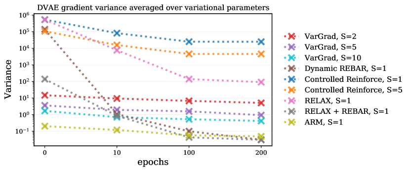
Refer to caption
Figure B.5: Estimates of the gradient variance of the DVAE at 4 points during the optimisation for different gradient estimators. The plot compares VarGrad to Reinforce with score function control variates [Ranganath et al., 2014], dynamic rebar [Tucker et al., 2017], relax, relax + rebar [Grathwohl et al., 2018] and ARM [Yin and Zhou, 2019]. The number of samples used to compute each gradient estimator is given in the figure legend.

B.3.2 Performance in Optimisation

In this section we present additional results on training the DVAE with VarGrad. Figure B.6 replicates Figure 4 with a longer run-time. Figure B.7 and Figure B.8 show the optimisation traces for different Adam learning rates.

Refer to caption
Figure B.6: Optimisation trace versus epoch (left) and wall-clock time (right) for a two-layer linear dvae on a fixed binarisation of Omniglot, trained with Adam with a learning rate of 0.001. The plot compares VarGrad to Reinforce with score function control variates [Ranganath et al., 2014], dynamic rebar [Tucker et al., 2017], relax, relax + rebar [Grathwohl et al., 2018] and ARM [Yin and Zhou, 2019]. The number of samples used to compute each gradient estimator is given in the figure legend. The results here are identical to the ones in Figure 4 but with a longer run-time.
Refer to caption
Figure B.7: Optimisation trace versus epoch (left) and wall-clock time (right) for a two-layer linear dvae on a fixed binarisation of Omniglot, trained with Adam with a learning rate of 0.0005. The plot compares VarGrad to Reinforce with score function control variates [Ranganath et al., 2014], dynamic rebar [Tucker et al., 2017], relax, relax + rebar [Grathwohl et al., 2018] and ARM [Yin and Zhou, 2019]. The number of samples used to compute each gradient estimator is given in the figure legend.
Refer to caption
Figure B.8: Optimisation trace versus epoch (left) and wall-clock time (right) for a two-layer linear dvae on a fixed binarisation of Omniglot, trained with Adam with a learning rate of 0.0001. The plot compares VarGrad to Reinforce with score function control variates [Ranganath et al., 2014], dynamic rebar [Tucker et al., 2017], relax, relax + rebar [Grathwohl et al., 2018] and ARM [Yin and Zhou, 2019]. The number of samples used to compute each gradient estimator is given in the figure legend.

Appendix C Gaussians

In the case when q(z)𝑞𝑧q(z) and p(z|x)𝑝conditional𝑧𝑥p(z|x) are (diagonal) Gaussians we can gain some intuition on the performance of VarGrad by computing the relevant quantities analytically. The principal insights obtained from the examples presented in this section can be summarised as follows: Firstly, in certain scenarios the Reinforce estimator does indeed exhibit a lower variance in comparison with VarGrad (although the advantage is very modest and only materialises for a restricted set of parameters). This finding illustrates that the conditions in Eq. 19 and Eq. 20 (the latter referring to SS0𝑆subscript𝑆0S\geq S_{0}) cannot be dropped without replacement from the formulation of Proposition 3. Secondly, in line with the results from Section 6, the relative error δiCV/𝔼[aVarGrad]superscriptsubscript𝛿𝑖CV𝔼delimited-[]superscript𝑎VarGrad\delta_{i}^{\textrm{CV}}/{\mathbb{E}}[a^{\textnormal{VarGrad}}] decreases with increased dimensionality. Moreover, the variance associated to computing the optimal control variate coefficients asuperscript𝑎a^{*} is significant and increases considerably with the number of latent variables.

C.1 Comparing the Variances of Reinforce and VarGrad

In order to understand when the variance of VarGrad is smaller than the variance of the Reinforce estimator we first consider the one-dimensional Gaussian case q(z)=𝒩(z;μ,σ2)𝑞𝑧𝒩𝑧𝜇superscript𝜎2q(z)=\mathcal{N}(z;\mu,\sigma^{2}) and p(z|x)=𝒩(z;μ~,σ~2)𝑝conditional𝑧𝑥𝒩𝑧~𝜇superscript~𝜎2p(z|x)=\mathcal{N}(z;\widetilde{\mu},\widetilde{\sigma}^{2}) and analyse the derivative w.r.t. μ𝜇\mu. A lengthy calculation shows that

ΔVarsubscriptΔVar\displaystyle\Delta_{\operatorname{Var}} (μ,μ~,σ2,σ~2,S):=Var(g^Reinforce,μ)Var(g^VarGrad,μ)assign𝜇~𝜇superscript𝜎2superscript~𝜎2𝑆Varsubscript^𝑔Reinforce𝜇Varsubscript^𝑔VarGrad𝜇\displaystyle(\mu,\widetilde{\mu},\sigma^{2},\widetilde{\sigma}^{2},S):=\operatorname{Var}(\widehat{g}_{\text{Reinforce},\mu})-\operatorname{Var}(\widehat{g}_{\text{VarGrad},\mu}) (46a)
=14Sσ4σ~2((μμ~)4+2(μμ~)2(3S7S1σ23σ~2)+5S7S1(σ2σ~2)2)absent14𝑆superscript𝜎4superscript~𝜎2superscript𝜇~𝜇42superscript𝜇~𝜇23𝑆7𝑆1superscript𝜎23superscript~𝜎25𝑆7𝑆1superscriptsuperscript𝜎2superscript~𝜎22\displaystyle=\frac{1}{4S{\sigma}^{4}\widetilde{\sigma}^{2}}\left((\mu-\widetilde{\mu})^{4}+2(\mu-\widetilde{\mu})^{2}\left(\frac{3S-7}{S-1}{\sigma}^{2}-3\widetilde{\sigma}^{2}\right)+\frac{5S-7}{S-1}\left({\sigma}^{2}-\widetilde{\sigma}^{2}\right)^{2}\right) (46b)
14Sσ4σ~2(Δμ4+6Δμ2Δσ2+5Δσ22),absent14𝑆superscript𝜎4superscript~𝜎2superscriptsubscriptΔ𝜇46superscriptsubscriptΔ𝜇2subscriptΔsuperscript𝜎25superscriptsubscriptΔsuperscript𝜎22\displaystyle\approx\frac{1}{4S{\sigma}^{4}\widetilde{\sigma}^{2}}\left(\Delta_{\mu}^{4}+6\Delta_{\mu}^{2}\Delta_{\sigma^{2}}+5\Delta_{\sigma^{2}}^{2}\right), (46c)

where the last line holds for large S𝑆S with Δμ:=μμ~assignsubscriptΔ𝜇𝜇~𝜇\Delta_{\mu}:=\mu-\widetilde{\mu} and Δσ2:=σ2σ~2assignsubscriptΔsuperscript𝜎2superscript𝜎2superscript~𝜎2\Delta_{\sigma^{2}}:={\sigma}^{2}-\widetilde{\sigma}^{2}.

For an illustration, let us vary the above parameters. First, let us fix σ2=σ~2=1superscript𝜎2superscript~𝜎21\sigma^{2}=\widetilde{\sigma}^{2}=1. We note from Eq. 46c that in this case we expect VarGrad to have lower variance regardless of ΔμsubscriptΔ𝜇\Delta_{\mu} as long as S𝑆S is large enough. In Figure C.9 we see that this is in fact the case, however a different result can be observed for small S𝑆S, which is again in accordance with Eq. 46b.
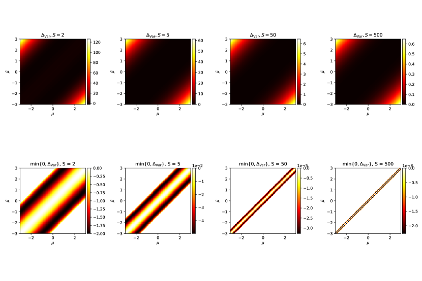
Refer to caption
Figure C.9: We compare the variance of the reinforce estimator with the variance of VarGrad. VarGrad is often better even for small S𝑆S – for large S𝑆S this can be guaranteed with Proposition 3.

Next, we consider arbitrary σ2superscript𝜎2\sigma^{2} and σ~2superscript~𝜎2\widetilde{\sigma}^{2}, but fixed μ=1,μ~=2formulae-sequence𝜇1~𝜇2\mu=1,\widetilde{\mu}=2. In Figure C.10 we observe that the variance of VarGrad is smaller for most values of σ2superscript𝜎2\sigma^{2} and σ~2superscript~𝜎2\widetilde{\sigma}^{2}. However, even for large S𝑆S there remains a region where the Reinforce estimator is superior. In fact, one can compute the condition for this to happen to be Δσ2[Δμ2,15Δμ2]subscriptΔsuperscript𝜎2superscriptsubscriptΔ𝜇215superscriptsubscriptΔ𝜇2\Delta_{\sigma^{2}}\in\left[-\Delta_{\mu}^{2},-\frac{1}{5}\Delta_{\mu}^{2}\right], which can be compared with the condition in Eq. 19 in Proposition 3.
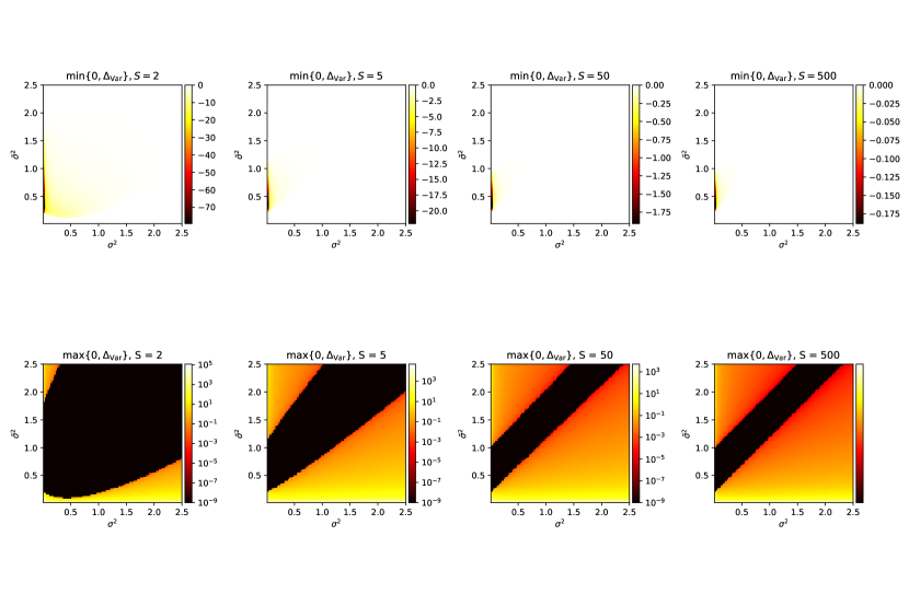
Refer to caption
Figure C.10: Variance comparison with varying σ2superscript𝜎2\sigma^{2} and σ~2superscript~𝜎2\widetilde{\sigma}^{2}. VarGrad only wins outside a certain region, however, if so, then potentially by orders of magnitude.

In Figure C.11 we display the variance differences ΔVarsubscriptΔVar\Delta_{\operatorname{Var}} as functions of ΔμsubscriptΔ𝜇\Delta_{\mu} and Δσ2subscriptΔsuperscript𝜎2\Delta_{\sigma^{2}}, approximated according to Eq. 46c, for the same fixed values as before and see that they are bounded from below, but not from above.
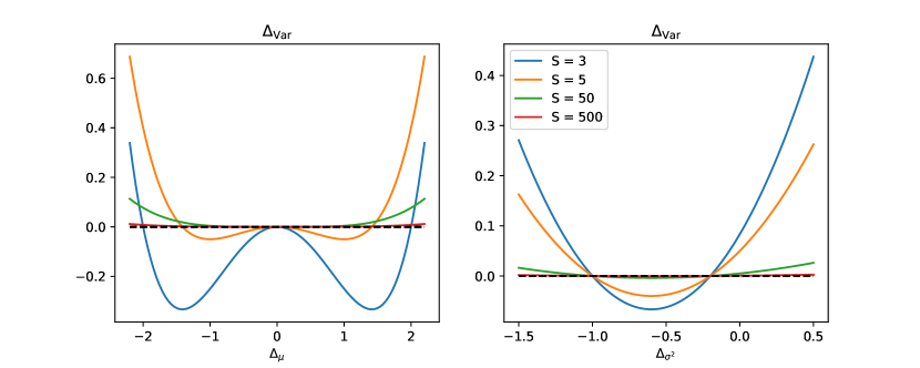
Refer to caption
Figure C.11: Variance differences of the reinforce estimator and VarGrad with varying ΔμsubscriptΔ𝜇\Delta_{\mu} and Δσ2subscriptΔsuperscript𝜎2\Delta_{\sigma^{2}} for different sample sizes S𝑆S.

For a D𝐷D-dimensional Gaussian it is hard to compute the condition from Eq. 19 in full generality, but we can derive the following stronger criterion that can guarantee better performance of VarGrad when assuming that ELBO(ϕ)0ELBOitalic-ϕ0\mathrm{ELBO}(\phi)\leq 0 (which for instance holds in the discrete-data setting).

Lemma 5.

Assume ELBO(ϕ)0ELBOitalic-ϕ0\mathrm{ELBO}(\phi)\leq 0 and

Cov(fϕ,(ϕilogqϕ)2)>0.Covsubscript𝑓italic-ϕsuperscriptsubscriptsubscriptitalic-ϕ𝑖subscript𝑞italic-ϕ20\operatorname{Cov}\left(f_{\phi},\left(\partial_{\phi_{i}}\log q_{\phi}\right)^{2}\right)>0. (47)

Then there exists S0subscript𝑆0S_{0}\in\mathbb{N} such that

Var(g^VarGrad,i(ϕ))Var(g^Reinforce,i(ϕ)),for allSS0.formulae-sequenceVarsubscript^𝑔VarGrad𝑖italic-ϕVarsubscript^𝑔Reinforce𝑖italic-ϕfor all𝑆subscript𝑆0\operatorname{Var}\left(\widehat{g}_{\text{VarGrad},i}(\phi)\right)\leq\operatorname{Var}\left(\widehat{g}_{\text{Reinforce},i}(\phi)\right),\quad\quad\textnormal{for all}\quad S\geq S_{0}. (48)
Proof.

With ELBO(ϕ)0ELBOitalic-ϕ0\mathrm{ELBO}(\phi)\leq 0 we have

Cov(fϕ,(ϕilogqϕ)2)Covsubscript𝑓italic-ϕsuperscriptsubscriptsubscriptitalic-ϕ𝑖subscript𝑞italic-ϕ2\displaystyle\operatorname{Cov}\left(f_{\phi},\left(\partial_{\phi_{i}}\log q_{\phi}\right)^{2}\right) 𝔼qϕ[fϕ(ϕilogqϕ)2]12𝔼qϕ[fϕ]𝔼qϕ[(ϕilogqϕ)2]absentsubscript𝔼subscript𝑞italic-ϕsubscript𝑓italic-ϕsuperscriptsubscriptsubscriptitalic-ϕ𝑖subscript𝑞italic-ϕ212subscript𝔼subscript𝑞italic-ϕsubscript𝑓italic-ϕsubscript𝔼subscript𝑞italic-ϕsuperscriptsubscriptsubscriptitalic-ϕ𝑖subscript𝑞italic-ϕ2\displaystyle\leq\operatorname{\mathbb{E}}_{q_{\phi}}\left[f_{\phi}\left(\partial_{\phi_{i}}\log q_{\phi}\right)^{2}\right]-\frac{1}{2}\operatorname{\mathbb{E}}_{q_{\phi}}\left[f_{\phi}\right]\operatorname{\mathbb{E}}_{q_{\phi}}\left[\left(\partial_{\phi_{i}}\log q_{\phi}\right)^{2}\right] (49)
=𝔼qϕ[(ϕilogqϕ)2](δiCV12ELBO(ϕ)).absentsubscript𝔼subscript𝑞italic-ϕsuperscriptsubscriptsubscriptitalic-ϕ𝑖subscript𝑞italic-ϕ2subscriptsuperscript𝛿CV𝑖12ELBOitalic-ϕ\displaystyle=\operatorname{\mathbb{E}}_{q_{\phi}}\left[\left(\partial_{\phi_{i}}\log q_{\phi}\right)^{2}\right]\left(\delta^{\text{CV}}_{i}-\frac{1}{2}\mathrm{ELBO}(\phi)\right). (50)

If now

Cov(fϕ,(ϕilogqϕ)2)>0,Covsubscript𝑓italic-ϕsuperscriptsubscriptsubscriptitalic-ϕ𝑖subscript𝑞italic-ϕ20\operatorname{Cov}\left(f_{\phi},\left(\partial_{\phi_{i}}\log q_{\phi}\right)^{2}\right)>0, (51)

then also

δiCV12ELBO(ϕ)>0,subscriptsuperscript𝛿CV𝑖12ELBOitalic-ϕ0\delta^{\text{CV}}_{i}-\frac{1}{2}\mathrm{ELBO}(\phi)>0, (52)

and the statement follows by Proposition 3. \Box

The condition from Eq. 47 gives another guarantee for VarGrad having smaller variance than the Reinforce estimator. However, we note that the converse statement is not necessarily true, i.e. if the condition does not hold, VarGrad can still be better. The advantage of Eq. 47, however, is that it can be verified more easily in certain settings, as for instance done for D𝐷D-dimensional diagonal Gaussians in the following lemma.

Lemma 6 (Covariance term for diagonal Gaussians).

Let q(z)𝑞𝑧q(z) and p(z|x)𝑝conditional𝑧𝑥p(z|x) be diagonal D𝐷D-dimensional Gaussians with means μ𝜇\mu and μ~~𝜇\widetilde{\mu} and covariance matrices Σ=diag(σ12,,σD2)Σdiagsuperscriptsubscript𝜎12superscriptsubscript𝜎𝐷2\Sigma=\operatorname{diag}(\sigma_{1}^{2},\dots,\sigma_{D}^{2}) and Σ~=diag(σ~12,,σ~D2)~Σdiagsuperscriptsubscript~𝜎12superscriptsubscript~𝜎𝐷2\widetilde{\Sigma}=\operatorname{diag}(\widetilde{\sigma}_{1}^{2},\dots,\widetilde{\sigma}_{D}^{2}). Then

Covqϕ(fϕ,(ϕklogqϕ)2)=1σ~k21σk2subscriptCovsubscript𝑞italic-ϕsubscript𝑓italic-ϕsuperscriptsubscriptsubscriptitalic-ϕ𝑘subscript𝑞italic-ϕ21superscriptsubscript~𝜎𝑘21superscriptsubscript𝜎𝑘2\operatorname{Cov}_{q_{\phi}}\left(f_{\phi},\left(\partial_{\phi_{k}}\log q_{\phi}\right)^{2}\right)=\frac{1}{\widetilde{\sigma}_{k}^{2}}-\frac{1}{\sigma_{k}^{2}} (53)

for k{1,,D}𝑘1𝐷k\in\{1,\dots,D\} and

Covqϕ(fϕ,(ϕklogqϕ)2)=1σk2(1σ~k21σk2)subscriptCovsubscript𝑞italic-ϕsubscript𝑓italic-ϕsuperscriptsubscriptsubscriptitalic-ϕ𝑘subscript𝑞italic-ϕ21superscriptsubscript𝜎𝑘21superscriptsubscript~𝜎𝑘21superscriptsubscript𝜎𝑘2\operatorname{Cov}_{q_{\phi}}\left(f_{\phi},\left(\partial_{\phi_{k}}\log q_{\phi}\right)^{2}\right)=\frac{1}{{\sigma}_{k}^{2}}\left(\frac{1}{\widetilde{\sigma}_{k}^{2}}-\frac{1}{{\sigma}_{k}^{2}}\right) (54)

for k{D+1,,2D}𝑘𝐷12𝐷k\in\{D+1,\dots,2D\} with ϕ=(μ1,,μD,σ12,,σD2)italic-ϕsuperscriptsubscript𝜇1subscript𝜇𝐷superscriptsubscript𝜎12superscriptsubscript𝜎𝐷2top\phi=(\mu_{1},\dots,\mu_{D},\sigma_{1}^{2},\dots,\sigma_{D}^{2})^{\top} and

Covqϕ(fϕ,(ϕklogqϕ)2)=1σ~k21σk2subscriptCovsubscript𝑞italic-ϕsubscript𝑓italic-ϕsuperscriptsubscriptsubscriptitalic-ϕ𝑘subscript𝑞italic-ϕ21superscriptsubscript~𝜎𝑘21superscriptsubscript𝜎𝑘2\operatorname{Cov}_{q_{\phi}}\left(f_{\phi},\left(\partial_{\phi_{k}}\log q_{\phi}\right)^{2}\right)=\frac{1}{\widetilde{\sigma}_{k}^{2}}-\frac{1}{{\sigma}_{k}^{2}} (55)

for k{D+1,,2D}𝑘𝐷12𝐷k\in\{D+1,\dots,2D\} with ϕ=(μ1,,μD,logσ12,,logσD2)italic-ϕsuperscriptsubscript𝜇1subscript𝜇𝐷superscriptsubscript𝜎12superscriptsubscript𝜎𝐷2top\phi=(\mu_{1},\dots,\mu_{D},\log\sigma_{1}^{2},\dots,\log\sigma_{D}^{2})^{\top}.

Proof.

We compute

fϕ=12i=1Dlog(σi2σ~i2)12i=1D(ziμi)2σi2+12i=1D(ziμ~i)2σ~i2subscript𝑓italic-ϕ12superscriptsubscript𝑖1𝐷superscriptsubscript𝜎𝑖2superscriptsubscript~𝜎𝑖212superscriptsubscript𝑖1𝐷superscriptsubscript𝑧𝑖subscript𝜇𝑖2superscriptsubscript𝜎𝑖212superscriptsubscript𝑖1𝐷superscriptsubscript𝑧𝑖subscript~𝜇𝑖2subscriptsuperscript~𝜎2𝑖f_{\phi}=-\frac{1}{2}\sum_{i=1}^{D}\log\left(\frac{\sigma_{i}^{2}}{\widetilde{\sigma}_{i}^{2}}\right)-\frac{1}{2}\sum_{i=1}^{D}\frac{(z_{i}-\mu_{i})^{2}}{\sigma_{i}^{2}}+\frac{1}{2}\sum_{i=1}^{D}\frac{(z_{i}-\widetilde{\mu}_{i})^{2}}{\widetilde{\sigma}^{2}_{i}} (56)

and

μklogqϕ=zkμkσk2.subscriptsubscript𝜇𝑘subscript𝑞italic-ϕsubscript𝑧𝑘subscript𝜇𝑘superscriptsubscript𝜎𝑘2\partial_{\mu_{k}}\log q_{\phi}=\frac{z_{k}-\mu_{k}}{\sigma_{k}^{2}}. (57)

We again use the short-cuts

A=fϕ(z),B=(μklogqϕ)(z),formulae-sequence𝐴subscript𝑓italic-ϕ𝑧𝐵subscriptsubscript𝜇𝑘subscript𝑞italic-ϕ𝑧A=f_{\phi}(z),\qquad B=\left(\partial_{\mu_{k}}\log q_{\phi}\right)(z), (58)

and obtain

Covqϕ(A,B2)=𝔼qϕ[AB2]𝔼qϕ[A]𝔼qϕ[B2]subscriptCovsubscript𝑞italic-ϕ𝐴superscript𝐵2subscript𝔼subscript𝑞italic-ϕ𝐴superscript𝐵2subscript𝔼subscript𝑞italic-ϕ𝐴subscript𝔼subscript𝑞italic-ϕsuperscript𝐵2\displaystyle\operatorname{Cov}_{q_{\phi}}(A,B^{2})=\operatorname{\mathbb{E}}_{q_{\phi}}\left[AB^{2}\right]-\operatorname{\mathbb{E}}_{q_{\phi}}[A]\operatorname{\mathbb{E}}_{q_{\phi}}\left[B^{2}\right] (59)
=𝔼qϕ[(12i=1Dlog(σi2σ~i2)12i=1D(ziμi)2σi2+12i=1D(ziμ~i)2σ~i2)(zkμkσk2)2]absentsubscript𝔼subscript𝑞italic-ϕ12superscriptsubscript𝑖1𝐷superscriptsubscript𝜎𝑖2superscriptsubscript~𝜎𝑖212superscriptsubscript𝑖1𝐷superscriptsubscript𝑧𝑖subscript𝜇𝑖2superscriptsubscript𝜎𝑖212superscriptsubscript𝑖1𝐷superscriptsubscript𝑧𝑖subscript~𝜇𝑖2subscriptsuperscript~𝜎2𝑖superscriptsubscript𝑧𝑘subscript𝜇𝑘superscriptsubscript𝜎𝑘22\displaystyle=\operatorname{\mathbb{E}}_{q_{\phi}}\left[\left(-\frac{1}{2}\sum_{i=1}^{D}\log\left(\frac{\sigma_{i}^{2}}{\widetilde{\sigma}_{i}^{2}}\right)-\frac{1}{2}\sum_{i=1}^{D}\frac{(z_{i}-\mu_{i})^{2}}{\sigma_{i}^{2}}+\frac{1}{2}\sum_{i=1}^{D}\frac{(z_{i}-\widetilde{\mu}_{i})^{2}}{\widetilde{\sigma}^{2}_{i}}\right)\left(\frac{z_{k}-\mu_{k}}{\sigma_{k}^{2}}\right)^{2}\right] (60)
𝔼qϕ[(12i=1Dlog(σi2σ~i2)12i=1D(ziμi)2σi2+12i=1D(ziμ~i)2σ~i2)]𝔼qϕ[(zkμkσk2)2]subscript𝔼subscript𝑞italic-ϕ12superscriptsubscript𝑖1𝐷superscriptsubscript𝜎𝑖2superscriptsubscript~𝜎𝑖212superscriptsubscript𝑖1𝐷superscriptsubscript𝑧𝑖subscript𝜇𝑖2superscriptsubscript𝜎𝑖212superscriptsubscript𝑖1𝐷superscriptsubscript𝑧𝑖subscript~𝜇𝑖2subscriptsuperscript~𝜎2𝑖subscript𝔼subscript𝑞italic-ϕsuperscriptsubscript𝑧𝑘subscript𝜇𝑘superscriptsubscript𝜎𝑘22\displaystyle\quad-\operatorname{\mathbb{E}}_{q_{\phi}}\left[\left(-\frac{1}{2}\sum_{i=1}^{D}\log\left(\frac{\sigma_{i}^{2}}{\widetilde{\sigma}_{i}^{2}}\right)-\frac{1}{2}\sum_{i=1}^{D}\frac{(z_{i}-\mu_{i})^{2}}{\sigma_{i}^{2}}+\frac{1}{2}\sum_{i=1}^{D}\frac{(z_{i}-\widetilde{\mu}_{i})^{2}}{\widetilde{\sigma}^{2}_{i}}\right)\right]\operatorname{\mathbb{E}}_{q_{\phi}}\left[\left(\frac{z_{k}-\mu_{k}}{\sigma_{k}^{2}}\right)^{2}\right] (61)
=12(3σk2+D1σk2)+12(1σk2i=1ikDσi2+(μiμ~i)2σ~i2+1σk2σ~k2(3σk2+(μkμ~k)2))absent123superscriptsubscript𝜎𝑘2𝐷1superscriptsubscript𝜎𝑘2121superscriptsubscript𝜎𝑘2superscriptsubscript𝑖1𝑖𝑘𝐷superscriptsubscript𝜎𝑖2superscriptsubscript𝜇𝑖subscript~𝜇𝑖2superscriptsubscript~𝜎𝑖21superscriptsubscript𝜎𝑘2superscriptsubscript~𝜎𝑘23superscriptsubscript𝜎𝑘2superscriptsubscript𝜇𝑘subscript~𝜇𝑘2\displaystyle=-\frac{1}{2}\left(\frac{3}{\sigma_{k}^{2}}+\frac{D-1}{\sigma_{k}^{2}}\right)+\frac{1}{2}\left(\frac{1}{{\sigma}_{k}^{2}}\sum_{\begin{subarray}{c}i=1\\ i\neq k\end{subarray}}^{D}\frac{\sigma_{i}^{2}+(\mu_{i}-\widetilde{\mu}_{i})^{2}}{\widetilde{\sigma}_{i}^{2}}+\frac{1}{\sigma_{k}^{2}\widetilde{\sigma}_{k}^{2}}\left(3\sigma_{k}^{2}+(\mu_{k}-\widetilde{\mu}_{k})^{2}\right)\right) (62)
(D2+12i=1Dσi2+(μiμ~i)2σ~i2)1σk2𝐷212superscriptsubscript𝑖1𝐷superscriptsubscript𝜎𝑖2superscriptsubscript𝜇𝑖subscript~𝜇𝑖2superscriptsubscript~𝜎𝑖21superscriptsubscript𝜎𝑘2\displaystyle\quad-\left(-\frac{D}{2}+\frac{1}{2}\sum_{i=1}^{D}\frac{\sigma_{i}^{2}+(\mu_{i}-\widetilde{\mu}_{i})^{2}}{\widetilde{\sigma}_{i}^{2}}\right)\frac{1}{\sigma_{k}^{2}} (63)
=1σk2+12σk2σ~k2(3σk2+(μμ~)2)12σk2σ~k2(σk2+(μμ~)2)absent1superscriptsubscript𝜎𝑘212superscriptsubscript𝜎𝑘2superscriptsubscript~𝜎𝑘23superscriptsubscript𝜎𝑘2superscript𝜇~𝜇212superscriptsubscript𝜎𝑘2superscriptsubscript~𝜎𝑘2superscriptsubscript𝜎𝑘2superscript𝜇~𝜇2\displaystyle=-\frac{1}{\sigma_{k}^{2}}+\frac{1}{2\sigma_{k}^{2}\widetilde{\sigma}_{k}^{2}}\left(3\sigma_{k}^{2}+(\mu-\widetilde{\mu})^{2}\right)-\frac{1}{2\sigma_{k}^{2}\widetilde{\sigma}_{k}^{2}}\left(\sigma_{k}^{2}+(\mu-\widetilde{\mu})^{2}\right) (64)
=1σ~k21σk2.absent1superscriptsubscript~𝜎𝑘21superscriptsubscript𝜎𝑘2\displaystyle=\frac{1}{\widetilde{\sigma}_{k}^{2}}-\frac{1}{\sigma_{k}^{2}}. (65)

For the terms with the partial derivative w.r.t. σk2superscriptsubscript𝜎𝑘2\sigma_{k}^{2} we first note that

σk2logqϕ=12σk2+(zkμk)22σk4=1σk2logσk2logqϕ.subscriptsuperscriptsubscript𝜎𝑘2subscript𝑞italic-ϕ12superscriptsubscript𝜎𝑘2superscriptsubscript𝑧𝑘subscript𝜇𝑘22superscriptsubscript𝜎𝑘41superscriptsubscript𝜎𝑘2subscriptsuperscriptsubscript𝜎𝑘2subscript𝑞italic-ϕ\partial_{\sigma_{k}^{2}}\log q_{\phi}=-\frac{1}{2\sigma_{k}^{2}}+\frac{(z_{k}-\mu_{k})^{2}}{2\sigma_{k}^{4}}=\frac{1}{\sigma_{k}^{2}}\partial_{\log\sigma_{k}^{2}}\log q_{\phi}. (66)

We compute

𝔼qϕ[AB2]subscript𝔼subscript𝑞italic-ϕ𝐴superscript𝐵2\displaystyle\operatorname{\mathbb{E}}_{q_{\phi}}\left[AB^{2}\right] =𝔼qϕ[(zkμk)24σk6i=1D(ziμi)2σi2(zkμk)48σk8i=1D(ziμi)2σi2\displaystyle=\operatorname{\mathbb{E}}_{q_{\phi}}\Bigg{[}\frac{(z_{k}-\mu_{k})^{2}}{4\sigma_{k}^{6}}\sum_{i=1}^{D}\frac{(z_{i}-\mu_{i})^{2}}{\sigma_{i}^{2}}-\frac{(z_{k}-\mu_{k})^{4}}{8\sigma_{k}^{8}}\sum_{i=1}^{D}\frac{(z_{i}-\mu_{i})^{2}}{\sigma_{i}^{2}} (67)
(zkμk)24σk6i=1D(ziμ~i)2σ~i2+(zkμk)48σk8i=1D(ziμ~i)2σ~i2]\displaystyle\quad\quad\qquad-\frac{(z_{k}-\mu_{k})^{2}}{4\sigma_{k}^{6}}\sum_{i=1}^{D}\frac{(z_{i}-\widetilde{\mu}_{i})^{2}}{\widetilde{\sigma}_{i}^{2}}+\frac{(z_{k}-\mu_{k})^{4}}{8\sigma_{k}^{8}}\sum_{i=1}^{D}\frac{(z_{i}-\widetilde{\mu}_{i})^{2}}{\widetilde{\sigma}_{i}^{2}}\Bigg{]} (68)
=18σk4(D+8)+18σk4σ~k2(9σk2+(μkμ~k)2)+18σk4i=1ikdσi2+(μiμi~)2σ~i2,absent18superscriptsubscript𝜎𝑘4𝐷818superscriptsubscript𝜎𝑘4superscriptsubscript~𝜎𝑘29superscriptsubscript𝜎𝑘2superscriptsubscript𝜇𝑘subscript~𝜇𝑘218superscriptsubscript𝜎𝑘4superscriptsubscript𝑖1𝑖𝑘𝑑superscriptsubscript𝜎𝑖2superscriptsubscript𝜇𝑖~subscript𝜇𝑖2superscriptsubscript~𝜎𝑖2\displaystyle=-\frac{1}{8\sigma_{k}^{4}}(D+8)+\frac{1}{8\sigma_{k}^{4}\widetilde{\sigma}_{k}^{2}}(9\sigma_{k}^{2}+(\mu_{k}-\widetilde{\mu}_{k})^{2})+\frac{1}{8\sigma_{k}^{4}}\sum_{\begin{subarray}{c}i=1\\ i\neq k\end{subarray}}^{d}\frac{\sigma_{i}^{2}+(\mu_{i}-\widetilde{\mu_{i}})^{2}}{\widetilde{\sigma}_{i}^{2}}, (69)

and similarly

𝔼qϕ[A]𝔼qϕ[B2]=D8σk4+18σk4σ~k2(σk2+(μkμ~k)2)+18σk4i=1ikDσi2+(μiμ~i)2σ~i2.subscript𝔼subscript𝑞italic-ϕ𝐴subscript𝔼subscript𝑞italic-ϕsuperscript𝐵2𝐷8superscriptsubscript𝜎𝑘418superscriptsubscript𝜎𝑘4superscriptsubscript~𝜎𝑘2superscriptsubscript𝜎𝑘2superscriptsubscript𝜇𝑘subscript~𝜇𝑘218superscriptsubscript𝜎𝑘4superscriptsubscript𝑖1𝑖𝑘𝐷superscriptsubscript𝜎𝑖2superscriptsubscript𝜇𝑖subscript~𝜇𝑖2superscriptsubscript~𝜎𝑖2\displaystyle\operatorname{\mathbb{E}}_{q_{\phi}}[A]\operatorname{\mathbb{E}}_{q_{\phi}}\left[B^{2}\right]=-\frac{D}{8\sigma_{k}^{4}}+\frac{1}{8\sigma_{k}^{4}\widetilde{\sigma}_{k}^{2}}\left(\sigma_{k}^{2}+(\mu_{k}-\widetilde{\mu}_{k})^{2}\right)+\frac{1}{8\sigma_{k}^{4}}\sum_{\begin{subarray}{c}i=1\\ i\neq k\end{subarray}}^{D}\frac{\sigma_{i}^{2}+(\mu_{i}-\widetilde{\mu}_{i})^{2}}{\widetilde{\sigma}_{i}^{2}}. (70)

We therefore get the result by again computing Covqϕ(A,B2)=𝔼qϕ[AB2]𝔼qϕ[A]𝔼qϕ[B2]subscriptCovsubscript𝑞italic-ϕ𝐴superscript𝐵2subscript𝔼subscript𝑞italic-ϕ𝐴superscript𝐵2subscript𝔼subscript𝑞italic-ϕ𝐴subscript𝔼subscript𝑞italic-ϕsuperscript𝐵2\operatorname{Cov}_{q_{\phi}}(A,B^{2})=\operatorname{\mathbb{E}}_{q_{\phi}}\left[AB^{2}\right]-\operatorname{\mathbb{E}}_{q_{\phi}}[A]\operatorname{\mathbb{E}}_{q_{\phi}}\left[B^{2}\right]. The partial derivative w.r.t. logσk2superscriptsubscript𝜎𝑘2\log\sigma_{k}^{2} can be recovered from Eq. 66. \Box

C.2 Optimal Control Variates in the Gaussian Case

In the diagonal Gaussian case we can also easily analytically compute the optimal control variate coefficients from Eq. 11, along the lines of the proof of Lemma 6. Our setting is again q(z)=𝒩(z;μ,Σ)𝑞𝑧𝒩𝑧𝜇Σq(z)=\mathcal{N}(z;\mu,\Sigma), p(z|x)=𝒩(z;μ~,Σ~)𝑝conditional𝑧𝑥𝒩𝑧~𝜇~Σp(z|x)=\mathcal{N}(z;\widetilde{\mu},\widetilde{\Sigma}) with Σ=diag(σ12,,σD2)Σdiagsuperscriptsubscript𝜎12superscriptsubscript𝜎𝐷2\Sigma=\operatorname{diag}\left(\sigma_{1}^{2},\dots,\sigma_{D}^{2}\right), Σ~=diag(σ~12,,σ~D2)~Σdiagsuperscriptsubscript~𝜎12superscriptsubscript~𝜎𝐷2\widetilde{\Sigma}=\operatorname{diag}\left(\widetilde{\sigma}_{1}^{2},\dots,\widetilde{\sigma}_{D}^{2}\right). In Figure C.12 we plot the variances of four different gradient estimators with varying sample size S𝑆S, namely g^Reinforcesubscript^𝑔Reinforce\widehat{g}_{\text{Reinforce}}, g^VarGradsubscript^𝑔VarGrad\widehat{g}_{\text{VarGrad}}, as well as the Reinforce estimator augmented with the optimal control variate, once computed analytically and once sampled using S𝑆S samples. The variance depends on the mean and the covariance matrix; here we choose μi=3subscript𝜇𝑖3\mu_{i}=3, σi2=3superscriptsubscript𝜎𝑖23\sigma_{i}^{2}=3, μ~i=1subscript~𝜇𝑖1\widetilde{\mu}_{i}=1, σ~i2=1superscriptsubscript~𝜎𝑖21\widetilde{\sigma}_{i}^{2}=1 for all i{1,,D}𝑖1𝐷i\in\{1,\dots,D\}.

Refer to caption
Figure C.12: Comparion of the variances of the different gradient estimators g^Reinforcesubscript^𝑔Reinforce\widehat{g}_{\text{Reinforce}}, g^VarGradsubscript^𝑔VarGrad\widehat{g}_{\text{VarGrad}}, as well as the reinforce estimator with the optimal control variate coefficient, once computed analytically and once sampled with S𝑆S samples, for dimensions D=3𝐷3D=3 and D=30𝐷30D=30.

We observe that the VarGrad estimator is close to the analyitcal optimal control variate, and that the sampled optimal control variate performs significantly worse in a small sample size regime. These observations get more pronounced in higher dimensions and indicate that the variance of the sampled optimal control variate can itself be high, showing that using it might not always be beneficial in practice.

Let us additionally investigate the optimal control variate correction term δiCVsuperscriptsubscript𝛿𝑖CV\delta_{i}^{\text{CV}} as defined in Eq. 13 for D𝐷D-dimensional Gaussians q(z)𝑞𝑧q(z) and p(z|x)𝑝conditional𝑧𝑥p(z|x) as considered above. In Figure C.13 we display the variances, means and relative errors of δiCVsuperscriptsubscript𝛿𝑖CV\delta_{i}^{\text{CV}} and aVarGrad=f¯ϕsuperscript𝑎VarGradsubscript¯𝑓italic-ϕa^{\text{VarGrad}}=\bar{f}_{\phi} and realise that indeed the ratio of those two converges to zero when D𝐷D gets larger. Furthermore we notice that the relative error of δCVsuperscript𝛿CV\delta^{\text{CV}} increases with the dimension, explaining the difficulties when estimating the optimal control variate coefficients from samples. Finally, we plot a histogramm of δiCVsubscriptsuperscript𝛿CV𝑖\delta^{\text{CV}}_{i} (varying across i𝑖i) in Figure C.14, showing that δiCVsubscriptsuperscript𝛿CV𝑖\delta^{\text{CV}}_{i} is small in comparison to 𝔼[aVarGrad]𝔼superscript𝑎VarGrad\operatorname{\mathbb{E}}\left[a^{\text{VarGrad}}\right] and distributed around zero.

Refer to caption
Figure C.13: Mean, variance and relative errors associated to the two contributions to the optimal control variate coefficient, δiCVsuperscriptsubscript𝛿𝑖CV\delta_{i}^{\text{CV}} and aVarGrad=f¯ϕsuperscript𝑎VarGradsubscript¯𝑓italic-ϕa^{\text{VarGrad}}=\bar{f}_{\phi}.
Refer to caption
Figure C.14: The histogram of δiCVsuperscriptsubscript𝛿𝑖CV\delta_{i}^{\text{CV}} shows that it is usually rather small in comparison to 𝔼[aVarGrad]𝔼superscript𝑎VarGrad\operatorname{\mathbb{E}}\left[a^{\text{VarGrad}}\right], which is roughly 700700700 here, and that it fluctuates around zero.

Appendix D Connections to Other Divergences

The Reinforce gradient estimator from Eq. 2 can as well be derived from the moment loss

rmoment(qϕ(z)p(z|x))=12𝔼r(z)[log2(qϕ(z)p(z|x))],\mathcal{L}_{r}^{\text{moment}}(q_{\phi}(z)\|p(z|x))=\frac{1}{2}\operatorname{\mathbb{E}}_{r(z)}\left[\log^{2}\left(\frac{q_{\phi}(z)}{p(z|x)}\right)\right], (71)

namely

ϕrmoment(qϕ(z)p(z|x))|r=qϕ=𝔼qϕ[log(qϕ(z)p(z|x))ϕlogqϕ(z)].\nabla_{\phi}\mathcal{L}_{r}^{\text{moment}}(q_{\phi}(z)\|p(z|x))\Big{|}_{r={q_{\phi}}}=\operatorname{\mathbb{E}}_{q_{\phi}}\left[\log\left(\frac{q_{\phi}(z)}{p(z|x)}\right)\nabla_{\phi}\log q_{\phi}(z)\right]. (72)

In the log-variance loss, one can omit the logarithm to obtain the variance loss

rVar(p(z|x)qϕ(z))=12Varr(z)(p(z|x)qϕ(z))=12𝔼r(z)[(p(z|x)qϕ(z))21],superscriptsubscript𝑟Varconditional𝑝conditional𝑧𝑥subscript𝑞italic-ϕ𝑧12subscriptVar𝑟𝑧𝑝conditional𝑧𝑥subscript𝑞italic-ϕ𝑧12subscript𝔼𝑟𝑧superscript𝑝conditional𝑧𝑥subscript𝑞italic-ϕ𝑧21\mathcal{L}_{r}^{\operatorname{Var}}(p(z|x)\|q_{\phi}(z))=\frac{1}{2}\operatorname{Var}_{r(z)}\left(\frac{p(z|x)}{q_{\phi}(z)}\right)=\frac{1}{2}\operatorname{\mathbb{E}}_{r(z)}\left[\left(\frac{p(z|x)}{q_{\phi}(z)}\right)^{2}-1\right], (73)

which with r=qϕ𝑟subscript𝑞italic-ϕr=q_{\phi} coincides with the χ2superscript𝜒2\chi^{2}-divergence. The potential of using the latter in the context of variational inference was suggested in Dieng et al. [2017]. We note that again one is in principle free in choosing r(z)𝑟𝑧r(z), but that unlike the log-variance loss, this loss in not symmetric with respect to qϕ(z)subscript𝑞italic-ϕ𝑧q_{\phi}(z) and p(z|x)𝑝conditional𝑧𝑥p(z|x). An analysis in Nüsken and Richter [2020] (for distributions on path space) however suggests that the variance loss (unlike the log-variance loss) scales unfavourably in high-dimensional settings in terms of the variance associated to standard Monte Carlo estimators.