Heat rectification with a minimal model of two harmonic oscillators

M. A. Simón miguelangel.simon@ehu.eus Departamento de Química-Física, Universidad del País Vasco, UPV- EHU - Bilbao, Spain    A. Alaña Departamento de Química-Física, Universidad del País Vasco, UPV- EHU - Bilbao, Spain    M. Pons Departamento de Física Aplicada I, Universidad del País Vasco, UPV- EHU - Bilbao, Spain    A. Ruiz-García Departamento de Física, Universidad de La Laguna, La Laguna 38203, Spain IUdEA Instituto Universitario de Estudios Avanzados, Universidad de La Laguna, La Laguna 38203, Spain    J. G. Muga jg.muga@ehu.es Departamento de Química-Física, Universidad del País Vasco, UPV- EHU - Bilbao, Spain
Abstract

We study heat rectification in a minimalistic model composed of two masses subjected to on-site and coupling linear forces in contact with effective Langevin baths induced by laser interactions. Analytic expressions of the heat currents in the steady state are spelled out. Asymmetric heat transport is found in this linear system if both the bath temperatures and the temperature dependent bath-system couplings are also exchanged.

I Introduction

Heat rectification, firstly observed in 1936 by Starr Starr (1936), is the physical phenomenon, analogous to electrical current rectification in diodes, in which heat current through a device or medium is not symmetric with respect to the exchange of the baths at the boundaries. In the limiting case the device allows heat to propagate in one direction from the hot to the cold bath while it behaves as a thermal insulator in the opposite direction when the baths are exchanged. In 2002 a paper by Terraneo et al. Terraneo et al. (2002) demonstrated heat rectification numerically for a chain of nonlinear oscillators in contact with two thermal baths at different temperatures. Since then, there has been a growing interest in heat rectification Pereira (2019); Roberts and Walker (2011); Li et al. (2012); Ye and Cao (2017); Wang and Li (2008, 2007); Li et al. (2006); Joulain et al. (2016); Chang et al. (2006); Kobayashi et al. (2009); Leitner (2013); Elzouka and Ndao (2017); Pons et al. (2017); Alexander (2020), and the field remains very active because of the potential applications in fundamental science and technology, and the fact that none of the proposals so far appears to be efficient and robust for practical purposes.

Much effort has been devoted to understand the underlying physical mechanism responsible for rectification Pereira (2019). In early times some kind of anharmonicity, i.e. non-linear forces, in the substrate potential or in the particle-particle interactions, was identified as a fundamental requisite for rectification Li et al. (2012, 2008); Hu et al. (2006); Zeng and Wang (2008); Katz and Kosloff (2016); Benenti et al. (2016). This non-harmonic behavior leads to a temperature dependence of the phonon bands. The match/mismatch of the phonon bands (power spectra) governs the heat transport in the chain, allowing it when the bands match or obstructing it if they mismatch Terraneo et al. (2002); Li et al. (2004). However, a work by Pereira et al. Pereira (2017) showed that rectification can also be found in effective harmonic systems if two requirements are met: some kind of structural asymmetry, and features that depend on the temperature so they change as the baths are inverted. Indeed, in this article we demonstrate rectification in a minimalistic model of two harmonic oscillators where the coupling to the baths depends on the temperature. This will be justified with a particular physical set up with trapped ions and lasers.

The article is organized as follows. In Section II we describe the physical model and its dynamical equations. In Section III we describe the dynamics of the system in terms of a covariance matrix. We also derive a set of algebraic equations that gives as solution the covariance matrix in the steady state. In Section IV we solve the covariance matrix equations and find analytical expressions for the steady-state temperatures of the masses and heat currents. In Section V we relate the parameters of our model to those in a physical set-up of Doppler cooled trapped ions. In Section VI we make a parameter sweep looking for configurations which yield high rectification. We also study the power spectra of the oscillators, which confirm the match/mismatch patterns in cases where there is rectification. In Section VII we summarize our results and present our conclusions.
Refer to caption
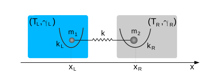
Figure 1: Diagram of the model described in Section II. Two ions coupled to each other through a spring constant k𝑘k. Each ion is harmonically trapped and connected to a bath characterized by its temperature Tisubscript𝑇𝑖T_{i} and its friction coefficient γisubscript𝛾𝑖\gamma_{i}.

II Physical Model

The physical model consists of two masses m1subscript𝑚1m_{1} and m2subscript𝑚2m_{2} coupled to each other by a harmonic interaction with spring constant k𝑘k and natural length xesubscript𝑥𝑒x_{e}. Each of the masses m1subscript𝑚1m_{1} and m2subscript𝑚2m_{2} are confined by a harmonic potential with spring constants kLsubscript𝑘𝐿k_{L}, kRsubscript𝑘𝑅k_{R} and equilibrium positions xLsubscript𝑥𝐿x_{L}, xRsubscript𝑥𝑅x_{R} respectively (see Fig. 1). The Hamiltonian describing this model is

H=p122m1+p222m2+V(x1,x2),𝐻superscriptsubscript𝑝122subscript𝑚1superscriptsubscript𝑝222subscript𝑚2𝑉subscript𝑥1subscript𝑥2H=\frac{p_{1}^{2}}{2m_{1}}+\frac{p_{2}^{2}}{2m_{2}}+V(x_{1},x_{2}), (1)

with V(x1,x2)=k2(x1x2xe)2+kL2(x1xL)2+kR2(x2xR)2𝑉subscript𝑥1subscript𝑥2𝑘2superscriptsubscript𝑥1subscript𝑥2subscript𝑥𝑒2subscript𝑘𝐿2superscriptsubscript𝑥1subscript𝑥𝐿2subscript𝑘𝑅2superscriptsubscript𝑥2subscript𝑥𝑅2V(x_{1},x_{2})=\frac{k}{2}\left(x_{1}-x_{2}-x_{e}\right)^{2}+\frac{k_{L}}{2}\left(x_{1}-x_{L}\right)^{2}+\frac{k_{R}}{2}\left(x_{2}-x_{R}\right)^{2}, where {xi,pi}i=1,2subscriptsubscript𝑥𝑖subscript𝑝𝑖𝑖12\{x_{i},p_{i}\}_{i=1,2} are the position and momentum of each mass. Switching from the original coordinates xisubscript𝑥𝑖x_{i} to displacements with respect to the equilibrium positions of the system qi=xixieqsubscript𝑞𝑖subscript𝑥𝑖superscriptsubscript𝑥𝑖𝑒𝑞q_{i}=x_{i}-x_{i}^{eq}, where xieqsuperscriptsubscript𝑥𝑖𝑒𝑞x_{i}^{eq} are the solutions to xiV(x1,x2)=0subscriptsubscript𝑥𝑖𝑉subscript𝑥1subscript𝑥20\partial_{x_{i}}V(x_{1},x_{2})=0, the Hamiltonian can be written as

H𝐻\displaystyle H =p122m1+p222m2+k+kL2q12absentsuperscriptsubscript𝑝122subscript𝑚1superscriptsubscript𝑝222subscript𝑚2𝑘subscript𝑘𝐿2superscriptsubscript𝑞12\displaystyle=\frac{p_{1}^{2}}{2m_{1}}+\frac{p_{2}^{2}}{2m_{2}}+\frac{k+k_{L}}{2}q_{1}^{2}
+k+kR2q22kq1q2+V(x1eq,x2eq).𝑘subscript𝑘𝑅2superscriptsubscript𝑞22𝑘subscript𝑞1subscript𝑞2𝑉superscriptsubscript𝑥1𝑒𝑞superscriptsubscript𝑥2𝑒𝑞\displaystyle+\frac{k+k_{R}}{2}q_{2}^{2}-kq_{1}q_{2}+V(x_{1}^{eq},x_{2}^{eq}). (2)

This has the form of the Hamiltonian of a system around a stable equilibrium point

H=12p𝖳𝕄1p+12q𝖳𝕂q,𝐻12superscript𝑝𝖳superscript𝕄1𝑝12superscript𝑞𝖳𝕂𝑞H=\frac{1}{2}\overrightarrow{p}^{\mathsf{T}}\mathbb{M}^{-1}\overrightarrow{p}+\frac{1}{2}\overrightarrow{q}^{\mathsf{T}}\mathbb{K}\overrightarrow{q}, (3)

where q=(q1,q2)𝖳𝑞superscriptsubscript𝑞1subscript𝑞2𝖳\overrightarrow{q}=\left(q_{1},q_{2}\right)^{\mathsf{T}}, p=(p1,p2)𝖳𝑝superscriptsubscript𝑝1subscript𝑝2𝖳\overrightarrow{p}=\left(p_{1},p_{2}\right)^{\mathsf{T}}, 𝕄=diag(m1,m2)𝕄𝑑𝑖𝑎𝑔subscript𝑚1subscript𝑚2\mathbb{M}=diag(m_{1},m_{2}) is the mass matrix of the system and 𝕂𝕂\mathbb{K} is the Hessian matrix of the potential at the equilibrium point, i.e., 𝕂ij=xi,xj2V(x)|x=xeqsubscript𝕂𝑖𝑗evaluated-atsubscriptsuperscript2subscript𝑥𝑖subscript𝑥𝑗𝑉𝑥𝑥superscript𝑥𝑒𝑞\mathbb{K}_{ij}=\partial^{2}_{x_{i},x_{j}}V(\overrightarrow{x})\Big{|}_{\overrightarrow{x}=\overrightarrow{x}^{eq}}. In this model 𝕂11=k+kLsubscript𝕂11𝑘subscript𝑘𝐿\mathbb{K}_{11}=k+k_{L}, 𝕂22=k+kRsubscript𝕂22𝑘subscript𝑘𝑅\mathbb{K}_{22}=k+k_{R} and 𝕂12=𝕂21=ksubscript𝕂12subscript𝕂21𝑘\mathbb{K}_{12}=\mathbb{K}_{21}=-k. We shall see later that the generic form (3) can be adapted to different physical settings, in particular to two ions in individual traps, or to two ions in a common trap.

The masses are in contact with Langevin baths, which will be denoted as L𝐿L (for left) and R𝑅R (for right), at temperatures TLsubscript𝑇𝐿T_{L} and TRsubscript𝑇𝑅T_{R} for the mass m1subscript𝑚1m_{1} and m2subscript𝑚2m_{2} respectively (see Fig. 1). The equations of motion of the system, taking into account the Hamiltonian and the Langevin baths are

q˙1subscript˙𝑞1\displaystyle\dot{q}_{1} =p1m1,absentsubscript𝑝1subscript𝑚1\displaystyle=\frac{p_{1}}{m_{1}},
q˙2subscript˙𝑞2\displaystyle\dot{q}_{2} =p2m2,absentsubscript𝑝2subscript𝑚2\displaystyle=\frac{p_{2}}{m_{2}},
p˙1subscript˙𝑝1\displaystyle\dot{p}_{1} =(k+kL)q1+kq2γLm1p1+ξL(t),absent𝑘subscript𝑘𝐿subscript𝑞1𝑘subscript𝑞2subscript𝛾𝐿subscript𝑚1subscript𝑝1subscript𝜉𝐿𝑡\displaystyle=-(k+k_{L})q_{1}+kq_{2}-\frac{\gamma_{L}}{m_{1}}p_{1}+\xi_{L}(t),
p˙2subscript˙𝑝2\displaystyle\dot{p}_{2} =(k+kR)q2+kq1γRm2p2+ξR(t),absent𝑘subscript𝑘𝑅subscript𝑞2𝑘subscript𝑞1subscript𝛾𝑅subscript𝑚2subscript𝑝2subscript𝜉𝑅𝑡\displaystyle=-(k+k_{R})q_{2}+kq_{1}-\frac{\gamma_{R}}{m_{2}}p_{2}+\xi_{R}(t), (4)

where γLsubscript𝛾𝐿\gamma_{L}, γRsubscript𝛾𝑅\gamma_{R} are the friction coefficients of the baths and ξL(t)subscript𝜉𝐿𝑡\xi_{L}(t), ξR(t)subscript𝜉𝑅𝑡\xi_{R}(t) are Gaussian white-noise-like forces. The Gaussian forces have zero mean (ξL(t)=ξR(t)=0expectation-valuesubscript𝜉𝐿𝑡expectation-valuesubscript𝜉𝑅𝑡0\expectationvalue{\xi_{L}(t)}=\expectationvalue{\xi_{R}(t)}=0) and satisfy the correlations ξL(t)ξR(t)=0expectation-valuesubscript𝜉𝐿𝑡subscript𝜉𝑅superscript𝑡0\expectationvalue{\xi_{L}(t)\xi_{R}(t^{\prime})}=0, ξL(t)ξL(t)=2DLδ(tt)expectation-valuesubscript𝜉𝐿𝑡subscript𝜉𝐿superscript𝑡2subscript𝐷𝐿𝛿𝑡superscript𝑡\expectationvalue{\xi_{L}(t)\xi_{L}(t^{\prime})}=2D_{L}\delta(t-t^{\prime}), ξR(t)ξR(t)=2DRδ(tt)expectation-valuesubscript𝜉𝑅𝑡subscript𝜉𝑅superscript𝑡2subscript𝐷𝑅𝛿𝑡superscript𝑡\expectationvalue{\xi_{R}(t)\xi_{R}(t^{\prime})}=2D_{R}\delta(t-t^{\prime}). DLsubscript𝐷𝐿D_{L} and DRsubscript𝐷𝑅D_{R} are the diffusion coefficients, which satisfy the fluctuation-dissipation theorem: DL=γLkBTLsubscript𝐷𝐿subscript𝛾𝐿subscript𝑘𝐵subscript𝑇𝐿D_{L}=\gamma_{L}k_{B}T_{L}, DR=γRkBTRsubscript𝐷𝑅subscript𝛾𝑅subscript𝑘𝐵subscript𝑇𝑅D_{R}=\gamma_{R}k_{B}T_{R} (kBsubscript𝑘𝐵k_{B} is the Boltzmann constant).

It is useful to define the phase-space vector r(t)=(q,𝕄1p)𝖳𝑟𝑡superscript𝑞superscript𝕄1𝑝𝖳\overrightarrow{r}(t)=\left(\overrightarrow{q},\mathbb{M}^{-1}\overrightarrow{p}\right)^{\mathsf{T}} (note that v=𝕄1p𝑣superscript𝕄1𝑝\overrightarrow{v}=\mathbb{M}^{-1}\overrightarrow{p} is just the velocity vector) so the equations of motion for this vector are

r˙(t)=𝔸r(t)+𝕃ξ(t),˙𝑟𝑡𝔸𝑟𝑡𝕃𝜉𝑡\dot{\overrightarrow{r}}(t)=\mathbb{A}\,\overrightarrow{r}(t)+\mathbb{L}\overrightarrow{\xi}(t), (5)

with

𝔸𝔸\displaystyle\mathbb{A} =(𝟘2×2𝟙2×2𝕄1𝕂𝕄1Γ),absentsubscript022subscript122superscript𝕄1𝕂superscript𝕄1Γ\displaystyle=\left(\begin{array}[]{cc}\mathbb{0}_{2\times 2}&\mathbb{1}_{2\times 2}\\ -\mathbb{M}^{-1}\mathbb{K}&-\mathbb{M}^{-1}\Gamma\end{array}\right), (8)
𝕃𝕃\displaystyle\mathbb{L} =(𝟘2×2𝕄1),absentsubscript022superscript𝕄1\displaystyle=\left(\begin{array}[]{c}\mathbb{0}_{2\times 2}\\ \mathbb{M}^{-1}\end{array}\right), (11)

and ξ(t)=(ξL(t),ξR(t))𝖳𝜉𝑡superscriptsubscript𝜉𝐿𝑡subscript𝜉𝑅𝑡𝖳\overrightarrow{\xi}(t)=\left(\xi_{L}(t),\xi_{R}(t)\right)^{\mathsf{T}}, Γ=diag(γL,γR)Γ𝑑𝑖𝑎𝑔subscript𝛾𝐿subscript𝛾𝑅\Gamma=diag(\gamma_{L},\gamma_{R}). 𝟘n×nsubscript0𝑛𝑛\mathbb{0}_{n\times n} and 𝟙n×nsubscript1𝑛𝑛\mathbb{1}_{n\times n} are the n𝑛n-th dimensional squared 0 matrix and identity matrix respectively. With the vector notation the correlation of the white-noise forces can be written as

ξ(t)ξ(t)𝖳=2𝔻δ(tt),expectation-value𝜉𝑡𝜉superscriptsuperscript𝑡𝖳2𝔻𝛿𝑡superscript𝑡\expectationvalue{\overrightarrow{\xi}(t)\overrightarrow{\xi}(t^{\prime})^{\mathsf{T}}}=2\mathbb{D}\delta(t-t^{\prime}), (12)

with 𝔻=diag(DL,DR)𝔻𝑑𝑖𝑎𝑔subscript𝐷𝐿subscript𝐷𝑅\mathbb{D}=diag(D_{L},D_{R}).

III Covariance matrix in the steady state

We define the covariance matrix of the system as (t)=r(t)r(t)𝖳𝑡expectation-value𝑟𝑡𝑟superscript𝑡𝖳\mathbb{C}(t)=\expectationvalue{\overrightarrow{r}(t)\overrightarrow{r}(t)^{\mathsf{T}}}. This matrix is important because the heat transport properties can be extracted from it. In particular, the kinetic temperatures of the masses, T1(t)subscript𝑇1𝑡T_{1}(t) and T2(t)subscript𝑇2𝑡T_{2}(t), are

T1(t)subscript𝑇1𝑡\displaystyle T_{1}(t) =p12(t)m1kB=m1C3,3(t)kB,absentexpectation-valuesuperscriptsubscript𝑝12𝑡subscript𝑚1subscript𝑘𝐵subscript𝑚1subscript𝐶33𝑡subscript𝑘𝐵\displaystyle=\frac{\expectationvalue{p_{1}^{2}(t)}}{m_{1}k_{B}}=\frac{m_{1}C_{3,3}(t)}{k_{B}},
T2(t)subscript𝑇2𝑡\displaystyle T_{2}(t) =p22(t)m2kB=m2C4,4(t)kB.absentexpectation-valuesuperscriptsubscript𝑝22𝑡subscript𝑚2subscript𝑘𝐵subscript𝑚2subscript𝐶44𝑡subscript𝑘𝐵\displaystyle=\frac{\expectationvalue{p_{2}^{2}(t)}}{m_{2}k_{B}}=\frac{m_{2}C_{4,4}(t)}{k_{B}}. (13)

One approach to find the covariance matrix is to solve Eq. (5). However, this requires solving the equations explicitly or simulate them numerically many times to find the covariance matrix for the ensemble of simulated stochastic trajectories. Instead, we proceed by looking for an ordinary differential equation that gives the evolution of the covariance matrix as described in Särkkä and Solin (2019); Rieder et al. (1967); Casher and Lebowitz (1971). Differentiating (t)𝑡\mathbb{C}(t) with respect to time and using Eq. (5) we get

ddt(t)𝑑𝑑𝑡𝑡\displaystyle\frac{d}{dt}\mathbb{C}(t) =𝔸(t)+(t)𝔸𝖳absent𝔸𝑡𝑡superscript𝔸𝖳\displaystyle=\mathbb{A}\mathbb{C}(t)+\mathbb{C}(t)\mathbb{A}^{\mathsf{T}}
+𝕃ξ(t)r(t)𝖳𝕃expectation-value𝜉𝑡𝑟superscript𝑡𝖳\displaystyle+\mathbb{L}\expectationvalue{\overrightarrow{\xi}(t)\overrightarrow{r}(t)^{\mathsf{T}}}
+r(t)ξ(t)𝖳𝕃𝖳.expectation-value𝑟𝑡𝜉superscript𝑡𝖳superscript𝕃𝖳\displaystyle+\expectationvalue{\overrightarrow{r}(t)\overrightarrow{\xi}(t)^{\mathsf{T}}}\mathbb{L}^{\mathsf{T}}. (14)

The solution of Eq. (14) allows us to find the local temperatures of the masses as a function of the bath temperatures (Eq. (13)) at all times. In particular, we are interested in the covariance matrix in the steady state, i.e., for t𝑡t\to\infty. According to the Novikov Theorem Novikov (1965) we can write down the covariance matrix in the steady state without having to integrate the differential equation. We now show how to get the steady-state covariance matrix.

In the steady state, the covariance matrix is constant (ddt(t)=0𝑑𝑑𝑡𝑡0\frac{d}{dt}\mathbb{C}(t)=0), therefore it satisfies

𝔸s.s.+s.s.𝔸𝖳=𝔸superscriptformulae-sequence𝑠𝑠superscriptformulae-sequence𝑠𝑠superscript𝔸𝖳absent\displaystyle\mathbb{A}\mathbb{C}^{s.s.}+\mathbb{C}^{s.s.}\mathbb{A}^{\mathsf{T}}=
𝕃ξr𝖳s.s.rξ𝖳s.s.𝕃𝖳,𝕃superscriptexpectation-value𝜉superscript𝑟𝖳formulae-sequence𝑠𝑠superscriptexpectation-value𝑟superscript𝜉𝖳formulae-sequence𝑠𝑠superscript𝕃𝖳\displaystyle-\mathbb{L}\expectationvalue{\overrightarrow{\xi}\overrightarrow{r}^{\mathsf{T}}}^{s.s.}-\expectationvalue{\overrightarrow{r}\overrightarrow{\xi}^{\mathsf{T}}}^{s.s.}\mathbb{L}^{\mathsf{T}}, (15)

with {}s.s.limt{}(t)superscriptformulae-sequence𝑠𝑠subscript𝑡𝑡\small\{\cdot\small\}^{s.s.}\equiv\lim\limits_{t\to\infty}\small\{\cdot\small\}(t). Equation (15) is an algebraic equation whose solution is the steady-state covariance matrix s.s.superscriptformulae-sequence𝑠𝑠\mathbb{C}^{s.s.}. However, the two terms ξr𝖳s.s.superscriptexpectation-value𝜉superscript𝑟𝖳formulae-sequence𝑠𝑠\expectationvalue{\overrightarrow{\xi}\overrightarrow{r}^{\mathsf{T}}}^{s.s.} and rξ𝖳s.s.superscriptexpectation-value𝑟superscript𝜉𝖳formulae-sequence𝑠𝑠\expectationvalue{\overrightarrow{r}\overrightarrow{\xi}^{\mathsf{T}}}^{s.s.} need to be calculated before working out the solution. One approach to calculate ξr𝖳s.s.superscriptexpectation-value𝜉superscript𝑟𝖳formulae-sequence𝑠𝑠\expectationvalue{\overrightarrow{\xi}\overrightarrow{r}^{\mathsf{T}}}^{s.s.} would be to solve Eq. (5), but this is exactly what we are trying to avoid. It is here when the Novikov theorem comes useful, since it lets us compute ξr𝖳s.s.superscriptexpectation-value𝜉superscript𝑟𝖳formulae-sequence𝑠𝑠\expectationvalue{\overrightarrow{\xi}\overrightarrow{r}^{\mathsf{T}}}^{s.s.} without having to integrate the equations of motion. Using this theorem and the δ𝛿\delta-correlation of the noises, we find the ij𝑖𝑗ij-th component of ξ(t)r(t)𝖳expectation-value𝜉𝑡𝑟superscript𝑡𝖳\expectationvalue{\overrightarrow{\xi}(t)\overrightarrow{r}(t)^{\mathsf{T}}},

ξi(t)rj(t)expectation-valuesubscript𝜉𝑖𝑡subscript𝑟𝑗𝑡\displaystyle\expectationvalue{\xi_{i}(t)r_{j}(t)} =k=120t𝑑τξi(t)ξk(τ)δrj(t)δξk(τ)absentsuperscriptsubscript𝑘12superscriptsubscript0𝑡differential-d𝜏expectation-valuesubscript𝜉𝑖𝑡subscript𝜉𝑘𝜏expectation-value𝛿subscript𝑟𝑗𝑡𝛿subscript𝜉𝑘𝜏\displaystyle=\sum_{k=1}^{2}\int_{0}^{t}d\tau\,\expectationvalue{\xi_{i}(t)\xi_{k}(\tau)}\,\expectationvalue{\frac{\delta r_{j}(t)}{\delta\xi_{k}(\tau)}}
=k=12𝔻iklimτtδrj(t)δξk(τ),absentsuperscriptsubscript𝑘12subscript𝔻𝑖𝑘subscript𝜏superscript𝑡expectation-value𝛿subscript𝑟𝑗𝑡𝛿subscript𝜉𝑘𝜏\displaystyle=\sum_{k=1}^{2}\mathbb{D}_{ik}\,\lim_{\tau\to t^{-}}\,\expectationvalue{\frac{\delta r_{j}(t)}{\delta\xi_{k}(\tau)}}, (16)

where limτtsubscript𝜏superscript𝑡\lim\limits_{\tau\to t^{-}} is the limit when τ𝜏\tau goes to t𝑡t from below. Evaluation of the functional derivative δrj(t)/δξk(τ)𝛿subscript𝑟𝑗𝑡𝛿subscript𝜉𝑘𝜏{\delta r_{j}(t)}/{\delta\xi_{k}(\tau)} for the τt𝜏superscript𝑡\tau\to t^{-} limit gives

ξ(t)r(t)𝖳=𝔻𝕃𝖳.expectation-value𝜉𝑡𝑟superscript𝑡𝖳𝔻superscript𝕃𝖳\expectationvalue{\overrightarrow{\xi}(t)\overrightarrow{r}(t)^{\mathsf{T}}}=\mathbb{D}\mathbb{L}^{\mathsf{T}}. (17)

Now, the algebraic equation that gives the steady-state covariance matrix becomes

𝔸s.s.+s.s.𝔸𝖳=𝔹,𝔸superscriptformulae-sequence𝑠𝑠superscriptformulae-sequence𝑠𝑠superscript𝔸𝖳𝔹\mathbb{A}\mathbb{C}^{s.s.}+\mathbb{C}^{s.s.}\mathbb{A}^{\mathsf{T}}=-\mathbb{B}, (18)

with 𝔹=2𝕃𝔻𝕃𝖳𝔹2𝕃𝔻superscript𝕃𝖳\mathbb{B}=2\mathbb{L}\mathbb{D}\mathbb{L}^{\mathsf{T}}. By definition, the covariance matrix is symmetric, but there are also additional restrictions imposed by the equations of motion and the steady-state condition, which reduce the dimensionality of the problem of solving Eq. (18) Simón et al. (2019). Since dqiqj/dt=0𝑑expectation-valuesubscript𝑞𝑖subscript𝑞𝑗𝑑𝑡0{d\expectationvalue{q_{i}q_{j}}}/{dt}=0 in the steady state, we have

p1q1s.s.superscriptexpectation-valuesubscript𝑝1subscript𝑞1formulae-sequence𝑠𝑠\displaystyle\expectationvalue{p_{1}q_{1}}^{s.s.} =p2q2s.s.=0,absentsuperscriptexpectation-valuesubscript𝑝2subscript𝑞2formulae-sequence𝑠𝑠0\displaystyle=\expectationvalue{p_{2}q_{2}}^{s.s.}=0,
p1q2s.s.m1superscriptexpectation-valuesubscript𝑝1subscript𝑞2formulae-sequence𝑠𝑠subscript𝑚1\displaystyle\frac{\expectationvalue{p_{1}q_{2}}^{s.s.}}{m_{1}} =q1p2s.s.m2.absentsuperscriptexpectation-valuesubscript𝑞1subscript𝑝2formulae-sequence𝑠𝑠subscript𝑚2\displaystyle=-\frac{\expectationvalue{q_{1}p_{2}}^{s.s.}}{m_{2}}. (19)

Taking (19) into account, the steady-state covariance matrix takes the form

s.s.=(q12s.s.q1q2s.s.0p2q1s.s.m2q1q2s.s.q22s.s.p2q1s.s.m200p2q1s.s.m2p12s.s.m12p1p2s.s.m1m2p2q1s.s.m20p1p2s.s.m1m2p22s.s.m22).superscriptformulae-sequence𝑠𝑠superscriptexpectation-valuesuperscriptsubscript𝑞12formulae-sequence𝑠𝑠superscriptexpectation-valuesubscript𝑞1subscript𝑞2formulae-sequence𝑠𝑠0superscriptexpectation-valuesubscript𝑝2subscript𝑞1formulae-sequence𝑠𝑠subscript𝑚2superscriptexpectation-valuesubscript𝑞1subscript𝑞2formulae-sequence𝑠𝑠superscriptexpectation-valuesuperscriptsubscript𝑞22formulae-sequence𝑠𝑠superscriptexpectation-valuesubscript𝑝2subscript𝑞1formulae-sequence𝑠𝑠subscript𝑚200superscriptexpectation-valuesubscript𝑝2subscript𝑞1formulae-sequence𝑠𝑠subscript𝑚2superscriptexpectation-valuesuperscriptsubscript𝑝12formulae-sequence𝑠𝑠superscriptsubscript𝑚12superscriptexpectation-valuesubscript𝑝1subscript𝑝2formulae-sequence𝑠𝑠subscript𝑚1subscript𝑚2superscriptexpectation-valuesubscript𝑝2subscript𝑞1formulae-sequence𝑠𝑠subscript𝑚20superscriptexpectation-valuesubscript𝑝1subscript𝑝2formulae-sequence𝑠𝑠subscript𝑚1subscript𝑚2superscriptexpectation-valuesuperscriptsubscript𝑝22formulae-sequence𝑠𝑠superscriptsubscript𝑚22\begin{split}\mathbb{C}^{s.s.}=\left(\begin{array}[]{cccc}\expectationvalue{q_{1}^{2}}^{s.s.}&\expectationvalue{q_{1}q_{2}}^{s.s.}&0&\frac{\expectationvalue{p_{2}q_{1}}^{s.s.}}{m_{2}}\\ \expectationvalue{q_{1}q_{2}}^{s.s.}&\expectationvalue{q_{2}^{2}}^{s.s.}&-\frac{\expectationvalue{p_{2}q_{1}}^{s.s.}}{m_{2}}&0\\ 0&-\frac{\expectationvalue{p_{2}q_{1}}^{s.s.}}{m_{2}}&\frac{\expectationvalue{p_{1}^{2}}^{s.s.}}{m_{1}^{2}}&\frac{\expectationvalue{p_{1}p_{2}}^{s.s.}}{m_{1}m_{2}}\\ \frac{\expectationvalue{p_{2}q_{1}}^{s.s.}}{m_{2}}&0&\frac{\expectationvalue{p_{1}p_{2}}^{s.s.}}{m_{1}m_{2}}&\frac{\expectationvalue{p_{2}^{2}}^{s.s.}}{m_{2}^{2}}\\ \end{array}\right)\end{split}\,. (20)

The explicit set of equations for the components of s.ssuperscriptformulae-sequence𝑠𝑠\mathbb{C}^{s.s} can be found in Appendix A.

IV Solutions

In this section we use the solution to Eq. (18) to write down the temperatures and currents in the steady state. We use Mathematica to obtain analytic expressions for the temperatures,

T1subscript𝑇1\displaystyle T_{1} =TL𝒫1,L(k)+TR𝒫1,R(k)𝒟(k),absentsubscript𝑇𝐿subscript𝒫1𝐿𝑘subscript𝑇𝑅subscript𝒫1𝑅𝑘𝒟𝑘\displaystyle=\frac{T_{L}\mathcal{P}_{1,L}(k)+T_{R}\mathcal{P}_{1,R}(k)}{\mathcal{D}(k)},
T2subscript𝑇2\displaystyle T_{2} =TL𝒫2,L(k)+TR𝒫2,R(k)𝒟(k),absentsubscript𝑇𝐿subscript𝒫2𝐿𝑘subscript𝑇𝑅subscript𝒫2𝑅𝑘𝒟𝑘\displaystyle=\frac{T_{L}\mathcal{P}_{2,L}(k)+T_{R}\mathcal{P}_{2,R}(k)}{\mathcal{D}(k)}, (21)

where 𝒟(k)=n=02𝒟nkn𝒟𝑘superscriptsubscript𝑛02subscript𝒟𝑛superscript𝑘𝑛\mathcal{D}(k)=\sum\limits_{n=0}^{2}\mathcal{D}_{n}k^{n} and 𝒫i,(L/R)(k)=n=02ai,n,(L/R)knsubscript𝒫𝑖𝐿𝑅𝑘superscriptsubscript𝑛02subscript𝑎𝑖𝑛𝐿𝑅superscript𝑘𝑛\mathcal{P}_{i,(L/R)}(k)=\sum\limits_{n=0}^{2}a_{i,n,(L/R)}k^{n} are polynomials in the coupling constant k𝑘k with coefficients

𝒟0subscript𝒟0\displaystyle\mathcal{D}_{0} =a1,0,L=a2,0,R=γLγR[h(1)(γLkR+γRkL)+(m1kRm2kL)2],absentsubscript𝑎10𝐿subscript𝑎20𝑅subscript𝛾𝐿subscript𝛾𝑅delimited-[]superscript1subscript𝛾𝐿subscript𝑘𝑅subscript𝛾𝑅subscript𝑘𝐿superscriptsubscript𝑚1subscript𝑘𝑅subscript𝑚2subscript𝑘𝐿2\displaystyle=a_{1,0,L}=a_{2,0,R}=\gamma_{L}\gamma_{R}\left[h^{(1)}\left(\gamma_{L}k_{R}+\gamma_{R}k_{L}\right)+\left(m_{1}k_{R}-m_{2}k_{L}\right)^{2}\right],
𝒟1subscript𝒟1\displaystyle\mathcal{D}_{1} =a1,1,L=a2,1,R=γLγR[h(0)h(1)+2(m1m2)(m1kRm2kL)],absentsubscript𝑎11𝐿subscript𝑎21𝑅subscript𝛾𝐿subscript𝛾𝑅delimited-[]superscript0superscript12subscript𝑚1subscript𝑚2subscript𝑚1subscript𝑘𝑅subscript𝑚2subscript𝑘𝐿\displaystyle=a_{1,1,L}=a_{2,1,R}=\gamma_{L}\gamma_{R}\left[h^{(0)}h^{(1)}+2\left(m_{1}-m_{2}\right)\left(m_{1}k_{R}-m_{2}k_{L}\right)\right],
𝒟2subscript𝒟2\displaystyle\mathcal{D}_{2} =h(0)h(2),absentsuperscript0superscript2\displaystyle=h^{(0)}h^{(2)},
a1,2,Lsubscript𝑎12𝐿\displaystyle a_{1,2,L} =γL(m2h(1)+γR(m1m2)2),absentsubscript𝛾𝐿subscript𝑚2superscript1subscript𝛾𝑅superscriptsubscript𝑚1subscript𝑚22\displaystyle=\gamma_{L}\left(m_{2}h^{(1)}+\gamma_{R}(m_{1}-m_{2})^{2}\right),
a1,2,Rsubscript𝑎12𝑅\displaystyle a_{1,2,R} =h(1)m1γR,absentsuperscript1subscript𝑚1subscript𝛾𝑅\displaystyle=h^{(1)}m_{1}\gamma_{R},
a2,2,Lsubscript𝑎22𝐿\displaystyle a_{2,2,L} =h(1)m2γL,absentsuperscript1subscript𝑚2subscript𝛾𝐿\displaystyle=h^{(1)}m_{2}\gamma_{L},
a2,2,Rsubscript𝑎22𝑅\displaystyle a_{2,2,R} =γR(m1h(1)+γL(m1m2)2),absentsubscript𝛾𝑅subscript𝑚1superscript1subscript𝛾𝐿superscriptsubscript𝑚1subscript𝑚22\displaystyle=\gamma_{R}\left(m_{1}h^{(1)}+\gamma_{L}(m_{1}-m_{2})^{2}\right),
a1,0,Rsubscript𝑎10𝑅\displaystyle a_{1,0,R} =a1,1,R=a2,0,L=a2,1,L=0,absentsubscript𝑎11𝑅subscript𝑎20𝐿subscript𝑎21𝐿0\displaystyle=a_{1,1,R}=a_{2,0,L}=a_{2,1,L}=0, (22)

where h(n)γRm1n+γLm2nsuperscript𝑛subscript𝛾𝑅superscriptsubscript𝑚1𝑛subscript𝛾𝐿superscriptsubscript𝑚2𝑛h^{(n)}\equiv\gamma_{R}m_{1}^{n}+\gamma_{L}m_{2}^{n}. The currents from the baths to the masses Simón et al. (2019) are

JL=kBγLm1(TLT1),JR=kBγRm2(TRT2),formulae-sequencesubscript𝐽𝐿subscript𝑘𝐵subscript𝛾𝐿subscript𝑚1subscript𝑇𝐿subscript𝑇1subscript𝐽𝑅subscript𝑘𝐵subscript𝛾𝑅subscript𝑚2subscript𝑇𝑅subscript𝑇2\begin{split}J_{L}&=k_{B}\frac{\gamma_{L}}{m_{1}}\left(T_{L}-T_{1}\right),\\ J_{R}&=k_{B}\frac{\gamma_{R}}{m_{2}}\left(T_{R}-T_{2}\right),\end{split} (23)

with Tisubscript𝑇𝑖T_{i} given by Eq. (21). Since, in the steady state, JL=JRsubscript𝐽𝐿subscript𝐽𝑅J_{L}=-J_{R} we will use the shorthand notation JJL𝐽subscript𝐽𝐿J\equiv J_{L}. Substituting Eq. (21) into Eq. (23) we get for the heat current

J=κ(TLTR),𝐽𝜅subscript𝑇𝐿subscript𝑇𝑅J=\kappa\;(T_{L}-T_{R}), (24)

where κ=kBk2γLγRh(1)/𝒟(k)𝜅subscript𝑘𝐵superscript𝑘2subscript𝛾𝐿subscript𝛾𝑅superscript1𝒟𝑘\kappa=k_{B}{k^{2}\gamma_{L}\gamma_{R}h^{(1)}}/{\mathcal{D}(k)} acts as an effective thermal conductance, which depends on the parameters of the system, i.e., the masses and spring constants, and also on the friction coefficients of the baths. From Eq. (24) it could be thought that inverting the temperatures of the baths would only lead to an exchange of heat currents. However, since the thermal conductance κ𝜅\kappa depends on the friction coefficients, the exchange of the baths implies a change in its value. Moreover, it is possible to have temperature-dependent friction coefficients, as it happens in the physical set-up of laser-cooled trapped ions described in Section V.

V Relation of the Model to a trapped ion set-up

As we mentioned, the parameters k𝑘k, kLsubscript𝑘𝐿k_{L} and kRsubscript𝑘𝑅k_{R} can be related to the elements of the Hessian matrix of a system in a stable equilibrium position. In this section we will identify these parameters with the Hessian matrix of a pair of trapped ions. Here we consider two different set-ups: two ions in a collective trap, and two ions in individual traps. In Section VI we focus on two ions in individual traps to illustrate the analysis of rectification.

In both set-ups we assume strong confinement in the radial direction, making the effective dynamics one-dimensional. We will also assume that the confinement in the axial direction is purely electrostatic, which makes the effective spring constant independent of the mass of the ions Leibfried et al. (2003). Additionally, we will relate the temperatures and friction coefficients of the Langevin baths to those corresponding to Doppler cooling.

V.1 Collective trap

Consider two ions of unit charge with masses m1subscript𝑚1m_{1} and m2subscript𝑚2m_{2} trapped in a collective trap. Assuming strong radial confinement and purely electrostatic axial confinement, both ions feel the same harmonic oscillator potential with trapping constant ktrapsubscript𝑘𝑡𝑟𝑎𝑝k_{trap} Leibfried et al. (2003). The potential describing the system is

Vcollective=12ktrap(x12+x22)+𝒞x2x1,subscript𝑉𝑐𝑜𝑙𝑙𝑒𝑐𝑡𝑖𝑣𝑒12subscript𝑘𝑡𝑟𝑎𝑝superscriptsubscript𝑥12superscriptsubscript𝑥22𝒞subscript𝑥2subscript𝑥1V_{collective}=\frac{1}{2}k_{trap}\left(x_{1}^{2}+x_{2}^{2}\right)+\frac{\mathcal{C}}{x_{2}-x_{1}}, (25)

with 𝒞=Q24πε0𝒞superscript𝑄24𝜋subscript𝜀0\mathcal{C}=\frac{Q^{2}}{4\pi\varepsilon_{0}}. The equilibrium positions for this potential are

x2eq=x1eq=(12)2/3(Q24πε0ktrap)1/3.superscriptsubscript𝑥2𝑒𝑞superscriptsubscript𝑥1𝑒𝑞superscript1223superscriptsuperscript𝑄24𝜋subscript𝜀0subscript𝑘𝑡𝑟𝑎𝑝13x_{2}^{eq}=-x_{1}^{eq}=\left(\frac{1}{2}\right)^{2/3}\left(\frac{Q^{2}}{4\pi\varepsilon_{0}k_{trap}}\right)^{1/3}. (26)

Assuming small oscillations of the ions around the equilibrium positions, the Hessian matrix of the system is

𝕂1,2subscript𝕂12\displaystyle\mathbb{K}_{1,2} =Q22πε01(x2eqx1eq)3=ktrap,absentsuperscript𝑄22𝜋subscript𝜀01superscriptsuperscriptsubscript𝑥2𝑒𝑞superscriptsubscript𝑥1𝑒𝑞3subscript𝑘𝑡𝑟𝑎𝑝\displaystyle=-\frac{Q^{2}}{2\pi\varepsilon_{0}}\frac{1}{(x_{2}^{eq}-x_{1}^{eq})^{3}}=-k_{trap},
𝕂1,1subscript𝕂11\displaystyle\mathbb{K}_{1,1} =ktrap+Q22πε01(x2eqx1eq)3=2ktrap,absentsubscript𝑘𝑡𝑟𝑎𝑝superscript𝑄22𝜋subscript𝜀01superscriptsuperscriptsubscript𝑥2𝑒𝑞superscriptsubscript𝑥1𝑒𝑞32subscript𝑘𝑡𝑟𝑎𝑝\displaystyle=k_{trap}+\frac{Q^{2}}{2\pi\varepsilon_{0}}\frac{1}{(x_{2}^{eq}-x_{1}^{eq})^{3}}=2k_{trap},
𝕂2,2subscript𝕂22\displaystyle\mathbb{K}_{2,2} =ktrap+Q22πε01(x2eqx1eq)3=2ktrap.absentsubscript𝑘𝑡𝑟𝑎𝑝superscript𝑄22𝜋subscript𝜀01superscriptsuperscriptsubscript𝑥2𝑒𝑞superscriptsubscript𝑥1𝑒𝑞32subscript𝑘𝑡𝑟𝑎𝑝\displaystyle=k_{trap}+\frac{Q^{2}}{2\pi\varepsilon_{0}}\frac{1}{(x_{2}^{eq}-x_{1}^{eq})^{3}}=2k_{trap}. (27)

Using Eq. (27) we can relate the parameters of this physical set-up to those of the model described in Section II to find

kL=kR=k=ktrap.subscript𝑘𝐿subscript𝑘𝑅𝑘subscript𝑘𝑡𝑟𝑎𝑝k_{L}=k_{R}=k=k_{trap}. (28)

V.2 Individual on-site traps

We can make the same assumptions for the axial confinement as in the previous subsection but now each of the ions is in an individual trap with spring constants ktrap,Lsubscript𝑘𝑡𝑟𝑎𝑝𝐿k_{trap,L} and ktrap,Rsubscript𝑘𝑡𝑟𝑎𝑝𝑅k_{trap,R} respectively. The potential of the system is

Vindividualsubscript𝑉𝑖𝑛𝑑𝑖𝑣𝑖𝑑𝑢𝑎𝑙\displaystyle V_{individual} =12ktrap,L(x1xL)2+12ktrap,R(x2xR)2absent12subscript𝑘𝑡𝑟𝑎𝑝𝐿superscriptsubscript𝑥1subscript𝑥𝐿212subscript𝑘𝑡𝑟𝑎𝑝𝑅superscriptsubscript𝑥2subscript𝑥𝑅2\displaystyle=\frac{1}{2}k_{trap,L}\left(x_{1}-x_{L}\right)^{2}+\frac{1}{2}k_{trap,R}\left(x_{2}-x_{R}\right)^{2}
+𝒞x2x1,𝒞subscript𝑥2subscript𝑥1\displaystyle+\frac{\mathcal{C}}{x_{2}-x_{1}}, (29)

where xLsubscript𝑥𝐿x_{L} and xRsubscript𝑥𝑅x_{R} are the center positions of the on-site traps. The elements of the Hessian matrix in the equilibrium position are

𝕂1,2subscript𝕂12\displaystyle\mathbb{K}_{1,2} =Q22πε01(x2eqx1eq)3,absentsuperscript𝑄22𝜋subscript𝜀01superscriptsuperscriptsubscript𝑥2𝑒𝑞superscriptsubscript𝑥1𝑒𝑞3\displaystyle=-\frac{Q^{2}}{2\pi\varepsilon_{0}}\frac{1}{(x_{2}^{eq}-x_{1}^{eq})^{3}},
𝕂1,1subscript𝕂11\displaystyle\mathbb{K}_{1,1} =ktrap,L+Q22πε01(x2eqx1eq)3,absentsubscript𝑘𝑡𝑟𝑎𝑝𝐿superscript𝑄22𝜋subscript𝜀01superscriptsuperscriptsubscript𝑥2𝑒𝑞superscriptsubscript𝑥1𝑒𝑞3\displaystyle=k_{trap,L}+\frac{Q^{2}}{2\pi\varepsilon_{0}}\frac{1}{(x_{2}^{eq}-x_{1}^{eq})^{3}},
𝕂2,2subscript𝕂22\displaystyle\mathbb{K}_{2,2} =ktrap,R+Q22πε01(x2eqx1eq)3.absentsubscript𝑘𝑡𝑟𝑎𝑝𝑅superscript𝑄22𝜋subscript𝜀01superscriptsuperscriptsubscript𝑥2𝑒𝑞superscriptsubscript𝑥1𝑒𝑞3\displaystyle=k_{trap,R}+\frac{Q^{2}}{2\pi\varepsilon_{0}}\frac{1}{(x_{2}^{eq}-x_{1}^{eq})^{3}}. (30)

Comparing the parameters in Eq. (30) with those in the model described in Section II we identify

kLsubscript𝑘𝐿\displaystyle k_{L} =ktrap,L,absentsubscript𝑘𝑡𝑟𝑎𝑝𝐿\displaystyle=k_{trap,L},
kRsubscript𝑘𝑅\displaystyle k_{R} =ktrap,R,absentsubscript𝑘𝑡𝑟𝑎𝑝𝑅\displaystyle=k_{trap,R},
k𝑘\displaystyle k =Q22πε01(x2eqx1eq)3.absentsuperscript𝑄22𝜋subscript𝜀01superscriptsuperscriptsubscript𝑥2𝑒𝑞superscriptsubscript𝑥1𝑒𝑞3\displaystyle=\frac{Q^{2}}{2\pi\varepsilon_{0}}\frac{1}{(x_{2}^{eq}-x_{1}^{eq})^{3}}\,. (31)

In this case, the analytic expressions for the equilibrium positions are more complicated. We get for the distance between the equilibrium positions of the ions

(x2x1)(eq)=13ΔxLRsuperscriptsubscript𝑥2subscript𝑥1𝑒𝑞13Δsubscript𝑥𝐿𝑅\displaystyle(x_{2}-x_{1})^{(eq)}=\frac{1}{3}\Delta x_{LR}
16[22/3ζktrap,Lktrap,R(ktrap,L+ktrap,R)\displaystyle-\frac{1}{6}\Big{[}\frac{2^{2/3}\zeta}{k_{trap,L}k_{trap,R}(k_{trap,L}+k_{trap,R})}
+24/3ktrap,Lktrap,R(ktrap,L+ktrap,R)(xRxL)2ζ],\displaystyle+\frac{2^{4/3}k_{trap,L}k_{trap,R}(k_{trap,L}+k_{trap,R})(x_{R}-x_{L})^{2}}{\zeta}\Big{]}\,, (32)

where ΔxLR=(xRxL)Δsubscript𝑥𝐿𝑅subscript𝑥𝑅subscript𝑥𝐿\Delta x_{LR}=(x_{R}-x_{L}) and ζ=(Yη)(1/3)𝜁superscript𝑌𝜂13\zeta=\left(Y-\eta\right)^{(1/3)}, with

Y=33{𝒞ktrap,L4ktrap,R4(ktrap,L+ktrap,R)7×\displaystyle Y=3\sqrt{3}\bigg{\{}\mathcal{C}k_{trap,L}^{4}k_{trap,R}^{4}\left(k_{trap,L}+k_{trap,R}\right)^{7}\times
[4ktrap,Lktrap,RΔxLR3+27𝒞(ktrap,L+ktrap,R)]}(1/2),\displaystyle\quad\quad\left[4k_{trap,L}k_{trap,R}\Delta x_{LR}^{3}+27\mathcal{C}\left(k_{trap,L}+k_{trap,R}\right)\right]\bigg{\}}^{(1/2)},
η=ktrap,L2ktrap,R2(ktrap,L+ktrap,R)3×\displaystyle\eta=k_{trap,L}^{2}k_{trap,R}^{2}\left(k_{trap,L}+k_{trap,R}\right)^{3}\times
[2ktrap,Lktrap,RΔxLR3+27𝒞(ktrap,L+ktrap,R)].delimited-[]2subscript𝑘𝑡𝑟𝑎𝑝𝐿subscript𝑘𝑡𝑟𝑎𝑝𝑅Δsuperscriptsubscript𝑥𝐿𝑅327𝒞subscript𝑘𝑡𝑟𝑎𝑝𝐿subscript𝑘𝑡𝑟𝑎𝑝𝑅\displaystyle\quad\quad\left[2k_{trap,L}k_{trap,R}\Delta x_{LR}^{3}+27\mathcal{C}\left(k_{trap,L}+k_{trap,R}\right)\right]\,. (33)

In this set-up, the coupling between the ions k𝑘k can be controlled by changing the distance between the on-site traps.

V.3 Optical molasses and Langevin baths

Trapped ions may be cooled down by a pair of counterpropagating lasers which are red-detuned with respect to an internal atomic transition of the ions. This technique is known as Doppler cooling or optical molasses Chu et al. (1985); Cohen-Tannoudji (1993); Metcalf and Van der Straten (1999); Metcalf and van der Straten (2003). The off-resonant absorption of laser photons by the ions exerts a damping-like force that slows them down. The spontaneous emission of the ions produces heating due to the random recoil generated by the emitted photons. Both, the friction and recoil force are in balance, and eventually the ion thermalizes to a finite temperature. Thus the effect of the lasers on the ion is equivalent to a Langevin bath with temperature Tmolasssubscript𝑇𝑚𝑜𝑙𝑎𝑠𝑠T_{molass} and friction coefficient γmolasssubscript𝛾𝑚𝑜𝑙𝑎𝑠𝑠\gamma_{molass}. The temperature and friction coefficients are controlled with the laser intensity I𝐼I and frequency detuning δ𝛿\delta with respect to the selected internal transition by the expressions Cohen-Tannoudji (1993); Metcalf and van der Straten (2003); Ruiz et al. (2014),

γmolass(I,δ)subscript𝛾𝑚𝑜𝑙𝑎𝑠𝑠𝐼𝛿\displaystyle\gamma_{molass}(I,\delta) =4(δ+ω0c)2(II0)2δ/Γ[1+(2δ/Γ)2]2,absent4Planck-constant-over-2-pisuperscript𝛿subscript𝜔0𝑐2𝐼subscript𝐼02𝛿Γsuperscriptdelimited-[]1superscript2𝛿Γ22\displaystyle=-4\hbar\left(\frac{\delta+\omega_{0}}{c}\right)^{2}\left(\frac{I}{I_{0}}\right)\frac{2\delta/\Gamma}{\left[1+(2\delta/\Gamma)^{2}\right]^{2}},
Tmolass(δ)subscript𝑇𝑚𝑜𝑙𝑎𝑠𝑠𝛿\displaystyle T_{molass}(\delta) =Γ4kB1+(2δ/Γ)2(2δ/Γ),absentPlanck-constant-over-2-piΓ4subscript𝑘𝐵1superscript2𝛿Γ22𝛿Γ\displaystyle=-\frac{\hbar\Gamma}{4k_{B}}\frac{1+(2\delta/\Gamma)^{2}}{(2\delta/\Gamma)}, (34)

where ω0subscript𝜔0\omega_{0} is the frequency of the selected internal atomic transition, ΓΓ\Gamma is the natural width of the excited state, and I0subscript𝐼0I_{0} is the saturation intensity.

VI Looking for rectification

We will say that we observe rectification whenever the heat current J𝐽J for a configuration of the baths changes when we exchange the baths to J~~𝐽\tilde{J}. The important point here is to define what is meant by exchanging the baths. We consider that a bath is characterized, not only by its temperature T𝑇T but also by its coupling to the system by means of the friction coefficient γ𝛾\gamma, so, exchanging the baths is achieved by exchanging both the temperatures and the friction coefficients, as summarized in Table 1.

When implementing temperatures and friction coefficients by lasers, this exchange operation is performed by changing the values of the intensities and detunings acting on each ion (Eq. (34)). The exchange operation is straightforward when the two ions are either of the same species or isotopes of each other, since the only required action is to exchange the values of the detunings of the lasers without modifying the intensities. However, if we deal with two different species, i.e., with two different atomic transitions, the laser wavelengths and the decay rates depend on the species. Then, exchanging the temperatures by modifying the detunings, keeping the laser intensities constant, does not necessarily imply an exchange of the friction coefficients. Nevertheless it is possible to adjust the laser intensities so that the friction coefficients get exchanged and that is the assumption hereafter. The idea of implementing a bath exchange like this follows the same line of thought as Pereira (2017), since we are adding a temperature dependent feature to the system -the friction coefficients- that changes as the baths are inverted.
Refer to caption
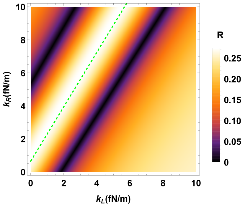
Figure 2: Rectification, R𝑅R, in the kLkRsubscript𝑘𝐿subscript𝑘𝑅k_{L}k_{R} plane for k=1.17×k=1.17\times fN/m, γL=6.75×10²²subscript𝛾𝐿6.75superscript1022\gamma_{L}=6.75\times 10^{-22} kg/s, and γR=4.64γLsubscript𝛾𝑅4.64subscript𝛾𝐿\gamma_{R}=4.64\gamma_{L}.

To measure rectification, we will use the rectification coefficient R𝑅R defined as

R=|JJ~|max(J,J~),𝑅𝐽~𝐽𝐽~𝐽R=\frac{\absolutevalue{J-\tilde{J}}}{\max(J,\tilde{J})}, (35)

that is, the ratio between the difference of heat currents and the largest one. As defined, R=0𝑅0R=0 for no asymmetry of the heat currents and R=1𝑅1R=1 when they are maximally asymmetric.

Table 1: Definition of forward and reversed (exchanged) bath configurations.
forward reversed
Bath Friction γLsubscript𝛾𝐿\gamma_{L}, γRsubscript𝛾𝑅\gamma_{R} γ~L=γRsubscript~𝛾𝐿subscript𝛾𝑅\tilde{\gamma}_{L}=\gamma_{R}, γ~R=γLsubscript~𝛾𝑅subscript𝛾𝐿\tilde{\gamma}_{R}=\gamma_{L}
Bath Temperature TLsubscript𝑇𝐿T_{L}, TRsubscript𝑇𝑅T_{R} T~L=TRsubscript~𝑇𝐿subscript𝑇𝑅\tilde{T}_{L}=T_{R}, T~R=TLsubscript~𝑇𝑅subscript𝑇𝐿\tilde{T}_{R}=T_{L}

VI.1 Parametric exploration

We have explored thoroughly the space formed by the parameters of the model to find asymmetric heat transport, namely, m1,m2,k,kL,kR,γL,γRsubscript𝑚1subscript𝑚2𝑘subscript𝑘𝐿subscript𝑘𝑅subscript𝛾𝐿subscript𝛾𝑅m_{1},m_{2},k,k_{L},k_{R},\gamma_{L},\gamma_{R}. We have fixed the values of some of the parameters to realistic ones while we have varied the rest. We have set the masses to m1=24.305subscript𝑚124.305m_{1}=24.305 a.u. and m2=40.078subscript𝑚240.078m_{2}=40.078 a.u., which correspond to Mg and Ca, whose ions are broadly used in trapped-ion physics. The temperatures are also fixed and, as Eq. (24) shows, rectification does not formally depend on the temperature in this model, unless we set the friction coefficients as a function of temperature using Eq. (34) explicitly.

Figure 2 depicts the values of the rectification after sweeping the kLkRsubscript𝑘𝐿subscript𝑘𝑅k_{L}k_{R} plane for fixed values of k𝑘k, γLsubscript𝛾𝐿\gamma_{L}, and γRsubscript𝛾𝑅\gamma_{R}. A remarkable result from this figure is that parallel lines appear alternating minima and maxima of R𝑅R. With a numerical fitting, we find that the line corresponding to the highest maximum value of R𝑅R is determined by

k+kLm1=k+kRm2.𝑘subscript𝑘𝐿subscript𝑚1𝑘subscript𝑘𝑅subscript𝑚2\frac{k+k_{L}}{m_{1}}=\frac{k+k_{R}}{m_{2}}. (36)

In a trapped-ion context the condition (36) may be imposed by adjusting the distance of the traps for fixed kLsubscript𝑘𝐿k_{L} and kRsubscript𝑘𝑅k_{R}. It is also remarkable that when Eq. (36) is satisfied, the rectification no longer depends on the spring constants of the model. This last result can be found assuming Eq. (36) when calculating the currents with Eq. (24) and R𝑅R with Eq. (35),

R={1a+g1+ag if (a+g)<(1+ag)11+aga+g if (a+g)>(1+ag)0 if (a+g)=(1+ag),𝑅cases1𝑎𝑔1𝑎𝑔 if 𝑎𝑔1𝑎𝑔11𝑎𝑔𝑎𝑔 if 𝑎𝑔1𝑎𝑔0 if 𝑎𝑔1𝑎𝑔R=\begin{cases}1-\frac{a+g}{1+ag}&\text{ if }(a+g)<(1+ag)\\ 1-\frac{1+ag}{a+g}&\text{ if }(a+g)>(1+ag)\\ 0&\text{ if }(a+g)=(1+ag)\,,\end{cases} (37)

where a𝑎a and g𝑔g are the mass and friction coefficients ratios

a𝑎\displaystyle a =m2/m1,absentsubscript𝑚2subscript𝑚1\displaystyle=m_{2}/m_{1},
g𝑔\displaystyle g =γR/γL.absentsubscript𝛾𝑅subscript𝛾𝐿\displaystyle=\gamma_{R}/\gamma_{L}. (38)

The maximal rectification found does not scale with the magnitude of the masses or the friction coefficients, just with their ratios. Besides a high R𝑅R, it is important to have non-vanishing heat currents Simón et al. (2019). Using again Eq. (36) in the expression for the currents (24), the maximum current Jmax=max(|J|,|J~|)subscript𝐽𝐽~𝐽J_{\max}=\max(\big{|}{J}\big{|},\big{|}\tilde{J}\big{|}) is

Jmax={kBgγLk2|TLTR|(a+g)(gγL2(kL+k)+k2m1) if (a+g)<(1+ag)kBgγLk2|TLTR|(1+ag)(gγL2(kL+k)+k2m1) if (a+g)>(1+ag).subscript𝐽casessubscript𝑘𝐵𝑔subscript𝛾𝐿superscript𝑘2subscript𝑇𝐿subscript𝑇𝑅𝑎𝑔𝑔superscriptsubscript𝛾𝐿2subscript𝑘𝐿𝑘superscript𝑘2subscript𝑚1 if 𝑎𝑔1𝑎𝑔subscript𝑘𝐵𝑔subscript𝛾𝐿superscript𝑘2subscript𝑇𝐿subscript𝑇𝑅1𝑎𝑔𝑔superscriptsubscript𝛾𝐿2subscript𝑘𝐿𝑘superscript𝑘2subscript𝑚1 if 𝑎𝑔1𝑎𝑔\displaystyle J_{\max}=\begin{cases}\frac{k_{B}g\gamma_{L}k^{2}\absolutevalue{T_{L}-T_{R}}}{(a+g)(g\gamma_{L}^{2}(k_{L}+k)+k^{2}m_{1})}&\text{ if }(a+g)<(1+ag)\\ \frac{k_{B}g\gamma_{L}k^{2}\absolutevalue{T_{L}-T_{R}}}{(1+ag)(g\gamma_{L}^{2}(k_{L}+k)+k^{2}m_{1})}&\text{ if }(a+g)>(1+ag)\,.\end{cases} (39)

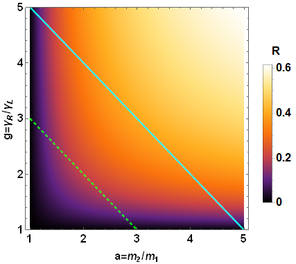
Now we analyze how the parameters a𝑎a and g𝑔g affect the maximum current Jmaxsubscript𝐽𝑚𝑎𝑥J_{max} in (39). To do this, we can divide the ag𝑎𝑔ag plane in four quadrants by the axes a=1𝑎1a=1 and g=1𝑔1g=1 (in those axes R=0𝑅0R=0). In Eq. (39) the parameter a𝑎a appears only in the denominator, thus for a higher a𝑎a, a smaller current is found. The quadrants with a<1𝑎1a<1 will be better for achieving large currents. However, g𝑔g appears both in the numerator and denominator so there is no obvious advantageous quadrant for this parameter.

Equation (37) is symmetric upon the transformations a1/a𝑎1𝑎a\leftrightarrow 1/a and g1/g𝑔1𝑔g\leftrightarrow 1/g. Using a logarithmic scale for a𝑎a and g𝑔g, the resulting R𝑅R map will be symmetric with respect to the a=1𝑎1a=1 and g=1𝑔1g=1 axes. We can limit ourselves to analyze the quadrant a>1𝑎1a>1, g>1𝑔1g>1, as the results in other quadrants will be equivalent upon transformations a1/a𝑎1𝑎a\leftrightarrow 1/a and g1/g𝑔1𝑔g\leftrightarrow 1/g.

Refer to caption
Figure 3: Rectification factor, R𝑅R, given by Eq. (37).

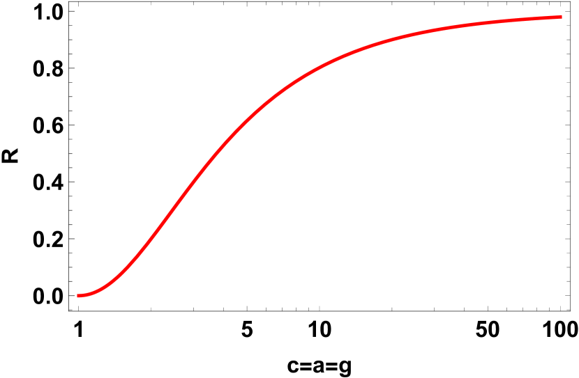
Fig. 3 shows the rectification given by Eq. (37) in terms of a𝑎a and g𝑔g. Along any diagonal line (parallel to the solid cyan or the dashed green lines), the maximum value is at the center, that is, when a=g𝑎𝑔a=g. However, if we fix a𝑎a, increasing g𝑔g always increases R𝑅R. Although we could increase g𝑔g arbitrarily to get more rectification this is not a realistic option in a trapped-ion set-up. Since g𝑔g is defined as the ratio between the friction coefficients, increasing it means making either γLsubscript𝛾𝐿\gamma_{L} go to 0 or γRsubscript𝛾𝑅\gamma_{R} to infinity. Making γLsubscript𝛾𝐿\gamma_{L} go to 0 decouples one of the ions from the bath, so the heat current tends to vanish in any direction. Also, increasing γRsubscript𝛾𝑅\gamma_{R} arbitrarily is impossible since the Doppler cooling friction coefficient as a function of the laser detuning (Eq. (34)) is bounded. Although Eq. (34) suggests that boosting the laser intensity can also increase the friction coefficient, this is not an option since Eq. (34) is just an approximation for low laser intensities. When going to higher intensities, the emission/absorption of photons by the ion is saturated and the friction coefficient reaches a finite value proportional to the width ΓΓ\Gamma of the excited state Metcalf and van der Straten (2003). As a compromise between feasibility and high R𝑅R, we set the ratio between the friction coefficients g𝑔g to be equal to the mass ratio a𝑎a. As shown in Fig. 3, along the solid-cyan and dashed-green diagonal lines the maximum R𝑅R is achieved for a=g𝑎𝑔a=g. Fig. 4 shows the rectification in Eq. (37) for the line a=g𝑎𝑔a=g. When both parameters are large enough, the rectification goes to 1.

VI.2 Spectral match/mismatch approach to rectification
Refer to caption
Figure 4: Rectification for different values of c=m2/m1=γR/γL𝑐subscript𝑚2subscript𝑚1subscript𝛾𝑅subscript𝛾𝐿c=m_{2}/m_{1}=\gamma_{R}/\gamma_{L} when the maximum condition in the kLkRsubscript𝑘𝐿subscript𝑘𝑅k_{L}k_{R} plane is satisfied (Eq. (36)).

The match/mismatch between the power spectra of the particles controls the heat currents in the system Terraneo et al. (2002); Li et al. (2004). A good match between the power spectra of the two ions in a large range of frequencies yields a higher heat current through the system while the mismatch reduces the heat current. If there is a good match between the spectra of the ions (i.e., their peaks overlap in a broad range of frequencies) for a certain baths configuration, and mismatch when the baths exchange, the system will present heat rectification.

We have studied the phonon spectra of our model for several sets of parameters exhibiting no rectification or strong rectification. The phonon spectra of the ions is calculated through the spectral density matrix. For a real-valued stochastic process x(t)𝑥𝑡\overrightarrow{x}(t), its spectral density matrix is defined as Särkkä and Solin (2019)

𝕊x(ω)X(ω)X𝖳(ω),subscript𝕊𝑥𝜔expectation-value𝑋𝜔superscript𝑋𝖳𝜔\mathbb{S}_{\overrightarrow{x}}(\omega)\equiv\expectationvalue{\overrightarrow{X}(\omega)\overrightarrow{X}^{\mathsf{T}}(-\omega)}, (40)

with X(ω)𝑋𝜔\overrightarrow{X}(\omega) being the Fourier transform of x(t)𝑥𝑡\overrightarrow{x}(t) (we are using the convention of multiplying by a factor of 111 and 12π12𝜋\frac{1}{2\pi} for the transform and its inverse operation). A justification of the use of the spectral density matrix to understand heat transport arises from the Wiener-Khinchin theorem Särkkä and Solin (2019), which says that the correlation matrix of a stationary stochastic process in the steady state is the inverse Fourier transform of its spectral density matrix r(t)r𝖳(t+τ)=1[𝕊r(ω)](τ)expectation-value𝑟𝑡superscript𝑟𝖳𝑡𝜏superscript1delimited-[]subscript𝕊𝑟𝜔𝜏\expectationvalue{\overrightarrow{r}(t)\overrightarrow{r}^{\mathsf{T}}(t+\tau)}=\mathcal{F}^{-1}[\mathbb{S}_{\overrightarrow{r}}(\omega)](\tau). This result allows us to write down the covariance matrix in the steady state through the spectral density as

s.s.=12π𝑑ω𝕊r(ω).superscriptformulae-sequence𝑠𝑠12𝜋superscriptsubscriptdifferential-d𝜔subscript𝕊𝑟𝜔\mathbb{C}^{s.s.}=\frac{1}{2\pi}\int_{-\infty}^{\infty}d\omega\;\mathbb{S}_{\overrightarrow{r}}(\omega). (41)

Eq. (41) directly connects the spectral density matrix to the steady-state temperature and, therefore, to the heat currents (in Section III we saw that T1s.s.=m1C3,3s.s./kBsuperscriptsubscript𝑇1formulae-sequence𝑠𝑠subscript𝑚1superscriptsubscript𝐶33formulae-sequence𝑠𝑠subscript𝑘𝐵T_{1}^{s.s.}={m_{1}C_{3,3}^{s.s.}}/{k_{B}} and T2s.s.=m2C4,4s.s./kBsuperscriptsubscript𝑇2formulae-sequence𝑠𝑠subscript𝑚2superscriptsubscript𝐶44formulae-sequence𝑠𝑠subscript𝑘𝐵T_{2}^{s.s.}={m_{2}C_{4,4}^{s.s.}}/{k_{B}}).

Refer to caption
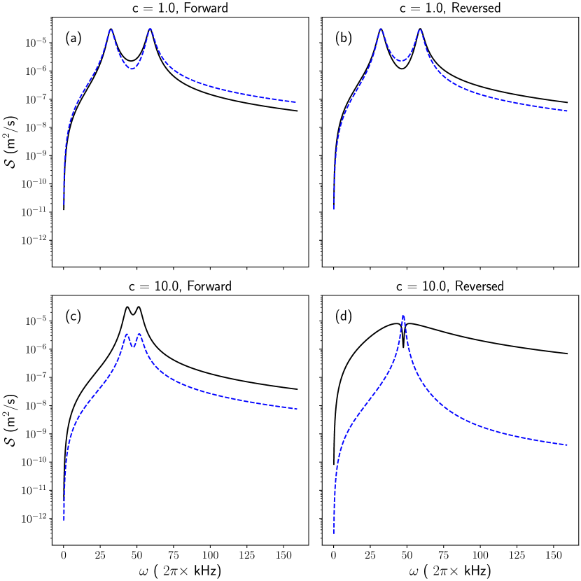
Figure 5: Spectral densities of the velocities of the ions (r3subscript𝑟3r_{3} and r4subscript𝑟4r_{4}) corresponding to different values of c𝑐c in Fig. 4: (a), (b) for c=1𝑐1c=1 and (c), (d) for c=10𝑐10c=10. Solid, black lines correspond to the left ion velocity spectral density 𝕊3,3(ω)subscript𝕊33𝜔\mathbb{S}_{3,3}(\omega) and dashed, blue lines correspond to the right ion velocity spectral density 𝕊4,4(ω)subscript𝕊44𝜔\mathbb{S}_{4,4}(\omega). (a) and (b) correspond to R=0𝑅0R=0: the overlap between the phonon bands is the same in the forward and reversed configurations. (c) and (d) correspond to R0.8𝑅0.8R\approx 0.8: in the forward configuration (c) the phonons match better than in the reversed configuration (d).

For the vector process r(t)𝑟𝑡\overrightarrow{r}(t) describing the evolution of our system we have R(ω)=(iω𝔸)1𝕃Ξ(ω)𝑅𝜔superscript𝑖𝜔𝔸1𝕃Ξ𝜔\overrightarrow{R}(\omega)=\left(i\omega-\mathbb{A}\right)^{-1}\mathbb{L}\overrightarrow{\Xi}(\omega) with Ξ(ω)Ξ𝜔\overrightarrow{\Xi}(\omega) being the Fourier transform of the white noise ξ(t)𝜉𝑡\overrightarrow{\xi}(t). Note that Ξ(ω)Ξ𝜔\overrightarrow{\Xi}(\omega) does not strictly exist, because it is not square-integrable, however its spectral density is 𝕊ξ(ω)=2𝔻subscript𝕊𝜉𝜔2𝔻\mathbb{S}_{\overrightarrow{\xi}}(\omega)=2\mathbb{D} Särkkä and Solin (2019), which is flat as expected for a white noise. Therefore, the spectral density matrix of the system is

𝕊r=2(𝔸iω)1𝕃𝔻𝕃𝖳(𝔸+iω)𝖳.subscript𝕊𝑟2superscript𝔸𝑖𝜔1𝕃𝔻superscript𝕃𝖳superscript𝔸𝑖𝜔𝖳\mathbb{S}_{\overrightarrow{r}}=2\left(\mathbb{A}-i\omega\right)^{-1}\mathbb{L}\mathbb{D}\mathbb{L}^{\mathsf{T}}\left(\mathbb{A}+i\omega\right)^{-\mathsf{T}}. (42)

As we can see in Eq. (42), the imaginary part of the eigenvalues of the dynamical matrix 𝔸𝔸\mathbb{A} correspond to the peaks in the spectrum whereas the real part dictates their width. The spectral density matrix of our model is

𝕊r(ω)=2kBγLTL𝕊L(iω)+γLTR𝕊R(iω)(m1m2)2P𝔸(iω)P𝔸(iω),subscript𝕊𝑟𝜔2subscript𝑘𝐵subscript𝛾𝐿subscript𝑇𝐿subscript𝕊𝐿𝑖𝜔subscript𝛾𝐿subscript𝑇𝑅subscript𝕊𝑅𝑖𝜔superscriptsubscript𝑚1subscript𝑚22subscript𝑃𝔸𝑖𝜔subscript𝑃𝔸𝑖𝜔\mathbb{S}_{\overrightarrow{r}}(\omega)=2k_{B}\frac{\gamma_{L}T_{L}\mathbb{S}_{L}(i\omega)+\gamma_{L}T_{R}\mathbb{S}_{R}(i\omega)}{(m_{1}m_{2})^{2}P_{\mathbb{A}}(i\omega)P_{\mathbb{A}}(-i\omega)}, (43)

where P𝔸(λ)subscript𝑃𝔸𝜆P_{\mathbb{A}}(\lambda) is the characteristic polynomial of the dynamical matrix 𝔸𝔸\mathbb{A} and 𝕊L(ω)subscript𝕊𝐿𝜔\mathbb{S}_{L}(\omega), 𝕊R(ω)subscript𝕊𝑅𝜔\mathbb{S}_{R}(\omega) are the matrix polynomials in the angular frequency ω𝜔\omega whose coefficients are defined in Appendix B. Equation (44) gives the full expressions of the spectral densities for the velocities, 𝕊3,3(ω)=R3(ω)R3(ω)subscript𝕊33𝜔expectation-valuesubscript𝑅3𝜔subscript𝑅3𝜔\mathbb{S}_{3,3}(\omega)=\expectationvalue{R_{3}(\omega)R_{3}(-\omega)} for the left ion, and 𝕊4,4(ω)=R4(ω)R4(ω)subscript𝕊44𝜔expectation-valuesubscript𝑅4𝜔subscript𝑅4𝜔\mathbb{S}_{4,4}(\omega)=\expectationvalue{R_{4}(\omega)R_{4}(-\omega)} for the right ion, since they are the elements related to the calculation of the heat current using Eq. (41),

𝕊3,3(ω)subscript𝕊33𝜔\displaystyle\mathbb{S}_{3,3}(\omega) =2kBγRk2TRω2+γLTL[ω4(γR22km22kRm2)+ω2(k+kR)2+m22ω6](m1m2)2P𝔸(iω)P𝔸(iω),absent2subscript𝑘𝐵subscript𝛾𝑅superscript𝑘2subscript𝑇𝑅superscript𝜔2subscript𝛾𝐿subscript𝑇𝐿delimited-[]superscript𝜔4superscriptsubscript𝛾𝑅22𝑘subscript𝑚22subscript𝑘𝑅subscript𝑚2superscript𝜔2superscript𝑘subscript𝑘𝑅2superscriptsubscript𝑚22superscript𝜔6superscriptsubscript𝑚1subscript𝑚22subscript𝑃𝔸𝑖𝜔subscript𝑃𝔸𝑖𝜔\displaystyle=2k_{B}\frac{\gamma_{R}k^{2}T_{R}\omega^{2}+\gamma_{L}T_{L}\left[\omega^{4}\left(\gamma_{R}^{2}-2km_{2}-2k_{R}m_{2}\right)+\omega^{2}(k+k_{R})^{2}+m_{2}^{2}\omega^{6}\right]}{(m_{1}m_{2})^{2}P_{\mathbb{A}}(i\omega)P_{\mathbb{A}}(-i\omega)},
𝕊4,4(ω)subscript𝕊44𝜔\displaystyle\mathbb{S}_{4,4}(\omega) =2kBγLk2TLω2+γRTR[ω4(γL22km12kLm1)+ω2(k+kL)2+m12ω6](m1m2)2P𝔸(iω)P𝔸(iω).absent2subscript𝑘𝐵subscript𝛾𝐿superscript𝑘2subscript𝑇𝐿superscript𝜔2subscript𝛾𝑅subscript𝑇𝑅delimited-[]superscript𝜔4superscriptsubscript𝛾𝐿22𝑘subscript𝑚12subscript𝑘𝐿subscript𝑚1superscript𝜔2superscript𝑘subscript𝑘𝐿2superscriptsubscript𝑚12superscript𝜔6superscriptsubscript𝑚1subscript𝑚22subscript𝑃𝔸𝑖𝜔subscript𝑃𝔸𝑖𝜔\displaystyle=2k_{B}\frac{\gamma_{L}k^{2}T_{L}\omega^{2}+\gamma_{R}T_{R}\left[\omega^{4}\left(\gamma_{L}^{2}-2km_{1}-2k_{L}m_{1}\right)+\omega^{2}(k+k_{L})^{2}+m_{1}^{2}\omega^{6}\right]}{(m_{1}m_{2})^{2}P_{\mathbb{A}}(i\omega)P_{\mathbb{A}}(-i\omega)}. (44)

Figure 5 depicts a series of plots of the spectra given by Eq. (44) that correspond to two points in Fig. 4. For c=1𝑐1c=1 (Fig. 5(a) and (b)) there is no rectification, since the spectra match in the forward (a) and reversed (b) configurations. However, for c=10𝑐10c=10 ((Fig. 5(c) and (d))) the picture is very different: there is a good match between the spectra in the forward configuration whereas in the reversed configuration the spectra are less correlated, giving as a result higher rectification (R0.8𝑅0.8R\approx 0.8). Figure 5 only shows the elements (3,3) and (4,4) in the diagonal of 𝕊𝕊\mathbb{S} but the remaining elements, including off-diagonal ones, exhibit a similar behavior.

VII Conclusions

We have studied heat rectification in a model composed of two coupled harmonic oscillators connected to baths. This simple model allows analytical treatment but still has enough complexity to examine different ingredients that can produce rectification. Our results demonstrate in a simple but realistic system that harmonic systems can rectificate heat current if they have features which depend on the temperature Pereira (2017). We implement this notion of temperature-dependent features by defining the baths exchange operation as an exchange of both temperatures and coupling parameters of the baths to the system. This kind of temperature-dependent features happens naturally in laser-cooled trapped ion set-ups.

We have also studied the phonon spectra of the system, comparing the match/mismatch of the phonon bands, to reach the conclusion that the band match/mismatch description for heat rectification is also valid for systems which are harmonic, as long as there are temperature-dependent features. We hope this article sheds more light into the topic of heat rectification and that encourages more research regarding its physical implementation on chains of trapped ions.

VIII acknowledgements

We thank Daniel Alonso for fruitful discussions and comments. This work was supported by the Basque Country Government (Grant No. IT986-16), by Grants PGC2018-101355-B-I00 (MCIU/AEI/FEDER,UE) and FIS2016-80681P, and by the Spanish MICINN and European Union (FEDER) (Grant No. FIS2017-82855-P). M.A.S. acknowledges support by the Basque Government predoctoral program (Grant No. PRE-2019-2-0234).

References

Appendix A Full set of steady-state equations for the components of s.ssuperscriptformulae-sequence𝑠𝑠\mathbb{C}^{s.s}

Here we present the full set of equations for the covariance matrix elements in the steady state,

2kp2q1s.s.m1m2+2γLp12s.s.m13=2DLm12,2kp2q1s.s.m22+2γRp22s.s.m23=2DRm22,(kL+k)q1q2s.s.m1+kq22s.s.m1+γLp2q1s.s.m1m2+p1p2s.s.m1m2=0,(kL+k)p2q1s.s.m1m2(kR+k)p2q1s.s.m22+γLp1p2s.s.m12m2+γRp1p2s.s.m1m22=0,(kL+k)q12s.s.m1+kq1q2s.s.m1+p12s.s.m12=0,(kR+k)q22s.s.m2+kq1q2s.s.m2+p22s.s.m22=0,(kR+k)q1q2s.s.m2+kq12s.s.m2γRp2q1s.s.m22+p1p2s.s.m1m2=0formulae-sequence2𝑘superscriptexpectation-valuesubscript𝑝2subscript𝑞1formulae-sequence𝑠𝑠subscript𝑚1subscript𝑚22subscript𝛾𝐿superscriptexpectation-valuesuperscriptsubscript𝑝12formulae-sequence𝑠𝑠superscriptsubscript𝑚132subscript𝐷𝐿superscriptsubscript𝑚12formulae-sequence2𝑘superscriptexpectation-valuesubscript𝑝2subscript𝑞1formulae-sequence𝑠𝑠superscriptsubscript𝑚222subscript𝛾𝑅superscriptexpectation-valuesuperscriptsubscript𝑝22formulae-sequence𝑠𝑠superscriptsubscript𝑚232subscript𝐷𝑅superscriptsubscript𝑚22formulae-sequencesubscript𝑘𝐿𝑘superscriptexpectation-valuesubscript𝑞1subscript𝑞2formulae-sequence𝑠𝑠subscript𝑚1𝑘superscriptexpectation-valuesuperscriptsubscript𝑞22formulae-sequence𝑠𝑠subscript𝑚1subscript𝛾𝐿superscriptexpectation-valuesubscript𝑝2subscript𝑞1formulae-sequence𝑠𝑠subscript𝑚1subscript𝑚2superscriptexpectation-valuesubscript𝑝1subscript𝑝2formulae-sequence𝑠𝑠subscript𝑚1subscript𝑚20formulae-sequencesubscript𝑘𝐿𝑘superscriptexpectation-valuesubscript𝑝2subscript𝑞1formulae-sequence𝑠𝑠subscript𝑚1subscript𝑚2subscript𝑘𝑅𝑘superscriptexpectation-valuesubscript𝑝2subscript𝑞1formulae-sequence𝑠𝑠superscriptsubscript𝑚22subscript𝛾𝐿superscriptexpectation-valuesubscript𝑝1subscript𝑝2formulae-sequence𝑠𝑠superscriptsubscript𝑚12subscript𝑚2subscript𝛾𝑅superscriptexpectation-valuesubscript𝑝1subscript𝑝2formulae-sequence𝑠𝑠subscript𝑚1superscriptsubscript𝑚220formulae-sequencesubscript𝑘𝐿𝑘superscriptexpectation-valuesuperscriptsubscript𝑞12formulae-sequence𝑠𝑠subscript𝑚1𝑘superscriptexpectation-valuesubscript𝑞1subscript𝑞2formulae-sequence𝑠𝑠subscript𝑚1superscriptexpectation-valuesuperscriptsubscript𝑝12formulae-sequence𝑠𝑠superscriptsubscript𝑚120formulae-sequencesubscript𝑘𝑅𝑘superscriptexpectation-valuesuperscriptsubscript𝑞22formulae-sequence𝑠𝑠subscript𝑚2𝑘superscriptexpectation-valuesubscript𝑞1subscript𝑞2formulae-sequence𝑠𝑠subscript𝑚2superscriptexpectation-valuesuperscriptsubscript𝑝22formulae-sequence𝑠𝑠superscriptsubscript𝑚220subscript𝑘𝑅𝑘superscriptexpectation-valuesubscript𝑞1subscript𝑞2formulae-sequence𝑠𝑠subscript𝑚2𝑘superscriptexpectation-valuesuperscriptsubscript𝑞12formulae-sequence𝑠𝑠subscript𝑚2subscript𝛾𝑅superscriptexpectation-valuesubscript𝑝2subscript𝑞1formulae-sequence𝑠𝑠superscriptsubscript𝑚22superscriptexpectation-valuesubscript𝑝1subscript𝑝2formulae-sequence𝑠𝑠subscript𝑚1subscript𝑚20\begin{split}\frac{2k\expectationvalue{p_{2}q_{1}}^{s.s.}}{m_{1}m_{2}}+\frac{2\gamma_{L}\expectationvalue{p_{1}^{2}}^{s.s.}}{m_{1}^{3}}&=\frac{2D_{L}}{m_{1}^{2}},\\ -\frac{2k\expectationvalue{p_{2}q_{1}}^{s.s.}}{m_{2}^{2}}+\frac{2\gamma_{R}\expectationvalue{p_{2}^{2}}^{s.s.}}{m_{2}^{3}}&=\frac{2D_{R}}{m_{2}^{2}},\\ -\frac{\left(k_{L}+k\right)\expectationvalue{q_{1}q_{2}}^{s.s.}}{m_{1}}+\frac{k\expectationvalue{q_{2}^{2}}^{s.s.}}{m_{1}}+\frac{\gamma_{L}\expectationvalue{p_{2}q_{1}}^{s.s.}}{m_{1}m_{2}}+\frac{\expectationvalue{p_{1}p_{2}}^{s.s.}}{m_{1}m_{2}}&=0,\\ \frac{\left(k_{L}+k\right)\expectationvalue{p_{2}q_{1}}^{s.s.}}{m_{1}m_{2}}-\frac{\left(k_{R}+k\right)\expectationvalue{p_{2}q_{1}}^{s.s.}}{m_{2}^{2}}+\frac{\gamma_{L}\expectationvalue{p_{1}p_{2}}^{s.s.}}{m_{1}^{2}m_{2}}+\frac{\gamma_{R}\expectationvalue{p_{1}p_{2}}^{s.s.}}{m_{1}m_{2}^{2}}&=0,\\ -\frac{\left(k_{L}+k\right)\expectationvalue{q_{1}^{2}}^{s.s.}}{m_{1}}+\frac{k\expectationvalue{q_{1}q_{2}}^{s.s.}}{m_{1}}+\frac{\expectationvalue{p_{1}^{2}}^{s.s.}}{m_{1}^{2}}&=0,\\ -\frac{\left(k_{R}+k\right)\expectationvalue{q_{2}^{2}}^{s.s.}}{m_{2}}+\frac{k\expectationvalue{q_{1}q_{2}}^{s.s.}}{m_{2}}+\frac{\expectationvalue{p_{2}^{2}}^{s.s.}}{m_{2}^{2}}&=0,\\ -\frac{\left(k_{R}+k\right)\expectationvalue{q_{1}q_{2}}^{s.s.}}{m_{2}}+\frac{k\expectationvalue{q_{1}^{2}}^{s.s.}}{m_{2}}-\frac{\gamma_{R}\expectationvalue{p_{2}q_{1}}^{s.s.}}{m_{2}^{2}}+\frac{\expectationvalue{p_{1}p_{2}}^{s.s.}}{m_{1}m_{2}}&=0\end{split} (45)

Appendix B Complete expressions for the Spectral Density Matrix

In Section VI we used the characteristic polynomial P𝔸(λ)subscript𝑃𝔸𝜆P_{\mathbb{A}}(\lambda) of the dynamical matrix 𝔸𝔸\mathbb{A} for the calculation of the spectral density matrix. P𝔸(λ)subscript𝑃𝔸𝜆P_{\mathbb{A}}(\lambda) is defined as

det(𝔸λ)=λ4+λ3(γLm1+γRm2)+λ2(γLγR+m2(k+kL)+m1(k+kR))m1m2+λ(γR(k+kL)+γL(k+kR))m1m2+k(kL+kR)+kLkRm1m2.𝔸𝜆superscript𝜆4superscript𝜆3subscript𝛾𝐿subscript𝑚1subscript𝛾𝑅subscript𝑚2superscript𝜆2subscript𝛾𝐿subscript𝛾𝑅subscript𝑚2𝑘subscript𝑘𝐿subscript𝑚1𝑘subscript𝑘𝑅subscript𝑚1subscript𝑚2𝜆subscript𝛾𝑅𝑘subscript𝑘𝐿subscript𝛾𝐿𝑘subscript𝑘𝑅subscript𝑚1subscript𝑚2𝑘subscript𝑘𝐿subscript𝑘𝑅subscript𝑘𝐿subscript𝑘𝑅subscript𝑚1subscript𝑚2\begin{split}\det(\mathbb{A}-\lambda)&=\lambda^{4}\\ &+\lambda^{3}\left(\frac{\gamma_{L}}{m_{1}}+\frac{\gamma_{R}}{m_{2}}\right)\\ &+\lambda^{2}\frac{(\gamma_{L}\gamma_{R}+m_{2}(k+k_{L})+m_{1}(k+k_{R}))}{m_{1}m_{2}}\\ &+\lambda\frac{(\gamma_{R}(k+k_{L})+\gamma_{L}(k+k_{R}))}{m_{1}m_{2}}\\ &+\frac{k(k_{L}+k_{R})+k_{L}k_{R}}{m_{1}m_{2}}.\end{split} (46)

We also used the polynomials 𝕊L(λ)subscript𝕊𝐿𝜆\mathbb{S}_{L}(\lambda) and 𝕊R(λ)subscript𝕊𝑅𝜆\mathbb{S}_{R}(\lambda), which are defined as 𝕊L(λ)=n=06λn𝕤L,nsubscript𝕊𝐿𝜆superscriptsubscript𝑛06superscript𝜆𝑛subscript𝕤𝐿𝑛\mathbb{S}_{L}(\lambda)=\sum\limits_{n=0}^{6}\lambda^{n}\mathbb{s}_{L,n} and 𝕊R(λ)=n=06λn𝕤R,nsubscript𝕊𝑅𝜆superscriptsubscript𝑛06superscript𝜆𝑛subscript𝕤𝑅𝑛\mathbb{S}_{R}(\lambda)=\sum\limits_{n=0}^{6}\lambda^{n}\mathbb{s}_{R,n}. There are 14 different polynomial coefficients, which are 4×4444\times 4 matrices, which makes very cumbersome to include them in the main text. This is the full list of coefficients,

𝕤L,0subscript𝕤𝐿0\displaystyle\mathbb{s}_{L,0} =((k+kR)2k(k+kR)00k(k+kR)k20000000000),absentsuperscript𝑘subscript𝑘𝑅2𝑘𝑘subscript𝑘𝑅00𝑘𝑘subscript𝑘𝑅superscript𝑘20000000000\displaystyle=\left(\begin{array}[]{cccc}(k+k_{R})^{2}&k(k+k_{R})&0&0\\ k(k+k_{R})&k^{2}&0&0\\ 0&0&0&0\\ 0&0&0&0\end{array}\right), 𝕤R,0subscript𝕤𝑅0\displaystyle\mathbb{s}_{R,0} =(k2k(k+kL)00k(k+kL)(k+kL)20000000000),absentsuperscript𝑘2𝑘𝑘subscript𝑘𝐿00𝑘𝑘subscript𝑘𝐿superscript𝑘subscript𝑘𝐿20000000000\displaystyle=\left(\begin{array}[]{cccc}k^{2}&k(k+k_{L})&0&0\\ k(k+k_{L})&(k+k_{L})^{2}&0&0\\ 0&0&0&0\\ 0&0&0&0\end{array}\right), (47)
𝕤L,1subscript𝕤𝐿1\displaystyle\mathbb{s}_{L,1} =(0kγR(k+kR)2k(k+kR)kγR0k(k+kR)k2(k+kR)2k(k+kR)00k(k+kR)k200),absent0𝑘subscript𝛾𝑅superscript𝑘subscript𝑘𝑅2𝑘𝑘subscript𝑘𝑅𝑘subscript𝛾𝑅0𝑘𝑘subscript𝑘𝑅superscript𝑘2superscript𝑘subscript𝑘𝑅2𝑘𝑘subscript𝑘𝑅00𝑘𝑘subscript𝑘𝑅superscript𝑘200\displaystyle=\left(\begin{array}[]{cccc}0&k\gamma_{R}&-(k+k_{R})^{2}&-k(k+k_{R})\\ -k\gamma_{R}&0&-k(k+k_{R})&-k^{2}\\ (k+k_{R})^{2}&k(k+k_{R})&0&0\\ k(k+k_{R})&k^{2}&0&0\end{array}\right), 𝕤R,1subscript𝕤𝑅1\displaystyle\mathbb{s}_{R,1} =(0kγLk2k(k+kL)kγL0k(k+kL)(k+kL)2k2k(k+kL)00k(k+kL)(k+kL)200),absent0𝑘subscript𝛾𝐿superscript𝑘2𝑘𝑘subscript𝑘𝐿𝑘subscript𝛾𝐿0𝑘𝑘subscript𝑘𝐿superscript𝑘subscript𝑘𝐿2superscript𝑘2𝑘𝑘subscript𝑘𝐿00𝑘𝑘subscript𝑘𝐿superscript𝑘subscript𝑘𝐿200\displaystyle=\left(\begin{array}[]{cccc}0&-k\gamma_{L}&-k^{2}&-k(k+k_{L})\\ k\gamma_{L}&0&-k(k+k_{L})&-(k+k_{L})^{2}\\ k^{2}&k(k+k_{L})&0&0\\ k(k+k_{L})&(k+k_{L})^{2}&0&0\end{array}\right),
𝕤L,2subscript𝕤𝐿2\displaystyle\mathbb{s}_{L,2} =(2(k+kR)m2γR2km20kγRkm20kγR00kγR(k+kR)2k(k+kR)kγR0k(k+kR)k2),absent2𝑘subscript𝑘𝑅subscript𝑚2superscriptsubscript𝛾𝑅2𝑘subscript𝑚20𝑘subscript𝛾𝑅𝑘subscript𝑚20𝑘subscript𝛾𝑅00𝑘subscript𝛾𝑅superscript𝑘subscript𝑘𝑅2𝑘𝑘subscript𝑘𝑅𝑘subscript𝛾𝑅0𝑘𝑘subscript𝑘𝑅superscript𝑘2\displaystyle=\left(\begin{array}[]{cccc}2(k+k_{R})m_{2}-\gamma_{R}^{2}&km_{2}&0&-k\gamma_{R}\\ km_{2}&0&k\gamma_{R}&0\\ 0&k\gamma_{R}&-(k+k_{R})^{2}&-k(k+k_{R})\\ -k\gamma_{R}&0&-k(k+k_{R})&-k^{2}\end{array}\right), 𝕤R,2subscript𝕤𝑅2\displaystyle\mathbb{s}_{R,2} =(0km10kγLkm12(k+kL)m1γL2kγL00kγLk2k(k+kL)kγL0k(k+kL)(k+kL)2),absent0𝑘subscript𝑚10𝑘subscript𝛾𝐿𝑘subscript𝑚12𝑘subscript𝑘𝐿subscript𝑚1superscriptsubscript𝛾𝐿2𝑘subscript𝛾𝐿00𝑘subscript𝛾𝐿superscript𝑘2𝑘𝑘subscript𝑘𝐿𝑘subscript𝛾𝐿0𝑘𝑘subscript𝑘𝐿superscript𝑘subscript𝑘𝐿2\displaystyle=\left(\begin{array}[]{cccc}0&km_{1}&0&k\gamma_{L}\\ km_{1}&2(k+k_{L})m_{1}-\gamma_{L}^{2}&-k\gamma_{L}&0\\ 0&-k\gamma_{L}&-k^{2}&-k(k+k_{L})\\ k\gamma_{L}&0&-k(k+k_{L})&-(k+k_{L})^{2}\end{array}\right),
𝕤L,3subscript𝕤𝐿3\displaystyle\mathbb{s}_{L,3} =(00γR22(k+kR)m2km200km202(k+kR)m2γR2km20kγRkm20kγR0),absent00superscriptsubscript𝛾𝑅22𝑘subscript𝑘𝑅subscript𝑚2𝑘subscript𝑚200𝑘subscript𝑚202𝑘subscript𝑘𝑅subscript𝑚2superscriptsubscript𝛾𝑅2𝑘subscript𝑚20𝑘subscript𝛾𝑅𝑘subscript𝑚20𝑘subscript𝛾𝑅0\displaystyle=\left(\begin{array}[]{cccc}0&0&\gamma_{R}^{2}-2(k+k_{R})m_{2}&-km_{2}\\ 0&0&-km_{2}&0\\ 2(k+k_{R})m_{2}-\gamma_{R}^{2}&km_{2}&0&-k\gamma_{R}\\ km_{2}&0&k\gamma_{R}&0\end{array}\right), 𝕤R,3subscript𝕤𝑅3\displaystyle\mathbb{s}_{R,3} =(000km100km1γL22(k+kL)m10km10kγLkm12(k+kL)m1γL2kγL0),absent000𝑘subscript𝑚100𝑘subscript𝑚1superscriptsubscript𝛾𝐿22𝑘subscript𝑘𝐿subscript𝑚10𝑘subscript𝑚10𝑘subscript𝛾𝐿𝑘subscript𝑚12𝑘subscript𝑘𝐿subscript𝑚1superscriptsubscript𝛾𝐿2𝑘subscript𝛾𝐿0\displaystyle=\left(\begin{array}[]{cccc}0&0&0&-km_{1}\\ 0&0&-km_{1}&\gamma_{L}^{2}-2(k+k_{L})m_{1}\\ 0&km_{1}&0&k\gamma_{L}\\ km_{1}&2(k+k_{L})m_{1}-\gamma_{L}^{2}&-k\gamma_{L}&0\end{array}\right),
𝕤L,4subscript𝕤𝐿4\displaystyle\mathbb{s}_{L,4} =(m22000000000γR22(k+kR)m2km200km20),absentsuperscriptsubscript𝑚22000000000superscriptsubscript𝛾𝑅22𝑘subscript𝑘𝑅subscript𝑚2𝑘subscript𝑚200𝑘subscript𝑚20\displaystyle=\left(\begin{array}[]{cccc}m_{2}^{2}&0&0&0\\ 0&0&0&0\\ 0&0&\gamma_{R}^{2}-2(k+k_{R})m_{2}&-km_{2}\\ 0&0&-km_{2}&0\end{array}\right), 𝕤R,4subscript𝕤𝑅4\displaystyle\mathbb{s}_{R,4} =(00000m1200000km100km1γL22(k+kL)m1),absent00000superscriptsubscript𝑚1200000𝑘subscript𝑚100𝑘subscript𝑚1superscriptsubscript𝛾𝐿22𝑘subscript𝑘𝐿subscript𝑚1\displaystyle=\left(\begin{array}[]{cccc}0&0&0&0\\ 0&m_{1}^{2}&0&0\\ 0&0&0&-km_{1}\\ 0&0&-km_{1}&\gamma_{L}^{2}-2(k+k_{L})m_{1}\end{array}\right),
𝕤L,5subscript𝕤𝐿5\displaystyle\mathbb{s}_{L,5} =(00m2200000m220000000),absent00superscriptsubscript𝑚2200000superscriptsubscript𝑚220000000\displaystyle=\left(\begin{array}[]{cccc}0&0&-m_{2}^{2}&0\\ 0&0&0&0\\ m_{2}^{2}&0&0&0\\ 0&0&0&0\end{array}\right), 𝕤R,5subscript𝕤𝑅5\displaystyle\mathbb{s}_{R,5} =(0000000m1200000m1200),absent0000000superscriptsubscript𝑚1200000superscriptsubscript𝑚1200\displaystyle=\left(\begin{array}[]{cccc}0&0&0&0\\ 0&0&0&-m_{1}^{2}\\ 0&0&0&0\\ 0&m_{1}^{2}&0&0\end{array}\right),
𝕤L,6subscript𝕤𝐿6\displaystyle\mathbb{s}_{L,6} =(0000000000m2200000),absent0000000000superscriptsubscript𝑚2200000\displaystyle=\left(\begin{array}[]{cccc}0&0&0&0\\ 0&0&0&0\\ 0&0&-m_{2}^{2}&0\\ 0&0&0&0\end{array}\right), 𝕤R,6subscript𝕤𝑅6\displaystyle\mathbb{s}_{R,6} =(000000000000000m12).absent000000000000000superscriptsubscript𝑚12\displaystyle=\left(\begin{array}[]{cccc}0&0&0&0\\ 0&0&0&0\\ 0&0&0&0\\ 0&0&0&-m_{1}^{2}\end{array}\right)\,.