Distributed Learning of Finite Gaussian Mixtures

Abstract

Advances in information technology have led to extremely large datasets that are often kept in different storage centers. Existing statistical methods must be adapted to overcome the resulting computational obstacles while retaining statistical validity and efficiency. Split-and-conquer approaches have been applied in many areas, including quantile processes, regression analysis, principal eigenspaces, and exponential families. We study split-and-conquer approaches for the distributed learning of finite Gaussian mixtures. We recommend a reduction strategy and develop an effective MM algorithm. The new estimator is shown to be consistent and retains root-n consistency under some general conditions. Experiments based on simulated and real-world data show that the proposed split-and-conquer approach has comparable statistical performance with the global estimator based on the full dataset, if the latter is feasible. It can even outperform the global estimator if the model assumption does not match the real-world data. It also has better statistical and computational performance than some existing methods.

Keywords: Barycenter, Gaussian mixture, Global convergence, Mixture reduction, MM algorithm, Model-based clustering, Split-and-conquer.

1 Introduction

In the era of big data, the sizes of the datasets for various applications may be so large that they cannot be stored on a single machine. For instance, according to Corbett et al. (2013), Google distributes its huge database around the world. Distributed data storage is also natural when the datasets are collected and managed by independent agencies. Examples include patient information collected from different hospitals and data collected by different government agencies (Agrawal et al., 2003). Privacy considerations may make it difficult or even impossible to pool the separate collections of data into a single dataset stored on a single facility. If the dataset is stored on a single machine, it may not be possible to load all of it into the computer memory. Data analysis methods should therefore be designed so that they can work with subsets of the dataset, in parallel or sequentially. The information extracted from the subsets can then be combined to enable conclusions about the whole population. In this context, a two-step split-and-conquer procedure is often used:

1. Local inference: standard inference is carried out on local machines;

2. Aggregation: the local results are transmitted to a central machine and aggregated.

The split-and-conquer approaches address privacy concerns by sharing only summary statistics across machines. This also avoids a potentially high transmission cost that may exceed the computational cost (Jaggi et al., 2014).

There are many split-and-conquer approaches. Examples include Chen and Xie (2014) on generalized linear models, Zhang et al. (2015) on the kernel ridge regression model, Battey et al. (2015) on high-dimensional generalizations of the Wald and Score tests under generalized linear models, Chang et al. (2017) on local average regression models, and Fan et al. (2019) on principal eigenspaces. These methods first obtain multiple local estimates of the model parameters based on the local datasets. They may then perform a linear averaging to aggregate these estimates.

We are interested in the finite mixture model, and its parameter space has discrete distributions with a finite number of support points. A simple average of the local estimates leads to a mixture with redundant and spurious subpopulations. An interesting research problem therefore arises for such models: how to develop an aggregation approach that is sensitive and computationally efficient with the least distortion?

Finite mixture models provide a natural representation of heterogeneity in various populations (Pearson, 1894). They have been widely used, for example in image generation (Kolouri et al., 2018), image segmentation (Farnoosh and Zarpak, 2008), object tracking (Santosh et al., 2013), and signal processing (Plataniotis and Hatzinak, 2000). The flexibility of finite mixture models makes them ideal for distributions of unknown shape. These models are usually learned via the maximum likelihood estimate (MLE) through a well-established EM-algorithm (Wu, 1983). The EM-algorithm, although easy to implement, is notoriously slow and may fail to locate the global maximum of the likelihood. Researchers have devoted much energy to improving the implementation of the EM algorithm (Meilijson, 1989; Meng and Rubin, 1993; Liu and Rubin, 1994). Distributed versions of this algorithm have been proposed in Nowak (2003), Safarinejadian et al. (2010), and Chen et al. (2013). These approaches are expensive because at each iteration they communicate summary statistics across the local machines.

In this paper, we develop a novel split-and-conquer procedure for a finite Gaussian mixture. We employ the penalized MLE of the finite mixture model to obtain local estimates of the mixing distribution, and we investigate a number of aggregation approaches. We find that a specific reduction approach has satisfactory statistical efficiency at a reasonable computational cost. This method first pools the local estimates to form a mixture model with an excessive number of subpopulations. It then searches for a mixture with a designated order that is optimal according to some divergence criteria. An MM algorithm is developed for the numerical computation. We choose a divergence based on the transportation distance so that the corresponding estimator retains statistical efficiency and computational simplicity.

The remainder of the paper is structured as follows. In Section 3, we briefly discuss finite Gaussian mixture models (GMMs), the composite transportation distance, and some related literature. In Section 4, we study split-and-conquer methods and recommend a specific one. In Section 5, we describe the algorithm for computing the recommended estimator. In Section 6, we show that this estimator has the best possible statistical convergence rate under certain conditions. Numerical experiments on simulated and real data are presented in Section 7, and our approach performs well. In Section 8, we provide a discussion and some concluding remarks. The technical details are included in the appendix.

2 Related Work

Learning of the mixture is the most fundamental task in modeling the data with mixture models. In this section, we review the related methods for learning finite mixture models under distributed datasets.

2.1 Distributed EM Algorithm

The EM algorithm is the most widely used numerical algorithm for the numerical computation of MLE. When the datasets are stored in a distributed fashion, the corresponding distributed version of the EM algorithm is developed in Nowak (2003), Safarinejadian et al. (2010), and Chen et al. (2013). In the E-step of the EM algorithm, the conditional expectations can be computed locally on each local machine. To carry out the M-step based on the full dataset, the local summary statistics need to be sent to the central machine to be aggregated. A naïve implementation of the EM algorithm under distributed learning thus requires $2M$ transmission of summary statistics each of dimension $3d$ at each iteration, which is expensive. To reduce the transmission cost, Nowak (2003) proposes to perform incremental E and M steps (Neal and Hinton, 1998) at each local machine. At each iteration, each local machine receives the summary statistics of dimension $3d$ from previous local machine, compute the conditional expectation and perform incremental M-step locally, then send the updated summary statistics to the next local machine to run the next iteration. Although the rounds of transmission is reduced in this approach, statistics of dimension $3d$ still needs to be transmitted at each iteration. Since the transmission cost may be more expensive than the computational cost under distributed learning (Jaggi et al., 2014), this approach is therefore more expensive than our proposed approach since we only require one round of communication during the whole process. Similar issue exists for Safarinejadian et al. (2010) and Chen et al. (2013).

2.2 Learning at Scale via Coresets

A coreset is defined as a weighted sample of the full dataset so that the coreset is representative of the full dataset in certain sense. As the size of the coreset is much smaller compared to the full dataset, fitting a model on the coreset $\mathcal{C}$ is computationally much faster than fitting the model on the full dataset $\mathcal{X}$. To learn finite mixture models on large scale datasets, Feldman et al. (2011) and Lucic et al. (2017) considers how to construct the coreset when data are IID samples from finite Gaussian mixtures. To construct the coreset, they subsample observations from the dataset. When the observations are random samples from a mixture, due to the value of the mixing weights, the number of the observations from each subpopulation can be quite imbalanced. In such cases, if observations are sampled uniformly at random, then it is very likely that only observations in the subpopulation with high mixing weight are included in the subsample. To avoid this issue, Lucic et al. (2017) proposes to build a coreset via importance sampling to approximate a normalized log-likelihood. Their goal is that the relative difference in the normalized log-likelihood based on the full dataset and the normalized log-likelihood based on the coreset is smaller than some small value $\epsilon$. The normalized log-likelihood based on the coreset can be viewed as an estimator for the normalized log-likelihood, whose variance depends on the sampling distribution in the importance sampling. They find the sampling distribution under the mixture model so that the variance of the estimated normalized log-likelihood is minimized. Surprisingly, Lucic et al. (2017) find out that when the parameter space is compact, they are able to construct a coreset with size $|\mathcal{C}|=O(d^{4}K^{6}\epsilon^{-2})$ where $\epsilon$ is the precision of the approximation of the normalized log-likelihood. It can be seen that the coreset size does not depend on the size of the full dataset.

Under the distributed setting, they propose to build a coreset on each local machine. These local coresets are then merged as follows: a coreset is constructed for two pairs of coresets and continue until there is a single coreset. This process takes $O(\log M)$ merges. Then the model is learned based on the final merged coreset via the MLE. We compare our method to this approach both in the simulation and the real dataset. We found in our experiment that a large value of regularization $\lambda$ is required to make the covariance positive definite. In our experiment, we learn the mixture on the merged coreset via pMLE.

2.3 Other Approaches

Bayesian Moment Matching Jaini and Poupart (2016) proposes a Bayesian approach for learning Gaussian mixture for streaming data. They assume the order of the mixture is known and the posterior is updated recursively by Bayes’ theorem as new data comes in. The model is learned by the posterior mean after observing all data. Despite their efforts to approximate the posterior mixture under the online learning setting, the authors fail to notice the problem of multidomality and non-identifiablility with Bayesian inference in finite mixture models. Since the posterior mean under finite mixture does not have a closed form, random samples are usually drawn from the posterior and the sample mean is used to approximate the posterior mean. Due to the label switching problem, we can arbitrarily permute the parameter without affecting the likelihood. As a result, we are not able to identify from which posterior distribution these random samples are generated from, but to get a sensible estimator for the posterior mean of $\mu_{k}$ for example, the samples need to be generated from the $\mu_{k}|{\mathcal{X}}$. See Jasra et al. (2005) and Murphy (2012, Section 23.2.3.1). Moreover, the posterior distribution given the full dataset by combining the local posterior in (10) of Jaini and Poupart (2016) is not a well defined probability distribution.

ADMM for Distributed Optimization The Alternating Direction Method of Multipliers (ADMM) is widely used approach for distributed optimization (Boyd et al., 2011). The distributed learning is formulated as an optimization problem

$$\min\sum_{m=1}^{M}f(\theta_{m}|{\mathcal{X}}_{m})\quad\text{subject to }\theta_{m}-\theta=0,~{}\forall m=1,2,\ldots,M.$$

In our case, $f(\theta_{m}|{\mathcal{X}}_{m})$ is the penalized log-likelihood function based on the observation on the $m$th local machine. At each iteration of the ADMM algorithm, we have

$$\begin{split}&\theta_{m}^{t+1}=\operatorname*{arg\,min}_{\theta_{m}}\{f(\theta_{m}|{\mathcal{X}}_{m})+(\eta_{m}^{t})^{\tau}(\theta_{m}-\bar{\theta}^{t})+\rho/2\|\theta_{m}-\bar{\theta}^{t}\|_{2}^{2}\}\\ &\eta_{m}^{t+1}=\eta_{m}^{t}+\rho(\theta_{m}^{t+1}-\bar{\theta}^{t+1})\end{split}$$ (1)

First of all, similar to the distributed EM algorithms, ADMM requires the local machines communicate with the central machine at each iteration. Under the distributed learning framework, the communication cost could be more expensive than the computational cost (Jaggi et al., 2014). Moreover, as given in (1), at each step of the iteration of the ADMM, the average of local outputs $\bar{\theta}^{t}$ needs to be computed, which is not sensible under finite mixture model due to the label switching problem. Otherwise, we could perform local inference and directly average the local estimates for aggregation as is the case when the parameter space is Euclidean.

3 Background

In this section, we define finite mixture models, present the EM-algorithm, and introduce the concept of distance in the space of (mixing and mixture) distributions.

3.1 Finite Mixture Models and Model-based Clustering

A statistical model is a family of distributions. In some applications, we may regard a dataset as containing observed values of a random variable with a distribution in a parametric family such as the Gaussian distribution. To explain heterogeneity in the data, we may suggest that the population is made of several subpopulations so that samples from different subpopulations have distributions in the same family but with different parameter values. If the subpopulation memberships of the individual units are unknown to us, the data form a sample from a mixture distribution. Mathematically, a finite mixture model is given as follows.

Definition 1 (Finite Mixture Model)

Let $\mathcal{F}=\{f(\cdot|\theta):\theta\in\Theta\}$ be a parametric family of density functions with respect to some $\sigma$-finite measure. Let $G=\sum_{k=1}^{K}w_{k}\delta_{\theta_{k}}$ be a discrete probability measure, assigning probability $w_{k}$ to parameter value $\theta_{k}$, for some integer $K>0$ on $\Theta$. The finite mixture distribution of $\mathcal{F}$ with mixing distribution $G$ has density function

$$f(x|G):=\int f(x|\theta)dG(\theta)=\sum_{k=1}^{K}w_{k}f(x|\theta_{k}).$$

In this definition, $\mbox{\boldmath$\theta$}=(\theta_{1},\ldots,\theta_{K})^{\tau}$ is a vector of subpopulation parameters, and the $f(\cdot|\theta_{k})$s are called subpopulation or component density functions. Let the $K$-dimensional simplex be

$$\Delta_{K}=\{(w_{1},\ldots,w_{K}):w_{i}\geq 0,\sum_{i=1}^{K}w_{i}=1\}.$$

The components of the vector $\mathbf{w}=(w_{1},w_{2},\ldots,w_{K})^{\tau}\in\Delta_{K}$ are called the mixing weights. We use $F(x|\theta)$ and $F(x|G)$ respectively for the cumulative distribution functions (CDFs) of $f(x|\theta)$ and $f(x|G)$. The space of mixing distributions of order up to $K$ is denoted

$$\mathbb{G}_{K}=\big{\{}G=\sum_{k=1}^{K}w_{k}\delta_{\theta_{k}},\mathbf{w}\in\Delta_{K},\mbox{\boldmath$\theta$}\in\Theta^{K}\big{\}}.$$ (2)

An order $K$ mixture has its mixing distribution in $\mathbb{G}_{K}-\mathbb{G}_{K-1}$.

One of the earliest two-component GMMs was given by Pearson (1894): he suspected that the skewness identified in the distribution of the biometrics of $1,000$ crabs was due to the presence of two non-identified species. There are also many examples of mixture models in financial contexts. For example, if the stock prices in the hidden periods in “normal” or “extreme” states have different Gaussian distributions, then their marginal distributions are two-component GMMs (Liesenfeld, 2001). For a detailed description of the theory and applications of the finite mixture models, see McLachlan and Peel (2004) and Frühwirth-Schnatter (2006). Finite mixtures may be based on many different distribution families, but the finite GMM is by far the most widely used.

Example 1 (Finite Gaussian Mixtures)

Let the density function of a $d$-dimensional Gaussian random variable with mean vector $\mu$ and covariance matrix $\Sigma$ be

$$\phi({\bm{x}}|\mbox{\boldmath$\mu$},\mbox{\boldmath$\Sigma$})=\det\{2\pi\mbox{\boldmath$\Sigma$}\}^{-1/2}\exp\big{\{}-\frac{1}{2}({\bm{x}}-\mbox{\boldmath$\mu$})^{\tau}\mbox{\boldmath$\Sigma$}^{-1}({\bm{x}}-\mbox{\boldmath$\mu$})\big{\}}$$

and $\Phi({\bm{x}}|\mbox{\boldmath$\mu$},\mbox{\boldmath$\Sigma$})$ be its CDF. A $K$-component GMM is a distribution with density and CDF given by

$$\phi({\bm{x}}|G)=\sum_{k=1}^{K}w_{k}\phi({\bm{x}}|\mbox{\boldmath$\mu$}_{k},\mbox{\boldmath$\Sigma$}_{k});~{}~{}~{}\Phi({\bm{x}}|G)=\sum_{k=1}^{K}w_{k}\Phi({\bm{x}}|\mbox{\boldmath$\mu$}_{k},\mbox{\boldmath$\Sigma$}_{k}).$$

In this example, $G$ is a discrete distribution in the space of the $d$-dimensional vector $\mu$ and $d\times d$ positive definite matrix $\bm{\Sigma}$.

The most popular learning approach for finite mixture models relies on the maximum likelihood estimate (MLE). Because under the GMM the likelihood is unbounded, the MLE of the mixing distribution $G$ is not well defined. However, the log-likelihood function can be regularized by the addition of a penalty function. Then the $G$ that maximizes the penalized likelihood is well defined and consistent (Chen and Tan, 2009). Specifically, let $\mathcal{X}=\{{\bm{x}}_{1},{\bm{x}}_{2},\ldots,{\bm{x}}_{n}\}$ be observed values on a set of independent and identically distributed (IID) random vectors with finite Gaussian mixture distribution $\phi(\bm{x}|G)$ of order $K$. The log-likelihood function of $G$ is given by

$$\ell_{n}(G|\mathcal{X})=\sum_{i=1}^{n}\log\phi({\bm{x}}_{i}|G)=\sum_{i=1}^{n}\log\big{\{}\sum_{k=1}^{K}w_{k}\phi\big{(}{\bm{x}}_{i}|\mbox{\boldmath$\mu$}_{k},\mbox{\boldmath$\Sigma$}_{k}\big{)}\big{\}}.$$

This likelihood function is unbounded: its value goes to infinity for a specific combination of $\mbox{\boldmath$\mu$}_{k}$ and some degenerating $\mbox{\boldmath$\Sigma$}_{k}$. Let $S_{x}$ be the sample covariance matrix. Chen and Tan (2009) recommend the following penalized log-likelihood function

$$p\ell_{n}(G|\mathcal{X})=\ell_{n}(G|\mathcal{X})-a_{n}\sum_{k}\big{\{}\text{tr}(S_{x}\mbox{\boldmath$\Sigma$}_{k}^{-1})+\log\text{det}(\mbox{\boldmath$\Sigma$}_{k})\big{\}}$$

for some positive $a_{n}$ that is allowed to depend on $n$, and they learn the mixing distribution $G$ via

$$\hat{G}_{n}:=\operatorname*{arg\,sup}p\ell_{n}(G|\mathcal{X}).$$ (3)

The size of $a_{n}$ controls the strength of the penalty; a recommended value is $n^{-1/2}$. Regularizing the likelihood function via a penalty function fixes the problem caused by degenerating $\mbox{\boldmath$\Sigma$}_{k}$. The pMLE can be shown to be strongly consistent when the number of components has a known upper bound. The EM algorithm can be used (Chen and Tan, 2009) for the computation.

3.1.1 Learning at Local Machines

Suppose we have a random sample $\mathcal{X}=\{{\bm{x}}_{1},{\bm{x}}_{2},\ldots,{\bm{x}}_{N}\}$, and it is either randomly partitioned into $M$ subsets stored on $M$ local machines or can be treated as such. Let $\mathcal{X}_{m}$ of size $N_{m}$ be the dataset on the $m$th local machine. The local inference learns the mixture via the pMLE

$$\hat{G}_{m}=\operatorname*{arg\,max}\left\{\sum_{i\in\mathcal{X}_{m}}\log\phi({\bm{x}}_{i}|G)-a_{m}\sum_{k=1}^{K}\big{\{}\text{tr}(S_{m}\mbox{\boldmath$\Sigma$}_{k}^{-1})+\log\det(\mbox{\boldmath$\Sigma$}_{k})\big{\}}\right\}$$

under the GMM. We call $\hat{G}_{m}$ a local estimate. Here $S_{m}$ is the sample covariance matrix based on the observations in $\mathcal{X}_{m}$, and $a_{m}=N_{m}^{-1/2}$ as recommended. The EM-algorithm can readily be adapted to compute the pMLE. We present the adapted EM-algorithm for a single dataset $\mathcal{X}=\{{\bm{x}}_{1},{\bm{x}}_{2},\ldots,{\bm{x}}_{n}\}$ for which the sample covariance matrix is $S_{x}$.

We first introduce the membership vector $\mathbf{z}_{i}=(z_{i1},\ldots,z_{iK})$ for the $i$th unit. The $k$th entry of $\mathbf{z}_{i}$ is $1$ when the response value ${\bm{x}}_{i}$ is an observation from the $k$th subpopulation, and $0$ otherwise. When the complete data $\{(\mathbf{z}_{i},{\bm{x}}_{i}),i=1,2,\ldots,n\}$ are available, the penalized likelihood is given by

$$p\ell_{n}^{c}(G)=\sum_{i=1}^{n}\sum_{k=1}^{K}z_{ik}\log\{w_{k}\phi({\bm{x}}_{i}|\mbox{\boldmath$\mu$}_{k},\mbox{\boldmath$\Sigma$}_{k})\}-a_{n}\sum_{k}\big{\{}\text{tr}(S_{x}\mbox{\boldmath$\Sigma$}_{k}^{-1})+\log\text{det}(\mbox{\boldmath$\Sigma$}_{k})\big{\}}.$$

Given the observed data $\mathcal{X}$ and proposed mixing distribution $G^{(t)}$, in the E-step we compute the conditional expectation

$$w_{ik}^{(t)}=\mathbb{E}(z_{ik}|\mathcal{X},G^{(t)})=\frac{w_{k}^{(t)}\phi({\bm{x}}_{i}|\mbox{\boldmath$\mu$}_{k}^{(t)},\mbox{\boldmath$\Sigma$}_{k}^{(t)})}{\sum_{j=1}^{K}w_{j}^{(t)}\phi({\bm{x}}_{i}|\mbox{\boldmath$\mu$}_{j}^{(t)},\mbox{\boldmath$\Sigma$}_{j}^{(t)})}.$$

With this, we define

$$Q(G;G^{(t)})= \sum_{k=1}^{K}\big{\{}\sum_{i=1}^{n}w_{ik}^{(t)}\big{\}}\log w_{k}-\frac{1}{2}\sum_{k=1}^{K}\big{(}2a_{n}+\sum_{i=1}^{n}w_{ik}^{(t)}\big{)}\log\text{det}(\mbox{\boldmath$\Sigma$}_{k})$$

$$-\frac{1}{2}\sum_{k=1}^{K}\big{\{}2a_{n}\text{tr}\big{\{}\mbox{\boldmath$\Sigma$}_{k}^{-1}S\big{\}}+\sum_{i=1}^{N}w_{ik}^{(t)}({\bm{x}}_{i}-\mbox{\boldmath$\mu$}_{k})^{\tau}\mbox{\boldmath$\Sigma$}_{k}^{-1}({\bm{x}}_{i}-\mbox{\boldmath$\mu$}_{k})\big{\}}.$$

Note that the subpopulation parameters are well separated in $Q(\cdot;\cdot)$. The M-step maximizes $Q(G;G^{(t)})$ with respect to $G$. The solution is given by the mixing distribution $G^{(t+1)}$ with

$$\begin{cases}w_{k}^{(t+1)}&=n^{-1}\sum_{i=1}^{n}w_{ik}^{(t)},\\ \mbox{\boldmath$\mu$}_{k}^{(t+1)}&=\big{\{}nw_{k}^{(t+1)}\big{\}}^{-1}\sum_{i=1}^{n}w_{ik}^{(t)}{\bm{x}}_{i},\\ \mbox{\boldmath$\Sigma$}_{k}^{(t+1)}&=\big{\{}2a_{n}+nw_{k}^{(t+1)}\big{\}}^{-1}\big{\{}2a_{n}S_{x}+S_{k}^{(t+1)}\big{\}},\end{cases}$$

where $S_{k}^{(t+1)}=\sum_{i=1}^{N}w_{ik}^{(t)}({\bm{x}}_{i}-\mbox{\boldmath$\mu$}_{k}^{(t+1)})({\bm{x}}_{i}-\mbox{\boldmath$\mu$}_{k}^{(t+1)})^{\tau}$.

The EM-algorithm for the pMLE, like its MLE counterpart, increases the value of the penalized likelihood after each iteration. Let $A\geq B$ denote $A-B$ is semi-positive definite. Because for all $t$, $\mbox{\boldmath$\Sigma$}_{k}^{(t+1)}\geq\{2a_{n}/(n+2a_{n})\}S_{x}>0$ with a lower bound not dependent on the parameter values, the penalized likelihood has a finite upper bound. Hence, the above iterative procedure is guaranteed to converge to at least a non-degenerate local maximum.

3.2 Divergence and Distance on Space of Probability Measures

To develop split-and-conquer methods for finite mixture models, we need a measure of the closeness between mixing distributions and between mixtures. We first introduce the general notions of divergence and distance.

Definition 2 (Divergence and Distance)

Let $\Theta$ be a space. A bivariate function $\rho(\cdot,\cdot)$ defined on $\Theta$ is a divergence if $\rho(\theta_{1},\theta_{2})\geq 0$, with equality holding if and only if $\theta_{1}=\theta_{2}$.

Suppose that in addition $\rho(\cdot,\cdot)$ satisfies (i) symmetry, i.e., $\rho(\theta_{1},\theta_{2})=\rho(\theta_{2},\theta_{1})$, and (ii) the triangle inequality, i.e., $\rho(\theta_{1},\theta_{2})\leq\rho(\theta_{1},\theta_{3})+\rho(\theta_{3},\theta_{2})$, for all $\theta_{1},\theta_{2},\theta_{3}\in\Theta$. Then $\rho(\cdot,\cdot)$ is a distance on $\Theta$. When $\rho(\cdot,\cdot)$ is a distance, we call $(\Theta,\rho)$ a metric space.

We need divergences or distances specifically defined on the space of probability measures. The transportation divergence (Villani, 2003) is particularly useful. Let $\mathcal{P}(\Theta)$ and $\mathcal{P}(\Theta^{2})$ be the spaces of probability measures on $\Theta$ and $\Theta\times\Theta$, respectively, equipped with some compatible $\sigma$-algebras. For any ${\mbox{\boldmath$\pi$}}\in\mathcal{P}(\Theta^{2})$, let its marginal measures be ${\mbox{\boldmath$\pi$}}_{1,\cdot}$ and ${\mbox{\boldmath$\pi$}}_{\cdot,2}$. For any $\eta,\nu\in\mathcal{P}(\Theta)$, we define a space of distributions on $\Theta\times\Theta$ as follows:

$$\Pi(\eta,\nu)=\{{\mbox{\boldmath$\pi$}}\in\mathcal{P}(\Theta^{2}):{\mbox{\boldmath$\pi$}}_{1,\cdot}=\eta,\,{\mbox{\boldmath$\pi$}}_{\cdot,2}=\nu\}.$$

That is, $\Pi(\eta,\nu)$ consists of bivariate distributions for which the marginal distributions are $\eta$ and $\nu$. For convenience, we use $\Pi(\eta,\cdot)$ for the space of distributions with first marginal distribution being $\eta$, and similarly for $\Pi(\cdot,\nu)$. We regard the mixing weights $\mathbf{w}$ as a distribution on $\Theta$ when appropriate.

Definition 3 (Transportation Divergence and $r$-Wasserstein distance)

Let $c(\cdot,\cdot)$ be a non-negative valued bivariate function on $\Theta\times\Theta$ satisfying $c(\theta,\theta)=0$ for all $\theta\in\Theta$. The transportation divergence from $\eta$ to $\nu$ is defined to be

$$\mathcal{T}_{c}(\eta,\nu)=\inf\{\mbox{$\mathbb{E}$}_{\mbox{\boldmath$\pi$}}[c(X,Y)]:{\mbox{\boldmath$\pi$}}\in\Pi(\eta,\nu)\}.$$

where $\mbox{$\mathbb{E}$}_{\mbox{\boldmath$\pi$}}\{c(X,Y)\}$ is the expectation calculated when the joint distribution of $X,Y$ is $\pi$.

If $c(\cdot,\cdot)=D^{r}(\cdot,\cdot)$ for some $r\geq 1$ and some distance $D(\cdot,\cdot)$ on $\Theta$, then $\mathcal{T}_{c}^{1/r}(\cdot,\cdot)$ is called the $r$-Wasserstein distance with the ground distance $D(\cdot,\cdot)$.

The joint distribution $\pi$ that minimizes $\mbox{$\mathbb{E}$}_{{\mbox{\boldmath$\pi$}}}\{c(X,Y)\}$ is called the optimal transportation plan and is usually denoted ${{\mbox{\boldmath$\pi$}}}^{*}$. It is the most efficient plan that transports mass distributed according to $\eta$ to mass distributed according to $\nu$.

Definition 4 (Barycenter)

Let ($\mathcal{P}(\Theta),\rho$) be a space of probability measures on $\Theta$ that is endowed with the divergence $\rho(\cdot,\cdot)$. Given positive constants $(\lambda_{1},\lambda_{2},\ldots,\lambda_{M})\in\Delta_{M}$, the (weighted) barycenter of $\nu_{1},\ldots,\nu_{M}\in\mathcal{P}(\Theta)$ is a minimum point of $\sum_{m=1}^{M}\lambda_{m}\rho(\nu_{m},\eta)$.

We allow $\rho(\cdot,\cdot)$ to be any divergence function. When $\rho(\cdot,\cdot)=D^{r}(\cdot,\cdot)$, it becomes the usual $r$-Wasserstein barycenter (Cuturi and Doucet, 2014). Conceptually, a barycenter should always be referred to together with information on $\rho$ and the weights $(\lambda_{1},\lambda_{2},\ldots,\lambda_{M})$. However, the formal description can be tedious and counterproductive. We will provide the full information only when necessary.

4 Proposed Split-and-Conquer Approach

Suppose we have an IID random sample $\mathcal{X}=\{{\bm{x}}_{1},{\bm{x}}_{2},\ldots,{\bm{x}}_{N}\}$ from a parametric distribution $f({\bm{x}}|\theta)$. Suppose that it is partitioned into $M$ subsets $\mathcal{X}_{1},\ldots,\mathcal{X}_{M}$ completely at random and stored on $M$ local machines. Let $N_{m}$ denote the sample size on the $m$th local machine. Clearly, $\sum_{m=1}^{M}N_{m}=N$. Let $\hat{\theta}_{m}$ be the local estimate of $\theta$ based on $\mathcal{X}_{m}$. How should we aggregate the local estimates $\hat{\theta}_{m}$ in the split-and-conquer framework?

One approach is to combine the local estimates by their linear average (Zhang et al., 2015; Chang et al., 2017). The aggregated estimate is then the weighted average $\bar{\theta}=\sum_{m=1}^{M}\lambda_{m}\hat{\theta}_{m}$ with $\lambda_{m}$ set to the sample proportion $N_{m}/N$. This simple approach is appropriate for parameters in a vector space, but it is nonsensical if the average of the parameters is not well defined. In the context of finite mixtures, let $\hat{G}_{1},\ldots,\hat{G}_{m}$ be the local estimators. A natural aggregated estimator of the mixing distribution is the weighted average

$$\bar{G}=\sum_{m=1}^{M}\lambda_{m}\hat{G}_{m}.$$ (4)

Its corresponding mixture has density function $f(x|\bar{G})=\sum_{m=1}^{M}\lambda_{m}f(x|\hat{G}_{m})$. While $f(x|\bar{G})$ is a good estimate of the true mixture with density function $f(x|G^{*})$, it can be unsatisfactory in terms of revealing the latent structure of the mixture model. For instance, this estimator gives a mixture distribution with $MK$ subpopulations rather than the assumed $K$, which is useless for clustering the dataset into $K$ clusters.

One way to adapt the linear averaging is to define a sensible “average” in the space of the mixing distributions. Recall that the linear average of vectors in the Euclidean space is the centroid (barycenter) of these vectors from a geometric point of view. Similarly, the local estimators $\hat{G}_{1},\ldots,\hat{G}_{m}$ may be “averaged” through their barycenter:

$$\bar{G}^{C}=\operatorname*{arg\,inf}_{G\in\mathbb{G}_{K}}\sum_{m=1}^{M}\lambda_{m}\rho(\hat{G}_{m},G)$$ (5)

for some choice of the divergence $\rho(\cdot,\cdot)$, where $\mathbb{G}_{K}$ is the space of mixing distributions with $K$ support points, as defined in (2).

The mixing distribution $\bar{G}$ is likely close to the true mixing distribution $G^{*}$, except for the incorrect number of support points. This problem can be solved by approximating $\bar{G}$ by some $G\in\mathbb{G}_{K}$. This suggests another aggregation approach. Let $\rho(\cdot,\cdot)$ be a divergence in the space of mixing distributions. We can aggregate the local estimates via the reduction estimator, given by

$$\bar{G}^{R}=\operatorname*{arg\,inf}_{G\in\mathbb{G}_{K}}\rho(\bar{G},G).$$ (6)

These two aggregation approaches, barycenter and reduction, are connected when specific divergences are used. They can also be very different. For example, let the divergence $\rho(\cdot,\cdot)$ in the barycenter definition (5) or in the reduction estimator (6) be the well-known KL-divergence:

$$\rho(G_{1},G_{2})=D_{\text{KL}}(\Phi(\cdot|G_{1})\|\Phi(\cdot|G_{2}))=\int\phi(x|G_{1})\log\{\phi(x|G_{1})/\phi(x|G_{2})\}dx.$$

In this case, we have

$$\begin{split}D_{\text{KL}}(\Phi(\cdot|\bar{G})\|\Phi(\cdot|G))&=\int\phi(x|\bar{G})\log\big{\{}\phi(x|\bar{G})/\phi(x|G)\big{\}}dx=C_{1}-\int\phi(x|\bar{G})\log\phi(x|G)dx\\ &=C_{1}-\sum_{m=1}^{M}\lambda_{m}\int\phi(x|\hat{G}_{m})\log\phi(x|G)dx\\ &=C_{2}+\sum_{m=1}^{M}\lambda_{m}D_{\text{KL}}(\Phi(\cdot|\hat{G}_{m})\|\Phi(\cdot|G))\end{split}$$

where $C_{1}$ and $C_{2}$ are constants not dependent on $G$. This relationship implies that

$$\bar{G}^{R}=\operatorname*{arg\,inf}_{G\in\mathbb{G}_{K}}\rho(\bar{G},G)=\operatorname*{arg\,inf}_{G\in\mathbb{G}_{K}}\Big{\{}\sum_{m=1}^{M}\lambda_{m}\rho(\hat{G}_{m},G)\Big{\}}=\bar{G}^{C}.$$ (7)

Thus, the two aggregation methods give identical aggregated estimators. Liu and Ihler (2014) consider the use of the KL divergence $\rho(\theta_{1},\theta_{2})=D_{\text{KL}}(f(\cdot|\theta_{1})\|f(\cdot|\theta_{2}))$ in (5) and hence in (6) to obtain fully efficient parameter estimators for exponential family models with a split-and-conquer approach. However, this is not suitable for finite GMMs for computational reasons. Therefore, Liu and Ihler (2014) find an approximate solution to (5) by fitting a $K$-component GMM on pooled samples of reduced sizes generated from the locally learned GMMs. Hereafter, we refer to this aggregated estimator as the KL-averaing (KLA) estimator. It does not retain statistical efficiency under finite mixture, in contrast to their remarkable achievements for exponential families.

The following example shows that the two methods do not always have the same outcome.

Example 2 (Barycenter of Two Univariate Two-Component GMMs)

Suppose we wish to aggregate two local estimates given by

$$\phi(x|G_{1}) = 0.4\phi(x|-1,1)+0.6\phi(x|1,1):=0.4\phi_{-1}+0.6\phi_{1},$$

$$\phi(x|G_{2}) = 0.6\phi(x|-1,1)+0.4\phi(x|1,1):=0.6\phi_{-1}+0.4\phi_{1}$$

with $\lambda_{1}=\lambda_{2}=0.5$. We anticipate that whatever distance or divergence we choose, the barycenter will be given by

$$\phi(x|\bar{G})=0.5\phi(x|-1,1)+0.5\phi(x|1,1)=0.5\phi_{-1}+0.5\phi_{1}.$$

Consider the $2$-Wasserstein distance with Euclidean ground distance between two univariate Gaussian distributions that is given by

$$D^{2}\big{(}\phi(\cdot|\mu_{1},\sigma_{1}^{2}),\phi(\cdot|\mu_{2},\sigma_{2}^{2})\big{)}=(\mu_{1}-\mu_{2})^{2}+(\sigma_{1}-\sigma_{2})^{2}.$$

Surprisingly, we find that the barycenter when $\rho=\mbox{$\mathbb{W}$}_{D,2}^{2}(\cdot,\cdot)$ is given by

$$\phi(x|\bar{G}^{C})=0.4\phi(x|-1,1)+0.6\phi(x;2/3,1):=0.4\phi_{-1}+0.6\phi_{2/3}.$$

We defer the technical details to Appendix 8.1.1. We create this example extremely sharp to best illustrate this issue. The distortion of barycenter to the level in this example is unlikely in a real world application. The issue here is rooted in the divergence $\rho$ employed in defining the barycenter; other choices of $\rho$ may lead to a solution consistent with our intuition. However, for the reduction estimator, whatever divergence $\rho$ is employed, we always have $\bar{G}^{R}=\bar{G}$. This example motivates us to consider the choice of the divergence $\rho$ in (5) and (6). We must take into account both statistical efficiency and computational complexity. For statistical efficiency, the properties of the divergence in (5) must ensure that the corresponding barycenter matches our intuition. Besides, the computation of (5) is more expensive than that of (6) given the same $\rho$. This paper hence starts with investigating the reduction estimator (6) for split-and-conquer learning of finite mixtures.

In the machine learning community, approximating a GMM by one with a lower order is called Gaussian mixture reduction (GMR) (Williams and Maybeck, 2006; Schieferdecker and Huber, 2009; Yu et al., 2018). These approaches are usually ad hoc. Williams and Maybeck (2006) use an optimization based approach that minimize $\rho(G_{1},G_{2})=L_{2}(\phi(\cdot|G_{1}),\phi(\cdot|G_{2}))$. Although the $L_{2}$ distance between two GMMs has an analytical form, this optimization is expensive. Our key observation is that it is usually difficult to compute the divergence between two mixtures, but easy to compute that between two Gaussian distributions. This leads to the effective reduction algorithm that we present in the next section. For simplicity, we refer to the proposed estimator as the GMR estimator.

5 Numerical Algorithm for Proposed Approach

Let $\bar{G}$ be as defined in (4). Let the subpopulations in $\bar{G}$ be $\Phi_{i}=\Phi(x|\mbox{\boldmath$\mu$}_{i},\mbox{\boldmath$\Sigma$}_{i})$ and the mixing weights be $w_{i}$ for $i\in[MK]$. Here $[M]$ is the set $\{1,2,\ldots,M\}$. Let $G$ be any mixing distribution of order $K$ with the $K$ subpopulations $\Phi_{\gamma}=\Phi(x|\mbox{\boldmath$\mu$}_{\gamma},\mbox{\boldmath$\Sigma$}_{\gamma})$ and the mixing weights $v_{\gamma}$ for $\gamma\in[K]$. In vector format, the weights are $\mathbf{w}$ and $\mathbf{v}$. Be aware that by abuse of notation $\Phi_{\gamma}\neq\Phi_{i}$ even if $\gamma=i$.

Let $c(\cdot,\cdot)$ be a cost function based on a divergence in the space of Gaussian distributions (with a given dimension) for which the computational cost is low. Then the transportation divergence (Nguyen, 2013) between mixing distributions $\bar{G}$ and $G\in\mbox{$\mathbb{G}$}_{K}$ with cost function $c$ becomes

$$\mathcal{T}_{c}(\bar{G},G)=\inf\left\{\sum_{i,\gamma}{{\pi}}_{i\gamma}c(\Phi_{i},\Phi_{\gamma}):\mbox{\boldmath$\pi$}\in\Pi(\mathbf{w},\mathbf{v})\right\}.$$

The corresponding GMR estimator is

$$\bar{G}^{R}=\operatorname*{arg\,inf}\big{\{}\mathcal{T}_{c}(\bar{G},G):G\in\mbox{$\mathbb{G}$}_{K}\big{\}}.$$ (8)

Based on (8), it may appear that calculating our estimator involves two optimizations: computing $\mathcal{T}_{c}(\bar{G},G)$ for each pair of $\bar{G}$ and $G$, and optimizing to find $\operatorname*{arg\,inf}_{G}\mathcal{T}_{c}(\bar{G},G)$. This is not the case, as our algorithm will show. The optimization in $\mathcal{T}_{c}(\bar{G},G)$ involves searching for transportation plans $\pi$ under two marginal constraints specified by $\mathbf{w}$ and $\mathbf{v}$. While constraint $\mathbf{w}$ is strict, $\mathbf{v}$ is a moving constraint. Instead of searching for $\pi$ satisfying constraint $\mathbf{v}$, we move $\mathbf{v}$ to meet $\pi$. This makes the marginal distribution constraint $\mathbf{v}$ on $\pi$ redundant.

Let us define two functions of $G$, with $\bar{G}$ hidden in the background:

$$\mathcal{J}_{c}(G) =\inf_{\mbox{\boldmath$\pi$}}\big{\{}\sum_{i,\gamma}{\pi}_{i\gamma}c(\Phi_{i},\Phi_{\gamma}):\mbox{\boldmath$\pi$}\in\Pi(\mathbf{w},\cdot)\big{\}},$$ (9)

$${\mbox{\boldmath$\pi$}}(G) =\operatorname*{arg\,inf}_{\mbox{\boldmath$\pi$}}\big{\{}\sum_{i,\gamma}{\pi}_{i\gamma}c(\Phi_{i},\Phi_{\gamma}):\mbox{\boldmath$\pi$}\in\Pi(\mathbf{w},\cdot)\big{\}}.$$ (10)

Note that both functions depend on $G$ through its subpopulations $\Phi_{\gamma}$ but are free of its mixing weights $\mathbf{v}$. The optimizations in (9) and (10) involve only the linear constraint in terms of $\mathbf{w}$. Hence, the optimal transportation plan $\mbox{\boldmath$\pi$}(G)$ for a given $G$ has an analytical form:

$$\pi_{i\gamma}(G)=\begin{cases}w_{i}&\text{if }\gamma=\operatorname*{arg\,min}_{\gamma^{\prime}}c(\Phi_{i},\Phi_{\gamma^{\prime}})\\ 0&\text{otherwise}.\end{cases}$$ (11)

If $\operatorname*{arg\,min}_{\gamma^{\prime}}c(\Phi_{i},\Phi_{\gamma^{\prime}})$ is not unique which is rare in practice, we may randomly pick one from the solution set.

Theorem 5

Let $\bar{G}$, $\mathcal{T}_{c}(\cdot)$, $\mathcal{J}_{c}(\cdot)$, $\mbox{\boldmath$\pi$}(\cdot)$, and the other notation be as given earlier. We have

$$\inf\{\mathcal{T}_{c}(G):G\in\mathbb{G}_{K}\}=\inf\{\mathcal{J}_{c}(G):G\in\mathbb{G}_{K}\}.$$ (12)

The subpopulations of the GMR estimator are hence given by

$$\bar{G}^{R}=\operatorname*{arg\,inf}\{\mathcal{J}_{c}(G):G\in\mathbb{G}_{K}\}$$ (13)

and the mixing weights are given by

$$\mathbf{v}=\sum_{i}\mbox{\boldmath$\pi$}(\bar{G}^{R}).$$ (14)

The existence of a solution to (13) is guaranteed under a simple condition on cost function $c(\cdot,\cdot)$, see Theorem 7. The proof of Theorem 5 is in Appendix 8.1.2. Based on this theorem, the optimization reduces to searching for $K$ subpopulations $\Phi_{\gamma}$ for $\gamma\in[K]$ to make up $G$. The mixing proportions are then determined by (14). An iterative algorithm quickly emerges following the well-known majorization–minimization (MM) idea (Hunter and Lange, 2004).

The algorithm starts with some $G^{(0)}$ with $K$ subpopulations specified. Let $G^{(t)}$ be the mixing distribution after $t$ MM iterations. Define a majorization function of $\mathcal{J}_{c}$ at $G^{(t)}$ to be

$$\mathcal{K}_{c}(G|G^{(t)})=\sum_{i,\gamma}\pi_{i\gamma}(G^{(t)})c(\Phi_{i},\Phi_{\gamma})$$ (15)

where $\pi_{i\gamma}(G^{(t)})$ is computed according to (11). Once $\mbox{\boldmath$\pi$}(G^{(t)})$ has been obtained, we update the mixing proportion vector of $G^{(t)}$ easily via

$$v^{(t+1)}_{\gamma}=\sum_{i}\pi_{i\gamma}(G^{(t)}).$$

In fact, $\mathbf{v}^{(t)}$ is not needed until the algorithm concludes, when it becomes an output.

The subpopulations $\Phi_{\gamma}$ are separated in the majorization function (15). This allows us to update the subpopulation parameters, one $\Phi_{\gamma}$ at a time and possibly in parallel, as the solutions to

$$\Phi_{\gamma}^{(t+1)}=\operatorname*{arg\,inf}_{\Phi}\sum_{i}\pi_{i\gamma}(G^{(t)})c(\Phi_{i},\Phi).$$ (16)

The MM algorithm then iterates between the majorization step (15) and the maximization step (16) until some user-selected convergence criterion is met.

The most expensive step in the MM algorithm is the optimization (16). If we choose the cost function $c(\cdot,\cdot)=\rho^{r}(\cdot,\cdot)$ with $\rho(\cdot,\cdot)$ being a divergence in the space of probability measures, the solution to (16) is a barycenter as given in Definition 4.

Lemma 6 (KL-Barycenter of Gaussian Measures)

Let $\nu_{m}=\Phi(\cdot|\mbox{\boldmath$\mu$}_{m},\mbox{\boldmath$\Sigma$}_{m}),m\in[M]$ and $\mbox{\boldmath$\lambda$}=(\lambda_{1},\ldots,\lambda_{M})\in\Delta_{M}$. Then $\sum_{m=1}^{M}\lambda_{m}D_{\text{KL}}(\nu_{m}\|\eta)$ is minimized uniquely in the space of Gaussian measures at $\eta=\Phi(\cdot|\bar{\mbox{\boldmath$\mu$}},\bar{\mbox{\boldmath$\Sigma$}})$ with

$$\bar{\mbox{\boldmath$\mu$}}=\sum_{m=1}^{M}\lambda_{m}\mbox{\boldmath$\mu$}_{m}~{}~{}\mbox{ and }~{}~{}\bar{\bm{\Sigma}}=\sum_{m=1}^{M}\lambda_{m}\{\mbox{\boldmath$\Sigma$}_{m}+(\mbox{\boldmath$\mu$}_{m}-\bar{\mbox{\boldmath$\mu$}})(\mbox{\boldmath$\mu$}_{m}-\bar{\mbox{\boldmath$\mu$}})^{\tau}\}.$$

The above lemma shows that the KL-based barycenter has an analytical form and is therefore computationally simple. Therefore, we choose $c(\Phi_{i},\Phi_{\gamma})=D_{\text{KL}}(\Phi_{i}\|\Phi_{\gamma})$ in (8) for its simplicity. The pseudo-code for this cost function is given in Algorithm 1 in Appendix 8.2. Different cost functions are associated with different geometries on the Gaussian distribution space (Peyré and Cuturi, 2019), and other cost functions can be used if desired. See Zhang and Chen (2020) for a discussion of different cost functions.

For notational convenience, in the following theorem, we use $\Phi$ for both the parameter $(\mbox{\boldmath$\mu$},\mbox{\boldmath$\Sigma$})$ and the distribution, and similarly for $\Phi^{*}$.

Theorem 7

Suppose the cost function $c(\cdot,\cdot)$ is continuous in both arguments. For some distance in the parameter space of $\Phi$, assume that for any constant $\Delta>0$ and $\Phi^{*}$ the following set is compact:

$$\{\Phi:c(\Phi^{*},\Phi)\leq\Delta\}$$ (17)

Let $\{G^{(t)}\}$ be the sequence generated by $G^{(t+1)}=\operatorname*{arg\,min}\mathcal{K}_{c}(G|G^{(t)})$ with some initial mixing distribution $G^{(0)}$. Then

• $\mathcal{J}_{c}(G^{(t+1)})\leq\mathcal{J}_{c}(G^{(t)})$ for any $t$;

• if $G^{*}$ is a limiting point of $G^{(t)}$, then $G^{(t)}=G^{*}$ implies ${\cal J}_{c}(G^{(t+1)})={\cal J}_{c}(G^{*})$.

These two properties imply that $\mathcal{J}_{c}(G^{(t)})$ converges monotonically to some constant $\mathcal{J}^{*}$. All the limiting points $G^{(t)}$ are stationary points of $\mathcal{J}_{c}(\cdot)$: iterations from $G^{*}$ do not further reduce the value of the objective function $\mathcal{J}_{c}(\cdot)$. We have practically cloned the Global convergence theorem (Zangwill, 1969) here, but we do not see a way to directly apply it. The proof of the theorem is given in Appendix 8.1.3.

In principle, we now have all the ingredients for the split-and-conquer method for the learning of a finite GMM. We next consider the statistical properties of the GMR estimator and the experimental evidence for the efficiency of our method.

6 Statistical Properties of the Reduction Estimator

We now show that the proposed GMR estimator $\bar{G}^{R}$ is consistent and retains the optimal rate of convergence in a statistical sense. We first state some conditions on the data and the estimation methods.

• The data $\mathcal{X}$ are IID observations from the finite Gaussian mixture distribution $\Phi(x;G^{*})$ with $K$ distinct subpopulations, that is the order of $G^{*}$ is known to be $K$. The subpopulations have distinct parameters and positive definite covariance matrices.

• The dataset $\mathcal{X}$ is partitioned into $M$ subsets $\mathcal{X}_{1},\ldots,\mathcal{X}_{M}$ of sizes $N_{1},\ldots,N_{M}$, where each set contains IID observations from the same finite Gaussian mixture distribution. The number of local machines $M$ does not increase with $N=\sum_{m}N_{m}$.

• The local machine sample ratios $N_{m}/N$ have a nonzero limit as $N\rightarrow\infty$.

• The cost function $c(\Phi_{k},\Phi_{0})\to 0$ or $c(\Phi_{0},\Phi_{k})\to 0$ if and only if $\Phi_{k}\to\Phi_{0}$ in distribution, and $c(\Phi_{1},\Phi_{2})$ is continuous in both $\Phi_{1}$ and $\Phi_{2}$.

Condition C4 is necessary to ensure consistency. It further rules out the case that $\mathcal{T}_{c}(G,G^{*})=\infty$ for any $G$ with a different set of mixing weights from that of $G^{*}$.

The consistency and asymptotic normality of the pMLE under the finite multivariate GMM are established in Chen and Tan (2009) under the standard IID condition. We do not repeat the details here but state the conclusion in a simplified fashion. We use $\Phi_{k}^{*}$, $(w^{*}_{k},\mbox{\boldmath$\mu$}^{*}_{k},\mbox{\boldmath$\Sigma$}^{*}_{k})$ to denote true subpopulation, the mixing weight and the subpopulation parameters.

Lemma 8 (Consistency of pMLE)

Given $n$ IID observations from a finite multivariate GMM with known order $K$, the pMLE $\hat{G}$ as defined by (3) with $a_{n}=n^{-1/2}$ is asymptotically normal with rate $n^{-1/2}$.

Specifically, it is possible to line up the subpopulation parameters of the true mixing distribution $G^{*}$ and of the pMLE $\hat{G}$ such that

$$(\hat{w}_{k},\hat{}\mbox{\boldmath$\mu$}_{k},\hat{}\mbox{\boldmath$\Sigma$}_{k})=(w^{*}_{k},\mbox{\boldmath$\mu$}^{*}_{k},\mbox{\boldmath$\Sigma$}^{*}_{k})+o(1)$$

and

$$(\hat{w}_{k},\hat{}\mbox{\boldmath$\mu$}_{k},\hat{}\mbox{\boldmath$\Sigma$}_{k})=(w^{*}_{k},\mbox{\boldmath$\mu$}^{*}_{k},\mbox{\boldmath$\Sigma$}^{*}_{k})+O_{p}(n^{-1/2})$$

as $n\to\infty$ in obvious notation.

Here $o(1)$ is a quantity that converges to $0$ almost surely. A quantity is $O_{p}(n^{-1/2})$ if it is bounded by $Cn^{-1/2}$ for sufficiently large $C$ with a probability arbitrarily close to 1. Chen and Tan (2009) prove the root-n-consistency for a non-random penalty term, the asymptotic normality remains valid when the sample covariance matrix is part of the penalty. This is because the sample covariance matrix converges to a positive definite matrix. The assumption of known $K$ is crucial for the claimed rate of convergence. If $K$ is unknown, then the convergence rate of $\hat{G}$ is far below $n^{-1/2}$: see Chen (1995) and the recent developments in Rousseau and Mengersen (2011), Nguyen (2013), Heinrich and Kahn (2018), and Dwivedi et al. (2020). Our proposed reduction estimator is aggregated from the pMLEs learned at the local machines. Under the condition that $\min N_{m}\to\infty$ stated above, all the local estimators are consistent by Lemma 8. Hence, the consistency of the aggregate estimator $\bar{G}$ is taken as granted for a constant $M$.

Theorem 9 (Consistency of $\bar{G}^{\text{R}}$)

Let $\bar{G}$ be the aggregate estimator defined by (4) and $\bar{G}^{R}$ be the aggregate estimator by reduction defined by (6) with $\rho=\mathcal{T}_{c}$. Assume Conditions C1–C4 are satisfied. Then $\bar{G}^{R}$ is strongly consistent. Specifically, $\mathcal{T}_{c}(\bar{G}^{R},G^{*})\to 0$ almost surely as $N\to\infty$.

The proof of the theorem is given in Appendix 8.1.4. The following theorem shows that under one additional mild condition on the cost function $c(\cdot,\cdot)$, the reduction estimator $\bar{G}^{R}$ has the standard $N^{-1/2}$ convergence rate. We denote by $\|\Phi_{1}-\Phi_{2}\|$ the Euclidean norm in $\mbox{\boldmath$\mu$},\mbox{\boldmath$\Sigma$}$ in the sense of (18). We use $\bar{\Phi}_{k}^{R}$ for the $k$th subpopulation of $\bar{G}^{R}$ and $\bar{w}_{k}$ for its mixing weight, $k\in[K]$.

Theorem 10 (Convergence rate of $\bar{G}^{\text{R}}$)

Let $\bar{G}$ be the aggregate estimator defined by (4) and $\bar{G}^{R}$ be the aggregate estimator by reduction defined by (6). Assume Conditions C1–C4 are satisfied and further assume that

• For any $\Phi$, there exists a small neighborhood $\Omega$ of $\Phi$ and a positive constant $A$, such that for any $\Phi_{1},\Phi_{2}\in\Omega$, we have

  $$A^{-1}\|\Phi_{1}-\Phi_{2}\|^{2}\leq c(\Phi_{1},\Phi_{2})\leq A\|\Phi_{1}-\Phi_{2}\|^{2}.$$

Then with proper labelling of subpopulations, we have

$$\bar{\Phi}_{k}^{R}-\Phi^{*}_{k}=O_{p}(N^{-1/2}),~{}~{}\bar{w}_{k}^{R}-\pi^{*}_{k}=O_{p}(N^{-1/2}).$$

Condition C5 requires the cost function $c(\cdot,\cdot)$ to behave locally as a quadratic loss function. This is a most natural property a cost function should have. In Appendix 8.1.6, we show this condition holds for the KL divergence. The conclusion should hold with any other reasonable choices. The proof of the theorem is given in Appendix 8.1.5. Our proof remains valid, for instance, if we replace $\|\Phi_{1}-\Phi_{2}\|^{2}$ by $\|\Phi_{1}-\Phi_{2}\|^{r}$ for any $r>0$ in C5.

7 Experiments

In this section, we use experiments with both simulated and real data to illustrate the effectiveness of our GMR estimator in (8) with $c(\Phi_{i},\Phi_{\gamma})=D_{\text{KL}}(\Phi_{i},\Phi_{\gamma})$. We compare its performance with existing approaches in terms of their statistical efficiency and computational costs. We consider the following estimators:

1. Global. The pMLE based on the full dataset. This is conceptually the most efficient, and its performance gives us a gold standard.

2. Median. We follow the principle of split-and-conquer principle and use the median estimator defined below for aggregation, that is

   $$\bar{G}^{\text{M}}=\operatorname*{arg\,min}_{G\in\{\hat{G}_{1},\hat{G}_{2},\ldots,\hat{G}_{M}\}}\sum_{m=1}^{M}\lambda_{m}\mathcal{T}_{D_{\text{KL}}}(\hat{G}_{m},G).$$

   The sample median is robust to outliers at the cost of possible efficiency loss.

3. KLA. We consider to compare with the KLA in Liu and Ihler (2014). In the simulated data experiment, we generate $n_{m}=1000$ observations from $\hat{G}_{m}$ learned on the $m$th local machine. Since the real datasets have different dimensions and sample sizes, the size of the generated samples in each real data experiment is specified when the real dataset is described.

4. Coreset. For the coreset estimator, in the simulated data experiment, we construct a coreset ${\mathcal{C}}_{m}$ with $|{\mathcal{C}}_{m}|=1000$ on each local machine and merge these coresets in pairs of two to a coreset with size $1000$ as in Lucic et al. (2017). This leads to a merged coreset ${\mathcal{C}}$ with size $1000$. Same reason as the KLA estimator, the coreset size on the real data is specified in the corresponding section.

For the ease of comparison, we use the same local estimators for all split-and-conquer based estimators. We use the pMLE defined in (3) at each local machine with the size of the penalty set to $N_{m}^{-1/2}$. When computing the KLA estimator of Liu and Ihler (2014) on the central machine, we choose the penalty size by the same rule, that is $(1000M)^{-1/2}$. We also fit the mixture based on the coreset on the central machine with pMLE, the penalty size is chosen to be $|{\mathcal{C}}|^{-1/2}$. We use the EM-algorithm to compute pMLE. We declare convergence when the increment in the penalized log-likelihood function standardized by the total sample size is less than $10^{-6}$. Since the sample sizes in our simulated data experiment are very large, the maxima of the penalized likelihood should be attained at a mixing distribution close to the actual mixing distribution. In the simulation experiments, we can therefore use the true mixing distribution as the initial value and regard the output of the EM-algorithm as the global maximum of the penalized likelihood. This strategy does not work for the real data in the absence of a true mixing distribution. We run the EM algorithm as follows, we use kmeans++ to generate 10 initial values for the EM-algorithm using the scikit-learn package (Pedregosa et al., 2011). Ideally, we run the EM algorithm with these initial values until converge and regard the output of the EM algorithm with the highest penalized log-likelihood function as the pMLE. However, to run the EM algorithm for many rounds on large datasets can be very time consuming. To save the computational time on the real dataset, we use the warmup strategy. We run the EM algorithm with these 10 initial values for $20$ iterations and pick the output of the one with the highest penalized log-likelihood value as the initial value to run the EM algorithm until converge and the output is treated as the pMLE.

The choice of the initial value in the GMR approach is also important since the objective function is non-convex. When the sample size is large, we have good reason to believe that the optimal solution is close to the true value. Also, by the principle of majority rule, the median of the local estimates is likely the closest to the optimal solution. Thus, in the simulation studies, we initialize the algorithm with the true mixing distributions or the median estimator. For real data, we use the local estimators as the initial values and output of the MM algorithm with the lowest objective function value as the GMR estimator. We declare the convergence of the MM algorithm for the GMR estimator when the change in the objective function is less than $10^{-6}$.

All the experiments are conducted on the Compute Canada (Baldwin, 2012) Cedar cluster with Intel E5 Broadwell CPUs with 64G memory. All experiments are implemented in Python and the code is publicly available at https://github.com/SarahQiong/SCGMM. The code for the coreset method is provided by the authors of Lucic et al. (2017).

7.1 Performance Measure

In the simulation, we generate $R=100$ random samples $\mathcal{X}^{(r)}$ from a finite GMM with mixing distribution $G^{(r)}$ for $r\in[R]$. The following two loss functions are used to measure the performance of the various estimation methods.

1. Transportation divergence ($W_{1}$). For any two Gaussian distributions $\Phi_{i}$ and $\Phi_{\gamma}$ with mean vectors $\mbox{\boldmath$\mu$}_{i}$ and $\mbox{\boldmath$\mu$}_{\gamma}$ and covariance matrices $\mbox{\boldmath$\Sigma$}_{i}$ and $\mbox{\boldmath$\Sigma$}_{\gamma}$, we define a distance

   $$D(\Phi_{i},\Phi_{\gamma})=\|\mbox{\boldmath$\mu$}_{i}-\mbox{\boldmath$\mu$}_{\gamma}\|_{2}+\|\mbox{\boldmath$\Sigma$}_{i}^{1/2}-\mbox{\boldmath$\Sigma$}_{\gamma}^{1/2}\|_{F}$$ (18)

   where $\|A\|_{F}=\sqrt{\text{tr}(A^{\tau}A)}$ is the Frobenius norm of a matrix. The corresponding transportation distance is

   $$\mathcal{L}(\hat{G}^{(r)},G^{*})=\inf\left\{\sum_{i,\gamma}\pi_{i\gamma}D(\Phi_{i},\Phi_{\gamma}):\mbox{\boldmath$\pi$}\in\Pi(\mathbf{w},\mathbf{v})\right\}$$

   where $\Phi_{i}$ and $\Phi_{\gamma}$ are subpopulations in $\hat{G}^{(r)}$ and $G^{(r)}$ respectively. The mixing weights of $\hat{G}^{(r)}$ and $G^{(r)}$ are $\mathbf{w}$ and $\mathbf{v}$ respectively.

2. Adjusted Rand Index (ARI). The mixture models are usually used for the purpose of clustering based on the rule of maximum posterior. That is

   $$\hat{k}^{(r)}({\bm{x}})=\operatorname*{arg\,max}_{k}\{\hat{w}_{k}\phi({\bm{x}}|\hat{\mbox{\boldmath$\mu$}}_{k},\hat{\mbox{\boldmath$\Sigma$}}_{k})\}$$ (19)

   based on the learned mixing distribution $\hat{G}^{(r)}$. Similarly, the clustering outcome $k^{(r)}({\bm{x}})$ based on the true mixing distribution $G^{(r)}$ for each observation can be obtained. We measure the performance of the learning approach by measuring the degree of similarity between $\{\hat{k}^{(r)}({\bm{x}}_{i}):i=1,2,\ldots,N\}$ and $\{k^{(r)}({\bm{x}}_{i}):i=1,2,\ldots,N\}$ by the adjusted Rand index (ARI). Suppose the observations in a dataset are divided into $K$ clusters $A_{1},A_{2},\ldots,A_{K}$ by one method, and $K^{\prime}$ clusters $B_{1},B_{2},\ldots,B_{K^{\prime}}$ by another method. Let $N_{i}=\#(A_{i}),~{}M_{j}=\#(B_{j}),~{}~{}N_{ij}=\#(A_{i}B_{j})$ for $i\in[K]$ and $j\in[K^{\prime}]$, where $\#(A)$ is the number of units in set $A$. The ARI of these two clustering outcome is defined to be

   $$\text{ARI}=\dfrac{\sum_{i,j}\binom{N_{ij}}{2}-\binom{N}{2}^{-1}\sum_{i,j}\binom{N_{i}}{2}\binom{M_{j}}{2}}{\frac{1}{2}\sum_{i}\binom{N_{i}}{2}+\frac{1}{2}\sum_{j}\binom{M_{j}}{2}-\binom{N}{2}^{-1}\sum_{i,j}\binom{N_{i}}{2}\binom{M_{j}}{2}}.$$

   When the two clustering methods completely agree with each other, ARI takes the value 1. Values close to 1 indicate a high degree of agreement.

3. Log-likelihood (LL). We also evaluate the log-likelihood function at the estimated mixing distribution $\hat{G}$ based on the full generated dataset. For the ease of presentation, we present the value of the log-likelihood per observation.

The split-and-conquer approach may also reduce the computational time by performing local inference on multiple machines. We therefore also report the computational times of all the methods. The computational times of the split-and-conquer approaches are defined to be the sum of the time for the local estimates and that for the aggregated estimator. Since the local estimates can be computed in parallel, we record the longest local machine time as the time for the local estimates. The computational time for the coreset is the time for constructing the coreset and the time for fitting the mixture on the central machine, we ignore the time for transmitting the dataset from local machine to central machine.

7.2 Experiments Based on Simulated Data

Distributed learning methods for finite mixtures are intended for large problems where the observations have high dimensions. Our experiments are biased toward such situations. To reduce the potential influence of human bias, we simulate data from finite GMMs for which the parameters themselves are randomly generated. We use the R package MixSim (Melnykov et al., 2012), which is based on Maitra and Melnykov (2010). An important feature of a finite mixture model is the maximum degree of pairwise overlap. Let

$$o_{j|i}=\mathbb{P}(w_{i}\phi(X|\mbox{\boldmath$\mu$}_{i},\mbox{\boldmath$\Sigma$}_{i})<w_{j}\phi(X|\mbox{\boldmath$\mu$}_{j},\mbox{\boldmath$\Sigma$}_{j})|X\sim N(\mbox{\boldmath$\mu$}_{i},\mbox{\boldmath$\Sigma$}_{i})),$$

which is the probability of a unit from subpopulation $i$ being misclassified into subpopulation $j$ by the model-based classification rule. The degree of overlap between the $i$th and $j$th subpopulations is therefore $o_{ij}=o_{j|i}+o_{i|j}$, and the maximum overlap is given by

$$\texttt{MaxOmega}=\max_{i,j\in[K]}\{o_{j|i}+o_{i|j}\}.$$

We used MixSim to generate $100$ finite GMM distributions of dimension $d=50$ with $K=5$ subpopulations and MaxOmega set to $1\%$, $5\%$, and $10\%$. In this experiment, we set the sample sizes to $N=2^{l}$ for $l=17,19,21$ and the number of local machines to $M=2^{l}$ for $l=2,4,6$. The simulated data are distributed evenly over the local machines. We use all five estimation methods: Global, GMR, Median, KLA, and Coreset. We combine 100 outcomes from each combination of dimension, order, MaxOmega, sample size, and number of local machines to form boxplots for each estimation method. Figures 1 and 2 show the results.

In Figure 1, the total sample size is fixed to $N=2^{21}$. Within each subfigure, the MaxOmega level increases from the left panel to the right panel. Within each panel, the x-axis gives the number of local machines: $4$, $16$, or $64$. Figures 1(a) to 1(d) show the results for $W_{1}$, the ARI, the log-likelihood per observation, and the computational time respectively. Due to the bad performance of the Coreset estimator compared to the rest of the estimators in terms of $W_{1}$ and ARI, the difference of the rest of the four methods are difficult to tell, we insert a small figure to only compare these four methods when necessary, for example the comparison of $W_{1}$ in the left subfigure in Figure 1(a).

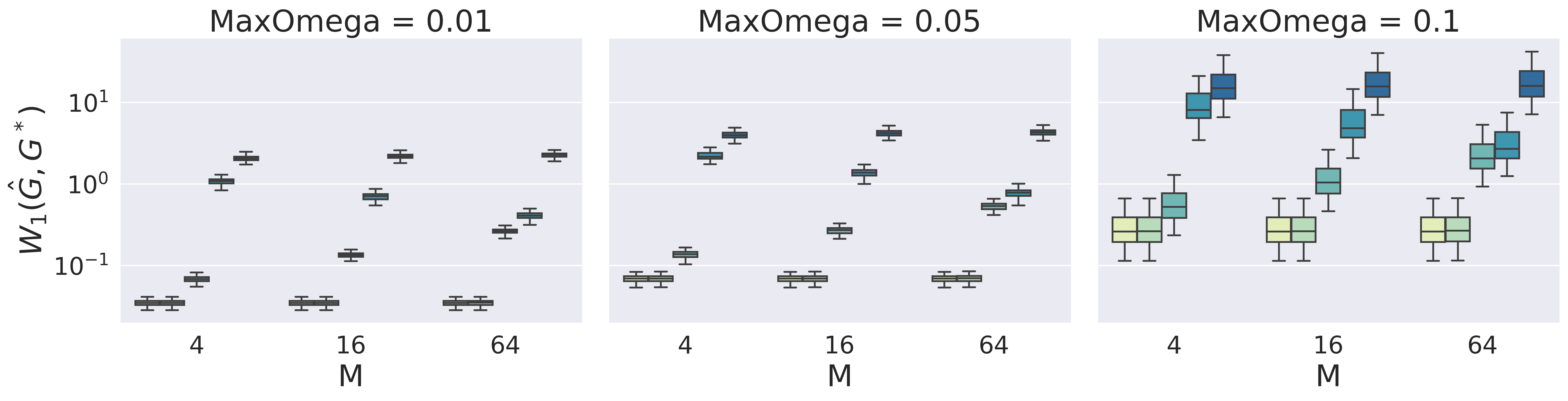
(a) Transportation distance $W_{1}$

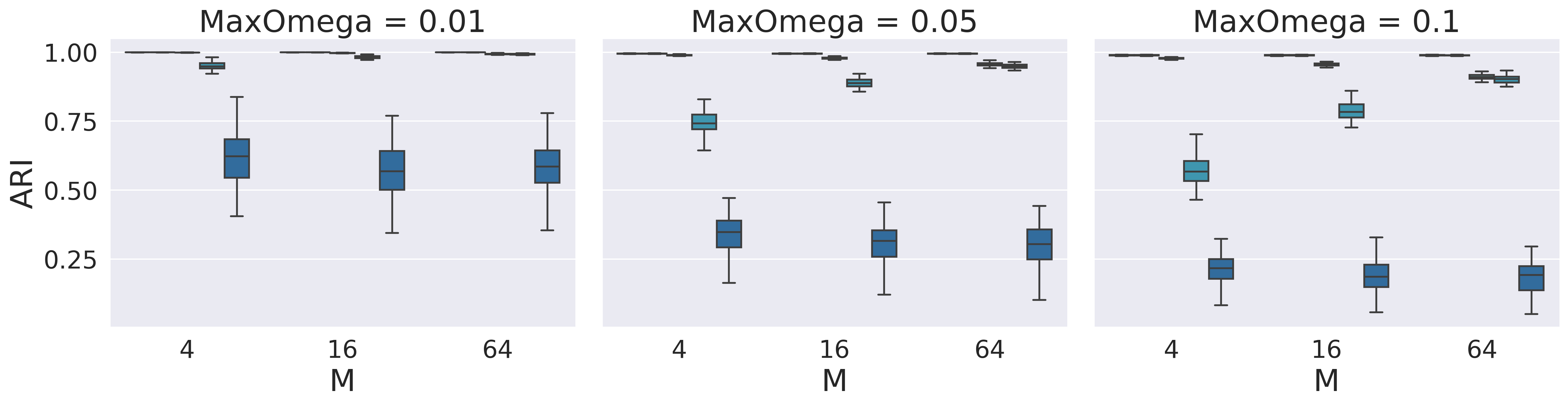
(b) ARI

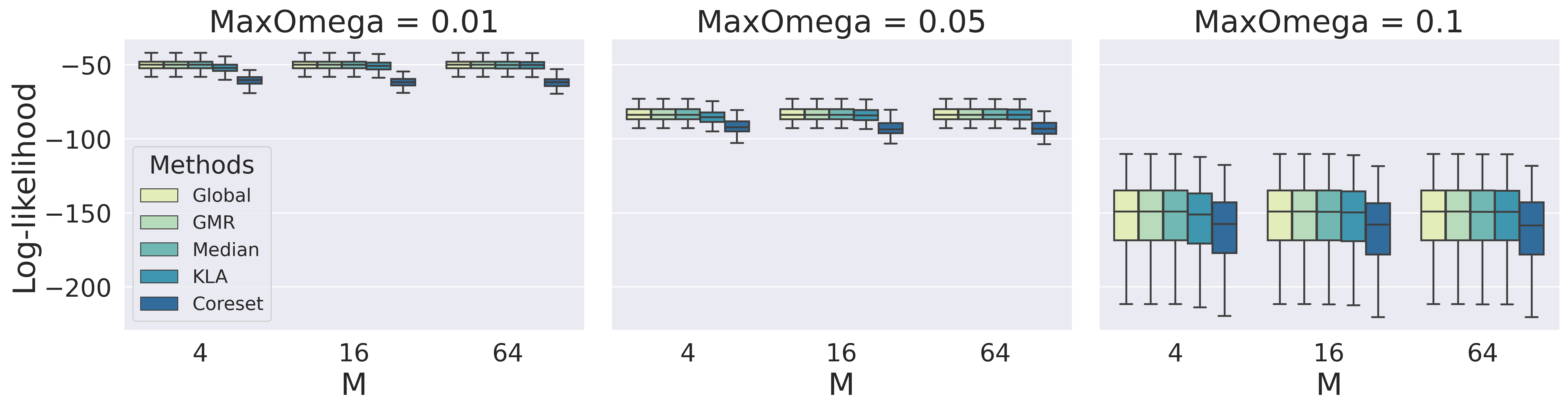
(c) Log-likelihood

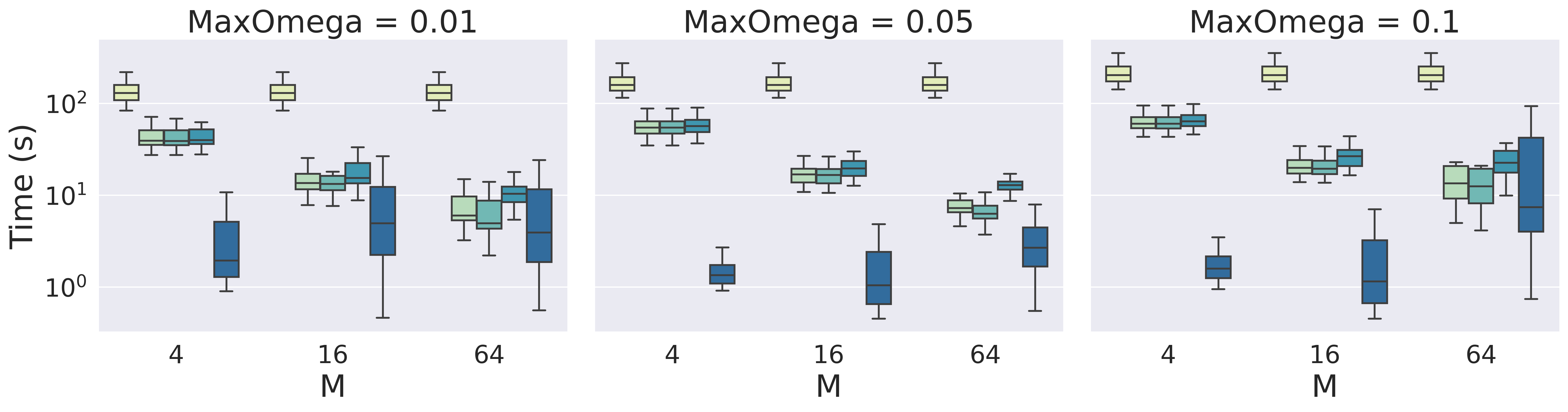
(d) Computational time

Figure 1: Comparison of Global, Median, GMR, KLA, and Coreset estimators for learning of $50$-dimensional $5$-component mixture when sample size is $N=2^{21}$ for various number of local machines and degree of overlap.

In general, the $W_{1}$ distances increase, the ARIs and log-likelihood decrease as the degree of overlapping increases. Our GMR estimator has comparable performance with the gold-standard global estimator in terms of both $W_{1}$ distance, ARI, and log-likelihood. The number of local machines has little influence on its performance. The KLA has even worse performance than the median, but it does better as the number of local machines increases. This is because the total sample size at the central machine increases proportionally with the number of local machines. The median estimator does not perform well when the number of local machines increases, likely because of the decreased sample sizes on the local machines. The Coreset estimator is worse than the KLA and its performance gets worse as the number of local machines increases, this is likely due to the information loss occurred during the merge of the coresets. The information loss increases as the number of merges increases.

In terms of computational time, all the aggregation approaches are more efficient than the global estimator and the Coreset estimator is computational fastest. However, the computational time for the Coreset estimator ignores the time for transmission, the actual computational time is therefore longer. The times increase as the degree of overlapping increases since more iterations are often needed. They also increase as the number of local machines increases. Because the aggregation times for GMR and the median estimators are often negligible, they use around (1/M)th of the time required by the global estimator. The aggregation step is more time-consuming for KLA, but it is still low. It has to fit the GMM an additional time on the pooled data generated from the local estimates.

In Figure 2, MaxOmega is fixed to $10\%$ and the number of local machines is set to $M=64$ for the same dataset. In general, Global, GMR, and Median perform better as the total sample size increases. The performance of Coreset gets worse as total sample size increases, this is because the coreset size is fixed to be $1000$ in all experiment and the precision of the approximation decreases as the total sample size increases. KLA performs slightly worse as the total sample size increases. Because the number of local machines is fixed, the larger sample size improves only the precision of the local estimates. For KLA the aggregation step is based on the observations generated from each local estimate; their built-in randomness is an important factor. The increased overall sample size is not particularly helpful. The other aspects of the simulation results are as expected.

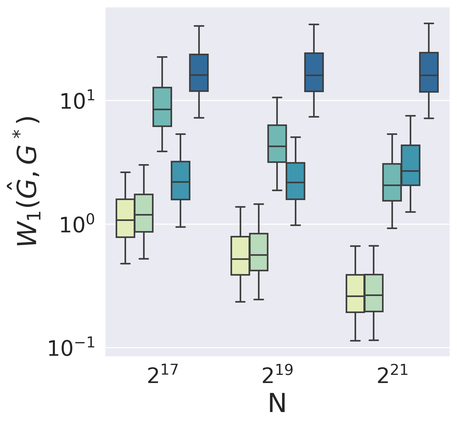
(a) $W_{1}$ distance

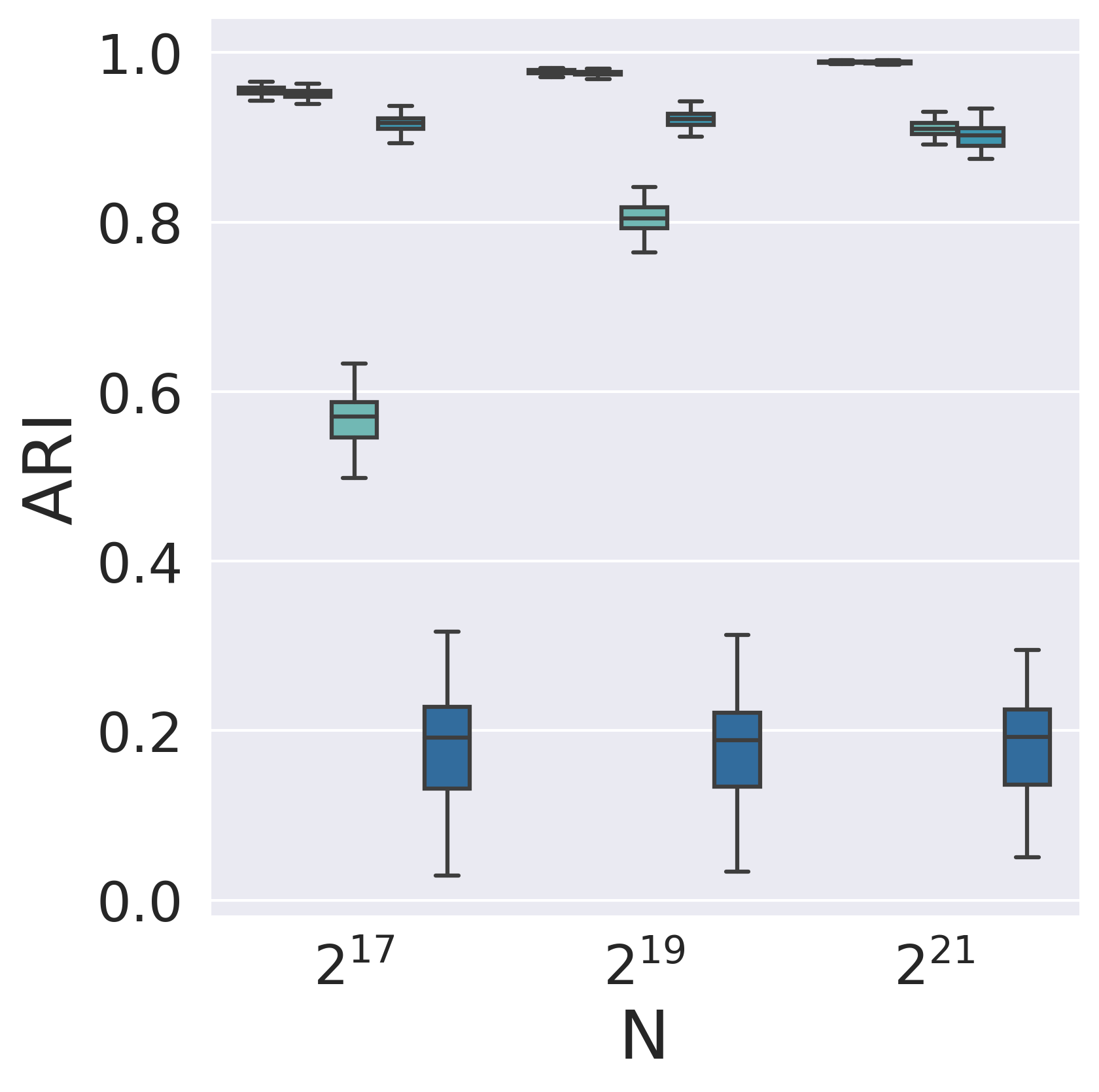
(b) ARI

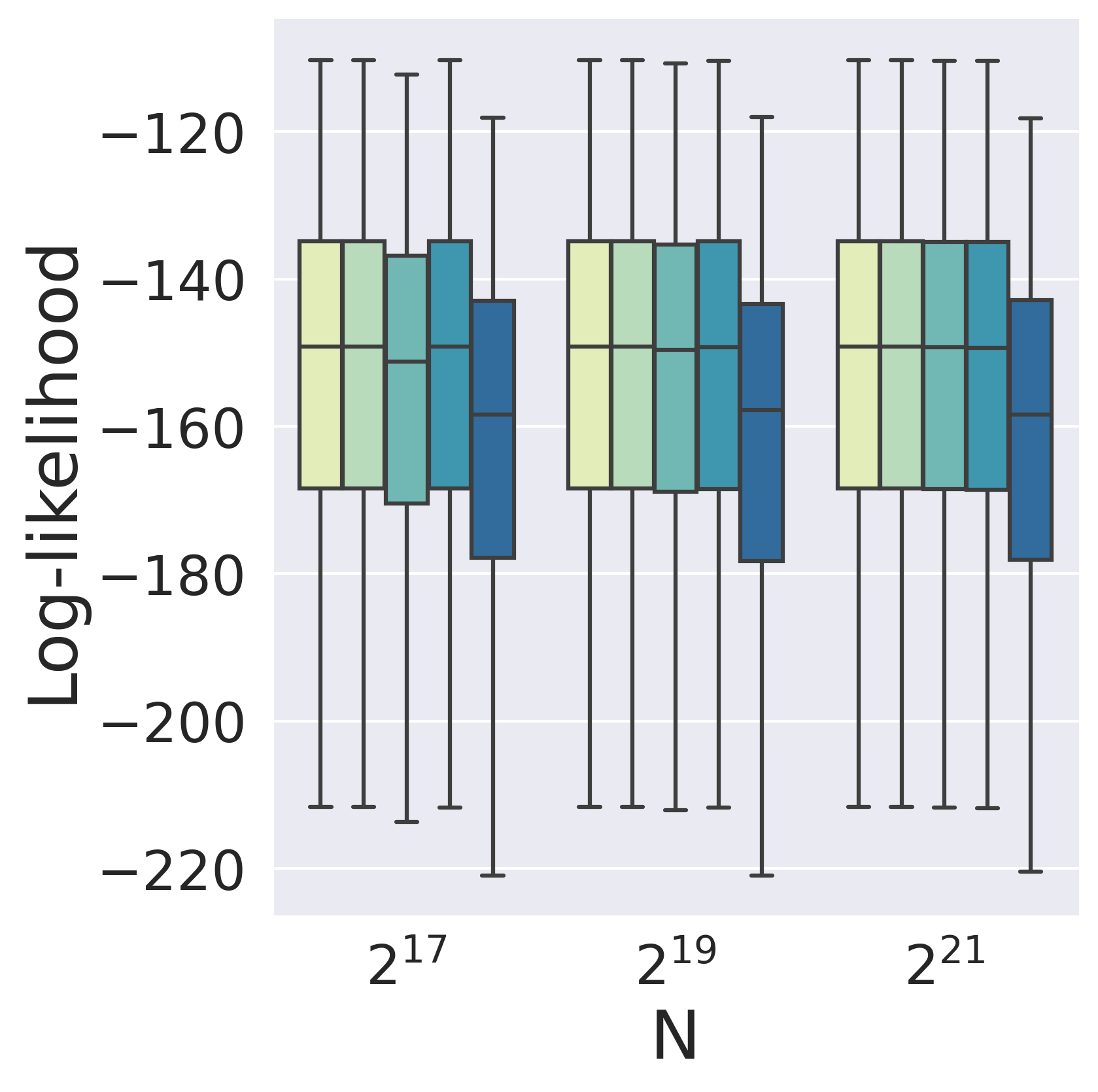
(c) Log-likelihood

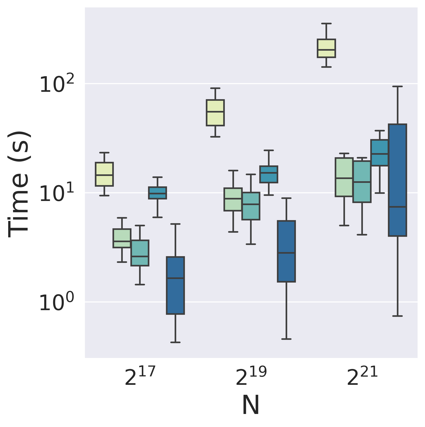
(d) Computational time

Figure 2: Comparison of Global, Median, GMR, KLA, and Coreset estimators when MaxOmega $=0.1$ and $M=64$ for learning of $50$-dimensional $5$-component mixture for various sample sizes.

In Appendix 8.3.1 we present simulation results for dimension $d=10,50$ combined with the order $K=5$, $10$, and $50$. Since the performance of the Coreset estimator is not as good as the rest of the estimators in the simulation described above, we therefore do not compare it with the rest of the estimators in this experiment. The general conclusions are similar in terms of the statistical efficiency. The local machine may take longer when $d=50$, $K=50$, and MaxOmega $\geq 5\%$.

7.3 Real Dataset

We compare the performance of the five estimators on large scale public datasets in Section 7.3.1. In Section 7.3.2, we show the performance of these five estimators on clustering the handwritten digits. In Section 7.3.3, we show an example of using the distributed learning for the application of clustering in large scale spatio-temporal data.

7.3.1 Public Datasets

We conduct the experiments on the public datasets that are widely used for learning Gaussian mixtures at scale. The following datasets are used in Lucic et al. (2017) and Jaini and Poupart (2016).

1. MAGIC04. This is a simulated dataset to classify gamma particles in the upper atmosphere, which contains $19,020$ observations in a $10$-dimensional space. We fit a mixture of order $K=10$ on this dataset. The dataset is publicly available at UCI machine learning repository.

2. MiniBooNE. The dataset is taken from the MiniBooNE experiment that is used to distinguish electron neutrinos from muon neutrinos. The dataset is publicly available at UCI machine learning repository. The dataset contains $130,065$ observations in a $50$-dimensional space. We fit a mixture of order $K=10$ on the dataset.

3. KDD. This dataset is used in Lucic et al. (2017) which contains $145751$ observations in a $74$-dimensional space for predicting the protein types. We fit a mixture of order $K=10$. The KDD dataset is available at https://kdd.org/kdd-cup/view/kdd-cup-2004/Data.

4. MSYP. The dataset is used to predict the release year of a song from audio features. There are $515,345$ instances in $90$-dimensional space. Following Lucic et al. (2017), we consider the top $25$ principal components and fit a mixture with order $K=50$. The dataset is publicly available at UCI machine learning repository.

For the first three datasets, we split the dataset onto $M=4$ local machines completely at random. Since the last datasets have the largest number of observations and the order of the mixture is high, we split the dataset onto $M=16$ local machines. The random split of the dataset is repeated for $R=100$ times for each split-and-conquer learning method. The size of the generated sample and coreset size are set to $1000$ in MAGIC04, for the rest of the datasets, this value is set to $10000$.

We report the median and the IQR of the value of the log-likelihood per observation evaluated at the learned mixing distribution based on the full dataset over $100$ repetitions in Table 1. When evaluating the log-likelihood function on MiniBooNE dataset with KLA and Coreset estimator, there is a numerical underflow problem due to the extreme small size of the log-likelihood value, we therefore remove these observations and compute the log-likelihood per value based on the rest of the observations. As a result, the upper bound of the log-likelihood value is given in the table. The relative performance of these estimators on the dataset is the same as that on the simulated dataset. It can be seen from the table that our proposed GMR approach is almost as good as the global estimator and is better than other split-and-conquer learning approaches on all datasets.

Table 1: The median log-likelihood per observation with IQR in parentheses.

Dataset	$N$	$d$	$K$	$M$	Global	GMR	Median	KLA	Coreset
MIGIC04	19020	10	10	4	-24.15	-24.30(0.07)	-26.60(0.05)	-26.73(0.07)	-27.16(0.55)
MiniBooNE	130065	50	10	4	-19.46	-22.00(0.53)	-24.60(0.32)	$\leq$-21.96(0.89)	$\leq$-25.11(3.21)
KDD	145751	74	10	4	-221.80	-223.25(0.42)	-232.93(8.02)	-235.00(8.96)	-374.43(193.58)
MSYP	515345	25	50	16	-166.56	-167.05(0.04)	-171.10(0.04)	-170.72(0.01)	-181.64(1.78)

The computational time of each method is given in Table 2, all the split-and-conquer learning methods can save a significant amount of time. For the MSYP dataset, the split-and-conquer methods save as least 10 times time than the global estimator. The Coreset estimator takes the shortest time. When the dimension of the mixture and the components of the mixture increases, the aggregation time of our proposed approach also increases but is still shorter than the KLA method.

Table 2: The median computational time in seconds with IQR in parentheses.

Dataset	$N$	$d$	$K$	$M$	Global	GMR	Median	KLA	Coreset
MIGIC04	19020	10	10	4	19.3	7.0(3.2)	6.7(3.2)	10.2(3.1)	2.2(0.6)
MiniBooNE	130065	50	10	4	346.9	313.1(162.6)	313.2(162.6)	511.3(213.2)	26.6(64.3)
KDD	145751	74	10	4	1033.9	544.4(309.5)	543.0(310.0)	706.0(290.3)	4.3(64.0)
MSYP	515345	25	50	16	67048.8	2611.6(474.0)	1777.5(511.2)	5515.9(1629.7)	67.4(12.6)

7.3.2 NIST Handwritten-Digit Dataset

The finite GMM is often used for model-based clustering (Friedman et al., 2001; Fraley and Raftery, 2002, Chapter 14.3), which requires the learning of a mixture from the data. When the dataset is large and/or distributed over local machines, split-and-conquer approaches such as our proposed GMR become useful. In this section, we demonstrate the use of the GMR method on the famous NIST dataset for character recognition (Grother and Hanaoka, 2016). We use the second edition, named by_class.zip . It consists of around 4M images of handwritten digits and characters (0–9, A–Z, and a–z) from different writers. This experiment focuses on the digits, and we still refer to it as the NIST dataset. The images of the digits are in directories 30–39. According to the user guide, the images in the train_30 to train_39 and hsf_4 folders are used as the training and test sets respectively. The numbers of training images for each digit are listed in the following table:

Table 3: The numbers of training images for each digit in NIST dataset.

Digits	0	1	2	3	4	5	6	7	8	9
Training	34803	38049	34184	35293	33432	31067	34079	35796	33884	33720
Test	5560	6655	5888	5819	5722	5539	5858	6097	5695	5813

Each image is a $128\times 128$ pixel grayscale matrix whose entries are real values between $0$ and $1$ that record the darkness of the corresponding pixels. A darker pixel has a value closer to $1$. Following the common practice, we first trained a $5$-layer convolutional neural network and reduced each image to a $d=50$ feature vector of real values. The details of the neural network for the dimension reduction are given in Appendix 8.3.2. A naïve approach to building a classifier is to regard the features of each digit as a random sample from a distinct Gaussian. The pooled data is therefore a sample from a $10$-component finite GMM. We may learn this model based on the whole dataset or through split-and-conquer approaches.

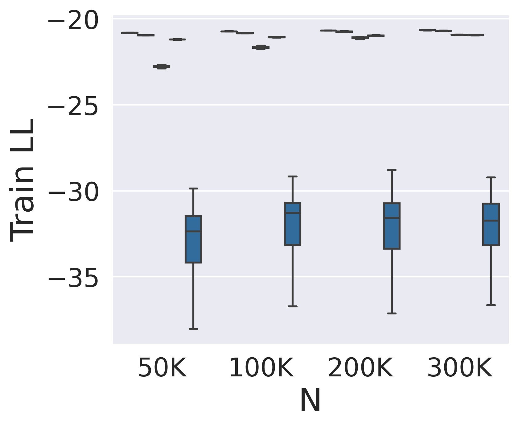
(a) Training LL

(b) Test LL

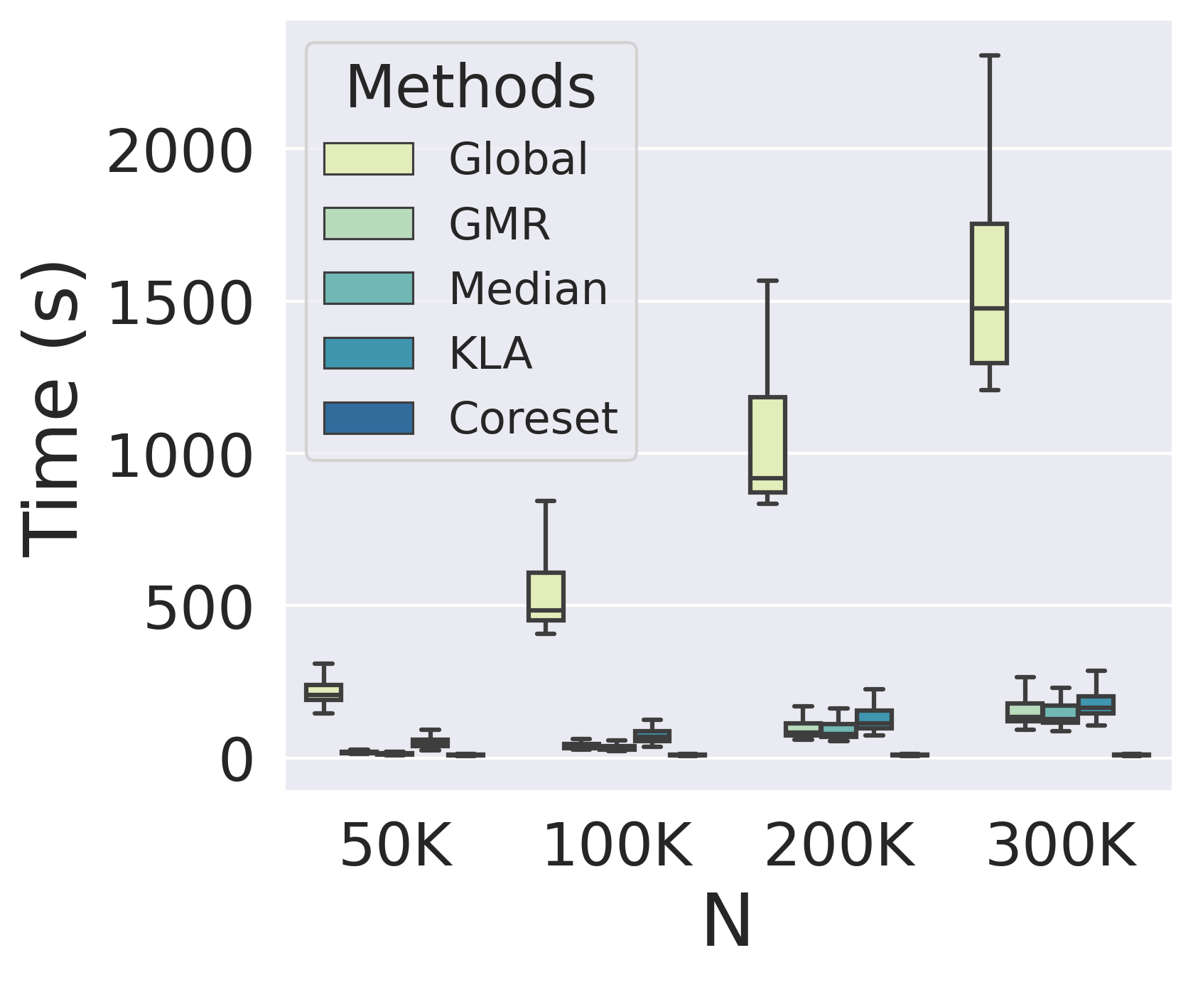
(c) Computational time

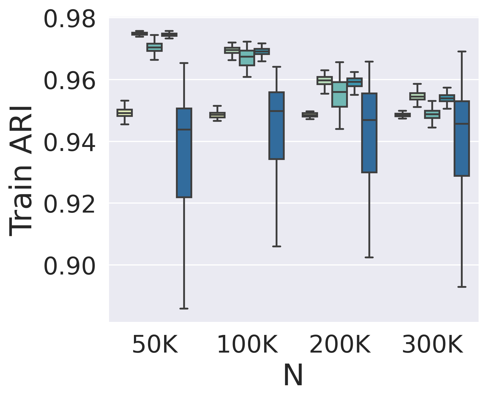
(d) Training ARI

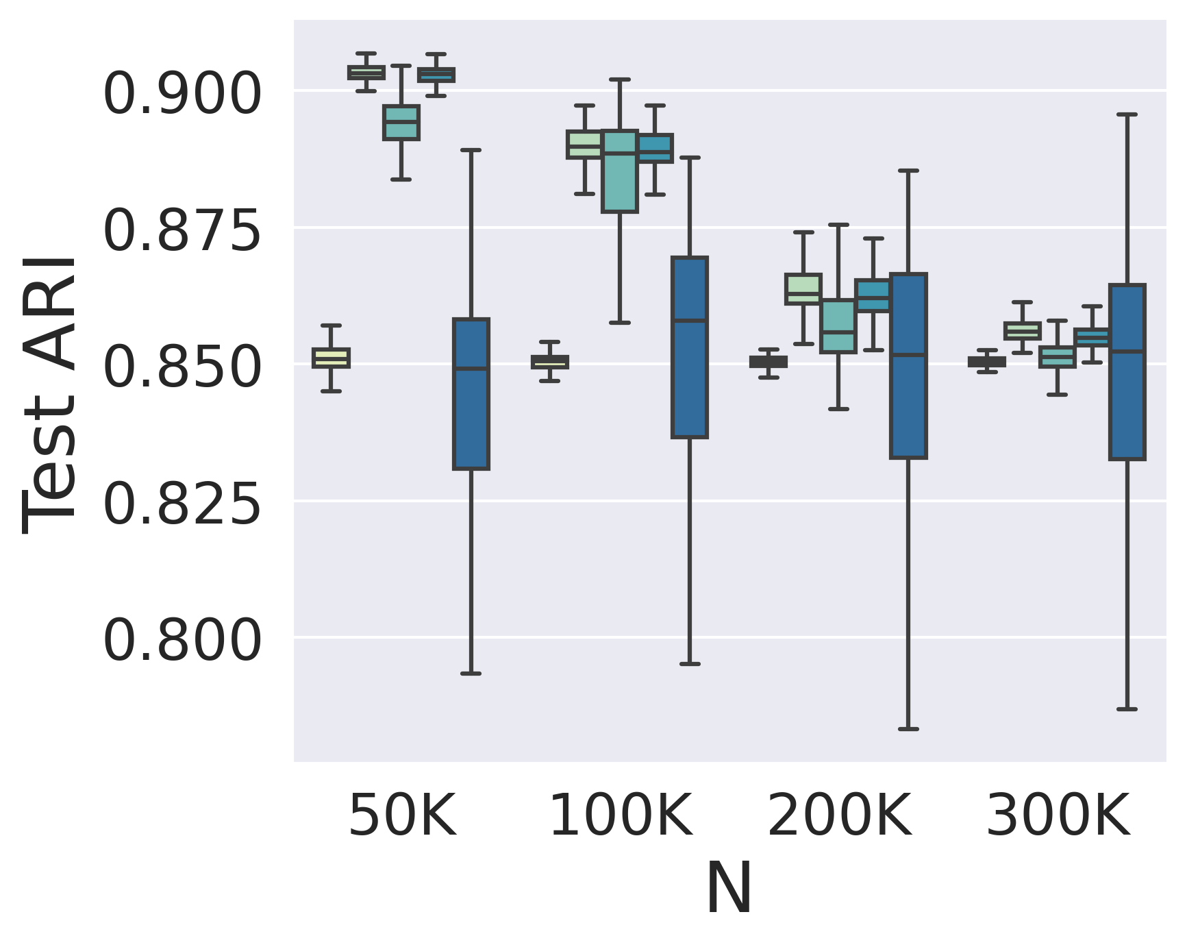
(e) Test ARI

Figure 3: Performance of split-and-conquer approaches for learning of $10$-component Gaussian mixture on $50$-dimensional space for NIST digit classification.

We randomly select $R=100$ datasets of size $N=50,000$ from the training set. Each dataset is then randomly partitioned into $M=10$ subsets. We obtain global, GMR, Median, KLA, and Coreset estimates for a $10$-component GMM on each dataset. The size of the generated sample for the KLA method and the coreset size in the Coreset method are both set to be $3000$. This experiment was also carried out with the sample sizes $N=100K$, $200K$, and $300K$. These mixture estimates are then used to cluster images of handwritten digits in the training and test sets. To assess the performance of different estimators, we compute the log-likelihood based on the training dataset and the test dataset. To compare the performance of these estimators for clustering, we compute the ARI between the true label of the image and the predicted label based on (19). Figures 3(a) and 3(b) respectively gives the boxplots of the log-likelihood based on the training set and the log-likelihood based on the test set. The boxplots of the ARI on the training set and the test set are given in Figure 3(d) and Figure 3(e).

In terms of the likelihood value, our method gives the highest log-likelihood among all split-and-conquer approaches and the Coreset estimators is the worst. When the total sample size is small, the Median estimator is worse than the KLA estimator and their difference becomes smaller as the total sample size increases. This is because the local sample size increases as the total sample size increases. When the total sample size is $300K$, the number of samples used to fit the local models and the samples generated to fit the aggregated model in the KLA approach are the same, it can be seen from the figure that the log-likelihood value of Median estimator and the KLA estimator are about the same.

In terms of the performance of the estimators for the purpose of clustering, surprisingly, the global estimator performs noticeably worse than the the split-and-conquer approaches although the global estimator has the highest log-likelihood value. A likely explanation is that the 10-component finite GMM is a working model rather than a true model, whereas true models are used in simulated data. This eliminates the advantage of the global estimator. This can also be seen that an increased total sample size $N$ does not lead to an improved fit in general. The ARIs get smaller as the total sample size increases, this is likely that we are more and more confident that the model is not accurate as more and more data comes in. Nevertheless, our method has the best performance in every case. It has the highest average ARI values and smaller variations.

Figure 3(c) shows that in terms of computational time, all split-and-conquer approaches saves the computational time. The Coreset estimator is the most efficient, the GMR and median estimators takes slightly longer and the KLA takes the longest time.

7.3.3 Atmospheric Data Analysis

We follow Chen et al. (2013) and apply our GMR approach to fit a finite GMM to an atmospheric dataset named CCSM run cam5.1.amip.2d.001. These data were created by computer simulation based on Community Atmosphere Model version 5 (CAM5). The dataset contains daily observations of multiple atmospheric variables between the years 1979 and 2005 over 192 longitudes (lon), 288 latitudes (lat), and 30 vertical altitude levels (lev). Our analysis only include variables: the moisture content (Q), temperature (T), and vertical velocity ($\Omega$, OMEGA) of the air.

For ease of comparison, we analyze only observations in December, January, and February, i.e., winter in the northern hemisphere. The number of days is thus 2430, and the restriction reduces the variation in the dataset. At each surface location, we filter out non-wet days (less than $1$ mm of daily precipitation) and focus on days with precipitation above the 95th wet-day percentile. This step reduces the number of observations at each location, not necessarily evenly. The analysis aims to cluster the locations according to the multivariate variable of dimension $d=91$: $30\mbox{ lev}\times\mbox{ \{Q, T, $\Omega$\}}$ plus the daily precipitation (PRECL) at the surface. Following Chen et al. (2013), we fit a finite GMM of order $K=4$. They suggest that this model is helpful in identifying modes of extreme precipitation in 3D atmospheric space over a few atmospheric variables.

After this preprocessing, the dataset still takes about 3 GB of memory, so we cannot learn a global mixture in a reasonable time. We partition the dataset evenly into $M=128$ subsets and apply our GMR approach with the same numerical strategies as in the NIST experiments. For comparison, we also aggregate the local estimates by the KLA with $500$ observations generated from each local estimate.

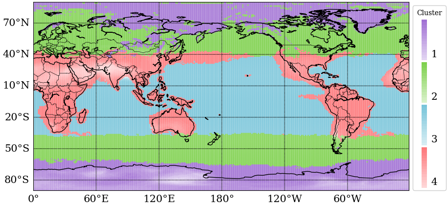
Figure 4: Surface locations colored by clusters. Within each cluster, the darker the color, the more wet days at that location.

Once a finite GMM has been learned, we cluster the observations based on (19). Each combination of day and surface location is clustered into one of four subpopulations. To visualize the clusters, we further allocate each surface location to the cluster in which it belongs on most days. Figure 4 shows these four clusters represented by different colors. Visually, the GMR clusters clearly separate the frigid, temperate, and tropical zones as well as the continental and oceanic areas. The KLA results in similar clusters.

8 Discussion and Concluding Remarks

We have developed an effective split-and-conquer approach for the learning of finite GMMs. Our experiments show that it has good performance both statistically and computationally. We have focused on finite GMMs, but with some adjustment our approach could be applied to learning mixtures with other subpopulation distributions such as Gamma and Poisson.

We have ignored many potential issues. In particular, we assume that the order of the mixture is correctly specified and that datasets on different local machines are IID and have the same underlying distributions. Our method may be regarded as a first step toward more satisfactory solutions to these real-world problems.

Appendices

The appendix is organized as follows. Section 8.1 contains all left over technical details and proofs, Section 8.2 presents the pseudocode of our algorithm, and Section 8.3 provides additional details.

8.1 Proofs

8.1.1 Example 2: Technical Details

We will show that $\mbox{$\mathbb{D}$}(\bar{G}^{C})<\mbox{$\mathbb{D}$}(\bar{G})$ where

$$\mbox{$\mathbb{D}$}(G)=0.5\mbox{$\mathbb{W}$}^{2}_{D,2}(G_{1},G)+0.5\mbox{$\mathbb{W}$}^{2}_{D,2}(G_{2},G).$$

This result implies that $\bar{G}$ is not a barycenter. We stop short of proving that $\bar{G}^{C}$ is. The latter task is so tedious that we have it omitted.

Note that all transportation plans from $G_{1}$ and $G_{2}$ to the presumed barycenter $\bar{G}^{C}$ have the form

$$\begin{pmatrix}p&0.4-p\\ 0.4-p&0.2+p\end{pmatrix}\mbox{ and }\begin{pmatrix}p&0.6-p\\ 0.4-p&p\end{pmatrix},$$

respectively, for some $p$ between $0$ and $0.4$. These two matrices are bivariate probability mass functions with the marginal probability masses $(0.4,0.6)$ and $(0.6,0.4)$ as required. The cost functions may be presented as

$$\begin{pmatrix}c(-1,-1)&c(-1,2/3)\\ c(1,-1)&c(1,2/3)\end{pmatrix}=\begin{pmatrix}0&25/9\\ 4&1/9\end{pmatrix}.$$

It is clear that $p=0.4$ gives the optimal plans for transporting $G_{1}$ to $\bar{G}^{C}$ and $G_{2}$ to $\bar{G}^{C}$. With these plans in place, we can see that

$$\mbox{$\mathbb{D}$}(\bar{G}^{C})=0.5\mbox{$\mathbb{W}$}^{2}_{D,2}(G_{1},\bar{G}^{C})+0.5\mbox{$\mathbb{W}$}^{2}_{D,2}(G_{2},\bar{G}^{C})=1/3.$$

In comparison, the optimal transportation plan from $G_{1}$ to $\bar{G}$ is to move $0.1$ mass from $\phi_{1}$ to $\phi_{-1}$ with a total cost of $0.1\times 4=0.4$. Hence,

$$\mbox{$\mathbb{D}$}(\bar{G})=0.5\mbox{$\mathbb{W}$}^{2}_{D,2}(G_{1},\bar{G})+0.5\mbox{$\mathbb{W}$}^{2}_{D,2}(G_{2},\bar{G})=0.4>1/3.$$

That is, $\bar{G}$ is not a barycenter.

8.1.2 Proof of Theorem 5

Let $G^{*}=\operatorname*{arg\,inf}\{\mathcal{J}_{c}(G):G\in\mathbb{G}_{K}\}.$ Let the mixing weights of any $G\in\mathbb{G}_{K}$ be $\mathbf{v}(G)$, and let the subpopulations prescribed by $G$ be $\Phi_{\gamma}$. According to (14), we have

$$\mathbf{v}(G^{*})=\sum_{i}\pi_{i,\gamma}(G^{\star}),$$

which implies that $\mbox{\boldmath$\pi$}(G^{*})\in\Pi(\cdot,\mathbf{v}(G^{*}))$. Since $\mbox{\boldmath$\pi$}(G^{*})\in\Pi(\mathbf{w},\cdot)$ by (9), we also have that $\mbox{\boldmath$\pi$}(G^{*})\in\Pi(\mathbf{w},\mathbf{v}(G^{*}))$ or it is a valid transportation plan from $\bar{G}$ to $G^{*}$. Consequently,

$$\inf\{\mathcal{T}_{c}(G):G\in\mathbb{G}_{K}\}\leq\sum_{i,\gamma}\pi_{i\gamma}(G^{*})c(\Phi_{i},\Phi^{*}_{\gamma})=\mathcal{J}_{c}(G^{*})=\inf\{\mathcal{J}_{c}(G):G\in\mathbb{G}_{K}\},$$

with the last equality implied by the definition of $G^{*}$. This inequality implies that the left-hand side of (12) is less than its right-hand side.

Next, we prove that the inequality holds in the other direction. Let $G^{\dagger}=\inf\{\mathcal{T}_{c}(G):G\in\mathbb{G}_{K}\}$, the solution to the optimization on the left-hand side of (12). We denote the subpopulations prescribed by $G^{\dagger}$ as $\Phi_{\gamma}^{\dagger}$. Let

$$\mbox{\boldmath$\pi$}^{\dagger}=\operatorname*{arg\,inf}\big{\{}\sum_{i,\gamma}\mbox{\boldmath$\pi$}_{i\gamma}c(\Phi_{i},\Phi^{\dagger}_{\gamma}):\mbox{\boldmath$\pi$}\in\Pi(\mathbf{w},\mathbf{v}(G^{\dagger}))\big{\}},$$

which is the optimal transportation plan from $\bar{G}$ to this $G^{\dagger}$. Because of this, we have

$$\inf\{\mathcal{T}_{c}(G):G\in\mathbb{G}_{K}\}=\mathcal{T}_{c}(G^{\dagger})=\sum_{i,\gamma}\mbox{\boldmath$\pi$}^{\dagger}_{i\gamma}c(\Phi_{i},\Phi^{\dagger}_{\gamma})\geq\mathcal{J}_{c}(G^{\dagger})\geq\inf\{\mathcal{J}_{c}(G):G\in\mathbb{G}_{K}\}.$$

The last step holds because $\mbox{\boldmath$\pi$}^{\dagger}\in\Pi(\mathbf{w},\cdot)$. This completes the proof.

8.1.3 Proof of Theorem 7

(i). Clearly, we have $\mathcal{K}_{c}(G|G_{t})\geq\mathcal{J}_{c}(G)$ for all $G$ with equality holds at $G=G_{t}$. Hence,

$$\begin{split}\mathcal{J}_{c}(G_{t})&\geq\mathcal{J}_{c}(G_{t})-\{\mathcal{K}_{c}(G_{t+1}|G_{t})-\mathcal{J}_{c}(G_{t+1})\}\\ &=\mathcal{J}_{c}(G_{t+1})-\{\mathcal{K}_{c}(G_{t+1}|G_{t})-\mathcal{J}_{c}(G_{t})\}\\ &\geq\mathcal{J}_{c}(G_{t+1})-\{\mathcal{K}_{c}(G_{t}|G_{t})-\mathcal{J}_{c}(G_{t})\}\\ &=\mathcal{J}_{c}(G_{t+1}).\end{split}$$

This is the property that an MM-algorithm must have.

(ii). Suppose $G^{(t)}$ has a convergent subsequence leading to a limit $G^{*}$. Let this subsequence be $G^{(t_{k})}$. By Helly’s selection theorem (Van der Vaart, 2000), there is a subsequence $s_{k}$ of $t_{k}$ such that $G^{(s_{k}+1)}$ has a limit, say $G^{**}$. These limits, however, could be subprobability distributions. That is, we cannot rule out the possibility/measure that the total probability in the limit is below 1 by Helly’s theorem.

This is not the case under the theorem conditions. Let $\Delta>0$ be large enough such that

$$A_{1}=\{\Phi:c(\Phi_{i},\Phi)\leq\Delta,\mbox{for all subpopulations $\Phi_{i}$ of }\bar{G}\}$$

is not empty. With this $\Delta$, we define

$$A_{2}=\{\Phi:c(\Phi_{i},\Phi)>\Delta,\mbox{for all subpopulations $\Phi_{i}$ of }\bar{G}\}.$$

Suppose $G^{\dagger}$ has a subpopulation $\Phi^{\dagger}$ such that $c(\Phi_{i},\Phi^{\dagger})>\Delta$ for all $i$. Replacing this subpopulation in $G^{\dagger}$ by any $\Phi^{\dagger\dagger}\in A_{1}$ to form $G^{\dagger\dagger}$, we can see that for any $t$,

$$\mathcal{K}_{c}(G^{\dagger}|G^{(t-1)})>\mathcal{K}_{c}(G^{\dagger\dagger}|G^{(t-1)}).$$

This result shows that none of the subpopulations of $G^{(t)}$ are members of $A_{2}$. Otherwise, $G^{(t)}$ does not minimize $\mathcal{K}_{c}(G|G^{(t-1)})$ at the $t$th iteration.

Note that the complement of $A_{2}$ is compact by condition (17). Consequently, the subpopulations of $G^{(t)}$ are confined to a compact subset. Hence, all limit points of $G^{(t)}$, including both $G^{*}$ and $G^{**}$, are proper distributions. By the monotonicity of the iteration:

$$\mathcal{J}_{c}(G^{(s_{k+1})})\leq\mathcal{J}_{c}(G^{(s_{k}+1)})\leq\mathcal{J}_{c}(G^{(s_{k})}).$$

Let $k\to\infty$, we get

$$\mathcal{J}_{c}(G^{**})=\mathcal{J}_{c}(G^{*}).$$ (20)

By the definition of the MM iteration, we have

$$\mathcal{K}_{c}(G^{(s_{k}+1)}|G^{(s_{k})})\leq\mathcal{K}_{c}(G|G^{(s_{k})}).$$

Let $k\to\infty$ and by the continuity of $\mathcal{K}_{c}(\cdot|\cdot)$, we get

$$\mathcal{K}_{c}(G^{**}|G^{*})\leq\mathcal{K}_{c}(G|G^{*}).$$

Hence, $G^{**}$ is a solution to $\min\mathcal{K}_{c}(G|G^{{t})})$ when $G^{(t)}=G^{*}$. Namely,, we have $\mathcal{K}_{c}(G^{**}|G^{*})=\mathcal{K}_{c}(G^{(t+1)}|G^{*})$. With the help of (20), it further implies

$$\mathcal{J}_{c}(G^{**})=\mathcal{J}_{c}(G^{(t+1)})=\mathcal{J}_{c}(G^{*})$$

when $G^{(t)}=G^{*}$. This shows that iteration from $G^{(t)}=G^{*}$ does not make $\mathcal{J}_{c}(G^{(t+1)})$ smaller than $\mathcal{J}_{c}(G^{(t)})$. Hence, $G^{*}$ is a stationary point of the MM iteration. This is conclusion (ii) and we have completed the proof.

8.1.4 Proof of Theorem 9

Recall that the local estimators $\hat{G}_{m},m\in[M]$ are strongly consistent for $G^{*}$ when the order $K$ of $G^{*}$ is known. Clearly, this implies that the aggregate estimator $\bar{G}\to G^{*}$ and $\mathcal{T}_{c}(\bar{G},G^{*})\to 0$ almost surely. That is, other than a probability 0 event in the probability space $\Omega$ on which the random variables are defined, convergence holds. Furthermore, each support point of $\bar{G}$ must converge to one of those of $G^{*}$. The total weights of the support points of $\bar{G}$ converging to the same support of $G^{*}$ must converge to the corresponding weight of $G^{*}$. Without loss of generality, assume $\mathcal{T}_{c}(\bar{G},G^{*})\to 0$ holds at all $\omega\in\Omega$ without a zero-probability exception.

By definition, $\bar{G}^{R}$ has $K$ support points. We also notice that

$$\mathcal{T}_{c}(\bar{G},\bar{G}^{R})\leq\mathcal{T}_{c}(\bar{G},G^{*})\to 0.$$ (21)

Suppose that $\bar{G}^{R}$ does not converge to $G^{*}$ at some $\omega\in\Omega$. One possibility is that the smallest mixing weight of $\bar{G}^{R}$ (or a subsequence thereof) goes to zero as $N\to\infty$. In this case, $\bar{G}^{R}$ has $K-1$ or fewer meaningful support points. Since the support points of $\bar{G}$ are in an infinitesimal neighborhood of those of $G^{*}$, one of them must be a distance away from any of the support points of $\bar{G}^{R}$. Therefore, by Condition 4, the transportation cost of this support point is larger than a positive constant not depending on $N$. The positive transportation cost implies that $\mathcal{T}_{c}(\bar{G},\bar{G}^{R})\not\to 0$, which contradicts (21).

The next possibility is that the smallest mixing weight of $\bar{G}^{R}$ does not go to zero. In this case, there is a subsequence such that all the mixing weights converge to positive constants. Without loss of generality, all the mixing weights simply converge to positive constants as $N\to\infty$. If there is a subsequence of support points of $\bar{G}^{R}$ that is at least $\epsilon$-distance away from any of the support points of $G^{*}$, then the transportation cost from $\bar{G}$ to this support point will be larger than a positive constant not depending on $N$. This again leads to a contradiction to (21).

The final possibility is that $\bar{G}^{R}$ (or a subsequence thereof) has a proper limit, say $G^{**}\neq G^{*}$. If so, $\mathcal{T}_{c}(\bar{G},\bar{G}^{R})\to\mathcal{T}_{c}(G^{*},G^{**})\neq 0$, contradicting (21).

We have exhausted all the possibilities. Hence, the consistency claim is true.

8.1.5 Proof of Theorem 10

We start with a few rate conclusions. Let $\Phi_{mk}$ be the $k$th subpopulation learned at local machine $m$ and $w_{mk}$ be its mixing weight. Note that we do not put a “hat” on them for notation simplicity. According to Lemma 8 on the rate of convergence of the pMLE at local machines, these subpopulations can be arranged so that for all $m\in[M]$ and $k\in[K]$, we have

$$\|\Phi_{mk}-\Phi^{*}_{k}\|=O_{p}(N^{-1/2}),~{}~{}~{}\sum_{m}\lambda_{m}w_{mk}-w^{*}_{k}=O_{p}(N^{-1/2}).$$

By C5, the first rate conclusion above implies

$$\max\{c(\Phi_{mk},\Phi^{*}_{k}):k\in[K]\}=O_{p}(N^{-1}).$$

For each $k$, let $\widetilde{w}_{k}=\sum_{m=1}^{M}\lambda_{m}w_{mk}$ and $\widetilde{\Phi}_{k}$ be the local barycenter of $\Phi_{mk}$, $m\in[M]$:

$$\widetilde{\Phi}_{k}=\operatorname*{arg\,min}\{\Phi:\sum_{m=1}^{M}\lambda_{m}w_{mk}c(\Phi_{mk},\Phi)\}.$$

By the rate conclusions given earlier, we have $\widetilde{w}_{k}=w^{*}_{k}+O_{p}(N^{-1/2})$ for $k\in[K]$. By C5, we must also have

$$\|\widetilde{\Phi}_{k}-\Phi^{*}_{k}\|=O_{p}(N^{-1/2})$$

and $\mathcal{T}_{c}(\bar{G},\widetilde{G})=o_{p}(N^{-1})$. This $\bar{G}^{R}$ is given by $\widetilde{G}$, then the rate conclusion of the theorem is proved.

Next, we show that the GMR $\bar{G}^{R}$ is given by $\widetilde{G}$ asymptotically. By theorem conditions, the true subpopulations $\Phi^{*}_{k}$ are all distinct. Hence, by condition C4, we have

$$\min\{c(\Phi^{*}_{k},\Phi^{*}_{k^{\prime}}):k\neq k^{\prime}\in[K]\}>0.$$

Thus, if the subpopulations of $\bar{G}^{R}$ is not in an $o_{p}(1)$ neighbourhood of one of $\Phi^{*}_{k}$ even though everyone of $\bar{G}$ is, the transport cost to this subpopulation from any subpopopulation of $\bar{G}$ exceeds a positive constant in probability. This contradicts

$$\mathcal{T}_{c}(\bar{G},\bar{G}^{R})\leq\mathcal{T}_{c}(\bar{G},\widetilde{G})=o_{p}(N^{-1}).$$ (22)

This implies, all subpopulations of $\bar{G}^{R}$ are within $o_{p}(1)$ neighbourhood of one of $\Phi^{*}_{k}$. Denote these subpopulations as $\bar{\Phi}_{k}^{R}$ The optimal plan must transport $\Phi_{mk}$ to $\bar{\Phi}_{k}^{R}$, otherwise the total transport cost exceeds a positive constant in probability which again contradicts (22). Since $\bar{G}^{R}$ minimizes the transport cost, we must have $\bar{\Phi}_{k}^{R}=\widetilde{\Phi}_{k}$, the local barycenter. These conclusions imply that GMR $\bar{G}^{R}=\widetilde{G}$ with probability approaching to 1. Consequently, the rates of convergence of $\widetilde{w}_{k},\widetilde{\Phi}_{k}$ extend to those of $\bar{G}^{R}$ and this completes the proof.

8.1.6 KL-divergence satisfies C5

Let $\mbox{\boldmath$\mu$}_{1},\mbox{\boldmath$\Sigma$}_{1}$ and $\mbox{\boldmath$\mu$}_{2},\mbox{\boldmath$\Sigma$}_{2}$ be the parameters of $\Phi_{1}$ and $\Phi_{2}$. It is known that

$$2D_{\text{KL}}(\Phi_{1}\|\Phi_{2})=\log\{\text{det}(\mbox{\boldmath$\Sigma$}_{2})/\text{det}(\mbox{\boldmath$\Sigma$}_{1})\}+\text{tr}(\mbox{\boldmath$\Sigma$}_{2}^{-1}\mbox{\boldmath$\Sigma$}_{1}-\mathbf{I}_{d})+(\mbox{\boldmath$\mu$}_{2}-\mbox{\boldmath$\mu$}_{1})^{\tau}\mbox{\boldmath$\Sigma$}_{2}^{-1}(\mbox{\boldmath$\mu$}_{2}-\mbox{\boldmath$\mu$}_{1}).$$

Assume both $\Phi_{1}$ and $\Phi_{2}$ are in a small neighborhood of $\Phi$ whose covariance matrix $\Sigma$ is positive definite. Hence, eigenvalues of $\mbox{\boldmath$\Sigma$}_{2}$ are in small neighborhood of these of $\Sigma$. Thus, there exists a positive constant $A_{1}$ such that the second term in $2D_{\text{KL}}(\Phi_{1}\|\Phi_{2})$ satisfies

$$A_{1}^{-1}\|\mbox{\boldmath$\mu$}_{2}-\mbox{\boldmath$\mu$}_{1}\|^{2}\leq(\mbox{\boldmath$\mu$}_{2}-\mbox{\boldmath$\mu$}_{1})^{\tau}\mbox{\boldmath$\Sigma$}_{2}^{-1}(\mbox{\boldmath$\mu$}_{2}-\mbox{\boldmath$\mu$}_{1})\leq A_{1}\|\mbox{\boldmath$\mu$}_{2}-\mbox{\boldmath$\mu$}_{1}\|^{2}$$ (23)

Let $\lambda_{1},\ldots,\lambda_{d}$ be eigenvalues of $\mbox{\boldmath$\Sigma$}_{2}^{-1/2}\mbox{\boldmath$\Sigma$}_{1}\mbox{\boldmath$\Sigma$}_{2}^{-1/2}$. Since both $\mbox{\boldmath$\Sigma$}_{1}$ and $\mbox{\boldmath$\Sigma$}_{2}$ are in a small neighborhood of $\Sigma$, we have $\lambda_{1},\ldots,\lambda_{d}$ all close to 1.

$$\log\{\text{det}(\mbox{\boldmath$\Sigma$}_{2})/\text{det}(\mbox{\boldmath$\Sigma$}_{1})\}+\text{tr}(\mbox{\boldmath$\Sigma$}_{2}^{-1}\mbox{\boldmath$\Sigma$}_{1}-\mathbf{I}_{d})=\sum_{j=1}^{d}\{(\lambda_{j}-1)-\log\lambda_{j}\}.$$

Note that $(\lambda-1)-\log\lambda$ is a convex function with its minimum attained at $\lambda=1$ at which point its second derivative equals 1. Hence, there exists an $A_{2}>0$ such that

$$A_{2}^{-1}(\lambda-1)^{2}\leq(\lambda-1)-\log\lambda\leq A_{2}(\lambda-1)^{2}.$$

We have therefore shown that

$$A_{2}^{-1}\sum_{j=1}^{d}(\lambda_{j}-1)^{2}\leq\log\{\text{det}(\mbox{\boldmath$\Sigma$}_{2})/\text{det}(\mbox{\boldmath$\Sigma$}_{1})\}+\text{tr}(\mbox{\boldmath$\Sigma$}_{2}^{-1}\mbox{\boldmath$\Sigma$}_{1}-\mathbf{I}_{d})\leq A_{2}\sum_{j=1}^{d}(\lambda_{j}-1)^{2}.$$ (24)

We now connect the bound with Frobenius norm.

For a positive definite matrix $\Sigma$, it is easy to see that $\|\mbox{\boldmath$\Sigma$}-\mathbf{I}_{d}\|_{F}^{2}=\sum_{j=1}^{d}(\sigma_{j}-1)^{2}$, where $\sigma_{1},\sigma_{2},\ldots,\sigma_{d}$ are eigenvalues of $\Sigma$. Frobenius norm also has sub-multiplicative property

$$\|\mbox{\boldmath$\Sigma$}_{1}\mbox{\boldmath$\Sigma$}_{2}\|_{F}\leq\|\mbox{\boldmath$\Sigma$}_{1}\|_{F}\|\mbox{\boldmath$\Sigma$}_{2}\|_{F}.$$

Applying the sub-multiplicative property in our context, we get

$$\|\mbox{\boldmath$\Sigma$}_{1}-\mbox{\boldmath$\Sigma$}_{2}\|^{2}_{F} \leq ~{}\|\mbox{\boldmath$\Sigma$}_{2}^{1/2}\|^{4}_{F}~{}\|\mbox{\boldmath$\Sigma$}_{2}^{-1/2}\mbox{\boldmath$\Sigma$}_{1}\mbox{\boldmath$\Sigma$}_{2}^{-1/2}-\mathbf{I}_{d}\|^{2}_{F}$$

$$\leq A_{3}~{}\|\mbox{\boldmath$\Sigma$}_{2}^{-1/2}\mbox{\boldmath$\Sigma$}_{1}\mbox{\boldmath$\Sigma$}_{2}^{-1/2}-\mathbf{I}_{d}\|^{2}_{F}$$

$$= A_{3}~{}\sum_{j=1}^{d}(\lambda_{j}-1)^{2}$$

for some local positive constant $A_{3}>\|\mbox{\boldmath$\Sigma$}^{1/2}\|^{4}_{F}$, as both matrices are in a small neighborhood of $\Sigma$. Similarly, we have

$$\sum_{j=1}^{d}(\lambda_{j}-1)^{2} = \|\mbox{\boldmath$\Sigma$}_{2}^{-1/2}\mbox{\boldmath$\Sigma$}_{1}\mbox{\boldmath$\Sigma$}_{2}^{-1/2}-\mathbf{I}_{d}\|^{2}_{F}$$

$$= \|\mbox{\boldmath$\Sigma$}_{2}^{-1/2}\{\mbox{\boldmath$\Sigma$}_{1}-\mbox{\boldmath$\Sigma$}_{2}\}\mbox{\boldmath$\Sigma$}_{2}^{-1/2}\|^{2}_{F}$$

$$\leq \|\mbox{\boldmath$\Sigma$}_{2}^{-1/2}\|^{4}_{F}~{}\|\mbox{\boldmath$\Sigma$}_{1}-\mbox{\boldmath$\Sigma$}_{2}\|^{2}_{F}$$

$$\leq A_{4}\|\mbox{\boldmath$\Sigma$}_{1}-\mbox{\boldmath$\Sigma$}_{2}\|^{2}_{F}.$$

for some positive constant $A_{4}$. This leads to

$$\|\mbox{\boldmath$\Sigma$}_{1}-\mbox{\boldmath$\Sigma$}_{2}\|^{2}_{F}\geq A_{4}^{-1}\sum_{j=1}^{d}(\lambda_{j}-1)^{2}.$$

Let $A=2\max\{A_{1},A_{2},A_{3},A_{4}\}$. Applying (23) and (24), we have

$$A^{-1}\{\|\mbox{\boldmath$\mu$}_{1}-\mbox{\boldmath$\mu$}_{2}\|^{2}+\|\mbox{\boldmath$\Sigma$}_{1}-\mbox{\boldmath$\Sigma$}_{2}\|^{2}_{F}\}\leq D_{\text{KL}}(\Phi_{1}\|\Phi_{2})\leq A\{\|\mbox{\boldmath$\mu$}_{1}-\mbox{\boldmath$\mu$}_{2}\|^{2}+\|\mbox{\boldmath$\Sigma$}_{1}-\mbox{\boldmath$\Sigma$}_{2}\|^{2}_{F}\}$$

when $\Phi_{1},\Phi_{2}$ are in a small neighborhood of $\Phi$, with $A$ being a positive constant depends on $\Phi$. This shows that the KL-divergence has property C5.

8.2 Algorithm

Algorithm 1 gives the pseudocode for the GMR estimator with the KL-divergence cost function.

Initialization: $\Phi_{\gamma}$, $\gamma\in[K]$

repeat

     for $\gamma\in[K]$ do

         for $i\in[MK]$ do

              Let

$$\pi_{i\gamma}=\begin{cases}w_{i}&\text{if}~{}\gamma=\operatorname*{arg\,min}_{\gamma^{\prime}}D_{\text{KL}}(\Phi_{i},\Phi_{\gamma^{\prime}})\\ 0&\text{otherwise}\end{cases}$$

         end for

         Let

$$\begin{split}\mbox{\boldmath$\mu$}_{\gamma}&=\sum_{i=1}^{MK}\{\pi_{i\gamma}/\pi_{\cdot\gamma}\}\mbox{\boldmath$\mu$}_{i}\\ \mbox{\boldmath$\Sigma$}_{\gamma}&=\sum_{i=1}^{MK}\{\pi_{i\gamma}/\pi_{\cdot\gamma}\}\{\mbox{\boldmath$\Sigma$}_{i}+(\mbox{\boldmath$\mu$}_{i}-\mbox{\boldmath$\mu$}_{\gamma})(\mbox{\boldmath$\mu$}_{i}-\mbox{\boldmath$\mu$}_{\gamma})^{\tau}\}\end{split}$$

     end for

until the value of the objective function $\sum_{i,\gamma}\pi_{i\gamma}D_{\text{KL}}(\Phi_{i},\Phi_{\gamma})$ converges

for $\gamma\in[K]$ do

     Let $v_{\gamma}=\sum_{i}\pi_{i\gamma}$

end for

Output: $\{(v_{\gamma},\mbox{\boldmath$\mu$}_{\gamma},\mbox{\boldmath$\Sigma$}_{\gamma}):\gamma\in[K]\}$

Algorithm 1 MM algorithm for GMR estimator with KL-divergence cost function

8.3 Additional Details

8.3.1 Additional Simulation Results

In this section, we present additional simulation results for $K=5,10,50$ and $d=10,50$. All the settings are as in Section 7.2. Figures 5–6 show the results for $N=2^{19}$ and $M=4$ with various combinations of $K$ and $d$. The panels in each figure are arranged so that the order of the mixture increases from left to right, and the dimension of the mixture increases from top to bottom.

Comparing panels within the same row in Figure 5, we note that the performance of all the estimators becomes worse as the order of the mixture increases in terms of $W_{1}$ distance. The panels within the same column in Figures 5 show that all the estimators become worse as the dimension of the mixture increases in terms of both performance measures.

Regardless, our estimator has performance comparable to that of the global estimator. In terms of the misclassification error, for the same degree of overlapping, the superiority of our estimator increases compared to the KL-averaging as the number of components and the dimension increase.

The computational costs of the local estimators are typically low, and this gives our method an added computational advantage. However, this advantage is not guaranteed: see the bottom right panel in Figure 6, where $d=50$, $K=50$, and the degree of overlapping is above $1\%$. There are many other factors at play. A more skillful implementation may lead to different conclusions on the computational time.

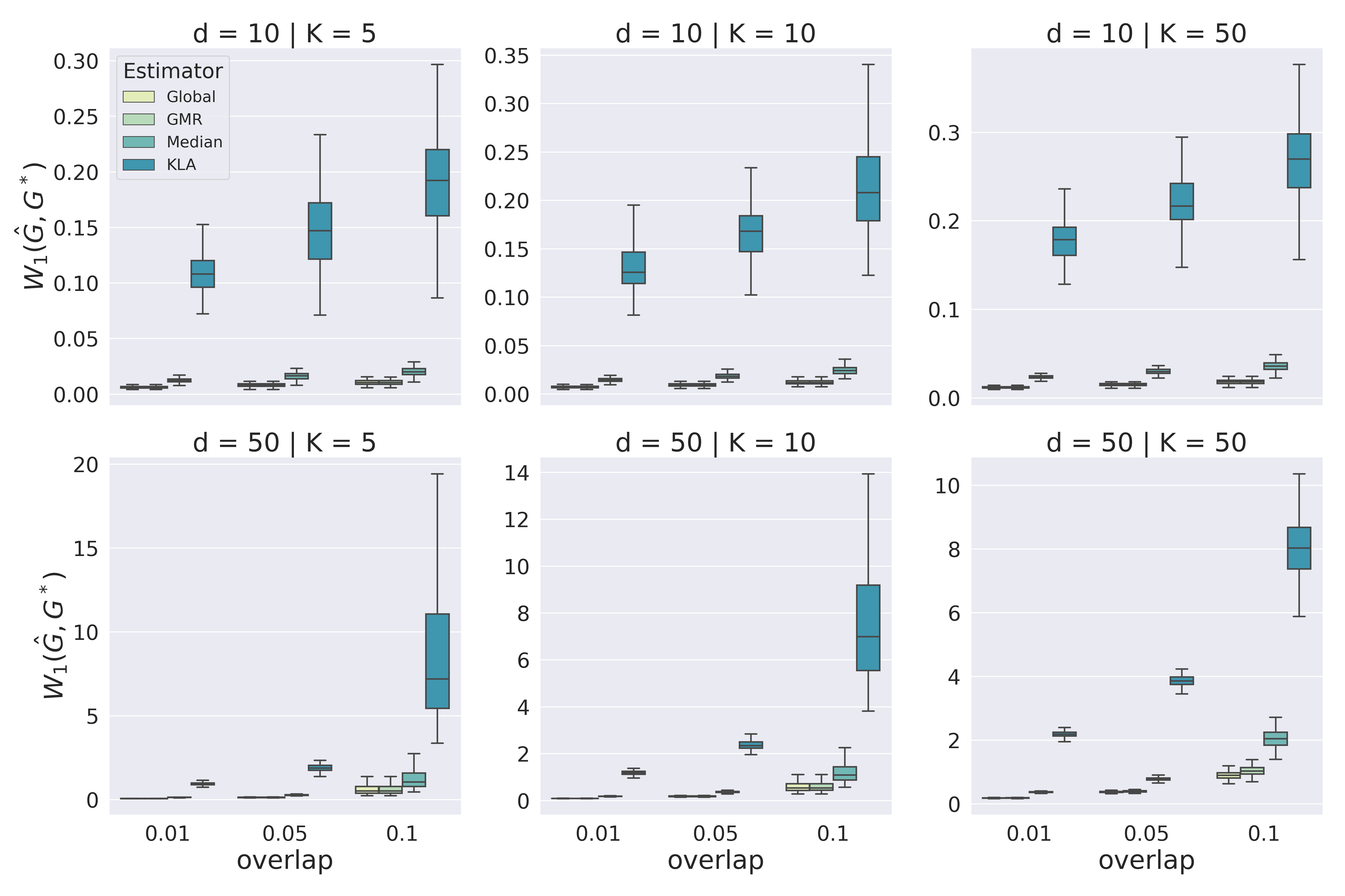
Figure 5: $W_{1}$ distances of estimators for learning mixtures.

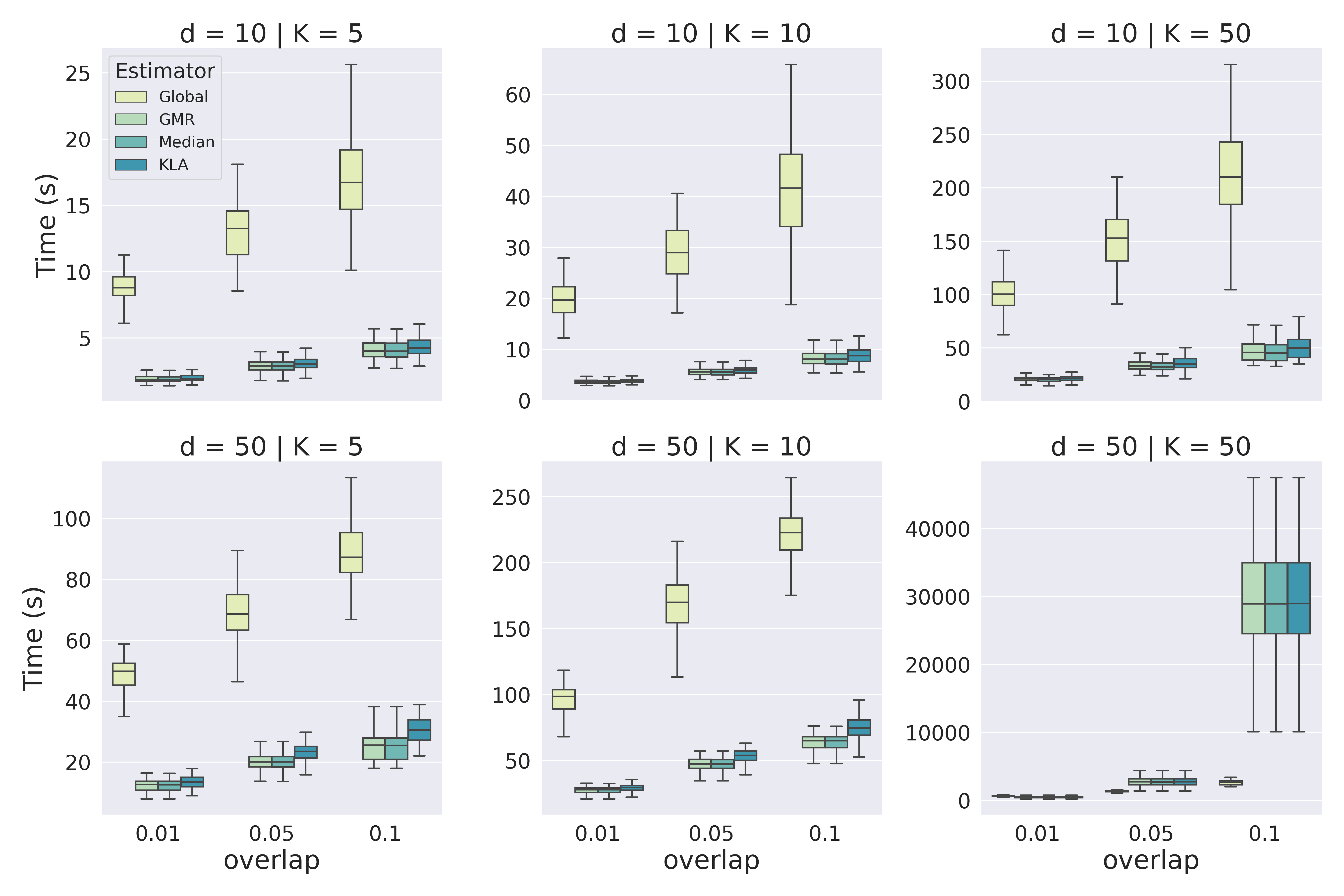
Figure 6: Computational times for learning mixtures.

8.3.2 Convolutional Neural Network in NIST Example

Deep convolutional neural networks (CNNs) are commonly used to reduce the complex structure of a dataset to informative rectangle data. CNNs effectively perform dimension reduction and classification in an end-to-end fashion (Dara and Tumma, 2018). The final soft-max layer in a CNN can be viewed as fitting a multinomial logistic regression model on the reduced feature space. We use a CNN for dimension reduction in the NIST experiment; its architecture is specified in Table 4. We implement the CNN in pytorch 1.5.0 (Paszke et al., 2019) and train it for $10$ epochs on the NIST training dataset. We use the SGD optimizer with learning rate $0.01$, momentum $0.9$, and batch size $64$. After the training, we drop the final layer and use the resulting CNN to reduce to 50 the dimension of the images in the training and test sets.

Table 4: Architecture and layer specifications of CNN for dimension reduction in NIST example.

Layer	Layer specification	Activation function
Conv2d	$C_{\text{in}}=1$, $C_{\text{out}}=20$, $H=W=5$	Relu
MaxPool2d	$k=2$	–
Conv2d	$C_{\text{in}}=20$, $C_{\text{out}}=50$, $H=W=5$	Relu
MaxPool2d	$k=2$	–
Flatten	–	–
Linear	$H_{\text{in}}=800$, $H_{\text{out}}=50$	Relu
Linear	$H_{\text{in}}=50$, $H_{\text{out}}=10$	Softmax

References

- Agrawal et al. (2003) R. Agrawal, A. Evfimievski, and R. Srikant. Information sharing across private databases. In Proceedings of the 2003 ACM SIGMOD International Conference on Management of Data, pages 86–97. ACM, 2003.
- Baldwin (2012) S. Baldwin. Compute canada: advancing computational research. In Journal of Physics: Conference Series, volume 341, page 012001. IOP Publishing, 2012.
- Battey et al. (2015) H. Battey, J. Fan, H. Liu, J. Lu, and Z. Zhu. Distributed estimation and inference with statistical guarantees, 2015. Unpublished manuscript, arXiv:1509.05457.
- Boyd et al. (2011) S. Boyd, N. Parikh, and E. Chu. Distributed optimization and statistical learning via the alternating direction method of multipliers. Now Publishers Inc, 2011.
- Chang et al. (2017) X. Chang, S.-B. Lin, and Y. Wang. Divide and conquer local average regression. Electronic Journal of Statistics, 11(1):1326–1350, 2017.
- Chen (1995) J. Chen. Optimal rate of convergence for finite mixture models. The Annals of Statistics, 23(1):221–233, 1995.
- Chen and Tan (2009) J. Chen and X. Tan. Inference for multivariate normal mixtures. Journal of Multivariate Analysis, 100(7):1367–1383, 2009.
- Chen et al. (2013) W.-C. Chen, G. Ostrouchov, D. Pugmire, Prabhat, and M. Wehner. A parallel EM algorithm for model-based clustering applied to the exploration of large spatio-temporal data. Technometrics, 55(4):513–523, 2013.
- Chen and Xie (2014) X. Chen and M. Xie. A split-and-conquer approach for analysis of extraordinarily large data. Statistica Sinica, 24(4):1655–1684, 2014.
- Corbett et al. (2013) J. C. Corbett, J. Dean, M. Epstein, A. Fikes, C. Frost, J. J. Furman, S. Ghemawat, A. Gubarev, C. Heiser, P. Hochschild, et al. Spanner: Google’s globally distributed database. ACM Transactions on Computer Systems (TOCS), 31(3):Article 8, 2013.
- Cuturi and Doucet (2014) M. Cuturi and A. Doucet. Fast computation of Wasserstein barycenters. In International Conference on Machine Learning, pages 685–693, 2014.
- Dara and Tumma (2018) S. Dara and P. Tumma. Feature extraction by using deep learning: A survey. In 2018 Second International Conference on Electronics, Communication and Aerospace Technology (ICECA), pages 1795–1801. IEEE, 2018.
- Dwivedi et al. (2020) R. Dwivedi, N. Ho, K. Khamaru, M. Wainwright, M. Jordan, and B. Yu. Sharp analysis of expectation-maximization for weakly identifiable models. In International Conference on Artificial Intelligence and Statistics, pages 1866–1876, 2020.
- Fan et al. (2019) J. Fan, D. Wang, K. Wang, and Z. Zhu. Distributed estimation of principal eigenspaces. Annals of Statistics, 47(6):3009–3031, 2019.
- Farnoosh and Zarpak (2008) R. Farnoosh and B. Zarpak. Image segmentation using Gaussian mixture model. IUST International Journal of Engineering Science, 19(1–2):29–32, 2008.
- Feldman et al. (2011) D. Feldman, M. Faulkner, and A. Krause. Scalable training of mixture models via coresets. In Advances in neural information processing systems, pages 2142–2150, 2011.
- Fraley and Raftery (2002) C. Fraley and A. E. Raftery. Model-based clustering, discriminant analysis, and density estimation. Journal of the American Statistical Association, 97(458):611–631, 2002.
- Friedman et al. (2001) J. Friedman, T. Hastie, and R. Tibshirani. The Elements of Statistical Learning, volume 1. Springer Series in Statistics New York, 2001.
- Frühwirth-Schnatter (2006) S. Frühwirth-Schnatter. Finite Mixture and Markov Switching Models. Springer Science & Business Media, 2006.
- Grother and Hanaoka (2016) P. Grother and K. Hanaoka. NIST special database 19 handprinted forms and characters 2nd edition. Technical report, National Institute of Standards and Technology, 2016.
- Heinrich and Kahn (2018) P. Heinrich and J. Kahn. Strong identifiability and optimal minimax rates for finite mixture estimation. The Annals of Statistics, 46(6A):2844–2870, 2018.
- Hunter and Lange (2004) D. R. Hunter and K. Lange. A tutorial on MM algorithms. The American Statistician, 58(1):30–37, 2004.
- Jaggi et al. (2014) M. Jaggi, V. Smith, M. Takac, J. Terhorst, S. Krishnan, T. Hofmann, and M. I. Jordan. Communication-efficient distributed dual coordinate ascent. In Advances in Neural Information Processing Systems 27, pages 3068–3076, 2014.
- Jaini and Poupart (2016) P. Jaini and P. Poupart. Online and distributed learning of Gaussian mixture models by Bayesian moment matching. arXiv preprint arXiv:1609.05881, 2016.
- Jasra et al. (2005) A. Jasra, C. C. Holmes, and D. A. Stephens. Markov chain monte carlo methods and the label switching problem in bayesian mixture modeling. Statistical Science, pages 50–67, 2005.
- Kolouri et al. (2018) S. Kolouri, G. K. Rohde, and H. Hoffmann. Sliced Wasserstein distance for learning Gaussian mixture models. In Proceedings of the IEEE Conference on Computer Vision and Pattern Recognition, pages 3427–3436, 2018.
- Liesenfeld (2001) R. Liesenfeld. A generalized bivariate mixture model for stock price volatility and trading volume. Journal of Econometrics, 104(1):141–178, 2001.
- Liu and Rubin (1994) C. Liu and D. B. Rubin. The ECME algorithm: A simple extension of EM and ECM with faster monotone convergence. Biometrika, 81(4):633–648, 1994.
- Liu and Ihler (2014) Q. Liu and A. T. Ihler. Distributed estimation, information loss and exponential families. In Advances in Neural Information Processing Systems 27, pages 1098–1106, 2014.
- Lucic et al. (2017) M. Lucic, M. Faulkner, A. Krause, and D. Feldman. Training gaussian mixture models at scale via coresets. The Journal of Machine Learning Research, 18(1):5885–5909, 2017.
- Maitra and Melnykov (2010) R. Maitra and V. Melnykov. Simulating data to study performance of finite mixture modeling and clustering algorithms. Journal of Computational and Graphical Statistics, 19(2):354–376, 2010.
- McLachlan and Peel (2004) G. McLachlan and D. Peel. Finite Mixture Models. John Wiley & Sons, 2004.
- Meilijson (1989) I. Meilijson. A fast improvement to the EM algorithm on its own terms. Journal of the Royal Statistical Society: Series B (Methodological), 51(1):127–138, 1989.
- Melnykov et al. (2012) V. Melnykov, W.-C. Chen, and R. Maitra. MixSim: An R package for simulating data to study performance of clustering algorithms. Journal of Statistical Software, 51(12):1–25, 2012.
- Meng and Rubin (1993) X.-L. Meng and D. B. Rubin. Maximum likelihood estimation via the ECM algorithm: A general framework. Biometrika, 80(2):267–278, 1993.
- Murphy (2012) K. P. Murphy. Machine learning: a probabilistic perspective. MIT press, 2012.
- Neal and Hinton (1998) R. M. Neal and G. E. Hinton. A view of the EM algorithm that justifies incremental, sparse, and other variants. In Learning in Graphical Models, pages 355–368. Springer, 1998.
- Nguyen (2013) X. Nguyen. Convergence of latent mixing measures in finite and infinite mixture models. The Annals of Statistics, 41(1):370–400, 2013.
- Nowak (2003) R. D. Nowak. Distributed EM algorithms for density estimation and clustering in sensor networks. IEEE Transactions on Signal Processing, 51(8):2245–2253, 2003.
- Paszke et al. (2019) A. Paszke, S. Gross, F. Massa, A. Lerer, J. Bradbury, G. Chanan, T. Killeen, Z. Lin, N. Gimelshein, L. Antiga, A. Desmaison, A. Kopf, E. Yang, Z. DeVito, M. Raison, A. Tejani, S. Chilamkurthy, B. Steiner, L. Fang, J. Bai, and S. Chintala. Pytorch: An imperative style, high-performance deep learning library. In Advances in Neural Information Processing Systems 32, pages 8026–8037, 2019.
- Pearson (1894) K. Pearson. Contributions to the mathematical theory of evolution. Philosophical Transactions of the Royal Society of London. A, 185:71–110, 1894.
- Pedregosa et al. (2011) F. Pedregosa, G. Varoquaux, A. Gramfort, V. Michel, B. Thirion, O. Grisel, M. Blondel, P. Prettenhofer, R. Weiss, V. Dubourg, J. Vanderplas, A. Passos, D. Cournapeau, M. Brucher, M. Perrot, and E. Duchesnay. Scikit-learn: Machine learning in Python. Journal of Machine Learning Research, 12:2825–2830, 2011.
- Peyré and Cuturi (2019) G. Peyré and M. Cuturi. Computational optimal transport: With applications to data science. Foundations and Trends® in Machine Learning, 11(5–6):355–607, 2019.
- Plataniotis and Hatzinak (2000) K. N. Plataniotis and D. Hatzinak. Gaussian mixtures and their applications to signal processing. In S. Stergiopoulos, editor, Advanced Signal Processing Handbook: Theory and Implementation for Radar, Sonar, and Medical Imaging Real Time Systems, volume 25, chapter 3, pages 3-1–3-35. CRC Press, Boca Raton, 1 edition, 2000.
- Rousseau and Mengersen (2011) J. Rousseau and K. Mengersen. Asymptotic behaviour of the posterior distribution in overfitted mixture models. Journal of the Royal Statistical Society: Series B (Methodological), 73(5):689–710, 2011.
- Safarinejadian et al. (2010) B. Safarinejadian, M. B. Menhaj, and M. Karrari. A distributed EM algorithm to estimate the parameters of a finite mixture of components. Knowledge and Information Systems, 23(3):267–292, 2010.
- Santosh et al. (2013) D. H. H. Santosh, P. Venkatesh, P. Poornesh, L. N. Rao, and N. A. Kumar. Tracking multiple moving objects using Gaussian mixture model. International Journal of Soft Computing and Engineering (IJSCE), 3(2):114–119, 2013.
- Schieferdecker and Huber (2009) D. Schieferdecker and M. F. Huber. Gaussian mixture reduction via clustering. In 2009 12th International Conference on Information Fusion, pages 1536–1543. IEEE, 2009.
- Van der Vaart (2000) A. W. Van der Vaart. Asymptotic Statistics, volume 3. Cambridge University Press, 2000.
- Villani (2003) C. Villani. Topics in Optimal Transportation, volume 58. American Mathematical Society, 2003.
- Williams and Maybeck (2006) J. L. Williams and P. S. Maybeck. Cost-function-based hypothesis control techniques for multiple hypothesis tracking. Mathematical and Computer Modelling, 43(9–10):976–989, 2006.
- Wu (1983) C. J. Wu. On the convergence properties of the EM algorithm. The Annals of Statistics, 11(1):95–103, 1983.
- Yu et al. (2018) L. Yu, T. Yang, and A. B. Chan. Density-preserving hierarchical EM algorithm: Simplifying Gaussian mixture models for approximate inference. IEEE Transactions on Pattern Analysis and Machine Intelligence, 41(6):1323–1337, 2018.
- Zangwill (1969) W. I. Zangwill. Nonlinear Programming: A Unified Approach, volume 52. Prentice-Hall Englewood Cliffs, NJ, 1969.
- Zhang and Chen (2020) Q. Zhang and J. Chen. A unified framework for gaussian mixture reduction with composite transportation distance. arXiv preprint arXiv:2002.08410, 2020.
- Zhang et al. (2015) Y. Zhang, J. Duchi, and M. Wainwright. Divide and conquer kernel ridge regression: A distributed algorithm with minimax optimal rates. The Journal of Machine Learning Research, 16(1):3299–3340, 2015.