Variational Dynamic Mixtures

Abstract

Deep probabilistic time series forecasting models have become an integral part of machine learning. While several powerful generative models have been proposed, we provide evidence that their associated inference models are oftentimes too limited and cause the generative model to predict mode-averaged dynamics. Mode-averaging is problematic since many real-world sequences are highly multi-modal, and their averaged dynamics are unphysical (e.g., predicted taxi trajectories might run through buildings on the street map). To better capture multi-modality, we develop variational dynamic mixtures (VDM): a new variational family to infer sequential latent variables. The VDM approximate posterior at each time step is a mixture density network, whose parameters come from propagating multiple samples through a recurrent architecture. This results in an expressive multi-modal posterior approximation. In an empirical study, we show that VDM outperforms competing approaches on highly multi-modal datasets from different domains.

1 Introduction

Making sense of time series data is an important challenge in various domains, including ML for climate change. One important milestone to reach the climate goals is to significantly reduce the $\text{CO}_{2}$ emissions from mobility (rogelj2016paris). Accurate forecasting models of typical driving behavior and of typical pollution levels over time can help both lawmakers and automotive engineers to develop solutions for cleaner mobility. In these applications, no accurate physical model of the entire dynamic system is known or available. Instead, data-driven models, specifically deep probabilistic time series models, can be used to solve the necessary tasks including forecasting.

The dynamics in such data can be highly multi-modal. At any given part of the observed sequence, there might be multiple distinct continuations of the data that are plausible, but the average of these behaviors is unlikely, or even physically impossible. Consider for example a dataset of taxi trajectories. In each row of Fig. 1(a), we have selected 50 routes from the dataset with similar starting behavior (blue). Even though these routes are quite similar to each other in the first 10 way points, the continuations of the trajectories (red) can exhibit quite distinct behaviors and lead to points on any far edge of the map. The trajectories follow a few main traffic arteries, these could be considered the main modes of the data distribution. We would like to learn a generative model of the data, that based on some initial way points, can forecast plausible continuations for the trajectories.

Many existing methods make restricting modeling assumptions such as Gaussianity to make learning tractable and efficient. But trying to capture the dynamics through unimodal distributions can lead either to “over-generalization”, (i.e. putting probability mass in spurious regions) or on focusing only on the dominant mode and thereby neglecting important structure of the data. Even neural approaches, with very flexible generative models can fail to fully capture this multi-modality because their capacity is often limited through the assumptions of their inference model. To address this, we develop variational dynamic mixtures (VDM). Its generative process is a sequential latent variable model. The main novelty is a new multi-modal variational family which makes learning and inference multi-modal yet tractable. In summary, our contributions are

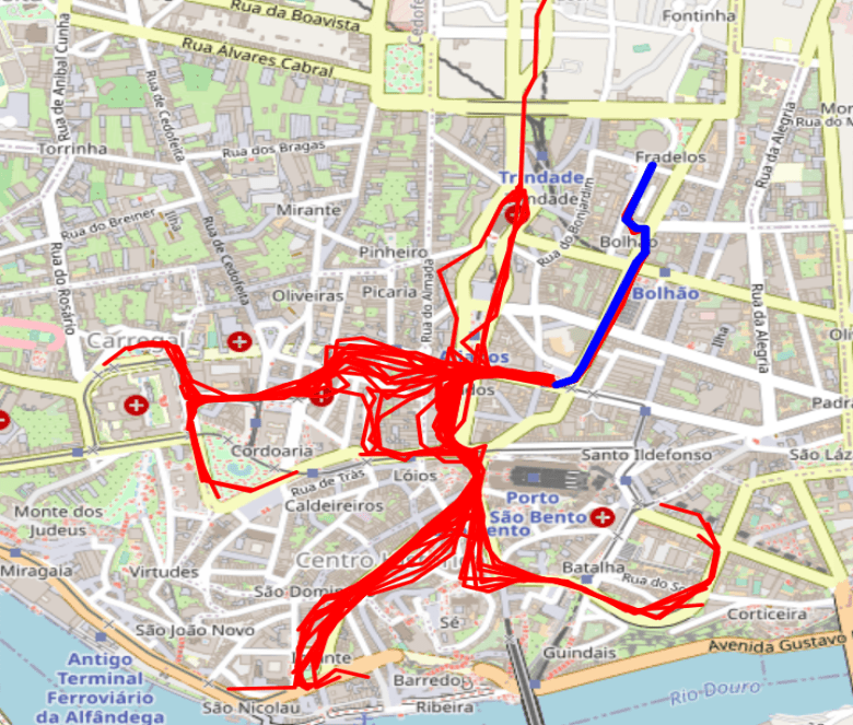
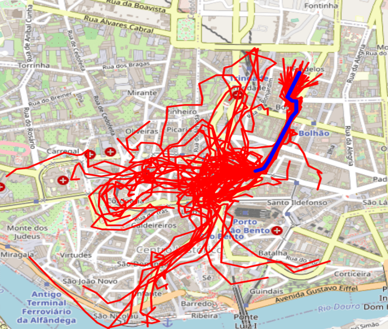
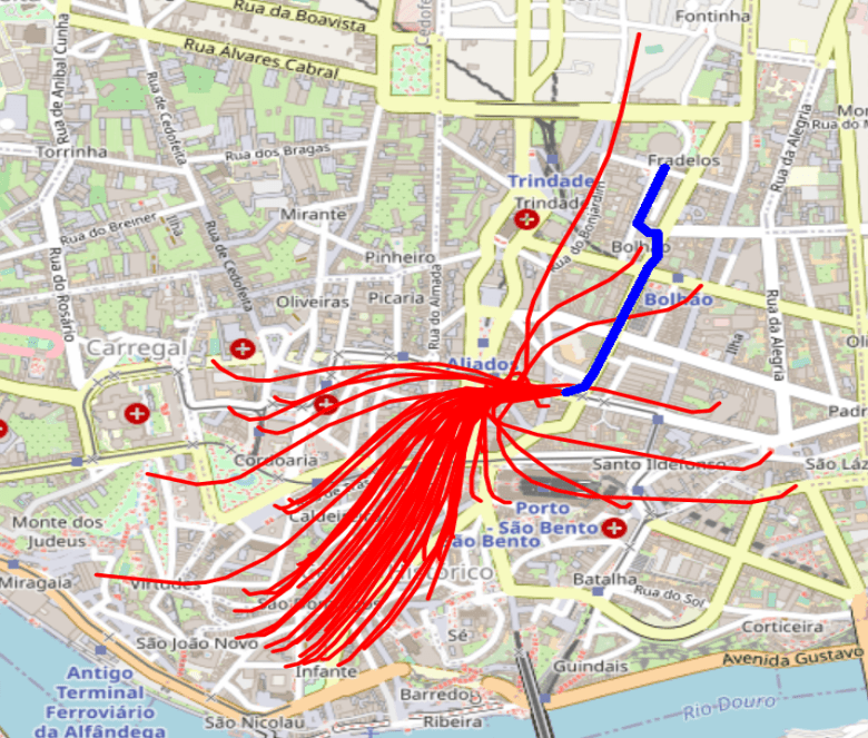
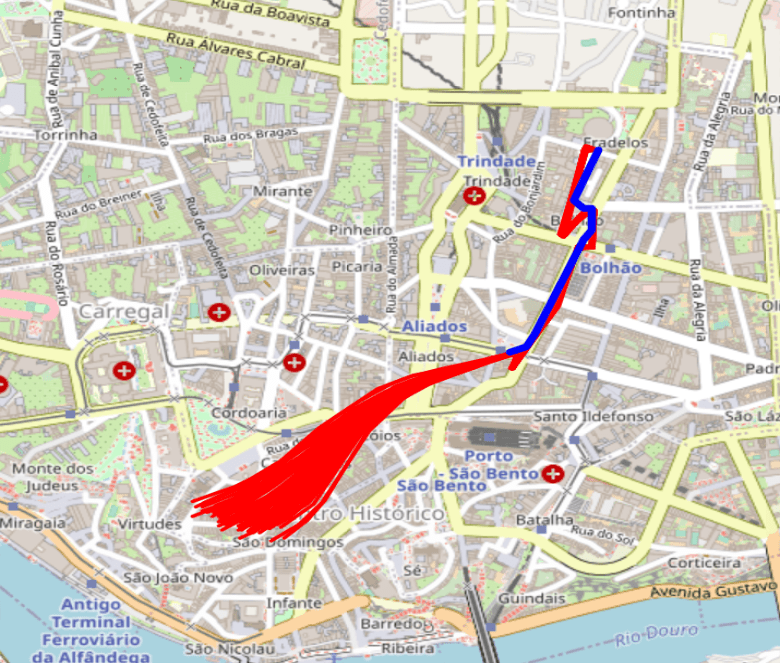
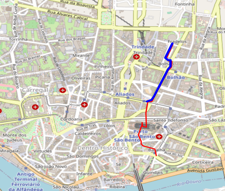
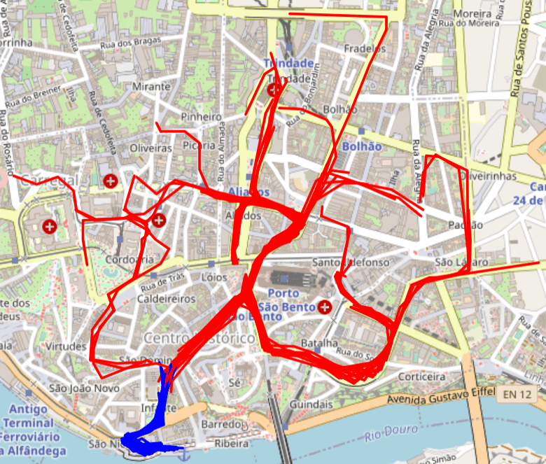
(a) Taxi Data

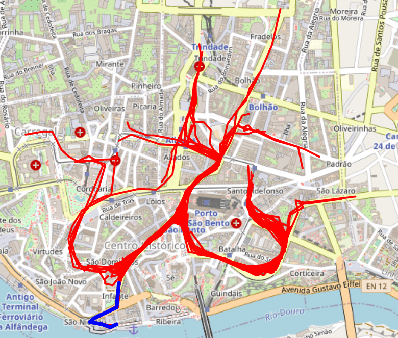
(b) VDM (ours)

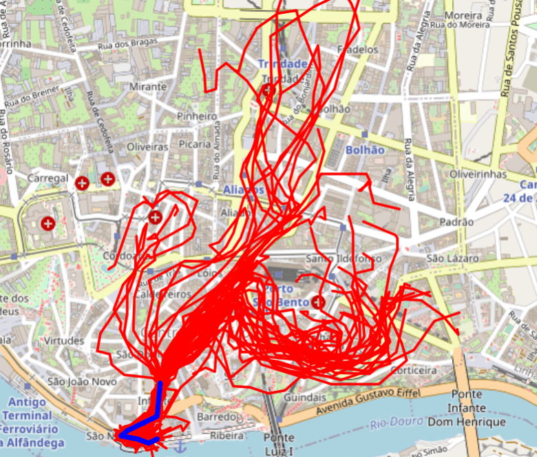
(c) AESMC

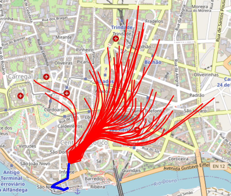
(d) CF-VAE

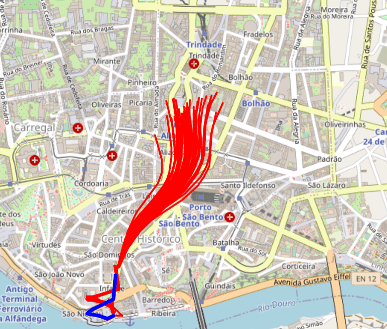
(e) VRNN

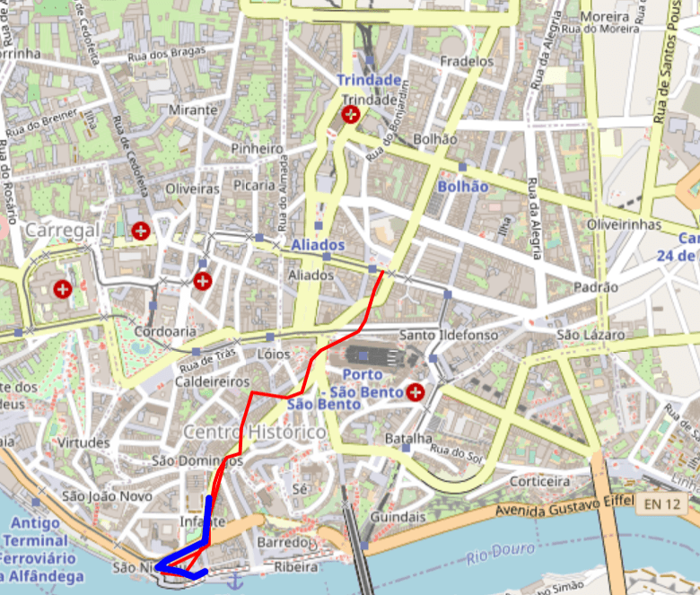
(f) RKN

Figure 1: Forecasting taxi trajectories is challenging due to the highly multi-modal nature of the data (Fig. 1(a)). VDM (Fig. 1(b)) succeeds in generating diverse plausible predictions (red), based the beginning of a trajectory (blue). The other methods, AESMC (le2018auto), CF-VAE (bhattacharyya2019conditional), VRNN chung2015recurrent, RKN becker2019recurrent, suffer from mode averaging.

• A new inference model. We establish a new type of variational family for variational inference of sequential latent variables. By successively marginalizing over previous latent states, the procedure can be efficiently carried-out in a single forward pass and induces a multi-modal posterior approximation. We can see in Fig. 1(b), that VDM trained on a dataset of taxi trajectories produces forecasts with the desired multi-modality while other methods overgeneralize.

• An evaluation metric for multi-modal tasks. The negative log-likelihood measures predictive accuracy but neglects an important aspect of multi-modal forecasts – sample diversity. In LABEL:sec:exp, we derive a score based on the Wasserstein distance (villani2008optimal) which evaluates both sample quality and diversity. This metric complements our evaluation based on log-likelihoods.

• An extensive empirical study. in LABEL:sec:exp, we use VDM to study various datasets, including a synthetic data with four modes, a stochastic Lorenz attractor, the taxi trajectories, and a U.S. pollution dataset with the measurements of various pollutants over time. We illustrate VDM’s ability in modeling multi-modal dynamics, and provide quantitative comparisons to other methods showing that VDM compares favorably to previous work.

2 Related Work

Neural recurrent models.

Recurrent neural networks (RNNs) such as LSTMs (hochreiter1997long) and GRUs (chung2014empirical) have proven successful on many time series modeling tasks. However, as deterministic models they cannot capture uncertainties in their dynamic predictions. Stochastic RNNs make these sequence models non-deterministic (chung2015recurrent; fraccaro2016sequential; gemici2017generative; li2018disentangled). For example, the variational recurrent neural network (VRNN) (chung2015recurrent) enables multiple stochastic forecasts due to its stochastic transition dynamics. An extension of VRNN (goyal2017z) uses an auxiliary cost to alleviate the KL-vanishing problem. It improves on VRNN inference by forcing the latent variables to also be predictive of future observations. Another line of related methods rely on particle filtering (naesseth2018variational; le2018auto; hirt2019scalable) and in particular sequential Monte Carlo (SMC) to improve the evidence lower bound. In contrast, VDM adopts an explicitly multi-modal posterior approximation. Another SMC-based work (saeedi2017variational) employs search-based techniques for multi-modality but is limited to models with finite discrete states. Recent works (schmidt2018deep; schmidt2019autoregressive; ziegler2019latent) use normalizing flows in the latent space to model the transition dynamics. A normalizing flow requires many layers to transform its base distribution into a truly multi-modal distribution in practice. In contrast, mixture density networks (as used by VDM) achieve multi-modality by mixing only one layer of neural networks. A task orthogonal to multi-modal inference is learning disentangled representations. Here too, mixture models are used (chen2016infogan; li2017infogail). These papers use discrete variables and a mutual information based term to disentangle different aspects of the data.

VAE-like models (bhattacharyya2018accurate; bhattacharyya2019conditional) and GAN-like models (sadeghian2019sophie; kosaraju2019social) only have global, time independent latent variables. Yet, they show good results on various tasks, including forecasting. With a deterministic decoder, these models focus on average dynamics and don’t capture local details (including multi-modal transitions) very well. Sequential latent variable models are described next.

Deep state-space models.

Classical state-space models (SSMs) are popular due to their tractable inference and interpretable predictions. Similarly, deep SSMs with locally linear transition dynamics enjoy tractable inference (karl2016deep; fraccaro2017disentangled; rangapuram2018deep; becker2019recurrent). However, these models are often not expressive enough to capture complex (or highly multi-modal) dynamics. Nonlinear deep SSMs (krishnan2017structured; zheng2017state; doerr2018probabilistic; de2019gru; gedon2020deep) are more flexible. Their inference is often no longer tractable and requires variational approximations. Unfortunately, in order for the inference model to be tractable, the variational approximations are often simplistic and don’t approximate multi-modal posteriors well with negative effects on the trained models. Multi-modality can be incorporated via additional discrete switching latent variables, such as recurrent switching linear dynamical systems (linderman2017bayesian; nassar2018tree; becker2019switching). However, these discrete states make inference more involved.

3 Variational Dynamic Mixtures

We develop VDM, a new sequential latent variable model for multi-modal dynamics. Given sequential observations $\mathbf{x}_{1:T}=(\mathbf{x}_{1},\ldots,\mathbf{x}_{T})$, VDM assumes that the underlying dynamics are governed by latent states $\mathbf{z}_{1:T}=(\mathbf{z}_{1},\ldots,\mathbf{z}_{T})$. We first present the generative process and the multi-modal inference model of VDM. We then derive a new variational objective that encourages multi-modal posterior approximations and we explain how it is regularized via hybrid-training. Finally, we introduce a new sampling method used in the inference procedure.

Generative model.

The generative process consists of a transition model and an emission model. The transition model $p(\mathbf{z}_{t}\mid\mathbf{z}_{<t})$ describes the temporal evolution of the latent states and the emission model $p(\mathbf{x}_{t}\mid\mathbf{z}_{\leq t})$ maps the states to observations. We assume they are parameterized by two separate neural networks, the transition network $\phi^{tra}$ and the emission network $\phi^{dec}$. To give the model the capacity to capture longer range temporal correlations we parametrize the transition model with a recurrent architecture $\phi^{\text{GRU}}$ (auger2016state; zheng2017state) such as a GRU (chung2014empirical). The latent states $\mathbf{z}_{t}$ are sampled recursively from

$$\mathbf{z}_{t}\mid\mathbf{z}_{<t}\sim\mathcal{N}(\mathbf{\mu}_{0,t},\mathbf{\sigma}_{0,t}^{2}\mathbb{I}),\quad\text{where}\quad[\mathbf{\mu}_{0,t},\mathbf{\sigma}_{0,t}^{2}]=\phi^{tra}(\mathbf{h}_{t-1}),\,\mathbf{h}_{t-1}=\phi^{\text{GRU}}(\mathbf{z}_{t-1},\mathbf{h}_{t-2}),$$ (1)

and are then decoded such that the observations can be sampled from the emission model,

$$\mathbf{x}_{t}\mid\mathbf{z}_{\leq t}\sim\mathcal{N}(\mathbf{\mu}_{x,t},\mathbf{\sigma}_{x,t}^{2}\mathbb{I}),\quad\text{where}\quad[\mathbf{\mu}_{x,t},\mathbf{\sigma}_{x,t}^{2}]=\phi^{dec}(\mathbf{z}_{t},\mathbf{h}_{t-1}).$$ (2)

This generative process is similar to (chung2015recurrent), though we did not incorporate autoregressive feedback due to its negative impact on long-term generation (ranzato2015sequence; lamb2016professor). The competitive advantage of VDM comes from a more expressive inference model.

Inference model.

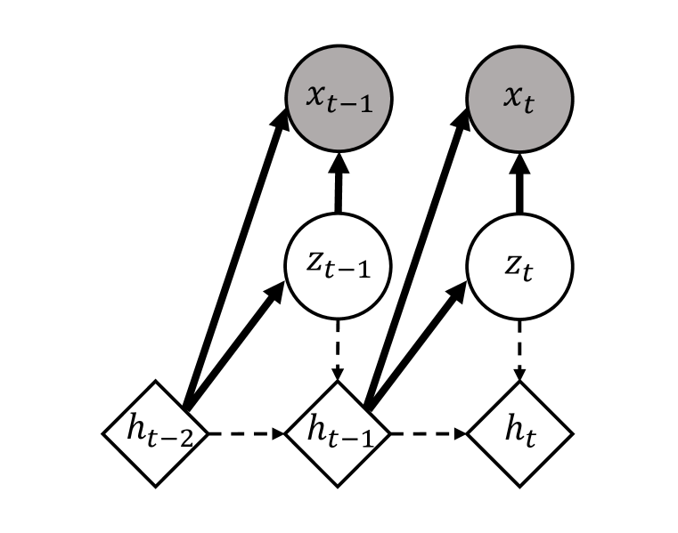
(a) Generation (Eqs. 1 and 2)

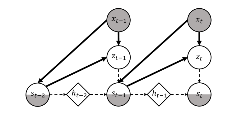
(b) Inference (LABEL:eqn:qtilde, LABEL:eqn:inference and LABEL:eqn:expected_h)

Figure 2: Graphical illustrations of VDM. Dashed lines denote deterministic dependencies such as transformations, marginalization, or computing the mean, as explained in the main text, while bold lines denote stochastic dependencies. The half-shaded node for $\mathbf{s}_{t}$ indicates that $\mathbf{s}_{t}$ is being marginalized out as opposed to conditioned on.

VDM is based on a new procedure for multi-modal inference. The main idea is that to approximate the posterior at time $t$, we can use the posterior approximation of the previous time step and exploit the generative model’s transition model $\phi^{\text{GRU}}$. This leads to a sequential inference procedure. We first use the forward model to transform the approximate posterior at time $t-1$ into a distribution at time $t$. In a second step, we use samples from the resulting transformed distribution and combine each sample with data evidence $\mathbf{x}_{t}$, where every sample parameterizes a Gaussian mixture component. As a result, we obtain a multi-modal posterior distribution that depends on data evidence, but also on the previous time step’s posterior.

In more detail, for every $\mathbf{z}_{t}$, we define its corresponding recurrent state as the transformed random variable $\mathbf{s}_{t}=\phi^{\text{GRU}}(\mathbf{z}_{t},\mathbf{h}_{t-1})$, using a deterministic hidden state $\mathbf{h}_{t-1}=\mathbb{E}\left[\mathbf{s}_{t-1}\right]$. The variational family of VDM is defined as follows:

$$q(\mathbf{z}_{1:T}\mid\mathbf{x}_{1:T})=\prod_{t=1}^{T}q(\mathbf{z}_{t}\mid\mathbf{x}_{\leq t})=\prod_{t=1}^{T}\int q(\mathbf{z}_{t}\mid\mathbf{s}_{t-1},\mathbf{x}_{t})q(\mathbf{s}_{t-1}\mid\mathbf{x}_{\leq t})\mathrm{d}\mathbf{s}_{t-1}.$$ (3)

chung2015recurrent also use a sequential inference procedure, but without considering the distribution of $\mathbf{s}_{t}$. Only a single sample is propagated through the recurrent network and all other information about the distribution of previous latent states $\mathbf{z}_{<t}$ is lost. In contrast, VDM explicitly maintains $\mathbf{s}_{t}$ as part of the inference model. Through marginalization, the entire distribution is taken into account for inferring the next state $\mathbf{z}_{t}$. Beyond the factorization assumption and the marginal consistency constraint of Eq. 3, the variational family of VDM needs two more choices to be fully specified; First, one has to choose the parametrizations of $q(\mathbf{z}_{t}\mid\mathbf{s}_{t-1},\mathbf{x}_{t})$ and $q(\mathbf{s}_{t-1}\mid\mathbf{x}_{\leq t})$ and second, one has to choose a sampling method to approximate the marginalization in Eq. 3. These choices determine the resulting factors $q(\mathbf{z}_{t}\mid\mathbf{x}_{\leq t})$ of the variational family.

We assume that the variational distribution of the recurrent state factorizes as $q(\mathbf{s}_{t-1}\mid\mathbf{x}_{\leq t})=\omega(\mathbf{s}_{t-1},\mathbf{x}_{t})\tilde{q}(\mathbf{s}_{t-1}\mid\mathbf{x}_{<t})$, i.e. it is the distribution of the recurrent state given the past observation, re-weighted by a weighting function $\omega(\mathbf{s}_{t-1},\mathbf{x}_{t})$ which involves only the current observations. For