End-to-end Wireless Path Deployment with Intelligent Surfaces Using Interpretable Neural Networks

Abstract

Intelligent surfaces exert deterministic control over the wireless propagation phenomenon, enabling novel capabilities in performance, security and wireless power transfer. Such surfaces come in the form of rectangular tiles that cascade to cover large surfaces such as walls, ceilings or building facades. Each tile is addressable and can receive software commands from a controller, manipulating an impinging electromagnetic wave upon it by customizing its reflection direction, focus, polarization and phase. A new problem arises concerning the orchestration of a set of tiles towards serving end-to-end communication objectives. Towards that end, we propose a novel intelligent surface networking algorithm based on interpretable neural networks. Tiles are mapped to neural network nodes and any tile line-of-sight connectivity is expressed as a neural network link. Tile wave manipulation functionalities are captured via geometric reflection with virtually rotatable tile surface norm, thus being able to tunable distribute power impinging upon a tile over the corresponding neural network links, with the corresponding power parts acting as the link weights. A feedforward/backpropagate process optimizes these weights to match ideal propagation outcomes (normalized network power outputs) to wireless user emissions (normalized network power inputs). An interpretation process translates these weights to the corresponding tile wave manipulation functionalities.

I Introduction

In recent years, the development of wireless communication technologies has undergone an unprecedented growth with the proliferation of smart wireless devices and burgeons of the Internet of Things (IoT). The goals to achieve higher throughput, lower latency, better services, and lower prices have driven the research efforts into the fifth and sixth-generation mobile networks, narrow-band IoT, new generation WLANs IEEE802.11ax/ay, among other promising techniques to overcome the challenges of limited spectrum resources and higher user densities [1, 2, 3]. Most of the currently proposed solutions in the physical layer focus on the improvement of transceiver design, for instance, the massive MIMO communication system equips base stations with more than one hundred antennas to improve the spatial diversity and overall antenna gain. Nonetheless, techniques on mere transceiver advancements do not overcome system limitations, and they also suffer from intrinsic design issues (e.g., self-interference from duplex communications, channel aging in precoding, and so on). Hence, non-conventional solutions should be sought.

One important yet largely overlooked factor is the wireless propagation environment itself, which directly influences the performance of wireless links. In regular wireless propagation environments, the radiated electromagnetic (EM) waves experience various effects, including reflection, diffraction, scattering, penetration, among others, which create rich multi-path conditions. Such multi-path propagation, if not well-controlled, could cause destructive interference at the user-ends. Additionally, energy dissipation occurs with such propagation effects, thus limiting the received signal strength. In order to minimize such adversarial effects and preserve energy along transmission, the propagation environments need to be controlled strategically. With the use of novel materials, the propagation environments can be transformed into programmable media, yielding unparalleled, wired-level gains in wireless power transfer, and mitigate interference, Doppler effects, as well as malicious eavesdropping [4, 5, 6]. In order to perform an adaptive control over the programmable wireless propagation channel, a novel solution based on artificial materials has been conceived, utilizing software-defined metasurfaces (SDMs) [7, 8].

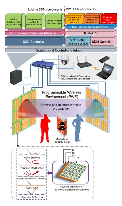
Figure 1: Schematic displaying the inter-networking of SDMs and their end-to-end workflow, enabling operation modes in a programmable wireless environment (PWE), illustrated with a pair of a transmitter and a receiver. The layers of an SDM unit (tile) include (a) the metasurface, (b) the sensing and actuation, (c) the computing, and (d) the gateway/communications planes.

The SDMs, when embedded within a physical setting, result into a Programmable Wireless Environment (PWE) wherein wireless propagation can be even completely customized [5]. SDMs empower PWEs by achieving the following functionalities (Fig. 1): 1) Controlling the propagation direction of the signal. For example, when EM waves impinge on a flat surface, the law of specular reflection dictates the direction of reflection. However, the SDMs can steer the reflected EM waves towards alternate directions, such that useful signals can be directed towards the destined user, while interference can be mitigated; 2) Tuning the phase of the signal. Specifically, during a coherent combining at the receiver side with multi-paths, signals could be totally canceled out due to a $180^{\circ}$ phase difference. With the phase-tuning capability of SDMs, the signal level will be strengthened upon reception; 3) Modifying the polarization of the signal. While some radiated signals are linearly polarized, interactions with surrounding environments can alter their polarization. The polarization mismatch will also cause degradation in link performance. The SDMs can perform polarization tuning so that the signals are robust against such distortion.

In this paper, we propose a solution for the networking of sets of SDM units–denoted as tiles–which are deployed within an environment, e.g. over indoor walls or building facade. The problem is to define the exact EM wave manipulation type that each tile should exert (e.g., steer a wave toward a custom direction), in order to optimally serve a set of communicating user objectives (e.g., maximizing the received power). The key idea is that, since SDM tiles can regulate the distribution of power within a space, they can be represented by nodes in a neural network, while the wireless propagation paths can be mapped to neural network links and their weights. The neural network is optimized via a custom feed-forward/back-propagation process, and its elements are interpreted into SDM tile functionalities. The machine learning approach is shown to be intuitive in its representation, operate collaboratively with existing techniques and be economic in its use of SDM tiles, compared to related approaches [5]. The contributions are:

• We propose a novel approach that constitutes common feedforward/backpropagation-based neural networks applicable to the optimization of PWEs. Using the proposed approach, the structure and training state of neural networks becomes directly interpretable to the floorplan geometry and the configuration of its contained SDM tiles.

• Subsequently, we propose a specific scheme for optimizing PWEs, named NNConfig; We map the trained neural networks to tile configurations in order to achieve EM wave control functionalities, including wave steering, absorption, and wave splitting.

• We demonstrate through extensive simulations that such interpretable neural networks can deduce PWE configurations that surpass existing approaches, by detecting complex solutions where a single tile serves multiple purposes. Subsequently, the number of tiles required to serve a pair of wireless devices is reduced, benefiting PWE scalability, capacity and cost.

The remainder of this is work is as follows. Section II surveys the related studies and provide the necessary prerequisites on networking intelligent surfaces. Section III presents the novel scheme and its evaluation via simulations takes place in Section IV. The paper is concluded in Section V.

II Related Work

Presently, the related literature moves into two disjoint directions, summarized in Fig. 2:

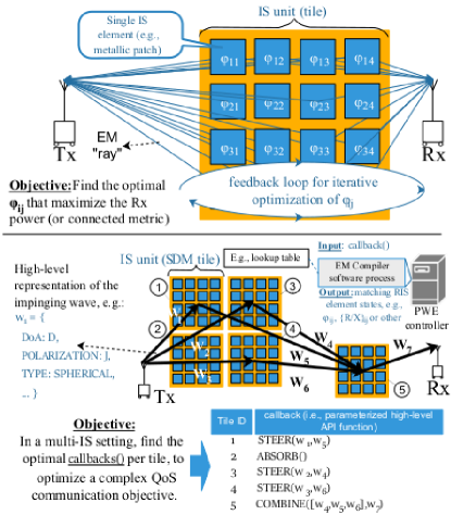
Figure 2: Separation of concerns in the literature. (Top): deducing the optimal meta-atom phases (and sometime amplitudes) to yield a high level intelligent surface functionality (e.g., steering). (Bottom): In a multi-surface deployment, deduce the optimal parameterized high-level functionalities per surface tile, to serve the user communication objectives.

We will denote the first direction, shown at the top, as the Intelligent Surface (IS) Physical-Layer. This direction commonly assumes a single IS and a set of RX-TX. The IS is configured via the phased antenna array analytical model, meaning that each tile is treated as an antenna array with individually controlled re-radiation phase $\phi_{ij}$ (and in some case, re-radiation amplitude $a_{ij}$ as well) [9]. The objective of this line of work is to deduce the optimal $\phi_{ij}$ values that optimize the received EM wave, e.g., its power in the simplest case, and extending to channel quality control in general [10, 11, 12], (albeit bearing different names, such as “large intelligent surfaces”, “intelligent reconfigurable surfaces”, “holographic MIMO surfaces”, among others [13, 14, 15, 16, 17, 18, 19, 20, 21]). This is accomplished by establishing a feedback loop between the RX and the TX, and applying an iterative optimization process, including innovative neural networks accelerators that speed up the optimization process [22, 23]. Other studies close to this direction seek to optimize the geometry and material composition of the IS for optimal operation in a given band or application setting [24] (e.g., WiFi). We remark that a vast number of designs, comprising diverse materials and manufacturing approaches, has been proposed in the literature over the past 20 years [25, 20], and the reader is directed to a recent survey on this topic [26].

The second direction, shown at the lower part of Fig. 2, will be denoted as IS Network-Layer. This direction assumes a system architecture based on the SDM paradigm, i.e., networked ISs which are centrally controlled by a server (PWE controller) [5, 27, 28, 4, 29]. Multiple SDM units are placed within an environment, with the utter goal of ideally exerting complete control over the wireless propagation phenomenon within a space (i.e., a PWE). SDMs decouple the functionality-level multi-IS orchestration logic from the underlying IS Physical-layer as follows:

• The EM waves are modeled at a high-level as data structures, with an example shown in Fig. 2. Similarly, the possible/supported EM wave manipulations by a SDM are modeled as software callbacks, as shown in both Fig. 1 and Fig. 2. These data structures and callbacks are collectively denoted as the SDM Application programming Interface (API)  [30].

• A software middleware residing inside the PWE controller, denoted as the EM Compiler  [31], translates callbacks to matching meta-atom states per tile, such as phases $\phi_{ij}$, or even directly to local surface impedance values R/X, when a specific IS Physical-Layer design/material is considered [32]. The works in the IS Physical-Layer direction could fill the role of the EM Compiler. However, to support real-time operation, SDMs use a lookup table containing all supported functionalities. This table is populated during the SDM manufacturing, using real field measurements. A report on the experimental verification of this process can be found online [33]. A mechanism for interleaving multiple high-level functionalities (callbacks) over the same tile on-the-fly is also supported. In this manner, real-time operation is facilitated, while the PWE control logic as a whole is decoupled from the multitude of RIS physical design variations, thus becoming a reusable control module.

Based on this categorization, the present work falls into the IS Network-Layer direction, and its objective is to define the optimal high-level functionality (or callback) for each tile within a PWE, to meet a QoS objective for the communicating user pairs, as exemplary shown in Fig. 1-2.

Based on the discussion above, it is clarified that the IS Physical-Layer and IS Network-Layer literature directions have different objectives, which make them complimentary in their nature, and not otherwisely comparable.

II-A Prerequisites: Networking Metasurfaces

As shown in Fig. 1, via their gateways, the SDMs within a PWE are networked [34], i.e., become centrally monitored and configured via a server, in order to serve a particular end-objective. Specifically, a set of SDMs is configured with appropriate EM wave steering and focusing commands to route EM waves exchanged between a pair of wireless users in an unnatural manner, avoiding obstacles or eavesdroppers [5]. Other examples include wireless power transfer and wireless channel customization for advanced QoS [35, 34]. Using a software-defined networking (SDN)-compatible architecture [36], a PWE can inter-operate with existing SDN applications [5]. For instance, a device localization application can inform the PWE controller of the approximate user device locations within a space [37, 38, 39]. A user access SDN application can further deduce the access level that each device should have. Subsequently, the PWE can tune the SDM tiles to avoid, e.g., potentially malevolent users.

PWEs have the potential to provide full, software-defined control over the wireless propagation phenomenon. This can yield groundbreaking capabilities such as [13, 14, 15, 16, 17, 18, 19, 20, 21, 5, 28]: i) Extremely efficient mitigation of path loss and multi-path fading phenomena, allowing not only for more efficient communications, but also for long-range wireless power transfer. ii) Cross-device interference cancellation and wireless channel capacity maximization. iii) Physical-layer security via: SINR minimization around unauthorized users; Improbable air-route establishment circumventing the location of potential eavesdroppers; Deliberate accentuation of destructive signal effects (fading, coding efficiency), localized only in the vicinity of potential eavesdroppers. iv) Environmental encoding/re-encoding of traveling waves, allowing for distributed signal processing at unprecedented levels [13]. v) Highly efficient user device localization, especially in tandem with 3rd party systems [39]. The full capability of PWEs is realized in full-scale tile deployments, which attracts attention in studies exploring the upper bounds of PWE performance [5]. However, partial deployments can still yield significant performance per capability type [13, 14, 15, 18, 19, 20, 21, 5, 28]. Nonetheless, it must be noted that PWEs are not a replacement for regular communications: not all environments need to be aware of the wireless propagation and interact with it. For instance, the average home user may not have the economic incentive/practical benefit to invest in a PWE deployment, since providing plain web access is usually enough to characterize a home network as satisfactory or even ideal. This is in contrast to industrial and military settings, where high capacity, security, localization and mobility requirements could make large-scale PWEs an appealing option.

With regard to the authors previous work, [4] presented the PWE concept for the first time, but offered no solution to the PWE configuration problem (i.e., which wave manipulation type to use per tile to serve a set of users). Similarly, [28] explored the concept of PWE-enabled security for the first time and outlined the involved challenges, without defining an algorithm of tuning a PWE accordingly. A networking algorithm, denoted as KpConfig, was presented by the authors in [5]. First, KpConfig enforces a graph-based modeling of a PWE as follows. Each tile is modeled as a graph vertex, and every tile pair that has line-of-sight connectivity is modeled as a graph edge. Any user device is also modeled as a graph node, with links connecting it to the K tile-nodes that are affected by its wireless emissions.

Using this graph model of the PWE as a basis, KpConfig connects communicating user devices by finding K-paths within the graph. Every tile-node along the found paths are then configured with the corresponding EM wave steering API callback. KpConfig offers versatility in serving many types of user objectives: graph links that are deemed too close to potential eavesdroppers can be filtered out during the K-paths finding process; when a user is moving across a trajectory and is subject to the Doppler effect, the K-path finding process can consider only his graph-links that are most perpendicular to the trajectory; phase alteration API callbacks can be applied at a tile in the middle of a path, thereby performing equalization across all K-paths, etc [5]. However, a disadvantage of KpConfig is that it applies callbacks to tiles sequentially. This means that any tile configured for a given path cannot be re-used to potentially serve many paths at once. Thus, KpConfig can quickly use all available tiles, thereby yielding limited networking capacity for the PWE.

In differentiation, this study proposes a neural network-based approach in configuring a PWE, which does not pose a serial configuration restriction. Moreover, the proposed scheme can work in tandem with KpConfig, inheriting its objective-meeting versatility described above (QoS, Doppler effect mitigation, security versus eavesdroppers). In the following, we will assume that KpConfig has executed (with any applicable link-filtering taken into account) and a series of K-paths has been exported for a given user pair. From this information, we will only keep the tiles found across these paths (which will be re-organized in layers), while any KpConfig-derived tile configuration (such as steering) will be discarded and overridden by the new scheme.

Moreover, in their previous work of [29], the authors presented a 2D precursor of the present work, which employed a neural network approach for configuring PWEs, hinting a potentially economic use of tiles compared to KpConfig. In this work we extend [29] to operate in full 3D settings, perform a more complete study of the neural network applicability to the PWE configuration problem, and perform a thorough comparison to the KpConfig algorithm which, to the best of our knowledge is the only related work for the network-layer PWE configuration.

III Configuration of PWEs Using Artificial Neural Networks

In this section, we describe the artificial neural network which is used to configure a multi-link scenario in PWEs, denoted as NNConfig.

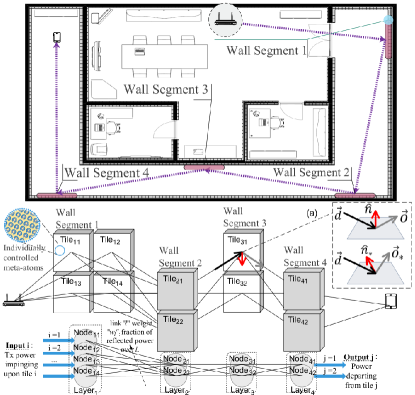
Figure 3: (Top): A natural/free grouping of complete SDM tile units is considered, e.g., per holding wall or wall segment. Each tile has individually controlled meta-atoms. A path of SDM groups to be traversed by TX-emitted waves is selected. (Middle): (a) Equivalent, virtual rotation of tiles, to match an impinging direction $\vec{d}$ to a required reflection direction $\vec{o}$. (Bottom) Neural network representation of the PWE.

We assume an environment with $N\left(\geq 2\right)$ pairs of transmitters (TXs) and receivers (RXs), with each link denoted with an index $n={1,2,...,N}$. With no loss of generality, all direct links from TXs to RXs are obstructed, which means that there is no line-of-sight (LOS) path among each pair of TX and RX, in order to focus our study on the configuration of the PWEs to maximize their utility. In each wall, the number of tiles, denoted as $\left\|\textrm{Wall}_{i}\right\|$ is generally larger than $N$ (i.e., $\left\|\textrm{Wall}_{i}\right\|>N$). The subscript $i$ represents the index of the wall and $\left\|*\right\|$ is the cardinality of the set of tiles of the corresponding wall. The set of tiles are expressed as $\{\textrm{Tile}_{ij}:i\in\mathbb{N},j\in\mathbb{N}\}$, where $j$ is the index of tile of the $i$-th wall, with each tile has a distinctly indexed.

III-A Configuration of a PWE as a Fully Connected Neural Network

III-A1 Structuring a NN for PWEs

The proposed neural network architecture sets as a primary goal to be directly interpretable, as shown in Fig. 3. We define that: i) each neuron (hidden or not) will represent exactly one physical SDM tile unit, and ii) the state of a neuron will directly correspond to a parameterized tile EM functionality.

For point (i), we begin by defining the number of layers and number of nodes in each layer. The number of layers corresponds to the number of walls (which have SDM tile coating) that a TX-emitted wave will sequentially impinge upon to reach an intended RX. Hence, for each TX-RX pair, the first step is to select the two SDM-coated walls in direct proximity of the TX and RX, respectively, which are mapped to the input and output layers of the neural network.

For point (ii), we employ a NN architecture which is qualitatively as close as possible to the actual physical propagation phenomenon. Thus, since tiles manipulate the flow of EM waves from a TX to an RX, we employ a feedforward NN since it enforces the same, similar activation and actuation of its neurons. Backpropagation is employed to re-tune the nodes (and corresponding tile functionalities) based on the received power pattern at the output layer at the previous feedforward step. A linear ramp will act as the node activation function, in order to be aligned with energy conservation principle of wireless propagation (i.e., the reflected power from a tile should be equal to the impinging one, in the ideal case). Any link weight will represent the portion of the tile-impinging energy that is reflected towards the link direction.

We proceed to study and details these design principles further.

III-A2 Mapping a PWE into a NN

The mapping process of SDM tiles into neural network nodes is visualized in Fig. 3. First, we assume a grouping of tiles into larger groups for scalability reasons. This grouping can be defined freely. For instance, since SDM tiles cover floorplan walls, one can naturally group together tiles that are placed over the same wall. Second, an order (path) of SDM groups is selected to serve as a coarse air-path connective the TX to the RX. This ordering is derived via any path finding algorithm (e.g., shortest path), over a graph comprising SDM groups as vertexes and SDM groups in LOS as edges. An example is shown in Fig. 3-top and Fig. 3-middle insets. Notice that the first group in this order is the one right after the TX. This group is deterministically set as the group of SDM tiles that receive TX-emitted waves impinging upon them. This information can be derived via the direct sensing capabilities of the SDM tile hardware [39]. Thus, the number of tiles in the first group and their identity is set. As a rule of a thumb, all subsequent groups are assumed to contain an equal number of SDM tile to the first layer. Finally, the ordering of groups is mapped to the neural network shown in Fig. 3-bottom inset. Each group is mapped to a neural network layer, and each specific SDM tile to a neural network node. A neural network link is inserted for each SDM tile pair within LOS of each other. The first group is the input layer and the last group is the output layer of the neural network.

The selection of intermediate layer-walls follows the principles of the KpConfig approach [5], summarized as follows. Since ideal SDMs can freely redirect any impinging direction to any other, the wave propagation becomes akin to routing in graph comprising SDM-coated walls as vertexes and links between walls within LOS of each other. The selection of intermediate walls follows a shortest-path finding procedure over this graph. All available tiles in selected walls over this shortest path become nodes of the corresponding wall-layer.

After determining the NN layers, the nodes/tiles per wall are selected. It is assumed that when the electromagnetic waves emitted from the TX impinge on the first wall, each tile in the first wall receives certain power, which is a function of the distance between the TX and the tile and the angle of arrival and can be treated as the “input” of the neural network. All tiles in the neural network can be tuned to redirect, split and focus its impinging power to other walls and tiles in their line-of-sight, as shown in black dashed lines in Fig. 3. The tiles reflect waves in tunable elevation and azimuth planes (a detailed discussion is provided below). After waves propagate via all wirelessly “connected” tiles, they reach the final wall-layer via multiple paths. The reflections from the final wall to the UE (User Equipment) is considered as the final “output”. Ideally, the final output received by the UE after reflections within the PWEs should be the transmitted power minus any path losses and any SDM reflection losses (which can be near-zero for ideal metasurfaces [40]). Hence, we can obtain a metric of deviation which is also the cost function of the proposed neural network, denoted as $\xi$, from the ideal output and actual measured values through different configurations of tiles. The root mean square error (RMSE) constitutes a common choice for $\xi$.

It is noted that metasurfaces can focus a wave as well as steer it towards an intended direction, which a degree of efficiency that is unique to metasurfaces over reflectarrays and antenna arrays. This capability can counter-balance the free-space path loss with a corresponding loss-canceling reflection gain. Thus, the overall path loss is essentially defined by any power consumed over the metasurface materials per each bounce [5].

Remark 1.

Essentially, the steering of a wave impinging on an SDM tile from a direction $\vec{d}$ to a reflected direction $\vec{r}$, is modeled as inducing a corresponding alteration to the vector $\hat{n}$, as shown in Fig. 3-(a). This convention was introduced in [5] and is denoted as virtual rotation of the normal $\hat{n}$. This means that the physical orientation of the SDM is not altered, but rather the SDM configuration acts as if the tile was rotated in a corresponding fashion to cause the intended reflection.

Note that the signals impinging on a tile can be scattered to more than one directions, depending on directions of arrival and the configuration of the tile. We describe this partial scattering of power over a set of reflection directions $\overrightarrow{o}$ using a heuristic power fraction $w_{\vec{o}}\left(\hat{n},\vec{d}\right)$, expressed as:

$$w_{\vec{o}}\left(\hat{n},\vec{d}\right)=\frac{\max\left\{\vec{r}\left(\hat{n},\vec{d}\right)\cdot\vec{o},0\right\}}{\sum_{\forall\vec{o}}w_{\vec{o}}},$$ (1)

in which $\vec{o}$ is the outgoing direction, $\vec{r}$ the reflecting direction, $\vec{d}$ the impinging direction. The projection of $\vec{r}$ over $\vec{o}$ is normalized across all outgoing links, assuming that $\vec{o}$ and $\vec{d}$ are unit vectors. A negative inner product implies that vectors $\vec{r}$, $\vec{o}$ are not aligned in the same direction and, thus, $w_{\vec{o}}$ should intuitively be zero.

According to the comparison result, the virtual rotation of the normal of each tile defines the reflected wave direction, obtained via the standard rule for calculating a reflection $\vec{r}$ from an impinging vector $\vec{d}$ and a surface normal $\hat{n}$:

$$\vec{r}\left(\hat{n},\vec{d}\right)=\vec{d}-2\left(\vec{d}\cdot\hat{n}\right)\hat{n},$$ (2)

Thus, $\hat{n}$ can be updated to minimize the cost function $\xi$:

$$\xi\left(\hat{n},\vec{d}\right)=\frac{1}{2}\sum_{l=1}^{L}\left(\bar{p}-\rho_{l}\left(\hat{n},\vec{d}\right)\right)^{2},$$ (3)

where $\bar{p}$ is the ideal output power value which is equal for each tile, $\rho_{l}$ the actual output power of the $l$-th tile within a wall of $L$ tiles, and $\rho_{l}\left(\hat{n},\vec{d}\right)=w_{\vec{o}}\left(\hat{n},\vec{d}\right)\cdot\bar{p}$.

III-B Rotation Matrices in PWEs

In order to describe a rotation of an object from its original orientation, several approaches are known: Euler angles, rotation axis and angle, quaternions, and rotation matrix [41]. Among all these methods, the rotation matrix is the most suitable for the tile rotations in PWEs, since even though it has the expression of $3\times 3$ matrices, it only introduces one parameter per plane, i.e., a rotation angle, to describe the rotation in the space. Additionally, since the tile normals are unary vectors, the effective degree of freedom for their virtual rotation is reduced to two (i.e., an azimuth and elevation defining the end-point of $\hat{n}$ over a sphere with unary radius, and an origin at the tile center). Therefore, to quantify the rotation of tiles in Euclidean space, we introduce the rotation matrices from linear algebra in a three-dimensional Cartesian coordinate system. In cases with no rotation, the normal vector of a plane $\hat{n}$ after normalization are:

$$\hat{n}_{\textsc{xz}}^{\pm\textsc{y}} =[0\quad\pm 1\quad 0]^{\intercal},$$

$$\hat{n}_{\textsc{yz}}^{\pm\textsc{x}} =[\pm 1\quad 0\quad 0]^{\intercal},$$

$$\hat{n}_{\textsc{xy}}^{-\textsc{z}} =[0\quad 0\quad-1]^{\intercal},$$

where the subscript of each $\hat{n}$ indicates the plane which the normal vector belongs to, and the superscript shows the pointing direction of the normal vector. Based on observations from previous studies [4, 27], we make the following remark regarding the effective rotation matrices:

Remark 2.

The tiles rotate virtually in only two planes, thus having two degrees of freedom. A tile fixed at the $xz$ plane has effective rotations around the $x$ and $z$ axes only.

The rotation matrices $R_{XZ},\,R_{YZ},R_{XY}$ are:

$$\begin{bmatrix}\cos\phi&-\sin\phi&0\\ \cos\theta\sin\phi&\cos\theta\cos\phi&-\sin\theta\\ \sin\theta\sin\phi&\sin\theta\cos\phi&\cos\theta\end{bmatrix},\\ \begin{bmatrix}\cos\varphi\cos\phi&-\cos\varphi\sin\phi&\sin\varphi\\ \sin\phi&\cos\phi&0\\ -\sin\varphi\cos\phi&\sin\varphi\sin\phi&\cos\varphi\end{bmatrix},\\ \begin{bmatrix}\cos\varphi&0&\sin\varphi\\ \sin\theta\sin\varphi&\cos\theta&-\sin\theta\cos\varphi\\ -\cos\theta\sin\varphi&\sin\theta&\cos\theta\cos\varphi\end{bmatrix}$$ (4)

respectively, where $\theta$, $\phi$, and $\varphi$ are the angles of rotation around the x, z, and y axis. It is worth noting that the rotation matrix is actually readily extendable to planar walls which might not be perpendicular to any Cartesian plane. The straightforward solution is to multiply the walls’ own orientation matrix to the tiles, then the rest of the procedure holds. Having a quantifiable metric for tile rotations $\hat{n}$, the power fraction calculation can be rewritten as

$$w_{\vec{o}}\left(\theta,\phi,\varphi,\vec{d}\right)=\frac{\max\left\{\vec{r}\left(\theta,\phi,\varphi,\vec{d}\right)\cdot\vec{o},0\right\}}{\sum_{\forall\vec{o}}w_{\vec{o}}}.$$ (5)

Remark 3.

In accordance with Remark 1, the reflection $\vec{r}\left(\theta,\phi,\varphi,\vec{d}\right)$ in relation (5) is defined by a virtual rotation of the unit surface normal $\hat{n}$. In a 3D setting, any such virtual rotation can be obtained just from an azimuth and elevation angle relative to the actual normal. As such, any two of the $\theta,\phi,\varphi$ angles can be selected for the operation of the described neural network, even on a per tile/node basis.

Figure 4: Multi-link PWEs with two pairs of TX and RX. No line-of-sight link can be found between the pairs.

III-C Ensemble Neural Networks for Multi-link PWEs

In PWEs with a multi-link scenario comprised of multiple walls, multiple pairs of TX and RX can be served with minimal interference. Suppose in a multi-link scenario, as illustrated in Fig. 4, the $l$-th tile which is located at the $k$-th wall and serves the $n$-th link has the power of the reflecting EM waves as:

$$\rho_{j}^{(k,l,n)}=\sum_{\forall\vec{d}_{i}}w_{\vec{o}}\left(\theta_{i,n},\phi_{i,n},\varphi_{i,n},\vec{d}_{i}\right)\cdot P_{i}^{(k,l,n)},$$ (6)

which is the feeding input power to the next layer (i.e., wall). At the final layer ($k=K$), the metric of deviation $\xi_{n}$, is calculated as:

$$\xi_{n}=\frac{1}{2}\sum_{\forall l}\left(\bar{\rho}^{(k,l,n)}-\rho^{(k,l,n)}\right)^{2}=\frac{1}{2}\sum_{\forall l}\delta_{l}^{2},$$ (7)

where $\bar{\rho}$ denotes the ideal output power ratio, and:

$$\delta_{l}=\bar{\rho}^{(k,l,n)}-\rho^{(k,l,n)}.$$ (8)

The reason for using ensemble neural networks for multi-link case is that ensemble learning can reduce the variance of predictions and minimize the error from multiple neural network models. The ensemble learning approach can be grouped by elements with variable values, such as different rotation matrices, number of tiles (nodes), and various activation functions. The nonlinear activation function can be hyperbolic tangent, softmax, or rectified linear unit (ReLU). Inside the ensemble structure, there are multiple parallel neural networks which follow the backpropagation rules to update the weights. After the feedforward links between wall-layers have been iterated until the final layer, each tile-node at each wall-layer (in reverse order) deduces the effect of its current rotation angles $\theta,\phi,\varphi$ to the deviation $\xi$, and updates $\theta,\phi,\varphi$ to a new set of values $\theta_{\ast},\phi_{\ast},\varphi_{\ast}$ . The corresponding update rule can be generalized as

$$\theta_{\ast}^{(k,l,n)} =\theta^{(k,l,n)}-\eta\cdot\left(\frac{\partial\xi}{\partial\theta}\right)^{(k,l,n)}\cdot\mathcal{S}^{(k,l,n)},$$

$$\phi_{\ast}^{(k,l,n)} =\phi^{(k,l,n)}-\eta\cdot\left(\frac{\partial\xi}{\partial\phi}\right)^{(k,l,n)}\cdot\mathcal{S}^{(k,l,n)},$$

$$\varphi_{\ast}^{(k,l,n)} =\varphi^{(k,l,n)}-\eta\cdot\left(\frac{\partial\xi}{\partial\varphi}\right)^{(k,l,n)}\cdot\mathcal{S}^{(k,l,n)},$$

where $\eta\in(0,1]$ is the network’s learning rate, and $\mathcal{S}^{(k,l,n)}$ is a factor denoting the significance of tile $(k,l)$ in the $n$-th link.

Note that given the remark made earlier, each update does not change all three rotation angles: only two of them will be updated based on the tile’s location. For the final wall-layer $k=K$ we define that $\mathcal{S}^{(K,l,n)}=\delta_{l}$, representing its deviation from the local ideal output. For $k\neq K$ we define it as the total power impinging on the tile, which is $\mathcal{S}^{(k,l,n)}=\sum_{\forall i}P_{i}^{(k,l,n)}$.

Inputs/Outputs. The input to each tile of the first layer is the normalized portion of power impinging upon it via the $\overrightarrow{d}$ links of user TX. Since the objective is to transfer all emitted power to user RX, these inputs can be virtual (i.e., not equal to the actual impinging power distribution). Thus, each input is set to $\nicefrac{{1}}{{K}}$ of the total emitted power, for each of the $K$ tiles in the first layer (i.e., the first “wall” after the TX). Using the same principle, the ideal output is set to $\nicefrac{{1}}{{K^{*}}}$, with $K^{*}$ being the number of tiles in the last layer (i.e., before the RX). Since the inputs and outputs remain the same at every feed-forward/back-propagate cycle, a high learning rate can be selected (e.g., $\eta=0.95$).

Implementing the feedforward / backpropagate process. The work of [29] introduced the formulation of $\left(\frac{\partial\xi}{\partial\phi}\right)^{(k,l,n)}$ in the $\xi$: RMSE case. The formulation yielded a custom feedforward / backpropagate implementation that operates at each node/tile, updating the corresponding virtual normal $\hat{n}\left(\phi,\theta\right)$ based on the status of the right-hand connected nodes. The corresponding right-hand neural links are then set based on relation (5).

However, it is noted that this custom implementation approach is not be directly compatible with the existing array of neural network software and hardware suites, which operate at the link-level, rather than at the node-level. Therefore, in this iteration of the scheme we propose an adaptation that provides compatibility with feedforward / backpropagate implementations operating at the link-level. Assuming any link update process, and once the corresponding right-hand link weights–$\mathring{w_{\overrightarrow{o}}}$–of a node have been updated, we introduce the following steps:

• From relation (5), calculate the virtual normal rotation, $\hat{n^{*}}$, that best matches the updated right-hand weights, i.e.,

  $$\hat{n^{*}}\leftarrow\text{argmin}_{\hat{n}}\xi\left(w_{\vec{o}}\left(\hat{n},\vec{d}\right)-\mathring{w_{\overrightarrow{o}}}\right),$$ (9)

  where $\xi$ is an error norm such as the RMSE, while $w_{\vec{o}}\left(\hat{n},\vec{d}\right)$ is given in relation (1). Notice that the match is approximate in the general case.

• Then, we proceed by updating anew the right-hand weights of the node via relation (5), using the calculated value of $\hat{n^{*}}$.

Notice that weight adaptations are not uncommon in neural networks in general. For instance, weight freezing–the process of excluding certain links from the weight update process–can be implemented by calculating a new link weight in the bulk of the training cycle, but eventually not updating its previous value [42].

These feed-forward/back-propagate cycles in each neural network can be executed in an online or offline manner, the ensemble learning process will finish until the deviation $\xi$ arrives at its global optimum, reaches an acceptable level or an allocated computational time window expires. At this point, the PWE controller simply deploys EM functionalities at each tile $(k,l)$ of each link, matching the attained $w_{\vec{o}}\left(\theta,\phi,\varphi,\vec{d}\right)$ values.

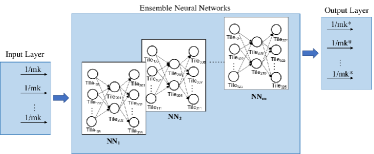
Figure 5: Structure of the proposed ensemble neural networks to enable global optimization over a large number of tiles/nodes.

Constructing Ensemble Neural Networks. In cases where a single layer-wall is too large to construct a single neural network with all nodes fully connected, an ensemble neural network can relieve the computational burden. As shown in Fig. 5, a total of $m$ fully connected neural networks are constructed with subsets of available tiles from wall-layer. The same input values (i.e., $1/(mk)$ due to the presence of $m$ neural networks) are injected to each node in the first hidden layer of each neural network. In the each neural network, a subset of tiles are selected for training. For example, in Fig. 5, each of the first and third layer has 25 tiles while the second has 10, a total of $m=5$ neural networks constitute an ensemble neural network to search for the optimal configuration of each tile NNConfig. Accordingly, the desired output value from each output layer becomes $1/(mk^{\ast})$.

III-D Interpretability: Mapping a trained neural network to tile configurations

As described in the context of relation (5), the feedforward process of NNConfig is not an accurate representation of the wave propagation process. Instead, for the sake of having a simplified computational rule that runs on each node of the neural network, relation (5) enforces a link weight derivation based on a simple projection of a wave reflection (derived from an incoming direction, $\vec{d}$, and the virtual tile surface normal, $\hat{n}$), over each outgoing direction, $\vec{o}$. Therefore, once the NNConfig network has been trained, its outcomes must be mapped to actual tile configurations that reflect the expected propagation outcome.

To this end, we consider a single trained neural network node and its corresponding tile. Let:

$$\vec{d}_{i},\,i=1\ldots D:\,w\left(\vec{d}_{i}\right)\neq 0$$ (10)

be the set of tile links that carry wireless waves with non-zero power that impinge over the tile, according to the NNConfig training outcome. Similarly, let:

$$\vec{o}_{i},\,i=1\ldots O:\,w\left(\vec{o}_{i}\right)\neq 0$$ (11)

be the set of tile links that carry wireless waves with non-zero power that depart from the tile. Additionally, let $\left\|*\right\|$ be the cardinality of a set $*$. Then, the following cases are defined:

• Case $\left(\left\|\vec{d}_{i}\right\|=1\right)\,\&\,\left(\vphantom{\vec{d}_{i}}\left\|\vec{o}_{i}\right\|=1\right)$. This case reflects a simple wave steering scenario, where a wave impinging from direction $\vec{d}_{i}$ is redirected to direction $\vec{o}_{i}$, with a corresponding virtual normal $\hat{n}$. Thus, the interpreted tile function can be written as:

  $$\text{{Steer}}\left(\vec{d}_{1},\vec{o}_{1}\right)\to\hat{n}.$$ (12)

• Case $\left(\left\|\vec{d}_{i}\right\|\geq 1\right)\,\&\,\left(\vphantom{\vec{d}_{i}}\left\|\vec{o}_{i}\right\|=0\right)$. In this case, waves impinge upon the tile from one or more directions while no reflections are requested, yielding a wave absorption function:

  $$\text{{Absorb}}\left(\vec{d}_{i}\right).$$ (13)

  From a physical standpoint of view, it is noted that wave absorption is perfect (i.e., yielding practically near-zero reflections) only when $\left\|\vec{d}_{i}\right\|=1$ [40]. When $\left\|\vec{d}_{i}\right\|>1$, absorption may be partially effective and lead to a degree of wave scattering. In that case, we apply:

  $$\text{{Absorb}}\left(\vec{d}_{I}\right),\,I:argmax_{i}\left(w\left(\vec{d}_{i}\right)\right),$$ (14)

  i.e., configuring the tile for absorbing perfectly the strongest impinging wave.

• Case $\left(\left\|\vec{d}_{i}\right\|=1\right)\,\&\,\left(\vphantom{\vec{d}_{i}}\left\|\vec{o}_{i}\right\|>1\right)$. In this case, a single impinging wave is reflected towards multiple directions, each carrying a portion of the original power. This functionality is known as splitting, i.e.:

  $$\text{{Split}}\left(\vec{d}_{1},\left\langle\vec{o}_{i},w\left(\vec{o}_{i}\right)\right\rangle\right)$$ (15)

• Case $\left(\left\|\vec{d}_{i}\right\|>1\right)\,\&\,\left(\vphantom{\vec{d}_{i}}\left\|\vec{o}_{i}\right\|>1\right)$. This constitutes the most general wave scattering case, which may not always have a unique mapping to a tile functionality. For instance, this scattering may be attributed to a splitting function (such as the one in relation (15)), when the tile is also illuminated by waves incoming from directions other than the intended one. Similarly, another possible cause of this scattering is to have a single steering–as defined in equation (12)–while the tile gets illuminated once again by one or more unintended incoming directions. Since the main goal of the proposed NNConfig is to use a single tile functionality for multiple connectivity objectives, this case will be mapped based on two principles: i) ensure at least one strong connection from set $\vec{d}_{i}$ to set $\vec{o}_{i}$, ii) pick the one specific connection that best fits the total sets $\vec{d}_{i}$ to $\vec{o}_{i}$. This is expressed as:

  $$\exists\hat{n}:\,\forall\vec{d}\in O_{d}\left(\vec{d_{i}}\right),\forall\vec{o}\in O_{o}\left(\vec{o_{i}}\right):\text{{Steer}}\left(\vec{d},\vec{o}\right)\to\hat{n}.$$ (16)

  In other words, there exists a steering functionality that reflects each indexed element of $O_{d}\left(\vec{d_{i}}\right)$ to the element of $O_{o}\left(\vec{o_{i}}\right)$ with the same index, for some orderings $O_{d}$, $O_{o}$ of the original sets.

  1:procedure MultiSteerMap(${\vec{d}}_{i}$,${\vec{o}}_{i}$)

  2:     $best\_score\leftarrow\infty;$

  3:     $best\_pair\leftarrow\emptyset;$

  4:     for $\overrightarrow{d}$ in $\overrightarrow{d}_{i}$

  5:       for $\overrightarrow{o}$ in $\overrightarrow{o}_{i}$

  6:         $\hat{n}{\scriptscriptstyle\leftarrow}\text{{Steer}}\left(\vec{d},\overrightarrow{o}\right)$;

  7:         $Set\,S\leftarrow\text{{CopyOf}}\left(\overrightarrow{o}_{i}\right);$

  8:         for $\overrightarrow{\delta}$ in $\overrightarrow{d}_{i}$

  9:           $S\leftarrow S-\left(\overrightarrow{\delta}-2\left(\overrightarrow{\delta}\cdot\hat{n}\right)\hat{n}\right);$

  10:         end for

  11:         if $\left\|S\right\|<best\_score$ then

  12:           $best\_score\leftarrow\left\|S\right\|;$

  13:           $best\_pair\leftarrow\left\langle\overrightarrow{d},\overrightarrow{o}\right\rangle$

  14:         end if

  15:       end for

  16:     end for

  17:     return $best\_pair$;

  Algorithm 1 The multi-steer interpretation process.

The definition of mapping (16) is strict, in the sense that there may not exist an $\hat{n}$ that meets it precisely. Therefore, the MultiSteerMap process (Algotihm 1) presents a practical, approximate heuristic. The algorithm goes through all possible incoming/outgoing direction pairs, and considers the prospects of deploying the corresponding Steer function. The pair that leads to the connectivity of the most $\vec{d}_{i}$ to $\vec{o}_{i}$ elements is finally selected.

For the sake of completion we also mention the case where $\left(\left\|\vec{d}_{i}\right\|=0\right)\,\&\,\left(\vphantom{\vec{d}_{i}}\left\|\vec{o}_{i}\right\|\geq 1\right)$, i.e., a tile with zero impinging power and non-zero reflected one, which is an invalid case. Note that this trained node outcome is naturally prohibited from the training process, due to the form of relation (5).

As explained in [5], certain metasurface functionalities are disjoint and independent from others. The most critical functionality is to steer RF power and guide it to an RX. This is accomplished by the proposed scheme, citing the more economic use of tiles versus the scheme of [5], i.e., using fewer tiles to serve a given set of users. The output is one or more “air-routes” connecting the emissions of a TX to an RX.

Subsequent metasurface functionalities, i.e., polarization alteration and phase alteration can be applied to any “air-route” at the final step of the PWE configuration. Just one tile per “air-path” can be used to introduce a phase shift or a polarization rotation per air-path, without affecting the steering outcome deduced by the proposed NNConfig, as discussed in [5]. We note that, in this manner, phase and polarization control can be set deterministically (e.g., to cancel fading effects) and they need not be subject to a heuristic optimizer such as a neural network.

Regarding the frequency control, metasurfaces can indeed act as frequency filters, but are usually not tunable in that sense. In other words, when activated, a metasurface filters impinging frequencies, while it does not do so when remaining inactive. As such, this functionality is not taking into account into the neural network either.

Finally, regarding the obstacle avoidance, NNConfig receives as input a series of walls that form a path which bypasses LOS obstacles. (Note that avoiding malevolent users and protecting floorplan areas from interference can be treated similarly). This series of walls is derived via path-finding algorithms (e.g., K-Shortest Paths [5]) within a graph constructed as follows: walls are mapped to graph nodes and walls within LOS of each other are mapped to graph-links. This path-finding functionality is already used in KpConfig [5] and is re-used in this work as input.

Ultimately, the approximate TX/RX user device position is treated as an input provided by external services (as shown in Fig. 1 and its discussion). The neural network training criterion is the RX received power, and as such any uncertainty in the device locations is handled automatically by the neural network training process to the extend possible.

IV Evaluation

We evaluate the performance of NNConfig in the PWE simulator presented in [5]. We seek to evaluate the potential of the proposed scheme in a ray-tracing setting, from the aspects of: i) receiver signal power levels, ii) neural network training, and iii) tile numbers usage.

We compare its outcomes to the KpConfig scheme for PWEs presented in [5] and whose operation has been outlined in Section II. To the best of our knowledge, KpConfig is the only scheme that operates at the PWE configuration layer (i.e., definition of wave steering commands) and, therefore, directly comparable to the proposed NNConfig.

As explained in the context of Fig. 3, NNConfig receives as input a series of tile sets (walls), which act as the neural network layers. (In the context of this evaluation, this is accomplished by executing KpConfig, which produces end-to-end tile-disjoint paths between the RX and the TX, as shown in Fig. 7a. Any KpConfig-derived tile functionality is then discarded, and we keep only the same-wall tiles, which act as the NNConfig nodes and layers, as shown in Fig. 3). In order to evaluate the NNConfig for varying number of hidden layer cases, we consider the floorplan scenarios shown in Table I. In scenario 1, propagating waves necessarily need to impinge upon 1 hidden layer (i.e., NLOS wall), with the LOS walls of the TX and the RX acting as the input and output layers respectively, producing a neural network with a total of 3 layers, i.e., $5\times 5\times 5$ assuming 5 tiles per wall. Similarly, we have a NN of $5\times 5\times 5\times 5$ for scenario 2, $5\times 5\times 5\times 5\times 5$ for scenario 3, $5\times 5\times 5\times 5\times 5\times 5$ for scenario 4, and $5\times 5\times 5\times 5\times 5\times 5\times 5$ for scenario 5. In general, scenario $I$ corresponds to $I$ hidden neural network layers and $I+2$ layers total. The tile numbers within each layer are defined as $\left(\text{tiles\,over\,wall-layer}\right)\times\left(\text{NN pruning factor}\right)$, where NN pruning is a factor introduced for experimenting with a variable ensemble neural network structure. Apart from this variable change in the node numbers per layer, all other ensemble parameters are identical to those defined above.

TABLE I: Floorplan, user location and beam orientation coordinate system. The origin is at the lower left corner of the floorplan.

User: Position, $\alpha$,$\phi$,$\theta$ TX(0): [2.5, 7.5, 1.5], 40o, 0o, 0o RX(1): [$L$-2.5, 7.5, 1.5], 40o, 0o, 180o       $L$: floorplan total width Comm. Pair: TX(0)$\to$RX(1) Objective: Max. RX Power
Five floorplans studied (with increasing number of middle-walls from one to five).

TABLE II: Simulation parameters.

Ceiling Height	$3$ $m$
Tile Dimensions	$1\times 1\,m$ (z-centered)
Tile Functions	Steer, Split, Focus, Absorb
Non-SDM surfaces	Perfect absorbers (cf. red in Table I)
Frequency	$2.4\,GHz$
TX Power	$-30\,dBm$
Antenna type	Single $a^{o}$-lobe sinusoid,
	pointing at $\phi^{o},\theta^{o}$ (cf. Table I)
Max ray bounces	$50$
Power loss per bounce	$1$ %
NN training cycles	$10,000$
NN optimization	Gradient with momentum
NN pruning factor range	20% : 20% : 100%

In each floorplan we consider a TX-RX pair as shown in Table I. For ease of exposition, i.e., in order to provide meaningful illustrations of the actual wireless propagation, SDM-covered surfaces are denoted as black-colored walls, thereby confining the tile-sets produced by KpConfig into these locations. We seek to tune each SDM tile in this setup so as to maximize the received power at the RX. It is noted that, based on the KpConfig workflow, in a multi-user scenario each pair is treated sequentially, i.e., walls are defined by KpConfig, then one neural network is created and trained by NNConfig, finally configuring the corresponding tiles. The process repeats for each pair, each time considering any previously configured tiles as frozen, i.e., subject to no further training in the neural network sense. Thus, the single-pair scenario performance reflects the core, repeating process which is also coupled with ease of exposition benefits.

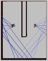
(a) KpConfig propagation.

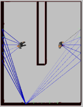
(b) NNConfig propagation.

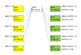
(c) Trained neural network corresponding to Fig. 6b.

Figure 6: KpConfig and NNConfig behavior at the 1-middle wall floorplan case. In KpConfig-derived propagation, individual paths fully occupy available tiles, whereas in NNConfig-derived propagation only the single-best tile is selected which improves received power and link efficiency.

Table II summarizes the persistent simulator parameters across all subsequent tests. As in [5], each Steer or Split function is coupled with a wave Focus function at the same direction. Focus essentially counter-balances the free-space path loss by a corresponding reflection gain, which is a unique capability of metasurfaces over reflectarrays and phased array antennas. Thus, the overall path loss is essentially defined by any power consumed over the metasurface materials per each bounce [5]. This loss has been shown to take very small values, at the order of 1% [40]. The NN pruning factor is an input variable (common for all neural network layers), whose studies range is 20% to 100% with steps of 20%.

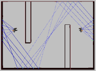
(a) KpConfig propagation.

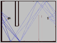
(b) NNConfig propagation.

Figure 7: KpConfig and NNConfig behavior at the 2-middle wall scenario. The utilization of NNConfig maintains full link connectivity while reducing deployment of five tiles, compared with the same link using KpConfig.

Once the neural network is created, the inputs and ideal outputs are set to their values, as described in Section III-C. We employ the root mean square error (RMSE) as the deviation $\xi$ between the ideal outputs and the training outcomes in each cycle. The initial $\theta,\,\phi$ angle values (azimuth and elevation of the virtual normal) per neural node are randomized in the ranges of $\left[-90^{o},90^{o}\right]$ and $\left[0^{o},90^{o}\right]$, respectively. Finally, the termination criterion is to reach $10,000$ feed-forward/back-propagate cycles, which is kept constant over all floorplan cases to ensure a constant runtime.

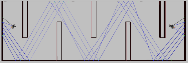
(a) KpConfig propagation.

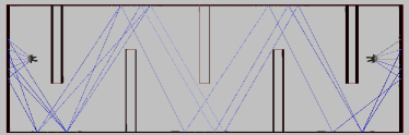
(b) NNConfig propagation.

Figure 8: KpConfig and NNConfig behavior at the 5-middle wall scenario. Such comparison in the number of deployed tiles demonstrates NNConfig’s advantage on link efficiency enhancement.

Figs. 6, 7, and 8 visualize the end-to-end propagation achieved by the proposed NNConfig and the KpConfig over the floorplans 1, 2, and 5, as identified by the number of middle walls. (Floorplans 3 and 4 convey similar conclusions and are omitted).

In the floorplan 1 case (Fig. 6), the KpConfig outcome (Fig. 6a) visualizes the disadvantage of this approach detailed in Section II: each user link is treated sequentially and connected to its end-point within a graph, resulting into a multitude of independent paths and full occupancy of all available tiles. On the other hand, NNConfig achieves in finding a propagation solution that employs just a single tile, with a MultiSteer functionality (Algorithm 1). Single Steer functionalities are necessarily applied to the tiles adjacent to the users in both schemes. The trained neural network is shown in Fig. 6c, which shows good correspondence with the mapped result of Fig. 6b.

In the floorplan 2 case (Fig. 7), KpConfig once again ensures connectivity by using up all available tiles (Fig. 7a). NNConfig manages to also achieve full connectivity while using 5 tiles less, by employing 4 MultiSteer functionalities. In the floorplan 5 case (Fig. 8), which potentially constitutes an extreme scenario, KpConfig exhibits the same behavior, i.e., full connectivity and full tile occupancy (Fig. 8a). NNConfig pinpoints several MultiSteer functionalities, combining the transmitting user’s emissions over much fewer tiles towards the receiver (Fig. 8b). It is worth noting that the air-paths demonstrate a pattern of “two-cluster” formation in Figs. 7b and 8b, the reason for such coincidence is due to the symmetries of the two floorplans and is not a deterministic input to the NNConfig.

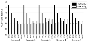
Figure 9: Received power per compared scheme over the studied floorplans. The y-axis is in negative $dBmW$ (i.e., lower is better). The $20-100$ percentage represents the neural network pruning factor.

The absolute received power performance of the compared schemes is shown in Fig. 9. Notably, the performance of KpConfig depends strongly on the the neural network pruning factor: higher factor values (i.e., neural network layers containing more nodes) favor the KpConfig performance, and is repeated across all floorplan scenarios. This is a natural outcome, given that KpConfig does not reuse tiles, i.e., one tile serves exactly one impinging wave direction, as shown in Fig. 6a. Removing a tile leads to a proportional reduction in the successfully steered (and RX-received) wireless power. NNConfig exhibits weaker dependence from the pruning factor, and received power near the KpConfig best case. In fact, NNConfig benefits from low factor values (i.e., neural network layers containing less nodes), since the algorithm is pushed to: i) find PWE configurations with increased tile reuse, and ii) a smaller neural network is likely to be trained better in allotted time. It is noted that the received power in the non-PWE case (no SDMs) is below $-150\,\text{dBmW}$ in all floorplans.

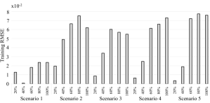
Figure 10: Training Root Mean Square Error for NNConfig over the studied floorplans.

To better understand the remarked behavior of NNConfig we turn to Fig. 10. Setting a static limit to the neural network training cycles (cf. Table II) yields an increase in the training RMSE, given the increasing network size per floorplan. However, this error is almost inconsequential to the overall performance, as was shown in the context of Fig. 9. This is due to the fact that the neural network interpretation process is forgiving to link weight imprecisions owed to prematurely stopped training. In essence, the interpretation process of Section III-D revolves around node connectivity, rather than precise link weights. Thus, if the main neural paths have been established, the interpretation process will yield a good outcome, even if the link weights have not been fully optimized.

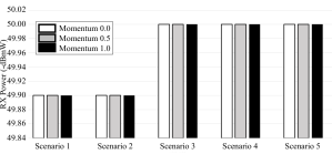
(a) Momentum independence (learning rate is $1.0$).

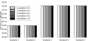
(b) Learning rate independence (momentum is $1.0$).

Figure 11: Validation of the independence of the NNConfig performance from the classic neural network training parameters (pruning factor is $20$%).

Regarding the neural network training process, as discussed in the Annex, we employ a standard feedforward/backpropagation operation [42], but alter the link weight deltas to comply with relation (23) at each step. In the general case, (i.e., not specialized to NNConfig) a backpropagation process updates the link weights at a given $step$ as:

$$w_{ji}^{\prime}\leftarrow w_{ji}-\eta\cdot\left(\frac{\partial\xi}{\partial w_{ji}}\right)_{step}-\mu\cdot\left(\frac{\partial\xi}{\partial w_{ji}}\right)_{step-1}$$ (17)

where $\eta$ is a learning rate factor and $\mu$ is the momentum factor attributed to the partial derivative for link $ji$ at the previous backpropagation step $t-1$, and then we alter the $w_{ji}^{\prime}$ . For the NNConfig-specialized process, we subsequently alter each $w_{ij}^{\prime}$ by a multiplicative factor $\eta_{ji}$, to ensure compliance with relation (23). This raises the question: do we need to optimize the factors $\eta$ and $\mu$ of the general update rule (17) for NNConfig (i.e., prior to weight adaptation)? In Fig. 11 we execute a parametric variation study of the received power for NNConfig in all five floorplan scenarios. Notably, the NNConfig performance exhibits no dependence on the factors $\eta$ and $\mu$. The required compliance with relation (23) essentially defines any multiplicative factor for the quantity $\frac{\partial\xi}{\partial w_{ji}}$, meaning that NNConfig does not need to be tuned in that aspect, discarding the dependence from two of the most common neural network parameters (learning rate and momentum) in general and limiting the size of its solution space.

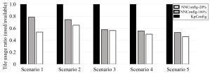
Figure 12: Ratio of SDM tiles used per compared scheme over the studied floorplans.

Limiting the tile occupancy ratio is important to the operation of a PWE for two reasons. First, it implies that the same PWE can serve more communicating user pairs, thereby yielding higher served user capacity [5]. Second, tiles are electronic devices that need to be powered and be in communication with the PWE server, resulting into electrical power consumption, as well as into computational and communication system overhead. Therefore, limiting their use is beneficial from these aspects. NNConfig presents considerable gains in number of tiles occupied, as shown in Fig. 12. In this Figure we compare KpConfig (pruning factor 100%) and NNConfig (pruning factor 20%) variations, since they yield the maximal received power for both algorithms (cf. Fig. 9). Moreover, we include the NNConfig (pruning factor 100%) to the comparison, to demonstrate the tile number-economic operation of NNConfig even in the worst case. NNConfig-100% uses 75% of the available tiles in the floorplan 1 case, a percentage that reduces to approximately 50% in the floorplan 5 scenario. In contrast, the KpConfig tile occupancy is always 100%. In essence, each scheme necessarily uses all tiles in the walls adjacent to the users (as these receive the users’ emissions), but differ in the use of tiles in the intermediate surfaces. Moreover, each floorplan naturally introduces more available tiles, due to the enlargement of the environment, as shown in Table I. Nonetheless, the NNConfig tile occupancy is low, at a level that the overall trend of the plot in Fig. 12 is to decrease. NNConfig-20% performs better overall, yielding the highest received power in Fig. 9.

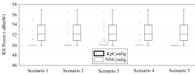
(a) Received power variation.

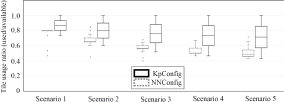
(b) Tile usage variation.

Figure 13: Performance variation of NNConfig and KpConfig over the complete range of pruning factor values (20%-100% step by 20%).

In the preceding experiments it was made evident that the pruning factor is the only input parameter of NNConfig which is potentially subject to optimization. Therefore, in Fig. 13 we study the performance variation of NNConfig and KpConfig over the complete range of the pruning factor given in Table II. Our goal is to evaluate the performance bounds assuming no means of optimizing the pruning factor. As shown in Fig. 13a, NNConfig exhibits limited RX power dependence: regardless in the number of available tiles is large, NNConfig will search for tile-reusing PWE configurations. Therefore, assuming enough runtime, the solution will be consistent and invariable. On the other hand, KpConfig is very sensitive to the pruning factor, as it is greedy in tile usage and the exclusion of tiles from the solution space can reduce the received power proportionately (cf. Fig. 6a and Fig. 9). Thus, the KpConfig variation is large and uniform across all floorplan scenarios. The tile usage variation in Fig. 13b follows the same rationale, and the trend is similar to Fig. 12.

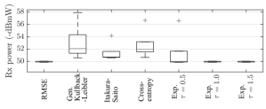
Figure 14: Performance variation of NNConfig for various cost functions.

Finally, in Fig. 14 we justify the use of RMSE as the cost function. After experimentation with several alternatives (listed in the x-axis of Fig. 14), RMSE and the exponential cost function, $\tau\cdot e^{\sum_{\forall l}\nicefrac{{1}}{{\tau}}\left(\delta_{l}\right)^{2}}$, behaved equally well in terms of yielding the best performance over all experiments and layout scenarios. Nonetheless, the exponential cost function requires the optimization of its tunable parameter $\tau$, while RMSE does not pose such a requirement.

V Conclusion

Intelligent surfaces allow for programmatic control over the wireless propagation phenomenon within a space, with novel capabilities in wireless link quality, security and power transfer. The largest the deployment of surface units within an indoor or outdoor space, the more deterministic the control over the wireless propagation as a whole, to the benefit of communicating users. The present study proposed a novel technique for such large scale configurations based on machine learning techniques. Particularly, a customized, interpretable neural network was proposed, where surface units are represented as neural network nodes, and connectivity as neural links. The neural network is required to yield ideal output, such as total signal delivery to the receiver, and back-propagation rules optimize the link weights accordingly. An interpretation process maps the trained links to intelligent surface configurations. The proposed scheme inherits the weaknesses of neural networks deriving from their heuristic nature: convergence guarantees within a given time interval cannot be given. As such, the scheme outputs should always be compared to simpler but deterministic solutions, and be adopted when clearly superior. Simulations showed that the proposed scheme can be synergistic to related schemes, and effectively use a single surface towards meeting multiple objectives, thus being economic in terms of total surfaces used for serving a set of users.

Assume a neural network with the following notation: i) $x_{ji}$– the $i^{th}$ input to node $j$, ii) $w_{ji}$– the weight associated with input $i$ to unit $j$, iii) $z_{j}$– the weighted sum of inputs for node $j$ ($z_{j}=\sum_{\forall i}w_{ji}\cdot x_{ji}$ ).

The linear ramp function will serve as the activation function and, thus, $z_{j}$ will also be equal to the output of node $j$. This simplifies the classic neural network derivatives as [42]:

$$\frac{\partial\xi}{\partial w_{ji}}=\frac{\partial\xi}{\partial z_{j}}\cdot\frac{\partial z_{j}}{\partial w_{ji}}=\frac{\partial\xi}{\partial z_{j}}\cdot x_{ji},$$ (18)

which holds in general. Additional simplifications are:

$$\frac{\partial\xi}{\partial z_{j}}=-\left(o_{j}-z_{j}\right)$$ (19)

for any output layer node and $\xi:\,RMSE$. For a hidden layer node $j$, we use the notation $\left\{\underset{\to}{j}\right\}$ to denote all nodes downstream of $j$ and indexed by $k$. These nodes are affected by the output of node $j$ and, therefore:

$$\frac{\partial\xi}{\partial z_{j}}=\sum_{\forall k\in\left\{\underset{\to}{j}\right\}}\frac{\partial\xi}{\partial z_{k}}\cdot\frac{\partial z_{k}}{\partial z_{j}}=\sum_{\forall k\in\left\{\underset{\to}{j}\right\}}\frac{\partial\xi}{\partial z_{k}}\cdot w_{kj}$$ (20)

Finally, for any node (output or hidden) we note the well-known weight update rule:

$$w_{ji}^{*}\leftarrow w_{ji}-\eta\cdot\frac{\partial\xi}{\partial w_{ji}}$$ (21)

where $\eta$ is a constant (commonly referred to as learning rate). $\frac{\partial\xi}{\partial w_{ji}}$ is derived from eq. (18) and (20) for hidden nodes, and via eq. (18) and (19) for output nodes. Up to this point, the solution space of $w_{ij}$ values is completely unrestricted: $w_{ij}$ values are completely disjoint.

Specializing for the neural networks studies in this paper, we derive from eq. (1):

• The weight values sourced from a node (downstream) need to be greater than zero and normalized, to respect the energy conservation principle:

  $$w_{\vec{o}_{k}j}^{*}\in\mathbb{R^{+}},\,\sum_{\forall\vec{o}}w_{\vec{o}_{k}j}^{*}\leq 1$$ (22)

  .

• The values sourced from a node (downstream) are fully defined by the node’s virtual norm $\hat{n}_{j}$, i.e., combining eq. (2) with (1) (omitting the $\max$ operator and the normalization for ease of exposition): $w_{\vec{o}_{k}j}^{*}=\vec{o_{k}}\cdot\sum_{\forall i}\left(\vec{d_{ji}}-2\left(\vec{d_{ji}}\cdot\hat{n_{j}}\right)\cdot\hat{n}_{j}\right),$reminding that $\vec{o_{k}}$ and $\vec{d_{ji}}$ are static and constant vectors, defined by the floorplan geometry ant SDM tile locations.

The virtual normal $\hat{n_{j}}$ is furthermore defined completely by any two of the rotation matrix angles $\left\langle\theta_{j},\phi_{j},\varphi_{j}\right\rangle$, as shown in eq. (5). For ease of exposition we will keep the pair $\left\langle\theta_{j},\phi_{j}\right\rangle$. Then, we can write that $w_{\vec{o}_{k}j}^{*}=\mathcal{F}_{\vec{o}_{k}j}\left(\theta_{j},\phi_{j}\right)$ with $\mathcal{F}$ denoting the relation specialized for each $\vec{o}_{k}j$ index. In other words, the weights are not free to take any values and are defined by $\left\langle\theta_{j},\phi_{j}\right\rangle$. As such, the update rule (21) needs to be updated accordingly as follows. Our entry-point will be the $\eta$ constant, which will be specialized for each $ij$ index as $\eta_{ij}$. We note that this practice is not uncommon: weight freezing approaches make use of this technique [42]. Finally, we set $\eta_{ij}$ as:

$$\eta_{ij}\leftarrow\arg opt_{\eta_{ij}}\left(w_{ji}-\eta_{ij}\cdot\frac{\partial\xi}{\partial w_{ji}}\right),\\ \text{{subject\,to}:}\\ \exists\left\langle\theta_{j},\phi_{j}\right\rangle:w_{ji}-\eta_{ij}\cdot\frac{\partial\xi}{\partial w_{ji}}=\mathcal{F}_{\vec{o}_{k}j}\left(\theta_{j},\phi_{j}\right),\forall j\\ \text{$\left(w_{ji}-\eta_{ij}\cdot\frac{\partial\xi}{\partial w_{ji}}\right)\in$$\mathbb{R^{+}}$,$\sum_{\forall\vec{o}}\left(w_{ji}-\eta_{ij}\cdot\frac{\partial\xi}{\partial w_{ji}}\right)\leq$1}$$ (23)

or in an approximate form as:

$$\eta_{ij}\leftarrow\arg\min_{\eta_{ij}}\left(\sum_{\forall j}\left|\left(w_{ji}-\eta_{ij}\cdot\frac{\partial\xi}{\partial w_{ji}}\right)-\left(\mathcal{F}_{\vec{o}_{k}j}\left(\theta_{j},\phi_{j}\right)\right)\right|\right),\\ \text{{subject\,to:}}\\ \left(w_{ji}-\eta_{ij}\cdot\frac{\partial\xi}{\partial w_{ji}}\right)\in\mathbb{R^{+}},\,\sum_{\forall\vec{o}}\left(w_{ji}-\eta_{ij}\cdot\frac{\partial\xi}{\partial w_{ji}}\right)\leq 1\,\,\,\blacksquare$$ (24)

References

- [1] I. F. Akyildiz, S. Nie, S.-C. Lin, and M. Chandrasekaran, “5g roadmap: 10 key enabling technologies,” Computer Networks, vol. 106, pp. 17–48, 2016.
- [2] T. Huang, W. Yang, J. Wu, J. Ma, X. Zhang, and D. Zhang, “A survey on green 6g network: Architecture and technologies,” IEEE Access, vol. 7, pp. 175 758–175 768, 2019.
- [3] S. Ghendir, S. Sbaa, A. Al-Sherbaz, R. Ajgou, and A. Chemsa, “Towards 5g wireless systems: A modified rake receiver for uwb indoor multipath channels,” Physical Communication, vol. 35, p. 100715, 2019.
- [4] C. Liaskos, S. Nie, A. Tsioliaridou, A. Pitsillides, S. Ioannidis, and I. Akyildiz, “A new wireless communication paradigm through software-controlled metasurfaces,” IEEE Communications Magazine, vol. 56, no. 9, pp. 162–169, Sept 2018.
- [5] C. Liaskos, A. Tsioliaridou, S. Nie, A. Pitsillides, S. Ioannidis, and I. F. Akyildiz, “On the Network-Layer Modeling and Configuration of Programmable Wireless Environments,” IEEE/ACM Transactions on Networking, vol. 27, no. 4, pp. 1696–1713, 2019.
- [6] J. Zhang, G. Zheng, I. Krikidis, and R. Zhang, “Specific absorption rate-aware beamforming in miso downlink swipt systems,” IEEE Transactions on Communications, 2019.
- [7] C. Liaskos, A. Tsioliaridou, A. Pitsillides, I. F. Akyildiz, N. V. Kantartzis, A. X. Lalas, X. Dimitropoulos, S. Ioannidis, M. Kafesaki, and C. Soukoulis, “Design and development of software defined metamaterials for nanonetworks,” IEEE Circuits and Systems Magazine, vol. 15, no. 4, pp. 12–25, 2015.
- [8] G. Oliveri, D. H. Werner, and A. Massa, “Reconfigurable electromagnetics through metamaterials – a review,” Proceedings of the IEEE, vol. 103, no. 7, pp. 1034–1056, 2015.
- [9] C. Huang, A. Zappone, G. C. Alexandropoulos, M. Debbah, and C. Yuen, “Reconfigurable intelligent surfaces for energy efficiency in wireless communication,” IEEE Transactions on Wireless Communications, vol. 18, no. 8, pp. 4157–4170, 2019.
- [10] X. Tan, Z. Sun, J. M. Jornet, and D. Pados, “Increasing indoor spectrum sharing capacity using smart reflect-array,” 2016 IEEE International Conference on Communications, ICC 2016, 2016.
- [11] Q. Wu and R. Zhang, “Intelligent reflecting surface enhanced wireless network,” arXiv:1809.01423, 2018.
- [12] S. Hu, F. Rusek, and O. Edfors, “Beyond massive mimo: The potential of data transmission with large intelligent surfaces,” IEEE Transactions on Signal Processing, vol. 66, no. 10, pp. 2746–2758, 2017.
- [13] L. Zhang, X. Q. Chen, S. Liu, Q. Zhang, J. Zhao, J. Y. Dai, G. D. Bai, X. Wan, Q. Cheng, G. Castaldi et al., “Space-time-coding digital metasurfaces,” Nature communications, vol. 9, no. 1, p. 4334, 2018.
- [14] C. Huang, S. Hu, G. C. Alexandropoulos, A. Zappone, C. Yuen, R. Zhang, M. Di Renzo, and M. Debbah, “Holographic mimo surfaces for 6g wireless networks: Opportunities, challenges, and trends,” arXiv preprint arXiv:1911.12296, 2019.
- [15] H. Han, J. Zhao, D. Niyato, M. Di Renzo, and Q.-V. Pham, “Intelligent reflecting surface aided network: Power control for physical-layer broadcasting,” arXiv preprint arXiv:1910.14383, 2019.
- [16] J. Zhao, “Optimizations with intelligent reflecting surfaces (IRSs) in 6G wireless networks: Power control, quality of service, max-min fair beamforming for unicast, broadcast, and multicast with multi-antenna mobile users and multiple IRSs,” arXiv preprint arXiv:1908.03965, 2019.
- [17] M. E. M. Cayamcela, S. R. Angsanto, W. Lim, and A. Caliwag, “An artificially structured step-index metasurface for 10ghz leaky waveguides and antennas,” in 2018 IEEE 4th World Forum on Internet of Things (WF-IoT). IEEE, 2018, pp. 568–573.
- [18] I. F. Akyildiz, C. Han, and S. Nie, “Combating the distance problem in the millimeter wave and terahertz frequency bands,” IEEE Communications Magazine, vol. 56, no. 6, pp. 102–108, June 2018.
- [19] S. Nie, J. M. Jornet, and I. F. Akyildiz, “Intelligent environments based on ultra-massive mimo platforms for wireless communication in millimeter wave and terahertz bands,” in ICASSP 2019-2019 IEEE International Conference on Acoustics, Speech and Signal Processing (ICASSP). IEEE, 2019, pp. 7849–7853.
- [20] F. Liu, O. Tsilipakos, A. Pitilakis, A. C. Tasolamprou, M. S. Mirmoosa, N. V. Kantartzis, D.-H. Kwon, M. Kafesaki, C. M. Soukoulis, and S. A. Tretyakov, “Intelligent metasurfaces with continuously tunable local surface impedance for multiple reconfigurable functions,” Physical Review Applied, vol. 11, no. 4, p. 044024, 2019.
- [21] C. Huang, G. C. Alexandropoulos, A. Zappone, M. Debbah, and C. Yuen, “Energy efficient multi-user miso communication using low resolution large intelligent surfaces,” in 2018 IEEE Globecom Workshops (GC Wkshps). IEEE, 2018, pp. 1–6.
- [22] C. Huang, G. C. Alexandropoulos, C. Yuen, and M. Debbah, “Indoor signal focusing with deep learning designed reconfigurable intelligent surfaces,” in Proc. of SPAWC’19, pp. 1–5.
- [23] C. Huang, R. Mo, C. Yuen et al., “Reconfigurable intelligent surface assisted multiuser miso systems exploiting deep reinforcement learning,” IEEE JSAC, pp. 1–12, 2020.
- [24] F. Samadi and A. Sebak, “Reconfigurable surface design for electromagnetic wave control,” in 2019 IEEE International Electromagnetics and Antenna Conference (IEMANTENNA). IEEE, 2019, pp. 025–028.
- [25] A. C. Tasolamprou, A. Pitilakis, S. Abadal, O. Tsilipakos, X. Timoneda, H. Taghvaee, M. S. Mirmoosa, F. Liu, C. Liaskos, A. Tsioliaridou et al., “Exploration of intercell wireless millimeter-wave communication in the landscape of intelligent metasurfaces,” IEEE access, vol. 7, pp. 122 931–122 948, 2019.
- [26] O. Tsilipakos et al., “Toward intelligent metasurfaces,” Advanced Optical Materials, p. 2000783.
- [27] C. Liaskos, S. Nie, A. Tsioliaridou, A. Pitsillides, S. Ioannidis, and I. Akyildiz, “Realizing wireless communication through software-defined hypersurface environments,” in 2018 IEEE 19th International Symposium on” A World of Wireless, Mobile and Multimedia Networks”(WoWMoM). IEEE, 2018, pp. 14–15.
- [28] C. Liaskos et al., “A novel communication paradigm for high capacity and security via programmable indoor wireless environments in next generation wireless systems,” Ad Hoc Networks, vol. 87, pp. 1–16, 2019.
- [29] C. Liaskos, A. Tsioliaridou, S. Nie, A. Pitsillides, S. Ioannidis, and I. F. Akyildiz, “An interpretable neural network for configuring programmable wireless environments,” in IEEE SPAWC 2019, 2019, pp. 1–5.
- [30] C. Liaskos, A. Tsioliaridou et al., “Initial uml definition of the hypersurface programming interface and virtual functions,” European Commission Project VISORSURF: Accepted Public Deliverable D2.1, 31-Dec-2017, [Online:] http://www.visorsurf.eu/m/VISORSURF-D2.1.pdf.
- [31] C. Liaskos, A. Pitilakis et al., “Initial uml definition of the hypersurface compiler middle-ware,” European Commission Project VISORSURF: Accepted Public Deliverable D2.2, 31-Dec-2017, [Online:] http://www.visorsurf.eu/m/VISORSURF-D2.2.pdf.
- [32] A. Pitilakis et al., “A multi-functional intelligent metasurface: Electromagnetic design accounting for fabrication aspects,” arXiv preprint arXiv:2003.08654, 2020.
- [33] The VISORSURF project, “A hardware platform for software-driven functional metasurfaces,” European Union CORDIS, Project report, pp. 15–35. [Online]. Available: https://ec.europa.eu/research/participants/documents/downloadPublic? documentIds=080166e5c560b376&appId=PPGMS
- [34] C. Liaskos, A. Tsioliaridou, A. Pitsillides, S. Ioannidis, and I. F. Akyildiz, “Using any surface to realize a new paradigm for wireless communications,” Commun. ACM, vol. 61, no. 11, pp. 30–33, Oct. 2018. [Online]. Available: http://doi.acm.org/10.1145/3192336
- [35] Ö. Özdogan et al., “Intelligent reflecting surfaces: Physics, propagation, and pathloss modeling,” IEEE Wireless Communications Letters, 2019.
- [36] Y. E. Oktian, S. Lee, H. Lee, and J. Lam, “Distributed sdn controller system: A survey on design choice,” computer networks, vol. 121, pp. 100–111, 2017.
- [37] F. Lemic, A. Behboodi, J. Famaey, and R. Mathar, “Location-based discovery and vertical handover in heterogeneous low-power wide-area networks,” IEEE Internet of Things Journal, vol. 6, no. 6, pp. 10 150–10 165, 2019.
- [38] F. Lemic, V. Handziski, M. Aernouts, T. Janssen, R. Berkvens, A. Wolisz, and J. Famaey, “Regression-based estimation of individual errors in fingerprinting localization,” IEEE Access, vol. 7, pp. 33 652–33 664, 2019.
- [39] C. Liaskos, G. Pyrialakos, A. Pitilakis et al., “Absense: Sensing electromagnetic waves on metasurfaces via ambient compilation of full absorption,” in NANOCOM ’19, ser. NANOCOM ’19, 2019.
- [40] A. Li et al., “Metasurfaces and their applications,” Nanophotonics, vol. 7, no. 6, pp. 989–1011, 2018.
- [41] L. Dorst, D. Fontijne, and S. Mann, Geometric algebra for computer science: an object-oriented approach to geometry. Elsevier, 2010.
- [42] M. Islam, K. Murase et al., “A new weight freezing method for reducing training time in designing artificial neural networks,” in 2001 IEEE International Conference on Systems, Man and Cybernetics. e-Systems and e-Man for Cybernetics in Cyberspace (Cat. No. 01CH37236), vol. 1. IEEE, 2001, pp. 341–346.