On Location Relevance and Diversity in Human Mobility Data

MARIA LUISA DAMIANI, Università degli Studi di Milano, maria.damiani@unimi.it

FATIMA HACHEM, Università degli Studi di Milano, fatme.hachem@unimi.it

CHRISTIAN QUADRI, Università degli Studi di Milano, christian.quadri@unimi.it

MATTEO ROSSINI, Università degli Studi di Milano, matteo.rossini@unimi.it

SABRINA GAITO, Università degli Studi di Milano, sabrina.gaito@unimi.it

Abstract

The theme of human mobility is transversal to multiple fields of study and applications, from ad-hoc networks to smart cities, from transportation planning to recommendation systems on social networks. Despite the considerable efforts made by a few scientific communities and the relevant results obtained so far, there are still many issues only partially solved, that ask for general and quantitative methodologies to be addressed. A prominent aspect of scientific and practical relevance is how to characterize the mobility behavior of individuals. In this article, we look at the problem from a location-centric perspective: we investigate methods to extract, classify and quantify the symbolic locations specified in telco trajectories, and use such measures to feature user mobility. A major contribution is a novel trajectory summarization technique for the extraction of the locations of interest, i.e. attractive, from symbolic trajectories. The method is built on a density-based trajectory segmentation technique tailored to telco data, which is proven to be robust against noise. To inspect the nature of those locations, we combine the two dimensions of location attractiveness and frequency into a novel location taxonomy, which allows for a more accurate classification of the visited places. Another major contribution is the selection of suitable entropy-based metrics for the characterization of single trajectories, based on the diversity of the locations of interest. All these components are integrated in a framework utilized for the analysis of 100,000+ telco trajectories. The experiments show how the framework manages to dramatically reduce data complexity, provide high-quality information on the mobility behavior of people and finally succeed in grasping the nature of the locations visited by individuals.

1 Introduction

Human mobility data are key to understanding the relation of human beings with their natural, social, and built environments, for example, the use of space and time in their everyday life, which locations they visit, with what frequency and for how long. Recent research has shown that individuals tend to visit recurrently few locations and only sometimes divert from their habitual trips to visit new locations [?]. An interesting question, of both scientific and practical relevance, is how to quantitatively characterize the individual mobility behavior.

Human mobility data commonly take the form of trajectories reporting the individual location history. From a data modeling perspective, an important class of trajectories for the study of human mobility are the symbolic trajectories. Unlike spatial trajectories, where location data is collected at very fine temporal scale over a continuous space and thus the missing points in between consecutive samples can be estimated by interpolation, symbolic trajectories are defined over a discrete space consisting of a finite set of points $P=\{p_{1},..,p_{k}\}$ in an embedding space. Given a dictionary $L$ and a bijection $m:L\rightarrow P$, a symbolic trajectory is a sequence of timestamped (symbolic) locations:

$$T=(l_{1},t_{1}),..,(l_{n},t_{n}),\hbox{ with }l_{i}\in L$$

Locations are spatially sparse and temporally irregular, therefore the sequence cannot be modeled as continuous trajectory or symbolic time series. Despite the simplicity of the model, symbolic trajectories can be effective in a variety of scenarios, to represent, for example, the movement indoors, e.g., [?], series of POIs, e.g., [?], series of ill-defined regions in spatial trajectories, e.g., [?]. A class of trajectories of major importance for the study of human mobility, which can be readily modeled as symbolic trajectories, are those built on the call detail records (CDR) of mobile phones. CDRs report the communication activities of mobile communication subscribers as series of geo-referenced events, i.e., voice call start/end, text message, data upload/download, collected by mobile operators for billing purposes. The importance of CDR data (game-changing data in the last decade according to [?]), is substantially due to the significance of the user base, i.e., very large sets of individuals monitored in their daily life. In this work, we rely on this data we refer to as telco trajectories, for the characterization of human mobility.

The theme of human mobility modeling and understanding spans multiple fields of study and applications. Two prominent research streams, closely related to our work, are urban computing and human mobility modeling. Urban computing focuses on the development of computational methods supporting the integration and analysis of heterogeneous data generated in urban spaces. The ultimate goal is to tackle major issues of interest for the city (e.g. traffic congestion, air pollution, tourism) [?; ?]. To exemplify, Zheng et al. in [?] presents a pioneering system for the recommendation of friends and locations in a city, built on methods for the detection and aggregation of locations of interest present in spatial trajectories. In contrast, human mobility modeling focuses on the definition of metrics and mathematical models capable of explaining and predicting the mobility behavior, e.g., [?; ?; ?; ?; ?]. For example, a fundamental result, drawn principally from the analysis of CDR data [?], regards the probability distribution of the number of times locations are visited. In particular, such distribution is heavy-tail, with few locations accounting for more than 50% of visits, a limited set of locations visited occasionally, while the long tail accounts for a large number of locations visited rarely or even once. While this is a well established characteristic of human mobility, on which there is a broad consensus in literature, a question that is still debated is how to characterize the mobility behavior of individuals. Indeed, human mobility has multiple facets. For example, in the related literature, one of the discriminating features is the distance covered by individuals. In this work, we investigate the problem from a different and location-centric perspective.

1.1 A location-centric view

An important feature of human mobility is related to the number of locations a person visits, namely, stationary people tend to frequent few locations, while people with high propensity to mobility likely visit a higher number of locations. However, locations are not equally significant, e.g., some locations are accidental, frequented by chance, or represent noise, and thus negligible. Therefore, simply counting the number of locations may result in a coarse measure. A different direction is to quantify the locations that appear of major relevance for the user. Key challenges posed by this view are discussed in the following.

Location relevance.

In the literature on human mobility modeling, the relevance of locations is commonly related to their frequency: the higher the number of times the location appears in the trajectory, the more relevant the location is. For example, in the seminal work [?], the most visited location (likely home) is given rank 1, the second (likely, work place) rank 2, and so on. We refer to this class of relevance models as frequency-based.

A major shortcoming of frequency-based models is the semantic mismatch between frequency and importance: the locations appearing sporadically in the trajectory are classified irrelevant, regardless of the actual significance for the user, e.g. the location of an important event, while transient locations may be qualified as relevant, despite the marginal interest of the person, e.g. the bus station for a commuter.

A different viewpoint, complementary to the frequency-based perspective, relates relevance to staying time, namely, a location is relevant if the individual spends some significant time in it, regardless of the number of times the location is visited. We refer to this class of models as attractiveness-based.

In this work, we hypothesize that frequency and attractiveness are two distinct and interrelated features of location relevance. We focus, in particular, on the latter class of models. Attractiveness-based models are at the basis of the array of techniques developed for stop and POIs detection in spatial trajectories, e.g., [?; ?; ?]. Unfortunately, those techniques make strong assumptions on movement, in particular on the continuity of movement, while, in telco trajectories, the locations are sparse, with long temporal gaps between consecutive locations and with noise (see Section 3). That raises the question of how to develop a method tailored to the discrete nature of telco data, and more in general, to symbolic trajectories.

Location diversity.

A natural property of locations is their diversity. Diversity metrics quantify the heterogeneity of a set consisting of elements of different type (population). While a simple measure is the count of types, more sophisticated metrics are used in practice. The notion of diversity is key in innumerable fields, including biology, economy, demography, information theory. For example, diversity can be used in ecology to measure the biodiversity of a geographical area, i.e. diversity of species; in economy, the economic variety of a region, i.e. diversity of companies with respect to their products; in demography, the racial heterogeneity in various regions. In this work, we employ the concept of diversity to characterize the heterogeneity of relevant locations in a trajectory. We refer to that measure as location diversity. As the number of locations as well as the number of visits vary significantly among individuals, we hypothesize that location diversity can act as discriminant for the categorization of mobility behaviors.

Indeed, there exists a large variety of diversity indices in the literature, e.g., Shannon-Wiener and Simpson indices, to cite a few. These indices, however, lack a unifying ground, and thus are hard to compare. Moreover, these measures do not increase linearly with the number of types, and thus are of difficult interpretation. The challenge is to find a metric that is suitable for the problem at hand.

1.2 Analytical framework and contributions

To address the above challenges, we develop an analytical framework supporting location relevance analysis and diversity analysis. Relevance analysis targets the discovery and classification of attractive locations from telco trajectories. Key component is a cluster-based trajectory segmentation technique, conceptually rooted in [?] and tailored to symbolic trajectories. The outcome is a set of summary trajectories. The term ’summary’ is used to emphasize that the purpose of the method is to extract key symbols from symbolic trajectories, in analogy with text summarization methods in information retrieval. Locations are then classified based on the two criteria of attractiveness and frequency. Diversity analysis targets the quantification of location diversity in summary trajectories. The approach relies on the use of different entropy-based metrics, enabling the homogeneous quantification of location diversity in terms of ’number of types’. These metrics are used to characterize the individual mobility behavior from a location perspective.

Summary of contributions.

This article significantly extends the preliminary version in [?] to address a few open questions, focusing in particular on the consolidation, enrichment and validation of the analytical framework, built on the trajectory summarization technique. In addition, we report a richer set of experiments on a significantly larger dataset of telco trajectories. More specifically:

• We contrast the summarization technique, referred to as SeqScan-d, with a baseline segmentation method for the compression of symbolic trajectories based on Run-Length Encoding (RLE) and data filtering. While the two methods use the same set of parameters, we show that noise sensitivity makes the difference. In particular, our technique enables a more compact representation, while reducing the loss of location types.

• We contrast the locations in summary trajectories, i.e., the attractive locations, with the frequent ones. We show that frequency and attractiveness are two distinct, though interrelated location features and propose a location taxonomy based on them. Specifically, we distinguish four classes of locations, labeled, respectively: significant (frequent and attractive), transit (frequent and not attractive), sporadic (not frequent but attractive), insignificant (not frequent and not attractive).

• We present an extended framework for quantifying the heterogeneity of trajectory locations. In particular, we introduce: (a) the notion of location diversity profile, grounded on recent work in biodiversity and ecology. It provides a systematic organization of the diversity concepts, enabling a multi-level description of location heterogeneity, expressed in terms of number of location types. In particular, the true diversity of order 1 and 2, built respectively on the Shannon-Wiener and Simpson diversity indices, are measures that are differently sensitive to the number of occurrences (or type abundance) and, as such, provide different facets of the user’s behavior. (b) An estimation of the entropy rate, an order-dependent measure of how the entropy varies with the number of symbols (i.e. time).

• We evaluate the utility of summary trajectories. Specifically, we show that summary trajectories preserve major statistical properties, in particular, the location rank distribution commonly utilized for the study of human mobility, e.g. in [?]. In addition, we test the analytical framework on a dataset of anonymized 100,000+ telco trajectories (superset of the dataset used in [?]). Although larger datasets of telco trajectories are reported in literature, e.g. [?], we consider that size in line with the state-of-the-art on research in human mobility modeling [?].

To our knowledge, this is the first approach to the analysis of the mobility behavior built on the concepts of location relevance and diversity. If taken alone, the effectiveness of location diversity metrics can be easily compromised if data are not properly filtered and organized. In this sense, relevance and diversity analysis are tightly interrelated.

The rest of the paper is organized as follows. Section 2 provides further details on related work, while Section 3 introduces the dataset used in the work along with the architecture of the analytical framework. Section 4 focuses on relevance analysis and Section 5 on location diversity metrics. Experiments are reported in Section 6 to evaluate the summarization technique and to analyze location relevance and diversity at population scale along with summary trajectories utility. Section 7 reports a brief discussion of results. The conclusive Section 8 completes the paper.

2 Related work

In this section, we overview major research streams related to the discovery and analysis of locations in mobility data. We start from the methods for the discovery of core locations, rooted in urban computing, then we move to the analysis of frequent locations, focusing in particular on the statistical properties and the metrics used to characterize the individual mobility.

2.1 Location discovery techniques

The goal of this class of techniques is to extract from a trajectory the sequence of locations that are visited by the individual (stops/places/stay points). In literature, the trajectories of concern are commonly of spatial type, thus consisting of coordinated points, while the problem is formulated in terms of trajectory segmentation, namely to find the sub-trajectories (segments) satisfying certain conditions. Two major classes of solutions are the attribute-centric and pattern-centric segmentation techniques [?]. Attribute-centric are called the methods partitioning a spatial trajectory into a minimum number of segments in such a way that the movement inside each segment is nearly uniform with respect to some condition on movement attributes. For example, a stop can be defined as a segment along which the speed does not exceed a threshold value and whose temporal extent is lower bounded. A variety of methods for different classes of attributes can be found in literature, e.g., in [?; ?; ?]. The second stream of research on pattern-based segmentation typically leverages clustering methods for partitioning a trajectory in segments. Clustering methods are either based on simple heuristics, e.g. [?], or on density, e.g. [?; ?], or partitional, e.g. [?]. Clustering-centric techniques are also used for the construction of semantic trajectories [?].

A common problem to all of these techniques is noise sensitivity. Inevitably, real data contains noise, therefore noise cannot be neglected. To tackle this issue, a common strategy is to introduce some additional constraints, for example, on the maximum number of noise points that can be tolerated. Such a parameter 28

is, however, hard to set, especially whenever the sampling intervals are irregular and the clustering is to be applied to a large number of trajectories. As a result, these techniques are highly time consuming and not very effective in practice [?]. A first attempt to deal in a more systematic way with the problem of noise in clustering-based segmentation is represented by SeqScan [?]. SeqScan is a clustering technique for the segmentation of sequences, fully compliant with the DBSCAN model [?]. SeqScan identifies two classes of outliers: the points indicating a temporary absence from the cluster (local noise) and the points representing a definitive departure from the cluster towards another cluster (transition points). The segmentation algorithm determines the sequence of clusters along with the classified outliers [?].

However, SeqScan is defined for spatial trajectories, while, in our research, we have to deal with telco trajectories. We state that the aforementioned techniques cannot be applied straightforwardly to the discrete case, as in [?]. Hence, we propose a method that, though conceptually grounded on SeqScan and thus robust against noise and relying on clustering, is aware of the discrete nature of telco data.

2.2 Statistical properties of frequent locations

The regularity and therefore the predictability of human mobility has been widely investigated and discussed over the past decade. Despite the diversity of data, methods and metrics used, there is a shared evidence that human mobility is extremely regular and therefore predictable. The main universal law is that people visit almost daily a few locations where they spend most of their time, but also visit many other locations with very diminished regularity [?].

The very first research [?] investigated human traveling statistics by analyzing the circulation of banknotes in the United States. Based on a huge dataset of over a million individual displacements, they found that the distribution of the traveling distances decays as a truncated power law, indicating that trajectories of bank notes are similar to Lévy flights. Moreover, each individual tends to return to a few frequented locations with high probability.

The seminal paper on this topic is [?]. On the basis of a dataset of 100,000 trajectories of mobile phone users over 6 months, it shows that human trajectories exhibit a high degree of temporal and spatial regularity. They found that the distribution of the distance between two consecutive calls, i.e. the displacement, is well approximated by a truncated power-law, in line with [?]. A per user analysis is also conducted by calculating the radius of gyration for each user, i.e. the deviation (mean square-error) of each of the user’s positions from the average location, interpreted as the characteristic distance travelled by a user. The distribution of the radius of gyration is a truncated power-law, too. This suggests that people frequent many different locations, but the trajectories are bounded by the characteristic user’s radius of gyration. The mechanism underlying this behaviour is given by the propensity of people to return to their favourite locations over and over. To explore whether individuals return to the same location over and over, the probability of finding a user at a location was measured and plotted against the frequency rank. A linear relationship was shown, independent of the number of locations visited by the user. The conclusion was that people devote most of their time to a few locations, although spending their remaining time in 5 to 50 places, visited with diminished regularity. This work paved the way for a long track of researches and papers aimed to confirm, complement, enrich, quantify and eventually model this fundamental law of human mobility which was summarized in a few surveys such as [?; ?; ?; ?].

We mainly refer to the works which provide an estimate of this behavior such as [?] which found that the average number of frequently visited locations is 2.14 and that 95% of the users visit frequently less than four locations. A complementary result is provided in [?] which found that individuals visit on average 200 unique locations in 53 weeks, of which 70% are visited only once. In this study a dataset from smartphones for more than 800 students at the Technical University of Denmark was leveraged. The data sources are heterogeneous and include GPS location, Bluetooth, SMS, phone contacts, WiFi, and Facebook friendships. The location data were collected by the smartphone with frequency of one sample every 15 minutes and the location is determined by the best available provider. Other works interpret regularity in visiting over and over same locations as predictability to find the user over there. For instance, Song et al. [?] studied the predictability of human trajectories derived from the estimated entropy of the mobile phone data. The predictability is centered around $93\%$ over a large population, independently of the size of the area covered by individuals’ mobility or other demographic factors. Probably, the high predictability is obtained based on low resolution positioning data since the average size of a location is roughly 3 $km^{2}$. For higher resolution positioning data such as the GeoLife dataset, Lin and Hsu [?] showed that a high predictability is still present at fine spatial/temporal resolutions. However, they observed an invariance between the predictability and spatial resolution. In other words, we cannot obtain a high prediction accuracy and spatial precision simultaneously.

As regularity represents the main statistical property of human mobility, and has been also observed in the dataset we use here, we consider and investigate whether the summarization algorithm can preserve it in the summary trajectories.

2.3 Mobility metrics

We provide further details on mobility metrics. The major metrics utilized for quantifying human mobility are primarily defined for discrete trajectories. Most of these metrics are distance-based. For example, the jump length [?] measures the distance between two consecutive locations, while a related metric is the Mean Square Displacement [?], measuring the extent of the exploration area, defined as: $MSD(t)=\left\lvert\textbf{r}(t)-\textbf{r}_{0}\right\rvert^{2}$, where $\textbf{r}_{0}$ is the vector marking the initial point of the trajectory, r(t) measures the position at time $t$.

A major metric is the radius of gyration, defined as the characteristic distance travelled by the user in a time interval. Rooted in physics and engineering, this measure has been applied to human mobility in [?], and defined as: $r_{g}=\sqrt{\frac{1}{N}\sum_{i=1}^{N}\left\lvert\textbf{r}_{i}-\textbf{r}_{c}\right\rvert^{2}}$, where $\textbf{r}_{i}$ are the coordinates of the $i$-th point of the trajectory of length $N$, and $\textbf{r}_{c}$ the centroid of the set of $N$ points. The radius of gyration has been used to discriminate between routinary users (returners) and highly mobile users (explorers). This measure presents, however, a major limitation. For example, if an individual spends most of the time at home and work, and home and work are far from each other, the value $r_{g}$ will be very high, even though the behaviour is routinary, in clear contrast with the intended purpose of the metric. A slightly different metric trying to overcome this issue is the k-radius of gyration, denoted $r_{g}^{(k)}$[?]. It is defined as the radius of gyration computed over an individual’s $k$ most frequently visited locations. If $r_{g}^{(k)}\simeq r_{g}$ for a given $k$, it means that the radius of gyration is dominated by the $k$ most visited locations, conversely, if $r_{g}^{(k)}\ll r_{g}$, the $k$ locations are not sufficient to characterize the mobility. In this sense, the value of $k$ can be interpreted as a mobility indicator.

The alternative class of metrics, not relying on distance, are those based on entropy. The model in [?] is built on the measure of the entropy rate, which depends not only on the frequency of visitation, but also on the order in which the locations are visited. Even if the entropy rate has been introduced as a feature to estimate the predictability of the trajectories, it can be a useful indicator to analyze the mobility behavior; we refer to entropy rate for that specific purpose.

3 Data and system architecture: overview

A natural starting point is to describe the nature of empirical data used for this study. Afterwards, we describe the architecture of the analytical framework and introduce some basic notation.

3.1 Telco data

The CDR dataset used in this work is provided by a major mobile operator in Italy. The dataset covers the city of Milan plus a few surrounding districts, over a period of 67 days, from March to May 2012. It contains 100,000+ trajectories of anonymized users. The location information is given at the spatial granularity of Location Area, where a Location Area is a set of one or more base stations, grouped together by the mobile operator, and univocally identified by a label. Figure 1 illustrates a few records on phone calls, text messages and internet data communication, respectively. The last sample reports the trajectory combining the records associated to a random user.

Figure 1: A fragment of CDR data

Cells and Location Areas coordinates are not available. However, in previous work, it was estimated that 75% of the Location Areas in Milan are smaller than 1 square kilometer and concentrated downtown, whilst the largest regions, over 4 square kilometers, are in the suburbs. Figure 2 shows a fragment of the Voronoi polygons used to approximate Location Areas. The set of representative points for the Location Areas forms the telco space. We refer the reader to [?; ?] for further details on the dataset.

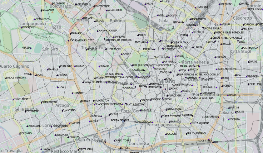
Figure 2: A fragment of the Voronoi diagram obtained from the estimated centroids of Location Areas in Milan

Abstracting from the specific dataset, telco trajectories have some important characteristics:

• Sequences of identical locations. Locations denote regions of space. Therefore, as the user’s position is matched against the closest base station, it may happen that consecutive locations are identical. For example, a phone call started and ended at home or in its proximity will generate two records reporting the same location. Notably, that does not happen in other kinds of trajectories, such as GPS and trajectories of check-in data, where consecutive locations are very unlikely identical, either for technological reasons (signal characteristics) or for the nature of movement (e.g. a check-in is typically performed once).

• CDRs are only generated when phones are actively involved in a voice call, text message or internet access. Therefore large temporal gaps exist between consecutive locations. Moreover, trajectories can contain bursts of events, often related to user’s activity on the internet (data upload and download), possibly interleaved by long periods of inactivity. The result is a highly inconsistent temporal frequency, which may confound the mobility analysis [?].

• The locations reported in CDRs can be noisy because of signal fluctuation in the network coverage [?] which can lead to ping-pong handovers between neighboring cells [?]. In addition, users can experience brief absences from the locations where they regularly stay, e.g. home. [?].

3.2 The analytical framework architecture and notation

Figure 3 displays the functional architecture of the framework. It consists of two building blocks supporting relevance and diversity analysis, respectively. In particular, given a dataset of telco trajectories, relevance analysis accomplishes two main tasks: (a) identification of key locations through trajectories summarization. The quality of clustering is assessed using internal indicators. (b) Classification of relevant locations based on frequency and attractiveness. The second building block is to characterize every single trajectory as a whole using the set of entropy-based indicators, specifically the location diversity profile and entropy rate estimation. The metrics are used for the classification of trajectories at population scale.

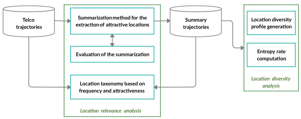
Figure 3: General architecture of the analytical framework: the datasets and the two building blocks for relevance and diversity analysis

3.3 Notation

Before proceeding, we introduce some basic notation. The dictionary $L$ indicates the set of locations, more specifically the names of the Location Areas in our dataset. Note that, throughout the paper, the terms “location” and “symbol” are used interchangeably. The discrete space of coordinated points $P$ in the Euclidean plane contains the centroids $p_{1},..,p_{n}$ of Location Areas. Thus every location has both a symbol and coordinates. The set of locations constitute the telco space.

A telco trajectory $T$ is a sequence of timestamped locations in $L$, specifying where the communication events took place. If we omit the event because irrelevant in this work, we can simply represent a telco trajectory $T$ as a symbolic trajectory: $T=(l_{1},t_{1}),..,(l_{m},t_{m})$ of length $|T|=m$ with $l_{i}\in L$. The symbols appearing in the dictionary represent (location) types, while the symbols appearing in a trajectory, (location) occurrences. We denote with $D=\{T_{1},..,T_{z}\}$, the telco dataset.

A telco trajectory typically contains multiple occurrences for the same location. For example, the weekly trajectory of an individual typically contains several occurrences of ’home’. The frequency of visit is the number of times a location appears in a trajectory. Finally, we assume that every trajectory is univocally associated with a single user. The basic notation is summarized in Table 1.

Table 1: Notation

$T,D$	Trajectory, set of trajectories
$\widehat{T},\widehat{D}$	Summary trajectory, set of summary trajectories
L, l	Location dictionary, location
$w(l,j,T),W(l,T)$	Weight of an occurrence/symbol
$\delta$	Clustering parameter: weight threshold
$N$	Clustering parameter: occurrences threshold
$H$	Shannon-Wiener diversity index
$S$	Simpson diversity index
$R$	Richness diversity index
$TD_{H}$, $TD_{S}$	Location true diversity of order 1 and 2
$S_{rate}$	Summarization rate
$Q$	Summarization goodness
$H_{r}$	Entropy rate

4 Location relevance analysis: models and methods

In this section, we describe the technique for trajectory summarization. We begin introducing a baseline technique for the lossy compression of telco trajectories based on RLE. Next, we detail our segmentation method, SeqScan-d, and present a few indicators for the evaluation of segmentation. Finally, we introduce the taxonomy proposed for location classification.

4.1 Trajectory summarization: baseline

Broadly, the operation of trajectory summarization extracts from a symbolic trajectory a series of temporally annotated locations, qualified as attractive. A first question concerns the granularity of those locations. For example, one could hypothesize that individuals commonly stay in large regions, e.g. in our case groups of nearby Location Areas, before moving to some other region. In that case, the attractive locations could be detected by applying some form of spatio-temporal segmentation (e.g. [?]), thus ignoring the symbolic dimension of locations. Actually, there is no experimental evidence that this kind of pattern exists in the reference dataset, while it is apparent that telco trajectories typically contain sub-sequences of identical symbols. This suggests an approach to segmentation based on temporal and symbolic criteria, in which attractive locations are defined at the granularity of Location Areas. The approach is presented in the following.

Baseline technique.

We start introducing a baseline technique for the extraction of attractive locations, relying on RLE compression. In general, given a sequence of values, RLE simply encodes subsequences $S$ of identical values (runs) as pairs $(l,n)$, where $l$ is the repeating value and $n\geq 1$ the count. For example, the string $aaaccvwww$ is encoded as $(a,3)(c,2)(v,1)(w,3)$.

A straightforward application of RLE to the compression of telco trajectories is as follows. Consider a trajectory $T$. Given a subsequence $S$, with repeating symbol $l$, namely $S=(l,t_{i})\ldots(l,t_{i+n-1})$, we encode $S$ as:

$$S=([t_{i},t_{i+n-1}],l,n)$$

The triple specifying the maximal time interval, the symbol and the count, i.e. $(I,l,n)$, denotes a segment of $T$. It can be seen that the replacement of a series of timestamps with a time period determines a loss of temporal information, while, by contrast, the symbolic information is naturally preserved. We refer to this compressed form as RLE-trajectory. As an example, Figure 4(a)-(b) reports a fragment of a telco trajectory and the corresponding RLE-trajectory.

We are, however, only interested in a subset of locations, those that are of major importance, therefore we slightly modify RLE-trajectories, by applying the following heuristics: we remove the segments $(I,l,n)$ where $n<N$ or $size(I)<\delta$, with $N$ and $\delta$ indicating the minimum number of communication events (i.e. symbols), and the minimum temporal extent respectively, for the segment to be meaningful. The former condition is to take into account the local frequency of communication events, the latter, the temporal irregularity of those events. We refer to the resulting trajectories as RLE+ trajectories (+ to indicate the addition of constraints). Figure 4(c) reports the portion of RLE+ trajectory obtained by compressing the native trajectory with $N=4$, $\delta=16^{\prime}$. It can be seen that the RLE+ representation consists of four segments.

Handling noise.

Unfortunately, this form of lossy compression is sensitive to noise. We call ’noise’ the unfitting symbols in a segment. Noise can result from signal fluctuations, or simply be the consequence of the user’s movement, e.g. the temporary crossing of neighbor Location Areas. The presence of noise raises two major issues: (a) it leads to a fragmented representation of summary trajectories confusing the analysis; (b) fragmentation can determine an undesirable loss of location information. We illustrate the latter case with the following example. Consider the RLE+ trajectory (fragment) in Figure 5(a). It can be seen that the user’s movement in the time period falls in three spatially adjacent Location Areas (within a touristic area) (Figure 5(b)). Yet, the segments do not satisfy the constraints (with $N=4$, $\delta=16^{\prime}$), and thus are removed from the RLE+ trajectory. As a result, the whole visit to this touristic area is removed.

Figure 4: (a) Fragment of the example trajectory (id=1470402); (b) portion of the RLE trajectory; (c) portion of the RLE+ trajectory; (d) the location found by our technique

(a)

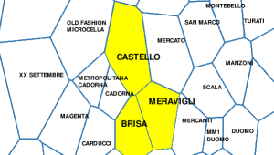
(b)

Figure 5: (a) Fragment of RLE-trajectory (Id=1470402) reporting the three adjacent locations displayed in (b). The portion of trajectory is displayed in the spatio-temporal coordinate system. The $N=4,\delta=16^{\prime}$, the RLE+ compression yields an empty sequence. Using our technique, the sequence is summarized in the location ’Castello’ (in the period from 16:35 to 18:21 of the day 24/04/2012). The location information is thus not lost

To reduce the impact of noise, we present a technique conceptually built on density-based trajectory segmentation. It requires the same parameters as RLE+, yet it allows for a more compact representation. For example, the trajectory in Figure 4(a) is summarized in one segment (see Figure 4(d)) covering the whole time of the visit. This result can be read in this way: the location (’Porta Romana’) is the most attractive location visited by the user in the period from 9:45 to 19:30 of the day 10/04/2012. Regarding the example trajectory in Figure 5(a), it can be shown that, unlike RLE+, our technique can find an attractive location (’Castello’, in the period from 16:35 to 18:21 of the day 24/04/2012), thus reducing the location information loss.

4.2 Density-based segmentation of symbolic trajectories

We propose an approach that takes inspiration from SeqScan [?]. SeqScan partitions a spatial trajectory in a series of temporally ordered clusters of arbitrary shape interleaved by sequences of unstructured points called transitions. The points that do not belong to any cluster or transition are classified as local noise. Figure 6 illustrates the concepts of cluster, transition and local noise.

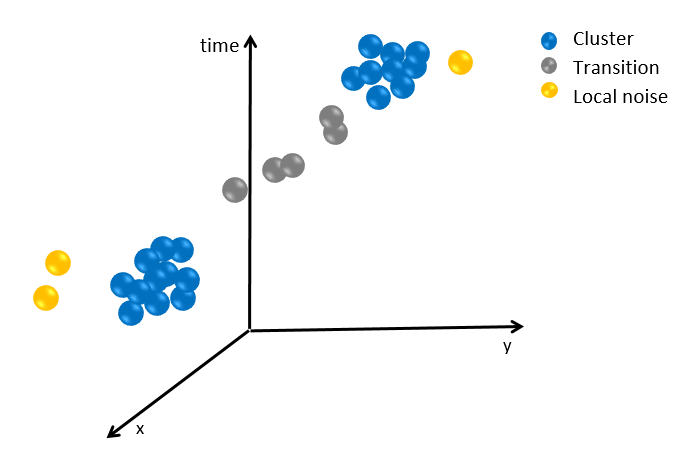
Figure 6: Density-based segmentation of a spatial trajectory [?]. The spatio-temporal points are classified as: cluster point, noise, transition point

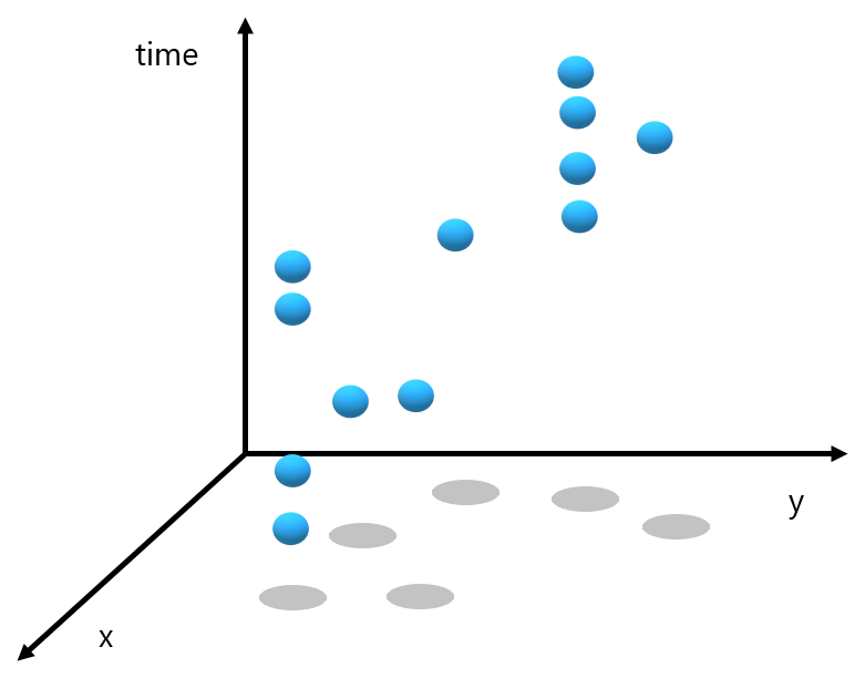
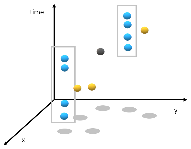
Figure 7: (a) Telco trajectory with 6 different locations (on space) and 12 occurrences (in space-time); (b) The rectangles contains two groups of occurrences for the same symbol, representing clusters along the temporal line. There are also 3 noisy points and one transition point

SeqScan is, however, tailored to spatial trajectories, while proven ineffective when applied to telco trajectories, therefore we have investigated a different strategy. To convey the intuition, consider the simple sequence in Figure 7.(a). This example shows a space of 6 locations (as points in the plane) and the trajectory of a user. It can be seen that the trajectory contains sequences of identical locations, meaning that the user is located in the same region at different times while making a phone call or accessing the Internet. As the user moves elsewhere, two cases can occur: the user returns back to the previous location; or the user starts frequenting some other location. This suggests a cluster-based segmentation performed over the temporal line with clusters only grouping occurrences of a unique location. Figure 7.(b) shows two clusters, few points of local noise and one point classified as transition. A cluster is described by a segment, i.e. a symbol and a temporal extent. Our hypothesis is that a cluster identifies the occurrence of an attractive location. We refer to this technique as SeqScan-d (discrete). Similar to RLE+, SeqScan-d requires the specification of two parameters $N$ and $\delta$. The model and the algorithm are detailed in the following.

The model

The model is built on the concept of dominant symbol. Intuitively, a dominant symbol (or location) is a symbol that is representative of a time period. The number of occurrences is a natural relevance metric. For example, in the sequence: $(a,t_{1})(a,t_{2})(b,t_{3})(a,t_{4})$, the symbol $a$ appears 3 times in the period $I=[t_{1},t_{4}]$, thus $a$ is dominant in $I$, irrespective of the presence of $b$. However, sequences can be quite complex and long, and different symbols can compete for the role. For a more selective competition, symbols are given a weight. Such weight awards temporally correlated occurrences of the same symbol. Initially every symbol has weight 0; afterwards, if two consecutive symbols at time $t_{i}$ and $t_{i+1}$ are identical, the weight of that symbol increases of a certain amount. In particular, the amount is given by the temporal distance $|t_{i+1}-t_{i}|$. A dominant location is a location that is sufficiently frequented and has high weight. More formally, consider a trajectory $T=(l_{1},t_{1})..(l_{n},t_{n})$, defined in the interval $[t_{1},t_{n}]$.

Definition 4.1 (Weight function)

We introduce:

• The function computing the weight of the occurrence of $l\in L$ at position $j$ in $T$, is defined as:

  $$w(l,j,T)=\begin{cases}|t_{j}-t_{j-1}|,&\text{ if }j>0\hbox{ and }l_{j}=l_{j-1}=l\\ 0,&\text{otherwise}.\end{cases}$$

• The weight $W(l,T)$ of a symbol $l$ over the trajectory $T$ is given by the sum of the weights of the symbol occurrences:

  $$W(l,T)=\sum_{j=1}^{n}w(l,j,T).$$ (1)

Example 1. Consider the following trajectory from $t_{1}$ to $t_{10}$ consisting of 10 occurrences, homogeneously spaced in time of 2 time units.

$$T=(a,t_{1})(a,t_{2})(c,t_{3})(a,t_{4})(c,t_{5})(b,t_{6})(b,t_{7})(a,t_{8})(b,t_{9})(b,t_{10})$$ (2)

The symbols in $T$ have the following weight:

• $W(a,T)=(t_{2}-t_{1})=2$

• $W(b,T)=(t_{7}-t_{6})+(t_{10}-t_{9})=4$

• $W(c,T)=0$

It can be seen that the symbol $b$ has the highest weight. $\diamond$

We now introduce the notion of dominant symbol. The definition is built on the auxiliary definition of well-formed sequence. Consider a sequence $T=(l_{1},t_{1})..(l_{n},t_{n})$, $N\geq 2$ and $\delta\geq 0$.

Definition 4.2 (Well-formed sequence)

We say that $T$ is a well-formed sequence if the following conditions are satisfied:

• $l_{1}=l_{n}$;

• $W(l,T)\geq\delta$;

• $|\{l_{j}\in T\mid l_{j}=l_{1}\}|\geq N$.

Condition (i) states that the sequence $S$ is bounded by $l$; (ii) and (iii) define lower bounds for the relevance measures. Now, the dominant symbol can be defined as follows:

Definition 4.3 (Dominant symbol)

Given a symbol $l$, we say that $l$ is dominant in $T$ if the following conditions are satisfied:

• $T$ is a well-formed sequence having $l$ as first symbol, i.e. $l=l_{1}$;

• Let $(l_{1},t_{1})..(l_{k},t_{k})$ the minimal-length well-formed sub-sequence of $T$ that starts at index $1$; then $(l_{k+1},t_{k+1})..(l_{n},t_{n})$, if not empty, does not contain well-formed sub-sequences having $l^{\prime}\neq l$ as first symbol.

If $l$ is dominant in $T$, the period $I=[t_{1},t_{n}]$ is called the dominance period of $l$.

The minimal-length well-formed sub-sequence at point (ii) represents the initial cluster of symbol occurrences. Such a cluster is then extended with occurrences of the same symbol and possibly noise, until a new cluster is found. As a consequence of the definition, the dominant symbol is unique in the time frame of $T$. Finally we define a summary trajectory a sequence of dominant symbols.

Definition 4.4 (Summary trajectory)

A summary trajectory $\widehat{T}$ is a trajectory of length $w$:

$$\widehat{T}=(I_{1},l_{1})..(I_{w},l_{w})$$

where the unit $(I_{j},l_{j})$ specifies the symbol $l_{j}$ dominant in the period $I_{j}$, and $I_{j}$ is maximal. The dominant symbols are the attractive locations in the native trajectory $T$.

Example 2. Consider again trajectory (2). If $N=3,\delta=2$, the summary trajectory is:

$$\widehat{T}=([t_{1},t_{4}],a)([t_{6},t_{10}],b)$$ (3)

If $N=3,\delta=4$, the summary trajectory is:

$$\widehat{T}=([t_{6},t_{10}],b)$$ (4)

Note that the summary trajectory in (4) is obtained by specifying a more restrictive temporal constraint than in (3) $\diamond$.

The condition on the maximality of the dominance period implies that the sequence is to be as long as possible, compatibly with the constraints. Summary trajectories can be straightforwardly represented using the symbolic trajectories data model in [?]. The dominant symbol identifies a cluster of occurrences, while the symbols other than the dominant symbol in a period are local noise [?] or absences in that period. Note that summarizing trajectories determines a loss of information.

The algorithm

Given the input parameters $N$ and $\delta$, the algorithm extracts a series of dominant symbols as temporally separated clusters. The symbols of the sequence are processed one at a time. As a dominant symbol is found, a cluster is created and becomes the active cluster. The algorithm proceeds trying to expand the active cluster, while monitoring at the same time the emergence of other clusters. If the active cluster is no longer expanded, and a new symbol becomes dominant, the active cluster is closed and appended to the output clusters, while a new cluster is created. The process terminates when the scan of the sequence is complete. The outcome is a series of temporally annotated clusters, each representing a dominant location.

The algorithm is detailed in Algorithm 1. The information relevant for the processing of symbols is kept in a hash table for the symbols of the telco space. For every distinct symbol $s$ of the trajectory, the tuple $(n,w,l)_{s}$ reports the number of occurrences, the weight and the index of the first occurrence in the portion of trajectory being processed. As a symbol $s$ becomes dominant, the hash table, except for the dominant symbol entry, is reset and the phase of cluster expansion starts. Upon the reading of a symbol $s^{\prime}$, two cases may occur: a) if $s^{\prime}$ is an occurrence of the dominant symbol, the entry is updated while the hash table is reset again, as above. Note that the reset operation is necessary to ensure that clusters are temporally disjointed. b) If $s^{\prime}$ is not an occurrence of the dominant symbol, the corresponding entry in the hash table is updated and the input constraints are checked. Hence, if the symbol $s^{\prime}$ becomes dominant, the current cluster is closed and the pair $(I,s)$, with $I$ denoting the time interval between the first and the last occurrence of $s$, is stored as unit of the summary trajectory. The output of the algorithm is a list of units defined over temporally separated time intervals.

The time complexity of the algorithm is linear with respect to the number of points in the original trajectory. The usage of the hash table guarantees a constant access time. As for the space requirement, the algorithm keeps in memory the original trajectory $T$, the hash table $H$ and the summary trajectory $\widehat{T}$. The size of the hash table equals the size of the dictionary $L$. Large datasets of trajectories can be summarized using modern multi-core CPUs and parallel computational frameworks. Moreover, the algorithm can be used in both batch and streaming mode.

 

Input : $T=[(l_{1},t_{1}),(l_{2},t_{2}),...]$ //trajectory

$N$, $\delta$ //input parameters

Result: $\widehat{T}$//summary trajectory

$C$=$\emptyset$ //Active cluster ;

$H$ //Hash table of $|L|$ entries ;

for $(l,t)$ in $T$ do

      

      $H$.UpdateEntry( $l$, $t$);

       if $C$=$\emptyset$ then

             if getsDominant($l$) then

                   $C$ $\leftarrow$ Cluster($l$);

                   $H$.ResetNonDominantSymbols($l$);

                  

             end if

            

      else

             if $l$==dominant($C$) then

                   $H$.ResetNonDominantSymbols($l$);

                  

            else

                   if getsDominant($l$) then

                         $\widehat{T}$.Add(close($C$));

                         $C$ $\leftarrow$ Cluster($l$);

                         $H$.ResetNonDominantSymbols($l$);

                        

                   end if

                  

             end if

            

       end if

      

end for

 

Algorithm 1 Summarization algorithm

Evaluation metrics

To evaluate the segmentation, we use two measures: summarization rate and summarization goodness, respectively, defined as follows:

• The summarization rate $S_{rate}(T)$ specifies the percentage of locations types (i.e. different symbols) in the native trajectory $T$ that do not appear in the summary trajectory $\widehat{T}$, in other words, the percentage of irrelevant locations. Let $R()$ be the number of location types in the input trajectory. We have:

  $$S_{rate}(\widehat{T})=1-\frac{R(\widehat{T})}{R(T)}$$ (5)

  $S_{rate}\approx 0$ means limited or even no summarization; $S_{rate}\approx 1$, a high level of summarization.

  Example 3. Consider the trajectory $T$, consisting of 10 occurrences, i.e. $|T|=10$ and 3 distinct location types, i.e. a, b, c:

  $$(a,t_{1})(b,t_{2})(a,t_{3})(a,t_{4})(c,t_{5})(b,t_{6})(c,t_{7})(c,t_{8})(a,t_{9})(a,t_{10})$$

  We have $R(T)=3$. Assume the following summary trajectory:

  $$\widehat{T}=([t_{1},t_{4}],a)([t_{5},t_{8}],c)([t_{9},t_{10}],a)$$

  As $\widehat{T}$ contains only 2 distinct symbols, the summarization rate is: $S_{rate}(T)=1/3$.

  Finally, we define the summarization rate $S_{rate}(\widehat{D})$ for the whole dataset as the average summarization rate of the trajectories, i.e.;

  $$S_{rate}(\widehat{D})=\frac{1}{|\widehat{D}|}\sum_{i=1}^{|\widehat{D}|}S_{rate}(\widehat{T}_{i})$$

• The goodness of a summary trajectory $Q(\widehat{T})$ measures the quality of clustering. For the evaluation of clustering, we use the internal index proposed for the validation of the SeqScan method [?] (stationary index). Accordingly, the quality of clustering is measured in terms of temporal density of clusters. In essence, the less the local noise in the period, the stronger the dominance and thus the goodness of the cluster.

  In more formal terms, let $T^{\prime}\subseteq T$ be a subsequence summarized in the unit $u_{i}=(I_{i},l_{i})$, with $l_{i}$ the dominant location in the period $I_{i}=[t_{b},t_{e}]$. We define the goodness of the unit, denoted $q(u_{i})$, as the ratio of the symbol weight in $T^{\prime}$ and the length of the dominance period, i.e., $q(u_{i})=\frac{W(l_{i},T^{\prime})}{(t_{e}-t_{b})}$. Intuitively, it can be seen as the percentage of time estimated to be spent in the dominant location. The goodness of a summary trajectory is the average goodness of the units $Q(\widehat{T})=\frac{1}{n}\sum_{i}^{n}q(u_{i})$, with $n=|\widehat{T}|$. Finally, the goodness of the summary dataset $Q(\widehat{D})$ is the average goodness of summary trajectories, i.e.:

  $$Q(\widehat{D})=\frac{1}{|\widehat{D}|}\sum_{i=1}^{|\widehat{D}|}Q(\widehat{T}_{i})$$

Example 4. Consider trajectory (2) and its summarization in two units, denoted hereinafter $u_{1},u_{2}$, i.e. $\widehat{T}=([t_{1},t_{4}],a)([t_{6},t_{10}],b)$. We have:

• $S_{rate}(T)=1/3$. In fact, there is only one irrelevant symbol, i.e. $c$.

• $Q(\widehat{T})=5/12$, where:

  • $q(u_{1})=(t_{2}-t_{1})/(t_{4}-t_{1})=1/3$

  • $q(u_{2})=[(t_{7}-t_{6})+(t_{10}-t_{9})]/(t_{10}-t_{6})=1/2$

4.3 Insights into the nature of locations: the proposal of a location taxonomy

Trajectory summarization is applied to the extraction of attractive locations from telco trajectories. We now turn to discuss the nature of the relationship between location frequency and attractiveness.

The frequency of visiting a location in fact accounts for how many times a person is there but is unable to give any information on the attractiveness that the location has on it. There may be locations, such as the bus stop, which are often visited by a person who has no specific interest in it, but just transits through it. On the contrary, we find examples such as a museum, a place that is rarely visited but that expresses a strong cultural attraction, a place therefore detected as attractive by SeqScan-d, even if visited only sporadically. The synergy between the two metrics reinforces the role that a location plays in a person’s life: locations that are both attractive and frequent are clearly very significant, while non attractive and infrequent ones are non-significant. Thus, by combining these two dimensions, we can gain further insights into the nature of the visited locations.

In particular, we distinguish four classes of locations that we label: significant (SL), transit (TL), sporadic (PL), insignificant (IL), respectively (in Figure 9). The semantics of these classes can be straightforwardly defined in set-based terms. For the sake of generality, assume a generic frequency metric. Consider a trajectory $T$ and denote with $T_{u}$ and $\widehat{T_{u}}$ the two sets of distinct locations in $T$ and $\widehat{T}$, respectively. Moreover, denote with $N_{u}$ the top-n frequented locations in $T$, where $n=|\widehat{T_{u}}|=|N_{u}|$, as shown in Figure 8. We define:

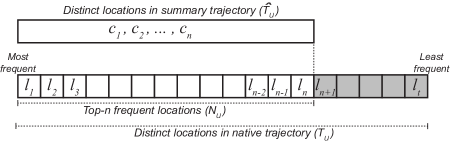
Figure 8: Schema of the sets $\widehat{T_{u}}$ and $N_{u}$ used in the relevance analysis to build the location taxonomy and to compare the frequency-based and the attractive-based approaches. Given the set $\widehat{T_{u}}$ of the $n$ attractive locations of the summary trajectory and the set $T_{u}$ of the distinct locations in the native trajectory ordered by descending frequency, the set $N_{u}$ is built by considering the top $n$-frequented locations

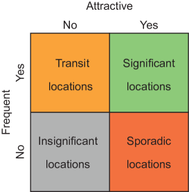
Figure 9: Location taxonomy

• Significant locations are those that are both frequent and attractive, i.e., $SL=N_{u}\cap\widehat{T_{u}}$;

• Transit locations are those that are frequent but not attractive, for example the locations where the user passes quickly daily, i.e., $TL=N_{u}\setminus\widehat{T_{u}}$;

• Sporadic locations are those that are attractive but not frequent, for example, the locations hosting some event of interest for the user, e.g., $PL=\widehat{T_{u}}\setminus N_{u}$;

• Insignificant locations are those that are neither attractive or frequent, i.e., $IL=T_{u}\setminus(\widehat{T_{u}}\cup N_{u})$.

As a result, given an input trajectory $T$ and its summarization $\widehat{T}$, we can label each distinct location in $T$, based on the proposed taxonomy. To better illustrate the operation, we use an example.

Example 5. The trajectory with ID=1470401 is summarized with parameters $N=4,\delta=16^{\prime}$. Figure 10 shows the set $T_{u}$ of locations ordered by descending frequency, the set $\widehat{T_{u}}$ of 9 locations detected by the summarization algorithm, the corresponding set of the 9 most frequent locations, i.e. $N_{u}$. The location classes $SL,TL,PL,IL$, drawn from the previous sets, are reported along with the percentage of locations for each class. It can be seen that, in this specific case, the attractive locations amount to about 12% of the total, nearly equally subdivided in significant and sporadic locations.

	Location area	Frequency
1	ABRUZZI	723
2	LAGOSTA	129
3	ACCURSIO	124
4	PORTA NUOVA	79
5	BACONE	48
6	NIGUARDA	33
7	PIOLA	23
8	MM2 CENTRALE	16
9	CARACCIOLO	16
10	STELVIO	15
11	BELGIOIOSO	12
12	VIA DE PREDIS	12
13	MARCHE	11
14	STUPARICH	10
15	MINCIO	10
16	GORINI	9
17	MORBEGNO	8
18	BUENOS AIRES PONCHIELLI	7
19	STOPPANI	7
20	PALAVOBIS	6
21	DAMIANO CHIESA	6
22	PISANI	6
23	GOBBA	6
24	GASPAROTTO	5
25	VIALE UMBRIA	5
26	LORETO	5
27	MOLINO DORINO	4
$\dots$
38	MM1 DUOMO	4
39	ROGOREDO	3
$\dots$
45	PIAZZA XXV APRILE	3
46	CASA DEL SOLE	2
$\dots$
53	MAFFUCCI	2
54	DE LELLIS	1
$\dots$
72	CONSERVATORIO	1

(a) $T_{u}$ (ordered by frequency)

	Location area
1	ABRUZZI
2	ACCURSIO
3	BELGIOIOSO
4	CHIESE
5	GORINI
6	LAGOSTA
7	MINCIO
8	NIGUARDA
9	PORTA NUOVA

(b) $\widehat{T_{u}}$

	Location area
1	ABRUZZI
2	LAGOSTA
3	ACCURSIO
4	PORTA NUOVA
5	BACONE
6	NIGUARDA
7	PIOLA
8	MM2 CENTRALE
9	CARACCIOLO

(c) $N_{u}$

	Location area
1	ABRUZZI
2	ACCURSIO
3	LAGOSTA
4	NIGUARDA
5	PORTA NUOVA

(d) $SL=N_{u}\cap\widehat{T_{u}}$

	Location area
1	PIOLA
2	MM2 CENTRALE
3	CARACCIOLO
4	BACONE

(e) $TL=N_{u}\setminus\widehat{T_{u}}$

	Location area
1	BELGIOIOSO
2	CHIESE
3	GORINI
4	MINCIO

(f) $PL=\widehat{T_{u}}\setminus N_{u}$

Transit locations	Significant locations
%TL = $\frac{|TL|}{|T_{u}|}$	%SL = $\frac{|SL|}{|T_{u}|}$
5.6%	6.9%
Insignificant locations	Sporadic locations
%IL = $\frac{|IL|}{|T_{u}|}$	%PL = $\frac{|PL|}{|T_{u}|}$
81.9%	5.6%

(g) Percentage of locations in classes

Figure 10: Partitioning of locations in classes, based on the proposed taxonomy, for the trajectory with ID=1470401. The set of insignificant locations is omitted for readability. (a) The set $T_{u}$ of distinct locations in the native trajectory ordered by frequency descending order. (b) The set $\widehat{T_{u}}$ of distinct locations in the summary trajectory. (c) The set $N_{u}$ of the top frequent locations. (d) to (f): the location taxonomy; (d) the set of locations in the significant class $SL$, (e) the set of locations in the transit class $TL$, (f) the set of locations in the sporadic class $PL$. (g) Percentage of locations in each class

5 Location diversity analysis: metrics

In this section we extend the analysis from locations to trajectories and discuss possible metrics for measuring the individual mobility, focusing in particular on entropy-based metrics. We start presenting some background on diversity indices, hence we introduce the metrics of concern.

5.1 Diversity indices

Richness, Shannon-Weiner, Simpson

We briefly overview three among the most popular diversity indices: richness, Shannon-Wiener, and Simpson. To illustrate the differences, consider an example population of 99 elements of type $a$, and 1 element of type $b$.

• Richness. Richness (R) is given by the number of types [?]. This metric does not take into account occurrences (or type abundance). Therefore, the population of the running example presents the same degree of diversity (R=2) of a population in which the elements of type $a$ and type $b$ are equally common. This index can thus yield too coarse results.

• Shannon-Wiener index. The Shannon-Wiener index is sensitive to the relative frequency of types. The index is based on the Shannon entropy:

  $$H=-\sum_{i=1}^{R}p_{i}\ln p_{i}$$

  where $p_{i}$ is the percentage of elements of type $i$, $R$ the richness (i.e. number of types), and $ln$ the natural logarithm. The entropy is maximal if types are equally common, i.e. $H_{max}=\ln{R}$, and minimal (i.e. H=0) if there is a unique type. In the previous example, the entropy is: $H\approx 0.056$.

• Simpson index. This index is defined as:

  $$S=\sum_{i=1}^{R}p_{i}^{2}$$

  It holds that $S\geq\frac{1}{R}$, with $S=1/R$ when the types are equally common. With reference to the previous example, we have $S\approx 0.98$.

True diversity

Diversity measures are hard to interpret and compare. For example, given a population $A$ with 8 equally common types and another population $B$ with 16 equally common types, the intuition is that the diversity of B is double the diversity of A. Yet, the Shannon entropy (calculated using base 2 logarithm) is 3 for $A$, and 4 for $B$. This is because entropy gives the uncertainty in type of a sample, not the number of types in the set [?]. A different approach measures the diversity in terms of Hill numbers. Proposed in the second half of the past century, Hill numbers have been recently reintroduced by biologists, e.g., [?; ?; ?]. Hill numbers are a family of diversity indices, differing among themselves only by an exponent $q$, and expressing diversity in terms of ”number of types”. The mathematical formulation is:

$$^{q}D=(\sum_{i=1}^{R}p_{i}^{q})^{\frac{1}{1-q}}$$ (6)

The measure ${}^{q}D$ is also called true diversity, while $q\geq 0$ is the diversity order. Popular diversity indices and true diversity are tightly interrelated:

• q=0: true diversity equals richness, i.e. ${}^{0}D=R$

• q=2: the true diversity is the inverse of the Simpson index, i.e.

  $${}^{2}D=1/(\sum_{i=1}^{R}p_{i}^{2})$$ (7)

• q=1: Eq. 6 is not defined, but its limit exists and equals the exponential of the Shannon-Wiener entropy:

  $${}^{1}D=\exp(-\sum_{i=1}^{R}p_{i}\ln{p_{i}})=\exp({H})$$ (8)

While we refer to the literature for further details, we highlight a few features that are relevant for our study:

• The measures of popular diversity indices can be translated into true diversity, and thus be expressed in terms of number of types. Intuitively, given the value of a diversity index, say $x$, the corresponding true diversity indicates the number of equally common types in an “equivalent” population exhibiting diversity $x$.

• The diversity order indicates the sensitivity of the diversity measure to the relative frequencies of types. In particular, the exponential of the Shannon-Wiener index (q=1) weights types by their frequency, without disproportionately favoring either rare or common types. In contrast, the inverse of the Simpson index (q=2) places more weight on the frequencies of abundant types and discounts rare types. In this sense it measures the diversity of the most popular types [?].

5.2 True location diversity and location diversity profile

We introduce the notion of true location diversity by extension. The set of locations in a summary trajectory represents the population of concern, where locations have a type and a number of occurrences. We consider the three indices: $R$, indicating the location richness; the true location diversity of order 1, based on Shannon Entropy, denoted $TD_{H}$; and the true location diversity of order 2, the inverse of the Simpson index, denoted $TD_{S}$.

Example 1. Consider two trajectories $\widehat{T}_{1}$ and $\widehat{T}_{2}$. We only report, for brevity, the series of locations forming the two trajectories, omitting the temporal information.

• $\widehat{T}_{1}=a,b,c,d,e,a,b,c,d,e,a,b,c,d,e,a,b,c,d,e,a,b,c,d,e$

• $\widehat{T}_{2}=a,b,a,b,a,b,a,c,a,b,a,b,a,b,a,d,a,b,a,c,a,b,a,e,a$

Table 2 shows the relative frequencies of the 5 locations in the two trajectories.

Table 2: Relative frequency of 5 types in $\widehat{T}_{1}$ and $\widehat{T}_{2}$

Types	$\widehat{T}_{1}$	$\widehat{T}_{2}$
a	0.2	0.52
b	0.2	0.32
c	0.2	0.08
d	0.2	0.04
e	0.2	0.04

Table 3: Diversity measures in $\widehat{T}_{1}$ and $\widehat{T}_{2}$

Measures	$\widehat{T}_{1}$	$\widehat{T}_{2}$
$R$	5	5
$TD_{H}$	5	3.2
$TD_{S}$	5	2.6

The diversity measures, homogeneously expressed in term of ’number of types’, are reported in Table 3.

It can be seen that the diversity of order $>0$ is significantly lower than $R=5$, coherently with the fact that locations are not evenly frequented. The value $TD_{H}=3.2$ measures the diversity of the typical locations in $\widehat{T}_{2}$, while $TD_{S}=2.6$, the diversity of the highly frequented locations.

Location diversity profile.

Diversity measures provide complementary information on mobility. Since all of them are relevant, we follow the approach presented by ecologists in [?], and introduce the notion of location diversity profile. The location diversity profile provides a multi-level characterization of location heterogeneity through a multiplicity of diversity indicators, globally enhancing the interpretation of the user behavior. To better illustrate the information conveyed by the diversity profile, we present an example.

Definition 5.1 (Location diversity profile)

The location diversity profile of trajectory $i$ is defined by the triple:

$$Pr(i)=(R^{i},TD_{H}^{i},TD_{S}^{i})$$ (9)

Example 2. Table 4 reports, for comparison, the Shannon entropy and the location diversity profile of four summary trajectories from the reference dataset. The Table reports two cases, discussed below:

Table 4: Shannon-Wiener entropy (H) and location diversity profile

Traj. ID	$H$	$R$	$TD_{H}$	$TD_{S}$
1595546	2.48	15	12.01	9.97
1686599	1.96	30	7.07	3.8
1477366	1.74	10	5.73	4.03
1733146	1.74	30	5.74	3.31

• (Case 1). Consider the first two trajectories $\widehat{T_{1}}$=1595546 and $\widehat{T_{2}}$=1686599. We can see that entropy $H$ is greater in $\widehat{T_{1}}$. Thus, we can infer that the uncertainty in type of a location randomly selected in $\widehat{T_{1}}$ is greater that that of a location selected in $\widehat{T_{2}}$. The diversity profile, however, provides more explicit information. In fact, we can see that $\widehat{T_{1}}$ contains fewer locations than $\widehat{T_{2}}$ (i.e. $15$ locations instead of $30$); in addition, the locations in $\widehat{T_{1}}$ are nearly all equally frequented. The second user instead, although visiting double the number of locations, frequent intensively only few locations. The behavior of the two users is thus quite different and that is also evident in the plots in Figure 11.(a)-(b), representing the summary trajectories in space and time at population scale;

• (Case 2). Consider now the last two trajectories $\widehat{T_{3}}$=1477366 and $\widehat{T_{4}}$=1733146. In this case, the value of $H$ is identical. Yet, the diversity profile shows that the two users frequent a different number of locations (i.e. $T_{3}$ reports 10 locations, $T_{4}$, 30 locations), while the number of location types in $TD_{H}$ and $TD_{S}$ is similar. The two users thus exhibit a different behavior, and that finds visual confirmation in the plots in Figure 11.(c)-(d).

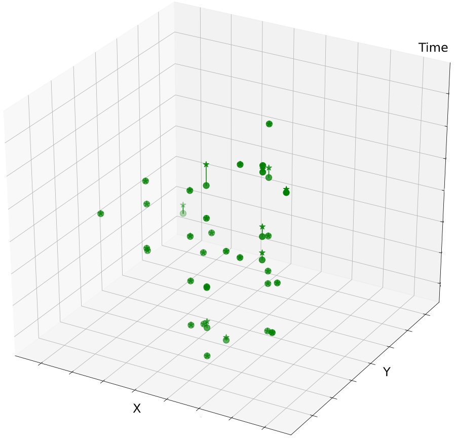
(a) ID 1595546

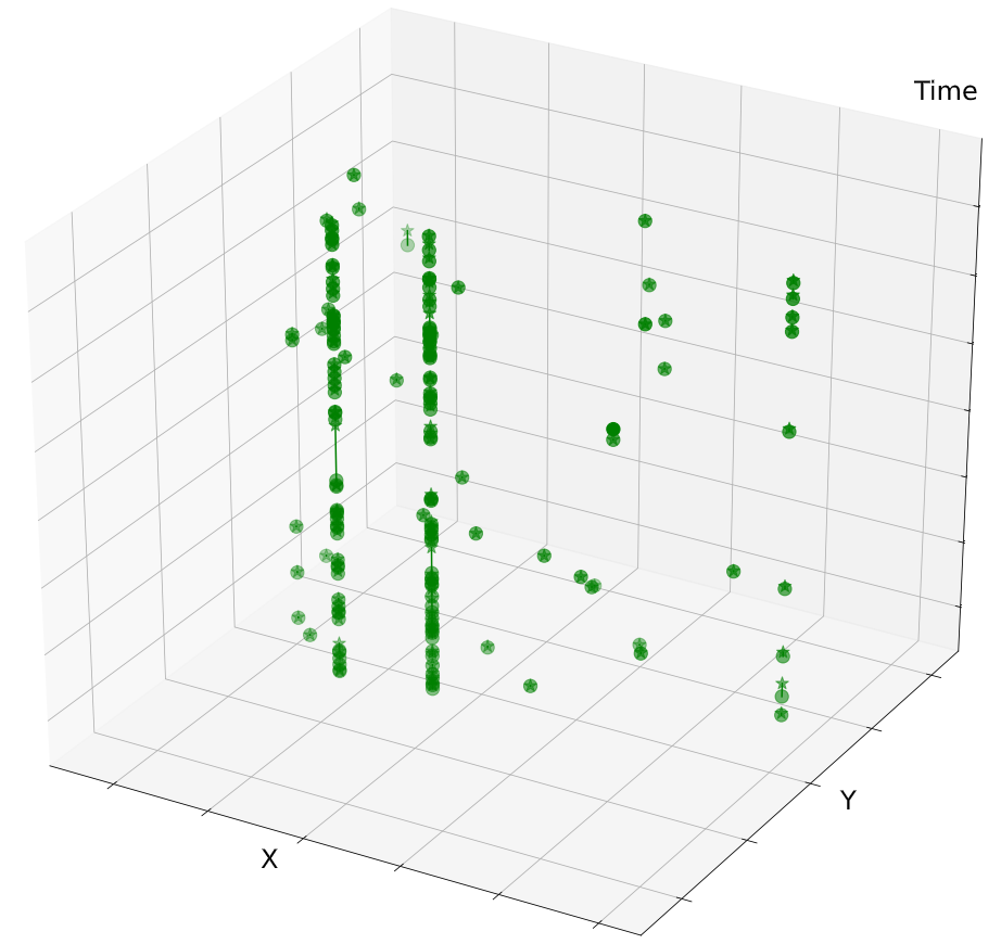
(b) ID 1686599

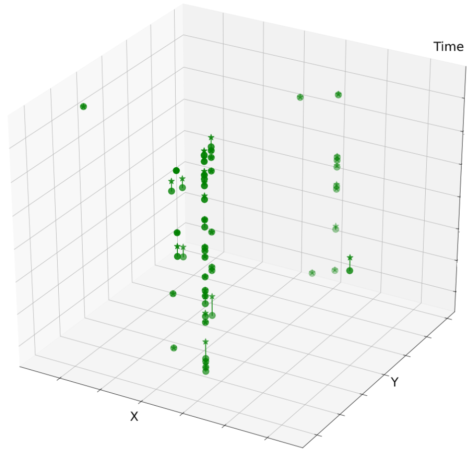
(c) ID 1477366

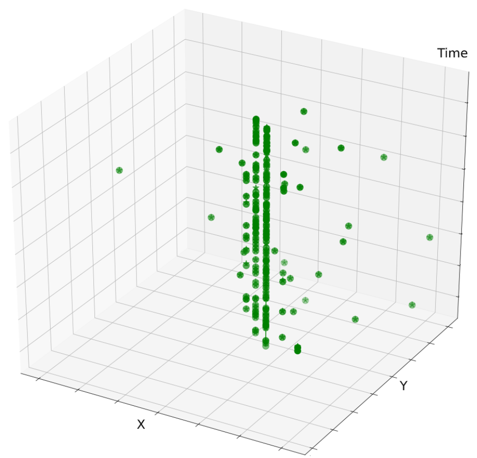
(d) ID 1733146

Figure 11: Summary trajectories represented in space (axes x,y) and time (z). The points in space are the centroids of the Location Areas

5.3 Entropy rate

The diversity indices and derived measures presented in the previous section are all based on either the number of unique visited locations or their relative frequency, so that – for example – the two trajectories

• $\widehat{T}_{1}=a,a,a,b,b,c$

• $\widehat{T}_{2}=a,b,a,c,a,b$

have the same location diversity profile. Clearly these two trajectories convey different information about the mobility of the user they refer to; in other words, intuition suggests that, in addition to the frequency of visitation, the order in which locations are visited may also be a relevant property in the assessment of the mobility behavior of an individual.

To this intent, we consider the entropy rate as another useful indicator of users’ mobility. Entropy rate is a well-known indicator and has already been used in [?] to estimate an upper bound of predictability in human mobility. In the following, we summarize its definition and propose an algorithm to estimate the entropy rate from finite sequences.

Entropy rate of stochastic processes

The content presented in this subsection is derived from [?], to which the reader is invited to refer to for a more detailed explanation.

Let $\mathcal{X}=(X_{i})_{1}^{+\infty}$ be a discrete-valued stochastic process. The entropy rate of $\mathcal{X}$ is defined as

$$H_{r}(\mathcal{X})=\lim_{n\to+\infty}\frac{1}{n}H(X_{1},X_{2},\ldots,X_{n})$$ (10)

(when the limit exists) where $H$ denotes entropy. This definition expresses the notion that entropy rate is the per-symbol entropy of the $n$ jointly distributed random variables $X_{1},X_{2},\ldots,X_{n}$.

If the process $\mathcal{X}$ is stationary (i.e. the joint distribution of any subset of random variables is invariant with respect to shifts in the index), it can be shown that $H_{r}(\mathcal{X})$ exists and equals to

$$H_{r}(\mathcal{X})=\lim_{n\to+\infty}H(X_{n}\mid X_{1},X_{2},\ldots,X_{n-1}),$$ (11)

thus expressing that, in this case, the entropy rate is the conditional entropy of the last random variable given the past.

Entropy rate estimation for finite sequences

Let $\mathbf{x}=(x_{1},x_{2},\ldots,x_{n})$ be a data realization of length $n$ drawn from the stochastic process $\mathcal{X}$. Given only $\mathbf{x}$, an exact value for the entropy rate of the originating process $\mathcal{X}$ can not be calculated, not only because we observe a merely finite-length sample of the process, so we can not compute the limit for $n\to+\infty$, but also because the joint probability distributions (of $X_{1},\ldots,X_{n}$ in (10) and of $X_{1},\ldots,X_{n-1}$ in (11)) are not known. To be able to calculate any statistical estimate, a necessary assumption is that the process is ergodic, i.e. that its statistical properties can be deduced from a sufficiently long random sample.

Several entropy rate estimators have been proposed with varying requirements, theoretical properties and performance. Here we describe the estimator defined by Theorem 1 c) in [?], derived from Lempel-Ziv compression algorithm. This estimator has a good combination of desirable properties: it is consistent (i.e. for $n\to+\infty$ it converges to the entropy rate of the process); it does not require preprocessing of data; is parameter-free; it has good performance on short sequences; is very easy to implement. The only hypothesis on $\mathcal{X}$ needed by this estimator, other than the ergodicity of the process, is the so-called Doeblin Condition, which requires that, after some number of steps, every outcome is possible again with positive probability, independently of whatever may have occurred in the past (see [?] for a formal definition).

Given a sequence $\mathbf{x}=(x_{1},x_{2},\ldots,x_{n})$ of length $n$ and the current position $i\in\{1,2,\ldots,n\}$ in the sequence, the main quantity of interest of the presented estimator is the longest match-length

$$l_{i}(\mathbf{x})=\max\left\{k\;\middle|\;\begin{aligned} &k\in\{0,\ldots,n-i+1\}\\ &(x_{i},\ldots,x_{i+k-1})=(x_{j},\ldots,x_{j+k-1})\\ &j\in\{1,\ldots,i-1\}\end{aligned}\right\},$$ (12)

that is the length of the longest subsequence starting from $i$ that has already been encountered before. The quantity

$$\widetilde{H}_{r}(\mathbf{x})=\frac{n\log_{2}(n)}{\sum_{i=1}^{n}(l_{i}(\mathbf{x})+1)}$$ (13)

is an estimator for $H_{r}(\mathcal{X})$. To compute this estimate we propose a straightforward algorithm (see Algorithm 2) having an $O(n^{3})$ worst-case complexity.

  Data: a finite sequence $(x_{1},\ldots,x_{n})$

Result: an estimate of the entropy rate of the process from which $(x_{1},\ldots,x_{n})$ is drawn

n $\leftarrow$ length ($(x_{1},\ldots,x_{n})$)

if $\textnormal{{n}}\leq 1$ then

       return $0$

end if

$\textnormal{{sum}}\leftarrow\textnormal{{n}}$

for $\textnormal{{i}}\leftarrow 2$ to n do

       l $\leftarrow$ 0

       for $\textnormal{{j}}\leftarrow 1$ to $\textnormal{{i}}-1$ do

             k $\leftarrow$ 0

             while $\textnormal{{i}}+\textnormal{{k}}\leq\textnormal{{n}}\;\&\&\;x_{\textnormal{{j}}+\textnormal{{k}}}==x_{\textnormal{{i}}+\textnormal{{k}}}$ do // $\&\&$: short-circuit AND

                   $\textnormal{{k}}\leftarrow\textnormal{{k}}+1$

             end while

            if $\textnormal{{k}}>\textnormal{{l}}$ then

                   $\textnormal{{l}}\leftarrow\textnormal{{k}}$

             end if

            

       end for

      $\textnormal{{sum}}\leftarrow\textnormal{{sum}}+\textnormal{{l}}$

end for

return $\frac{\textnormal{{n}}\log_{2}(\textnormal{{n}})}{\textnormal{{sum}}}$  

Algorithm 2 Entropy rate estimation.

Entropy rate estimation for trajectories

A summary trajectory can be considered as a finite-length sample of a discrete-valued time-correlated ergodic process; the Doeblin Condition is clearly satisfied in our application, where the history of locations visited by a user does not limit the location that they could visit in the future, so the entropy rate can be estimated from trajectories using (13).

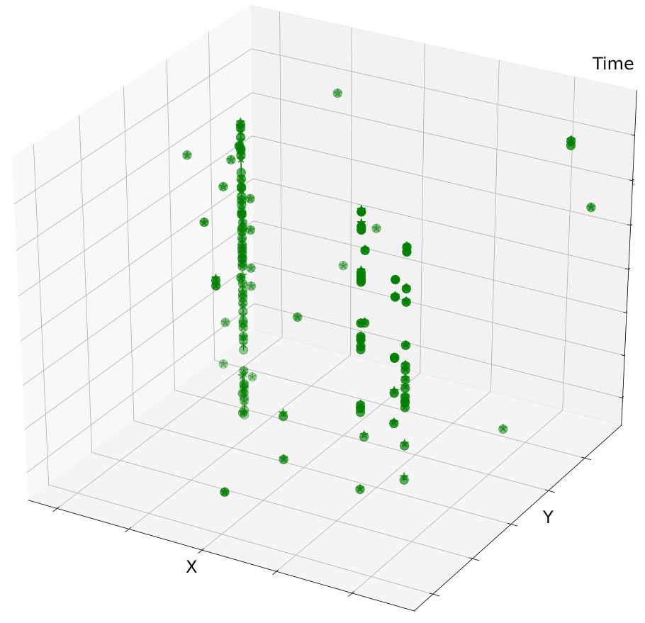
(a)

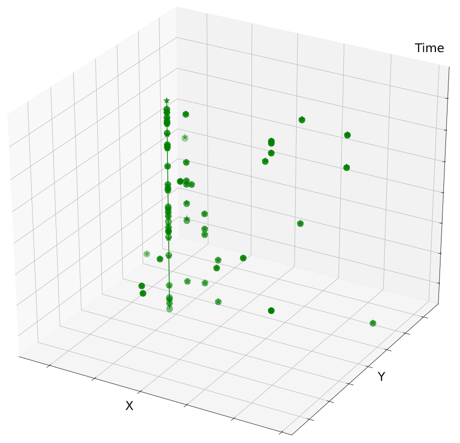
(b)

Figure 12: Summary trajectories in space and time: (a) Trajectory 1748734. (b) Trajectory 1900971. Despite having very similar location diversity profile, namely $Pr(1748734)=(16,7.34,3.88)$ and $Pr(1900971)=(16,7.31,3.87)$, the entropy rates of these two users are quite different (1.53 and 3.12 bits respectively) suggesting that their mobility behavior is different, as shown in the pictures.

Note that, since the entropy rate depends on the order of visited locations, it carries different information with respect to the indicators discussed in the previous section. Therefore the entropy rate can be useful to distinguish users who have different mobility patterns despite having the same location diversity profile. An example from the reference dataset is reported in Figure 12.

6 Experiments

We turn to evaluate the analytical framework through a series of experiments conducted on the trajectory dataset described in Section 3. The experimental activity is split into the following four tasks:

• To evaluate the SeqScan-d algorithm against the RLE-centric baseline method. The goal is to compare the summarization capabilities;

• To validate the hypothesis that attractiveness and frequency are two distinct though interrelated dimensions of location relevance. Definitely, the goal is to quantify the relation between frequent locations in native trajectories and attractive locations in summary trajectories, at population scale;

• To evaluate the utility of summary trajectories. The goal is to assess whether major statistical properties of telco trajectories reported in the literature are preserved when trajectories are summarized;

• To compute diversity measures and related metrics at population scale, and relate, where possible, those results to the literature on human mobility modeling.

In the following, we describe the experiments conducted to accomplish the above tasks. The experimental setting is defined below.

6.1 Experiment setting

Dataset.

We recall that the dataset consists of 100,000+ telco trajectories in the area of Milan, of various length and duration, over a period of 67 days. The total number of samples in the dataset amounts to about 54 million points. The telco space consists of 685 locations at the granularity of Location Area, and identified by a label. Table 5 reports the summary statistics on the number of trajectories (i.e. users), number of records, average and standard deviation of trajectory length.

Table 5: Summary statistics of the dataset

# Traj	# Records	# Loc	Avg(trj_len)	Std(trj_len)
104,413	54,193,257	685	3151	1650

Hw/sw platform.

Data summarization is performed on a Linux-Ubuntu Server DELL T620, 362 GB Ram, equipped with 2 six-cores XEON CPUs that provide 24 logic CPUs. The summarization operation is performed by partitioning the input dataset among the CPUs, and processing in parallel the smaller datasets. Data analysis is performed on a standard Windows 10 PC.

6.2 Evaluation of the summarization technique

We conduct three experiments: (a) the first is to analyze the sensitivity of summarization to the SeqScan-d parameters. This also provides the basis for the choice of the parameter configurations used in the rest of this Section. (b) The second experiment details the reduction in the number of distinct locations due to summarization. (c) The third and core experiment compares the summary trajectories generated by SeqScan-d with the set of RLE+ trajectories.

Parameter sensitivity analysis

We start running the summarization algorithm with different values for the clustering parameters $N$ and $\delta$. Table 6 reports the chosen parameters with $N$ ranging in $\{2,4,6,8\}$ and $\delta$ varying in 8 intervals from $0^{\prime}$ to $120^{\prime}$. We run the algorithm for each combination of the input values, obtaining 32 summarized datasets $\{\widehat{D}_{1},..,\widehat{D}_{32}\}$. Hence, for each summary dataset $\widehat{D}_{i}$, we compute the two performance measures, the summarization rate $S_{rate}(\widehat{D}_{i})$ and the summarization goodness $Q(\widehat{D}_{i})$.

Table 6: Input parameters for data summarization

N	$\delta(day)$
2, 4, 6, 8	0.0000 $\approx 0^{\prime}$
2, 4, 6, 8	0.0014 $\approx 2^{\prime}$
2, 4, 6, 8	0.0028 $\approx 4^{\prime}$
2, 4, 6, 8	0.0055 $\approx 8^{\prime}$
2, 4, 6, 8	0.0111 $\approx 16^{\prime}$
2, 4, 6, 8	0.0208 $\approx 30^{\prime}$
2, 4, 6, 8	0.0417 $\approx 60^{\prime}$
2, 4, 6, 8	0.0833 $\approx 120^{\prime}$

Figure 13 shows the four plots reporting the performance measures for varying values of $\delta$, and $N=2,4,6,8$. It can be seen that the goodness of summarization is generally high. For example, the plot in Figure 13(a) (for N=2) shows that, for $\delta=16^{\prime}$, the measure is 0.75. Following the experience in [?], the value of 0.7 is chosen as lower bound for a clustering of high quality. It can be also seen that the summarization rate is quite high, with the percentage of irrelevant locations (types) varying approx from 40% to 90%. In particular, with $N=2$ and $\delta=16^{\prime}$, we achieve a summarization rate of 0.74.

The parameter $N$ has a strong impact on the summarization performance. That is not surprising: the higher $N$, the longer the sequences representing clusters and thus the chance of absences in the period. Therefore, the highest goodness is achieved with $N=2$. In contrast, $\delta$ is an application-oriented parameter specifying the maximum temporal granularity of relevant locations. For example, the value $\delta=16^{\prime}$ means that the temporal extent of a cluster shall be at least 16’ (ruling out absences). For $N=2$, the two curves of the performance metrics intersect for $\delta=16^{\prime}$, which is also a reasonable value, for example, when colocated events have to be detected [?]. Thus, for $N=2$ it is convenient to set $\delta=16^{\prime}$. As $N$ increases, both $Q(D)$ and $S_{rate}(D)$ vary slightly with its variation; even, for $N=8$ they are almost constant. Based on above considerations and for the sake of readability, in the following sections we will report the results only for the four series of trajectories obtained with N=2,4,6,8 and $\delta=16^{\prime}$.

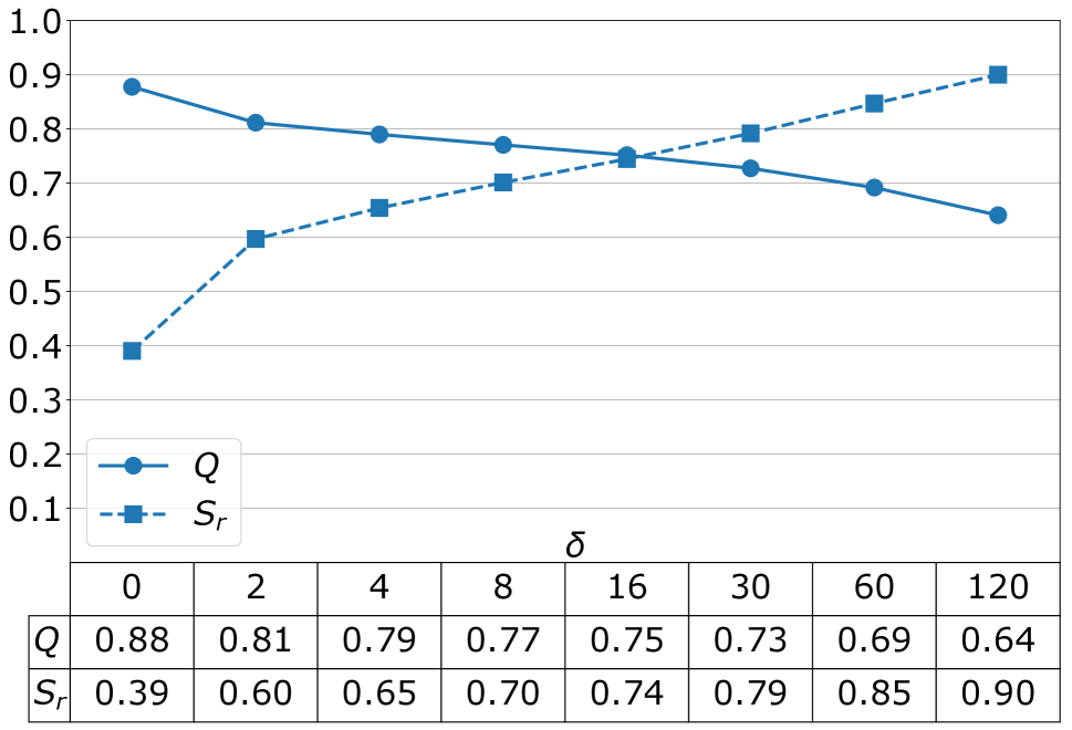
(a) $N$=2

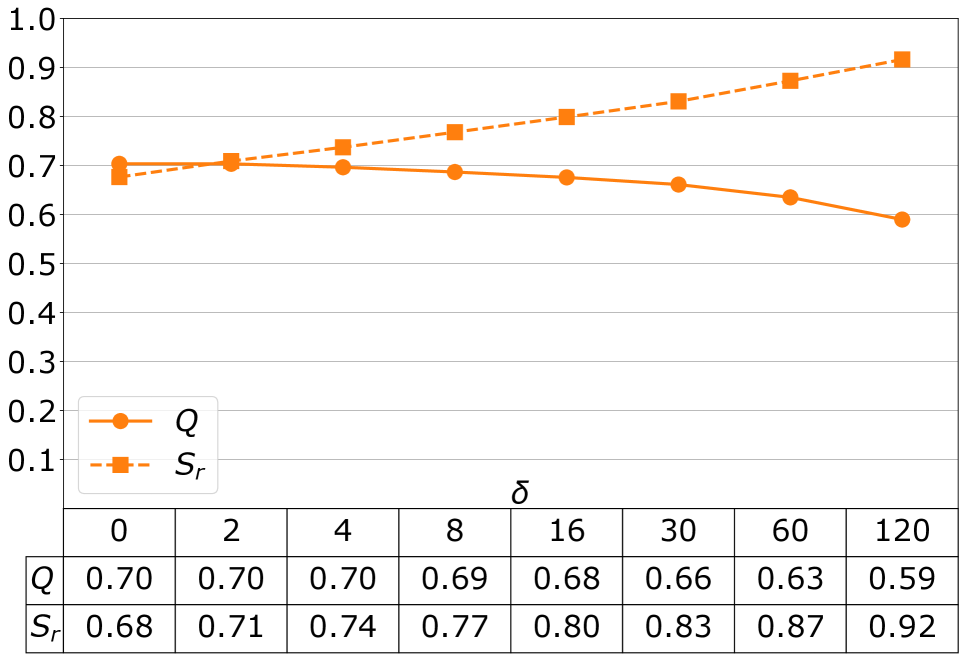
(b) $N$=4

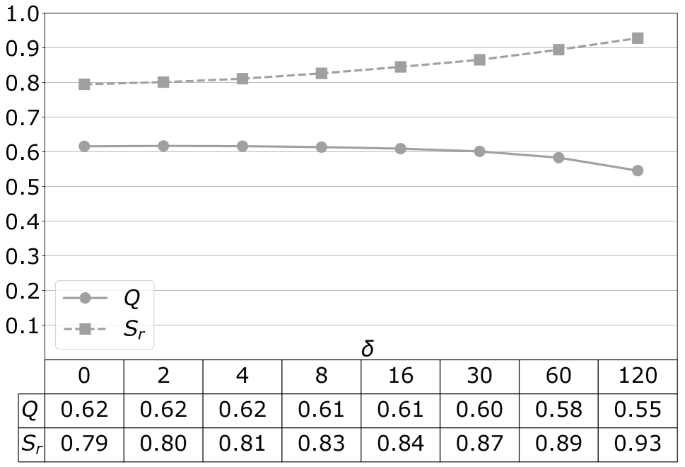
(c) $N$=6

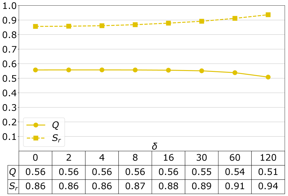
(d) $N$=8

Figure 13: The summarization goodness $Q(D)$ and the summarization rate $Sr(D)$ for $\delta$ ranging in $\{0,2,4,8,16,30,60,120\}$, and for $N$= 2, 4, 6 and 8, respectively

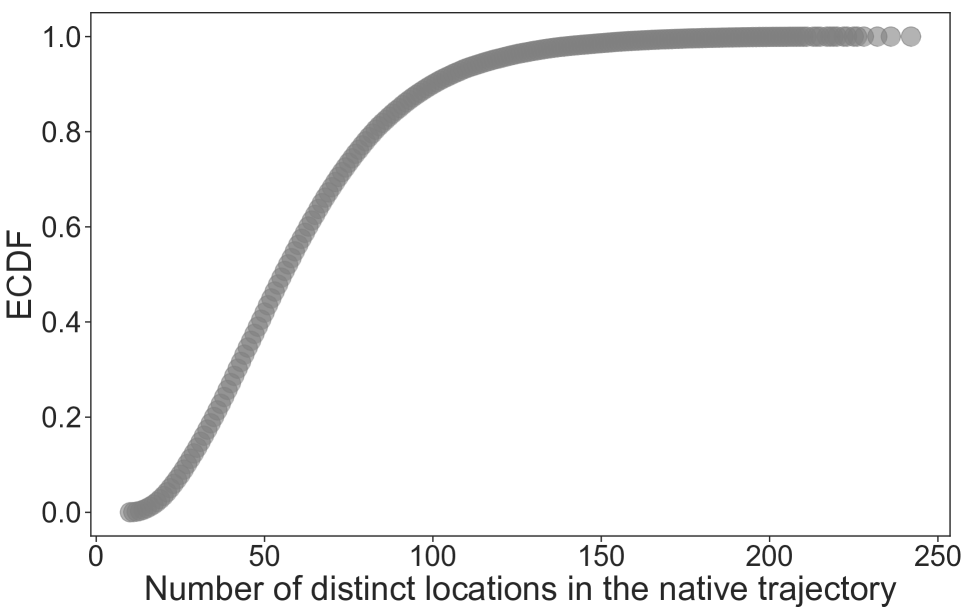
(a)

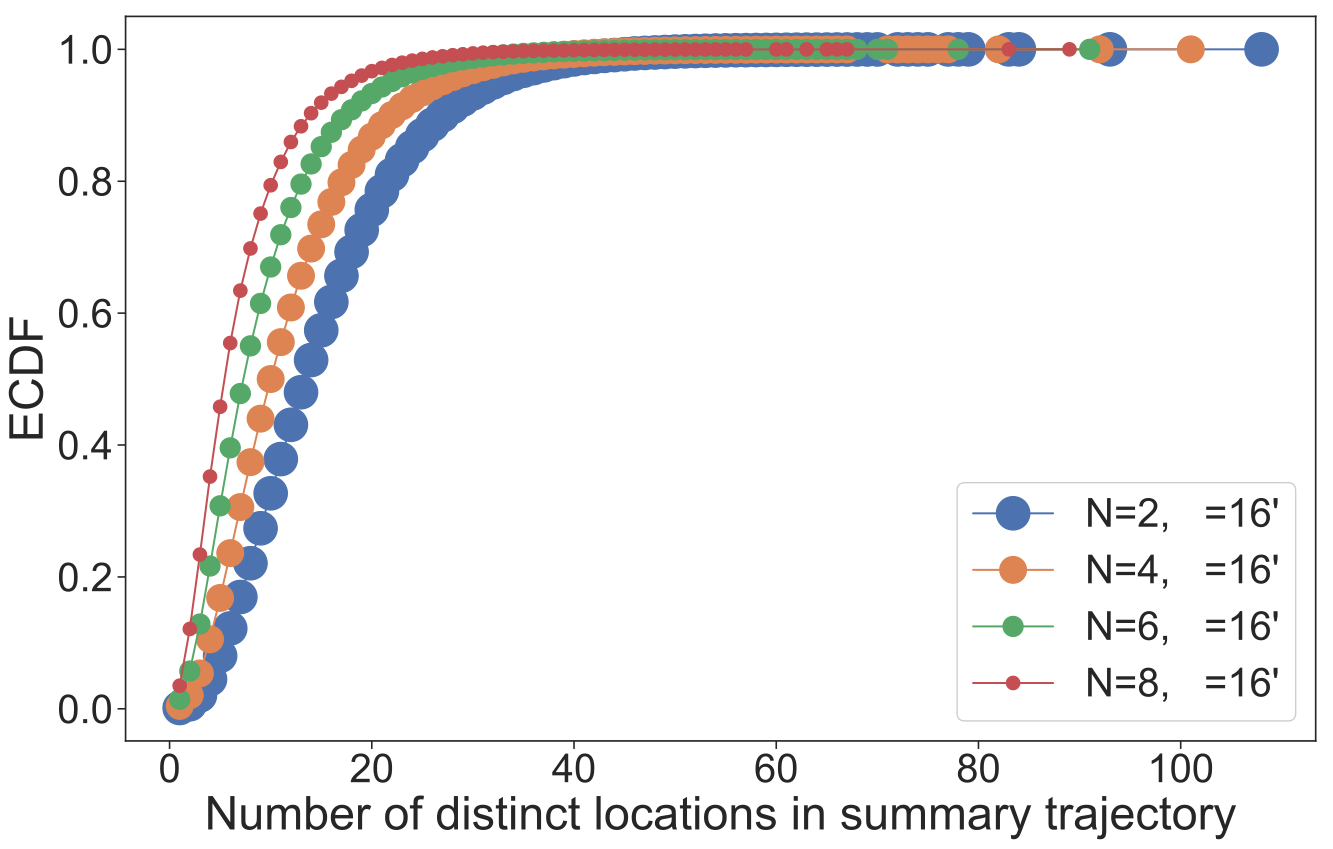
(b)

Parameters	Median	Mean	Std
Original	56.0	61.09	30.11
N=2, $\delta$=16′	14.0	15.61	8.71
N=4, $\delta$=16′	10.0	12.28	7.75
N=6, $\delta$=16′	8.0	9.47	6.59
N=8, $\delta$=16′	6.0	7.40	5.57

(c)

Figure 14: (a) Empirical Cumulative Distribution Function (ECDF) of the number of distinct locations in original trajectories. (b) ECDF of the number of distinct locations in summary trajectories. (c) Summary statistics of the number of visited distinct locations in original trajectories and in summary trajectories

Number of distinct locations in summary trajectories

This experiment provides further details on the set of locations obtained from summarization. Such a set is the basis of additional analysis that will be presented later on in the article. Figure 14 shows the distribution of the cardinality of the location sets obtained by running SeqScan-d with the aforementioned parameter configurations. As an example, for $N=4$, summary trajectories contain on average 12 distinct locations against 61 location in the original trajectories. Such locations are those that, based on our model, are attractive.

Comparison of SeqScan-d with the RLE-centric baseline technique

We compare the trajectories generated by SeqScan-d with the RLE+ trajectories. We recall that RLE+ segments denote sequences of the original trajectories reporting a unique location, thus RLE+ is sensitive to noise. We hypothesize that noise determines an excessive fragmentation of the input trajectories causing location information loss. In this experiment, we want to evaluate the impact of noise on summarization capabilities, based on the following two metrics: (a) the number of distinct locations in resulting trajectories; (b) the trajectory length, i.e. the number of segments in the trajectory. Note that we do not refer to the quality indicator $Q$ (Section 4.2), because it makes sense only for SeqScan-d and, more in general, for noise insensitive techniques.

Table 7 reports the summary statistics about the two measures computed for the reference dataset. It can be seen that:

• SeqScan-d generates shorter trajectories. For example, with $N=4,\delta=16^{\prime}$, summary trajectories are around 33% shorter than RLE+ trajectories. This result can be explained as follows: SeqScan-d not only can recognize RLE+ segments as key locations, but also is capable of aggregating RLE+ segments separated by noise, in a unique segment. The result is a reduced fragmentation.

• SeqScan-d identifies a higher number of distinct locations. For example, with the above parameters, the average number of distinct locations in summary trajectories and RLE+ trajectories is 12.28 and 11.43, respectively. In general, the set of locations types in the summary trajectories is a superset of the corresponding set in RLE+ trajectories. Thus the location information loss is lower.

Table 7: RLE+ Vs. SeqScan-d. Summary statistics of the number of distinct locations per trajectory and trajectory length

Distinct locations Trajectory length RLE+ SeqScan-d RLE+ SeqScan-d Median Mean Std Median Mean Std Median Mean Std Median Mean Std N=2 14 15.53 8.8 14 15.61 8.87 113 122.98 67.44 75 82.63 52.52 N=4 10 11.43 7.26 10 12.28 7.75 79 89.48 52.85 52 60.47 43.22 N=6 7 8.31 5.86 8 9.47 6.59 55 64.05 42.43 34 43.26 35.29 N=8 5 6.18 4.73 6 7.4 5.57 39 47.27 34.99 23 31.6 28.98

6.3 Classifying locations based on frequency and attractiveness

We conduct a first experiment to classify the location based on the taxonomy presented in Section 4.3; next we highlight an interesting property of ’significant’ locations in summary trajectories.

Given a dataset $D$, for every trajectory $T_{i}\in D$, and $\widehat{T_{i}}\in\widehat{D}$, we determine the classes of (distinct) locations labeled significant, transit, sporadic, insignificant in accordance with the definition given in Section 4.3. Let us denote the generic class as $X_{i}\in\{SL_{i},TL_{i},PL_{i},IL_{i}\}$, respectively. At population scale, the percentage of locations in class $X$ is simply computed as average:

$$X\%=\frac{1}{|D|}\sum_{i=1}^{|D|}\frac{|X_{i}|}{|T_{u_{i}}|}$$

Table 8 reports the percentages of locations in each class computed for the four datasets of summary trajectories (i.e., $N=2,4,6,8,\delta=16^{\prime}$) . It can be seen that:

• The vast majority of locations in native trajectories are classified as insignificant. The percentage varies from approx. 67% to 84%. Thus, the two approaches are in agreement that around 70% of the locations in the native trajectory are not important for the user. This result is substantially in line with the literature.

• The percentage of significant locations, i.e. frequent and attractive, computed for the whole set of locations visited by an individual varies between 9% and 19%.

• Transit (frequent but not attractive) and sporadic (infrequent but attractive) locations, together, account for 7-14%, on average, of the locations.

Table 8: Percentage of locations in native trajectories classified accordingly to the proposed taxonomy

Location class	n=2	n=4	n=6	n=8
Significant (SL)	18.67 %	14.37 %	10.96 %	8.61 %
Transit (TL)	7.13 %	5.74 %	4.43 %	3.41 %
Sporadic (PL)	7.13 %	5.74 %	4.43 %	3.41 %
Insignificant (IL)	67.05 %	74.16 %	80.17 %	84.58 %

An interesting aspect to investigate is the possible dependence of the percentage of significant locations on the number of attractive locations. Thus, we zoom in on summary trajectories, i.e. for every summary trajectory, we compute the ratio between the cardinality of the set of significant locations and the number of distinct locations in the summary trajectory. The boxplot in Figure 15 reports the percentage of significant locations in the summary trajectories, grouped by the number of distinct locations, i.e. each bar represents the distribution of the percentage of significant locations of all the trajectories with a given number of distinct locations (the value on the x-axis). It turns out that the majority of attractive locations, around $70\%$, are the most frequently visited, too. Surprisingly, we find that this result does not depend on the number of distinct locations in the summary trajectory, i.e. it holds both for people with high mobility and for more settled people visiting a limited number of locations.

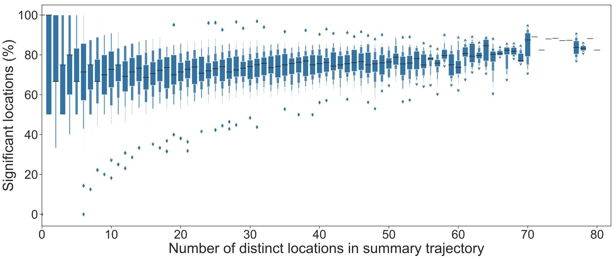
Figure 15: Boxplot of the percentage of significant locations in the summary trajectories with parameters set $N=2$, $\delta=16^{\prime}$. Each bar represents the distribution of the percentage of significant locations of all the trajectories of a given number of distinct attractive locations (the value on the x-axis)

6.4 Utility of summary trajectories

The question is whether summary trajectories preserve key statistical properties of human mobility data, that are found in literature, and, thus, data utility. We perform two experiments: (a) the first experiment is to analyze the location rank distribution in native and summary trajectories; (b) the second one is to evaluate the level of matching between the two location rankings.

Analysis of the location rank distribution

For this experiment, we refer to a key result in literature, that the frequency of visits exhibits a heavy-tail distribution, where few locations account for more than half of visiting frequencies, a limited set of locations are visited occasionally, while the long tail accounts for a large number of locations visited rarely or even once [?]. To show that this mobility dataset follows the same behavior and that the summarization algorithm does not alter the nature of this primary feature of human mobility, we follow the approach in [?], in particular, we compute the probability distribution of the location rank over the user population.

Given a generic telco dataset $D$, we define the probability $P(r,D)$ to find a user in a location with a rank $r$ as follows. For every trajectory $T\in D$, we compute the visiting frequency of every location $l\in T$ and assign $l$ a univocal rank $r$ in the range $[1,|L|]$. Hence, the probability $P(r,T)$ to find the user in the location of rank $r$, is given by the number of occurrences of the location of rank $r$, $occ(r)$, over the length of the trajectory, denoted: $P(r,T)=\frac{occ(r)}{|T|}$. Scaling up, we define the average probability $P(r,D)$ to find a user in a location of rank $r$ as:

$$P(r,D)=\frac{1}{|D|}\sum_{T_{i}\in D}{P(r,T_{i})}$$ (14)

If we compute this measure of probability over the sets $D$ and $\widehat{D}$, i.e. $P(r,D)$, $P(r,\widehat{D})$, we obtain two distributions of the location rank that can be compared.

The log-log plot of these two distributions is reported in Figure 16 for multiple choices of the two parameters of the summarization algorithm. Referring to the red curve, which provides the most different trajectory from the original one, we find that the average probability for users to be in their first relevant locations is very high and equal to 0.48 and 0.61 for $r=1$, to 0.16 and 0.21 for $r=2$, and to 0.07 and 0.09 for $r=3$ in the original and summary trajectories, respectively. We find that these values are reassuringly aligned with the literature. The discrepancies are even smaller for the other parameter settings, i.e. with $N$ decreasing, highlighting the consistency between the performance measures and the location ranking frequency. In fact, as observed in Figure 13, the lower the value of $N$, the higher the goodness of the summarization. In particular, with $N=2$ we obtain the best summarization goodness in Figure 13 and the closest curve to the original trajectories one in Figure 16 [?].

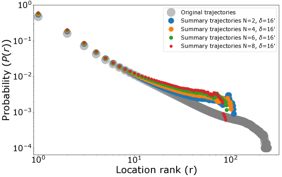
Figure 16: Plot in log-log scale of the average probability to find users in their locations as ranked by the frequency of visit. x-axis: locations ordered by descending frequency of visit and labeled by their rank. y-axis: probability to find users at a ranked location computed as the average percentage of times users were recorded in that location

Figure 16 also shows that the overall shape of the curve is not altered and the visiting probabilities are very similar in the original and summary trajectories up to around the first most visited ten locations. The summarization mainly impacts the long right tail which is shortened as the low-ranked locations are discarded by the clustering algorithm. This first result only accounts for the fact that the algorithm does not alter the probability of visiting the locations for high ranks, while eliminating the tail of visiting probabilities of low ranking locations. However, this result does not provide any evidence on the matching between the locations and their rank in the original and summarized trajectories. We can here conclude that, the summarization technique is able to preserve the frequency of the highly ranked, while discarding the locations with very low ranks. To fully affirm that the summarization technique really preserves the locations regularly frequented, while discarding the locations that are largely irrelevant to a person as they have only been there even once or may be passed through them once by chance, we will investigate the degree of matching in the following section.

Analysis of the matching degree

The problem is formulated as follows: for each trajectory, determine the maximum value $k$, such that the top-k most frequented locations in $T_{u}$, denoted $N_{u}(k)$, are also attractive, i.e. included in $\widehat{T_{u}}$.

Figure 17 reports the cumulative distribution function of the variable $k$ for different values of the parameters of the summarization algorithm.

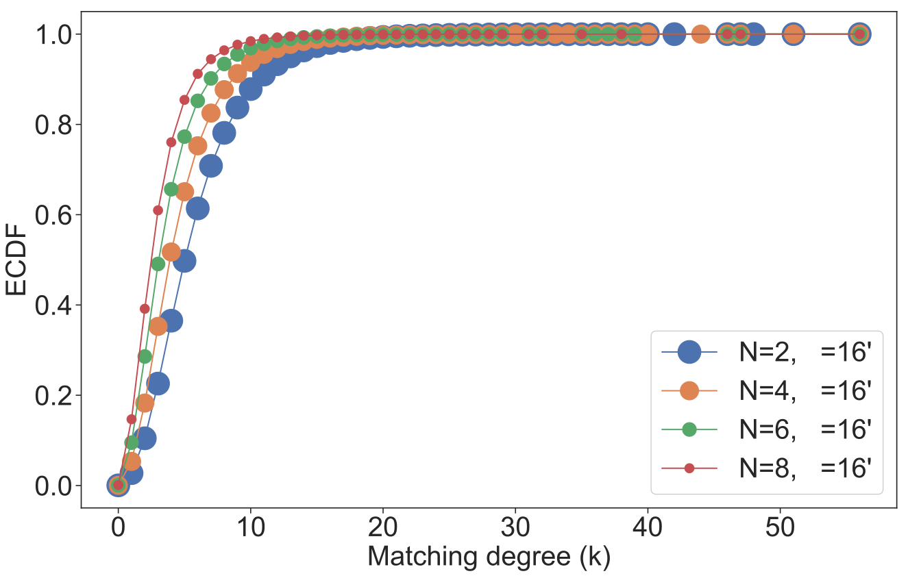
Parameters	Median	Mean	Std
N=2, $\delta$=16′	6.0	6.31	3.77
N=4, $\delta$=16′	4.0	5.10	3.20
N=6, $\delta$=16′	4.0	4.16	2.71
N=8, $\delta$=16′	3.0	3.49	2.32

Figure 17: Empirical Cumulative Distribution Function (ECDF) and summary statistics of the matching degree $k$

The value of $k$ is around 5, meaning that the summarization algorithm captures the 5 most frequently visited locations, on average. Therefore, importantly, the summarization can detect not only the routine locations as home, work and similar, but also locations which are out of the daily routine and only occasionally visited.

A related question is whether the matching degree depends on the length of the trajectory. Figure 18 plots the matching degree as function of the number of distinct locations in the summary trajectory. Interestingly, it can be seen that the matching degree $k$ tends to increase linearly with the number of attractive locations.

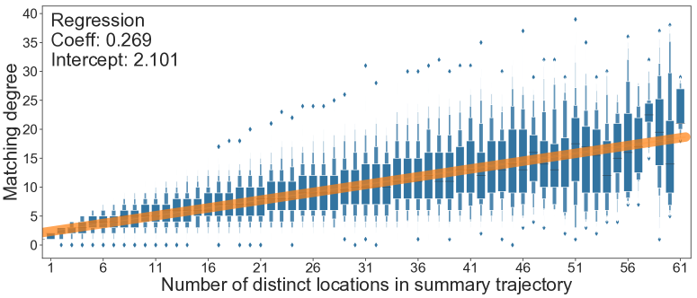
Figure 18: Boxplot of the matching degree $k$ as a function of the number of distinct locations in the summary trajectory with parameters set $N=2$, $\delta=16^{\prime}$. Each bar represents the distribution of the matching degree of all the trajectories with a given number of distinct attractive locations (the value on the x-axis). The orange line represents the linear regression of the matching degree over the number of attractive locations

6.5 Evaluating location diversity

We perform two experiments: (a) the analysis of location diversity profiles based on summary trajectories; (b) the analysis of the entropy rate.

Analysis of location diversity profiles

This experiment is organized in two steps: the first step is to compute the location diversity profile of every single trajectory; the second step is to categorize users based on location diversity indices.

Table 9: Summary statistics on the variables of the location diversity profiles.

Metric	Max	Min	Avg	Std
$R$	108	1	15.61	8.87
$TD_{H}$	91	1	6.95	3.84
$TD_{S}$	74.6	1	4.49	2.41

We consider the summarized dataset $\widehat{D}$ obtained by setting the parameters: $N=2$, $\delta=16^{\prime}$. For every trajectory $\widehat{T_{i}}\in\widehat{D}$, we compute the diversity profile: $Pr(i)=(R^{i},TD_{H}^{i},TD_{S}^{i})$. The summary statistics for the variables of the profile are reported in Table 9. It can be seen that, on average, a trajectory contains about 15 relevant locations, while the true diversity of order 1 ($TD_{H}$) amounts to about 7 locations, and the true diversity of order 2 ($TD_{S}$) to about 4 locations. There is thus a significant gap between the values of $R$ and $TD_{x}$, indicating that locations are not evenly frequented. Moreover, the diversity of core locations is quite small. Further details are provided in the next step.

User classification is performed as follows: for every variable (i.e., $R,TD_{H},TD_{S}$), we consider the sorted sequence of values (one value per trajectory). Every sequence is next partitioned in a series of 1-D clusters using the Jenks algorithm [?], finally, the relative size of every cluster is plotted as a histogram.

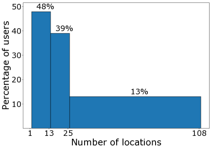
(a) Classification based on $R$

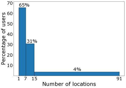
(b) Classification based on $TD_{H}$

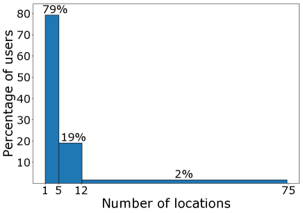
(c) Classification based on $TD_{S}$

Figure 19: User classification based on diversity indicators. The x-axis reports the number of locations, the y-axis the percentage of users

The Jenks algorithm is a data classification method that optimizes the arrangement in classes of 1D values by minimizing the within-class variance and maximizing between-class variance. As a result, the elements within each class are as close as possible in value to each other. In more detail, the algorithm splits a sequence of sorted data (unidimensional) into $k$ intervals so as to minimize the internal measure of quality, the goodness-of-variance-fit (GVF) [?]. GVF ranges between 0 and 1, with 0 indicating the worst fit and 1 the best fit. To determine a suitable value for $k$, the empirical rule is to run the algorithm for increasing value of $k$ until the GFV exceeds a threshold value. With a threshold of 0.7, we obtain $k=3$.

The plots in Figure 19 report, for each diversity measure, the three classes, i.e. low, middle and high diversity, along with the percentage of users falling in each class. Figure 19(a) shows the classification based on $R$. It can be seen that for 87% of users, the number of relevant locations is at maximum 25, while for 13% of users, it ranges between 25 and 108 locations, Figure 19(b) shows a refined classification based on $TD_{H}$: for 65% of users, the diversity of “typical location” amounts to 7 locations, while only for 4% of users the diversity is greater than 15 locations. Finally, Figure 19(c) shows the further refined classification based on $TD_{S}$. We see that, for 79% of users, the maximum diversity is 5 locations, while only for 2% of users, the diversity is greater than about 12 locations.

These results are qualitatively in line with what is reported in literature (see Section 2). We find particularly interesting the inverse of the Simpson Index, i.e. $TD_{S}$, as it provides a measure of the diversity of core locations, typically home, work, a few others. Such a measure is in line with what is known, that the great majority of people frequent assiduously only few locations.

Entropy rate at population scale

We have estimated the entropy rate of summary trajectories of the reference dataset. Summary trajectories have a rather short length (typically a few dozen symbols) and we found that the worst-case $O(n^{3})$ complexity of Algorithm 2 is not a limitation in practice, being able to estimate the entropy rate of a typical summary trajectory in about $10\,\textrm{\textmu s}$ on a standard PC. The cumulative distribution function of the entropy rate of summary trajectories of the reference dataset is shown in Figure 20. The mean value is 1.97 bits; the most complex trajectory has an entropy rate of 5.11 bits.

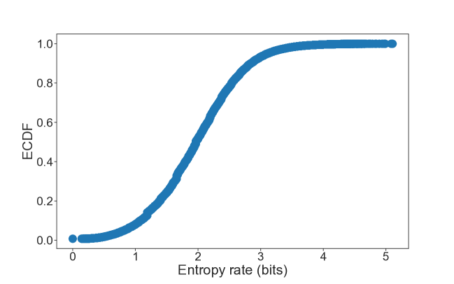
Figure 20: Empirical Cumulative Distribution Function (ECDF) of the entropy rate of summary trajectories of the reference dataset

7 Discussion

In this work, we use a research methodology that combines computational models with methods taken from human mobility modeling and ecology, for analyzing the nature of the locations frequented by individuals and thus their mobility behavior. The main findings of this effort can be summarized as follows:

• We have introduced the notion of trajectory summarization and presented the SeqScan-d algorithm for the extraction of attractive locations from symbolic trajectories with repeating symbols, in particular telco trajectories. SeqScan-d is capable of identifying key locations for each user and dispensing with the irrelevant ones, despite the high noise and uncertainty of the data. Unlike methods relying on the compression of symbolic sequences, for example based on RLE, this technique is robust against noise. That is important for the effectiveness of summarization, in that it reduces fragmentation, while preserving the semantic coherence of location visits. Concerning the parameters, the summarization goodness index is optimal with N=2. Consequently, solely the parameter $\delta$ needs to be specified, based on the applications characteristics. That streamlines the use of the operation. With the parameters $N=2$, $\delta=16^{\prime}$, the number of locations (as types) is reduced by 74% on average.

• We have devised a framework for classifying locations along the two dimensions of frequency and attractiveness. The result is a novel location taxonomy which consists of four formally defined location classes. The class of insignificant locations accounts for $67\%$ of the locations in the native trajectory with a very high concordance between the frequency-based and the attractive-based approach. The taxonomy highlights two particularly interesting classes, the transit and the sporadic locations, that on average accounts for the $14\%$ of the locations with the parameters $N=2$, $\delta=16^{\prime}$. Transit locations are for example the areas crossed by a traveler. Therefore, if a trajectory presents a high percentage of transit locations, the user is likely very mobile. Sporadic are the locations that, though important for the user, are only occasionally visited. A trajectory with many sporadic locations is typical of an individual with a non-routinary life. In synthesis, we show that the two relevance models - frequency-based and attractiveness-based - are not in contrast, but rather offer complementary viewpoints on the user behavior.

• We have shown that summary trajectories preserve the basic and universal statistical property of human mobility, that the frequency of visits follows a heavy-tail distribution, where few locations account for more than half of visiting frequencies, a limited set of locations are visited occasionally, while the long tail accounts for a large number of locations visited rarely or even once. Additionally, it is shown that the summarization operation captures the 6 most frequently visited locations, on average, with the parameters $N=2$, $\delta=16^{\prime}$ .

• We have introduced the notion of location diversity profile to capture different and multi-level facets of location diversity. This is another way for characterizing the individual mobility, this time at trajectory level and not at location level, as above. We have seen, for example, that the diversity of the locations based on the Shannon-Weiner measure amounts, on average, to seven locations (based on the exponential of the Shannon-Weiner measure), while the diversity based on the inverse Simpson index to about four locations. These results, though computed on summary trajectories, are in line with the state-of-the-art. Finally, we have introduced the entropy rate to measure entropy over sequences. Although the use of this metric for the modelling of human mobility is known, we believe it can be of broad interest also for the spatial computing community.

8 Conclusion

To summarize, in this article we have presented a location-centric framework for the analysis of the individual mobility behavior. Such analysis relies on symbolic trajectories resulting from a process of ’semantic compression’ of telco data. The code of SeqScan-d is publicly available (https://github.com/SeqScan/SeqScan-D). We have also emphasized the distinction between places of attractiveness, where users are willing to spend their time, and the locations that are frequent but not relevant where users often pass but without consuming time as those locations are not attractive to them. This distinction can be of interest in all those applications that focus on places of interest for people such as epidemics, where the identification of places where people spend time is fundamental, or recommendation systems focused on the attractiveness of places. The third and last core topic - perhaps the most challenging - regards the specification of suitable metrics for measuring the mobility behavior of individuals. This is a complex topic that requires further investigation along diverse directions, e.g. [?]. Measuring the mobility behavior can be of practical interest in many applications in which the movement of people can be naturally represented in symbolic form, such as indoor movement analysis, e.g., measuring the movement in shopping areas, museums, airports, or in urban settings. To conclude, the study of human mobility calls for a strong multidisciplinary effort to integrate data management and related application areas, e.g. urban computing, with mathematically grounded human mobility models.

References

- [1] Marta C Gonzalez, Cesar A Hidalgo, and Albert-Laszlo Barabasi. Understanding individual human mobility patterns. nature, 453(7196):779–782, 2008.
- [2] Open Geospatial Consortium. Indoorgml. http://docs.opengeospatial.org/is/14-005r5/14-005r5.html, 2018.
- [3] Dong-Wan Choi, Jian Pei, and Thomas Heinis. Efficient mining of regional movement patterns in semantic trajectories. Proceedings of the VLDB Endowment, 10(13):2073–2084, 2017.
- [4] Maria Luisa Damiani, Hamza Issa, and Francesca Cagnacci. Extracting stay regions with uncertain boundaries from gps trajectories: a case study in animal ecology. In Proc. ACM SIGSPATIAL, pages 253–262, 2014.
- [5] Hugo Barbosa, Marc Barthelemy, Gourab Ghoshal, Charlotte R James, Maxime Lenormand, Thomas Louail, Ronaldo Menezes, José J Ramasco, Filippo Simini, and Marcello Tomasini. Human mobility: Models and applications. Physics Reports, 734:1–74, 2018.
- [6] Yu Zheng, Licia Capra, Ouri Wolfson, and Hai Yang. Urban computing: concepts, methodologies, and applications. ACM Transactions on Intelligent Systems and Technology, 5(3):1–55, 2014.
- [7] Francesco Calabrese, Laura Ferrari, and Vincent D. Blondel. Urban sensing using mobile phone network data: A survey of research. ACM Comput. Surv., 47(2), November 2014.
- [8] Yu Zheng, Lizhu Zhang, Zhengxin Ma, Xing Xie, and Wei-Ying Ma. Recommending friends and locations based on individual location history. ACM Transactions on the Web, 5(1):1–44, 2011.
- [9] Jinzhong Wang, Xiangjie Kong, Feng Xia, and Lijun Sun. Urban human mobility: Data-driven modeling and prediction. SIGKDD Explor. Newsl., 21(1):1–19, May 2019.
- [10] Injong Rhee, Minsu Shin, Seongik Hong, Kyunghan Lee, Seong Joon Kim, and Song Chong. On the levy-walk nature of human mobility. IEEE/ACM transactions on networking, 19(3):630–643, 2011.
- [11] Filippo Simini, Marta C González, Amos Maritan, and Albert-László Barabási. A universal model for mobility and migration patterns. Nature, 484(7392):96–100, 2012.
- [12] Christine Parent, Stefano Spaccapietra, Chiara Renso, Gennady Andrienko, Natalia Andrienko, Vania Bogorny, Maria Luisa Damiani, Aris Gkoulalas-Divanis, Jose Macedo, Nikos Pelekis, et al. Semantic trajectories modeling and analysis. ACM Computing Surveys (CSUR), 45(4):1–32, 2013.
- [13] Boris Aronov, Anne Driemel, Marc Van Kreveld, Maarten Löffler, and Frank Staals. Segmentation of trajectories on nonmonotone criteria. ACM Trans. Algorithms, 12(2):1–28, 2015.
- [14] Maria Luisa Damiani, Fatima Hachem, Hamza Issa, Nathan Ranc, Paul Moorcroft, and Francesca Cagnacci. Cluster-based trajectory segmentation with local noise. Data Mining and Knowledge Discovery, 32(4):1017–1055, 2018.
- [15] Maria Luisa Damiani, Fatima Hachem, Christian Quadri, and Sabrina Gaito. Location relevance and diversity in symbolic trajectories with application to telco data. In Proceedings of the 16th International Symposium on Spatial and Temporal Databases, 2019.
- [16] Hancheng Cao, Jagan Sankaranarayanan, Jie Feng, Yong Li, and Hanan Samet. Understanding metropolitan crowd mobility via mobile cellular accessing data. ACM Trans. Spatial Algorithms Syst., 5(2), July 2019.
- [17] Maria Luisa Damiani and Fatima Hachem. Segmentation techniques for the summarization of individual mobility data. Wiley Interdisciplinary Reviews: Data Mining and Knowledge Discovery, 7(6):e1214, 2017.
- [18] Maike Buchin, Anne Driemel, Marc Van Kreveld, and Vera Sacristán. Segmenting trajectories: A framework and algorithms using spatiotemporal criteria. Journal of Spatial Information Science, 2011(3):33–63, 2011.
- [19] Maike Buchin, Helmut Kruckenberg, and Andrea Kölzsch. Segmenting trajectories by movement states. In Advances in spatial data handling, pages 15–25. Springer, 2013.
- [20] Andrey Tietbohl Palma, Vania Bogorny, Bart Kuijpers, and Luis Otavio Alvares. A clustering-based approach for discovering interesting places in trajectories. In Proc. ACM Symposium on Applied Computing, pages 863–868, 2008.
- [21] Zahedeh Izakian, M. Saadi Mesgari, and Robert Weibel. A feature extraction based trajectory segmentation approach based on multiple movement parameters. Engineering Applications of Artificial Intelligence, 88, 2020.
- [22] Yehezkel S Resheff. Online trajectory segmentation and summary with applications to visualization and retrieval. In 2016 IEEE International Conference on Big Data (Big Data), pages 1832–1840. IEEE, 2016.
- [23] Martin Ester, Hans-Peter Kriegel, Jörg Sander, Xiaowei Xu, et al. A density-based algorithm for discovering clusters in large spatial databases with noise. In Proc. International Conference on Knowledge Discovery and Data Mining, volume 96, pages 226–231, 1996.
- [24] Vincent D Blondel, Adeline Decuyper, and Gautier Krings. A survey of results on mobile phone datasets analysis. EPJ data science, 4(1):10, 2015.
- [25] Dirk Brockmann, Lars Hufnagel, and Theo Geisel. The scaling laws of human travel. Nature, 439(7075):462–465, 2006.
- [26] Luca Pappalardo, Filippo Simini, Salvatore Rinzivillo, Dino Pedreschi, Fosca Giannotti, and Albert-László Barabási. Returners and explorers dichotomy in human mobility. Nature communications, 6(1):1–8, 2015.
- [27] Balázs Cs Csáji, Arnaud Browet, Vincent A Traag, Jean-Charles Delvenne, Etienne Huens, Paul Van Dooren, Zbigniew Smoreda, and Vincent D Blondel. Exploring the mobility of mobile phone users. Physica A: statistical mechanics and its applications, 392(6):1459–1473, 2013.
- [28] Andrea Cuttone, Sune Lehmann, and Marta C González. Understanding predictability and exploration in human mobility. EPJ Data Science, 7(1):1–17, 2018.
- [29] Chaoming Song, Tal Koren, Pu Wang, and Albert-László Barabási. Modelling the scaling properties of human mobility. Nature Physics, 6(10):818–823, 2010.
- [30] Miao Lin, Wen-Jing Hsu, and Zhuo Qi Lee. Predictability of individuals’ mobility with high-resolution positioning data. In Proceedings of the 2012 ACM Conference on Ubiquitous Computing, UbiComp ’12, 2012.
- [31] Christian Quadri, Matteo Zignani, Sabrina Gaito, and Gian Paolo Rossi. On non-routine places in urban human mobility. In 2018 IEEE 5th International Conference on Data Science and Advanced Analytics (DSAA), pages 584–593, 2018.
- [32] Michela Papandrea, Karim Keramat Jahromi, Matteo Zignani, Sabrina Gaito, Silvia Giordano, and Gian Paolo Rossi. On the properties of human mobility. Computer Communications, 87:19 – 36, aug 2016.
- [33] Lars K Rasmussen and Ian J Oppermann. Ping-pong effects in linear parallel interference cancellation for cdma. IEEE Transactions on Wireless Communications, 2(2):357–363, 2003.
- [34] Ralf Hartmut Güting, Fabio Valdés, and Maria Luisa Damiani. Symbolic trajectories. ACM Transactions on Spatial Algorithms and Systems, 1(2):7:1–7:51, 2015.
- [35] Maria Luisa Damiani, Hamza Issa, Giuseppe Fotino, Marco Heurich, and Francesca Cagnacci. Introducing ‘presence’and ‘stationarity index’to study partial migration patterns: an application of a spatio-temporal clustering technique. International Journal of Geographical Information Science, 30(5):907–928, 2016.
- [36] Lou Jost. Entropy and diversity. Wiley Online Library Oikos, 113(2):363–375, 2006.
- [37] Hanna Tuomisto. A consistent terminology for quantifying species diversity? yes, it does exist. Oecologia, 164(4):853–60, 2010.
- [38] Anne Chao, Nicholas J. Gotelli, T. C. Hsieh, Elizabeth L. Sander, K. H. Ma, Robert K. Colwell, and Aaron M. Ellison. Rarefaction and extrapolation with hill numbers: a framework for sampling and estimation in species diversity studies. Ecological Monographs, 84(1):45–67, 2014.
- [39] Chaoming Song, Zehui Qu, Nicholas Blumm, and Albert-László Barabási. Limits of predictability in human mobility. Science, 327(5968):1018–1021, 2010.
- [40] Thomas M. Cover and Joy A. Thomas. Elements of Information Theory. Wiley, USA, 2006.
- [41] Ioannis Kontoyiannis, Paul H Algoet, Yu M Suhov, and Abraham J Wyner. Nonparametric entropy estimation for stationary processes and random fields, with applications to english text. IEEE Transactions on Information Theory, 44(3):1319–1327, 1998.
- [42] Dashun Wang, Dino Pedreschi, Chaoming Song, Fosca Giannotti, and Albert-Laszlo Barabasi. Human mobility, social ties, and link prediction. In Proceedings of the 17th ACM SIGKDD International Conference on Knowledge Discovery and Data Mining, KDD ’11, page 1100–1108, New York, NY, USA, 2011. Association for Computing Machinery.
- [43] George F Jenks. The data model concept in statistical mapping. International yearbook of cartography, 7:186–190, 1967.
- [44] Bin Jiang. Head/tail breaks: A new classification scheme for data with a heavy-tailed distribution. The Professional Geographer, 65(3):482–494, 2013.
- [45] Maria Luisa Damiani, Andrea Acquaviva, Fatima Hachem, and Matteo Rossini. Learning behavioral representations of human mobility. In Proc. ACM SIGSPATIAL, 2020.