Linear response in the uniformly heated granular gas

Abstract

We analyse the linear response properties of the uniformly heated granular gas. The intensity of the stochastic driving fixes the value of the granular temperature in the non-equilibrium steady state reached by the system. Here, we investigate two specific situations. First, we look into the “direct” relaxation of the system after a single (small) jump of the driving intensity. This study is carried out by two different methods. Not only do we linearise the evolution equations around the steady state, but also derive generalised out-of-equilibrium fluctuation-dissipation relations for the relevant response functions. Second, we investigate the behaviour of the system in a more complex experiment, specifically a Kovacs-like protocol with two jumps in the driving. The emergence of anomalous Kovacs response is explained in terms of the properties of the direct relaxation function: it is the second mode changing sign at the critical value of the inelasticity that demarcates anomalous from normal behaviour. The analytical results are compared with numerical simulations of the kinetic equation, and a good agreement is found.

I Introduction

Linear response is at the root of many important results in physics. In this respect, the fluctuation-dissipation theorem is a milestone in the development of (non-equilibrium) statistical physics [1, 2, 3]. In its original form, it relates the linear relaxation of a system to equilibrium, from an initial non-equilibrium state, with certain equilibrium time correlation functions. Very recently, this result has been extended to more general situations, which include the relaxation to non-equilibrium steady states (NESS) [4].

The above general picture makes it relevant to investigate the linear relaxation of intrinsically out-of-equilibrium systems, such as granular gases [5, 6, 7, 8], to their NESS. Due to the energy dissipation in collisions, an external energy input mechanism is needed to drive the system to a NESS. One of the simplest physical situations is that of the uniformly heated granular gas, in which all the particles of the gas are submitted to independent white noise forces of a given amplitude  [9, 10]. Therein, the granular gas remains homogeneous for all times, if it was initially so, and the main physical property of the granular gas is the granular temperature—basically, the average kinetic energy per degree of freedom. It is the amplitude of the white noise force, i.e. the intensity of this stochastic thermostat, that determines the stationary value of the granular temperature.

The main purpose of this work is to analyse the linear relaxation of the granular temperature in the uniformly heated granular gas, in several different physical situations. Due to the non-Gaussian character of the velocity distribution function, the velocity moments obey an infinite hierarchy of coupled ordinary differential equations (ODE), which must be supplemented with a closure assumption. Here, we work in the first Sonine approximation [11], in which the state of the granular system is characterised by the granular temperature $T$ and the second Sonine coefficient $a_{2}$—the excess kurtosis. The dynamics of the gas is described by a set of two ODEs for the temperature and the excess kurtosis [12], first derived in Ref. [13] for the free cooling case. These evolution equations are non-linear and have been shown to describe accurately the granular gas in many different physical situations, see for example [9, 10, 14, 15, 12, 16, 17].

First, we would like to investigate the response of the gas to an instantaneous perturbation of the driving intensity. This is a relevant problem: different memory effects have been recently reported in the uniformly heated granular gas [16, 18, 17]. In principle, the existence of these memory effect suggest that the linear relaxation of the granular temperature is non-exponential. Indeed, non-exponential relaxation [19, 20, 21, 22, 23, 24, 25] is a key ingredient for the emergence of aging and memory effects [26, 27, 28, 29, 30, 31, 32, 33, 34, 35, 36, 37] in many different physical contexts.

In light of the above, it is worth elucidating the relaxation behaviour of the granular temperature in this single-jump experiment. More specifically, we would like to clarify its exponential or non-exponential character, and also its monotonicity properties. In this respect, it is important to clarify the role played by the inelasticity. For example, a monotonic decay of the direct relaxation function ensures that the Kovacs effect is “normal”, i.e. the hump has the same sign as in molecular systems [38].

For small enough perturbations, the evolution equations for $T$ and $a_{2}$ are linearised and analytically solved. Moreover, the relaxation of both quantities to their steady values is shown to be directly related to some time correlation functions (calculated in the NESS), by extending the ideas in Ref. [4] for an out-of-equilibrium fluctuation-dissipation relation (FDR). The correlation functions involve the derivative of the $N$-particle velocity distribution function and thus we introduce a factorisation assumption—sometimes called propagation of chaos [39]—to get an explicit expression for the relevant time correlations.

Our analytical predictions are compared with Direct Simulation Monte Carlo (DSMC) results—i.e. the numerical integration of the kinetic equation. This is done for the two procedures described above. In the “direct” route, the system is initially put in the NESS corresponding to a certain value $\xi_{0}$ of the driving, the driving is instantaneously changed to $\xi$ at $t=0^{+}$, and subsequently the time evolution of the granular temperature is recorded. In the FDR route, the system is initially put in the NESS corresponding to $\xi$ and a the corresponding time correlation function is evaluated in this NESS—there is no need to change the driving.

More detailed insight into the dynamics of the system can be acquired with more complicated driving protocols. A particularly relevant one is the so-called Kovacs experiment, which has been extensively analysed in the realm of glassy systems [40, 41, 42, 43, 44, 45, 46, 47, 48, 49, 50, 51, 52]. The Kovacs protocol involves two jumps of the parameter $\xi$—temperature, driving intensity, etc.—controlling the relaxation of the system. First, it is changed from $\xi_{0}$ to $\xi_{1}<\xi_{0}$ at $t=0^{+}$ and the system relaxes towards the steady—either equilibrium or NESS—state for $\xi_{1}$. This relaxation lasts for a waiting time $t_{w}$: it is interrupted when the value of the “thermodynamic” property of interest equals the steady state value for some intermediate value of $\xi$, at $t=t_{w}^{+}$ the value of the control is changed to $\xi$ ($\xi_{1}<\xi<\xi_{0}$). If the subsequent behaviour is non-monotonic, with the thermodynamic property departing from its steady value before returning thereto, additional variables are needed to completely characterise the steady state of the system.

On the one hand, the vast majority of the studies of the Kovacs effect have been done in the non-linear regime, i.e. for large jumps of the driving, and thus the results are mainly numerical. On the other hand, a general theory of the Kovacs effect is only available within the limits of applicability of linear response theory. For molecular systems—such that the steady distribution is the canonical one—with Markovian dynamics, it has been shown that he Kovacs hump has some general characteristic features that stem from the standard version of the FDR [47]. Specifically, the Kovacs hump has only one extremum and cannot change sign, it is always normal.

In athermal systems, there appear Kovacs responses that deviate from the normal behaviour just described. The Kovacs effect is said to be anomalous when only one extremum is present but the sign of the hump changes with the system parameters. This behaviour has been observed both in the uniformly heated granular gas [16, 18] and in active matter models [53]. Also, more than one extremum has been reported in the rough granular gas [54]. It must be stressed that all these observations correspond to the non-linear regime. In particular, in the uniformly heated granular case the extreme case $\xi_{1}=0$ (i.e. no driving in the waiting time window) was considered [16, 18].

The emergence of these more complex Kovacs responses, including the anomalous behaviour, is not well understood on a general basis. Although the existence of anomalous behaviour is supported by analytical calculations in specific systems, the general physical reason behind is not known. One of the main objectives of this work is to shed light on this point by considering the linear response limit in the uniformly heated granular gas. To the best of our knowledge, the connection between the behaviour of the direct relaxation function and the Kovacs hump has not been analysed in the context of granular gases. Here, we show that the anomalous behaviour survives in linear response and thus we can explain its emergence in terms of the behaviour of the one-jump relaxation function. This is done by bringing to bear recent results on the generalisation of the mathematical structure of the linear Kovacs hump to athermal systems [53, 38].

The organisation of the paper is as follows. In Sec. II, we put forward the evolution equations for the granular temperature and the excess kurtosis and carry out their linearisation around the NESS in Sec. II.1. The linear relaxation of the granular temperature to an instantaneous change of the driving is considered in Sec. III, for different values of the inelasticity. The generalised FDR for a jump in the driving is the subject of Sec. IV. Specifically, it is derived in Sec. IV.1, and particularised for the relevant response functions in Sec. IV.2. Section V presents DSMC results for the relaxation of the granular temperature and the excess kurtosis—or, alternatively, the fourth-moment of the velocity. Next, Sec. VI is devoted to the analysis of the Kovacs experiment. Finally, conclusions and a brief discussion of perspectives for future work are presented in Sec. VII.

II Evolution equations

Let us analyse the dynamics of a granular gas of smooth hard spheres [7]. This system comprises $N$ hard particles of mass $m$ and diameter $\sigma$ in dimension $d$, which undergo inelastic collisions. In the binary collisions, the tangential component of the relative velocity remains unaltered while the normal component is reversed and shrunk by a factor $\alpha$, the normal restitution coefficient, $0\leq\alpha\leq 1$. Apart from the elastic limit $\alpha=1$, kinetic energy is lost in every collision and the undriven system “cools”, in the sense that its granular temperature—basically the average of the kinetic energy—decreases monotonically in time.

We consider the uniformly heated granular gas, i.e. the system described above is also submitted to a random forcing that inputs energy into the system. This is modelled as independent white noise forces $\bm{F}_{i}^{(p)}(t)$ acting over each grain, $\langle F_{i}^{(p)}(t)\rangle=0$ and $\langle F_{i}^{(p)}(t)F_{j}^{(q)}(t^{\prime})\rangle=m^{2}\xi^{2}\delta_{ij}\delta_{pq}\delta(t-t^{\prime})$, $i,j=1,\ldots,d$, $p,q=1,\ldots,N$. As a consequence, the system reaches a steady state in the long time limit, in which the energy input by the thermostat cancels—in average—the energy loss in collisions [9].

At the kinetic level of description, the dynamical evolution of the system is governed by the Boltzmann-Fokker-Planck equation for the velocity distribution function [9, 10]. Being the granular gas an intrinsically non-equilibrium system, its velocity distribution function is non-Gaussian, even in the steady state. The granular temperature $T(t)$ is defined as

$$\frac{d}{2}T(t)\equiv\left\langle\frac{1}{2}mv^{2}(t)\right\rangle.$$ (1)

To measure the departure from the Maxwellian distribution, the simplest approach is to consider the excess kurtosis $a_{2}$,

$$a_{2}=\frac{d}{d+2}\frac{\langle v^{4}\rangle}{\langle v^{2}\rangle^{2}}-1,$$ (2)

which vanishes for the Gaussian case. In kinetic theory, working with the pair $(T,a_{2})$ is known as the first Sonine approximation, because $a_{2}$ is the first non-zero coefficient of the expansion of the velocity distribution function in a series of Sonine polynomials [11, 9, 15, 55],

$$P_{1}(\bm{v};t)=v_{T}(t)^{-d}\pi^{-d/2}e^{-w^{2}}\left[1+a_{2}(t)S_{2}\left(w^{2}\right)\right],$$ (3)

where $\bm{w}$ is defined by

$$\bm{w}=\frac{\bm{v}}{v_{T}(t)},\qquad v_{T}^{2}(t)=\frac{2T(t)}{m}=\frac{2}{d}\langle v^{2}(t)\rangle,$$ (4)

and

$$S_{2}(x)=\frac{1}{2}x^{2}-\frac{d+2}{2}x+\frac{d(d+2)}{8}.$$ (5)

The evolution equations for the granular temperature and the excess kurtosis are derived from the Boltzmann-Fokker-Planck equation [9, 13, 15, 12, 16]. They are usually written in terms of the collision rate $\zeta_{0}$, and the stationary values of the granular temperature $T_{\text{s}}$ and the excess kurtosis $a_{2}^{\text{s}}$,

$$T_{\text{s}}=\left[\frac{m\xi^{2}}{\zeta_{0}(1+\frac{3}{16}a_{2}^{\text{s}})}\right]^{2/3},\quad\zeta_{0}=\frac{2n\sigma^{d-1}\left(1-\alpha^{2}\right)\pi^{\frac{d-1}{2}}}{\sqrt{m}d\Gamma(d/2)},$$ (6a)

$$a_{2}^{\text{s}}=\frac{16(1-\alpha)(1-2\alpha^{2})}{73+56d-24d\alpha-105\alpha+30(1-\alpha)\alpha^{2}}.$$ (6b)

By defining scaled—order of unity—variables as follows,

$$\theta=\frac{T}{T_{\text{s}}},\quad A_{2}=\frac{a_{2}}{a_{2}^{\text{s}}},\quad\uptau=\frac{\zeta_{0}\sqrt{T_{\text{s}}}}{2}t.$$ (7)

we get

$$\frac{d\theta}{d\uptau}=2\left[1-\theta^{3/2}+\frac{3}{16}a_{2}^{\text{s}}\left(1-A_{2}\theta^{3/2}\right)\right],$$ (8a)

$$\theta\frac{dA_{2}}{d\uptau}=4\left[\left(\theta^{3/2}-1\right)A_{2}+B\,\theta^{3/2}\left(1-A_{2}\right)\right],$$ (8b)

with the parameter $B$ given by 

$$B=\frac{73+8d(7-3\alpha)+15\alpha[2\alpha(1-\alpha)-7]}{16(1-\alpha)(3+2d+2\alpha^{2})}.$$ (9)

A couple of comments on the evolution equations (8) are appropriate. First, they are non-linear, so in general it is not possible to write down an analytical closed solution for them . Second, the parameters $B$ and $a_{2}^{\text{s}}$ only depend on $\alpha$ and $d$, being independent of the steady value of the temperature. In fact, all the dependence on $T_{\text{s}}$ has been incorporated into the time scale $\uptau$ introduced in Eq. (7).

It will be useful for our purposes to define the dimensionless velocity

$$\bm{c}=\frac{\bm{v}}{v_{T}^{\text{s}}},\quad v_{T}^{\text{s}}=\sqrt{\frac{2T_{\text{s}}}{m}},$$ (10)

the second moment of which is directly related to the dimensionless temperature,

$$\left\langle c^{2}\right\rangle=\frac{\left\langle v^{2}\right\rangle}{\left(v_{T}^{\text{s}}\right)^{2}}=\frac{d}{2}\theta,\qquad\left\langle c^{2}\right\rangle_{\text{s}}=\frac{d}{2}.$$ (11)

Equation (2) still holds with the change $v\to c$, whereas the fourth moment of $c$ at the steady state is given by

$$\langle c^{4}\rangle_{\text{s}}=\frac{d+2}{d}\langle c^{2}\rangle_{\text{s}}^{2}(1+a_{2}^{\text{s}})=\frac{d(d+2)}{4}(1+a_{2}^{\text{s}}).$$ (12)

II.1 Linearisation around the steady state

In this paper, we are interested in the linear relaxation of the granular gas to the steady state, in which the temperature and the excess kurtosis are $\theta_{\text{s}}=1$ and $A_{2}^{\text{s}}=1$, as a consequence of the scaling. Therefore, we write

$$\theta=1+\delta\theta,\qquad A_{2}=1+\delta A_{2},$$ (13)

insert them into Eq. (8) and neglect nonlinearities. The following linear system is thus obtained,

$$\frac{d}{dt}\delta\bm{z}=\bm{M}\cdot\delta\bm{z},$$ (14a)

$$\delta\bm{z}\equiv\begin{pmatrix}\delta\theta\\ \delta A_{2}\end{pmatrix},\qquad\bm{M}\equiv\begin{pmatrix}-3\left(1+\frac{3}{16}a_{2}^{\text{s}}\right)&-\frac{3}{8}a_{2}^{\text{s}}\\ 6&-4B\end{pmatrix}.$$ (14b)

The matrix—or operator —$\bm{M}$ does not depend on the noise intensity $\xi$ but only on the restitution coefficient $\alpha$ and the dimension $d$. This is a consequence of the rhs of the non-linear system (8) being independent of $T_{\text{s}}$, as already pointed out above.

In the following, we denote the elements of the matrix $\bm{M}$ by $M_{ij}$, i.e.

$$M_{11} =-3\left(1+\frac{3}{16}a_{2}^{\text{s}}\right), M_{12} =-\frac{3}{8}a_{2}^{\text{s}},$$

$$\ M_{21} =6, M_{22} =-4B.$$ (15)

The eigenvalues of the matrix $\bm{M}$ are both negative,

$$\lambda_{\pm}=\frac{\operatorname{Tr}\bm{M}\pm\sqrt{(\operatorname{Tr}\bm{M})^{2}-4\det\bm{M}}}{2}<0,$$ (16)

and the corresponding eigenvectors read

$$\bm{\zeta}_{+}=\begin{pmatrix}M_{12}\\ \lambda_{+}-M_{11}\end{pmatrix},\quad\bm{\zeta}_{-}=\begin{pmatrix}M_{12}\\ \lambda_{-}-M_{11}\end{pmatrix}.$$ (17)

The explicit expression for the trace and the determinant of $\bm{M}$ are

$$\operatorname{Tr}\bm{M} =-4B-3\left(1+\frac{3}{16}a_{2}^{\text{s}}\right)<0,$$ (18a)

$$\det\bm{M} =12B\left(1+\frac{3}{16}a_{2}^{\text{s}}\right)+\frac{9}{4}a_{2}^{\text{s}}>0.$$ (18b)

The general solution of the linear system is

$$\delta\bm{z}(\uptau)=C_{+}\bm{\zeta}_{+}e^{\lambda_{+}\uptau}+C_{-}\bm{\zeta}_{-}e^{\lambda_{-}\uptau},$$ (19)

or, equivalently,

$$\begin{pmatrix}\delta\theta(\uptau)\\ \delta\!A_{2}(\uptau)\end{pmatrix}\!=C_{+}\!\begin{pmatrix}M_{12}\\ \lambda_{+}\!-M_{11}\end{pmatrix}e^{\lambda_{+}\uptau}+C_{-}\!\begin{pmatrix}M_{12}\\ \lambda_{-}\!\!-M_{11}\end{pmatrix}e^{\lambda_{-}\!\uptau}.$$ (20)

The constants $C_{+}$ and $C_{-}$ are determined by the initial conditions through the relation

$$\begin{pmatrix}\delta\theta(0)\\ \delta\!A_{2}(0)\end{pmatrix}=\delta\bm{z}(0)=C_{+}\bm{\zeta}_{+}+C_{-}\bm{\zeta}_{-}.$$ (21)

III Direct relaxation after a single jump in the driving

Let us consider an experiment in which the system is initially at the steady state corresponding to some value of the driving $\xi+\delta\xi$. At the initial time, the intensity of the driving is suddenly changed from $\xi+\delta\xi$ to $\xi$: subsequently, the granular gas relaxes from its non-equilibrium steady state (NESS) at $\xi+\delta\xi$ to the corresponding NESS at $\xi$.

The initial values of the scaled variables are

$$\delta\theta(0)\neq 0,\quad\delta\!A_{2}(0)=0,$$ (22)

because the steady value of the temperature depends on the driving intensity but that of the excess kurtosis does not. Eq. (21) predicts that both $C_{+}$ and $C_{-}$ are proportional to $\delta\theta(0)$ in this case, so we write

$$C_{\pm}=\delta\theta(0)\,\tilde{C}_{\pm}$$ (23)

and readily obtain

$$\tilde{C}_{+}=\frac{M_{11}-\lambda_{-}}{M_{12}\left(\lambda_{+}-\lambda_{-}\right)},\quad\tilde{C}_{-}=\frac{\lambda_{+}-M_{11}}{M_{12}\left(\lambda_{+}-\lambda_{-}\right)}.$$ (24)

Therefore, we have that

$$\frac{\delta\bm{z}(\uptau)}{\delta\theta(0)}=\tilde{C}_{+}\bm{\zeta}_{+}e^{\lambda_{+}\uptau}+\tilde{C}_{-}\bm{\zeta}_{-}e^{\lambda_{-}\uptau}.$$ (25)

In what follows, we denote the relaxation function for the physical property $Y$ by $\phi_{Y}(\uptau)$, specifically

$$\phi_{Y}(\uptau)=\frac{\delta Y(\uptau)}{\delta\theta(0)}$$ (26)

First, we analyse the relaxation of the granular temperature, i.e.

$$\phi_{\theta}(\uptau)\equiv\frac{\delta\theta(\uptau)}{\delta\theta(0)}=a_{+}e^{\lambda_{+}\uptau}+a_{-}e^{\lambda_{-}\uptau},$$ (27)

with

$$a_{+}=\frac{M_{11}-\lambda_{-}}{\lambda_{+}-\lambda_{-}},\quad a_{-}=\frac{\lambda_{+}-M_{11}}{\lambda_{+}-\lambda_{-}}.$$ (28)

In Fig. 1, we show the two coefficients $a_{+}$ and $a_{-}$ as a function of the restitution coefficient $\alpha$, for $d=2$ and $d=3$. Both for the two and the three-dimensional case, two distinct properties are observed: (i) while $a_{+}>0$ for all values of $\alpha$, $a_{-}$ changes sign at the critical value $\alpha_{c}=1/\sqrt{2}$, specifically

$$\operatorname{sgn}(a_{-})=\operatorname{sgn}(\alpha-\alpha_{c}),\quad\alpha_{c}=1/\sqrt{2},$$ (29)

and (ii) the ratio $|a_{-}/a_{+}|\ll 1$ for all values of $\alpha$, with its larger value taking place at $\alpha=0$, for which it equals $0.0159$ ($0.0114$) for $d=2$ ($d=3$). In principle, the change of sign of $a_{-}$ at $\alpha_{c}$ might bring about a non-monotonic behaviour of the relaxation function, but this is not the case. In the long time limit, the relaxation is dominated by the largest eigenvalue $\lambda_{+}$ and, therefore,

$$\phi_{\theta}(\uptau)\sim a_{+}e^{\lambda_{+}\uptau}>0,\quad(\lambda_{+}-\lambda_{-})\uptau\gg 1.$$ (30)

Figure 1: Coefficients $a_{\pm}$ as a function of the restitution coefficient $\alpha$. Both the three-dimensional (solid line) and the two-dimensional (dashed line) are plotted. The coefficient $a_{+}$ is always positive, whereas $a_{-}$ changes sign at the critical value $\alpha=\alpha_{c}$—as given by Eq. (29). Note that $|a_{-}|$ is quite small throughout, with its least small value at $\alpha=0$, and thus $a_{+}=1-a_{-}$ is always very close to unity.

In order to understand the above behaviour of $a_{\pm}$, we bring to bear the smallness of $a_{2}^{\text{s}}$ and expand all quantities in powers of $a_{2}^{\text{s}}$. In particular, the eigenvalues $\lambda_{\pm}$ are given by

$$\lambda_{+} =-3-\frac{9(1+4B)}{16(4B-3)}a_{2}^{\text{s}}+O((a_{2}^{\text{s}})^{2}),$$ (31)

$$\lambda_{-} =-4B+\frac{9}{4(4B-3)}a_{2}^{\text{s}}+O((a_{2}^{\text{s}})^{2}).$$ (32)

Note that $4B-3>0$ ($\lambda_{+}>\lambda_{-}$). In turn, the corresponding expansion for the coefficients $a_{\pm}$ is

$$a_{+} =1+\frac{9}{4(4B-3)^{2}}a_{2}^{\text{s}}+O((a_{2}^{\text{s}})^{2}),$$ (33)

$$a_{-} =-\frac{9}{4(4B-3)^{2}}a_{2}^{\text{s}}+O((a_{2}^{\text{s}})^{2}).$$ (34)

On the one hand, it is neatly observed that $a_{-}$ is proportional to $a_{2}^{\text{s}}$, thus being rather small across the whole range of inelasticities. Moreover, the change of sign of $a_{-}$ at $\alpha_{c}$ is clearly linked to the vanishing of $a_{2}^{\text{s}}$ thereat. On the other hand, $a_{+}=1+O(a_{2}^{\text{s}})$ is very close to unity throughout, consistently with the normalisation condition $a_{+}+a_{-}=1$.

Additional information is given by the relaxation of the excess kurtosis or, equivalently, of the fourth moment $\langle c^{4}\rangle$. Eq. (25) implies

$$\phi_{\!A_{2}}(\uptau)\equiv\frac{\delta\!A_{2}(\uptau)}{\delta\theta(0)}=\frac{a_{+}a_{-}(\lambda_{+}-\lambda_{-})}{M_{12}}\left(e^{\lambda_{+}\uptau}-e^{\lambda_{-}\uptau}\right).$$ (35)

The coefficient in front of the difference of exponentials can also be expanded in powers of $a_{2}^{\text{s}}$, making use of Eqs. (II.1) and (31)–(34), with the result

$$\frac{a_{+}a_{-}(\lambda_{+}-\lambda_{-})}{M_{12}}=\frac{6}{4B-3}+\frac{27(5+4B)}{8(4B-3)^{3}}a_{2}^{\text{s}}+O((a_{2}^{\text{s}})^{2}).$$ (36)

The dominant behaviour $6/(4B-3)$ is positive for all $\alpha$: this means that $\delta A_{2}(\uptau)$ has the same sign that $\delta\theta(0)$ for all times, i.e. the same sign of $\delta\xi$ . Note that, in our experiment, the driving is instantaneously decreased from $\xi+\delta\xi$ to $\xi$ at the initial time: therefore $\delta\xi>0$ and $\delta\!A_{2}(\uptau)>0$.

The relaxation function $\phi_{\langle c^{4}\rangle}(\tau)$ can be written as a linear combination of $\phi_{\theta}$ and $\phi_{\!A_{2}}$. Bringing to bear Eqs. (2), (10) , (27), and (35), one gets

$$\delta\langle c^{4}\rangle=\frac{d(d+2)}{2}\left[\frac{1}{2}a_{2}^{\text{s}}\,\delta\!A_{2}+(1+a_{2}^{\text{s}})\delta\theta\right]$$ (37)

for the deviation of $\langle c^{4}\rangle$ from its steady state value, given by Eq. (12). The relaxation function thus reads

$$\phi_{\langle c^{4}\rangle}(\uptau)=\frac{d(d+2)}{2}\left[\frac{1}{2}a_{2}^{\text{s}}\,\phi_{\!A_{2}}(\uptau)+(1+a_{2}^{\text{s}})\phi_{\theta}(\uptau)\right].$$ (38)

IV Generalised FDR for a jump in the driving

The relaxation functions above can be related to certain time correlations in the NESS of the granular gas, by means of a generalised FDR. In the following, we first derive a generalised FDR for the relaxation of an arbitrary function of the velocities and afterwards particularise it to get the specific relations for the relaxation functions considered in the previous section.

IV.1 Derivation of the generalised FDR

Now we investigate the evolution of the granular gas, after an instantaneous jump in the driving like the one considered in the previous section. At the $N$-particle level, the fluid is described by $P_{N}(\bm{\Gamma},t)$, which is the (one-time) probability density for finding the system with $\bm{\Gamma}=(\bm{v}_{1},\bm{v}_{2},\ldots,\bm{v}_{N})$ at time $t$.

For homogeneous situations—like those considered throughout this paper, $\bm{\Gamma}$ is a Markov process described by Kac’s equation [60, 39] and for any function of the velocities we can write

$$\left\langle f(\bm{\Gamma}_{t})\right\rangle =\int d\bm{\Gamma}_{t}f(\bm{\Gamma}_{t})P_{N}(\bm{\Gamma}_{t},t)$$

$$=\int d\bm{\Gamma}_{t}\int d\bm{\Gamma}_{0}f(\bm{\Gamma}_{t})T_{t}(\bm{\Gamma}_{t}|\bm{\Gamma}_{0})P_{N}(\bm{\Gamma}_{0},0),$$ (39)

where $T_{t}(\bm{\Gamma}_{t}|\bm{\Gamma}_{0})$ is the transition probability from $\bm{\Gamma}_{0}$ to $\bm{\Gamma}_{t}$ in a time interval $t$. Thus, we have

$$P_{N}(\bm{\Gamma},t,\bm{\Gamma^{\prime}},0)=T_{t}(\bm{\Gamma}|\bm{\Gamma^{\prime}})P_{N}(\bm{\Gamma^{\prime}},0)$$ (40)

for the two-time probability density for finding the $N$-particle granular gas with $\bm{\Gamma}=(\bm{v}_{1},\bm{v}_{2},\ldots,\bm{v}_{N})$ at time $t$ and with $\bm{\Gamma^{\prime}}=(\bm{v^{\prime}}_{1},\bm{v^{\prime}}_{2},\ldots,\bm{v^{\prime}}_{N})$ at time $t=0$.

Now we consider that the initial distribution at $t=0$ corresponds to the steady state for $T(0)=T_{\text{s}}+\delta T(0)$,

$$P_{N}(\bm{\Gamma}_{0},0)\!=\!P_{N}^{\text{s}}(\bm{\Gamma}_{0})+\delta T(0)\,\frac{\partial P_{N}^{\text{s}}(\bm{\Gamma}_{0})}{\partial T_{\text{s}}}.$$ (41)

Inserting this equation into Eq. (IV.1), one gets

$$\delta\left\langle f(\bm{\Gamma}_{t})\right\rangle=\delta T(0)\int\!\!d\bm{\Gamma}_{t}\int\!\!d\bm{\Gamma}_{0}f(\bm{\Gamma}_{t})T(\bm{\Gamma}_{t}|\bm{\Gamma}_{0})\frac{\partial P_{N}^{\text{s}}(\bm{\Gamma}_{0})}{\partial T_{\text{s}}},$$ (42)

in which we have defined, consistently with the notation we employ throughout,

$$\delta\left\langle f(\bm{\Gamma}_{t})\right\rangle\equiv\left\langle f(\bm{\Gamma}_{t})\right\rangle-\left\langle f(\bm{\Gamma})\right\rangle_{\text{s}}$$ (43)

for the deviation of the average value of $f$ from its steady state value.

Equation (42) can be rewritten as

$$\delta\left\langle f(\bm{\Gamma}_{t})\right\rangle=\delta T(0)\left\langle f(\bm{\Gamma}_{t})\frac{\partial\ln\!P_{N}^{\text{s}}(\bm{\Gamma}_{0})}{\partial T_{\text{s}}}\right\rangle_{\!\!\text{s}},$$ (44)

there emerges the time correlation function

$$C_{\!f}(t)\equiv\left\langle f(\bm{\Gamma}_{t})\frac{\partial\ln\!P_{N}^{\text{s}}(\bm{\Gamma}_{0})}{\partial T_{\text{s}}}\right\rangle_{\!\!\text{s}}$$

$$\;\;=\int\!\!d\bm{\Gamma}_{t}\int\!\!d\bm{\Gamma}_{0}f(\bm{\Gamma}_{t})\frac{\partial\ln\!P_{N}^{\text{s}}(\bm{\Gamma}_{0})}{\partial T_{\text{s}}}T(\bm{\Gamma}_{t}|\bm{\Gamma}_{0})P_{N}^{\text{s}}(\bm{\Gamma}_{0}).$$ (45)

Therefore, we can also obtain the relaxation functions by measuring correlations at the NESS, which is the expression of the generalised FDR. The subindex $s$ in $\left\langle\cdots\right\rangle_{\text{s}}$ stresses that the average in the time correlation function is done in the steady state, because

$$T(\bm{\Gamma}_{t}|\bm{\Gamma}_{0})P_{N}^{\text{s}}(\bm{\Gamma}_{0})=P_{N}^{\text{s}}(\bm{\Gamma}_{t},t,\bm{\Gamma}_{0},0)$$ (46)

is the two-time probability density at the steady state with temperature $T_{\text{s}}$ .

The difficulty of this approach is the necessity of knowing the $N$-particle distribution $P_{N}^{\text{s}}(\bm{\Gamma}_{0})$: note that one deals with the one-particle distribution function in the kinetic approach. This difficulty is usually circumvented by introducing the following factorisation ansatz [4]

$$P_{N}^{\text{s}}(\bm{\Gamma})=\prod_{i=1}^{N}P_{1}(\bm{v}_{i}),$$ (47)

which is sometimes called “propagation of chaos” [39]. This is more restrictive than the usual molecular chaos hypothesis employed to derive the Boltzmann equation: therein, only the two-particle distribution is assumed to factorise. With the assumption (47), $C_{\!f}(t)$ simplifies to

$$C_{\!f}(t)=\sum_{i=1}^{N}C_{\!f}^{i}(t),\quad C_{\!f}^{i}(t)\equiv\left\langle f(\bm{\Gamma}_{t})\frac{\partial\ln\!P_{1}^{\text{s}}(\bm{v}_{i0})}{\partial T_{\text{s}}}\right\rangle_{\!\!\text{s}},$$ (48)

where $P_{1}^{\text{s}}$ is the stationary solution of the Boltzmann equation, which is—at least approximately—known.

IV.2 Response functions

Here, we derive the specific formulas relating the relaxation functions $\phi_{\theta}$ and $\phi_{\langle c^{4}\rangle}$ to time correlations. To achieve this goal, we need $\partial_{T_{\text{s}}}\ln\!P_{N}^{\text{s}}(\bm{\Gamma})$ and thus we use the propagation of chaos assumption (47). Consistently with our approach, we employ the one-particle velocity distribution function in the first Sonine approximation. Particularising (3) to the steady state, we have

$$P_{1}^{\text{s}}(\bm{v})=\left(v_{T}^{\text{s}}\right)^{-d}e^{-c^{2}}\left[1+a_{2}^{\text{s}}S_{2}\left(c^{2}\right)\right],$$ (49)

where $\bm{c}$ is defined in Eq. (10). Taking into account that $\partial c^{2}/\partial T_{\text{s}}=-c^{2}/T_{\text{s}}$, we get

$$\frac{\partial\!\ln\!P_{1}(\bm{v})}{\partial T_{\text{s}}}=-\frac{d}{2T_{\text{s}}}+\frac{1}{T_{\text{s}}}c^{2}-\frac{1}{T_{\text{s}}}c^{2}\frac{a_{2}^{\text{s}}S_{2}^{\prime}\left(c^{2}\right)}{1+a_{2}^{\text{s}}S_{2}\left(c^{2}\right)}.$$ (50)

By defining

$$g(x)=-\frac{d}{2}+x-x\frac{a_{2}^{\text{s}}S_{2}^{\prime}(x)}{1+a_{2}^{\text{s}}S_{2}(x)},$$ (51)

we can write

$$\frac{\partial\!\ln\!P_{1}(\bm{v})}{\partial T_{\text{s}}}=\frac{1}{T_{\text{s}}}g\!\left(c^{2}\right),\quad C_{f}^{i}(t)=\frac{1}{T_{\text{s}}}\left\langle f(\bm{\Gamma}_{t})\,g\!\left(c_{i0}^{2}\right)\right\rangle_{\text{s}}.$$ (52)

and thus the response function is given by

$$\delta\left\langle f(\bm{\Gamma}_{t})\right\rangle=\delta\theta(0)\sum_{i=1}^{N}\left\langle f(\bm{\Gamma}_{t})\,g\!\left(c_{i0}^{2}\right)\right\rangle_{\text{s}}.$$ (53)

Now we particularise the above general relation to the specific cases we are interested in. Note that the dimensionless time $\uptau$ is then used, instead of $t$. First, we consider the following choice for the function $f$,

$$f(\bm{\Gamma}_{\uptau})=\frac{1}{N}\sum_{i=1}^{N}\left(\frac{2}{d}c_{i}^{2}(\uptau)-1\right),\quad\left\langle f(\bm{\Gamma}_{\uptau})\right\rangle=\delta\theta(\uptau).$$ (54)

Making use of Eq. (53), we have for the relaxation function of the granular temperature

$$\phi_{\theta}(\uptau)=R_{2}(\uptau)\equiv\frac{1}{N}\sum_{i=1}^{N}\sum_{j=1}^{N}\left\langle\left(\frac{2}{d}c_{i}^{2}(\uptau)-1\right)g(c_{j}^{2}(0))\right\rangle_{\!\!\text{s}}.$$ (55)

Second, we consider the relaxation of the fourth moment. Therefore, now we choose $f$ to be

$$f(\bm{\Gamma}_{\uptau})=\frac{1}{N}\sum_{i=1}^{N}\left(c_{i}^{4}(\uptau)-\left\langle c^{4}\right\rangle_{\text{s}}\right),\quad\left\langle f(\bm{\Gamma}_{\uptau})\right\rangle=\delta\left\langle c^{4}(\uptau)\right\rangle,$$ (56)

where $\left\langle c^{4}\right\rangle_{\text{s}}$ is given by Eq. (12). Again, we employ (53) to write

$$\phi_{\left\langle c^{4}\right\rangle}(\uptau)=R_{4}(\uptau)\equiv\frac{1}{N}\sum_{i=1}^{N}\sum_{j=1}^{N}\left\langle\left(c_{i}^{4}(\uptau)-\left\langle c^{4}\right\rangle_{\text{s}}\right)g(c_{j}^{2}(0))\right\rangle_{\text{s}}$$ (57)

V Numerical simulations

Now we compare our analytical predictions for the relaxation function with numerical data obtained from the DSMC numerical integration of the Boltzmann-Fokker-Planck equation. We have employed a system of $N=10^{6}$ hard discs ($d=2$) of unit mass $m=1$ and unit diameter $\sigma=1$, with the binary collision rule between particles $i$ and $j$

$$\bm{v}_{i}^{\prime}=\bm{v}_{i}-\frac{1+\alpha}{2}(\bm{\hat{\sigma}}\cdot\bm{v}_{ij})\bm{\hat{\sigma}},\quad\bm{v}_{j}^{\prime}=\bm{v}_{j}+\frac{1+\alpha}{2}(\bm{\hat{\sigma}}\cdot\bm{v}_{ij})\bm{\hat{\sigma}}.$$ (58)

Above, $(\bm{v}_{i},\bm{v}_{j})$ are the precollisional velocities, $(\bm{v}_{i}^{\prime},\bm{v}_{j}^{\prime})$ are the post-collisional ones, $\bm{v}_{ij}\equiv\bm{v}_{i}-\bm{v}_{j}$ is the relative velocity and $\bm{\hat{\sigma}}$ is the unit vector pointing from the centre of particle $j$ to the centre of particle $i$ at the collision. Moreover, in order to simulate the stochastic thermostat, the hard discs are submitted to random kicks every $N_{c}=500$ collisions. In the kick, each component of the velocity of every particle is incremented by a random number extracted from a Gaussian distribution of variance $\xi^{2}\Delta t$, where $\Delta t$ is the time interval corresponding to the number of collisions $N_{c}$.

V.1 Relaxation function of the temperature

In particular, we show the relaxation functions corresponding to $\alpha=0.3$ ($>\alpha_{c}$), $\alpha=0.7$ ($\simeq\alpha_{c}$), and $\alpha=0.9$ ($<\alpha_{c}$)—see panels (a) to (c) of Fig. 2. The symbols represent simulation results from a NESS at $(\xi+\delta\xi)^{2}=0.205$ to the NESS corresponding at $\xi^{2}=0.2$, while the solid lines represent our theoretical prediction (27). The agreement is excellent, which comes as no surprise because the first Sonine approximation is known to give a good description of the granular gas dynamics—although the majority of the studies have been done in the non-linear regime [12, 16, 18].

Figure 2: Relaxation function of the granular temperature as a function of the scaled time $\uptau$. Panels (a), (b), and (c) display $\phi_{\theta}(\uptau)$ for three different values of the restitution coefficient, namely $\alpha=0.3$, $\alpha=0.7$ and $\alpha=0.9$, respectively—symbols correspond to simulation results in a system of $10^{6}$ particles averaged over $10$ runs, and lines to the analytical prediction (27). The three simulation curves are plotted together in panel (d), where it is clearly seen that they superimpose. Therefore, the linear relaxation of the granular temperature to the corresponding NESS is “universal” in the $\uptau$ scale.

In principle, Eq. (27) tells us that the relaxation of the granular temperature to the NESS is non-exponential. However, the smallness of the coefficient $a_{-}$ throughout the whole $\alpha$ range entails that, from a practical point of view, the relaxation is very well fitted by a single exponential for all values of the restitution coefficient. Moreover, the relaxation functions for different values of $\alpha$ superimpose, when plotted as a function of the scaled time $\uptau$ . This is neatly observed in panel (d) of Fig. 2, where we have put together the simulation results from the three previous panels. This stems from the weak $\alpha$-dependence of the eigenvalue $\lambda_{+}$, which is close to $-3$ for all values of $\alpha$, as predicted by Eq. (31) and shown in panel (a) of Fig. 3. Therein, it is observed that the maximum deviation from $-3$ is of the order of $3\%$, for the largest value of $a_{2}^{\text{s}}$—i.e. in the completely inelastic limit $\alpha=0$. For completeness, we show $\lambda_{-}$ in panel (b) of the same figure.

Figure 3: Relaxation rates $\lambda_{\pm}$ as a function of the restitution coefficient. Again, both $d=3$ (solid line) and $d=2$ (dashed) are plotted. The largest rate $\lambda_{+}$ is always close to $-3$ throughout. The smaller rate $\lambda_{-}$ has a stronger dependence on $\alpha$, diverging in the elastic limit $\alpha\to 1^{-}$.

Now we proceed to evaluate the relaxation function of the temperature by using the FDR relation (55). The correlation function on the rhs has been numerically evaluated from the DSMC data, employing system with $N=10^{4}$–$10^{6}$ hard discs and averaging over a long trajectory of duration $\Delta\uptau=400$–$6000$, depending on the value of $\alpha$. We compare the numerics with Eq. (55) for $\phi_{\theta}$ in Fig. 4. On the one hand, we observe in the left panel that there appears a discrepancy at the initial time. The value stemming from the FDR relation deviates from unity in general: it is larger (smaller) for $\alpha=0.3$ $\alpha=0.9$, whereas it equals one for $\alpha=0.7\simeq\alpha_{c}$. On the other hand, the right panel shows that this discrepancy disappears if we normalise the correlation function $R_{2}(\uptau)$ with its initial value, i.e. if we compare $\phi_{\theta}(\uptau)$ with $R_{2}(\uptau)/R_{2}(0)$. Therefore, the correlation $R_{2}(\uptau)$ correctly predicts the decay, $R_{2}(\uptau)=R_{2}(0)\phi_{\theta}(\uptau)$, but not the initial value.

In light of the above, it is worth asking the reason behind the discrepancy for the initial time. The correlation function includes both diagonal terms ($i=j$) and non-diagonal terms ($i\neq j$) in its double sum, thus we split it accordingly into

$$R_{2}(0) =R_{2}^{\text{dia}}(0)+R_{2}^{\text{ndia}}(0),$$ (59a)

$$R_{2}^{\text{dia}}(0) =\frac{1}{N}\sum_{i=1}^{N}\left\langle\left(\frac{2}{d}c_{i}^{2}-1\right)g(c_{i}^{2})\right\rangle_{\!\!\text{s}}$$

$$=\left\langle\left(\frac{2}{d}c_{1}^{2}-1\right)g(c_{1}^{2})\right\rangle_{\!\!\text{s}},$$ (59b)

$$R_{2}^{\text{ndia}}(0) =\frac{1}{N}\sum_{i=1}^{N}\sum_{j\neq i}\left\langle\left(\frac{2}{d}c_{i}^{2}-1\right)g(c_{j}^{2})\right\rangle_{\!\!\text{s}}$$

$$=(N-1)\left\langle\left(\frac{2}{d}c_{1}^{2}-1\right)g(c_{2}^{2})\right\rangle_{\!\!\text{s}}.$$ (59c)

Note that the above one-time averages are done in the NESS and are thus time-independent, so we have written $c(0)\to c$. Employing the factorisation assumption (47) and the first Sonine approximation (49) for $P_{1}^{\text{s}}$, we obtain that

$$R_{2}^{\text{dia}}(0) =\left\langle\left(\frac{2}{d}c^{2}-1\right)g(c^{2})\right\rangle_{\!\!\text{s}}=1,$$ (60a)

$$R_{2}^{\text{ndia}}(0) =(N-1)\left\langle\left(\frac{2}{d}c^{2}-1\right)\right\rangle_{\!\text{s}}\left\langle g(c^{2})\right\rangle_{\text{s}}=0.$$ (60b)

We have also evaluated $R_{2}^{\text{dia}}(\uptau)$ and $R_{2}^{\text{ndia}}(\uptau)$ from the DSMC data. We have always got $R_{2}^{\text{dia}}(0)\simeq 1$, whereas in general $R_{2}^{\text{ndia}}(0)\neq 0$: it is the non-diagonal terms that the discrepancy at the initial time stems from. The physical reason behind this is the $O(N^{-1})$ correlations that are completely neglected when writing Eq. (47). In order to account for this behaviour, it is necessary to consider the two-particle time correlations, which is outside the scope of this work . As shown in the right panel of Fig. 4, $R_{2}^{\text{dia}}(\uptau)$ decays faster than the whole correlation function $R_{2}(\uptau)$, the relaxation time of the latter approximately doubles that of the former.

It must be remarked that the discrepancy between the relaxation function and the correlation is not a consequence of the first Sonine approximation. One can easily incorporate the contribution from higher cumulants into $R_{2}(\uptau)$, for instance the following term that includes the sixth-cumulant $a_{3}$ and the third Sonine polynomial $S_{3}(x)$. The only change is that now $g(x)$ reads

$$g(x)=-\frac{d}{2}+x-x\frac{a_{2}^{\text{s}}S_{2}^{\prime}(x)+a_{3}^{\text{s}}S_{3}^{\prime}(x)}{1+a_{2}^{\text{s}}S_{2}(x)+a_{3}S_{3}(x)}.$$ (61)

We have checked that the DSMC results for the correlation function remain basically unaltered.

Figure 4: Check of the FDR for the relaxation function of the granular temperature. The left panel shows the correlation function $R_{2}(\uptau)$ for three different values of the restitution coefficient $\alpha$: from top to bottom, $\alpha=0.3$ (squares), $0.7$ (circles), and $0.9$ (triangles). Also shown is the theoretical prediction for the direct relaxation function of the granular temperature $\phi_{\theta}(\uptau)$ (line). As discussed in the text, the decay of $\phi_{\theta}$ is well described by $R_{2}$, although the initial values do not exactly match. This is illustrated in the right panel, where we plot $R_{2}(\uptau)/R_{2}(0)$ for the specific case $\alpha$=0.3. Therein, $R_{2}(\uptau)/R_{2}(0)$ is compared with both $\phi_{\theta}(\uptau)$ (solid line) and the diagonal part of the correlation $R_{2}^{\text{dia}}(\uptau)$ (dashed line). It is clearly observed that the diagonal part equals unity for $\uptau=0$, but it decays faster than the whole correlation $R_{2}$: roughly, its relaxation time is divided by two.

V.2 Relaxation function of the fourth-moment

Figure 5: Relaxation function of the scaled excess kurtosis $A_{2}=a_{2}/a_{2}^{\text{s}}$ as a function of $\uptau$, for $\alpha=0.3$. In the simulations, the driving is instantaneously changed from $(\xi+\delta\xi)^{2}=0.25$ (squares) and $(\xi+\delta\xi)^{2}=0.35$ (solid circles) to $\xi^{2}=0.2$ at $\uptau=0$. Despite the jumps being quite large, the agreement with the theoretical prediction, as given by Eq. (35) (line), is remarkably good.

Simulation curves for the time evolution of $A_{2}$ are compared with the theoretical prediction (35) in Fig. 5. All curves correspond to a system with restitution coefficient $\alpha=0.3$ and have been averaged over $100$ runs. Two experiments in which the driving intensity is decreased from $\xi+\delta\xi$ to $\xi$ are considered. In both cases, we have that $\xi^{2}=0.2$, but with two different values of the jump, $(\xi+\delta\xi)^{2}=0.25$ (squares) and $(\xi+\delta\xi)^{2}=0.35$ (solid circles).

Fluctuations in $A_{2}$ are larger than those of the granular temperature and thus it is necessary to consider larger jumps in the driving, roughly one order of magnitude larger than those employed in Fig. 2. Still, linear response theory works pretty well: for $(\xi+\delta\xi)^{2}=0.25$, $\delta\xi/\xi\simeq 0.12$ but the agreement is almost perfect; for $(\xi+\delta\xi)^{2}=0.35$, $\Delta\xi/\xi\simeq 0.3$ and the theory only slightly overestimates the relaxation function $\phi_{A_{2}}^{\uptau}$. For these larger jumps in the driving, we have also looked into the relaxation of the granular temperature. This is done in Fig. 6, the agreement between the simulation curves and the linear response result is even better than that of the excess kurtosis.

Figure 6: Relaxation function of the granular temperature for the same situation considered in Fig. 5. Note the logarithmic scale on the vertical axis. Although the jumps in the driving are quite large —relative size of $10$–$30\%$, the linear response prediction (solid line) fits perfectly well the simulation results (symbols). The coding for the different lines is the same as in Fig. 5.

We have also checked the accuracy of the FDR relation (57) for the relaxation function $\phi_{\left\langle c^{4}\right\rangle}$ of the fourth moment. We have numerically computed the time correlation function $R_{4}(\uptau)$ from the DSMC data, the values for the simulation parameters are the same as for the temperature. In Fig. 7, for $\alpha=0.3$, the numerics (squares) is compared with the theoretical prediction for $\phi_{\left\langle c^{4}\right\rangle}$, as given by Eq. (38) (solid line). Similarly to the case of the temperature relaxation, the correlation function $R_{4}(\uptau)$ correctly predicts the decay but not the initial value of $\phi_{\left\langle c^{4}\right\rangle}$. Again, this discrepancy comes out from the non-diagonal terms of the correlation function, as the evaluation of the diagonal part $R_{4}^{\text{dia}}(\uptau)$ (dashed line) shows.

Figure 7: Check of the FDR relation for the relaxation function of the fourth-moment. The squares represent the correlation function $R_{4}(\tau)$ for $\alpha=0.3$, measured in DSMC simulations, while the solid line is the theoretical prediction given by Eq. (38). The decay of $\phi_{\left\langle c^{4}\right\rangle}$ is well described by $R_{4}$, although their initial values do not exactly match. On the other hand, the diagonal part of the correlation $R_{4}^{\text{dia}}(\uptau)$ (dashed line) correctly gives the initial value $\phi_{\left\langle c^{4}\right\rangle}(0)$, but it decays faster than the whole correlation $R_{4}$.

VI The Kovacs-like experiment with two jumps in the driving

In this section, we analyse a more complex experiment, which was first done by Kovacs to investigate the glassy response of polymers [40, 41]. The main idea is the following: first, the system under study is “aged” by following a certain protocol. After this aging stage, the system has values of its macroscopic variables equal to those in the steady state. However, the macroscopic variables do not remain flat but display a “hump”. This is the Kovacs effect, which tells us that there are other, non-macroscopic, variables that also have to be taken into account to understand the relaxation properties of the system.

Here, we describe the Kovacs-like experiment in terms of the variables of our model . Instead of letting the system relax directly from the NESS for $\xi+\delta\xi$ to that for $\xi$, at $t=0$ we suddenly change the driving intensity from $\xi+\delta\xi$ to a lower driving $\xi-\delta\xi^{\prime}<\xi$. Then, the system starts to relax to the NESS for $\xi-\delta\xi^{\prime}$, at which $T_{\text{s}}(\xi-\delta\xi^{\prime})=T_{\text{s}}(\xi)-\delta T^{\prime}<T_{\text{s}}(\xi)$. At some time—which we call henceforth the waiting time $\uptau_{w}$—the instantaneous value of the granular temperature $T(\uptau)$ equals $T_{\text{s}}(\xi)$. At $\uptau=\uptau_{w}$, we suddenly change the driving intensity from $\xi-\delta\xi^{\prime}$ to $\xi$. This two-jump procedure in the driving characterises the Kovacs protocol.

A qualitative plot of the Kovacs protocol is shown in Fig. 8. Specifically, we have considered the usual case in which $\delta\xi$ and $\delta\xi^{\prime}$ are both positive and therefore $T_{\text{s}}+\delta T>T_{\text{s}}>T_{\text{s}}-\delta T^{\prime}$—sometimes termed the cooling protocol. The Kovacs effect is brought to the fore if $T(\uptau)$ does not remain flat for $\uptau>\uptau_{w}$, signalling that, actually, the system is not in the NESS for the driving intensity $\xi$ at $\uptau=\uptau_{w}$. If $T(\uptau)-T_{\text{s}}>0$, the Kovacs effect is normal—this is the situation that is always found in molecular systems [41, 40, 47], and the one plotted in the figure. If $T(\uptau)-T_{\text{s}}<0$, the Kovacs effect is anomalous, a possibility that has recently been reported in some athermal systems [16, 18, 53].

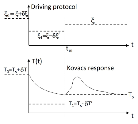
Figure 8: Qualitative plot of the Kovacs protocol. The system starts from a NESS with granular temperature $T_{0}=T_{\text{s}}+\delta T$, corresponding to a driving $\xi_{0}=\xi+\delta\xi$. In the waiting time window, the driving is suddenly decreased to $\xi_{1}=\xi-\delta\xi^{\prime}<\xi$ and the granular temperature approaches the corresponding steady state value $T_{1}=T_{\text{s}}-\delta T^{\prime}<T_{\text{s}}$. At the waiting time, the granular temperature equals its steady value for the driving $\xi$. However, for longer times the granular temperature does not remain flat: it displays a non-monotonic behaviour, the Kovacs hump. The normal case is depicted, in which the temperature displays a maximum, but anomalous behaviour—a minimum instead of a maximum—can also be observed. Note that $\delta T$ and $\delta T^{\prime}$ are defined in such a way that they are both positive.

In the following, we analyse the Kovacs hump in linear response. Note that the theoretical approach presented here essentially differs from that in Refs. [16, 18], where the non-linear case—large jumps in the driving—was investigated. Therein, a perturbative analysis in powers of $a_{2,\text{s}}$ made it possible to derive an analytical expression for the Kovacs hump, but only when the system freely cooled in the waiting time window . The linear response approach developed below, although limited to small jumps in the driving, improves our understanding of the Kovacs effect by connecting the shape of the hump with the properties of the direct relaxation function.

The evolution of the temperature for $\uptau\geq\uptau_{w}$ directly follows from the general linear response scheme in Ref. [38]. Namely, it is given by

$$\delta T(\uptau)=\left(T_{0}-T_{1}\right)\left[\phi_{\theta}(\uptau)-\phi_{\theta}(\uptau_{w})\phi_{\theta}(\uptau-\uptau_{w})\right],$$ (62)

where $\phi_{\theta}$ is the direct relaxation function (i.e., for the one jump experiment), normalised in the sense that $\phi_{\theta}(\uptau=0)=1$. Substitution of Eq. (27) into (62) results, after a little bit of algebra, in

$$\delta\theta(\uptau)=\left(\delta\theta+\delta\theta^{\prime}\right) a_{+}a_{-}\left(e^{\lambda_{+}\uptau_{w}}-e^{\lambda_{-}\uptau_{w}}\right)$$

$$\times\left(e^{\lambda_{+}(\uptau-\uptau_{w})}-e^{\lambda_{-}(\uptau-\uptau_{w})}\right),$$ (63)

where we have employed the dimensionless temperature jumps

$$\delta\theta\equiv\frac{\delta T}{T_{\text{s}}}=\frac{T_{0}-T_{\text{s}}}{T_{\text{s}}},\quad\delta\theta^{\prime}\equiv\frac{\delta T^{\prime}}{T_{\text{s}}}=\frac{T_{\text{s}}-T_{1}}{T_{\text{s}}},$$ (64)

such that $T_{0}-T_{1}=T_{\text{s}}(\delta\theta+\delta\theta^{\prime})$. The time evolution of $\delta\theta(\uptau)$ is non-monotonic: it is the amplitude $a_{-}$ of the second mode of the direct relaxation function $\phi_{\theta}$ that controls the sign of the Kovacs response, since the remainder of the terms on the rhs of Eq. (63) are positive definite. Normal behaviour, i.e. $\delta\theta(\uptau)\geq 0$, is obtained for $a_{-}>0$, i.e. for $\alpha>\alpha_{c}$—see Eq. (29) and Fig. 1. Anomalous behaviour, i.e. $\delta\theta(\uptau)\leq 0$, is obtained for $a_{-}<0$, i.e. for $\alpha<\alpha_{c}$.

The above discussion entails that the anomalous Kovacs response persists in the linear response regime, with its emergence being controlled by the sign of the second mode of $\phi_{\theta}$. Therefore, the anomalous Kovacs response is not a non-linear effect. In fact, the separation between normal and anomalous behaviour is similar to the one found in the non-linear regime [16, 18]: normal behaviour is found for small inelasticity ($\alpha>\alpha_{c}$), whereas anomalous behaviour comes about for large inelasticity ($\alpha<\alpha_{c}$).

The linear response approximation makes it possible to analyse the behaviour of the system for $\uptau\leq\uptau_{w}$. Therein, the system is relaxing towards the NESS corresponding to the lowest temperature $T_{1}=T_{\text{s}}-\delta T^{\prime}$ and the excess kurtosis evolves according to

$$\delta A_{2}(\uptau)=\delta\theta_{1}(0)\frac{a_{+}a_{-}(\lambda_{+}-\lambda_{-})}{M_{12}}\left(e^{\lambda_{+}\uptau_{1}}-e^{\lambda_{-}\uptau_{1}}\right).$$ (65)

This follows from Eq. (35) with the changes brought about by the different steady temperature: the initial temperature jump must be measured with respect to $T_{1}$, i.e. $\delta\theta_{1}(0)=(T_{0}-T_{1})/T_{1}$, and $\tau_{1}$ is the scaled time in Eq. (7) with the substitution $T_{\text{s}}\to T_{1}$. Taking into account Eq. (64) and keeping only linear terms in the deviations,

$$\delta A_{2}(\uptau)=\left(\delta\theta+\delta\theta^{\prime}\right)\frac{a_{+}a_{-}(\lambda_{+}-\lambda_{-})}{M_{12}}\left(e^{\lambda_{+}\uptau}-e^{\lambda_{-}\uptau}\right).$$ (66)

Let us recall that $\delta A_{2}(\uptau)>0$ for all times.

Figure 9: Kovacs hump for large inelasticity. Specifically, the restitution coefficient is $\alpha=0.3$. The circles are simulation results obtained with $N=10^{6}$ particles averaged over $10^{4}$ runs, while the solid line is our theoretical prediction (67). The Kovacs response is anomalous for this large inelasticity, $\alpha<\alpha_{c}$.

Figure 10: Kovacs hump for small inelasticity. Specifically, the restitution coefficient is $\alpha=0.8$. The response is normal in this case, $\alpha>\alpha_{c}$. The circles are simulation results obtained with $N=10^{6}$ particles averaged over $5\times 10^{4}$ runs, whereas the solid line is again Eq. (67).

In what follows, we compare simulation results from the DSMC numerical integration of the Boltzmann-Fokker-Planck equation with our theoretical predictions. Specifically, we plot

$$K_{\theta}(\uptau;\uptau_{w}) \equiv\frac{\delta\theta(\uptau)}{\delta\!A_{2}(\uptau_{w})}$$

$$=\frac{M_{12}}{\lambda_{+}-\lambda_{-}}\left(e^{\lambda_{+}(\uptau-\uptau_{w})}-e^{\lambda_{-}(\uptau-\uptau_{w})}\right),$$ (67)

where we have made use of Eqs. (63) and (66), the latter particularised for $\uptau=\uptau_{w}$. Since $\delta\!A_{2}(\uptau_{w})>0$, we have that $\delta\theta$ and $K_{\theta}$ have the same sign. In order to implement the Kovacs protocol we have set the following values for the noise intensity: $\xi^{2}=0.2$, $(\xi+\delta\xi)^{2}=0.35$, and $(\xi-\delta\xi)^{2}=0.05$. Fluctuations make these larger jumps necessary to numerically observe the time evolution of the excess kurtosis, which is the quantity bringing about the Kovacs effect. As discussed in Sec. III and illustrated in Figs. 5 and 6, linear response still holds in this situation .

The case $\alpha<\alpha_{c}$, i.e. the large inelasticity regime, is shown in Fig. 9. Consistently with our theoretical predictions, the Kovacs response is anomalous, $K_{\theta}<0$, and the agreement between simulations and theory is excellent. The small inelasticity regime, $\alpha>\alpha_{c}$ is illustrated in Fig. 10. Here, the response is normal, $K_{\theta}>0$, and the amplitude of the hump is roughly one order of magnitude smaller than that in Fig. 9.

VII Discussion

We have investigated the relaxation of the granular temperature $T$ and the excess kurtosis $a_{2}$—or, alternatively, of the fourth-moment of the velocity—in the linear response regime. This study has been carried out by employing two different methods. First, in the direct route, we have linearised the evolution equations for small changes of the driving and obtained the analytical solution thereof. Second, in the FDR route, we have derived a generalised FDR, which relates the relaxation functions after a small change in the driving with certain time correlation functions in the NESS.

The theoretical predictions above have been checked against DSMC results. In the simulations, we have considered both the direct and the FDR routes. In the first, we have found a perfect agreement between the simulations and the theoretical predictions. In the second, the agreement is also very good when the normalised relaxation function—equal to unity for the initial time—is compared with the corresponding normalised time correlation in the NESS. However, the initial value of the time correlation does not match that of the relaxation function, because two-body correlations have a non-vanishing contribution. This is analogous to the situation found in the study of the fluctuations of the total energy of the uniformly heated granular gas [67].

The linear relaxation function of the granular temperature in the simulations is almost perfectly fitted by a single exponential, over the whole range of inelasticities. Interestingly, this seems to rule out the possibility of memory effects, since it is well-known that non-exponential relaxation is a prerequisite for the appearance of aging and memory effects—a simple example is the one-dimensional Ising model [20, 23, 24, 50]. Nevertheless, the relaxation function is not exactly exponential: the relaxation has two modes, but the coefficient of the second mode is much smaller than that of the first mode—their ratio varying from $0$ for $\alpha=1$ (the elastic limit) to roughly $0.01$ for $\alpha=0$ (the completely inelastic case). It is this smallness that makes inferring the deviation from the exponential behaviour by looking only at the numerical data problematic. This highlights the difficulty of ruling out the possible emergence of memory effects by investigating only simple, single-jump, relaxation experiments.

Despite its smallness, the non-trivial behaviour of the coefficient of the second mode as a function of the inelasticity and, in particular, its changing sign at the critical value $\alpha_{c}$, as shown in Fig. 1, have important physical consequences. The most striking one is its bringing about the anomalous Kovacs effect in linear response. In molecular systems, there is a clear parallelism between the observed universal properties of the Kovacs hump in experiments—which are done in the non-linear regime—and the general properties that can be rigorously proved in linear response. In particular, its normal character—a well-defined sign that does not change with the system parameters—stem from the equilibrium FDR that ensures that the coefficients of all the modes in the direct relaxation function are positive [47].

Extension of the above parallelism between the “empirical” non-linear results and the theoretical linear response results to athermal systems—like granular fluids or granular matter—suggests that it is precisely the change of sign of the coefficient of the second mode that gives rise in general to the anomalous Kovacs effect, not only for the granular gas that we have considered here. This improves our understanding of the emergence of the anomalous Kovacs effect in athermal systems. Moreover, we have neatly shown that the anomalous behaviour survives in the linear regime, non-linearities are not necessary to bring it about.

A perspective for future work is the resolution of the discrepancy between the initial values of the relaxation function and the corresponding time correlation function that stems from the generalised FDR. To accomplish this goal, it is necessary to go beyond the completely factorised form (47) of the $N$-particle distribution function, including at least two-body correlations—but not only in the NESS, as was done in Ref. [67], but also for a time-dependent situation. Another possible avenue for future development is the analysis of linear response results in other, more complex, intrinsically non-equilibrium systems, like the rough granular gas [68, 69, 70] or active matter [71, 72, 73, 74, 75, 76].

References

- Kubo [1966] R. Kubo, The fluctuation-dissipation theorem, Reports on Progress in Physics 29, 255 (1966).
- Callen [1985] H. Callen, Thermodynamics and an Introduction to Thermostatistics (Wiley, 1985).
- Van Kampen [1992] N. G. Van Kampen, Stochastic processes in Physics and Chemistry (North-Holland, 1992).
- Marconi et al. [2008] U. M. B. Marconi, A. Puglisi, L. Rondoni, and A. Vulpiani, Fluctuation–dissipation: response theory in statistical physics, Physics Reports 461, 111 (2008).
- Goldhirsch and Zanetti [1993] I. Goldhirsch and G. Zanetti, Clustering instability in dissipative gases, Physical Review Letters 70, 1619 (1993).
- Brey et al. [1997] J. J. Brey, J. W. Dufty, and A. Santos, Dissipative dynamics for hard spheres, J. Stat. Phys. 87, 1051 (1997).
- Brilliantov and Pöschel [2004] N. V. Brilliantov and T. Pöschel, Kinetic Theory of Granular Gases (OUP Oxford, 2004).
- Puglisi et al. [2005] A. Puglisi, P. Visco, A. Barrat, E. Trizac, and F. van Wijland, Fluctuations of internal energy flow in a vibrated granular gas, Physical Review Letters 95, 110202 (2005).
- Van Noije and Ernst [1998] T. P. C. Van Noije and M. H. Ernst, Velocity distributions in homogeneous granular fluids: the free and the heated case, Granul. Matter 1, 57 (1998).
- Montanero and Santos [2000] J. M. Montanero and A. Santos, Computer simulation of uniformly heated granular fluids, Granular Matter 2, 53 (2000).
- Goldshtein and Shapiro [1995] A. Goldshtein and M. Shapiro, Mechanics of collisional motion of granular materials. Part 1. General hydrodynamic equations, Journal of Fluid Mechanics 282, 75 (1995).
- García de Soria et al. [2012] M. I. García de Soria, P. Maynar, and E. Trizac, Universal reference state in a driven homogeneous granular gas, Physical Review E 85, 051301 (2012).
- Huthmann et al. [2000] M. Huthmann, J. A. G. Orza, and R. Brito, Dynamics of deviations from the Gaussian state in a freely cooling homogeneous system of smooth inelastic particles, Granular Matter 2, 189 (2000).
- Brilliantov and Pöschel [2000] N. Brilliantov and T. Pöschel, Deviation from Maxwell distribution in granular gases with constant restitution coefficient, Physical Review E 61, 2809 (2000).
- Santos and Montanero [2009] A. Santos and J. M. Montanero, The second and third Sonine coefficients of a freely cooling granular gas revisited, Granular Matter 11, 157 (2009).
- Prados and Trizac [2014] A. Prados and E. Trizac, Kovacs-Like Memory Effect in Driven Granular Gases, Physical Review Letters 112, 198001 (2014).
- Lasanta et al. [2017] A. Lasanta, F. Vega Reyes, A. Prados, and A. Santos, When the Hotter Cools More Quickly: Mpemba Effect in Granular Fluids, Physical Review Letters 119, 148001 (2017).
- Trizac and Prados [2014] E. Trizac and A. Prados, Memory effect in uniformly heated granular gases, Physical Review E 90, 012204 (2014).
- Scherer [1986] G. W. Scherer, Relaxation in glass and composites (Wiley New York, 1986).
- Spohn [1989] H. Spohn, Stretched exponential decay in a kinetic Ising model with dynamical constraint, Communications in Mathematical Physics 125, 3 (1989).
- Kob and Schilling [1990] W. Kob and R. Schilling, Dynamics of a one-dimensional “glass”model: Ergodicity and nonexponential relaxation, Physical Review A 42, 2191 (1990).
- Scherer [1990] G. W. Scherer, Theories of relaxation, J. Non-Cryst. Solids 123, 75 (1990).
- Brey and Prados [1993] J. J. Brey and A. Prados, Stretched exponential decay at intermediate times in the one-dimentional Ising model at low temperatures, Physica A 197, 569 (1993).
- Brey and Prados [1996] J. J. Brey and A. Prados, Low-temperature relaxation in the one-dimensional Ising model, Physical Review E 53, 458 (1996).
- Angell et al. [2000] C. A. Angell, K. L. Ngai, G. B. McKenna, P. F. McMillan, and S. W. Martin, Relaxation in glassforming liquids and amorphous solids, Journal of Applied Physics 88, 3113 (2000).
- Bouchaud [1992] J.-P. Bouchaud, Weak ergodicity breaking and aging in disordered systems, Journal de Physique I 2, 1705 (1992).
- Cugliandolo et al. [1994] L. F. Cugliandolo, J. Kurchan, and F. Ritort, Evidence of aging in spin glass mean-field models, Physical Review B 49, 6331 (1994).
- Prados et al. [1997] A. Prados, J. J. Brey, and B. Sánchez-Rey, Aging in the one-dimensional Ising model with Glauber dynamics, EPL 40, 13 (1997).
- Josserand et al. [2000] C. Josserand, A. V. Tkachenko, D. M. Mueth, and H. M. Jaeger, Memory effects in granular materials, Physical Review Letters 85, 3632 (2000).
- Brey et al. [2007] J. J. Brey, A. Prados, M. I. García de Soria, and P. Maynar, Scaling and aging in the homogeneous cooling state of a granular fluid of hard particles, Journal of Physics A: Mathematical and Theoretical 40, 14331 (2007).
- Ahmad and Puri [2007] S. R. Ahmad and S. Puri, Velocity distributions and aging in a cooling granular gas, Physical Review E 75, 031302 (2007).
- Hecht et al. [2017] R. Hecht, S. F. Cieszymski, E. V. Colla, and M. B. Weissman, Aging dynamics in ferroelectric deuterated potassium dihydrogen phosphate, Physical Review Materials 1, 044403 (2017).
- Lahini et al. [2017] Y. Lahini, O. Gottesman, A. Amir, and S. M. Rubinstein, Nonmonotonic Aging and Memory Retention in Disordered Mechanical Systems, Physical Review Letters 118, 085501 (2017).
- Dillavou and Rubinstein [2018] S. Dillavou and S. M. Rubinstein, Nonmonotonic Aging and Memory in a Frictional Interface, Physical Review Letters 120, 224101 (2018).
- van Bruggen et al. [2019] E. van Bruggen, E. van der Linden, and M. Habibi, Tailoring relaxation dynamics and mechanical memory of crumpled materials by friction and ductility, Soft Matter 15, 1633 (2019).
- Keim et al. [2019] N. C. Keim, J. D. Paulsen, Z. Zeravcic, S. Sastry, and S. R. Nagel, Memory formation in matter, Reviews of Modern Physics 91, 035002 (2019).
- Lulli et al. [2020] M. Lulli, C.-S. Lee, H.-Y. Deng, C.-T. Yip, and C.-H. Lam, Spatial Heterogeneities in Structural Temperature Cause Kovacs’ Expansion Gap Paradox in Aging of Glasses, Physical Review Letters 124, 095501 (2020).
- Plata and Prados [2017] C. A. Plata and A. Prados, Kovacs-Like Memory Effect in Athermal Systems: Linear Response Analysis, Entropy 19, 539 (2017).
- García de Soria et al. [2015] M. I. García de Soria, P. Maynar, S. Mischler, C. Mouhot, T. Rey, and E. Trizac, Towards an H-theorem for granular gases, Journal of Statistical Mechanics: Theory and Experiment , P11009 (2015).
- Kovacs [1963] A. J. Kovacs, Transition vitreuse dans les polymères amorphes. Etude phénoménologique, Fortschritte Der Hochpolymeren-Forschung 3, 394 (1963).
- Kovacs et al. [1979] A. J. Kovacs, J. J. Aklonis, J. M. Hutchinson, and A. R. Ramos, Isobaric volume and enthalpy recovery of glasses. II. A transparent multiparameter theory, Journal of Polymer Science: Polymer Physics Edition 17, 1097 (1979).
- Buhot [2003] A. Buhot, Kovacs effect and fluctuation–dissipation relations in 1d kinetically constrained models, Journal of Physics A: Mathematical and General 36, 12367 (2003).
- Bertin et al. [2003] E. M. Bertin, J. P. Bouchaud, J. M. Drouffe, and C. Godrèche, The Kovacs effect in model glasses, Journal of Physics A: Mathematical and General 36, 10701 (2003).
- Arenzon and Sellitto [2004] J. J. Arenzon and M. Sellitto, Kovacs effect in facilitated spin models of strong and fragile glasses, The European Physical Journal B-Condensed Matter and Complex Systems 42, 543 (2004).
- Mossa and Sciortino [2004] S. Mossa and F. Sciortino, Crossover (or Kovacs) effect in an aging molecular liquid, Physical Review Letters 92, 045504 (2004).
- Aquino et al. [2006] G. Aquino, L. Leuzzi, and T. M. Nieuwenhuizen, Kovacs effect in a model for a fragile glass, Physical Review B 73, 094205 (2006).
- Prados and Brey [2010] A. Prados and J. J. Brey, The Kovacs effect: a master equation analysis, Journal of Statistical Mechanics: Theory and Experiment , P02009 (2010).
- Diezemann and Heuer [2011] G. Diezemann and A. Heuer, Memory effects in the relaxation of the Gaussian trap model, Physical Review E 83, 031505 (2011).
- Di et al. [2011] X. Di, K. Z. Win, G. B. McKenna, T. Narita, F. Lequeux, S. R. Pullela, and Z. Cheng, Signatures of Structural Recovery in Colloidal Glasses, Physical Review Letters 106, 095701 (2011).
- Ruiz-García and Prados [2014] M. Ruiz-García and A. Prados, Kovacs effect in the one-dimensional Ising model: A linear response analysis, Physical Review E 89, 012140 (2014).
- Banik and McKenna [2018] S. Banik and G. B. McKenna, Isochoric structural recovery in molecular glasses and its analog in colloidal glasses, Physical Review E 97, 062601 (2018).
- Song et al. [2020] L. Song, W. Xu, J. Huo, F. Li, L.-M. Wang, M. D. Ediger, and J.-Q. Wang, Activation Entropy as a Key Factor Controlling the Memory Effect in Glasses, Physical Review Letters 125, 135501 (2020).
- Kürsten et al. [2017] R. Kürsten, V. Sushkov, and T. Ihle, Giant Kovacs-Like Memory Effect for Active Particles, Physical Review Letters 119, 188001 (2017).
- Lasanta et al. [2019] A. Lasanta, F. V. Reyes, A. Prados, and A. Santos, On the emergence of large and complex memory effects in nonequilibrium fluids, New Journal of Physics 21, 033042 (2019).
- Garzó [2019] V. Garzó, Granular Gaseous Flows: A Kinetic Theory Approach to Granular Gaseous Flows (Springer International Publishing, Cham, 2019).
- Note [1] This expression for stems from a lengthy kinetic theory calculation [12] or, preferably, from a simple self-consistency argument [16, 18].
- Note [2] They are non-linear in the temperature but linear in the excess kurtosis. This is a consequence of the first Sonine approximation, in which non-linearities in are neglected.
- Note [3] We are employing a notation similar to that introduced in Ref. [38] to investigate the linear response of a general athermal system, at the level of description of the equations for the moments.
- Note [4] The steady value of the granular temperature is an increasing function of the driving, both and have the same sign.
- Kac [2020] M. Kac, Foundations of kinetic theory, in Volume 3 Contributions to Astronomy and Physics, edited by J. Neyman (University of California Press, 2020) pp. 173–200.
- Note [5] The derivation above follow the same lines of the proof of a FDR in non-Hamiltonian systems of Ref. [4]. Therein, the authors consider the response to an initial perturbation of the form .
- Note [6] They do not superimpose as a function of the real time . The definition of the scaled time in Eq. (7\@@italiccorr) involves because the parameter is proportional to . Therefore, the smaller the inelasticity is, the slower the relaxation in real time becomes.
- Note [7] Only the “static”, time-independent, correlations in the NESS of the uniformly heated granular gas have been previously investigated [67].
- Note [8] Aside from the original papers by Kovacs [40, 41], the account of the original experiment can be found in many places, see for example Refs. [19, 22, 47].
- Note [9] For , the system reached the homogeneous cooling state and the specific value in the waiting time window, after a quite short transient.
- Note [10] This can be physically understood in this two-jump experiment, the size of the memory effect is quite small.
- García de Soria et al. [2009] M. I. García de Soria, P. Maynar, and E. Trizac, Energy fluctuations in a randomly driven granular fluid, Molecular Physics 107, 383 (2009).
- Kremer et al. [2014] G. M. Kremer, A. Santos, and V. Garzó, Transport coefficients of a granular gas of inelastic rough hard spheres, Physical Review E 90, 022205 (2014).
- Reyes et al. [2014] F. V. Reyes, A. Santos, and G. M. Kremer, Role of roughness on the hydrodynamic homogeneous base state of inelastic spheres, Physical Review E 89, 020202 (2014).
- Torrente et al. [2019] A. Torrente, M. A. López-Castaño, A. Lasanta, F. V. Reyes, A. Prados, and A. Santos, Large Mpemba-like effect in a gas of inelastic rough hard spheres, Physical Review E 99, 060901 (2019).
- Baskaran and Marchetti [2008] A. Baskaran and M. C. Marchetti, Enhanced Diffusion and Ordering of Self-Propelled Rods, Physical Review Letters 101, 268101 (2008).
- Baskaran and Cristina Marchetti [2010] A. Baskaran and M. Cristina Marchetti, Nonequilibrium statistical mechanics of self-propelled hard rods, Journal of Statistical Mechanics: Theory and Experiment , P04019 (2010).
- Ihle [2011] T. Ihle, Kinetic theory of flocking: Derivation of hydrodynamic equations, Physical Review E 83, 030901 (2011).
- Marchetti et al. [2013] M. C. Marchetti, J. F. Joanny, S. Ramaswamy, T. B. Liverpool, J. Prost, M. Rao, and R. A. Simha, Hydrodynamics of soft active matter, Reviews of Modern Physics 85, 1143 (2013).
- Ihle [2016] T. Ihle, Chapman–Enskog expansion for the Vicsek model of self-propelled particles, Journal of Statistical Mechanics: Theory and Experiment , 083205 (2016).
- Bonilla and Trenado [2019] L. L. Bonilla and C. Trenado, Contrarian compulsions produce exotic time-dependent flocking of active particles, Physical Review E 99, 012612 (2019).