Identification of The Number of Wireless Channel Taps Using Deep Neural Networks

Abstract

In wireless communication systems, identifying the number of channel taps offers an enhanced estimation of the channel impulse response (CIR). In this work, efficient identification of the number of wireless channel taps has been achieved via deep neural networks (DNNs), where we modified an existing DNN and analyzed its convergence performance using only the transmitted and received signals of a wireless system. The displayed results demonstrate that the adopted DNN accomplishes superior performance in identifying the number of channel taps, as compared to an existing algorithm called Spectrum Weighted Identification of Signal Sources (SWISS).

I Introduction

The identification of the number of channel taps is a challenging task in real-time with fast channel variations. Precise channel estimation with a better restoration of transmitted signals is possible by identifying the number of taps for unknown environments with no prior information. Therefore, an effective technique to recognize these taps is needed. Various wireless channel identification techniques, like [1, 2, 3], assume prior information at the receiver about the multipath delay profile for the channel. However, this profile is usually unknown in practical use cases.

Motivated by the potential improvements that can be accomplished over the state-of-the-art, this paper proposes a deep neural network (DNN) to identify a sparse channel parameter called the number of taps from transmitted and received data of a wireless system. Our proposed identification technique enhances the spectral efficiency of the communication system since the adopted DNN requires no extra transmitted signals other than the channel input and output data.

Deep learning (DL) can generate extremely high-level data representations from a massive amount of data. More specifically, the DNNs can create maximally sparse representations of the signals of interest. To reflect our approach of DNN modeling, we used the basic network in [4] for finding the maximum sparsity. The DNN in [4] unfolds the high-complexity Iterative Hard Thresholding (IHT) algorithm given in [5]. The research study [4] shows the superior theoretical and empirical performance of this DNN compared to the IHT method. Also, the DNN promotes the maximal sparsity of its input with incomparable complexity.

To highlight the advantages of the adopted DNN in the proposed identification solution, we chose to compare its performance with an existing algorithm called Spectrum Weighted Identification of Signal Sources (SWISS) [6, 7]. The SWISS algorithm solves the identification problem of path-number by determining the optimum combination of the discrete Fourier transform (DFT) components in the weighted DFT of the received signal. The resultant signal represents the reconstructed channel signal, which has the minimum Euclidean distance to the received signal. The number of channel paths is then identified by calculating the number of significant components in the weight vector. Similar to the proposed DNN-based method, the SWISS algorithm does not need prior information about the number of channel taps.

Unlike the existing SWISS algorithm, our main contributions to the literature are summarized as follows:

• A new DNN-based technique is proposed to solve the multi-label classification problem of identifying the number of wireless channel taps. In the proposed technique, prior information is assumed to be not available.

• A measurement-based simulator has been used for channel data generation, which is used for training, validating, and testing the adopted DNN.

• The proposed DNN-based technique has significantly improved accuracy performance over the SWISS algorithm [6] while maintaining moderate complexity.

The rest of this paper is organized as follows. Section II provides a summary of the fundamental system model. Section III presents the datasets generation and simulation setup. The simulation results are presented in Section IV. Finally, Section V provides a conclusion with some future directions.

II System Model

The deterministic parameters of wireless channels include the number of taps, taps delays, and delay spread. Different taps of the channel impulse response (CIR) experience pathloss and time-variations in a multipath radio environment. The CIR could be formulated as [8]

$$h(\tau,t)=\sum_{l=0}^{L-1}\beta_{l}\thinspace\mu_{l}(t)\thinspace\delta\left(\tau-\tau_{l}\right),$$ (1)

where $L$ represents the total number of channel taps, $\beta_{l}$ and $\tau_{l}$ represent pathloss and delay of $l$-th channel tap, respectively. $\mu_{l}(t)$ represents the time variation of the $l$-th channel tap, and $\delta(.)$ is the delta function.

Generally, double-directional CIR is adopted as a fundamental deterministic description of the channel in modern wireless communication systems. This CIR can be formulated as [9]

$$h(\tau,t,\psi,\theta)=\sum_{l=0}^{L-1}\beta_{l}\mu_{l}(t)\delta\left(\tau-\tau_{l}\right)\delta\left(\theta-\theta_{l}\right)\delta\left(\psi-\psi_{l}\right),$$ (2)

where $\theta$ and $\psi$ represent the angle of departure and angle of arrival, respectively.

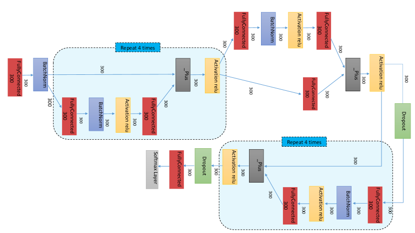
Figure 1: Basic network structure [4].

The received signal faded by a multipath channel, assuming a noise-free system for simplification, can be represented by

$$y(t)=x(t)\ast h(\tau,t,\psi,\theta),$$ (3)

where $\ast$ represents the convolution operator and $x(t)$ is the transmitted signal.

With different wireless environments, the parameter $L$ varies due to different propagation paths. Therefore, it is necessary to identify $L$ in the CIR since it is usually unknown in practical scenarios.

The input samples to the DNN are represented as

$$\mathcal{D}_{j}=\left\{\mathbf{x}^{(j)},\mathbf{y}^{(j)}\right\}_{j}.$$ (4)

where $\mathbf{x}^{(j)}$ and $\mathbf{y}^{(j)}$ represent the vector form of $x(t)$ and $y(t)$ for the $j$-th class of channels, respectively. These DNN inputs are mapped to the desired output that is characterized by a specific number of taps.

Our problem is focused on finding a maximally sparse vector $\mathbf{c}^{*}\in\mathbb{R}^{m}$ such that the observed vector $\mathbf{r}\in\mathbb{R}^{n}$ can be represented by the fewest number of features in a feasible region. In general, the aforementioned problem is considered an optimization problem given by [4] as

$$\begin{array}[]{cl}\underset{\mathbf{c}}{\operatorname{min}}&\|\mathbf{c}\|_{0}\\ \text{s.t.}&\mathbf{r}=\mathbf{W}\mathbf{c}\end{array}$$ (5)

where $||\mathbf{c}||_{0}$ denotes $l^{0}$ norm, which counts the non-zero elements in $\mathbf{c}$, reflects the number of channel taps. $\mathbf{W}\in\mathbb{R}^{n\times m}$ is a known, overcomplete dictionary of feature vectors. These vectors provide an indirect measurement for CIR.

The equivalent problem of (5) can be written as [4]

$$\begin{array}[]{ll}\underset{c}{\operatorname{min}}&\frac{1}{2}\|\mathbf{r}-\mathbf{W}\mathbf{c}\|_{2}^{2}\\ \text{s.t.}&\|\mathbf{c}\|_{0}\leqslant s\end{array}$$ (6)

where $s$ represents a pre-determined integer to control the sparsity of $\mathbf{c}$.

If there is a strong coherence between columns of $\mathbf{W}$, then the sparse recovery estimation shown in (6) could be significantly poor. One possible solution to the observed high correlations in the dictionary is to exploit data for training a transformation of a dictionary, which can enhance its restricted isometry property constant. It has been proven that the existing DNNs provide such a solution [4].

Inspired by the featured characteristics offered by the DNN in [4], we employ a similar DNN, and its detailed structure can be found in Fig. 1. To improve the performance of the used network, we incorporate some modifications by introducing two Dropout layers to the DNN proposed in [4]. These Dropout layers offer regularization to avoid overfitting.

The adopted DNN includes fully-connected layers interleaved with non-linear transformation layers. In particular, the feed-forward design comprises fully-connected layers with 300 neurons and batch normalization. The batch normalization is incorporated in the designed DNN to provide a reasonable initialization. Simple Rectilinear units (ReLU) tend to promote sparse features by deactivating weights with negative values. The used non-linear unit can be represented as

$$f(u)=u\operatorname{sign}(\max\{|u|-\alpha,0\}),$$ (7)

where sign(.) represents the sign function and $\alpha$ denotes the shrinkage parameter.

Also, a final softmax layer is included, which yields a vector $\mathbf{p}$, where $p_{j}\in[0,1]$ provides an assessment of the likelihood that the subject channel belongs to the $j$-th class of channels. For the loss function, we used the cross-entropy loss function, which is defined as

$$CE=-\sum_{j=1}^{C}g_{j}\log\left(p_{j}\right),$$ (8)

where $C$ and $g_{j}$ represent the number of classes and ground truth for the $j$-th class, respectively, for a given observation.

III Methodology

In this section, the datasets generation and simulation setup are presented.

III-A Training Data Generation

Here, we import the measurement-based channel datasets from the NYUSIM simulator [10]. This simulator is an open-source 5G and 6G channel model software. The existing channel simulators such as Quasi Deterministic Radio channel Generator (QuaDRiGa) [11], Simulation of Indoor Radio Channel Impulse Response Models (SIRCIM) [12], etc. have not been developed based on extensive propagation measurements at centimeter-wave to millimeter-wave (mmWave) bands in diverse scenarios for 5G wireless systems. However, NYUSIM has been built based on extensive field measurements at mmWave bands in different outdoor environments, including urban microcell, urban macrocell, and rural macrocell environments.

Another feature found in NYUSIM is that it can recreate wideband power delay profiles/CIRs and channel statistics for a broad set of frequencies, beamwidths, bandwidths, wireless channel scenarios, etc. [10]. Moreover, the NYUSIM simulator generates a realistic three-dimensional statistical spatial CIRs as represented in (2). These generated CIRs include the clustering approach and physically-based pathloss model, which can be applied for the frequency range 0.5-100 GHz.

III-B Simulation setup

The parameters of the conducted simulations are chosen to be similar to that of the default simulation setup in [10] for the spatial channel model using NYUSIM. The selected parameters are suitable in the 3rd Generation Partnership Project (3GPP) and other standard bodies as well as industrial/academic simulations. The transmitted signals with a specific size of $1000\times 1$ are sent through different wideband frequency-selective channels with the generated CIR of a length corresponding to the number of multipath components. Then, the complex-valued received signals with their corresponding number of channel taps are used as the training dataset. The inputs of the DNN are set as transmitted and received signals’ samples. On the other hand, the output corresponds to the number of wireless channel taps. The received signal size is 1499, where real values are concatenated with its imaginary values. The dataset includes several channel realizations, limited to 222 different channel classes in terms of the number of channel taps. The DNN is implemented and trained using the Keras framework on Google Colaboratory service graphical processing unit (GPU).

The specifications of the adopted DNN are defined as follows: The chosen number of neurons is sufficiently large for an adequate generalization performance. However, this number should not be very large not to increase the computational complexity or cause overfitting. The training process is performed until a stop criterion is satisfied.

The hyper-parameters selection is critical to the performance of DNN and they are determined empirically. The batch size is $128$ and the learning rate follows a scheduler. The initial value of learning rate is $0.001$ and decreases by a factor of 0.8 when the training accuracy forms a plateau for 18 epochs. Our DNN is trained with Adam optimizer [13] due to its computational efficiency, fast, and smooth convergence. The generated dataset size is $30$K observations which are divided into $70\%$ training data, $15\%$ validation data, and $15\%$ test data.

The developed DNN is also compared with the existing SWISS algorithm [6]. Table I shows the simulation parameters of the SWISS algorithm. It is proven in [7] that choosing a proper threshold ($\eta$) becomes a more difficult problem as the number of paths increases, which limits the achievable accuracy performance of the SWISS algorithm.

TABLE I: The considered parameters for the SWISS algorithm

Threshold ($\eta$)	0.995
Number of pilots	128
Pilot energy	1
Modulation type	BPSK
Number of OFDM subcarriers	512
Number of OFDM symbols	2
Root-finding method	Newton’s method [14]
Initial guess in Newton’s method	1
Number of iterations in Newton’s method	10
Error tolerance in Newton’s method	0.001

IV Simulation Results

For multi-label classification problem, the accuracy is taken as one of the key performance metrics in the literature [4]. Fig. 2 shows the convergence performance after $1500$ training epochs. The training accuracy is around $70\%$, about 8 points higher than the validation accuracy. When the number of epochs increases, both training and validation losses notably decrease. The achieved test accuracy is almost $62\%$. These preliminary results prove that our DNN converges to provide significantly higher accuracy than the existing SWISS algorithm under practical conditions where the signals are impaired by the frequency-selective fading channels. More specifically, the SWISS algorithm is a less efficient technique since pilot symbols are needed for accurate path-number identification. The accuracy obtained from NYUSIM datasets using the SWISS algorithm is low (40.54%), which is much less than the value obtained by the proposed DNN-based approach.

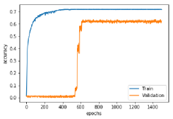
(a) Change in training/validation accuracy during training.

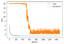
(b) Change in training/validation loss during training.

Figure 2: The convergence performance of the adopted DNN.

However, the accuracy metric can not represent the tolerance in results. The predicted number of taps that falls within a tolerance margin from the ground truth can be seen using a confusion matrix. The obtained confusion matrix for the test set is shown in Fig. 3. However, the bias effect at the bottom left in Fig. 3 can be explained by the nature of the channels generated from NYUSIM. These channels can have an unbalanced share of generation, causing the repetition of the number of taps in an unfair way. Thus, the bias leads to a misprediction that ultimately lowers the accuracy. Despite this unwanted effect, the overall performance of the network tends to provide a solution for the identification of the number of channel taps.

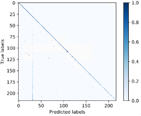
Figure 3: Normalized confusion matrix for test set in the proposed DNN-based method.

Furthermore, the computational complexity of the existing SWISS algorithm is very high. Particularly, the SWISS technique requires implementing one of the root-finding methods such as the Newton method to get the optimal dual variable for each class, thereby increasing the computational overhead. Also, these root-finding methods need to have initial guesses, error tolerance, and several iterations to converge to the optimal dual variable. Furthermore, the SWISS algorithm requires several iterations to reach the desired accuracy for each class. On the other hand, the designed DNN saves computational complexity because it executes a constant number of matrix multiplications, independent of the channel’s class.

V Conclusion

In this paper, an end-to-end communication system is trained through a newly developed DNN to identify the number of channel taps. We achieved an improved accuracy and loss performance over the existing SWISS algorithm in identifying the number of channel taps. Our DNN system is fed by a measurement-based training dataset. The proposed method can be applied for different channel types without the need for a prior analysis. Also, the identified number of taps could help track the time variations of the wireless channel caused by the Doppler effect. The developed DNN has the potential to identify not only the number of multipath components but also their corresponding locations. As another future direction, the impacts of the noise on the proposed solution can be analyzed.

References

- [1] Z. Xiao, H. Wen, A. Markham, N. Trigoni, P. Blunsom, and J. Frolik, “Non-line-of-sight identification and mitigation using received signal strength,” IEEE Trans. Wireless Commun., vol. 14, no. 3, pp. 1689–1702, 2015.
- [2] A. Li, C. Dong, S. Tang, F. Wu, C. Tian, B. Tao, and H. Wang, “Demodulation-free protocol identification in heterogeneous wireless networks,” Comput. Commun., vol. 55, pp. 102–111, 2015.
- [3] D. Li, G. Wu, J. Zhao, W.-H. Niu, and Q. Liu, “Wireless channel identification algorithm based on feature extraction and BP neural network.” JIPS, vol. 13, no. 1, pp. 141–151, 2017.
- [4] B. Xin, Y. Wang, W. Gao, D. Wipf, and B. Wang, “Maximal sparsity with deep networks?” in Proc. Adv. Neural Inf. Process. Syst. (NIPS), Barcelona, Spain, 2016, pp. 4340–4348 (full version at arXiv:1605.01 636).
- [5] T. Blumensath and M. E. Davies, “Iterative hard thresholding for compressed sensing,” Appl. Comput. Harmon. Anal., vol. 27, no. 3, pp. 265–274, 2009.
- [6] Z. Cheng, J. Huang, M. Tao, and P. Kam, “SWISS: Spectrum weighted identification of signal sources for mmWave systems,” in 2018 IEEE Wireless Commun. Netw. Conf. (WCNC), 2018, pp. 1–6.
- [7] Z. Cheng, M. Tao, and P. Kam, “Channel path identification in mmWave systems with large-scale antenna arrays,” IEEE Trans. Commun., pp. 1–1, 2020.
- [8] N. M. Idrees, M. R. Petit, and A. Springer, “Identification of taps in time-variant multipath channels for 3GPP LTE-downlink,” in Proc. Eur. Wireless 2015; 21th Eur. Wireless Conf., Budapest, Hungary, 2015, pp. 1–6.
- [9] A. Adhikary, E. Al Safadi, M. K. Samimi, R. Wang, G. Caire, T. S. Rappaport, and A. F. Molisch, “Joint spatial division and multiplexing for mm-Wave channels,” IEEE J. Sel. Areas Commun., vol. 32, no. 6, pp. 1239–1255, 2014.
- [10] “Open source downloadable 5G channel simulator software,” https://wireless.engineering.nyu.edu/nyusim-5g-and-6g/, accessed: 2020-05-11.
- [11] S. Jaeckel, L. Raschkowski, K. Börner, and L. Thiele, “QuaDRiGa: A 3-D multi-cell channel model with time evolution for enabling virtual field trials,” IEEE Trans. Antennas Propag., vol. 62, no. 6, pp. 3242–3256, 2014.
- [12] T. S. Rappaport, S. Y. Seidel, and K. Takamizawa, “Statistical channel impulse response models for factory and open plan building radio communicate system design,” IEEE Trans. Commun., vol. 39, no. 5, pp. 794–807, 1991.
- [13] D. P. Kingma and J. Ba, “Adam: A method for stochastic optimization,” in Proc. Int. Conf. Learn. Represent. (ICLR), San Diego, CA, USA, 2015, pp. 1–15 (full version at arXiv:1412.6980).
- [14] N. Kollerstrom, “Thomas simpson and ‘newton’s method of approximation’: an enduring myth,” The Br. J. Hist. Sci., vol. 25, no. 3, p. 347–354, 1992.