Density Distribution in Soft Matter Crystals and Quasicrystals

Abstract

The density distribution in solids is often represented as a sum of Gaussian peaks (or similar functions) centred on lattice sites or via a Fourier sum. Here, we argue that representing instead the logarithm of the density distribution via a Fourier sum is better. We show that truncating such a representation after only a few terms can be highly accurate for soft matter crystals. For quasicrystals, this sum does not truncate so easily, nonetheless, representing the density profile in this way is still of great use, enabling us to calculate the phase diagram for a 3-dimensional quasicrystal forming system using an accurate non-local density functional theory.

The form of the average (probability) density distribution $\rho({\bf r})$ of particles in crystalline and quasicrystalline solids depends crucially on various factors such as temperature, pressure and the nature of the particle interactions. Many important material properties are in turn sensitively related to the form of $\rho({\bf r})$. For example, the Lindemann criterion Hansen and McDonald (2013); Singh (1991); Löwen (1994) identifies the melting of a crystal in terms of the widths of the peaks in $\rho({\bf r})$, which depend sensitively on the distance in the phase diagram between the current state and where solid–liquid phase coexistence occurs.

It has been known for some time that in a uniform solid, $\rho({\bf r})$ can be represented well by sums of Gaussian peaks centred on the lattice sites Hansen and McDonald (2013); Singh (1991); Löwen (1994); Tarazona (2000), i.e.,

$$\rho({\bf r})=\sum_{l}n\left(\frac{\alpha}{\pi}\right)^{3/2}e^{-\alpha({\bf r}-{\bf R}_{l})^{2}},$$ (1)

where $\alpha$ controls the peak widths and $\{{\bf R}_{1},{\bf R}_{2},\dots\}=\{{\bf R}_{l}\}$ is the set of vectors of the lattice sites in the solid. For a crystal these are the set of lattice vectors and $n$ is the average number of particles per lattice site. If the particles have a hard core then $n\leq 1$, but for the soft penetrable particles which model polymeric molecules in solution Likos (2001); Mladek et al. (2006); Lenz et al. (2012) considered here, $n>1$. The Gaussian form (1) and its anisotropic generalisations  Singh (1991); Löwen (1994); Tarazona (2000) are fairly accurate deep in a crystal phase, but are less accurate close to melting.

The other standard representation, due to its periodicity, is to express $\rho({\bf r})$ as a Fourier sum Hansen and McDonald (2013); Singh (1991):

$$\rho({\bf r})=\sum_{j}{\hat{\rho}}_{j}\exp(i{\bf k}_{j}\cdot{\bf r}),$$ (2)

where $\{{\bf k}_{j}\}$ is the set of reciprocal lattice vectors (RLVs) for the crystal, including ${\bf k}=0$, and ${\hat{\rho}}_{j}$ are the Fourier coefficients. For example, in a simple cubic crystal, these wavevectors form a cubic lattice, and the smallest non-zero wavenumber is related to the size of the unit cell.

Both the representations above become more involved when considering quasicrystals (QCs). These have the spatial order of crystals but they lack periodicity, so in QCs the set of vectors $\{{\bf R}_{l}\}$ is aperiodic and Eq. (1) needs to be modified to allow the heights and widths of the peaks to vary in space, replacing $(n,\alpha)$ by $(\{n_{l}\},\{\alpha_{l}\})$. The representation in Eq. (2) can still be used for QCs, with the RLVs indexed by up to six integers Steurer and Deloudi (2009); Jiang and Zhang (2018).

The density peaks of a solid can be rather sharp, so the Fourier sum representation  (2) requires a large number of terms to be accurate. Here, we advocate the following alternative ansatz as being more useful and accurate than either (1) or (2) for crystal and QC density distributions:

$$\rho({\bf r})=\rho_{0}\exp\bigg{[}\sum_{j}{\hat{\phi}}_{j}\exp(i{\bf k}_{j}\cdot{\bf r})\bigg{]},$$ (3)

namely, we represent the logarithm of the density as a Fourier sum over the RLVs, with Fourier coefficients ${\hat{\phi}}_{j}$ and $\rho_{0}$ an arbitrary reference density.

The advantage of representation (3) is that it excels both deep in the crystalline region of the phase diagram, where (1) is accurate, and also close to melting, where the peaks broaden and (2) becomes viable. We show below that for the soft matter systems considered here, retaining only a few terms in the sum in (3) can be remarkably accurate in both regimes. In Archer et al. (2019) we showed that simply retaining wavenumber zero and one other wavenumber in (3) quantitatively agrees with a fully resolved representation of the density in lamellar phases, both near and far from melting. We show here that minimal extra effort is required for crystals such as face-centered cubic (FCC) and body-centered cubic (BCC), although it transpires that more effort is needed for dodecagonal QCs and icosahedral quasicrystals (IQCs).

In what follows, we explain the procedure to determine $\rho({\bf r})$ in the framework of density functional theory (DFT) Evans (1979, 1992); Hansen and McDonald (2013). We show that a severely truncated and simplified ansatz based on (3) allows for an accurate and efficient determination of the 3-dimensional (3D) density distributions, and compares well with existing results Mladek et al. (2006); Pini et al. (2015). Additionally, we show how this strongly nonlinear theory (SNLT) enables efficient computation of the phase diagram in a system that is capable of forming both 3D crystals and IQCs.

The central quantity in DFT is the Helmholtz free energy, expressed as a functional of the density:

$${\cal F}[\rho]=k_{B}T\int\rho\left(\ln(\Lambda^{3}\rho)-1\right)\text{d}{\bf r}+{\cal F}_{\text{ex}}[\rho]+\int\rho U\text{d}{\bf r}.$$ (4)

The first term is the ideal-gas contribution, with $\Lambda$ the thermal de Broglie wavelength, $k_{B}$ Boltzmann’s constant and temperature $T$. ${\cal F}_{\text{ex}}$ is the excess contribution due to particle interactions and the third term is from any external potential $U({\bf r})$. We set $U=0$, as we are interested only in bulk behaviour. The equilibrium density profiles minimize the grand potential $\Omega[\rho]={\cal F}[\rho]-\mu\int\rho\text{d}{\bf r}$, where $\mu$ is the chemical potential, and thus satisfy the Euler–Lagrange equation

$$\ln(\Lambda^{3}\rho)-c^{(1)}[\rho]-\beta\mu=0,$$ (5)

where $\beta=(k_{B}T)^{-1}$ and $c^{(1)}[\rho]\equiv-\beta\delta{\cal F}_{\text{ex}}/\delta\rho$ is the one-body direct correlation function Evans (1979, 1992); Hansen and McDonald (2013). Taking a functional derivative of (5) w.r.t. $\rho$ and then integrating again yields a formally exact expression for $c^{(1)}[\rho]$ that can be rearranged to give

$$\rho({\bf r})=\rho_{0}\exp\bigg{[}\int\text{d}{\bf r}^{\prime}(\rho({\bf r}^{\prime})-\rho_{0})\int_{0}^{1}\textrm{d}\lambda c^{(2)}({\bf r},{\bf r}^{\prime};\rho_{\lambda})\bigg{]},$$ (6)

which is obtained by thermodynamic integration (details in the supplementary information Subramanian et al. (2021)) along a sequence of states with profiles $\rho_{\lambda}\!\!\!=\!\!(1-\lambda)\rho_{0}\!+\!\lambda\rho$. Here, $c^{(2)}({\bf r},{\bf r}^{\prime};\rho_{\lambda})$ is the pair direct correlation function for the inhomogeneous systems along this path Hansen and McDonald (2013); Singh (1991). For a system with interparticle pair-potential $v(r)$, the function $c^{(2)}({\bf r},{\bf r}^{\prime};\rho_{\lambda})\sim-\beta v(|{\bf r}-{\bf r}^{\prime}|)$ for large $|{\bf r}-{\bf r}^{\prime}|$ and is finite for all $({\bf r},{\bf r}^{\prime})$. Thus, the spatial integral inside the exponential in Eq. (6) has the effect of smearing the sharp peaks in $(\rho({\bf r})-\rho_{0})$ and so is more slowly varying than the density, meaning it can be represented accurately via a Fourier sum with fewer terms. The exponential of this smooth function is then the sharply peaked density.

The first term in (5) provides further motivation for the ansatz (3). Substituting $\rho=\rho_{0}\exp(\phi)$ into (5) (without assuming the system is periodic), we obtain

$$\ln(\Lambda^{3}\rho_{0})+\phi-c^{(1)}[\rho_{0}e^{\phi}]-\beta\mu=0.$$ (7)

Fourier transforming gives

$${\hat{\phi}}-\widehat{c^{(1)}[\rho_{0}e^{\phi}]}-\beta\mu^{*}\delta({\bf k})=0,$$ (8)

where the circumflex denotes the Fourier transform. We define $\beta\mu^{*}=\beta\mu-\ln(\Lambda^{3}\rho_{0})$, i.e. the chemical potential with a constant subtracted, and $\delta({\bf k})$ is a Dirac delta function. When the system is periodic, we can replace the Fourier transforms in (8) by Fourier sums and the Dirac delta becomes the Kronecker delta $\delta_{{\bf k},0}$. With the ansatz (3), the unknown Fourier amplitudes $\hat{\phi}_{j}$, are found by solving Eq. (8). The advantage of this is that we are working with, rather than against, the physics, and fewer modes in (3) are needed to resolve $\rho({\bf r})$ accurately.

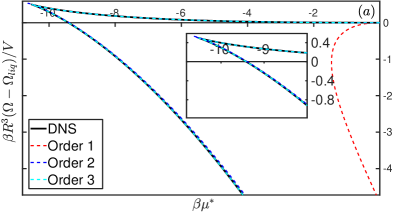
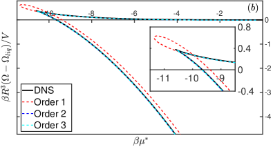
Figure 1: Specific grand potential $\beta R^{3}(\Omega-\Omega_{liq})/V$ (where $V$ is the volume) for $\beta\epsilon=1$ as a function of the chemical potential $\beta\mu^{*}$ for ($a$) FCC crystals and ($b$) BCC crystals in the GEM-4 model, at order 1, 2 and 3 in SNLT, compared with fully resolved direct numerical solutions (DNS) of (10). All our results for crystal properties from order 3 SNLT are indistinguishable from the DNS.

Here, our strongly nonlinear theory (SNLT) is a severe (but controlled) truncation of (3), along with the requirement that Fourier modes whose indices are permutations of each other have equal amplitude. We refer to the level of truncation as the ‘order’ of the SNLT. In the supplementary material Subramanian et al. (2021) we give a detailed exposition of SNLT and Matlab code applying it to the FCC crystal.

To illustrate the advantage of SNLT, we consider two different model systems in 3D: (i) the generalized exponential model with exponent 4 (GEM-4) Mladek et al. (2006); Pini et al. (2015), which enables to compare our SNLT results with those of Ref. Pini et al. (2015), where an unconstrained minimization of $\Omega$ was performed, and (ii) a modified Barkan–Engel–Lifshitz (BEL) Barkan et al. (2014) model designed to promote the formation of IQCs. For both we use the random phase approximation for the excess free energy

$${\cal F}_{\text{ex}}[\rho]=\frac{1}{2}\int\int\rho({\bf r})v(|{\bf r}-{\bf r}^{\prime}|)\rho({\bf r}^{\prime})\text{d}{\bf r}^{\prime}\text{d}{\bf r}\,,$$ (9)

which is accurate for soft-core systems Likos (2001). For particles with a hard-core, one should instead use an alternative approximation for ${\cal F}_{\text{ex}}[\rho]$, e.g. one based on the highly accurate fundamental measure functionals for hard-spheres Evans (1992); Hansen and McDonald (2013); Roth (2010); see also Denton and Hafner (1997a, b); Denton and Löwen (1998); Roth and Denton (2000) for hard-core systems that form QCs. Taking (7) with (9) yields

$$\phi({\bf r})+\rho_{0}\beta\!\!\int\!v(|{\bf r}-{\bf r}^{\prime}|)e^{\phi({\bf r}^{\prime})}\text{d}{\bf r}^{\prime}-\beta\mu^{*}=0,$$ (10)

recalling that $\exp(\phi)$ is proportional to the density.

The GEM-4 is a simple model of dendrimers in solution, treating the effective interactions between the centers of mass via the pair potential $v(r)=\epsilon\exp(-r^{4}/R^{4})$, with $\epsilon$ denoting the strength of the interaction and $R$ its range. Figure 1 shows the GEM-4 grand potential minus that of the uniform liquid state per unit volume ($V$), $\beta R^{3}(\Omega-\Omega_{liq})/V$, versus the chemical potential $\beta\mu^{*}$ for successive orders of SNLT calculations for FCC and BCC crystals, compared with full numerical solutions of Eq. (10) (an unconstrained minimization, using the approach described in Archer et al. (2019)). We see that the order 1 SNLT approximation (red dashes) fails to describe the crystal accurately, especially for the FCC, but the order 2 and 3 SNLT perform significantly better, to the extent that order 3 calculations (cyan dashes) overlap with the full numerical solutions (black solid line). Using this accurate order 3 SNLT, for $\beta\epsilon=1$ we find that the uniform liquid state transitions to a BCC phase at $\beta\mu^{*}=-9.67$, which itself then transitions to a FCC phase at $\beta\mu^{*}=-5.06$. The corresponding coexisting densities at the liquid–BCC transition are, $R^{3}{\bar{\rho}}_{\text{liq}}=5.55$ and $R^{3}{\bar{\rho}}_{\text{BCC}}=6.10$, while for the BCC–FCC transition we have, $R^{3}{\bar{\rho}}_{\text{BCC}}=7.65$, $R^{3}{\bar{\rho}}_{\text{FCC}}=7.70$. These SNLT values agree well with results from Pini et al. Pini et al. (2015) and can easily be rescaled to obtain corresponding values at other temperatures Archer et al. (2019). Other periodic structures, such as lamellar, columnar hexagons and simple cubic crystals, are never global minima of the grand potential.

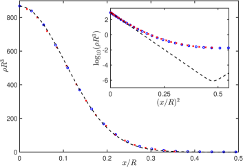
Figure 2: The density profile $\rho$ in a FCC crystal as a function of $x/R$, where $x$ is the distance along a path joining two nearest neighboring density peaks and $R$ is the range parameter in the pair potential, for $\beta\epsilon=1$ and $R^{3}\bar{\rho}=8.3$. The red crosses are the unconstrained minimization results from Figs. 2 and 3 in Pini et al. (2015), the blue circles are the order 3 SNLT results and the black dashed line is the Gaussian form (1). The inset shows $\log_{10}(\rho R^{3})$ as a function of $(x/R)^{2}$, where (1) is a straight line.

Figure 2 shows the density distribution $\rho$ as a function of the interpeak distance $x$ in the FCC crystal, calculated from SNLT (blue circles), from the unconstrained minimisation in Figs. 2 and 3 of Ref. Pini et al. (2015) (red crosses), and from assuming the Gaussian form (1) (dashed black line). Both SNLT and the Gaussian form (1) match Pini et al. (2015) well on the scale of the main plot. However, in the inset we plot $\log_{10}\rho$ as a function of $x^{2}$, which highlights the density between peaks, where we observe that the results of Pini et al. (2015) and SNLT both deviate significantly from the Gaussian form. This highlights an important weakness of representation (1): it underestimates the density between peaks by several orders of magnitude. The density between peaks gives the particle hopping rate between peaks, thus errors in calculating this leads to errors in the diffusion coefficient and related transport properties.

Figure 3 shows the maximum and minimum of $\rho$ as a function of $\beta\mu^{*}$ obtained by three different methods, to compare the regimes under which the different representations of $\rho$ are valid. The inset compares their grand potentials. The Gaussian representation (1) (blue solid lines) recovers the maximum of the density profile correctly, but underestimates the minimum significantly, in line with Fig. 2. This form also leads to an overestimate in the value of the grand potential, particularly near to melting. The red dashed lines are results from the crystal approximation method of Ref. Jiang and Si (2020) employing the representation (2), also truncated at order 3. This gives the unstable lower solution branch well, but not the upper solution branch (going to much higher order is required to obtain the stable upper branch accurately Archer et al. (2019)). In contrast, the black solid line order 3 SNLT accurately captures the form of the density distribution for both branches, near and far away from melting.

Even though the density $\rho$ varies over many orders of magnitude, fewer than a dozen independent Fourier amplitudes in (3) are needed to represent it, while a full Fourier representation (2) requires $\mathcal{O}(48^{3})$ modes to resolve the peaks accurately. On the other hand, using sums of Gaussians (1) requires even fewer degrees of freedom (only $\alpha$, $n$ and $|{\bf R}_{l}|$), but as Fig. 3 shows, this representation is less accurate close to melting, particularly in determining the minimum of $\rho$ and the grand potential.

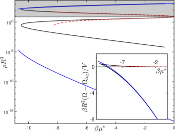
Figure 3: Maximum (in region with grey background) and minimum (white background) of $\rho$ as a function of $\beta\mu^{*}$ for the GEM-4 model in 3D, for FCC crystals. The inset shows the grand potential of the crystal minus that of the liquid per unit volume. The solid black lines are results from order 3 SNLT (including both the stable and unstable branches of solutions), red dashed lines resulting from a crystal approximation method Jiang and Si (2020) that uses Eq. (2), and the solid blue lines are obtained by using Eq. (1) to approximate the density distribution.

The reason for such remarkable efficiency of SNLT is that the convolution in (10) strongly damps modes with wavenumbers greater than some cut-off value (which depends on the particular system), as pointed out in Archer et al. (2019). The density $\rho=\rho_{0}\exp(\phi)$ is sharply peaked and so has large amplitudes over a wide range of Fourier modes, but when multiplied by $v(r)$ and averaged in the convolution, high wavenumber modes are damped. Of the three terms in (10), the last ($\beta\mu^{*}$) has only wavenumber zero, the second (convolution) term has only wavenumbers up to a cut-off, and so the first term $\phi({\bf r})$ can also only contain wavenumbers up to the same cut-off, and so can be represented accurately with relatively few Fourier modes. Thus, the logarithm of the sharply peaked density is a smooth function.

For the GEM-4 case, modes with wavenumbers $\gtrsim 2/R$ are strongly damped Archer et al. (2019), and (for crystals) SNLT of order 4 or higher includes only modes with wavenumbers above this cut-off (see the supplementary material Subramanian et al. (2021)), so order 3 SNLT is sufficient. The limited number of unknowns needed in SNLT makes it possible to determine crystal structures and compute phase diagrams using simple root finding packages (such as fsolve) or minimization packages in Matlab. Since the exact Eq. (7) has a similar structure to the approximate Eq. (10) – recall that all accurate DFTs are constructed from convolutions of the density with bounded functions (so-called weight functions) Evans (1992); Hansen and McDonald (2013); Roth (2010) – therefore the above argument that SNLT is accurate for periodic crystals because Fourier modes in $\ln\rho$ above a certain cut-off are strongly damped, applies in general, as long as the Fourier transform of the weight functions are short ranged. This is equivalent to the condition that the Fourier transform of $\int_{0}^{\lambda}\textrm{d}\lambda c^{(2)}({\bf r},{\bf r}^{\prime};\rho_{\lambda})$ [see (6)] becomes small beyond some cut-off. Thus, we expect SNLT to be widely applicable, not just to soft-core particles, although other systems may have the cut-off at larger $k$ than for GEM-4 model, requiring one to go a few orders higher for the SNLT to converge.

The efficiency of the truncated SNLT for crystals relies on the fact that there are a limited number of RLVs within the cut-off wavenumber. In contrast, the Fourier spectrum for QCs is dense Levine and Steinhardt (1984), and there is an infinite number of Fourier modes within any cut-off sphere. Including more modes in SNLT and/or using six-dimensional projection methods Jiang and Si (2020); Jiang et al. (2017); Jiang and Zhang (2018) turns out to be unsatisfactory because we get solutions only to a few digits of accuracy. Nonetheless, these provide good approximate initial conditions for other methods (such as Picard iteration used here), so we still advocate using the representation (3) and SNLT, combined with these other methods, for QCs.

We demonstrate this in a QC-forming system of soft particles interacting via the BEL pair potential Barkan et al. (2014); Ratliff et al. (2019)

$$v(r)=e^{-\frac{1}{2}\sigma^{2}r^{2}}\sum_{n=0}^{4}C_{2n}r^{2n}\,,$$ (11)

which was previously shown to form QCs in 2D Barkan et al. (2014); Ratliff et al. (2019). Here, we show that when the parameters $\{C_{2n},\sigma\}$ which control the form and range of $v(r)$ are chosen correctly, then this system also forms QCs in 3D. The values of $\{C_{2n},\sigma\}$ determine two characteristic lengthscales in the particle interactions, which we choose to be in the golden ratio $2\cos(\frac{\pi}{5})\approx 1.618$, in order to encourage IQCs Subramanian et al. (2016). We choose $\sigma$ to promote IQC stability whilst keeping $v(r)\geq 0$ for all $r$ Ratliff et al. (2019). Further details appear in the supplementary material Subramanian et al. (2021). To compute the phase diagram, we vary the coefficient $C_{6}$ in (11) and perform order 3 SNLT calculations for varying $\beta\mu^{*}$ ($C_{6}^{*}$ denotes the value at which the system is exactly marginally unstable at the two lengthscales). This is sufficient to accurately determine the periodic crystalline phases. However, for the IQC phase, we use the order 3 SNLT result as an initial condition for a Picard iteration solver Roth (2010); Hughes et al. (2014). Figure 4 displays the resulting phase diagram, which exhibits the liquid and two BCC crystals. The $q$-prefix denotes the crystal with lattice spacing determined by the smaller characteristic lengthscale (larger wavenumber). In between these two, the IQC emerges as the minimum of the grand potential $\Omega$. In parts of the region considered, the FCC structure is a local minimizer, but is never the global minimum. We have not calculated the free energy for all possible structures, but of the likely candidates, the IQC is the global minimum in a portion of the phase diagram.

Favourable contributions to $\Omega$ come from triangles and pentagons (combinations of three or five wavevectors that add up to zero) in the spectrum of $\rho$. Their abundance has been invoked to explain BCC (Alexander and McTague, 1978) and QC stability  (Bak, 1985; Mermin and Troian, 1985; Lifshitz and Diamant, 2007; Roan and Shakhnovich, 1998; Subramanian et al., 2016). However, the sharp peaks in $\rho$ and the consequential flatness of its spectrum obscures this argument. Our observation of strong damping at large $k$ in the spectrum of $\ln\rho$ suggests that the triangle argument should be reframed in terms of this field.

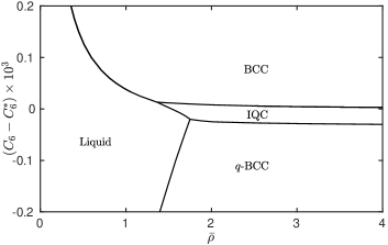
Figure 4: Phase diagram for the BEL system (11) in the average density $\bar{\rho}$ versus $C_{6}$ pair potential parameter plane. The IQC arises between the large lattice spacing BCC and small lattice spacing $q$-BCC. A liquid phase is also observed. The coexistence region between phases is of order the width of the lines.

In summary, we have demonstrated that SNLT, representing $\ln\rho$ as a truncated Fourier sum (3), is accurate at all state points, both near and far from melting. It is more efficient than representing $\rho$ as a Fourier sum (2), and it has a wider range of validity than representing it as a sum of Gaussians (1), which fails near melting and always predicts the density to be too low between the peaks. We expect SNLT to also be accurate for bicontinous and similar phases exhibited by e.g. the binary mixture considered in Pini et al. (2015). For QCs, we advocate SNLT as a method of generating good starting profiles for other (iterative) methods. Even without the SNLT severe truncation, in all cases we expect representation (3) to be superior to (2).