Abstract

A number of physical processes occurring in a flat one-dimensional graphene structure under the action of strong time-dependent electric fields are considered. It is assumed that the Dirac model can be applied to the graphene as a subsystem of the general system under consideration, which includes an interaction with quantized electromagnetic field. The Dirac model itself in the external electromagnetic field (in particular, the behavior of charged carriers) is treated nonperturbatively with respect to this field within the framework of strong-field QED with unstable vacuum. This treatment is combined with a kinetic description of the radiation of photons from the electron-hole plasma created from the vacuum under the action of the electric field. An interaction with quantized electromagnetic field is described perturbatively. A significant development of the kinetic equation formalism is presented. A number of specific results are derived in course of analytical and numerical study of the equations. We believe that some of predicted effects and properties of considered processes may be verified experimentally. Among these effects, it should be noted a characteristic spectral composition anisotropy of the quantum radiation and a possible presence of even harmonics of the external field in the latter radiation.

xx 1 5 Received: date; Accepted: date; Published: date Radiation problems accompanying carrier production by an electric field in the graphene Sergey P. Gavrilov ^1,3, Dmitry M. Gitman ^1,2,4, Vadim V. Dmitriev⁵, Anatolii D. Panferov⁵ and Stanislav A. Smolyansky^1,5* Firstname Lastname, Firstname Lastname and Firstname Lastname Correspondence: smol@info.sgu.ru 11.15.Tk; 78.67.Wj; 12.20.Ds

1 Introduction

Particle creation from the vacuum by strong electromagnetic and gravitational fields is a remarkable quantum effect predicted first in Refs. Klein (1929, 1927); Sauter (1931, 1931); Schwinger (1951) and studied then in Refs. Nikishov (1970, 1970, 1985); Narozhnyi (1970, 1974) in the framework of the relativistic quantum mechanics. Its exhaustive explanations and consistent nonperturbative methods of investigation became possible in the framework of quantum field theory (QFT). QFT with external backgrounds is, to a certain extent, an appropriate model for this purpose. In the framework of such a model, the particle creation is related to a violation of the vacuum stability. Backgrounds (external fields) that violate the vacuum stability are electric-like fields that are able to produce nonzero work when interacting with charged particles. Depending on the structure of such backgrounds, different approaches for calculating the effect were proposed and realized. From a quantum mechanical point of view, the most clear formulation of the problem of particle production from the vacuum by external fields is possible for time-dependent homogeneous external electric fields that are switched on and off at infinitely remote times $t\rightarrow\pm\infty$, respectively. Such kind of external fields are called $t$-electric potential steps ($t$-steps). Scattering, particle creation from the vacuum and particle annihilation by the $t$-steps were considered in the framework of the relativistic quantum mechanics, see Refs. Nikishov (1970, 1970, 1985); Narozhnyi (1970, 1974), a more complete list of relevant publications can be found in Refs. Ruffini (2010); Gelis (2016). A general nonperturbative with respect to the external background formulation of QED was developed in Ref. Gitman (1977); Fradkin (1981, 1991). In contrast to $t$-electric potential steps, there are many physically interesting situations where the external backgrounds are constant (time-independent) but spatially inhomogeneous, for example, concentrated in restricted space areas. The simplest type of such backgrounds are so-called $x$-electric potential steps ($x$-steps), in which the field is inhomogeneous only in one space direction and represents a spatial-like potential step for charged particles. The $x$-steps can also create particles from the vacuum, the Klein paradox is closely related to this process Klein (1929, 1927); Sauter (1931, 1931). Important calculations of the particle creation by $x$-steps in the framework of the relativistic quantum mechanics were presented in Refs. Nikishov (1970, 1970, 1985) and developed later in Refs. Hansen (1981). A general nonperturbative with respect to such external background formulation of QED was formulated in Ref. Gavrilov (2016). It is based on the existence of exact solutions of the Dirac or Klein-Gordon equation (wave equations, in what follows) with corresponding external fields. When such solutions can be found and all the calculations can be done analytically, we refer these examples as exactly solvable cases. Until now, there are known only few exactly solvable cases related to $t$-steps and to $x$-steps. In the case of $t$-steps, these are particle creation in a constant uniform electric field Schwinger (1951); Nikishov (1970, 1970, 1985), in an adiabatic electric field, Narozhnyi (1970, 1974), in the so-called $T$-constant electric field Bagrov (1975); Gavrilov (1996), in a periodic alternating in time electric field Narozhnyi (1970, 1974); Mostepanenko (1974), in an exponentially decaying electric field Adorno (2015), in an exponentially growing and decaying electric fields Adorno (2016, 2017) (see Ref. Adorno (2017) for the review), in a composite electric field Adorno (2018), and in an inverse-square electric field Adorno (2018). In the case of $x$-steps these are particle creation in the Sauter electric field Gavrilov (2016), in the so-called $L$-constant electric field Gavrilov (2016), and in the inhomogeneous exponential peak field Gavrilov (2017) and inverse-square electric field Adorno (2018, 2020).

Until recently, problems related to particle creation from the vacuum had mostly theoretical interest. This is related to the fact that the vacuum instability can be observed only in extremely strong external electric fields of the magnitude of $E_{c}=m^{2}/e\simeq 10^{16}V/cm$ ($E_{c}$ is the Schwinger’s critical field). However, recent technological advances in laser physics suggest that lasers such as those planned for the Extreme Light Infrastructure project (ELI) may be able to reach the nonperturbative regime of pair production in the near future (see review Dunne (2009)). Moreover, the situation has changed completely in recent years regarding applications to condensed matter physics: particle creation became an observable effect in graphene physics, an area which is currently under intense development Castro Neto (2009); Peres (2010); Vozmediano (2010); Das Sarma (2011). Briefly, this is explained by two facts: first, the low-energy electronic excitations in the graphene monolayer in the presence of an external electromagnetic field can be described by the Dirac model Semenoff (1984), namely, by a $2+1$ quantized Dirac field in such a background (here, dispersion surfaces are the so-called Dirac cones); and, second, the gap between the upper and lower branches in the corresponding Dirac particle spectra is very small, so that the particle creation effect turns out to be dominant (under certain conditions) as a response to the applied external electric-like field to the graphene. In particular, such an effect is crucial for understanding the conductivity in the graphene, specially in the so-called non-linear regime Allor (2008); Dóra (2010); Lewkowicz (2009); Rosenstein (2010); Kao (2010); Lewkowicz (2011). The first experimental observation of non-linear current-voltage characteristics ($I-V$) of graphene devices and its interpretation in terms of the pair-creation has been recently reported in Vandecasteele (2010). In the work Gavrilov (2012) the quantum electronic and energy transport in the graphene at low carrier density and low temperatures when quantum interference effects are important were studied in the framework of strong field QED. A formulation of the Dirac model in the Fock space that includes an interaction of photons with fermions was considered in Ref. Gavrilov (2016).

Due to a limited number of exactly solvable cases, approaches have been developed in parallel that make it possible, in the absence of appropriate exact solutions of the Dirac equation, to use certain approximate methods, including semiclassical and numerical, for nonperturbative calculations of quantum effects related to the vacuum instability. In this regard, it should be noted here the method of quantum kinetic equations (KE). In particular, this method is well adopted to using numerical calculations. In the framework of strong field QED, such an approach was also considered in Refs. Popov (1973); Grib (1934); Bialynicky-Birula (1991); Schmidt (1998); Kluger (1998); Mamaev (1979) (equivalence of the KE method and other exact methods was demonstrated in some cases in Refs. Dumlu (2009); Fedotov (2011)) and then applied to problems of QED with strong external fields (see, for example, Blaschke (2017)). This approach was recently adapted to the model of single-layer graphene in Smolyansky (2019); Panferov (2017); Smolyansky (2019).

In the present work we propose a generalization of the KE method taking into account an interaction of carriers with a photon reservoir in the graphene excited by an uniform, time-dependent electric field. It is assumed that the interaction of carriers with the external quasiclassical field is taken into account nonperturbatively, in contrast to their interaction with the quantized electromagnetic field. Thus, there appear collision integrals (CI) which take into account interaction with the quantized electromagnetic field in the single-photon approximation, corresponding to two channels: carrier redistribution by momenta as a result of a stimulated absorption or emission of photons and annihilation or creation of pairs. The kinetic description of these processes required the introduction of an appropriate KE for the photon subsystem. The Maxwell equations describing the generation of an internal plasma field close the system of equations.

In what follows, we restrict ourselves by the study of quantum radiation processes within the framework of the KE approach Blaschke (2011); Smolyansky (2019). We consider two different radiation mechanisms. One of them is a collective mechanism for the generation of plasma currents and waves (in the spatially uniform case, plasma oscillations Kluger (1998); Bloch (1999)). Corresponding electromagnetic fields can leave the region of active action of the external field and, as a result, can be detected far from it outside the graphene plane. In the graphene the excitation region is limited by a simply connected surface and it is not difficult to find the electromagnetic field in the whole space from surface currents Abbott (1985). A theoretical and experimental study of this kind of collective radiation was done in Refs. Baudisch (2018); Bowlan (2014) within the framework of an alternative dynamic approach Ishikava (2010, 2013) and in Smolyansky (2019) to the KE approach Smolyansky (2020). In addition to the above mentioned quasiclassical radiation, a quantum component of the radiation also exists due to elementary acts of interaction of the carriers with photons. In graphene, these mechanisms can be taken into account by analogy with the standard $D=3+1$ QED Blaschke (2011); Smolyansky (2019, 2020). Outside of the KE approach, this radiation mechanism was studied in Ref. Otto (2017). In the general case, these two mechanisms act self-consistent: the generation of the photon field leads to a back reaction problem of the second level, influencing plasma currents and oscillations of electromagnetic fields.

The approach considered in the present work is based on an adaptation of KE methods for a description of nonrelativistic plasma-like media in a nonequilibrium state (see, for example, deGroot (1980); Kadanoff (1962); Zubarev (1966)). The peculiarity of the system under consideration is that in the presence of external fields, massless quasiparticle states in the graphene are observed only indirectly and appear only through macroscopic characteristics, such as currents and the radiation, which are available for an observation during strongly nonequilibrium evolution at any time.  A more detailed discussion of the KE methods used in the present work and, in particular, the role of the polarization phenomena is given below in Sect. 5.

The work is organized as follows. In Subsect. 2.1 we briefly describe (following in main Refs. Panferov (2017); Smolyansky (2019, 2019, 2020)) a nonperturbative KE approach for studying evolution of carrier excitations in monolayer graphene under the action of an external quasiclassical time dependent electric field. The set of KE obtained here is an analog of the corresponding equations which was used in strong field QED (see, e.g. Blaschke (2017)). In the Subsect. 2.2 the KE are generalized to include the interaction of carriers with the quantized electromagnetic field. They allow us to consider a set of new problems: the radiation of the quantized field from the graphene, the photoproduction of carriers under the action of the quantized electromagnetic field, cascade processes, and so on. The obtained closed self-consistent system of KE appears as a result of an application of the truncation procedure of the Bogoliubov–Born–Green–Kirkwood–Yvon (BBGKY) chains of equations in the lower order of the perturbation theory with respect to the interaction of carriers with the photon reservoir. In the following Sect. 3 we set the problem how to consistently treat the radiation of the quantized electromagnetic field in the physical system under consideration. We argue that for our purposes it is enough to analyze only photon KE. The corresponding CI are quite complex functionals containing distribution functions of the carrier and photon subsystems. Significant simplifications appear in the case of a small photon density. This case we call the low density approximation. We note that, in addition, everywhere is used the long wave approximation. Some results obtained in the framework of such approximations are analyzed in Sect. 4. Then they are used in Sect. 5 in order to analyze the CI in the annihilation and the momentum redistribution channels. We also present parallel numerical estimates of some of the analytical results, and we are convinced of their qualitative coincidence. In Sect. 6 we present a summary of all obtained results, point out open problems, and outlook possible perspectives.

2 Kinetic equations describing quantum excitations in graphene placed in an electric field

2.1 Kinetic equations describing zero order processes

As was already mentioned in the Introduction, problems related to the vacuum instability can be studied in the framework the KE approach. Here we use such an approach to study the system of electronic excitations (charged carriers) and their interaction with electromagnetic fields in the graphene placed in an external electromagnetic field. Conditionally, the consideration is divided in two steps. On the first step, we consider production of the charged carriers from the quantum vacuum in the graphene under the action of a spatially uniform time-dependent external electric field $\mathbf{E}_{\mathrm{ext}}(t)=\left(E_{\mathrm{ext}}^{1}\left(t\right),E_{\mathrm{ext}}^{2}\left(t\right)\right)$ situated in the graphene plane $(x^{1},x^{2})$, distracting from a possible interaction of the carriers with the quantized electromagnetic field and neglecting possible modification of the external field due to a back reaction. According to terminology accepted in studying the vacuum instability, on this first step we consider KE approach for describing only zero order processes with respect to radiative corrections, see Ref. Gitman (1977); Fradkin (1981, 1991). On the second step, we take into account the interaction of the carriers with the quantized electromagnetic field, as well as with the modified due to the back reaction external field and then, on this base, we study the resulting electromagnetic field in the graphene. Partially, such a consideration takes into account the first order processes with respect to the radiative corrections. We stress that the first step consideration is based on KE approach describing zero order processes in the graphene placed in an external electric field and is nonperturbative with respect to the interaction with this field.

The external field is described by electromagnetic potentials $A_{\mathrm{ext}}^{\alpha}(t)$, $\alpha=1,2$. In the general case, the carriers in the graphene are subjected to an effective electric field,  

$$E^{\alpha}\left(t\right)=\ E_{\mathrm{ext}}^{\alpha}\left(t\right)+E_{\mathrm{int}}^{\alpha}\left(t\right),\;\alpha=1,2,$$ (1)

given by potentials

$$A^{\alpha}(t)=A_{\mathrm{ext}}^{\alpha}(t)+A_{\mathrm{int}}^{\alpha}(t),$$ (2)

where the internal field $E_{\mathrm{int}}^{\alpha}\left(t\right)$ is induced by a back-reaction mechanism (as will be shown, $E_{\mathrm{int}}\left(t\right)$ can be neglected under some suppositions). We let the electric field be switched on at $t_{\mathrm{in}}$ and switched off at $t_{\mathrm{out}}$, so that the interaction between the Dirac field and the electric field vanishes at all time instants outside the interval $t\in\left(t_{\mathrm{in}},t_{\mathrm{out}}\right)$.

To describe the carrier quantum motion we use the Dirac model of the graphene which describes the carries in a vicinity of one of the two Dirac points at boundaries of the Brillouin zone, see Refs. Novoselov (2005); Geim (2007); Castro Neto (2009) for a review. This model considers non interacting between themselves carriers placed in the external field. A wave function of a carrier is a two-component spinor $\psi(\mathbf{r},t)$. The latter satisfies the corresponding massless Dirac equation;

$$i\hbar\dot{\psi}(\mathbf{r},t)=h\left(t\right)\psi(\mathbf{r},t),\ h\left(t\right)={\mathrm{v}}_{F}\mathbf{\hat{P}}\left(t\right)\boldsymbol{\sigma},\ \mathbf{r}=\left(x^{1},x^{2}\right),$$ (3)

$$\mathbf{\hat{P}}\left(t\right)=\mathbf{\hat{p}}+\frac{e}{c}\mathbf{A}(t),\ e>0,\ \mathbf{\hat{p}}=-i\hbar\nabla\ .$$

The wave function $\psi(\mathbf{p},t)$ in the momentum representation is defined by the decomposition

$$\psi(\mathbf{r},t)=\frac{1}{\sqrt{S}}\sum_{\mathbf{p}}\psi(\mathbf{p},t)e^{i\mathbf{pr}/\hbar},$$ (4)

where $S$ is the area of the standard box regularization, and satisfies the following equation:

$$i\hbar\dot{\psi}\left(\mathbf{p},t\right)=h_{\mathbf{p}}\left(t\right)\psi\left(\mathbf{p},t\right),\;h_{\mathbf{p}}\left(t\right)={\mathrm{v}}_{F}{{\mathbf{P}}}\left(t\right){{\boldsymbol{\sigma}\ ,}}$$ (5)

whereas $\mathbf{P}$ is the kinetic momentum,

$$\mathbf{P}\left(t\right)=\mathbf{p}+\frac{e}{c}\mathbf{A}(t)=\left(P^{1},P^{2}\right).$$ (6)

Let us perform an unitary transformation $\psi\left(\mathbf{p},t\right)=U\left(t\right)\varphi\left(\mathbf{p},t\right),$ where the matrix $U$ has the form Dóra (2010):

$$U(t)=\frac{1}{\sqrt{2}}\left(\begin{array}[]{cc}\exp(-i\varkappa/2)&\exp(-i\varkappa/2)\\ \exp(i\varkappa/2)&-\exp(i\varkappa/2)\end{array}\right).$$ (7)

Then we come to an auxiliary quasienergy eigenvalue problem for the transformed Hamiltonian $\tilde{h}_{\mathbf{p}}(t)=U^{{\dagger}}(t)h_{\mathbf{p}}\left(t\right)U(t).$ We fix the parameter $\varkappa$ by the condition $\tan\varkappa=P^{2}/P^{1}$ such that the corresponding quasienergy (the excitation quasienergy or a dispersion law) is $\varepsilon(\mathbf{p},t)=\mathrm{v}_{F}\sqrt{\mathbf{P}^{2}}$ and:

$$\tilde{h}_{\mathbf{p}}(t)u_{\pm 1}=\pm\varepsilon(\mathbf{p},t)u_{\pm 1},\ u_{+1}=\left(\begin{array}[]{c}1\\ 0\end{array}\right),\ u_{-1}=\left(\begin{array}[]{c}0\\ 1\end{array}\right).$$ (8)

The spinor $\varphi\left(\mathbf{p},t\right)$ satisfies the equation

$$i\hbar\dot{\varphi}(\mathbf{p},t)=\tilde{h}_{\mathbf{p}}(t)\varphi(\mathbf{p},t)+\frac{1}{2}\lambda\hbar\sigma_{1}\varphi(\mathbf{p},t),$$ (9)

where the excitation function $\lambda(\mathbf{p},t)$ is determined from the equation $2iU^{\dagger}\dot{U}=\lambda\sigma_{1}$ and has the form:

$$\lambda(\mathbf{p},t)=\frac{ev_{F}^{2}[E_{\mathrm{ext}}^{1}(t)P^{2}-E_{\mathrm{ext}}^{2}(t)P^{1}]}{\varepsilon^{2}(\mathbf{p},t)}.$$ (10)

Note that the Dirac Hamiltonians $h\left(t\right)$ do not commute at distinct time instants, $\left[\tilde{h}_{\mathbf{p}}\left(t\right),\tilde{h}_{\mathbf{p}}\left(t^{\prime}\right)\right]\neq 0$ if $t\neq t^{\prime}$. In the model under consideration, the dispersion law holds true in a vicinity of the Dirac point $\mathbf{P}^{2}=0$ at the boundaries of the Brillouin zone. This model corresponds to low-energy excitations of the carries. However, the approach under consideration allows a generalization to a tight-binding model of the nearest neighbor interaction (see Refs. Castro Neto (2009); Kao (2010); Gusynin (2007)) as was demonstrated in Ref. Smolyansky (2019).

In which follows we are going to consider the so-called adiabatic ansatz (alternatively called the quasiparticle representation) which is widely used in semiclassical approximations and numeric calculations, see, e.g., Refs. Popov (1973); Bialynicky-Birula (1991); Schmidt (1998); Kluger (1998); Dumlu (2009); Fedotov (2011); Dabrowski (2014).

We recall that there are two species of fermions in the model, corresponding to excitations about two distinct Dirac points in the Brillouin zone, i.e., each of species belongs to a distinct valley. The algebra of $\gamma$-matrices has two inequivalent representations in $(2+1)$-dimensions and a distinct (pseudospin) representation is associated with each Dirac point. Another doubling of fields is due to the (real) spin of the electron. As a result, there are four species of fermions in the model. Thus, in order to find real mean values of physical quantities, one should to take into account the degeneracy factor $N_{f}=4$. We note that a transition to the quasiparticle representation in the model was used, for example, in Refs. Smolyansky (2019); Klimchitskaya (2013); Dóra (2010); Smolyansky (2020). Below we follow the works by Smolyansky (2019, 2020).

A quantum Dirac field ${\Psi(\mathbf{r},t)}$ associated with the function $\psi(\mathbf{r},t)$ satisfies Eq. (3) and the standard equal-time canonical anticommutation relations. It describes a fermion species of the model. The field operator $\Psi(\mathbf{p},t)$ in the momentum representation is defined by the decomposition:

$$\Psi(\mathbf{r},t)=\frac{1}{\sqrt{S}}\sum_{\mathbf{p}}\Psi(\mathbf{p},t)e^{i\mathbf{pr}/\hbar}\ .$$ (11)

Then it is convenient to introduce the field operator $\Phi(\mathbf{p},t)=U^{-1}\left(t\right)\Psi\left(\mathbf{p},t\right)$, which satisfies equation (9). According to the adiabatic ansatz, we define two kinds of creation and annihilation operators ($a^{\dagger}(\mathbf{p},t),a(\mathbf{p},t)$ and $b^{\dagger}(\mathbf{p},t),b(\mathbf{p},t)$) decomposing the operator $\Phi\left(\mathbf{p},t\right)$ into solutions $u_{\pm 1}$ (see Eq. (8)),

$$\Phi(\mathbf{p},t)=a(\mathbf{p},t)u_{+1}+b^{\dagger}(-\mathbf{p},t)u_{-1}\ .$$ (12)

Their nonzero anticommutation relations read:

$$\left[a(\mathbf{p},t),a^{\dagger}(\mathbf{p}^{\prime},t)\right]_{+}=\left[b(\mathbf{p},t),b^{\dagger}(\mathbf{p}^{\prime},t)\right]_{+}=\delta_{\mathbf{p,p}^{\prime}}\ .$$ (13)

In each time instant $t$, one can formally introduce a Fock space equipped by instantaneous vacuum vectors $|0,t\rangle,$

$$a(\mathbf{p},t)|0,t\rangle=b(\mathbf{p},t)|0,t\rangle=0,\ \forall\mathbf{p,}$$ (14)

and a corresponding basis originated by the action of the creation operators $a^{\dagger}(\mathbf{p},t)$ and $b^{\dagger}(\mathbf{p},t)$ on the corresponding vacuum vectors. Eq. (9) for the operator $\Phi\left(\mathbf{p},t\right)$ implies the following equations for the creation and annihilation operators:

$$i\hbar\dot{a}(\mathbf{p},t)=\varepsilon(\mathbf{p},t)a(\mathbf{p},t)-\frac{1}{2}\hbar\lambda(\mathbf{p},t)b^{\dagger}(-\mathbf{p},t),$$

$$i\hbar\dot{b}(-\mathbf{p},t)=\varepsilon(\mathbf{p},t)b(-\mathbf{p},t)+\frac{1}{2}\hbar\lambda(\mathbf{p},t)a^{\dagger}(-\mathbf{p},t).$$ (15)

The QFT Hamiltonian and the corresponding charge operator $Q$ in the model have the form:

$$H(t)=\int{d\mathbf{r}\Psi^{\dagger}(\mathbf{r},t)h\left(t\right)\Psi(\mathbf{r},t)\ ,}$$

$$Q(t)=-\frac{e}{2}\int{d\mathbf{r}}\left[{\Psi^{\dagger}(\mathbf{r},t),\Psi(\mathbf{r},t)}\right],\ {}$$ (16)

where the integration is over the finite area $S$. They can be diagonalized at any time instant $t$ using decomposition (12),

$$H(t)=\sum_{\mathbf{p}}\varepsilon(\mathbf{p},t)\left[a^{\dagger}(\mathbf{p},t)a(\mathbf{p},t)-b(-\mathbf{p},t)b^{\dagger}(-\mathbf{p},t)\right],$$

$$Q=-e\sum_{\mathbf{p}}\left[a^{\dagger}(\mathbf{p},t)a(\mathbf{p},t)-b^{\dagger}(-\mathbf{p},t)b(-\mathbf{p},t)\right].$$ (17)

The introduced above creation and annihilation operators become in- and out-operators of real quasiparticle at time instants $t_{\mathrm{in}}$ and $t_{\mathrm{out}}$ because the external electric field vanishes for $t\in\left(-\infty,t_{\mathrm{in}}\right)\cup\left(t_{\mathrm{out}},+\infty\right).$ They act in the corresponding Fock spaces with initial and final vacua $|0,\mathrm{in}\rangle=|0,t_{\mathrm{in}}\rangle$ and $|0,\mathrm{out}\rangle=|0,t_{\mathrm{out}}\rangle$ respectively. One interprets $a^{\dagger}(\mathbf{p},t_{\mathrm{in}})$ and $a(\mathbf{p},t_{\mathrm{in}})$ as creation and annihilation operators of initial electrons, $b^{\dagger}(\mathbf{p},t_{\mathrm{in}})$ and $b(\mathbf{p},t_{\mathrm{in}})$ as the creation and annihilation operators of initial holes, whereas $a^{\dagger}(\mathbf{p},t_{\mathrm{in}})a(\mathbf{p},t_{\mathrm{in}})$ and $b^{\dagger}(\mathbf{p},t_{\mathrm{in}})b(\mathbf{p},t_{\mathrm{in}})$ are operators of initial electron and hole numbers, respectively. Operators $a^{\dagger}(\mathbf{p},t_{\mathrm{out}})$ and $a(\mathbf{p},t_{\mathrm{out}})$ are interpreted as creation and annihilation operators of final electrons, $b^{\dagger}(\mathbf{p},t_{\mathrm{out}})$ and $b(\mathbf{p},t_{\mathrm{out}})$ as creation and annihilation operators of final holes, whereas $a^{\dagger}(\mathbf{p},t_{\mathrm{out}})a(\mathbf{p},t_{\mathrm{out}})$ and $b^{\dagger}(\mathbf{p},t_{\mathrm{out}})b(\mathbf{p},t_{\mathrm{out}})$ are interpreted as operators of final electron and hole numbers, respectively.

Since the particles are massless in the model under consideration, and spin degrees of freedom are hidden and manifest themselves only in the population of states, the charge is the only characteristic of the quasiparticles. It can be shown that the equation $\left[Q(t),H(t)\right]=0$ holds true at any time moment and, therefore, the electroneutrality of the system is preserved over time.

It is useful to introduce the following auxiliary distribution functions of quasiparticles (time-evolving adiabatic particle numbers)

$$f^{e}(\mathbf{p},t) = \langle 0,\mathrm{in}|a^{+}(\mathbf{p},t)a(\mathbf{p},t)|0,\mathrm{in}\rangle,$$ (18)

$$f^{h}(\mathbf{p},t) = \langle 0,\mathrm{in}|b^{+}(-\mathbf{p},t)b(-\mathbf{p},t)|0,\mathrm{in}\rangle.$$ (19)

Averaging charge operator (16) over the in-vacuum, and taking into account the charge conservation low, we obtain

$$f^{e}(\mathbf{p},t)=f^{h}(\mathbf{p},t)=f(\mathbf{p},t)\,.$$ (20)

Since $a(\mathbf{p},t_{\mathrm{in}})|0,\mathrm{in}\rangle=b(\mathbf{p},t_{\mathrm{in}})|0,\mathrm{in}\rangle=0,$ the initial value of the function $f(\mathbf{p},t)$ is zero, $f(\mathbf{p},t_{\mathrm{in}})=0$. When the electric field is turned off in an asymptotically distant future, the dispersion laws of quasiparticles goes to the mass surface,

$$\varepsilon_{\mathrm{out}}(\mathbf{p},t)=\mathrm{v}_{F}\sqrt{\left(\mathbf{p+}\frac{e}{c}\mathbf{A}_{\mathrm{out}}\right)^{2}},\ \mathbf{A}_{\mathrm{out}}=\lim_{t\rightarrow\infty}\mathbf{A}\left(t\right)\ .$$

Then functions (18) and (19) describe momentum distributions of real (observable) particles,

$$f(\mathbf{p},t_{\mathrm{out}})=\langle 0,\mathrm{in}|a^{+}(\mathbf{p},t_{\mathrm{out}})a(\mathbf{p},t_{\mathrm{out}})|0,\mathrm{in}\rangle=\langle 0,\mathrm{in}|b^{+}(\mathbf{p},t_{\mathrm{out}})b(\mathbf{p},t_{\mathrm{out}})|0,\mathrm{in}\rangle.$$ (21)

To get a closed set of KE, we differentiate $f(\mathbf{p},t)$ with respect to the time. Then using Eqs. (15) we obtain:

$$\dot{f}(\mathbf{p},t)=\frac{i\lambda\left(\mathbf{p},t\right)}{2}\left[f^{(+)}(\mathbf{p},t)-f^{(-)}(\mathbf{p},t)\right],$$ (22)

where the following anomalous expectation values

$$f^{(+)}(\mathbf{p},t)=\langle 0,\mathrm{in}|a^{+}(\mathbf{p},t)b^{+}(-\mathbf{p},t)|0,\mathrm{in}\rangle,$$

$$f^{(-)}(\mathbf{p},t)=\langle 0,\mathrm{in}|b(-\mathbf{p},t)a(\mathbf{p},t)|0,\mathrm{in}\rangle~{}$$ (23)

are introduced and $\lambda\left(\mathbf{p},t\right)$ is given by Eq. (10).

Time derivatives of the functions $f^{(\pm)}(\mathbf{p},t)$ have the form:

$$\dot{f}^{(+)}(\mathbf{p},t) = \frac{2i}{\hbar}\varepsilon(\mathbf{p},t)f^{(+)}(\mathbf{p},t)-\frac{i\lambda(\mathbf{p},t)}{2}[1-2f(\mathbf{p},t)],$$

$$\dot{f}^{(-)}(\mathbf{p},t) = \frac{-2i}{\hbar}\varepsilon(\mathbf{p},t)f^{(-)}(\mathbf{p},t)+\frac{i\lambda(\mathbf{p},t)}{2}[1-2f(\mathbf{p},t)].$$ (24)

As a result of the integration of these equations over time and substitution into Eq. (22), we obtain a KE of non-Markovian type in the following form:

$$\dot{f}(\mathbf{p},t)=I(\mathbf{p},t),$$

$$I(\mathbf{p},t)=\frac{1}{2}\lambda(\mathbf{p},t)\int_{t_{0}}^{t}\lambda(\mathbf{p},t^{\prime})[1-2f(\mathbf{p},t^{\prime})]\cos\theta(\mathbf{p};t,t^{\prime})dt^{\prime},$$ (25)

where the phase $\theta$ in the source function $I(\mathbf{p},t)$ reads:

$$\theta(\mathbf{p};t,t^{\prime})=\frac{2}{\hbar}\int_{t^{\prime}}^{t}dt^{\prime\prime}\varepsilon(\mathbf{p},t^{\prime\prime}).$$ (26)

The main task of the first stage is to find the distribution function $f\left(\mathbf{p},t\right)$ of created carriers. To this end it is convenient to introduce new functions $u(\mathbf{p},t)$ and $\nu(\mathbf{p},t)$ and reduce integro-differential Eq. (25) to an equivalent set of ordinary differential equations:

$$\dot{f}(\mathbf{p},t)=\frac{1}{2}\lambda(\mathbf{p},t)u(\mathbf{p},t),$$

$$\dot{u}(\mathbf{p},t)=\lambda(\mathbf{p},t)\left[1-2f(\mathbf{p},t)\right]-\frac{2\varepsilon(\mathbf{p},t)}{\hbar}\nu(\mathbf{p},t),\ \dot{\nu}(\mathbf{p},t)=\frac{2\varepsilon(\mathbf{p},t)}{\hbar}u(\mathbf{p},t).$$ (27)

The functions $u(\mathbf{p},t)$ and $\nu(\mathbf{p},t)$ describe polarization effects and are expressed in terms of anomalous means (23) as:

$$u(\mathbf{p},t)=f^{(+)}(\mathbf{p},t)+f^{(-)}(\mathbf{p},t),\ \nu(\mathbf{p},t)=i\left[f^{(+)}(\mathbf{p},t)-f^{(-)}(\mathbf{p},t)\right].$$ (28)

The total Hamiltonian of the fermion subsystem $H_{\mathrm{tot}}(t)=H(t)+H_{\mathrm{pol}}(t)$ contains two parts: the Hamiltonian $H(t)$ of the quasiparticle excitations (17) and a polarization Hamiltonian $H_{\mathrm{pol}}(t)$ which corresponds to the second term in the RHS of Eq. (9),

$$H_{\mathrm{pol}}(t)=-i\frac{\hbar}{2}\sum_{\mathbf{p}}\lambda(\mathbf{p},t)\left[a^{\dagger}(\mathbf{p},t)b^{\dagger}(-\mathbf{p},t)-b(-\mathbf{p},t)a(\mathbf{p},t)\right].$$ (29)

The corresponding vacuum polarization energy density can be represented as

$$E_{\mathrm{pol}}(t)=-\frac{\hbar}{2S}\sum_{\mathbf{p}}\lambda(\mathbf{p},t)v(\mathbf{p},t),$$ (30)

where $v(\mathbf{p},t)$is given by Eq. (28).

The vacuum mean value of the current density

$$\mathbf{j}(\mathbf{r},t)=\langle 0,\mathrm{in}|e{\mathrm{v}}_{F}\Psi^{\dagger}(\mathbf{r},t){\boldsymbol{\sigma}}\Psi(\mathbf{r},t)|0,\mathrm{in}\rangle$$

can be written in the following form:

$$\mathbf{j}\left(t\right)=\mathbf{j}_{\mathrm{cond}}\left(t\right)+\mathbf{j}_{\mathrm{pol}}\left(t\right),$$ (31)

see Smolyansky (2019, 2020). Here the conductivity $\mathbf{j}_{\mathrm{cond}}\left(t\right)$ and polarization current $\mathbf{j}_{\mathrm{pol}}\left(t\right)$ densities are:

$$j_{\mathrm{cond}}^{\alpha}\left(t\right) = \frac{2e}{S}\sum_{\mathbf{p}}v^{\alpha}(\mathbf{p},t)f(\mathbf{p},t)\ ,$$ (32)

$$j_{\mathrm{pol}}^{\alpha}\left(t\right) = -\frac{e}{S}\sum_{\mathbf{p}}\tilde{v}^{\alpha}(\mathbf{p},t)u(\mathbf{p},t)\ ,$$ (33)

where

$$v^{\alpha}(\mathbf{p},t)=\frac{\partial\varepsilon\left(\mathbf{p},t\right)}{\partial P^{\alpha}}=\frac{{\mathrm{v}}_{F}^{2}P^{\alpha}}{\varepsilon^{2}\left(\mathbf{p},t\right)}$$ (34)

is a group velocity and $\tilde{v}^{\alpha}(\mathbf{p},t)$ is the vector of the so-called conjugate velocity that is determined by components of vector (34) as follows: $\tilde{v}^{\alpha}(\mathbf{p},t)=\left(v^{2},-v^{1}\right)$. Note that the total current of all fermion species is $N_{f}\mathbf{j}\left(t\right)$. The role of current densities (32) and (33) in the electromagnetic emission in the graphene is discussed in Sect. 5.

The plasma classical electric field $\mathbf{E}_{\mathrm{int}}(t)$ is generated by the internal current $N_{f}\mathbf{j}\left(t\right)$ and satisfies the Maxwell equation,

$$\mathbf{\dot{E}}_{\mathrm{int}}(t)=-N_{f}\mathbf{j}\left(t\right).$$ (35)

This field contributes to the effective quasiclassical electric field (1) that in its turn has effect on the dynamics of carriers according to Eq. (27).

The above formulation of the quantum kinetic theory describing excitations in the graphene Smolyansky (2019, 2020) is constructed by analogy with the quantum kinetic theory describing the vacuum production of $e^{-}e^{+}$ plasma (see, e.g., Grib (1934); Blaschke (2009)).

In the thermodynamical limit $S\rightarrow\infty$, replacing the sum over the momenta in Eqs. (32) and (33) by an integral the conductivity and polarization current densities take the form

$$\mathbf{j}_{\mathrm{cond}}\left(t\right)=\frac{2e}{(2\pi\hbar)^{2}}\int\mathbf{v}(\mathbf{p},t)f(\mathbf{p},t)d\mathbf{p},$$ (36)

$$\mathbf{j}_{\mathrm{pol}}\left(t\right)=-\frac{e}{(2\pi\hbar)^{2}}\int\varepsilon(\mathbf{p},t)\mathbf{l}(\mathbf{p},t)u(\mathbf{p},t)d\mathbf{p},$$ (37)

where $\mathbf{v}(\mathbf{p},t)$ given by Eq. (34) is a propagation velocity of quasiparticle excitations, $\mathbf{l}(\mathbf{p},t)$ is a polarization function,

$$e\mathbf{l}(\mathbf{p},t)=(\partial\lambda(\mathbf{p},t)/\partial E_{\mathrm{ext}}^{1}\left(t\right),\ \partial\lambda(\mathbf{p},t)/\partial E_{\mathrm{ext}}^{2}\left(t\right)),$$

$$l_{1}(\mathbf{p},t)=v_{F}^{2}P_{2}/\varepsilon^{2}(\mathbf{p},t),\ l_{2}(\mathbf{p},t)=-v_{F}^{2}P_{1}/\varepsilon^{2}(\mathbf{p},t).$$ (38)

The function $\lambda(\mathbf{p},t)$ (10) can be expressed via $\mathbf{l}(\mathbf{p},t)$ as follows:

$$\lambda(\mathbf{p},t)=e\mathbf{E}_{\mathrm{ext}}(t)\mathbf{l}(\mathbf{p},t).$$ (39)

Thus, we see that polarization energy (30) and polarization current (37) are expressed in terms of polarization functions (28). We note that the separation of the total current in the sum of the conduction current and the polarization current is in a certain sense conditional but useful in approximate calculations.

Among the macroscopic averages it is necessary to refer also the number density of pairs of $N_{f}$ fermion species

$$n\left(t\right)=\frac{N_{f}}{(2\pi\hbar)^{2}}\int f(\mathbf{p},t)d\mathbf{p},$$ (40)

Following the works Grib (1934); Mamaev (1979), we can discover that for a finite $t$ the asymptotic behavior of solutions of system (27) for $\varepsilon(p,t)\rightarrow\infty$ is described by the following leading terms

$$f(\mathbf{p},t)\approx\frac{1}{16}\left(\frac{\lambda(\mathbf{p},t)}{\varepsilon(\mathbf{p},t)}\right)^{2},\;u(\mathbf{p},t)\approx\frac{1}{4\varepsilon(\mathbf{p},t)}\frac{d}{dt}\frac{\lambda(\mathbf{p},t)}{\varepsilon(\mathbf{p},t)},\;\nu(\mathbf{p},t)\approx\frac{\lambda(\mathbf{p},t)}{2\varepsilon(\mathbf{p},t)}\ .$$ (41)

Therefore, integrals (36), (37), and (40) converge. Note that for $t\rightarrow\infty$ the term (37) containing $u(p,t)$ vanishes because it is represented via an integral over momenta of a rapidly oscillating function. Assuming the external field being switched off for $t\rightarrow\infty$ the term $f(p,t)$ exponentially disappears with growth of $\varepsilon(p,t)$.

2.2 Inclusion an interaction with quantized electromagnetic field

Here we assume that excitations in the graphene interact both with effective classical electromagnetic field (2) and with the quantized electromagnetic field situated in the graphene plane. Below, we generalize the KE for such an extended system. The total QFT Hamiltonian $H_{\mathrm{tot}}(t)$ that corresponds to the system consists of a part which is originated from the Dirac model of excitations in the graphene interacting both with an external classical electromagnetic field and with the quantized electromagnetic field and of a Hamiltonian of the quantized electromagnetic field. Note that we consider explicitly an interaction with only one of a fermion species of the model. Thus, to find real mean values of physical quantities, one should to take into account the degeneracy factor $N_{f}=4$.

In the quasiparticle representation, introduced in Sect. 2.1, such a Hamiltonian reads:

$$H_{\mathrm{tot}}(t)=H(t)+H_{\mathrm{pol}}(t)+H_{\mathrm{int}}(t)+H_{\mathrm{A}}(t),$$ (42)

where Hamiltonians $H(t)$, given by Eq. (17), and $H_{\mathrm{pol}}(t)$ given by Eq. (28) describe excitations in the graphene and their interaction with existing in the graphene quasiclassical electromagnetic field $\mathbf{E}_{\mathrm{ext}}(t)$ whereas $H_{\mathrm{A}}(t)$ is a Hamiltonian of the free quantized electromagnetic field in the Coulomb gauge.

The electromagnetic field is not confined to the graphene surface, $z=0$, but rather propagates in the ambient $3+1$ dimensional space-time, where $z$ is the coordinate of axis normal to the graphene plane. We allow the graphene sheet to have a global momentum $p_{z}$ along the $z$ axis, in order to account for the possibility of a momentum transfer in this direction to some external system. However, only the projection of the electromagnetic field operator on the graphene plane $\mathbf{A}(x)=\left(A^{1}(x),A^{2}(x)\right)$ interacts with electrons and holes. Thus, we can exclude the noninteracting component, $A^{3}(x)$ of the electromagnetic field operator from the consideration and which corresponds to the case $z=0$. If the  wave vector of a photon field, $\left(k^{1},k^{2},k_{z}\right)$, has component $k_{z}\neq 0$ then the photon immediately leaves the interaction area. Such a free photon field can be represented with standard annihilation and creation operators and formulate in such terms a theory of emission in the first-order approximation with respect of electron-photon interaction Gavrilov (2016). However, in the present model we are interested in a different emission mechanism, which allows one to consider the photon field propagating along the graphene plane and having a sufficiently small momenta $k_{z}\rightarrow 0$. We chose the range of $k_{z}$ so as to emitted photon did not leave a graphene film of thickness $d$. Such a condition determines a limiting angle between the emission direction and the graphene plane,

$$\left|k_{z}\right|/k<\varphi,\;\varphi\sim d/\sqrt{S}\ll 1,$$ (43)

where $k=|\mathbf{k}|$ and $\mathbf{k}=\left(k^{1},k^{2}\right)$ is a two-component wave vector.

The operator of such a field can be written in the following form:

$$\hat{A}^{\alpha}(\mathbf{r},t)=\hat{A}^{(+)\alpha}(\mathbf{r},t)+\hat{A}^{(-)\alpha}(\mathbf{r},t),\ \alpha=1,2\ ,$$

$$\hat{A}^{(\pm)\alpha}(\mathbf{r},t)=\sqrt{\frac{\hbar c}{V}}\sum_{\mathbf{k}}\sum_{k_{z}<\varphi k}\frac{1}{\sqrt{2k}}\hat{A}^{(\pm)\alpha}(\pm\mathbf{k},k_{z},t)e^{-i\mathbf{kr}}\ ,$$

$$k=|\mathbf{k}|,\ \left[\hat{A}^{(\pm)\alpha}(\mathbf{k},k_{z},t)\right]^{{\dagger}}=A^{(\mp)\alpha}(-\mathbf{k},-k_{z},t)\ ,$$ (44)

where  $V=SL$ is the volume of the regularization box ($L$ is the length of the edge of the box normal to the graphene plane). This field is polarized and its polarization vector is transversal to the wavevector $\mathbf{k}$. The operators $\hat{A}^{(\pm)\alpha}(\mathbf{k},k_{z},t)$ satisfy standard equal time commutation relations:

$$\left[A^{(-)\alpha}(\mathbf{k},k_{z},t),A^{(+)\beta}(\mathbf{k}^{\prime},k_{z}^{\prime},t)\right] = \delta_{\alpha\beta}\delta_{\mathbf{kk}^{\prime}}\delta_{k_{z},k_{z}^{\prime}}\ ,$$

$$\left[A^{(\pm)\alpha}(\mathbf{k},k_{z},t),A^{(\pm)\beta}(\mathbf{k}^{\prime},k_{z}^{\prime},t)\right] = 0\ .$$ (45)

Then, the Hamiltonian $H_{\mathrm{A}}(t)$ of the free quantized electromagnetic field can be written as

$$H_{\mathrm{A}}(t)=c\hbar\sum_{\mathbf{k}}\sum_{k_{z}<\varphi k}k\hat{A}^{(+)\alpha}(\mathbf{k},k_{z},t)\hat{A}^{(-)\alpha}(\mathbf{k},k_{z},t),$$ (46)

The effective interaction of the carriers in graphene with the quantized electromagnetic field can be defined as: 

$$H_{\mathrm{int}}(t)=-e\frac{v_{F}}{c}\int d\mathbf{r}\Psi^{{\dagger}}(\mathbf{r},t){\boldsymbol{\sigma}}\Psi(\mathbf{r},t)\hat{\mathbf{A}}(\mathbf{r},t).$$ (47)

Substituting decompositions (11), (12) and (44) in Hamiltonian (47), we obtain:

$$\ H_{\mathrm{int}}(t)=-ev_{F}\sum_{\mathbf{p},\mathbf{k}}\sum_{k_{z}<\varphi k}\sqrt{\frac{\hbar}{2cVk}}\left\{\Gamma_{uu}^{\alpha}(\mathbf{p},\mathbf{p}-\hbar\mathbf{k};t)a^{{\dagger}}(\mathbf{p},t)a(\mathbf{p}-\hbar\mathbf{k},t)\right.$$

$$+\Gamma_{uv}^{\alpha}(\mathbf{p},\mathbf{p}-\hbar\mathbf{k};t)a^{{\dagger}}(\mathbf{p},t)b^{{\dagger}}(-\mathbf{p}+\hbar\mathbf{k},t)+\Gamma_{vu}^{\alpha}(\mathbf{p},\mathbf{p}-\hbar\mathbf{k};t)b(-\mathbf{p},t)a(\mathbf{p}-\hbar\mathbf{k},t)$$

$$+\left.\Gamma_{vv}^{\alpha}(\mathbf{p},\mathbf{p}-\hbar\mathbf{k};t)b(-\mathbf{p},t)b^{{\dagger}}(-\mathbf{p}+\hbar\mathbf{k},t)\right\}\hat{A}^{\alpha}(\mathbf{k},k_{z},t).$$ (48)

Here $\Gamma_{\xi\eta}^{\alpha}(\mathbf{p},\mathbf{p}^{\prime},t)$ are vertex matrix functions,

$$\Gamma_{\xi\eta}^{\alpha}(\mathbf{p},\mathbf{p}^{\prime},t)=\xi^{{\dagger}}U^{{\dagger}}(\mathbf{p},t)\sigma^{\alpha}U(\mathbf{p}^{\prime},t)\eta,\ \Gamma_{\xi\eta}^{\alpha\ast}(\mathbf{p},\mathbf{p}^{\prime};t)=\Gamma_{\eta\xi}^{\alpha}(\mathbf{p}^{\prime},\mathbf{p};t),$$ (49)

spinors $\xi$ and $\eta$ are given by Eqs. (8), and the evolution matrix $U(\mathbf{p},t),$ which describes the influence of the external field on the interaction of the introduced quasiparticles with photons is given by Eq. (7).

Hamiltonian (42), being written in the quasiparticle representation, determines the time evolution of creation and annihilation operators of all the particles,

$$\dot{a}(\mathbf{p},t)=-\frac{i}{\hbar}\varepsilon(\mathbf{p},t)a(\mathbf{p},t)+\frac{i}{2}\lambda(\mathbf{p},t)b^{{\dagger}}(-\mathbf{p},t)+ev_{F}\sum_{\mathbf{k}}\sum_{k_{z}<\varphi k}\frac{i}{\sqrt{2\hbar cVk}}$$

$$\times\left\{\Gamma_{uu}^{\alpha}(\mathbf{p},\mathbf{p}^{\prime};t)a(\mathbf{p}-\hbar K,t)+\Gamma_{uv}^{\alpha}(\mathbf{p},\mathbf{p}^{\prime};t)b^{{\dagger}}(-\mathbf{p}^{\prime},t)\right\}\hat{A}^{\alpha}(\mathbf{k},k_{z},t),$$

$$\dot{b}(-\mathbf{p},t)=-\frac{i}{\hbar}b(-\mathbf{p},t)-\frac{i}{2}\lambda(\mathbf{p},t)a^{{\dagger}}(\mathbf{p},t)-ev_{F}\sum_{\mathbf{k}}\sum_{k_{z}<\varphi k}\frac{i}{\sqrt{2\hbar cVk}}$$

$$\times\left\{\Gamma_{uv}^{\alpha}(\mathbf{p}+\hbar K,\mathbf{p};t)a^{{\dagger}}(\mathbf{p}+\hbar\mathbf{k},t)+\Gamma_{vv}^{\alpha}(\mathbf{p}+\hbar K,\mathbf{p};t)b(-\mathbf{p}^{\prime},t)\right\}\hat{A}^{\alpha}(\mathbf{k},k_{z},t),$$

$$\dot{\hat{A}}^{(\pm)\alpha}(\pm\mathbf{k},k_{z},t)=\pm iK\mathcal{A^{(\pm)\alpha}}(\pm\mathbf{k},k_{z},t)\mp ev_{F}\sum_{\mathbf{p}}\frac{i}{\sqrt{2\hbar cVk}}$$

$$\left\{\Gamma_{uu}^{\alpha}(\mathbf{p},\mathbf{p}^{\prime};t)a^{{\dagger}}(\mathbf{p},t)a(\mathbf{p}^{\prime},t)+\Gamma_{uv}^{\alpha}(\mathbf{p},\mathbf{p}^{\prime};t)a^{{\dagger}}(\mathbf{p},t)b^{{\dagger}}(-\mathbf{p}^{\prime},t)\right.$$

$$+\left.\Gamma_{vu}^{\alpha}(\mathbf{p},\mathbf{p}^{\prime};t)b(-\mathbf{p},t)a(\mathbf{p}^{\prime},t)+\Gamma_{vv}^{\alpha}(\mathbf{p},\mathbf{p}^{\prime};t)b(-\mathbf{p},t)b^{{\dagger}}(-\mathbf{p}^{\prime},t)\right\},$$ (50)

where $\mathbf{p}^{\prime}\mathbf{=p-\hbar k}$.

Now we introduce the correlation function $f(\mathbf{p},\mathbf{p}\,^{\prime};t)$ of the electron-hole subsystem and the one $F_{\alpha\beta}(\mathbf{k},\mathbf{k}\,^{\prime};t)$ of the photon subsystem,

$$f(\mathbf{p},\mathbf{p}\,^{\prime};t)=\langle 0,\mathrm{in}|a^{{\dagger}}(\mathbf{p},t)a(\mathbf{p}\,^{\prime},t)|0,\mathrm{in}\rangle,$$

$$F_{\alpha\beta}(\mathbf{k},\mathbf{k}\,^{\prime};t)=\sum_{k_{z}<\varphi k}\langle 0,\mathrm{in}|\hat{A}^{(+)\alpha}(\mathbf{k},k_{z},t)\hat{A}^{(-)\beta}(\mathbf{k}\,^{\prime},k_{z}^{\prime},t)|0,\mathrm{in}\rangle.$$ (51)

In the case of spatially-homogeneous systems the correlation functions, being written in the coordinate representation, depend on the coordinate difference only. Their Fourier transforms depend of the corresponding $\delta$ functions. Note that under the condition $\varphi\rightarrow 0$ the momentum distribution of photons does not depend on $k_{z}$ and the correlation function $F_{\alpha\beta}(k,k\,^{\prime};t)$ is simply proportional to the number of state with $k_{z}<\varphi k$, $n\left(k\right)=\frac{kd}{2\pi}$. Thus, the correlation functions (51) have the form:

$$f(\mathbf{p},\mathbf{p}^{\prime};t)=f(\mathbf{p},t)\frac{S}{\left(2\pi\right)^{2}}\delta_{\mathbf{p},\mathbf{p}^{\prime}}\ ,$$ (52)

$$F_{\alpha\beta}(\mathbf{k},\mathbf{k}^{\prime};t)=F(\mathbf{k},t)n\left(k\right)\frac{S}{\left(2\pi\right)^{2}}\delta_{\alpha\beta}\delta_{\mathbf{k},\mathbf{k}^{\prime}\ },$$ (53)

where

$$F(\mathbf{k},t)=\frac{1}{2}\sum_{\alpha}F_{\alpha\alpha}(\mathbf{k},\mathbf{k}^{\prime};t)|_{\mathbf{k}^{\prime}=\mathbf{k}\ }.$$ (54)

In Eq. (52) $f(\mathbf{p},t)$ is  a superficial density of electron (hole) numbers with a momentum $\mathbf{p}$ at the time instant $t,$ whereas $F(\mathbf{k},t)$ in Eq. (53) is a superficial density of photons with the wave vector $\mathbf{k}$ at the time instant $t$ per unit state with a given $k_{z}$. In which follows, we use the notation $\hat{A}^{\alpha}(k,t)=\hat{A}^{\alpha}(k,0,t)$ for the photon operator with a given $k_{z}\rightarrow 0$   .

Eqs. (50) imply the following equations for the introduced distribution functions:

$$\dot{f}(\mathbf{p},t)=\frac{1}{2}\lambda(\mathbf{p},t)u(\mathbf{p},t)-iev_{F}\sum_{\mathbf{k}}\frac{(2\pi)^{2}n\left(k\right)}{\sqrt{2\hbar cVk}}$$

$$\times\left\{\Gamma_{uu}^{\alpha\ast}(\mathbf{p},\mathbf{p}-\hbar\mathbf{k};t)\langle 0,\mathrm{in}|a^{{\dagger}}(\mathbf{p}-\hbar\mathbf{k},t)a(\mathbf{p},t)\hat{A}^{\alpha}(\mathbf{k},t)|0,\mathrm{in}\rangle\right.$$

$$+\Gamma_{uv}^{\alpha\ast}(\mathbf{p},\mathbf{p}-\hbar\mathbf{k};t)\langle 0,\mathrm{in}|b(-\mathbf{p}+\hbar\mathbf{k},t)a(\mathbf{p},t)\hat{A}^{\alpha}(\mathbf{k},t)|0,\mathrm{in}\rangle$$

$$-\Gamma_{uu}^{\alpha}(\mathbf{p},\mathbf{p}-\hbar\mathbf{k};t)\langle 0,\mathrm{in}|a^{{\dagger}}(\mathbf{p},t)a(\mathbf{p}-\hbar\mathbf{k},t)\hat{A}^{\alpha}(\mathbf{k},t)|0,\mathrm{in}\rangle$$

$$-\left.\Gamma_{uv}^{\alpha}(\mathbf{p},\mathbf{p}-\hbar\mathbf{k};t)\langle 0,\mathrm{in}|a^{{\dagger}}(\mathbf{p},t)b^{{\dagger}}(-\mathbf{p}-\hbar\mathbf{k},t)\hat{A}^{\alpha}(\mathbf{k},t)|0,\mathrm{in}\rangle\right\},$$ (55)

and

$$\dot{F}(\mathbf{k},t)=-iev_{F}\sum_{\mathbf{p}}\frac{2\pi^{2}}{\sqrt{\hbar cVk}}\left\{\Gamma_{uu}^{\alpha}(\mathbf{p},\mathbf{p}+\hbar\mathbf{k};t)\langle 0,\mathrm{in}|a^{{\dagger}}(\mathbf{p},t)a(\mathbf{p}+\hbar\mathbf{k},t)\hat{A}^{(-)\alpha}(\mathbf{k},t)|0,\mathrm{in}\rangle\right.$$

$$+\Gamma_{uv}^{\alpha}(\mathbf{p},\mathbf{p}+\hbar\mathbf{k};t)\langle 0,\mathrm{in}|a^{{\dagger}}(\mathbf{p},t)b^{{\dagger}}(-\mathbf{p}-\hbar\mathbf{k},t)\hat{A}^{(-)\alpha}(\mathbf{k},t)|0,\mathrm{in}\rangle$$

$$+\Gamma_{vu}^{\alpha}(\mathbf{p},\mathbf{p}+\hbar\mathbf{k};t)\langle 0,\mathrm{in}|b(-\mathbf{p},t)a(\mathbf{p}+\hbar\mathbf{k},t)\hat{A}^{(-)\alpha}(\mathbf{k},t)|0,\mathrm{in}\rangle$$

$$+\Gamma_{vv}^{\alpha}(\mathbf{p},\mathbf{p}+\hbar\mathbf{k};t)\langle 0,\mathrm{in}|b(-\mathbf{p},t)b^{{\dagger}}(-\mathbf{p}-\hbar\mathbf{k},t)\hat{A}^{(-)\alpha}(\mathbf{k},t)|0,\mathrm{in}\rangle$$

$$-\Gamma_{uu}^{\alpha}(\mathbf{p},\mathbf{p}-\hbar\mathbf{k};t)\langle 0,\mathrm{in}|\hat{A}^{(+)\alpha}(\mathbf{k},t)a^{{\dagger}}(\mathbf{p},t)a(\mathbf{p}-\hbar\mathbf{k},t)|0,\mathrm{in}\rangle$$

$$-\Gamma_{uv}^{\alpha}(\mathbf{p},\mathbf{p}-\hbar\mathbf{k};t)\langle 0,\mathrm{in}|\hat{A}^{(+)\alpha}(\mathbf{k},t)a^{{\dagger}}(\mathbf{p},t)b^{{\dagger}}(-\mathbf{p}+\hbar\mathbf{k},t)|0,\mathrm{in}\rangle$$

$$-\Gamma_{vu}^{\alpha}(\mathbf{p,p}-\hbar\mathbf{k};t)\langle 0,\mathrm{in}|\hat{A}^{(+)\alpha}(\mathbf{k},t)b(-\mathbf{p},t)a(p-\hbar\mathbf{k},t)|0,\mathrm{in}\rangle$$

$$-\left.\Gamma_{vv}^{\alpha}(\mathbf{p},\mathbf{p}-\hbar\mathbf{k};t)\langle 0,\mathrm{in}|\hat{A}^{(+)\alpha}(\mathbf{k},t)b(-\mathbf{p},t)b^{{\dagger}}(-\mathbf{p}+\hbar\mathbf{k},t)|0,\mathrm{in}\rangle\right\}.$$ (56)

Equation (55) reduces to the first equation of set (27) when the electron-hole system does not interact with photons

The system of Eqs. (55) and (56) is not closed, their RHS contain higher order correlation functions. The means $\langle 0,\mathrm{in}|a^{{\dagger}}a\hat{A}^{(\pm)}|0,\mathrm{in}\rangle$ and $\langle 0,\mathrm{in}|b^{{\dagger}}b\hat{A}^{(\pm)}|0,\mathrm{in}\rangle$ correspond to processes of induced irradiation and absorption, whereas the means $\langle 0,\mathrm{in}|ab\hat{A}^{(+)}|0,\mathrm{in}\rangle$ and $\langle 0,\mathrm{in}|a^{{\dagger}}b^{{\dagger}}\hat{A}^{(-)}|0,\mathrm{in}\rangle$ correspond to processes with pair annihilation and creation. We do not consider the phantom process with the correlators $\langle 0,\mathrm{in}|a^{{\dagger}}b^{{\dagger}}\hat{A}^{(+)}|0,\mathrm{in}\rangle$ and $\langle 0,\mathrm{in}|ab\hat{A}^{(-)}|0,\mathrm{in}\rangle$.

Equations (55) and (56) constitute a part of the Bogoliubov–Born–Green–Kirkwood–Yvon (BBGKY) chain of equations in the electron-hole and photon sectors. To close the set (55) and (56) it is necessary to obtain equations of the second level for all the above mentioned correlation functions. These equations will already contain two-particle correlation functions, which, assuming a weak interaction between the subsystems, can again be represented through the single-particle correlator.

Below we give an example of a truncation procedure:

$$\ \langle 0,\mathrm{in}|a^{{\dagger}}(\mathbf{p}_{1},t)a(\mathbf{p}_{2},t)\hat{A}_{\beta}(\mathbf{k}\,^{\prime},t)\hat{A}_{\alpha}^{(\pm)}(\mathbf{k},t)|0,\mathrm{in}\rangle=\frac{S^{2}}{\left(2\pi\right)^{4}}f(\mathbf{p}_{1},t)\delta_{\mathbf{p}_{1},\mathbf{p}_{2}}\delta_{\alpha\beta}\left\{\begin{array}[]{c}\left[F(\mathbf{k},t)+1\right]\delta_{\mathbf{k},-\mathbf{k}^{\prime}}\\ F(\mathbf{k},t)\delta_{\mathbf{k},\mathbf{k}^{\prime}}\end{array}\right.,$$ (60)

$$\langle 0,\mathrm{in}|a^{{\dagger}}(\mathbf{p}_{1},t)a(\mathbf{p}_{2},t)a^{{\dagger}}(\mathbf{p}\,^{\prime},t)a(\mathbf{p}\,^{\prime\prime},t)|0,\mathrm{in}\rangle$$

$$= \frac{S^{2}}{\left(2\pi\right)^{4}}f(\mathbf{p}_{1},t)\left[f(\mathbf{p}^{\prime},t)\delta_{\mathbf{p}_{1},\mathbf{p}_{2}}\delta_{\mathbf{p}^{\prime},\mathbf{p}^{\prime\prime}}+\left[1-f(\mathbf{p}^{\prime},t)\right]\delta_{\mathbf{p}_{1},\mathbf{p}^{\prime\prime}}\delta_{\mathbf{p}_{2},\mathbf{p}^{\prime}}\right],$$

$$\ \langle 0,\mathrm{in}|a^{{\dagger}}(\mathbf{p}_{1},t)a(\mathbf{p}_{2},t)b(-\mathbf{p}^{\prime},t)b^{{\dagger}}(-\mathbf{p}^{\prime\prime},t)|0,\mathrm{in}\rangle=\frac{S^{2}}{\left(2\pi\right)^{4}}f(\mathbf{p}_{1},t)\left[1-f(\mathbf{p}^{\prime},t)\right]\delta_{\mathbf{p}_{1},\mathbf{p}_{2}}\delta_{\mathbf{p}^{\prime},\mathbf{p}^{\prime\prime}}\ .$$

It corresponds to the random-phase-approximation (RPA) Kadanoff (1962); Zubarev (1966). We note that in the truncation procedure one neglects polarization effects in the resulting CI and in the evolution equations for the polarization functions $u(\mathbf{p},t)$ and $v(p,t)$ (27). Here, the assumption of spatial homogeneity and its consequence (51) were taken into account.

In such a way, a closed set of equations for the distribution functions $f(\mathbf{p},t)$ and $F(\mathbf{k},t)$ can be obtained. In the thermodynamic limit $V\rightarrow\infty$ it reads:

$$\dot{f}(\mathbf{p},t) = I(\mathbf{p},t)+C_{\gamma}(\mathbf{p},t)+C_{\mathrm{eh}}(\mathbf{p},t)\ ,$$ (61)

$$\dot{F}(\mathbf{k},t) = S_{\gamma}(\mathbf{k},t)+S_{\mathrm{eh}}(\mathbf{k},t).$$ (62)

Collision integrals $C_{\gamma}(\mathbf{p},t)$ and $C_{\mathrm{eh}}(\mathbf{p},t)$ that describe creation and annihilation of $\mathrm{eh}$-pairs or a distribution of carries in momenta in course of one-photon absorption or emission respectively have the form:

$$C_{\gamma}(\mathbf{p},t)=2\int\frac{d\mathbf{k}n\left(k\right)}{\left(2\pi\hbar\right)^{2}}\int_{t_{0}}^{t}dt^{\prime}K_{\gamma}(\mathbf{p},\mathbf{p}+\hbar\mathbf{k};t,t^{\prime})$$

$$\left\{f(\mathbf{p},t^{\prime})f(\mathbf{p}+\hbar\mathbf{k},t^{\prime})[1+F(\mathbf{k},t^{\prime})]-[1-f(\mathbf{p},t^{\prime})][1-f(\mathbf{p}+\hbar\mathbf{k},t^{\prime})]F(\mathbf{k},t^{\prime})\right\}$$ (63)

$$C_{\mathrm{eh}}(\mathbf{p},t)=2\int\frac{d\mathbf{k}n\left(k\right)}{\left(2\pi\hbar\right)^{2}}\int_{t_{0}}^{t}dt^{\prime}K_{\mathrm{eh}}(\mathbf{p},\mathbf{p}+\hbar\mathbf{k};t,t^{\prime})$$

$$\left\{f(\mathbf{p},t^{\prime})[1-f(\mathbf{p}+\hbar\mathbf{k},t^{\prime})][1+F(\mathbf{k},t^{\prime})]-f(\mathbf{p},t^{\prime})[1-f(\mathbf{p}+\hbar\mathbf{k},t^{\prime})]F(\mathbf{k},t^{\prime})\right\}.$$ (64)

Collision integrals in the photon sector read:

$$S_{\gamma}(\mathbf{k},t)=2\int\frac{d\mathbf{p}}{\left(2\pi\hbar\right)^{2}}\int_{t_{0}}^{t}dt^{\prime}K_{\gamma}(\mathbf{p},\mathbf{p}+\hbar\mathbf{k};t,t^{\prime})$$

$$\left\{f(\mathbf{p},t^{\prime})f(\mathbf{p}+\hbar\mathbf{k},t^{\prime})[1+F(\mathbf{k},t^{\prime})]-[1-f(\mathbf{p},t^{\prime})][1-f(\mathbf{p}+\hbar\mathbf{k},t^{\prime})]F(\mathbf{k},t^{\prime})\right\}$$ (65)

$$S_{\mathrm{eh}}(\mathbf{k},t)=2\int\frac{d\mathbf{p}}{\left(2\pi\hbar\right)^{2}}\int_{t_{0}}^{t}dt^{\prime}K_{\mathrm{eh}}(\mathbf{p},\mathbf{p}+\hbar\mathbf{k};t,t^{\prime})$$

$$\left\{f(\mathbf{p},t^{\prime})[1-f(\mathbf{p}+\hbar\mathbf{k},t^{\prime})][1+F(\mathbf{k},t^{\prime})]-f(\mathbf{p},t^{\prime})[1-f(\mathbf{p}+\hbar\mathbf{k},t^{\prime})]F(\mathbf{k},t^{\prime})\right\}.$$ (66)

We note that kernels in collision integrals (63)-(66) in the photon and $\mathrm{eh}$-sectors are the same and have the form:

$$K_{\gamma}(\mathbf{p},\mathbf{p}+\hbar\mathbf{k};t,t^{\prime})=\frac{(ev_{F})^{2}}{2\hbar ck}\Gamma_{uv}^{\alpha}(\mathbf{p},\mathbf{p}+\hbar\mathbf{k};t)\Gamma_{uv}^{\alpha\ast}(\mathbf{p},\mathbf{p}+\hbar\mathbf{k};t^{\prime})\cos\Theta^{(+)}(\mathbf{p},\mathbf{p}+\hbar\mathbf{k};t,t^{\prime}),$$

$$K_{\mathrm{eh}}(\mathbf{p},\mathbf{p}+\hbar\mathbf{k};t,t^{\prime})=\frac{(ev_{F})^{2}}{2\hbar ck}\Gamma_{uu}^{\alpha}(\mathbf{p},\mathbf{p}+\hbar\mathbf{k};t)\Gamma_{uu}^{\alpha\ast}(\mathbf{p},\mathbf{p}+\hbar\mathbf{k};t^{\prime})\cos\Theta^{(-)}(\mathbf{p},\mathbf{p}+\hbar\mathbf{k};t,t^{\prime}),$$

$$\Theta^{(\pm)}(\mathbf{p},\mathbf{p}+\hbar\mathbf{k};t,t^{\prime})=\frac{1}{\hbar}\int_{t^{\prime}}^{t}d\tau\left[\varepsilon(\mathbf{p},\tau)\pm\varepsilon(\mathbf{p}+\hbar\mathbf{k},\tau)-c\hbar k\right].$$ (67)

This fact allows one to interpret collision integrals (63), (64) and (65), (66) as a reduction of some unified integrands to the photon and $\mathrm{eh}$-sectors.

3 Setting of the problem

The set of KE (61) and (62) with CI (63)-(66) and Maxwell equations (35) describe a self-consistent dynamics of carriers in the graphene and a behavior of the internal electromagnetic fields. The same set of equations describes an electromagnetic radiation from graphene, both classical, generated by plasma currents, and quantum, due to one-photon processes. Since the classical radiation has already been studied on the basis of KE, see Baudisch (2018); Bowlan (2014), in the present work we focus our attention on the quantum radiation, in particular, comparing its characteristics with the once of the classical radiation. Below, we study this problem solving photon KE (62). This corresponds to neglecting the back reaction of the quantum radiation on carrier dynamics, which is still being described by Eq. (25) but with effective external field (1). Thus, the action of the photon subsystem on the evolution of the $\mathrm{eh}$ subsystem and the cascade processes remains outside the scope of this study, as well as the action of the quantum radiation on effective electric field (1).

In order to solve the problem, we rewrite Eqs. (65) and (66), neglecting the influence of the photon subsystem,

$$S_{\gamma}(\mathbf{k},t)=\frac{2}{\left(2\pi\hbar\right)^{2}}\int d\mathbf{p}\int_{t_{0}}^{t}dt^{\prime}K_{\gamma}\left(\mathbf{p,p+}\hbar\mathbf{k};t,t^{\prime}\right)f(\mathbf{p},t^{\prime})f\left(\mathbf{p+}\hbar\mathbf{k,}t^{\prime}\right),$$ (68)

$$S_{\mathrm{eh}}(\mathbf{k},t)=\frac{2}{\left(2\pi\hbar\right)^{2}}\int d\mathbf{p}\int_{t_{0}}^{t}dt^{\prime}K_{\mathrm{eh}}\left(\mathbf{p,p+}\hbar\mathbf{k};t,t^{\prime}\right)f(\mathbf{p},t^{\prime})\left[1-f(\mathbf{p+}\hbar\mathbf{k},t^{\prime})\right].$$ (69)

Thus, at this stage, we study Eq. (62) with CI (68) and (69) that do not contain the photon distribution function. We take into account only a spontaneous emission from the carrier currents produced by an external electric field. Integrals (68) and (69) contain quadratic combinations of the distribution functions of the carriers. These functions should be found as a result of solving an auxiliary problem on the basis of KE (25) or equivalent equations (27).

4 Studying processes in specific external fields

4.1 Models of external fields

Below, we study the KE that describe the behavior of the carriers and the electromagnetic field in the graphene when external field is linearly polarized, $A_{\mathrm{ext}}^{1}=0$ ($E_{\mathrm{ext}}^{1}=0$). Two following models of the linear polarized short laser pulse Hebenstreit (2009) are convenient for numerical modelling of the CI (68) and (69). First we consider the two following potentials $A_{\mathrm{ext}}^{2}(t)$ and corresponding fields $E_{\mathrm{ext}}^{2}(t)$:

$$A_{\mathrm{ext}}^{2}(t)=A_{c}(t)=-\sqrt{\frac{\pi}{8}}E_{0}\tau\exp(-\sigma^{2}/2){\mathrm{erf}}\left(\frac{t}{\sqrt{2\tau}}-i\frac{\sigma}{\sqrt{2}}\right)+c.c.\ ,$$

$$E_{\mathrm{ext}}^{2}(t)=E_{c}(t)=E_{0}\exp(-t^{2}/2\tau^{2})\cos\omega t,\ \sigma=\omega\tau\ ,\ \sigma=\omega\tau\ ,$$ (70)

and

$$A_{\mathrm{ext}}^{2}(t) = A_{s}(t)=i\sqrt{\frac{\pi}{8}}E_{0}\tau\exp(-\sigma^{2}/2)\mathrm{erf}\left(\frac{t}{\sqrt{2\tau}}-i\frac{\sigma}{\sqrt{2}}\right)-c.c.\ ,$$

$$E_{\mathrm{ext}}^{2}(t) = E_{s}(t)=E_{0}\exp(-t^{2}/2\tau^{2})\sin\omega t\ ,$$ (71)

where $\mathrm{erf}\left(x\right)$ is the error function, $\omega=2\pi/T$ is the cyclic frequency and $\tau$ is the envelope pulse length.

We are going also to use a model of a harmonic electric field in some analytical calculations:

$$A_{\mathrm{ext}}^{2}(t)=A(t)=-(E_{0}/\omega)\sin\omega t,\ E_{\mathrm{ext}}^{2}(t)=E(t)=E_{0}\cos\omega t\ .$$ (72)

4.2 Low-density approximation

Below, to analyze CI (68) and (69) by analytical methods we introduce some approximations for basic constituents of these CI.

In order to estimate of the distribution function, we will use the low-density approximation $f(\mathbf{p},t)\ll 1$ Fedotov (2011), which immediately allows one to write a solution with the zero initial date $f(t_{0})=0$ of Eqs. (25) - (26) as:

$$f(t)=\frac{1}{2}\int_{t_{0}}^{t}dt^{\prime}\lambda(t^{\prime})\int_{t_{0}}^{t^{\prime}}dt^{\prime\prime}\lambda(t^{\prime\prime})\cos\theta(t^{\prime},t^{\prime\prime}).$$ (73)

It is convenient to rewrite this solution in a slightly different form using definition (26) of the phase and setting the initial time moment (the time of the switching on the external field) to minus infinity ($t_{0}=-\infty)$,

$$f(t)=\frac{1}{2}\int_{-\infty}^{t}dt^{\prime}\lambda_{c}(t^{\prime})\int_{-\infty}^{t^{\prime}}dt^{\prime\prime}\lambda_{c}(t^{\prime\prime})+\frac{1}{2}\int_{-\infty}^{t}dt^{\prime}\lambda_{s}(t^{\prime})\int_{-\infty}^{t^{\prime}}dt^{\prime\prime}\lambda_{s}(t^{\prime\prime})\ ,$$

$$\lambda_{c}(t)=\lambda(t)\cos\theta(t,-\infty),\ \ \lambda_{s}(t)=\lambda(t)\sin\theta(t,-\infty).$$ (74)

Then solution (74) can be represented as:

$$f(t)=\frac{1}{4}\left[\int_{-\infty}^{t}dt^{\prime}\lambda_{s}(t^{\prime})\right]^{2}+\frac{1}{4}\left[\int_{-\infty}^{t}dt^{\prime}\lambda_{c}(t^{\prime})\right]^{2},$$ (75)

which immediately implies that $f(t)\geq 0$.

Then we introduce the approximation of the effective electromagnetic mass using more accurate estimates of the regularized energy Mostepanenko (1974):

$$\varepsilon(\mathbf{p},t)\rightarrow\varepsilon_{\ast}(\mathbf{p})=\varepsilon_{\ast}(p)=v_{F}\sqrt{m_{\ast}^{2}v_{F}^{2}+p^{2}},$$

$$m_{\ast}^{2}=\frac{e^{2}}{c^{2}v_{F}^{2}}\frac{1}{2T}\int_{-T}^{T}dtA^{2}(t),\ p=|\mathbf{p}|\ ,$$ (76)

where $T=2\pi/\omega$ is the period of field oscillations with cyclic frequency $\omega=2\pi\nu$. In the periodic field model (72), this mass reads:

$$m_{\ast}=\frac{eE_{0}}{\sqrt{2}v_{F}\omega}.$$ (77)

One can present estimates of $m_{\ast}$ using parameters that appeared in two experimental studies: $m_{\ast}=0.03\ m_{e}$ for $E_{0}=3\cdot 10^{6}\ V/m$, $\nu=2\cdot 10^{12}\ Hz$ Bowlan (2014); $m_{\ast}=0.047\ m_{e},\ E_{0}=2.3\cdot 10^{8}\ V/m$, $\nu=96.7\cdot 10^{12}\ Hz$ Baudisch (2018).

In the above mentioned approximation, the phase $\theta(t,t^{\prime})$ and amplitude $\lambda(\mathbf{p},t)$ (26) are:

$$\theta(t,t_{0})=\frac{2\varepsilon_{\ast}}{\hbar}(t-t_{0}),\ \lambda_{\ast}(\mathbf{p},t)=eE(t)l_{\ast},\ l_{\ast}=-v_{F}^{2}p_{1}\varepsilon_{\ast}^{-2}\ .$$ (78)

This leads to the fact that only two main harmonics remain in amplitudes (74), $\Omega_{\pm}=2\varepsilon_{\ast}/\hbar\pm\omega$, such that:

$$\lambda_{\ast c}(t)=\frac{1}{2}eE_{0}l_{\ast}\left[\cos\Omega_{+}t+\cos\Omega_{-}t\right],\ \lambda_{\ast s}(t)=\frac{1}{2}eE_{0}l_{\ast}\left[\sin\Omega_{+}t+\sin\Omega_{-}t\right]\ .$$ (79)

Substituting Eqs. (79) into Eq. (75), we obtain the distribution function for lengthy impulse $\tau\gg T$:

$$f(\mathbf{p},t)=\left(\frac{eE_{0}l_{\ast}}{4\Omega_{+}\Omega_{-}}\right)^{2}(\Omega_{+}^{2}+\Omega_{-}^{2}+2\Omega_{+}\Omega_{-}\cos\omega t).$$ (80)

Taking into account the definition of $\Omega_{\pm},$ we arrive to the representation:

$$f(\mathbf{p},t)=f^{(0)}(\mathbf{p})+f^{(2)}(\mathbf{p},t),$$ (81)

where the function

$$f^{(0)}(\mathbf{p})=\frac{(e\hbar E_{0}l_{\ast})^{2}(4\varepsilon_{\ast}^{2}+\hbar^{2}\omega^{2})}{8(4\varepsilon_{\ast}^{2}-\hbar^{2}\omega^{2})^{2}}$$ (82)

corresponds to a stationary background distribution and the function

$$f^{(2)}(\mathbf{p},t)=\frac{(e\hbar E_{0}l_{\ast})^{2}}{8(4\varepsilon_{\ast}^{2}-\hbar^{2}\omega^{2})}\cos 2\omega t$$ (83)

correspond to the breathing mode on the doubled frequency of the external field.

In the general case, the distribution function $f(\mathbf{p},t)$ contains the even harmonies of external field only. This conclusion follows from the general structure of the basic KE (25), (26) or its alternative form (27).

4.3 Calculating kernels (67)

Let us estimate at first convolutions of the matrix vertices of functions of type (49) entering in kernels (67). To this end, we calculate the functions themselves componentwise, using definitions of evolution operator (7) and spinors (8),

$$\Gamma_{uu}^{1}(\mathbf{p},\mathbf{p}_{1};t) = \cos[\varkappa(\mathbf{p})/2+\varkappa(\mathbf{p}_{1})/2]=-i\Gamma_{uv}^{2}(\mathbf{p},\mathbf{p}_{1};t),$$

$$\Gamma_{uu}^{2}(\mathbf{p},\mathbf{p}_{1};t) = \sin[\varkappa(\mathbf{p})/2+\varkappa(\mathbf{p}_{1})/2]=i\Gamma_{uv}^{1}(\mathbf{p},\mathbf{p}_{1};t),$$ (84)

where $\varkappa(\mathbf{p})=\arctan(P^{2}/P^{1})$. It is convenient to write these functions as some algebraic expressions of the quasimomenta$\ P^{1}$ and $P^{2}.$ It should be noted that functions (84) describe the influence of the external field on elementary acts of interaction of electrons and holes (considered as quasiparticles) with photons. Each of the functions is periodic with the period of the external field, and their convolutions in kernels of CI (65), (66) depend on the observation time $t$ and the antecedent time $t^{\prime}$ that describes memory effects in the interaction. Sum rules at coinciding times $t=t^{\prime}$ follow from Eqs. (84):

$$\sum_{\alpha}|\Gamma_{uu}^{\alpha}(\mathbf{p},\mathbf{p}_{1};t)|^{2}=\sum_{\alpha}|\Gamma_{vv}^{\alpha}(\mathbf{p},\mathbf{p}_{1};t)|^{2}=\sum_{\alpha}|\Gamma_{uv}^{\alpha}(\mathbf{p},\mathbf{p}_{1};t)|^{2}=1.$$ (85)

Here, the influence of the external field is taken into account, but, in comparison with convolutions in kernels (67), the retardation effect is neglected. Such an approximation corresponds to the neglecting harmonics of the external field. The intensity of these harmonics at the fundamental frequency is small in comparison with (85),

$$\frac{ev_{F}^{2}p_{\parallel}E_{0}}{c\omega\varepsilon_{\ast}^{2}(\mathbf{p})}\ll 1,$$ (86)

where $p_{\parallel}=\mathbf{p}\mathbf{k}/k$ is the longitudinal momentum. Properties (85) will be used below for estimates of kernels (67) of the CI.

Electromagnetic mass approximation (76) is also effective in estimating phases in kernels of CI (67). In this approximation

$$\Theta_{\ast}^{(\pm)}(\mathbf{p},\mathbf{p}_{1};t,t^{\prime})=\left[\varepsilon_{\ast}(\mathbf{p})\pm\varepsilon(\mathbf{p}_{1})-c\hbar k\right](t-t^{\prime}).$$ (87)

Usually, in the absence of external fields, deriving KE (see e.g. deGroot (1980); Kadanoff (1962); Zubarev (1966)), after integration over the time in CI, one obtains energy conservation laws in elementary acts of scattering of constituents. In the considered highly nonequilibrium situation, phase (87) can be modified by harmonics of the external field due to the time dependence of the carrier distribution function (an example is function (81). It can influence significantly upon elementary processes in Eq. (87). For example, the spontaneous single-photon annihilation channel (sign "$+$" in Eq. (87)) is forbidden at $m_{\ast}\neq 0$ but the presence of an external field may lead to its opening (process of the stimulated annihilation). Such situation is known also in the standard strong field QED Amirov (1974); Seminozhenko (1982). It corresponds to a general theory of an external field influence on scattering process in strong nonequilibrium systems, see Zubarev (1966); Amirov (1974); Seminozhenko (1982); Smolyansky (2020, 2020).

Now we can advance in calculating time integrals in CI in the leading harmonic approximation under consideration. Taking into account the structure of CI as functionals of the distribution function $f(\mathbf{p},t)$ (81) - (83), phase (87) can acquire additional contributions $n\omega$,$\ n=0,\pm 2,\pm 4$ from higher harmonics of the external field. Then integration in time leads to the appearance of singular functions determined by roots of the equation:

$$\varphi^{(\pm)}(\mathbf{p},\mathbf{k};n)=\varepsilon_{\ast}(\mathbf{p})\pm\varepsilon_{\ast}(\mathbf{p}+\hbar\mathbf{k})-c\hbar k+n\hbar\omega=0.$$ (88)

Bellow these equations are analyzed in some particular cases.

5 Spectral composition of quantum radiation

According to KE (62) the quantum radiation is formed in the annihilation channel with CI (63) and in the channel of momentum redistribution with CI (64). We consider these channels using approximate CI (68) and (69) in the case of a linearly polarized electric field, neglecting the retardation in the convolutions of the vertex functions with substitutions of the exact convolutions by single-time expressions (85), taking also into account the additional approximations discussed earlier in Sect. 4:

• the low-density approximation for estimation of carrier distribution functions (81) - (83);

• approximation of effective electromagnetic mass (76) in the estimations of the distribution function and phases (67).

We note that both CI (68) and (69) are functionals of different degrees of nonlinearity under distribution function. They have to be calculated in one way in the biharmonic approximation relatively to the external field frequency.

5.1 Annihilation channel

Let us chose time independent and biharmonic parts of CI (68),

$$S_{\gamma}(\mathbf{k},t)=S_{\gamma}^{(0)}(\mathbf{k})+S_{\gamma}^{(2)}(\mathbf{k},t),$$ (89)

$$S_{\gamma}^{(0)}(\mathbf{k})=\frac{(ev_{F})^{2}}{2\hbar cka}\int\frac{d\mathbf{p}}{(2\pi\hbar)^{2}}\int^{t}dt^{\prime}\cos\Theta_{\ast}^{\left(+\right)}(\mathbf{p},\mathbf{p}+\hbar\mathbf{k};t,t^{\prime})f^{\left(0\right)}(\mathbf{p})f^{(0)}(\mathbf{p}+\hbar\mathbf{k}),$$ (90)

$$S_{\gamma}^{(2)}(\mathbf{k},t)=\frac{(ev_{F})^{2}}{2\hbar cka}\int\frac{d\mathbf{p}}{(2\pi\hbar)^{2}}\int^{t}dt^{\prime}\cos\Theta_{\ast}^{\left(+\right)}(\mathbf{p},\mathbf{p}+\hbar\mathbf{k};t,t^{\prime})$$

$$\times\left[f^{(0)}(\mathbf{p})f^{(2)}(\mathbf{p}+\hbar\mathbf{k})+f^{(2)}(\mathbf{p})f^{(0)}(\mathbf{p}+\hbar\mathbf{k})\right]\cos 2\omega t^{\prime}.$$ (91)

Here the functions $f^{(0)}$ and $f^{(2)}$ are given by Eqs. (81) - (83).

The time integral in CI (90) with phase (87) (upper sign "$+$") implies the following time independent result:

$$\int_{-\infty}^{t}dt^{\prime}\cos\Theta_{\ast}^{\left(+\right)}(\mathbf{p},\mathbf{p}+\hbar\mathbf{k};t,t^{\prime})=\pi\hbar\delta\left[\varepsilon_{\ast}(\mathbf{p})+\varepsilon_{\ast}(\mathbf{p}+\hbar\mathbf{k})-\hbar ck\right].$$ (92)

Here the $\delta$ - function reflects the energy conservation law of the single - photon annihilation process which cannot be realized at $m_{\ast}\neq 0$ (see Sect. 4). In other words Eq. (88) $\varphi^{(\pm)}(\mathbf{p},\mathbf{k};n=0)=0$ has no physical roots and therefore:

$$S_{\gamma}^{(0)}(\mathbf{k})=0.$$ (93)

The breathing mode is described by CI (91). Integration here over the time leads to two types of singularities:

$$\int_{-\infty}^{t}dt^{\prime}\cos\Theta_{\ast}^{\left(+\right)}(\mathbf{p},\mathbf{p}+\hbar\mathbf{k};t,t^{\prime})\cos 2\omega t^{\prime}=\pi\hbar\left\{\delta\left[\varphi^{(+)}(\mathbf{p},\mathbf{k};n=2)\right]\right.$$ (94)

$$\left.+\delta\left[\varphi^{(+)}(\mathbf{p},\mathbf{k};n=-2)\right]\right\}\cos 2\omega t+\hbar\mathcal{P}\left[\frac{1}{\varphi^{(+)}(\mathbf{p},\mathbf{k};n=2)}-\frac{1}{\varphi^{(+)}(\mathbf{p},\mathbf{k};n=-2)}\right]\sin 2\omega t,$$

where $\mathcal{P}$ is the symbol of principal value. The equations

$$\varphi^{(+)}(\mathbf{p},\mathbf{k};n=\pm 2)=0$$ (95)

describe two singular energy surfaces in the momentum space which correspond to the two annihilation processes with participation of higher harmonics of the external field, namely, an emission of an annihilation photon is accompanied by simultaneously radiation $(n=-2)$ or absorption $(n=2)$ of harmonics from reservoir of the external field. One can speak about emission of "soft" or "hard" photons of the quantized field.

The soft photon annihilation process in integral (94) is described by energy condition (95) with $n=-2$. The long-wave approximation is warranted in this region of wave numbers:

$$\varepsilon_{\ast}(\mathbf{p}+\hbar\mathbf{k})\simeq\varepsilon_{\ast}(\mathbf{p})+\hbar\mathbf{k}\ \partial\varepsilon_{\ast}(\mathbf{p})/\partial\mathbf{p}.$$ (96)

Together with the condition $v_{F}\ll c$ it leads to the solutions $p^{(1,2)}=\pm p_{\ast}$ of Eqs. (95) with $n=-2$, where

$$p_{\ast}=\hbar(ck+2\omega)/2v_{F}.$$ (97)

Then using the representation

$$\delta\left[\varphi(p)\right]=\sum_{i}\delta(p-p_{i})\left(\frac{d\varphi(p)}{dp}\right)_{p=p_{i}},$$ (98)

one can specify the $\delta$-function $\delta\left[\varphi^{(+)}(\mathbf{p},\mathbf{k};n=-2)\right]$ in integral (94) using the additional approximation $k\ll 2\omega/c$, to obtain:

$$S_{\gamma}^{(2)(-)^{\prime}}(\mathbf{k},t)=\frac{\pi^{3}\alpha^{3}c^{2}v_{F}^{4}E_{0}^{4}}{16\hbar^{2}ka\omega^{7}}\left[\frac{3}{4}+\left(\frac{v_{F}k}{\omega}\right)^{2}\cos^{2}\varphi\right]\cos 2\omega t,$$ (99)

where $\varphi$ is the angle between the vectors $\mathbf{k}$ and $\mathbf{E}(t)$ characterizing the direction of the radiation.

In the same approximation one can calculate the principal value integral corresponding to the function $\varphi^{(+)}(\mathbf{p},\mathbf{k};n=-2)$ in Eq. (94),

$$S_{\gamma}^{(2)(-)^{\prime\prime}}(\mathbf{k},t)=-\frac{5\alpha^{3}c^{2}v_{F}^{4}E_{0}^{4}}{32\hbar^{2}ka\omega^{7}}\ln\frac{2\hbar\omega}{m_{\ast}v_{F}^{2}}\cdot\sin 2\omega t.$$ (100)

Thus, the photon production rate in the annihilation channel in the long-wave approximation is equal to the sum of CI (99) and (100),

$$S_{\gamma}^{(2)}(\mathbf{k},t)=S_{\gamma}^{(2)(-)^{\prime}}(\mathbf{k},t)+S_{\gamma}^{(2)(-)^{\prime\prime}}(\mathbf{k},t).$$ (101)

5.2 Channel of the momentum redistribution

The channel of the momentum redistribution is described by CI (69). In the low-density limit $f\ll 1$ this CI is a linear functional with respect to the distribution function $f(\mathbf{p},t)$ and can be represented by a decomposition of type (89). Its stationary background part vanishes by virtue of a violation of the energy conservation law $\varphi^{(-)}(\mathbf{p},\mathbf{k};n=0)=0$.

Let us consider the breathing mode of CI (69). In the approximation under consideration it reads:

$$S_{\mathrm{eh}}^{(2)}(\mathbf{k},t)=\frac{(ev_{F})^{2}}{(2\pi)^{2}\hbar^{3}cka}\int d\mathbf{p}\int_{t_{0}\rightarrow-\infty}^{t}dt^{\prime}f^{(2)}(\mathbf{p},t^{\prime})\cos\Theta_{\ast}^{\left(-\right)}(\mathbf{p},\mathbf{p}+\hbar\mathbf{k};t,t^{\prime}),$$ (102)

where the phase $\Theta_{\ast}^{(-)}$ is defined by Eq. (87). Integration over the time gives the following result:

$$\int_{-\infty}^{t}dt^{\prime}\cos\Theta_{\ast}^{\left(-\right)}(\mathbf{p},\mathbf{p}+\hbar\mathbf{k};t,t^{\prime})\cos 2\omega t^{\prime}=\frac{\pi\hbar}{2}\left\{\delta\left[\varphi^{(-)}(\mathbf{p},\mathbf{k};n=2)\right]\right.+$$ (103)

$$\left.+\delta\left[\varphi^{(-)}(\mathbf{p},\mathbf{k};n=-2)\right]\right\}\cos 2\omega t+\frac{\hbar}{2}\mathcal{P}\left[\frac{1}{\varphi^{(-)}(\mathbf{p},\mathbf{k};n=2)}-\frac{1}{\varphi^{(-)}(\mathbf{p},\mathbf{k};n=-2)}\right]\sin 2\omega t.$$

Two equations

$$\varphi^{(-)}(\mathbf{p},\mathbf{k};n=\pm 2)=0$$ (104)

define the singular energy surfaces in integral (103).

The case $n=-2$ corresponds to synchronous emission by a carrier of one radiation photon with energy $\hbar ck$ and the harmonic with doubled frequency of the external field. Such process is forbidden.

The case $n=2$ (emission of a photon with capture of the harmonic from the external field reservoir) is open and is considered bellow in long-wave approximation (96). Eq. (104) for $n=2$ implies the following condition:

$$\pm\hbar kp_{\parallel}\frac{v_{F}^{2}}{\varepsilon_{\ast}(\mathbf{p})}+2\hbar\omega=\hbar ck,$$ (105)

where $p_{\parallel}$ is the longitudinal momentum. It is written in the form where the LHS represents a change of the carrier energy in course of the emission of the radiation photon. In order to analyze relation (105), we note that it breaks down strongly at $\omega=0$,

$$\hbar kp_{\parallel}\frac{v_{F}^{2}}{\varepsilon_{\ast}(\mathbf{p})}\ll\hbar ck$$ (106)

such that a rather high frequency is necessary for the restoration of equality (105). Because the LHS of inequality (106) is very small in comparison with RHS, one can conclude that the energy of the radiated photon and the energy $2\hbar\omega$ from the reservoir of an external field are correlated so that $ck\geq 2\omega$. It means that the radiated photon captures most of the energy from the external electromagnetic reservoir.

Now we can introduce the detuning

$$\Delta=\frac{c}{v_{F}}\left(1-\frac{2\omega}{ck}\right)\geq 0$$ (107)

and to write a solution of Eq. (105) in the linear approximation relatively to the longitudinal momentum $p_{\parallel}$ in the following form:

$$p_{\parallel}=\pm p_{\parallel}^{\ast},\quad p_{\parallel}^{\ast}=\frac{\varepsilon_{\ast\perp}(p_{\perp})}{v_{F}}\Delta,$$ (108)

where $\varepsilon_{\ast\perp}(p_{\perp})=v_{F}\sqrt{m_{\ast}^{2}v_{F}^{2}+p_{\perp}^{2}}$ is the transversal energy.

Let us rewrite CI (102) keeping in Eq. (103) the contribution with the $\delta\left[\varphi^{(-)}(\mathbf{p},\mathbf{k};n=2)\right]$ only,

$$S_{\mathrm{eh}}^{(2)^{\prime}}(\mathbf{k},t)=\frac{e^{4}E_{0}^{2}v_{F}^{6}}{64\pi cka}\int d^{2}p\frac{p_{1}^{2}}{\varepsilon_{\ast}^{4}(\mathbf{p})}\frac{\delta\left[\varphi^{(-)}(\mathbf{p},\mathbf{k};n=2)\right]}{4\varepsilon_{\ast}^{2}(\mathbf{p})-\hbar^{2}\omega^{2}}\cos 2\omega t.$$ (109)

Here the relation

$$\delta\left[\varphi^{(-)}(\mathbf{p},\mathbf{k};n=2)\right]=\frac{\varepsilon_{\ast\perp}(p_{\perp})}{kv_{F}^{2}}\left[\delta(p_{\parallel}-p_{\parallel}^{\ast})+\delta(p_{\parallel}+p_{\parallel}^{\ast})\right]$$ (110)

which is valid in long-wave approximation (96) was taken into account . After integration over $p_{\parallel}$, it is conveniently to write the residual integral using the dimensionless variable $x=\varepsilon_{\ast\perp}(p_{\perp})/m_{\ast}v_{F}^{2}\ (x\gg 1)$,

$$S_{\mathrm{eh}}^{(2)^{\prime}}(\mathbf{k},t)=\frac{\pi c\hbar\alpha^{2}E_{0}^{2}}{16k^{2}a[1+\Delta^{2}]^{5/2}m_{\ast}^{2}v_{F}^{3}}\int_{1}^{\infty}\frac{dx}{x^{2}(x^{2}-1)^{1/2}}$$ (111)

$$\ \times\frac{\Delta^{2}x^{2}\cos^{2}\varphi+(x^{2}-1)\sin^{2}\varphi}{x^{2}-\xi^{2}}\cos 2\omega t,\ \xi=\frac{\hbar\omega}{2m_{\ast}v_{F}^{2}\sqrt{1+\Delta^{2}}}.$$

If we suppose in addition that the inequality $2\omega>ck$ (which that is equivalent to $\left|\Delta\right|\gg 1)$ holds true, CI (111) will be equal:

$$S_{\mathrm{eh}}^{(2)^{\prime}}(\mathbf{k},t)=\frac{\pi c\hbar}{16ka\omega}\left(\frac{\alpha E_{0}}{m_{\ast}v_{F}}\right)^{2}I(\tilde{\xi})\cos^{2}\varphi\cdot\cos 2\omega t,$$ (112)

$$I(\tilde{\xi})=\int_{1}^{\infty}\frac{dx}{\sqrt{x^{2}-1}}\frac{1}{x^{2}-\tilde{\xi}^{2}}=\frac{\arcsin(\tilde{\xi})}{\tilde{\xi}\sqrt{1-\tilde{\xi}^{2}}},\ \tilde{\xi}=\hbar k/4m_{\ast}v_{F}.$$ (113)

The residual part of CI (102) is a principal-value integral corresponding to the contribution $\mathcal{P}\left[\varphi^{(-)}(\mathbf{p},\mathbf{k};n=2)\right]^{-1}$ in Eq. (103),

$$S_{\mathrm{eh}}^{(2)^{\prime\prime}}(\mathbf{k},t)=\frac{\alpha^{2}\hbar cE_{0}^{2}v_{F}^{4}}{4k^{2}a}\int\frac{d^{2}p}{\varepsilon_{\ast}^{3}(\mathbf{p})}\frac{p_{1}^{2}}{4\varepsilon_{\ast}^{2}(\mathbf{p})-\hbar^{2}\omega^{2}}\mathcal{P}\left[\frac{1}{p_{\parallel}-p_{\parallel}^{\ast}}+\frac{1}{p_{\parallel}+p_{\parallel}^{\ast}}\right]\cos 2\omega t.$$ (114)

Here $p_{1}=p_{\parallel}\cos\varphi+p_{\perp}\sin\varphi$, where $p_{\parallel}$ and $p_{\perp}$ are the longitudinal and transversal components. In deriving Eq. (114), it was taken into account splitting (105) of the energy surface $\varphi^{(-)}(\mathbf{p},\mathbf{k};n=2)=0$. In this form, it is easy to see that CI (114) is equal to zero by virtue of the oddness of the integrand function relatively substitutions $p_{\parallel}\rightarrow-p_{\parallel}$ and $p_{\perp}\rightarrow-p_{\perp}$, such that:

$$S_{\mathrm{eh}}^{(2)^{\prime\prime}}(\mathbf{k},t)=0.$$ (115)

5.3 Comments on the results obtained

Representations of CI (99) - (101) and (111) allow us to make the following comments and conclusions:

(1) The channel of radiation based on the mechanism of the momentum redistribution is more effective in comparison with the annihilation channel. In order to explain this conclusion, it is necessary to note, that properties of the eh-plasma are defined by the distribution function $f(\mathbf{p},t)$. In our study this function is calculated in the low-density approximation, where according to Eqs. (81) - (83), $f(\mathbf{p},t)\sim\alpha{E_{0}}^{2}$. One can see that CI (68) in the annihilation channel is a quadratic functional with respect to $f(\mathbf{p},t)$ while CI (69) in the momentum redistribution channel is the linear functional (in the low-density approximation) with respect to $f(\mathbf{p},t)$. It is stipulated by distinctions in these mechanisms of radiation: emission of photons in the case of the momentum redistribution takes place with participation of the quasiparticles from one of the subsystems (subsystem of electrons or holes), whereas radiation in the annihilation channel is in need in two partners from different subsystems. Thus, in the leading approximation we have: $S_{\gamma}/S_{\mathrm{eh}}\sim\alpha$.

(2) A time independent component is absent in the spectrum of the radiation of the quantized electromagnetic field. In the approximation under consideration, it is stipulated by the absence of the energy feeding of the corresponding single-photon processes from the photon reservoir of the external field.

The basic breathing harmonic of the radiation is the doubled harmonic of the external field. It is basic frequency of oscillations of the eh-plasma (see Eq.(83)). The presence of odd harmonics in the spectrum of quantized radiation has a principal importance for an experimental identification of the quantum radiation since the competitive quasiclassical radiation on the frequency of the plasma oscillations contain odd harmonics only Baudisch (2018); Bowlan (2014); Smolyansky (2020).

(3) Representations for CI (99) - (101) and (111) were obtained in the long-wave approximation and describe the situation well in the area of small wave numbers. At the same time, CI (99) and (100) of the annihilation channel demonstrate $1/k$ dependence in an explicit form with feebly marked anisotropy. In the standard QED such $1/k$ behavior was predicted long ago in Refs. Blaschke (2011); Otto (2017). The $k$-dependence in the momentum redistribution channel is more complicated, it corresponds to the emission of electrons and holes which are accelerated by the electric field in the opposite directions (see Eq.(108)).

(4) The quantized electromagnetic radiation expands in the graphene plane and is anisotropic: strong anisotropic effect in the momentum redistribution channel overlaps on isotropic radiation in the annihilation channel. We note that the quasiclassical radiation of the plasma oscillations in the graphene propagates always in the perpendicular direction to the graphene plane.

(5) Fig. 1 illustrates some of these features of the quantized field radiation. Here the spectral composition of the total photon production rate in the long waves region is represented. The central isotropic peak corresponds to the $1/k$-dependence. This feature in the radiation spectrum corresponds to the annihilation mechanism.

The peripheral strong anisotropic distribution is a result of a momentum redistribution mechanism in CI (111) for $1.95\cdot 10^{-4}\leq\tilde{\xi}\leq 0.456$.  Such fixation of the parameter guarantees to find the parameters $E_{0},\ k$ and $\omega$ limited by the usability condition (107) in the physical region and provides a sufficient distance from the resonance point $\tilde{\xi}=1$ (see, e.g., Eq. (113)). Fig.1 shows that photons are created predominantly in the direction of the acting external field.

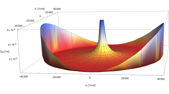
Figure 1: The spectral composition of the total photon production rate $S_{\gamma}(\mathbf{k})+S_{\mathrm{eh}}(\mathbf{k})$ in the long-wave region: the central $1/k$ peak corresponds to the annihilation channel, the peripheral distribution represents the momentum redistribution mechanism.

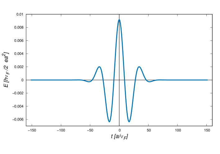
Figure 2: Dependence of field strength on time in the model of the short laser pulse (70). We used the natural graphene units for time $[a/v_{F}]$ and field strength $[\hbar v_{F}/ea^{2}]$ ($a$ is the graphene lattice constant).

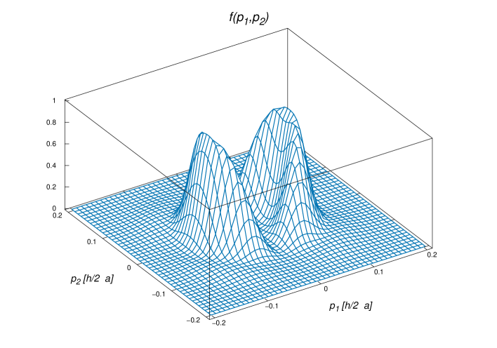
Figure 3: Distribution function $f(\mathbf{k},t\rightarrow\infty)$ after the end of the pulse calculated on the basis of KEs (27). The values of the momentum components are given in units of $[\hbar/a$].

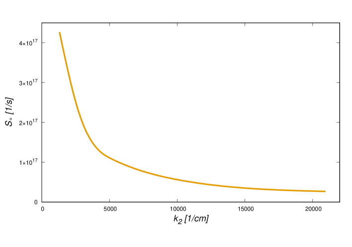
Figure 4: $1/k$ - structure of the CI (68) of the annihilation channel obtained as the result of direct numerical calculations $(k_{1}=0,\ t=100\ a/V)$

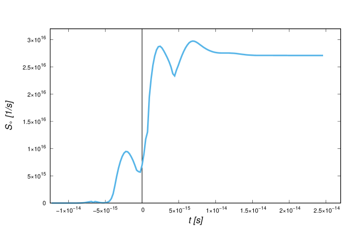
Figure 5: Time dependence of the collision integral $S_{\gamma}(\mathbf{k},t)$

$1/k$-dependence in the region of the central peak is reproduced also on the qualitative level by virtue of numerical calculations directly of CI (68) in the annihilation channel.

Specific of the computer calculations forces one to use the field model of a short laser impulse (71) (see Fig.2 for the case of linear polarization, $E_{0}=10^{6}\ {\mathrm{V}/cm},\ \omega=2\pi\times 10^{14}\ \mathrm{Hz},\ \sigma=3$). The distribution function of the eh-subsystem calculated on the basis of basic KE (27) is depicted for the point of time $t=0$ on the Fig.3. The valley $p_{1}=0$ between two symmetrical fragments of the distribution function is a consequence of the structure of amplitude (10) ($E_{\mathrm{ext}}^{1}(t)=0$ by virtue of the chosen polarization of the external field). At last, Fig.4 shows $1/k$ dependence in projection on the axis of $k_{2}$ calculated on the basis of CI (68) of the annihilation channel.

(6) As it was showed in Sect.5, the considered above CI in the model of periodical field (72) do not contain time independent components. This fact can be explained by the absence of a definite asymptotic limit of field model (72) at $t\rightarrow\infty$ Blaschke (2013). In the general case CI can have non-zero asymptotic at $t\rightarrow\infty$ if the back reaction of the system is not taken into account. Fig.5 demonstrates such situation in the model of a short laser pulse (70). We believe that a special consideration of such behavior is would be quite important.

6 Conclusion

In the present work we have considered some physical processes which are possible in the graphene under action of a strong time dependent electric field. To this end nonperturbative methods (see Gitman (1977); Fradkin (1981, 1991) and relevant Refs. given in the text of the article) of strong field QED with unstable vacuum (in particular, the Dirac model of the graphene) were used in combination with kinetic description of radiation from the electron-positron plasma created from the vacuum under an action of a strong time dependent electric field developed in Refs. Smolyansky (2020, 2020); Blaschke (2011); Smolyansky (2019); Otto (2017). We would like to emphasize the significant development of KE formalism and the study of the structure of these equation presented in the work. This formalism includes a nonperturbative basis oriented on the description of excitations of the eh-plasma in the graphene under the action of strong electric fields and a perturbative part described interaction with the quantized electromagnetic field. Main concrete results obtained in the work on the base of such generalized theory are presented in Subsect. 5.3. We stress that some of the predicted properties of the model under consideration may be verified experimentally. First, is the issue of the possible presence of even harmonics of the external field in the quantum radiation spectrum. Another important property that can be tested is the characteristic spectral composition anisotropy of the quantum radiation and its direction in the graphene plane (emission in the external space of the electromagnetic waves of the plasma oscillations is oriented perpendicular to the graphene plane). Some other predictions are related to the long wave features of this radiation. In this respect, we note that the developed approach can be extended to a wider range of parameters of the external field including into the consideration arbitrary polarizations. It is also important to consider in a similar manner such processes as photoproduction of the eh - plasma under the action of quantum electromagnetic field, cascade processes, the Breit-Wheeler process (e.g., Titov (2016)) and so on. We recall that a radiation of quasiclassical plasma waves in the graphene obtained in the frame work of the nonperturbative KE approach had got sufficiently reliable experimental testing (e.g., Smolyansky (2020) and having there references).

In the conclusion, it should be noted that the new extended formulation of KE approach contains some model assumptions. Further calculations in the frame work of the formulation may check validity of these assumptions. Such checking would be important for applications of strong field QED in $3+1$ dimensions, where the situation is more complicated.

This research was funded by Russian Science Foundation (Grant no. 19-12-00042)

References

- Klein (1929) Klein, O. Die Reflexion von Elektronen an einem Potentialsprung nach der relativistischen Dynamik von Dirac. Z. Physik 1929, 53, 157–165, doi:10.1007/BF01339716.
- Klein (1927) Klein, O. Elektrodynamik und Wellenmechanik vom Standpunkt des Korrespondenzprinzips. Z. Physik 1927, 41, 407–442, doi:10.1007/BF01400205.
- Sauter (1931) Sauter, F. Über das Verhalten eines Elektrons im homogenen elektrischen Feld nach der relativistischen Theorie Diracs. Z. Physik 1931, 69, 742–764, doi:10.1007/BF01339461.
- Sauter (1931) Sauter, F. Zum " Kleinschen Paradoxon" . Z. Physik 1932, 73, 547–552, doi:10.1007/BF01349862.
- Schwinger (1951) Schwinger, J. On Gauge Invariance and Vacuum Polarization. Phys. Rev. 1951, 82, 664–679, doi:10.1103/PhysRev.82.664.
- Nikishov (1970) Nikishov, A.I. Pair Production by a Constant Electric Field. Sov. Phys. JETP 1970, 30, 660–663. [Zh. Eksp. Teor. Fiz. 1969, 57, 1210].
- Nikishov (1970) Nikishov, A.I. Barrier scattering in field theory removal of klein paradox. Nucl. Phys. B 1970, 21, 346–358, doi:10.1016/0550-3213(70)90527-4.
- Nikishov (1985) Nikishov, A.I. Problems of intense external-field intensity in quantum electrodynamics. J Russ Laser Res 1985, 6, 619–717, doi:10.1007/BF01120143.
- Narozhnyi (1970) Narozhnyi, N.B.; Nikishov, A.I. The Simplist processes in the pair creating electric field. Sov. J. Nucl. Phys. 1970 11, 596. [Yad.Fiz. 1970, 11, 1072].
- Narozhnyi (1974) Narozhnyi, N.B.; Nikishov, A.I. Pair production by a periodic electric field. Sov. Phys. JETP 1974, 38, 427. [Zh. Eksp. Teor. Fiz. 1974, 65, 862].
- Ruffini (2010) Ruffini, R.; Vereshchagin, G.; Xue, S. Electron–positron pairs in physics and astrophysics: From heavy nuclei to black holes. Phys. Rep. 2010, 487, 1, doi:10.1016/j.physrep.2009.10.004.
- Gelis (2016) Gelis, F.; Tanji, N. Schwinger mechanism revisited. Prog. Part. Nucl. Phys. 2016, 87, 1, doi:10.1016/j.ppnp.2015.11.001.
- Gitman (1977) Gitman, D.M. Processes of arbitrary order in quantum electrodynamics with a pair-creating external field. J. Phys. A 1977, 10, 2007, doi:10.1088/0305-4470/10/11/026.
- Fradkin (1981) Fradkin, E.S.; Gitman, D.M. Furry Picture for Quantum Electrodynamics with Pair-Creating External Field. Fortschr. Phys. 1981, 29, 381–412, doi:10.1002/prop.19810290902.
- Fradkin (1991) Fradkin, E.S.; Gitman, D.M.; Shvartsman, S.M. Quantum Electrodynamics with Unstable Vacuum; Springer-Verlag: Berlin, Germany, 1991, ISBN 978-3-642-84260-3.
- Hansen (1981) Hansen, A.; Ravndal, F. Klein’s Paradox and Its Resolution. Phys. Scripta 1981 23, 1036, doi:10.1088/0031-8949/23/6/002.
- Gavrilov (2016) Gavrilov, S.P.; Gitman, D.M. Quantization of charged fields in the presence of critical potential steps. Phys. Rev. D 2016, 93, 045002, doi:10.1103/PhysRevD.93.045002.
- Bagrov (1975) Bagrov, V.G.; Gitman D.M.; Shvartsman, S.M. Concerning the production of electron-positron pairs from vacuum. Sov. Phys. JETP 1975, 41, 191–194. [Zh. Eksp. Teor. Fiz. 1975, 68, 392–399].
- Gavrilov (1996) Gavrilov S.P.; Gitman, D.M. Vacuum Instability in External Fields. Phys. Rev. D 1996, 53, 7162, doi:10.1103/PhysRevD.53.7162.
- Mostepanenko (1974) Mostepanenko, V.M.; Frolov, V.M. Production of particles from vacuum by a uniform electric-field with periodic time-dependence. Sov. J. Nucl. Phys. 1974, 19, 451–456,
- Adorno (2015) Adorno T.C.; Gavrilov S.P.; Gitman, D.M. Particle creation from the vacuum by an exponentially decreasing electric field. Phys. Scripta 2015, 90, 074005, doi:10.1088/0031-8949/90/7/074005.
- Adorno (2016) Adorno, T.C.; Gavrilov, S.P.; Gitman, D.M. Particle creation by peak electric field. Eur. Phys. J. C 2016, 76, 447, doi:10.1140/epjc/s10052-016-4289-0.
- Adorno (2017) Adorno, T.C.; Ferreira, R.; Gavrilov, S.P.; Gitman, D.M. Peculiarities of Pair Creation by a Peak Electric Field. Russ. Phys. J. 2017, 60, 417, doi:10.1007/s11182-017-1090-y.
- Adorno (2017) Adorno, T.C.; Gavrilov, S.P.; Gitman, D.M. Exactly solvable cases in QED with -electric potential steps. Int. J. Mod. Phys. A 2017, 32, 1750105, doi:10.1142/S0217751X17501056.
- Adorno (2018) Adorno, T.C.; Ferreira, R.; Gavrilov S.P.; Gitman, D.M. Role of switching-on and -off effects in the vacuum instability. Int. J. Mod. Phys. A 2018, 33, 1850060, doi:10.1142/S0217751X18500604.
- Adorno (2018) Adorno, T.C.; Gavrilov S.P.; Gitman, D.M. Violation of vacuum stability by inverse square electric fields. Eur. Phys. J. C 2018, 78, 1021, doi:10.1140/epjc/s10052-018-6499-0.
- Gavrilov (2016) Gavrilov, S.P.; Gitman, D.M. Scattering and pair creation by a constant electric field between two capacitor plates. Phys. Rev. D 2016, 93, 045033, doi:10.1103/PhysRevD.93.045033.
- Gavrilov (2017) Gavrilov, S.P.; Gitman, D.M.; Shishmarev, A.A. Particle scattering and vacuum instability by exponential steps. Phys. Rev. D 2017, 96, 096020, doi:10.1103/PhysRevD.96.096020.
- Adorno (2020) Adorno, T.C.; Gavrilov, S.P.; Gitman, D.M. Vacuum instability in a constant inhomogeneous electric field: a new example of exact nonperturbative calculations. Eur. Phys. J. C 2020, 80, 88, doi:10.1140/epjc/s10052-020-7646-y.
- Dunne (2009) Dunne, G.V. New strong-field QED effects at extreme light infrastructure. Eur. Phys. J. D 2009, 55, 327–340, doi:10.1140/epjd/e2009-00022-0.
- Castro Neto (2009) Castro Neto, A.H.; Guinea, F.; Peres, N.M.R.; Novoselov, K.S.; Geim, A.K. The electronic properties of graphene. Rev. Mod. Phys. 2009, 81, 109, doi:10.1103/RevModPhys.81.109.
- Peres (2010) Peres, N.M.R. Colloquium: The transport properties of graphene: An introduction. Rev. Mod. Phys. 2010, 82, 2673, doi:10.1103/RevModPhys.82.2673.
- Vozmediano (2010) Vozmediano, M.A.H.; Katsnelson, M.I.; Guinea, F. Gauge fields in graphene. Phys. Rep. 2010, 496, 109–148, doi:10.1016/j.physrep.2010.07.003.
- Das Sarma (2011) Das Sarma, D.; Adam, S.; Hwang, E.H.; Rossi, E. Electronic transport in two-dimensional graphen. Rev. Mod. Phys. 2011, 83, 407, doi:10.1103/RevModPhys.83.407.
- Semenoff (1984) Semenoff, G.W. Condensed-Matter Simulation of a Three-Dimensional Anomaly. Phys. Rev. Lett. 1984, 53, 2449, doi:10.1103/PhysRevLett.53.2449.
- Allor (2008) Allor, D.; Cohen, T.D.; McGady, D.A. The Schwinger mechanism and graphene. Phys. Rev. D 2008, 78, 096009, doi:10.1103/PhysRevD.78.096009.
- Dóra (2010) Dóra, B.; Moessner, R. Nonlinear electric transport in graphene: Quantum quench dynamics and the Schwinger mechanism. Phys. Rev. B 2010, 81, 165431, doi:10.1103/PhysRevB.81.165431.
- Lewkowicz (2009) Lewkowicz, M.; Rosenstein, B. Dynamics of Particle-Hole Pair Creation in Graphene. Phys. Rev. Lett. 2009, 102, 106802, doi:10.1103/PhysRevLett.102.106802.
- Rosenstein (2010) Rosenstein, B.; Lewkowicz, M.; Kao, H.C.; Korniyenko, Y. Ballistic transport in graphene beyond linear response. Phys. Rev. B 2010, 81, 041416(R), doi:10.1103/PhysRevB.81.041416.
- Kao (2010) Kao, H.C.; Lewkowicz M.; Rosenstein, B. Ballistic transport, chiral anomaly, and emergence of the neutral electron-hole plasma in graphene. Phys. Rev. B 2010, 82, 035406, doi:10.1103/PhysRevB.82.035406.
- Lewkowicz (2011) Lewkowicz, M.; Kao, H.C.; Rosenstein, B. Signature of the Schwinger pair creation rate via radiation generated in graphene by a strong electric current. Phys. Rev. B 2011, 84, 035414, doi:10.1103/PhysRevB.84.035414.
- Vandecasteele (2010) Vandecasteele, N.; Barreiro, A.; Lazzeri, M.; Bachtold, A.; Mauri, F. Current-voltage characteristics of graphene devices: Interplay between Zener-Klein tunneling and defects. Phys. Rev. B 2010, 82, 045416, doi:10.1103/PhysRevB.82.045416.
- Gavrilov (2012) Gavrilov, S.P.; Gitman, D.M.; Yokomizo, N. Dirac fermions in strong electric field and quantum transport in graphene. Phys. Rev. D 2012, 86, 125022, doi:10.1103/PhysRevD.86.125022.
- Gavrilov (2016) Gavrilov, S.P. and Gitman, D.M. Radiative Processes in Graphene and Similar Nanostructures at Strong Electric Fields. Izvestia Vysshih Uchebnih Zavedeniy, Fiz. 2016, 59 , No. 11, 123-126 [Translation: Rus. Phys. J. 2017, 59, No. 11, 1870-1874. (In English)] doi: 10.1007/s11182-017-0989-7
- Popov (1973) Popov, V.S.; Marinov, M.S. - Pair production in variable electric field. Sov. J. Nucl. Phys. 1973, 16, 449. [Yad. Fiz. 1972, 16, 809–822].
- Grib (1934) Grib A.A.; Mamaev, S.G.; Mostepanenko, V.M. Vacuum Quantum Effects in Strong Fields; Friedmann Laboratory Publishing: St.Petersburg, Russia, 1994.
- Bialynicky-Birula (1991) Bialynicky-Birula, I.; Gornicki, P.; Rafelski, J. Phase space structure of the Dirac vacuum. Phys. Rev. D 1991, 44, 1825, doi:10.1103/PhysRevD.44.1825.
- Schmidt (1998) Schmidt, S.M.; Blaschke, D.; Röpke, G.; Smolyansky, S.A.; Prozorkevich, A.V.; Toneev, V.D. A Quantum kinetic equation for particle production in the Schwinger mechanism. Int. J. Mod. Phys. E 1998, 7, 709–718, doi:10.1142/S0218301398000403.
- Kluger (1998) Kluger, Y.; Mottola, E.; Eisenberg, J. Quantum Vlasov equation and its Markov limit. Phys. Rev. D 1998, 58, 125015, doi:10.1103/PhysRevD.58.125015.
- Mamaev (1979) Mamaev, S.G.; Trunov, N.N. Vacuum polarization and particle production in a non-stationary homogeneous electromagnetic field. Sov. J. Nucl. Phys. 1979, 30, 677. [Yad. Fiz. 1979, 30, 1301–1311].
- Dumlu (2009) Dumlu, C.K. Quantum kinetic approach and the scattering approach to vacuum pair production. Phys. Rev. D 2009, 79, 065027, doi:10.1103/PhysRevD.79.065027.
- Fedotov (2011) Fedotov, A.M.; Gelfer, E.G.; Korolev, K.Yu.; Smolyansky, S.A. Kinetic equation approach to pair production by a time-dependent electric field. Phys. Rev. D 2011, 83, 025011, doi:10.1103/PhysRevD.83.025011.
- Blaschke (2017) Blaschke, D.B.; Smolyansky, S.A.; Panferov, A.D.; Juchnowski, L. Particle Production in Strong Time-dependent Fields. arXiv 2017, arXiv:1704.04147.
- Smolyansky (2019) Smolyansky, S.A.; Panferov, A.; Blaschke, D.; Gevorgayn, N. Nonperturbative Kinetic Description of Electron-Hole Excitations in Graphene in a Time Dependent Electric Field of Arbitrary Polarization. Particles 2019, 2, 208–230, doi:10.3390/particles2020015.
- Panferov (2017) Panferov, A.D.; Churochkin, D.V.; Fedotov, A.M.; Smolyansky, S.A.; Blaschke, D.B.; Gevorgyan, N.T. Nonperturbative kinetic description of e-h excitations in graphene due to a strong, time-dependent electric field. In Proceedings of the Ginzburg Centennial Conference on Physics, May 29 - June 3, 2017, Moscow. Available online: http://gc2.lpi.ru/proceedings/panferov.pdf (accessed on 16 March 2020).
- Smolyansky (2019) Smolyansky, S.A.; Blaschke, D.B.; Dmitriev, V.V.; Panferov, A.D.; Gevorgyan, N.T. Back reaction in graphene excited by a strong laser field. Presented at the Helmholtz International Summer School, 22 July - 2 August, 2019, Dubna. Available online: https://indico.jinr.ru/event/797/material/slides/9.pdf (accessed on 16 March 2020).
- Blaschke (2011) Blaschke, D.B.; Dmitriev, V.V.; Röpke, G.; Smolyansky, S.A. BBGKY kinetic approach for an plasma created from the vacuum in a strong laser-generated electric field: The one-photon annihilation channel. Phys. Rev. D 2011, 84, 085028, doi:10.1103/PhysRevD.84.085028.
- Smolyansky (2019) Smolyansky, S.A.; Panferov, A.D.; Pirogov, S.O.; Fedotov, A.M. Self-consistent kinetic equations for -plasma generated from vacuum by strong electric field. arXiv 2019, arXiv:1901.02305.
- Bloch (1999) Bloch, J.C.R.; Mizerny, V.A.; Prozorkevich, A.V.; Roberts, C.D.; Schmidt, S.M.; Smolyansky, S.A.; Vinnik, D.V. Pair creation: Back reactions and damping. Phys. Rev. D 1999, 60, 116011, doi:10.1103/PhysRevD.60.116011.
- Abbott (1985) Abbott, T.A.; Griffiths, D.J. Acceleration without radiation. Am. J. Phys. 1985, 53, 1203–1211, doi:10.1119/1.14084.
- Baudisch (2018) Baudisch, M.; Marini, A.; Cox, J.D.; Zhu, T.; Silva, F.; Teichmann, S.; Massicotte, M.; Koppens, F.; Levitov, L.S.; García de Abajo, F.J.; et al. Ultrafast nonlinear optical response of Dirac fermions in graphene. Nat. Commun. 2018, 9, 1–6, doi:10.1038/s41467-018-03413-7.
- Bowlan (2014) Bowlan, P.; Martinez-Moreno, E.; Reimann, K.; Elsaesser, T.; Woerner, M. Ultrafast terahertz response of multilayer graphene in the nonperturbative regime. Phys. Rev. B. 2014, 89, 041408, doi:10.1103/PhysRevB.89.041408.
- Smolyansky (2020) Smolyansky, S.A.; Panferov, A.D.; Blaschke, D.B.; Gevorgyan, N.T. Kinetic Equation Approach to Graphene in Strong External Fields. Particles 2020, 3(2), 456–476, doi:10.3390/particles3020032.
- Ishikava (2010) Ishikava, K.L. Nonlinear optical response of graphene in time domain. Phys. Rev. B 2010, 82, 201402(R), doi:10.1103/PhysRevB.82.201402.
- Ishikava (2013) Ishikava, K.L. Electronic response of graphene to an ultrashort intense terahertz radiation pulse. New J.of Phys. 2013, 15, 055021, doi:10.1088/1367-2630/15/5/055021.
- Smolyansky (2020) Smolyansky, S.A.; Fedotov, A.M.; Dmitriev, V.V. Kinetics of the vacuum plasma in a strong electric field and problem of radiation. Mod. Phys. Lett. A. 2020, 35, 2040028, doi:10.1142/S0217732320400283.
- Otto (2017) Otto, A.; Kämpfer, B. Afterglow of the dynamical Schwinger process: Soft photons amass. Phys. Rev. D 2017, 95, 125007, doi:10.1103/PhysRevD.95.125007.
- deGroot (1980) de Groot, S.R.; van Leeuwen, W.A.; van Weert, Ch.Gvistic. Kinetic theory: Principles and application; North-Hollan Comp.; Amsterdam, New York, Oxford, 1980.
- Kadanoff (1962) Kadanoff, L.P.; Baym, G. Quantum Statistical Mechanics; Pines, D. Eds.; W.A. Benjamin, Inc: New York, USA, 1962, ISBN 978-0367320102.
- Zubarev (1966) Zubarev, D.; Morozov, V.; Röpke, G. Statistical Mechanics of Nonequilibrium Processes; Akademie Verlag: Berlin, Germany, 1996; Volume 1, ISBN 3-05-501708-0.
- Novoselov (2005) Novoselov, K.S.; Geim, A.K.; Morozov, S.V.; Jiang, D.; Katsnelson, M.I.; Grigorieva, I.V.; Dubonos, S.V.; Firsov, A.A. Two-dimensional gas of massless Dirac fermions in graphene. Nature 2005, 438, 197–200, doi:10.1038/nature04233.
- Geim (2007) Geim, A.K.; Novoselov, K.S. The rise of graphene. Nat. Mater. 2007, 6, 183–191, doi:10.1038/nmat1849.
- Gusynin (2007) Gusynin, V.P.; Sharapov, S.G.; Carbotte, J.P. AC Conductivity of Graphene from Tight-Binding Model to 2+1 Dimensional Quantum Electrodynamics. Int. J. of Mod. Phys. B 2007, 21, 4611, doi:10.1142/S0217979207038022.
- Dabrowski (2014) Dabrowski, R.; Dunne,G.V. Super-adiabatic Particle Number in Schwinger and de Sitter Particle Production. Phys. Rev. D 2014, 90, 025021, doi:10.1103/PhysRevD.90.025021.
- Klimchitskaya (2013) Klimchitskaya, G.L.; Mostepanenko, V.M. Creation of quasiparticles in graphene by a time-dependent electric field. Phys. Rev. D 2013, 87, 125011, doi:10.1103/PhysRevD.87.125011.
- Blaschke (2009) Blaschke, D.B.; Prozorkevich, A.V.; Röpke, G.; Roberts, C.D.; Schmidt, S.M.; Shkirmanov, D.S.; Smolyansky, S.A. Dynamical Schwinger effect and high-intensity lasers. realising nonperturbative QED. Eur. Phys. J. D 2009, 55, 341, doi:10.1140/epjd/e2009-00156-y.
- Hebenstreit (2009) Hebenstreit, F.; Alkofer, R.; Dunne, G.V.; Gies, H. Momentum Signatures for Schwinger Pair Production in Short Laser Pulses with a Subcycle Structure. Phys. Rev. Lett. 2009, 102, 150404, doi:10.1103/PhysRevLett.102.150404.
- Amirov (1974) Amirov, R.Kh.; Smolyanskii S.A.; Shechter, L.Sh. On the theory of quantum kinetic processes in strong alternating fields. Theor Math Phys 1974, 21, 1116–1124, doi:10.1007/BF01035559.
- Seminozhenko (1982) Seminozhenko, V.P. Kinetics of interacting quasiparticles in strong external fields. Phys. Rep. 1982, 91, 105, doi:10.1016/0370-1573(82)90049-7.
- Smolyansky (2020) Smolyansky, S.A.; Fedotov, A.M.; Dmitriev, V.V. BBGKY Method in Strong Field QED. PEPAN 2020, 51, 595–598, doi:10.1134/S106377962004067X.
- Blaschke (2013) Blaschke, D.B.; Kämpfer B., Schmidt, S.M.; Panferov, A.D.; Prozorkevich, A.V.; Smolyansky, S.A. Properties of the electron-positron plasma created from a vacuum in a strong laser field: Quasiparticle excitations. Phys. Rev. D 2013, 88, 045017, doi:10.1103/PhysRevD.88.045017.
- Titov (2016) Titov, A.I.; Kämpfer, B.; Hosaka, A.; Takabe, H. Quantum Processes in Short and Intensive Electromagnetic Fields. PEPAN 2016, 47, 835–899.