Soliton gas in bidirectional dispersive hydrodynamics
Abstract
The theory of soliton gas had been previously developed for unidirectional integrable dispersive hydrodynamics in which the soliton gas properties are determined by the overtaking elastic pairwise interactions between solitons. In this paper, we extend this theory to soliton gases in bidirectional integrable Eulerian systems where both head-on and overtaking collisions of solitons take place. We distinguish between two qualitatively different types of bidirectional soliton gases: isotropic gases, in which the position shifts accompanying the head-on and overtaking soliton collisions have the same sign, and anisotropic gases, in which the position shifts for head-on and overtaking collisions have opposite signs. We construct kinetic equations for both types of bidirectional soliton gases and solve the respective shock-tube problems for the collision of two “monochromatic” soliton beams consisting of solitons of approximately the same amplitude and velocity. The corresponding weak solutions of the kinetic equations consisting of differing uniform states separated by contact discontinuities for the mean flow are constructed. Concrete examples of bidirectional Eulerian soliton gases for the defocusing nonlinear Schrödinger (NLS) equation and the resonant NLS equation are considered. The kinetic equation of the resonant NLS soliton gas is shown to be equivalent to that of the shallow-water bidirectional soliton gas described by the Kaup-Boussinesq equations. The analytical results for shock-tube Riemann problems for bidirectional soliton gases are shown to be in excellent agreement with direct numerical simulations.
I Introduction
Dispersive hydrodynamics modeled by hyperbolic conservation laws regularized by conservative, dispersive corrections describe various nonlinear wave structures that include solitary waves (solitons), dispersive shock waves (DSWs), rarefaction waves and their interactions biondini_dispersive_2016 . A particular feature of dispersive hydrodynamics is the intrinsic scale separation, often providing a qualitatively new perspective on some classical mathematical and fluid dynamical settings (such as Riemann problems or flows past topography), but also revealing novel phenomena such as hydrodynamic soliton tunneling maiden_solitonic_2018 ; sprenger_hydrodynamic_2018 and expansion shocks el_expansion_2016 .
On a small-scale, microscopic, level dispersive hydrodynamics typically involve coherent nonlinear wave structures such as solitons and rapidly oscillating periodic waves, while the large-scale, macroscopic coherent features are represented by slow modulations of these periodic waves or soliton trains. The prominent example of a dispersive hydrodynamic structure exhibiting such two-scale coherence and persisting in integrable and non-integrable systems is DSW, the dispersive analog of a classical, viscous shock wave el_dispersive_2016 .
There is another class of problems in dispersive hydrodynamics, which involve the wave structures exhibiting coherence at a microscopic scale, while being macroscopically incoherent, in the sense that the values of the wave field at two points separated by a distance much larger than the intrinsic dispersive length of the system (the soliton width), are not dynamically related. These structures can be broadly viewed as dispersive-hydrodynamic analogs of turbulence, and the qualitative and quantitative properties of such a conservative turbulence strongly depend on the integrability properties of the underlying microscopic dynamics. In zakharov_turbulence_2009 V.E. Zakharov introduced the notion of “integrable turbulence” for random nonlinear wave fields governed by integrable equations such as the Korteweg-de Vries (KdV) or Nonlinear Schrödinger (NLS) equations. The source of randomness in integrable turbulence is typically related to some sort of stochastic initial or boundary conditions although one can envisage dynamical mechanisms of the effective randomization of the wave field gurevich_development_1999 ; el_dam_2016 . The theoretical perspective of integrable turbulence has turned out to be very fruitful, providing new insights into some long-standing problems of nonlinear physics related e.g. to modulational instability and the formation of rogue waves Walczak:15 ; Randoux:16b ; gelash_strongly_2018 . Indeed, integrable turbulence proved a promising theoretical framework for the interpretation of experimental and observational data in fiber optics and fluid dynamics costa_soliton_2014 .
Solitons, viewed as stable “wave-particles” of macroscopic dispersive-hydrodynamic structures, can form large disordered, statistical ensembles, strikingly different from the macroscopically coherent DSWs, and calling for the analogy with gases of classical or quantum particles. Such statistical soliton ensembles, or “soliton gases”, can be naturally generated from both non-vanishing deterministic (e.g. periodic or quasiperiodic) and random initial conditions due to the processes of soliton fissioning trillo_experimental_2016 ; trillo_observation_2016 or modulation instability gelash_bound_2019 . The ubiquity of solitons in applications and the integrable nature of the underlying wave dynamics makes soliton gases a particularly attractive object for modeling the complex nonlinear wave phenomena occurring in the ocean and in high-intensity incoherent light propagation through optical materials, see el_spectral_2020 and references therein. The random nonlinear wave field in a soliton gas represents a particular case of integrable turbulence zakharov_turbulence_2009 .
Within the inverse scattering transform (IST) formalism each soliton is characterized by a discrete eigenvalue of the spectrum of the linear operator associated with the integrable nonlinear evolution equation. There are two basic aspects of the microscopic, soliton dynamics that determine the macroscopic, statistical properties of integrable soliton gases/turbulence: (i) isospectrality of integrable evolution resulting in the preservation of soliton eigenvalues; (ii) pairwise elastic collisions accompanied by phase/position shifts expressed in terms of the respective spectral parameters of the interacting solitons.
The macroscopic properties of a soliton gas are determined by the spectral characteristics called the density of states (DOS) , defined such that the number of solitons found at the moment of time in the element of the phase space is (assuming , the generalization to complex spectrum being straightforward el_kinetic_2005 ). DOS represents the definitive statistical characteristics of soliton gas distinguishing it from an arbitrary random collection of solitons. The first controlled generation of soliton gas characterized by a measurable DOS has been recently reported in suret_nonlinear_2020 .
For uniform, statistically homogeneous soliton gases the DOS depends on the spectral parameter only. For spatially nonhomogeneous soliton gases one has , and the isospectrality of integrable evolution implies the conservation equation
| (1) |
where the transport velocity (the mean velocity of a “tracer” soliton in a gas) is found from the integral equation of state el_kinetic_2005
| (2) |
Here is the velocity of an isolated single soliton with the spectral parameter , and the integral term describes its modification due to collisions with other, “-solitons” in a gas, each collision being accompanied by the position shift , often called the phase shift. The integration in (I) is performed over the spectral support of the DOS . If one assumes that (i) ; and (ii) the modulus sign in (I) can be removed by introducing so that one arrives at the conventional form of the equation of state as in el_kinetic_2005 ; el_kinetic_2011 , involving rather than as the integral kernel. E.g. for the KdV solitons one has , and (see e.g. ablowitz_note_1982 ).
The transport equation (1) for the DOS complemented by the integral equation of state (I) comprise the kinetic equation for soliton gas. Kinetic equation of the type (1),(I) was first introduced in zakharov_kinetic_1971 for the case of rarefied, or dilute, gas of KdV solitons, when the interaction term in the equation state (I) represents a small correction and the soliton velocity in a gas is found from the expression , which is an approximate solution of the equation of state (I) for the KdV soliton gas. The full kinetic equation (1),(I) for a dense soliton gas was derived and analyzed in the context of the KdV equation in el_thermodynamic_2003 ; el_critical_2016 and the focusing NLS equation in el_kinetic_2005 ; el_spectral_2020 (in the latter case ). A general mathematical analysis of the kinetic equation (1),(I) has been undertaken in el_kinetic_2011 , which showed that it possesses an infinite series of integrable linearly degenerate hyperbolic reductions. Very recently the kinetic equation (1),(I) has attracted much attention in the context of generalized hydrodynamics, a statistical theory of quantum many-body integrable systems, see doyon_soliton_2018 ; doyon_geometric_2018 ; vu_equations_2019 and references therein.
In the context of dispersive hydrodynamics the kinetic equation (1),(I) describes “unidirectional” soliton gases supported by scalar integrable equations of the form
| (3) |
where is the nonlinear hyperbolic flux and is a differential (generally integro-differential) operator, possibly nonlinear, that gives rise to a real-valued linear dispersion relation. The spectral single-soliton solutions to Eq. (3) are characterized by the soliton velocity and the phase shift kernel characterizing the “overtaking” two-soliton interactions. However, the scalar integrable dispersive hydrodynamics of the form (3), such as the KdV, modified KdV, Camassa-Holm or Benjamin-Ono equations typically arise as small-amplitude, “unidirectional” approximations of more general Eulerian bidirectional systems (see whitham_linear_1999 )
| (4) |
where are conservative, dispersive operators, is the monotonically increasing pressure law, and , are interpreted as a mass density and fluid velocity, respectively. This class of equations generalizes the shallow water and isentropic gas dynamics equations while encompassing many of the integrable dispersive hydrodynamic models such as the Kaup-Boussinesq (KB) system kaup_higher_1975 , the hydrodynamic form of the defocusing NLS equation kamchatnov_nonlinear_2000 or the Calogero-Sutherland system describing the dispersive hydrodynamics of quantum many-body systems abanov_integrable_2009 . Due to the bidirectional nature, the Eulerian dispersive hydrodynamics (4) supports solitons that experience both overtaking and head-on elastic collisions which are generally characterized by two different phase shift kernels . Indeed, the rarefied bidirectional shallow-water soliton gas realized in the water tank experiments redor_experimental_2019 ; redor_analysis_2020 was modeled by the KB system kaup_higher_1975 , which exhibits qualitatively different properties for head-on and overtaking position shifts in the pairwise soliton collisions li_bidirectional_2003 so that the overtaking interactions can be characterized as “strong” and the head-on interactions as “weak”. We shall term such collisions and the associated soliton gases as “anisotropic”. On the other hand, some bidirectional dispersive hydrodynamic systems support soliton solutions that exhibit “isotropic” collisions characterized by the same phase shift kernel for the head-on and overtaking interactions (e.g. the defocusing NLS equation zakharov_interaction_1973 ).
Despite the significant recent advances of the kinetic theory of unidirectional soliton gases, a consistent general extension of this theory to the physically important bidirectional case has not been available so far, and this paper is devoted to the development of such an extension. The paper is organized as follows. In Section II we present the general construction of the kinetic equation for bidirectional soliton gas and realize it for the cases of the defocusing nonlinear Schrödinger (DNLS) equation and its “stable” negative dispersion counterpart, the so-called resonant NLS (RNLS) equation, having applications in magneto-hydrodynamics of cold collisionless plasma lee_resonant_2007 , and reducible to the KB system for shallow-water waves by a simple change of variables. It turns out that, due to the pairwise collisions of dark DNLS solitons being isotropic, the bidirectional kinetic equation for the dark (grey) solitons of the DNLS equation reduces to the unidirectional kinetic equation of the form (1),(I). Contrastingly, the soliton collisions of anti-dark RNLS solitons are anisotropic, and the kinetic equation for this case represents a pair of the kinetic equations of the type (1),(I) with some nonlinear coupling through the equation of state. In Section III we derive expressions for the mean field in both soliton gases in terms of the spectral DOS. To demonstrate the efficacy of the developed theory we consider in Section IV the “shock-tube” Riemann problem describing the collision of “monochromatic” soliton beams for both types of bidirectional gases. The collisions are described by weak solutions to the bidirectional kinetic equations, consisting of a number differing constant states for the DOS, separated by contact discontinuities for the component densities, satisfying appropriate Rankine-Hugoniot conditions. The analytical results are shown to be in an excellent agreement with direct numerical simulations of the soliton gas shock-tube problem for DNLS and RNLS equations.
II Kinetic equation for bidirectional soliton gas
In this section we derive the kinetic equation for integrable Eulerian dispersive hydrodynamics (4) using the general physical construction proposed in el_kinetic_2005 for a uni-directional case. The construction uses an extension of the original Zakharov’s phase shift reasoning zakharov_kinetic_1971 , which, strictly speaking, is applicable only in a rarefied gas case. However, the resulting kinetic equation (1),(I) turns out to provide correct description for a dense gas, mathematically justified by the thermodynamic limit of the finite-gap Whitham modulation systems for the cases of the KdV el_thermodynamic_2003 and the focusing NLS el_spectral_2020 equations. Our results for bidirectional gas will be later supported by comparisons with direct numerical simulations of the relevant soliton gases, justifying the validity of the phenomenological derivation.
II.1 Isotropic and anisotropic bidirectional soliton gases
Suppose that the system (4) supports a family of bidirectional soliton solutions that bifurcate from the two branches of the linear wave spectrum of (4) so that in the long wavelength limit . We denote the corresponding soliton families and . Let these soliton solutions be parameterized by a real-valued spectral (IST) parameter so that for the “fast” branch and for the “slow” branch, where are simply-connected subsets of with one intersection point at most. Let the respective soliton velocities be . For convenience we assume that , and if and , . If we assume . The above assumptions are consistent with all concrete examples of integrable dispersive hydrodynamics we consider in this paper.
One can distinguish between two types of the pairwise collisions in a bidirectional soliton gas: the overtaking collisions between solitons belonging to the same spectral branch and characterized by the position shifts and respectively, and the “head-on” collisions between solitons of different branches, characterized by the position shifts and . Let , and and denote the position shifts of a -soliton due to its collision with a -soliton, with the first and the second signs in the subscript indicating the branch belonging of the -soliton and the -soliton respectively, e.g. is the position shift of a -soliton with in a collision with a -soliton with .
We call the bidirectional soliton gas “isotropic” if the position shifts for the overtaking and head-on collisions between - and - solitons satisfy the following sign conditions:
| (5) |
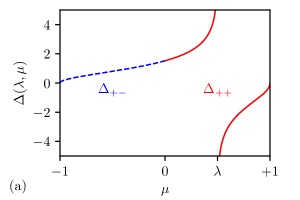
i.e. the -soliton experiences a shift of a certain sign, say shift forward (and the -soliton— the shift of an opposite sign) irrespectively of the type of the collision—overtaking or head-on. If conditions (5) are not satisfied, i.e. the sign of the phase shift depends on the type of the collision, we shall call the corresponding soliton gas “anisotropic”. The difference between isotropic and anisotropic collisions is illustrated in Fig. 1 using concrete examples.
II.2 Kinetic equation for bidirectional soliton gas: general construction
Following the construction for unidirectional soliton gas outlined in the introduction, we now consider bidirectional soliton gases for integrable Eulerian equations (4). We introduce two separate DOS’s and for the populations of solitons whose spectral parameters belong to the slow () and fast () branches of the spectral set respectively. The isospectrality of integrable evolution implies now two separate conservation laws:
| (6) |
where and are the transport velocities associated with the motion of slow solitons and fast solitons associated with and branches respectively. We derive the equations of state for using the direct phenomenological approach proposed el_kinetic_2005 : we identify as the velocity of a trial -soliton of the gas. Consider, for instance, a tracer -soliton from the slow branch, , and compute its displacement in a gas over the “mesoscopic” time interval , sufficiently large to incorporate a large number of collisions, but sufficiently small to ensure that the spatiotemporal field is stationary over and homogeneous on a typical spatial scale . Having this in mind, we drop the -dependence for convenience. Each overtaking collision with a soliton of the same branch shifts the -soliton by the distance . Thus the displacement of the -soliton over the time due to the overtaking collisions is given by where is the average number of collisions with encountered -solitons (cf. el_kinetic_2005 ). Additionally, each head-on collision with a fast soliton shifts the slow -soliton with by , and the resulting displacement after a time is . A similar consideration is applied to the fast soliton branch, , in the gas. Equating the total displacements of the slow and fast -solitons to and respectively, we obtain the equation of state of a bidirectional gas in the form of two coupled linear integral equations:
| (7) |
where for the first equation and for the second equation. If the spectral support is a simply connected set and the gas is isotropic, the distinction between the fast and slow branches becomes unnecessary and the kinetic equation (6),(7) for bidirectional soliton gas is naturally reduced to the unidirectional gas equation (1),(I) for a single DOS defined on the entire set . We will show in Sec. IV, using concrete examples, that the dynamics governed by the kinetic equations (1),(I) and (6),(7) is in a very good agreement with the results of direct numerical simulations of isotropic and anisotropic bidirectional soliton gases respectively.
II.3 Kinetic equation for bidirectional soliton gas: examples
As a representative (and physically relevant) example, we consider the integrable Eulerian dispersive hydrodynamics
| (8) |
For , system (8) is equivalent to the defocusing nonlinear Schrödinger (DNLS) equation:
| (9) |
The DNLS equation has a number of physical applications. In particular it describes propagation of light beams through optical fibers in the regime of normal dispersion, as well as nonlinear matter waves in quasi-1D repulsive Bose-Einstein condensates (BECs), see for instance yang_nonlinear_2010 . Pertinent to the present context, rarefied gas of dark solitons in quasi-1D BEC has been investigated in schmidt_non-thermal_2012 ; wang_transitions_2015 .
The DNLS equation has a family of dark (or grey) soliton solutions zakharov_interaction_1973
| (10) |
where for the slow solitons branch and for the fast solitons branch; note that solutions and have the same analytical expression.
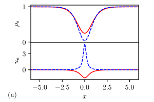
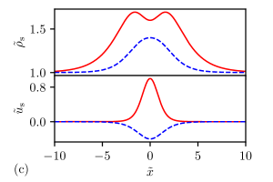
Without loss of generality we assumed in (10) the unit density background. Typical dark soliton solutions are displayed in Fig. 2. The position shifts in the DNLS overtaking and head-on soliton collisions are given by the same analytical expression , where
| (11) |
for all . One can verify that the soliton position shifts given by (11) satisfy the isotropy conditions (5). The variation of with respect to for a fixed is displayed in Fig. 1. One can see that the position shifts for the head-on and overtaking collisions lie on the same curve with being continuous at , the point of intersection of and . Due to the isotropic nature of the DNLS soliton interactions the coupled kinetic equation (6),(7) for the bidirectional DNLS gas reduces to the single kinetic equation (1) with the equation of state
| (12) |
where and with the assumption that ; the latter assumption is verified by comparison to numerics in Sec. IV.2. This reduction to the unidirectional case is similar to the kinetic equation derived in el_spectral_2020 for the bidirectional soliton and breather gases of the focusing NLS equation which also exhibits isotropic soliton/breather collisions, with the essential difference that the integration in the focusing NLS case occurs over a compact domain in a complex plane of the spectral parameter.
For the system (8) is equivalent to the so-called resonant NLS (RNLS) equation (see, e.g., lee_solitons_2007 )
| (13) |
This equation, in particular, describes long magneto-acoustic waves in a cold plasma propagating across the magnetic field gurevich_origin_1988 . The RNLS equation has a family of anti-dark soliton solutions given by lee_solitons_2007
| (14) |
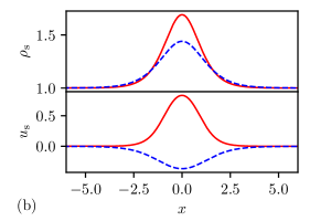
Solutions and have the same analytical expression. Typical anti-dark soliton solutions are displayed in Fig. 2.
In contrast with the DNLS system, the spectral set of the RNLS soliton is spanned by two disconnected subsets: for slow solitons and . Similar to the DNLS equation, the position shifts in head-on and overtaking collisions are given by the same analytical expression , where
| (15) |
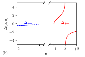
However, one can verify that, unlike in the DNLS case, the isotropy condition (5) is not satisfied. Indeed, it follows from (15) that , whereas , that is in a head-on collision between a -soliton and a -soliton with , the -soliton’s position is now shifted backward. The variation of for the RNLS equation shown in Fig. 1. One can see that it is qualitatively different from the variation of for the DNLS equation.
The kinetic equation for the anisotropic RNLS soliton gas has then the form of two continuity equations (6) complemented by the coupled equations of state
| (16) |
with the assumptions that and ; the latter assumption is verified by direct comparison with numerics in Sec. IV.2.
We note that the change of variables:
| (17) |
transforms the RNLS equation into the KB system kaup_higher_1975 :
| (18) |
describing bidirectional shallow water waves. The soliton solution of (18) is obtained by transforming (14) with the change of variables (17) (cf. Appendix A), and the phase of a -soliton after colliding with a -soliton is: . Thus the the RNLS and the KB soliton gas share the same anisotropic kinetic description. One can notice in Fig. 2 that the bimodal soliton of KB system transforms into a unimodal soliton of the RNLS equation with the change of variables (17).
In the numerical examples presented in the next section we will mostly focus on the anisotropic RNLS soliton gas for a direct comparison with the isotropic DNLS soliton gas.
III Ensemble averages of the wave field in bidirectional soliton gases
The DOS ( in the anisotropic case) represents a comprehensive spectral characteristics, that, in principle, determines all statistical parameters of the nonlinear random wave field in a soliton gas. The most obvious set of such statistical parameters are the ensemble averages of the conserved quantities. We note that for the KdV soliton gas the averages , were determined in terms of DOS in el_soliton_2001 ; el_critical_2016 using the machinery of finite-gap integration method. In this section we propose a simple heuristic approach that enables one to link the spectral DOS (or ) of a soliton gas with the ensemble averages of conserved quantities of the integrable system (4). As an illustration we consider the three first conserved densities of the Euler system (4): , and .
We first consider a homogeneous soliton gas, i.e. a gas whose statistical properties, particularly the DOS, do not depend on . The proposed approach is based on the natural assumption that the nonlinear wave field in a homogeneous soliton gas represents an ergodic random process, both in and (we note in passing that ergodicity is inherent in the model of soliton gas based on the finite-gap theory, see e.g. flaschka_multiphase_1980 ; moser_integrable_1981 ; shurgalina_nonlinear_2016 ). The ergodicity property implies that ensemble-averages , and in the soliton gas can be replaced by the corresponding spatial averages. Generally, for any functional we have
| (19) |
for a single representative realization of soliton gas. We detail below the derivation of , the generalization to and being straightforward.
Let the soliton gas propagate on a constant background (without loss generality one can assume ). Let where . We consider the general, anisotropic case for which the soliton gas is characterized by two DOS’s and . Define
| (20) |
where . Then .
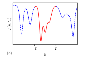
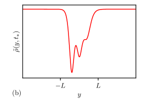
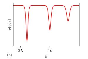
Let be a realization of a soliton gas solution to the dispersive hydrodynamics (4) and let be defined in such a way that for some one has for and outside of this interval. To avoid complications we assume that the transition between the two behaviors is smooth but sufficiently rapid so that such a “windowed” portion of a soliton gas (see Fig. 3) can be approximated by -soliton solution of (4) for some , with the discrete IST spectrum being distributed on and with densities and respectively (recall the definition of DOS in Sec. I). Equation (20) rewrites
| (21) |
We note the integral (21) does not depend on time because is a conserved quantity, in particular, for where the solution asymptotically represents the train of spatially well-separated solitons propagating on the background (see Fig. 3). In this case, can be evaluated as
| (22) |
where are the spectral parameters and the initial phases of the -solitons. Since the spectrum is preserved by the integrable dynamics (4), remain to be distributed on with the respective densities for all . Let be the “mass” of the spectral soliton solution ,
| (23) |
which only depends on . Note that the integral in (23) converges for the example considered in Sec. II.3 since decays exponentially to . We have with this new notation: . Taking the continuous limit, and , we obtain:
| (24) |
yielding the expression for the moment :
| (25) |
Similarly, we obtain for the two other moments (recall that we assume as ):
| (26) | ||||
| (27) |
where and . The expressions (III), (III) and (III) rewrite in the isotropic case:
| (28) |
We present in Table 1 the expressions of , and for the examples introduced in Sec. II.3.
| equations | |||
|---|---|---|---|
| DNLS () | |||
| RNLS () |
The method presented here only requires to integrate the single-soliton solution and thus can be readily applied to any integrable dispersive hydrodynamic system supporting the soliton resolution scenario. Formulas (III), (III), (III) and (28) will be used in the next section to track the evolution of the DOS numerically. In conclusion we note that the above simple method, applied to the KdV equation, gives exactly the same results for the mean and mean square of the random field as the finite-gap theory consideration of el_thermodynamic_2003 ; el_critical_2016 . It also explains why the corresponding analytical expressions for the moments in a dense gas of KdV solitons derived in el_critical_2016 coincide with the corresponding expressions obtained in dutykh_numerical_2014 for a rarefied gas (see also shurgalina_nonlinear_2016 for the similar modified KdV equation result).
In the above consideration of homogeneous soliton gases the ensemble averages (19) are constant. For a nonhomogeneous gas the DOS is a slowly varying function of and so are the ensemble averages that now need to be interpreted as “local averages” in the spirit of modulation theory whitham_linear_1999 . Essentially, one introduces a mesoscopic scale , much larger than the typical soliton width and much smaller than the spatial scale of the DOS variations so that the DOS is approximately constant on any interval . Then the constant ensemble averages (19) are replaced by slowly varying quantities:
| (29) |
The local averages do not depend on at leading order, and their spatiotemporal variations occur on -scales that correspond to the scales associated with variations of and are much larger than those of , . The modulations of , and in a nonhomogeneous soliton gas are then defined by the equations (III), (III) and (III) respectively, in which the DOS is replaced by the solution of the kinetic equation (6),(7). This strategy will be used in the next section where we study dynamics of nonhomogeneous soliton gases generated in the solutions of Riemann problems for kinetic equations.
IV Multi-component bidirectional soliton gases: Riemann problem
IV.1 Hydrodynamics reductions
Generally, our ability to solve the integral equation of state (I) is very limited, and strongly depends on the particular form of the interaction kernel. Some particular analytical solutions have been found el_spectral_2020 for special cases of soliton gases for the focusing NLS equation. At the same time, it was shown in el_kinetic_2005 ; el_kinetic_2011 ; pavlov_generalized_2012 that this problem greatly simplifies if discretization the DOS or with respect to the soliton spectral parameter is admissible. We adopt this simplification in the following, and we consider the soliton gases that are composed of a finite number of distinct spectral components, termed monochromatic, or cold, components. We consider in the following the general anisotropic description; the derivation also readily applies to the isotropic case. Suppose that the bidirectional soliton gas is spectrally composed of distinct components of the “” soliton branch, and distinct components of the “” soliton branch:
| (30) |
with and where are the soliton parameters of the different components and the Dirac delta distribution. We do not indicate in the following the branch-belonging of the component for readability reason. Additionally, we do not indicate explicitly the -dependence of the fields when it is clear. As pointed out in carbone_macroscopic_2016 ; el_spectral_2020 , the multi-component ansatz (30) is a mathematical idealization, physically one would replace the -functions by narrow distributions around the spectral points .
The ansatz (30) transforms the pair of distributions into a -dimensional vector . Thus (6) reduces to hydrodynamic (quasi-linear) conservation laws:
| (31) |
where with indicating the branch-belonging of the soliton . The coupled equations of states (7) simplify into a th-order linear algebraic system for the ’s:
| (32) |
The system (32) simplifies for the examples considered in Sec. II.3, where we assumed that and where the phase shift formula has the form: ; the expression of is given by (11) for the DNLS and (15) for the RNLS equation. For the NLS examples we obtain the linear system:
| (33) |
In order to simplify the discussion, we will focus on the latter system. Both anisotropic and isotropic soliton gases are described by the same system (31),(33): for the isotropic DNLS-soliton gas we have , and for the anisotropic RNLS-soliton gas .
The resolution of the linear system (33) yields a solution such that the system (31) becomes quasi-linear:
| (34) |
It was shown in el_kinetic_2011 ; pavlov_generalized_2012 that the system (34) is a linearly degenerate integrable system ferapontov_integration_1991 and its general solutions can be obtained using the generalized hodograph method tsarev_geometry_1991 . In particular, the characteristic velocities of this hydrodynamic system coincide with the mean velocities .
IV.2 Shock-tube problem
We now focus on the physically relevant Riemann problem for the hydrodynamic system (33),(34) describing the interaction dynamics of two soliton gases prepared in the respective uniform states and , that are initially separated:
| (36) |
The spectral distribution (36) corresponds to the soliton gas “shock tube” problem, an analog of the standard shock tube problem of classical gas dynamics. The shock tube problem represents a good benchmark for our kinetic theory where we can investigate both overtaking and head-on collisions by choosing the appropriate number of components. We emphasize here that the initial condition (36) constitutes a Riemann problem for the kinetic equation (34) but not for the original dispersive hydrodynamics system (4), similar to the so-called generalized Riemann problems recently introduced in sprenger_discontinuous_2020 ; gavrilyuk_stationary_2020 . We shall sometimes refer to the problem (34),(36) as a “spectral Riemann problem” as it essentially describes the spatiotemporal evolution of the spectral components of the soliton gas.
The soliton gas shock tube problem has been investigated for the KdV and focusing NLS two-component soliton gases () in el_kinetic_2005 ; carbone_macroscopic_2016 ; el_spectral_2020 , and for components in the context of generalized hydrodynamics castro-alvaredo_emergent_2016 ; bertini_transport_2016 ; doyon_dynamics_2017 ; kuniba_generalized_2020 ; croydon_generalized_2020 . Here we present the problem for the -component bidirectional anisotropic soliton gases. An important difference of our consideration from the generalized hydrodynamics setting is that we are interested not only in the spectral characterization of soliton gases via solutions of the kinetic equations but also (and ultimately) in the description of the classical nonlinear wave fields associated with these solutions. The latter is achieved by the evaluation of the ensemble averages as described in Section III.
Due to the scaling invariance of the problem (the kinetic equation (34) and the initial condition (36) are both invariant with respect to the transformation , ), the solution is a self-similar distribution . Because of the linear degeneracy of the quasi-linear system (34) the only admissible solutions are constant separated by contact discontinuities, cf. for instance rozhdestvenskii_systems_1983 . Discontinuous, weak, solutions are physically acceptable here since the kinetic equation describes the conservation of the number of solitons within any given spectral interval, and Rankine-Hugoniot type conditions can be imposed to ensure the conservation of the number of solitons across discontinuities. The solution of the Riemann problem is composed of constant states, or plateaus, separated by discontinuities (see e.g. lax_hyperbolic_1973 ):
| (37) |
where the index indicates the -th component of the vector , and the exponent the index of the plateau. For clarity we labeled the superscripts as “L” (left boundary condition) and as “R” (right boundary condition). Additionally the index of the plateau’s value will be written as a Roman numeral in the examples considered later on. The contact discontinuities propagate at the characteristic velocities lax_hyperbolic_1973 :
| (38) |
where the plateaus’ values are given by Rankine-Hugoniot jump conditions:
| (39) | ||||
| (40) |
where . The Rankine-Hugoniot conditions with are trivially satisfied by the definition of contact discontinuity (38). Recalling the effective derivation of the equation of state in Sec. II.2, the velocity of the contact discontinuity can be identified as the velocity of a trial soliton with parameter propagating in a soliton gas of density or equivalently .
Note that, if the solitons were not interacting, the initial step distribution for the component would have propagated at the free soliton velocity :
| (41) |
which dramatically differs from the solution (37). In order to demonstrate the validity of the solution (37),(38),(39) the Riemann problem is investigated numerically for the DNLS and RNLS equations for two- and three-component soliton gases in the next sections.
IV.2.1 Two-component soliton gas
We consider in this section the interaction between two components of soliton gas with respective parameters and (recall that ). The solution of the equation of state (33) reads for :
| (42) |
As noted in el_kinetic_2005 , the densities and must satisfy the inequality:
| (43) |
for the expressions (42) to remain valid; we suppose that this condition is always verified, constraining the DOS in the following. We suppose that and : the region is initially only populated with -solitons and the region of slower -solitons. Since the two “species” of soliton are interacting. Note that (43) implies . The solution (37) has 3 plateaus:
| (44) |
where , with the value at the intermediate plateau:
| (45) |
and the velocities of the discontinuities:
| (46) |
Both kinds of soliton propagate in the region delimited by and (since , ), and we refer to this region as the interaction region in the following. The discontinuity’s velocity corresponds to the effective velocity of solitons in this region. The total density of solitons in the interaction region is given by:
| (47) |
If () then the total density is smaller (larger) than the sum of the initial soliton densities , and (), cf. for instance el_kinetic_2005 .
The two-component shock tube problem () has been investigated numerically in carbone_macroscopic_2016 for KdV soliton gases. We have shown in Sec. II.3 that the kinetic dynamics of the KdV soliton and the isotropic DNLS soliton gas are both governed by equations (1),(II.3) with . Thus solutions of the DNLS spectral Riemann problem and the KdV spectral Riemann problem are expected to describe very similar dynamics, and we rather focus on the anisotropic RNLS soliton gas exhibiting two distinct kinds of interaction. The solution of the RNLS spectral Riemann problem is given by (44),(45),(46) where with defined in (15).
To verify the validity of our spectral solutions in the context of the original nonlinear wave problem of the interaction of soliton gases, we solve numerically the RNLS equation (13) with initial conditions corresponding to the spectral Riemann data (36) for two different RNLS soliton gases with: (i) overtaking collisions (), and (ii) head-on collisions (). The boundary values and for cases (i) and (ii) are indicated in Table 2. initial conditions are realized according to the initial step distribution (36) and evolved through a direct numerical simulation of the NLS equation (8) with . The details of the numerical implementation of the initial condition (36) and the direct numerical resolution of (8) are given in Appendix B.
| soliton parameter | left boundary condition | right boundary condition | |
|---|---|---|---|
| (i) | |||
| (ii) | |||
| (iii) | |||
| (iv) |
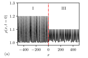
A typical RNLS soliton gas distribution and its corresponding numerical evolution are displayed in Fig. 4 for the spectral Riemann problem (i); soliton gas realizations for the spectral Riemann problem (ii) have a similar variation with different velocities and . We emphasize that, although the soliton gas is initially prepared in a rarefied regime where solitons are spatially well-separated (cf. Appendix B), the total density of solitons increases in the interaction region, and a dense soliton gas can be observed in Fig. 4 for which solitons exhibit significant overlap.
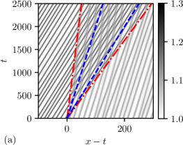
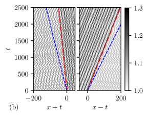
Spatiotemporal evolution of one soliton gas realization is displayed in Fig. 5, with overtaking collisions (i) and head-on collisions (ii). To enhance the discrepancy between free soliton velocities and contact discontinuities velocity the trajectories of the solitons are followed in the frames for overtaking collisions where , and for head-on collisions where and . One can notice that the interaction time between two solitons is very short for a head-on collision, which explains the weakness of head-on interactions compared to overtaking interactions.

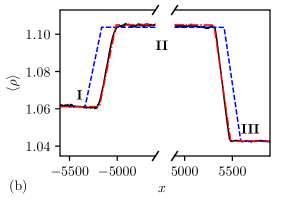
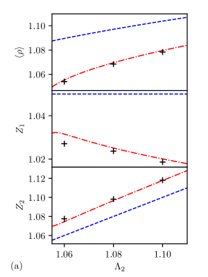
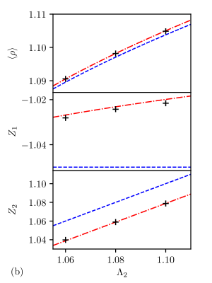
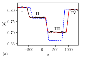
The averaging of the numerical solutions yields the statistical moments of the nonlinear wave fields of the RNLS dispersive hydrodynamics. Fig. 6 displays the comparison between obtained numerically and the analytical solution (35),(44) for (i) and (ii). Note that the discontinuities in have a finite slope in Fig. 6 which is an artifact of the averaging procedure detailed in Appendix B. The comparison between the numerical values of , , fitted from the numerical solution , and the analytical solutions (45),(46) for different values of is displayed in Fig. 7. The comparison shows a good agreement between analytical and numerical solutions and highlights the contrasting effects of (i) overtaking and (ii) head-on collisions. As predicted in the case (i), whereas in the case (ii). In the case (ii) in the region of interaction is almost equal to the average value of for a non-interacting soliton gas (cf. solution (41)). This is due to the weakness of the head-on interaction, clearly displayed in the comparison between and in Fig. 1.
The discrepancy between the analytical and numerical solutions can be associated to the numerical implementation and the time-evolution of the soliton gas. The construction of the soliton gas at , detailed in Appendix B.1, is only valid if the overlap between solitons is negligible, which is not exactly the case for the parameters considered in Table 2. Since is the typical width of the -soliton, the overlap between solitons becomes more important as decreases for a fixed initial density . Besides the numerical scheme utilized to solve the RNLS equation is only valid for small amplitude solitons, cf. Appendix B.2, and the discrepancy also increases as increases.
Additionally, we can compute the variation of the components and of the DOS using the expression (35):
| (48) |
providing that the determinant does not vanish. In particular, we can evaluate numerically the total density from the numerical solutions. Fig. 8 displays the comparison of the total density corresponding to the examples presented in Fig. 6. Notice that, since with , the variation of the moment and the variation of the total density are qualitatively similar. As expected the RNLS soliton gas rarefies when solitons interact with overtaking collisions (), and condenses with head-on collisions (). As pointed out previously, the total density in the example (ii) is very close to the total density of the non-interacting gas because of the weakness of the phase shift induced by head-on collisions.
IV.2.2 Three-component gas
We consider now the case of three-component gases with one component belonging to the slow spectral branch and two components belonging to the fast branch for: (iii) the DNLS equation, (iv) the RNLS equation. Note that in the latter case the anisotropic soliton gas features both overtaking collisions and head-on collisions. Although one can formally solve the equation of state (33) to obtain the expression of and solve the Rankine-Hugoniot condition (39), the analytical expressions do not read as easily as the expressions obtained in the two-component case. We choose here to solve (33),(39) numerically. The values and of the initial soliton densities considered numerically are indicated in Table 2.
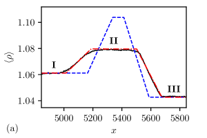
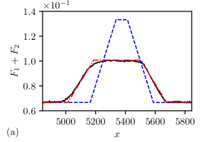
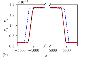
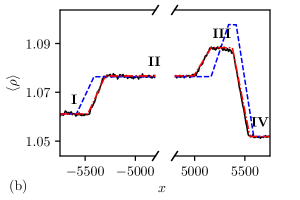
initial conditions are realized according to the initial spectral step distribution (36) and evolved through a direct numerical simulation of the NLS equation (8). The statistics of the soliton gas is then obtained by computing the average from the evolution of the realizations. Fig. 9 displays the variation of the statistical moment . As expected, the solution is composed of 4 plateaus, where regions II and III contain at least two distinct soliton components and are region of interactions. The comparison in Fig. 9 shows a good agreement between the analytical solution (35),(41) and the statistical averages of the numerical solutions.
V Conclusions and Outlook
In this work we have developed the spectral kinetic theory of soliton gases in bidirectional integrable dispersive hydrodynamic systems. Previously, such theory had been developed for (effectively) unidirectional soliton gases, in which all pairwise soliton collisions are characterized by a single expression for the phase shift. Generally, however, the phase shifts in the overtaking and head-on collisions of solitons are essentially different, which necessitates the extension of the existing theory to bidirectional case. This extension is also motivated by the recent experimental results on the generation of bidirectional shallow water soliton gases redor_experimental_2019 ; redor_analysis_2020 .
The definitive quantitative characteristics of an integrable soliton gas is the density of states (DOS), which is the density function in the spectral (IST) -phase space. The DOS evolution in a unidirectional non-uniform soliton gas is governed by the kinetic equation consisting of the continuity equation (1) complemented by the integral equation of state (I) relating the soliton gas velocity and the DOS. The presence of two distinct species of solitons corresponding to the slow and fast branches of the dispersion relation in bidirectional systems naturally calls for the introduction of two respective DOS’s. As a result, one arrives at a system of two coupled kinetic equations which is the subject of the present work.
We introduced the notion of isotropic and anisotropic bidirectional soliton gases based on the sign properties of the phase shifts in overtaking and head-on soliton collisions in a bidirectional gas. In the anisotropic case, where the distinction between overtaking and head-on soliton collisions is genuine, the kinetic of the gas is governed by two coupled equations (6),(7) which we obtained using an extension of the direct physical approach proposed in el_kinetic_2005 . The approach of el_kinetic_2005 combines the qualitative ideas of the original Zakharov’s paper zakharov_kinetic_1971 with the mathematical developments of el_thermodynamic_2003 based on the spectral finite-gap theory. In the isotropic case, the coupled system (6),(7) reduces to a single kinetic equation (1),(I) making a bidirectional isotropic gas effectively equivalent to a unidirectional gas.
To highlight the principal differences between isotropic and anisotropic soliton gases we have considered two prototypical physically relevant examples: the (isotropic) soliton gas of the classical defocusing NLS (DNLS) equation (9) and the (anisotropic) soliton gas of the so-called resonant NLS (RNLS) equation (13) having applications in dispersive magneto-hydrodynamics gurevich_origin_1988 ; lee_resonant_2007 . The results for the RNLS equation are also extended to the Kaup-Boussinesq (KB) system (18) describing bidirectional shallow water waves.
To provide connection between the spectral kinetics of soliton gases and the dynamics of the physical parameters of the associated nonlinear wave fields, we have developed a general simple procedure enabling the evaluation of the basic ensemble averages of the soliton gas wave field in terms of the appropriate moments of the spectral DOS.
As an application of the developed kinetic theory we have considered the generalized Riemann (shock-tube) problem describing collision of several monochromatic soliton beams, each consisting of solitons with nearly identical spectral parameters. The interaction dynamics of such beams is described by certain exact hydrodynamic reductions of the spectral kinetic equations. We constructed the weak solutions of the these hydrodynamic reductions in the form of a system of constant states separated by propagating contact discontinuities satisfying appropriate Rankine-Hugoniot conditions. The obtained general solutions were then applied to the description of collisions of DNLS and RNLS soliton gases, and the comparison with direct numerical simulations of the DNLS and RNLS equation was made.
We stress that, although our derivation of the kinetic equation (6),(7) for a dense bidirectional soliton gas is based on the phenomenological method of el_kinetic_2005 , it can be formally justified using the thermodynamic limit of the modulation equations, that has been developed for the KdV and focusing NLS equations in el_thermodynamic_2003 ; el_spectral_2020 and can be readily generalized to other integrable systems supporting finite-gap solutions associated with hyperelliptic spectral Riemann surfaces. Such a mathematical justification will be the subject of a separate work. Meanwhile, the excellent agreement of the exact solutions of the Riemann problems for bidirectional kinetic equation with appropriate direct numerical simulations for the DNLS and RNLS equations provides a convincing confirmation of the validity of our results.
Despite the consideration of this work being formally reliant on the integrability of the nonlinear wave dynamics (4), the developed kinetic theory can be extended to non-integrable systems supporting solitary wave solutions that exhibit nearly elastic collisions. An experimentally accessible example of such physical system (albeit for a unidirectional case) is the so-called viscous fluid conduit equation describing the dynamics of the interface between two immiscible viscous fluids with high density and viscosity contrast ratios, the lighter fluid being buoyantly ascending through the heavier fluid forming a liquid “pipe”, a conduit lowman_dispersive_2013 . This system supports solitary wave solutions that exhibit nearly elastic collisions as demonstrated numerically and confirmed experimentally lowman_interactions_2014 . Constructing kinetic theory of soliton gases for non-integrable Eulerian dispersive hydrodynamic systems of this type represents a challenging open problem.
Another important direction of further research is the extension of the developed kinetic theory to perturbed integrable systems. In particular, kinetic theory of soliton gas for the perturbed DNLS equation could be used to describe soliton gas in a quasi-1D repulsive BEC in a trapping potential, which has been observed experimentally in hamner_phase_2013 . The dynamics of the trapped condensate is governed by the celebrated Gross-Pitaevskii equation, which is the DNLS equation supplemented by an external potential term, which could be treated as a perturbation in certain configurations. Although some properties of a rarefied soliton gas in a trapped BEC have been studied in the previous works schmidt_non-thermal_2012 ; wang_transitions_2015 , the description of a dense gas is not available at present. The investigation of dense soliton gas dynamics in BECs can shed new light on turbulence in superfluids, or “quantum turbulence”, which has been the subject of intense research in recent decades, see e.g. barenghi_introduction_2014 and references therein.
The direct experimental verification of the developed theory could be made possible by the recent advances in the spectral synthesis of soliton gases with a prescribed DOS suret_nonlinear_2020 . While the method of suret_nonlinear_2020 was developed for deep water waves, its extension to other types of wave propagation well described by integrable or nearly integrable systems looks a very promising direction since the kinetic description of soliton gases is achieved essentially in spectral terms.
Concluding, we hope that our work will provide further motivation for the theoretical and experimental study of soliton gases.
Acknowledgments
The work was partially supported by EPSRC grant EP/R00515X/2 (T.C. and G.E.) and DSTL grant DSTLX-1000116851(G.E. and G.R.). The authors thank S. Randoux, P. Suret and A. Tovbis for numerous stimulating discussions.
Appendix A Soliton solution of the KB system
The soliton solution (14) of the RNLS equation reads after substitution in (17):
| (49) |
where . Note that the solution (51) is not centered at but with
| (50) |
The centered soliton solution reads:
| (51) |
which coincides with the solution derived in zhang_bidirectional_2003 .
Appendix B Numerical implementation of soliton gases for the NLS equation
B.1 Implementation of the step distribution
We implement the soliton gas using the method developed in carbone_macroscopic_2016 . The initial step distribution of the spectral Riemann problem (36) with values given in Table 2 describes a rarefied gas where solitons do not overlap. Such a distribution is implemented by the superposition of solitons
| (52) |
where the ’s are the spectral parameters of the solitons and the ’s their initial position. Although the particles’ position of an “ideal” soliton gas should be distributed according to a Poisson process el_soliton_2001 , this cannot be implemented numerically since the solitons are not allowed to overlap. In our numerics, the distance between two solitons is uniformly distributed in the interval with such that the solitons do not overlap; the total density of solitons is given by . We choose for the RNLS-Riemann problems (i), (ii) and (iv) and for the DNLS-Riemann problem, cf. Sec. (IV.2).
B.2 Numerical scheme
The DNLS equation , is solved with periodic boundary conditions using a Fourier spectral method. The linear part of the DNLS equation is resolved with an integrating factor and the problem is integrated in time using fourth-order Runge-Kutta method.
Since the dispersive term in the RNLS equation (13) is a nonlinear term in , the RNLS equation is first transformed into the KB equation (18) using the change of variables (17). The KB system is then solved with periodic boundary conditions using a Fourier spectral method (with a fourth-order Runge-Kutta method for the time integration). Eq. (18) displays a short wavelength instability: the amplitude of modes grows exponentially with time for . We thus filter out Fourier modes after each time step. This imposes a constraint on the type of solitons that can be implemented numerically. Indeed, large amplitude solitons populate the short-wavelength Fourier modes which are not taken into account in the numerical scheme. We thus consider in the numerical simulations the solitons for which .
B.3 Spatial and ensemble averages
The statistical moment determined numerically in Sec. IV.2 is obtained with: 1) the average over ensemble of or realizations and 2) a local spatial average over the mesoscopic space interval (cf. (29)):
| (53) |
As pointed out in Sec. III, both averaging procedures are equivalent providing that the soliton gas is locally ergodic. The choice of the value for ensures that the space interval contains at least solitons. Note that the transitions of the numerically evaluated mean field field corresponding to contact discontinuities in the analytical solution have a finite slope proportional to because of the spatial averaging.
References
- (1) G. Biondini, G. El, M. Hoefer, and P. Miller, “Dispersive hydrodynamics: Preface,” Physica D: Nonlinear Phenomena, vol. 333, pp. 1–5, 2016.
- (2) M. D. Maiden, D. V. Anderson, N. A. Franco, G. A. El, and M. A. Hoefer, “Solitonic dispersive hydrodynamics: Theory and observation,” Physical Review Letters, vol. 120, p. 144101, 2018.
- (3) P. Sprenger, M. A. Hoefer, and G. A. El, “Hydrodynamic optical soliton tunneling,” Physical Review E, vol. 97, p. 032218, 2018.
- (4) G. A. El, M. A. Hoefer, and M. Shearer, “Expansion shock waves in regularized shallow-water theory,” Proceedings of the Royal Society A: Mathematical, Physical and Engineering Sciences, vol. 472, p. 20160141, 2016.
- (5) G. A. El and M. A. Hoefer, “Dispersive shock waves and modulation theory,” Physica D: Nonlinear Phenomena, vol. 333, pp. 11–65, 2016.
- (6) V. E. Zakharov, “Turbulence in integrable systems,” Studies in Applied Mathematics, vol. 122, pp. 219–234, 2009.
- (7) A. V. Gurevich, K. P. Zybkin, and G. A. Él’, “Development of stochastic oscillations in a one-dimensional dynamical system described by the Korteweg-de Vries equation,” Journal of Experimental and Theoretical Physics, vol. 88, pp. 182–195, 1999.
- (8) G. A. El, E. G. Khamis, and A. Tovbis, “Dam break problem for the focusing nonlinear Schrödinger equation and the generation of rogue waves,” Nonlinearity, vol. 29, pp. 2798–2836, 2016.
- (9) P. Walczak, S. Randoux, and P. Suret, “Optical rogue waves in integrable turbulence,” Physical Review Letters, vol. 114, p. 143903, 2015.
- (10) S. Randoux, P. Walczak, M. Onorato, and P. Suret, “Nonlinear random optical waves: Integrable turbulence, rogue waves and intermittency,” Physica D: Nonlinear Phenomena, vol. 333, pp. 323–335, 2016.
- (11) A. A. Gelash and D. S. Agafontsev, “Strongly interacting soliton gas and formation of rogue waves,” Physical Review E, vol. 98, pp. 042210–1–042210–12, 2018.
- (12) A. Costa, A. R. Osborne, D. T. Resio, S. Alessio, E. Chrivì, E. Saggese, K. Bellomo, and C. E. Long, “Soliton Turbulence in Shallow Water Ocean Surface Waves,” Physical Review Letters, vol. 113, p. 108501, 2014.
- (13) S. Trillo, G. Deng, G. Biondini, M. Klein, G. F. Clauss, A. Chabchoub, and M. Onorato, “Experimental observation and theoretical description of multisoliton fission in shallow water,” Physical Review Letters, vol. 117, p. 144102, 2016.
- (14) S. Trillo, M. Klein, G. Clauss, and M. Onorato, “Observation of dispersive shock waves developing from initial depressions in shallow water,” Physica D: Nonlinear Phenomena, vol. 333, pp. 276–284, 2016.
- (15) A. Gelash, D. Agafontsev, V. Zakharov, G. El, S. Randoux, and P. Suret, “Bound state soliton gas dynamics underlying the spontaneous modulational instability,” Physical Review Letters, vol. 123, p. 234102, 2019.
- (16) G. El and A. Tovbis, “Spectral theory of soliton and breather gases for the focusing nonlinear Schrödinger equation,” Physical Review E, vol. 101, p. 052207, 2020.
- (17) G. A. El and A. M. Kamchatnov, “Kinetic equation for a dense soliton gas,” Physical Review Letters, vol. 95, p. 204101, 2005.
- (18) P. Suret, A. Tikan, F. Bonnefoy, F. Copie, G. Ducrozet, A. Gelash, G. Prabhudesai, G. Michel, A. Cazaubiel, E. Falcon, G. El, and S. Randoux, “Nonlinear spectral synthesis of soliton gas in deep-water surface gravity waves,” arXiv:2006.16778 [nlin.PS], 2020.
- (19) G. A. El, A. M. Kamchatnov, M. V. Pavlov, and S. A. Zykov, “Kinetic Equation for a Soliton Gas and Its Hydrodynamic Reductions,” Journal of Nonlinear Science, vol. 21, pp. 151–191, 2011.
- (20) M. J. Ablowitz and Y. Kodama, “Note on asymptotic solutions of the Korteweg-de Vries equation with solitons,” Studies in Applied Mathematics, vol. 66, pp. 159–170, 1982.
- (21) V. E. Zakharov, “Kinetic equation for solitons,” Journal of Experimental and Theoretical Physics, vol. 33, pp. 538–541, 1971.
- (22) G. A. El, “The thermodynamic limit of the Whitham equations,” Physics Letters A, vol. 311, pp. 374–383, 2003.
- (23) G. A. El, “Critical density of a soliton gas,” Chaos: An Interdisciplinary Journal of Nonlinear Science, vol. 26, p. 023105, 2016.
- (24) B. Doyon, T. Yoshimura, and J.-S. Caux, “Soliton Gases and Generalized Hydrodynamics,” Physical Review Letters, vol. 120, p. 045301, 2018.
- (25) B. Doyon, H. Spohn, and T. Yoshimura, “A geometric viewpoint on generalized hydrodynamics,” Nuclear Physics B, vol. 926, pp. 570–583, 2018.
- (26) D.-L. Vu and T. Yoshimura, “Equations of state in generalized hydrodynamics,” SciPost Physics, vol. 6, p. 23, 2019.
- (27) G. B. Whitham, Linear and Nonlinear Waves. John Wiley & Sons, Inc., 1999.
- (28) D. J. Kaup, “A higher-order water-wave equation and the method for solving it,” Progress of Theoretical Physics, vol. 54, pp. 396–408, 1975.
- (29) A. M. Kamchatnov, Nonlinear periodic waves and their modulations: an introductory course. World Scientific, 2000.
- (30) A. G. Abanov, E. Bettelheim, and P. Wiegmann, “Integrable hydrodynamics of calogero–sutherland model: bidirectional benjamin–ono equation,” Journal of Physics A: Mathematical and Theoretical, vol. 42, p. 135201, 2009.
- (31) I. Redor, E. Barthélemy, H. Michallet, M. Onorato, and N. Mordant, “Experimental Evidence of a Hydrodynamic Soliton Gas,” Physical Review Letters, vol. 122, no. 21, p. 214502, 2019.
- (32) I. Redor, E. Barthélemy, N. Mordant, and H. Michallet, “Analysis of soliton gas with large-scale video-based wave measurements,” Experiments in Fluids, vol. 61, p. 216, 2020.
- (33) Y. Li and J. E. Zhang, “Bidirectional soliton solutions of the classical Boussinesq system and AKNS system,” Chaos, Solitons & Fractals, vol. 16, pp. 271–277, 2003.
- (34) V. E. Zakharov and A. B. Shabat, “Interaction between solitons in a stable medium,” Journal of Experimental and Theoretical Physics, vol. 37, pp. 823–828, 1973.
- (35) J.-H. Lee, O. Pashaev, C. Rogers, and W. Schief, “The resonant nonlinear Schrödinger equation in cold plasma physics. application of Bäcklund–Darboux transformations and superposition principles,” Journal of Plasma Physics, vol. 73, pp. 257–272, 2007.
- (36) J. Yang, Nonlinear Waves in Integrable and Nonintegrable Systems. Society for Industrial and Applied Mathematics, 2010.
- (37) M. Schmidt, S. Erne, B. Nowak, D. Sexty, and T. Gasenzer, “Non-thermal fixed points and solitons in a one-dimensional Bose gas,” New Journal of Physics, vol. 14, p. 075005, 2012.
- (38) W. Wang and P. G. Kevrekidis, “Transitions from order to disorder in multiple dark and multiple dark-bright soliton atomic clouds,” Physical Review E, vol. 91, p. 032905, 2015.
- (39) J.-H. Lee and O. K. Pashaev, “Solitons of the resonant nonlinear Schrödinger equation with nontrivial boundary conditions: Hirota bilinear method,” Theoretical and Mathematical Physics, vol. 152, pp. 991–1003, 2007.
- (40) A. V. Gurevich and A. L. Krylov, “The origin of a nondissipative shock wave,” Doklady Physics: A Journal of the Russian Academy of Sciences, vol. 33, no. 8, pp. 603–605, 1988.
- (41) G. A. El, A. L. Krylov, S. Molchanov, and S. Venakides, “Soliton turbulence as a thermodynamic limit of stochastic soliton lattices,” Physica D: Nonlinear Phenomena, vol. 152-153, pp. 653–664, 2001.
- (42) H. Flaschka, M. G. Forest, and D. W. McLaughlin, “Multiphase averaging and the inverse spectral solution of the Korteweg-de Vries equation,” Communications on Pure and Applied Mathematics, vol. 33, pp. 739–784, 1980.
- (43) J. Moser, Integrable Hamiltonian Systems and Spectral Theory. Scuola normale superiore, 1981.
- (44) E. G. Shurgalina and E. N. Pelinovsky, “Nonlinear dynamics of a soliton gas: Modified Korteweg–de Vries equation framework,” Physics Letters A, vol. 380, pp. 2049–2053, 2016.
- (45) D. Dutykh and E. Pelinovsky, “Numerical simulation of a solitonic gas in KdV and KdV–BBM equations,” Physics Letters A, vol. 378, pp. 3102–3110, 2014.
- (46) M. V. Pavlov, V. B. Taranov, and G. A. El, “Generalized hydrodynamic reductions of the kinetic equation for a soliton gas,” Theoretical and Mathematical Physics, vol. 171, pp. 675–682, 2012.
- (47) F. Carbone, D. Dutykh, and G. A. El, “Macroscopic dynamics of incoherent soliton ensembles: Soliton gas kinetics and direct numerical modelling,” EPL (Europhysics Letters), vol. 113, p. 30003, 2016.
- (48) E. Ferapontov, “Integration of weakly nonlinear hydrodynamic systems in Riemann invariats,” Physics Letters A, vol. 158, pp. 112–118, 1991.
- (49) S. P. Tsarëv, “The geometry of hamiltonian systems of hydrodynamic type. the generalized hodograph method,” Mathematics of the USSR-Izvestiya, vol. 37, pp. 397–419, 1991.
- (50) P. Sprenger and M. A. Hoefer, “Discontinuous shock solutions of the whitham modulation equations as zero dispersion limits of traveling waves,” Nonlinearity, vol. 33, pp. 3268–3302, 2020.
- (51) S. Gavrilyuk, B. Nkonga, K.-M. Shyue, and L. Truskinovsky, “Stationary shock-like transition fronts in dispersive systems,” Nonlinearity, vol. 33, pp. 5477–5509, 2020.
- (52) O. A. Castro-Alvaredo, B. Doyon, and T. Yoshimura, “Emergent hydrodynamics in integrable quantum systems out of equilibrium,” Physical Review X, vol. 6, p. 041065, 2016.
- (53) B. Bertini, M. Collura, J. De Nardis, and M. Fagotti, “Transport in out-of-qquilibrium XXZ chains: exact profiles of charges and currents,”, Physical Review Letters, vol. 117, p. 207201, 2016.
- (54) B. Doyon and H. Spohn, “Dynamics of hard rods with initial domain wall state,” Journal of Statistical Mechanics:Theory and Experiment, vol. 7, p. 073210, 2017.
- (55) A. Kuniba, G. Misguich, and V. Pasquier, “Generalized hydrodynamics in box-ball system,” Journal of Physics A: Mathematical and Theoretical, vol. 53, p. 404001, 2020.
- (56) D. A. Croydon and M. Sasada, “Generalized Hydrodynamic Limit for the Box–Ball System,” Communications in Mathematical Physics, 2020.
- (57) B. Rozhdestvenskii and N. Janenko, Systems of quasilinear equations and their applications to gas dynamics. Providence: RI: American Mathematical Society, 1983.
- (58) P. D. Lax, Hyperbolic systems of conservation laws and the mathematical theory of shock waves. Society for Industrial and Applied Mathematics, 1973.
- (59) C. Hamner, Y. Zhang, J. J. Chang, C. Zhang, and P. Engels, “Phase winding a two-component Bose-Einstein Condensate in an elongated trap: experimental observation of moving magnetic orders and dark-bright solitons,” Physical Review Letters, vol. 111, p. 264101, 2013.
- (60) C. F. Barenghi, L. Skrbek, and K. R. Sreenivasan, “Introduction to quantum turbulence,” Proceedings of the National Academy of Sciences, vol. 111, pp. 4647–4652, 2014.
- (61) N. K. Lowman and M. A. Hoefer, “Dispersive hydrodynamics in viscous fluid conduits,” Physical Review E, vol. 88, p. 023016, 2013.
- (62) N. K. Lowman, M. A. Hoefer, and G. A. El, “Interactions of large amplitude solitary waves in viscous fluid conduits,” Journal of Fluid Mechanics, vol. 750, pp. 372–384, 2014.
- (63) J. E. Zhang and Y. Li, “Bidirectional solitons on water,” Physical Review E, vol. 67, p. 016306, 2003.