Algorithmic Reduction of Biological Networks With Multiple Time Scales

Abstract

We present a symbolic algorithmic approach that allows to compute invariant manifolds and corresponding reduced systems for differential equations modeling biological networks which comprise chemical reaction networks for cellular biochemistry, and compartmental models for pharmacology, epidemiology and ecology. Multiple time scales of a given network are obtained by scaling, based on tropical geometry. Our reduction is mathematically justified within a singular perturbation setting. The existence of invariant manifolds is subject to hyperbolicity conditions, for which we propose an algorithmic test based on Hurwitz criteria. We finally obtain a sequence of nested invariant manifolds and respective reduced systems on those manifolds. Our theoretical results are generally accompanied by rigorous algorithmic descriptions suitable for direct implementation based on existing off-the-shelf software systems, specifically symbolic computation libraries and Satisfiability Modulo Theories solvers. We present computational examples taken from the well-known BioModels database using our own prototypical implementations.

1 Introduction

Biological network models describing elements in interaction are used in many areas of biology and medicine. Chemical reaction networks are used as models of cellular biochemistry, including gene regulatory networks, metabolic networks, and signaling networks. In epidemiology and ecology, compartmental models can be described as networks of interactions between compartments. Both in chemical reaction networks and in compartmental models, the probability that two elements interact is assumed proportional to their abundances. This property, called mass action law in biochemistry, leads to polynomial differential equations in the kinetics.

For differential equations that describe the development of such networks over time, a crucial question is concerned with reduction of dimension. We illustrate such a reduction and the steps involved for the classic Michaelis–Menten system, an archetype of enzymatic reactions. This system is described by the chemical reactions

$$\ce{E+S<=>[k_{\_}1][k_{\_}{-1}]ES->[k_{\_}2]E+P},$$

where E, S, ES, and P are the enzyme, substrate, enzyme-substrate complex, and product, respectively. The mechanism has two conserved quantities $\ce{[E]}+\ce{[ES]}=c_{\_}1$ and $\ce{[S]}+\ce{[ES]}+\ce{[P]}=c_{\_}2$, where $c_{\_}1$ and $c_{\_}2$ are constant functions representing the respective total concentrations. Let us choose the concentration units such that $c_{\_}2=1$, and furthermore rename $c_{\_}1=\varepsilon$. In the ordinary differential equations describing the kinetics of [E], [S], [ES], and [P] according to [24, Sect. 2.1.2] we eliminate the variable $\ce{[E]}=\varepsilon-\ce{[ES]}$. This yields a reduced system made of variables $y_{\_}1=\ce{[S]}$ and $y_{\_}2=\ce{[ES]}$ as follows:

$$\dot{y_{\_}1} =-\varepsilon k_{\_}1y_{\_}1+(k_{\_}1y_{\_}1+k_{\_}{-1})y_{\_}2$$

$$\dot{y_{\_}2} =\varepsilon k_{\_}1y_{\_}1-(k_{\_}1y_{\_}1+k_{\_}{-1}+k_{\_}2)y_{\_}2.$$

Notice that $\dot{\ce{[P]}}$ is already determined by the algebraic conservation constraint $\ce{[P]}=1-y_{\_}1-y_{\_}2$. The parameter $\varepsilon$ represents the ratio of total concentrations $c_{\_}1$ to $c_{\_}2$. The general idea is that $\varepsilon$ is small.

In a first step toward reduction, a scaling transformation $y_{\_}1=x_{\_}1$ and $y_{\_}2=\varepsilon x_{\_}2$ yields

$$\dot{x_{\_}1} =\varepsilon(-k_{\_}1x_{\_}1+(k_{\_}1x_{\_}1+k_{\_}{-1})x_{\_}2)$$

$$\dot{x_{\_}2} =k_{\_}1x_{\_}1-(k_{\_}1x_{\_}1+k_{\_}{-1}+k_{\_}2)x_{\_}2.$$

In a second step, one uses singular perturbation theory to obtain the famous Michaelis–Menten equation. It consists of two components: First, we obtain a one dimensional invariant manifold given approximately by the quasi-steady state condition $k_{\_}1x_{\_}1-(k_{\_}1x_{\_}1+k_{\_}{-1}+k_{\_}2)x_{\_}2=0$. This considers the fast variable $x_{\_}2$ to be at the steady state and lowers dimension from two to one. Second, we obtain a reduced system for the slow variable:

$$\dot{x_{\_}1}=-\varepsilon\frac{k_{\_}1k_{\_}2x_{\_}1}{k_{\_}1x_{\_}1+k_{\_}{-1}+k_{\_}2}.$$

With our example, we paraphrased the approach in a seminal paper by Heineken et al. [34], which was the first one to rigorously discuss quasi-steady state from the perspective of singular perturbation theory. Realistic network models may have many species and differential equations. Considerable effort has been put into model order reduction, i.e., finding approximate models with a smaller number of species and equations, where the reduced model can be more easily analyzed than the full model [58].

The scaling of parameters and variables by a small parameter $\varepsilon$ and the study of the limit $\varepsilon\to 0$ is central in singular perturbation theory. It is rather obvious that arbitrary scaling transformations are unlikely to provide useful information about a given system. Successful scalings, in contrast, are typically related to the existence of nontrivial invariant manifolds. Applications of scaling rely on the observation that, loosely speaking, any result that holds asymptotically for $\varepsilon\to 0$ remains valid for sufficiently small positive $\varepsilon_{\_}*$, provided some technical conditions are satisfied. To determine scalings of polynomial or rational vector fields that model biological networks, tropical equilibration methods were introduced and developed in a series of papers by Noel et al. [55], Radulescu et al. [59], Samal et al. [63, 62], and others. These methods open a feasible path for biological networks of high dimension. For a given system they provide a list of possible slow-fast systems, which may or may not yield invariant manifolds and reduced equations. Other methods due to Goeke et al. [31], and recently extended to multiple time scales by Kruff and Walcher [40], determine critical parameter values and manifolds for singular perturbation reductions.

The principal purpose of the present paper is to complement scaling with an algorithmic test for the existence of invariant manifolds and the computation of those manifolds along with corresponding reduced systems of differential equations. In the asymptotic limit, methods from singular perturbation theory, principally developed by Tikhonov [74] and Fenichel [25], are available. A recent extension to multiscale systems by Cardin and Teixeira [11] turns out to be a valuable tool for the systematic computation of reductions with nested invariant manifolds and allows an algorithmic approach.

In the language of dynamical systems, the behavior of systems with multiple time scales can be described as follows. All variables evolve towards the steady state of the ordinary differential equation that they follow, but not with the same speed, in other words, not within the same time scale. Slow variables correspond to long time scales, and fast variables correspond to short time scales. The steady state of a subset of the ordinary differential equations is called quasi-steady state, and the evolution of a variable or group of variables towards its quasi-steady state is called relaxation. At a given time scale, a group of variables relaxes towards one of their quasi-steady states. The set of all quasi-steady states of variables relaxing within the same time scale forms a critical manifold, which provides the lowest order approximation to the corresponding invariant manifold. In this article, we do not distinguish between critical and invariant manifolds, since we do not discuss higher order approximations. All slower variables can be considered fixed, and all faster variables have already relaxed and satisfy quasi-steady state conditions. As the number of relaxed variables increases and thus the set of quasi-steady state conditions grows, the respective invariant manifolds get nested so that later manifolds are contained in earlier ones. Local linear approximations of these manifolds were proposed by Valorani and Paolucci [75] using numerical methods based on the local Jacobian. However, to the best of our knowledge, constructive approaches providing nonlinear descriptions of these manifolds and reduced models are still missing.

From a computer science point of view, we propose a novel symbolic computation-based algorithmic workflow for the reduction process outlined above. This includes in particular the automatic verification of certain hyperbolicity conditions required for the validity of the reductions. We restrict ourselves to the case of polynomial differential equations that covers mass action chemical reaction networks and compartmental models. We present a series of algorithms that takes as input a system of polynomial autonomous ordinary differential equations together with numerical information related to the desired coarse graining of the scaling. As output one finally obtains a collection of nested invariant manifolds for the input system, associated with smaller dimensional systems that govern the dynamics on those manifolds. This output establishes the reduced systems discussed above.

The computationally hard parts of our methods are reduced to decision problems in interpreted first-order logic over various theories. It turns out that quantifier alternation can be entirely avoided, so that the Satisfiability Modulo Theories (SMT) framework by Nieuwenhuis et al. [52] can be applied. Several corresponding SMT solvers are freely available and professionally supported [1, 13, 17, 51]. It is remarkable that we arrive with our comprehensive algorithmic work here at SMT sub-problems for several different logics, viz. linear integer arithmetic, linear real arithmetic, and non-linear real arithmetic. The algorithms presented here are suitable for straightforward implementation provided that a symbolic computation library, or computer algebra system, and an SMT solver are available. We created two independent prototypical realizations in software ourselves, one in Python using freely available libraries, and one in Maple.

The plan of the paper is as follows: In Sect. 2.1 we introduce an abstract scaling procedure, which assumes, for given $0<\varepsilon_{\_}*<1$, the existence of families of exponents $c_{\_}{k,J}$ and $d_{\_}k$ for scaling polynomial coefficients and variables, respectively. From the scaled system, higher order terms are truncated, and the obtained system is partitioned into several time scales, ordered from fastest to slowest. A corresponding generic algorithm uses black-box functions $c$ and $d$. In Sect. 2.2, we make precise one possible way to realize $c$ and $d$, based on tropical geometry. So far, our transformations are mostly of formal nature. On these grounds, we algorithmically determine in Sect. 3 invariant manifolds and corresponding reduced systems, which makes the formal scaling meaningful in a mathematically precise way. In general, this is possible only for a certain number $\ell$ of time scales, where $\ell$ is explicitly found and—in contrast to existing alternative approaches—often larger than $2$. Technically, we apply recent results by Cardin and Teixeira [11] based on Fenichel theory. In Sect. 4, we employ symbolic computation techniques, specifically Gröbner basis theory, to equivalently simplify our reduced systems, which are still scaled in terms of $\varepsilon_{\_}*$, $c$, and $d$. In Sect. 5, we finally transform back to the principal scale of the original system while preserving the obtained multiple time scales and the structure of the corresponding reduced systems. In particular, the various time scale factors remain explicit. In Sect. 6, we summarize what we have gained from the overall procedure for our original input. At this point, the mathematical development of our framework has been accompanied by nine algorithms, and we give a tenth top-level algorithm, which makes precise how various modules are combined and interact with one another. In Sect. 7 we discuss computational examples with our prototypical software mentioned above. We consider models from the BioModels database, a repository of mathematical models of biological processes [57]. The focus is on successful reductions for biologically interesting examples. This is counterbalanced in Appendix A by further examples to support the understanding of our algorithms. This also provides some examples where we do not obtain meaningful reductions. In Sect. 8 we highlight some computational steps in our algorithms from the point of view of asymptotic worst-case complexity. In Sect. 9, we wrap up and point at possible future research directions.

2 Scaling of Polynomial Vector Fields

In what follows, we adopt a rather general scaling formalism that has been used recently in [54, 55, 58, 59, 63] and is recurrent in the literature on singular perturbations, see for instance [53, Sect. 3]. We use the convention that the natural numbers $\mathbb{N}$ include $0$.

2.1 An Abstract Scaling Procedure

Our starting point is a parameter dependent system $S$ of polynomial differential equations

$$\dot{y_{\_}k}:=\frac{\operatorname{d}\!{y_{\_}k}}{\operatorname{d}\!{t}}=\sum_{\_}J\gamma_{\_}{k,J}y^{J},\quad 1\leq k\leq n,$$ (1)

where the summation ranges over multi-indices $J=(j_{\_}1,\ldots,j_{\_}n)\in\mathbb{N}^{n}$, $\gamma_{\_}{k,J}\in\mathbb{R}$, and only finitely many $\gamma_{\_}{k,J}$ are non-zero. We abbreviate $y^{J}=y_{\_}1^{j_{\_}1}\cdots y_{\_}n^{j_{\_}n}$, as usual. In terms of network models, $y_{\_}k$ represents the concentration of either a chemical species or a type of individual in a compartment. Note that we use positive integers as indices, instead of concrete names for species and compartments. The real coefficients $\gamma_{\_}{k,J}$ describe actions of other species or individuals on the species or individual $k$. If these actions are activations one has $\gamma_{\_}{k,J}>0$, whereas for repressions one has $\gamma_{\_}{k,J}<0$. Several species may interact to produce an action on a given species $k$. This information is contained in the number of non-zero components of $J$, which is called the order of the action. This terminology is inspired from chemical reactions, where the order represents essentially the number of reactant species.

Throughout this paper, we require that positive $y_{\_}k$ remain positive as time progresses. In other words, the positive first orthant $\mathcal{U}=(0,\infty)^{n}\subseteq\mathbb{R}^{n}$ is positively invariant for system (1), which is the case, e.g., in chemical reaction networks when $\gamma_{\_}{k,J}y^{J}\geq 0$ on all intersections of hyperplanes $\{\,(y_{\_}1,\dots,y_{\_}n)\in\mathbb{R}^{n}\mid y_{\_}k=0\,\}$ with $\overline{\mathcal{U}}$.

We fix some small $\varepsilon_{\_}*\in(0,1)$, and we impose that

$$\gamma_{\_}{k,J}=\varepsilon_{\_}*^{c_{\_}{k,J}}\bar{\gamma}_{\_}{k,J},$$ (2)

with rational numbers $c_{\_}{k,J}$. The tacit understanding is that only nonzero $\gamma_{\_}{k,J}$ are being considered. The intuitive idea, which will be made more precise in Sect. 2.2, is that the $\bar{\gamma}_{\_}{k,J}$ are close to one. Moreover, we introduce a positive parameter $\varepsilon$ and consider the system

$$\dot{y_{\_}k}=\sum_{\_}J\varepsilon^{c_{\_}{k,J}}\,\bar{\gamma}_{\_}{k,J}\,y^{J},\quad 1\leq k\leq n,$$ (3)

with $\varepsilon$-dependent coefficients. Notice that (3) matches (1) at $\varepsilon=\varepsilon_{\_}*$. By renormalizing $y_{\_}k=\varepsilon^{d_{\_}k}x_{\_}k$, $d_{\_}k\in\mathbb{Q}$, one obtains a system in scaled variables

$$\dot{x_{\_}k}=\sum_{\_}J\varepsilon^{c_{\_}{k,J}+\left<D,J\right>-d_{\_}k}\,\bar{\gamma}_{\_}{k,J}\,x^{J},\quad 1\leq k\leq n,$$ (4)

with $D=(d_{\_}1,\ldots,d_{\_}n)$ and the dot product in $\mathbb{R}^{n}$ denoted by $\left<\cdot,\cdot\right>$. This transformation preserves the positive invariance of $\mathcal{U}$. The scaling comes with the implicit assumption that for $i$, $j\in\{1,\dots,n\}$, the relative order of $y_{\_}i$ with respect to $y_{\_}j$ is bounded by $y_{\_}i/y_{\_}j=\Theta(\varepsilon^{d_{\_}i-d_{\_}j})$ for $\varepsilon\to 0$, so that all $x_{\_}k$ get the same order of magnitude. Continuing, we set $\nu_{\_}k=\min\{\,c_{\_}{k,J}+\left<D,J\right>-d_{\_}k\mid\bar{\gamma}_{\_}{k,J}\not=0\,\}$ to obtain

$$\dot{x_{\_}k}=\varepsilon^{\nu_{\_}k}\sum_{\_}J\varepsilon^{c_{\_}{k,J}+\left<D,J\right>-d_{\_}k-\nu_{\_}k}\,\bar{\gamma}_{\_}{k,J}\,x^{J},\quad 1\leq k\leq n,$$ (5)

where now all exponents of $\varepsilon$ inside the sums are nonnegative. Finally one may perform a preliminary time scaling $\tau=\varepsilon^{\mu}t$, $\mu=\min\,\{\nu_{\_}1,\ldots,\nu_{\_}n\}$ to arrive at

$$x_{\_}k^{\prime}:=\frac{\operatorname{d}\!{x_{\_}k}}{\operatorname{d}\!{\tau}}=\varepsilon^{\nu_{\_}k-\mu}\sum_{\_}J\varepsilon^{c_{\_}{k,J}+\left<D,J\right>-d_{\_}k-\nu_{\_}k}\,\bar{\gamma}_{\_}{k,J}\,x^{J},\quad 1\leq k\leq n,$$ (6)

with all exponents nonnegative. We are interested in system (6) for variable $\varepsilon>0$, in the asymptotic limit $\varepsilon\to 0$.

We restructure (6) by collecting all variables with equal $\nu_{\_}i-\mu$ in vectors $z_{\_}1$, …, $z_{\_}m$, where $z_{\_}k\in\mathbb{R}^{n_{\_}k}$ for $k\in\{1,\dots,m\}$, in ascending order of exponents and such that $n_{\_}1+\dots+n_{\_}m=n$. We obtain a system of the form

$$z_{\_}k^{\prime}=\varepsilon^{a_{\_}k}\widetilde{f}_{\_}k(z,\varepsilon)=\varepsilon^{a_{\_}k}\left(\widetilde{f}_{\_}k(z,0)+\varepsilon^{a_{\_}{k,2}^{\prime}}p_{\_}{k,2}+\cdots+\varepsilon^{a_{\_}{k,w_{\_}{k}}^{\prime}}p_{\_}{k,w_{\_}{k}}\right)=\varepsilon^{a_{\_}k}\left(\widetilde{f}_{\_}k(z,0)+o(1)\right),\quad 1\leq k\leq m,$$ (7)

where $a_{\_}k$, $a_{\_}{k,j}^{\prime}\in\mathbb{Q}$, $0=a_{\_}1<a_{\_}2<\ldots<a_{\_}m$, $0<a_{\_}{k,j}^{\prime}$, and $p_{\_}{k,j}$ are multivariate polynomials in $z$ for $1\leq k\leq m$ and $2\leq j\leq w_{\_}k$. Note that the case $m=1$ is not excluded. By substituting $\delta:=\varepsilon^{1/q}$ with a sufficiently large positive integer $q$, one ensures that only nonnegative integer powers of $\delta$ appear:

$$z_{\_}k^{\prime}=\delta^{b_{\_}k}\widehat{f}_{\_}k(z,\delta)=\delta^{b_{\_}k}\left(\widehat{f}_{\_}k(z,0)+\delta^{b_{\_}{k,2}^{\prime}}p_{\_}{k,2}+\cdots+\delta^{b_{\_}{k,w_{\_}{k}}^{\prime}}p_{\_}{k,w_{\_}{k}}\right)=\delta^{b_{\_}k}\left(\widehat{f}_{\_}k(z,0)+o(1)\right),\quad 1\leq k\leq m,$$ (8)

where $b_{\_}k$, $b_{\_}{k,j}^{\prime}\in\mathbb{N}$, $0=b_{\_}1<b_{\_}2<\ldots<b_{\_}m$, $0<b_{\_}{k,j}^{\prime}$ for $1\leq k\leq m$ and $2\leq j\leq w_{\_}k$.

Our idea is that the indices $k$ correspond to different time scales $\delta^{b_{\_}k}\tau$. For $m>1$, system (8), as $\delta\to 0$, may be thought of as separating fast variables from increasingly slow ones. It will turn out in Sect. 3 that the exact number of time scales finally obtained by our overall approach can actually be smaller than $m$.

Given certain conditions, which will be made explicit in Theorem 1 and with its application in Sect. 3.1, we may formally truncate the right hand sides of (8) and keep only terms of lowest order in $\delta$:

$$z_{\_}k^{\prime}=\delta^{b_{\_}k}\widehat{f}_{\_}k(z,0),\quad 1\leq k\leq m.$$ (9)

In the following, we refer to the transformation process from (1) to (8) as scaling. Strictly speaking, this comprises scaling in combination with partitioning. We refer to the step from (8) to (9) as truncating.

Algorithm 1

Algorithm 1 $\operatorname{ScaleAndTruncate}$

0:  

1. A list $S=\big{[}\frac{\operatorname{d}\!{y_{\_}1}}{\operatorname{d}\!{t}}=f_{\_}1,\dots,\frac{\operatorname{d}\!{y_{\_}n}}{\operatorname{d}\!{t}}=f_{\_}n\big{]}$ of autonomous first-order ordinary differential equations where $f_{\_}1$, …, $f_{\_}n\in\mathbb{Q}[y_{\_}1,\dots,y_{\_}n]$;

2. $c:\{1,\dots,n\}\times\{1,\dots,n\}^{n}\to\mathbb{Q}$;

3. $d:()\to\mathbb{Q}^{n}\cup\{\bot\}$;

4. $\varepsilon_{\_}*\in(0,1)\cap\mathbb{Q}$

0:  

1. A list $[T_{\_}1,\dots,T_{\_}m]$ where, abbreviating $\frac{\operatorname{d}\!{}}{\operatorname{d}\!{\tau}}$ by a prime, $T_{\_}k=(z_{\_}k^{\prime}=\delta^{b_{\_}k}f_{\_}k)$ with $z_{\_}k^{\prime}\subseteq[x_{\_}1^{\prime},\dots,x_{\_}n^{\prime}]$, $\bigcup_{\_}kz_{\_}k^{\prime}=[x_{\_}1^{\prime},\dots,x_{\_}n^{\prime}]$, $z_{\_}1^{\prime}$, …, $z_{\_}m^{\prime}$ pairwise disjoint, $b_{\_}1<\dots<b_{\_}m\in\mathbb{N}$, and $f_{\_}k\subseteq\mathbb{Q}[x_{\_}1,\dots,x_{\_}n]$, or the empty list;

2. A list $[P_{\_}1,\dots,P_{\_}m]$ of lists with $P_{\_}k\subseteq\mathbb{Q}[x_{\_}1,\dots,x_{\_}n][\delta]$ and $|P_{\_}k|=|T_{\_}k|$ for $k\in\{1,\dots,m\}$;

3. A substitution $\sigma$ for $x_{\_}1$, …, $x_{\_}n$, $\tau$, $\delta$, and $\varepsilon$

The first output $[T_{\_}1,\dots,T_{\_}m]$ contains differential equations $z_{\_}k^{\prime}=\delta^{b_{\_}k}\widehat{f}_{\_}k(z,0)$ for $k\in\{1,\dots,m\}$ in terms of system (8). The second output $[P_{\_}1,\dots,P_{\_}m]$ contains the higher order terms in (8) as polynomials $p_{\_}k=\delta^{b_{\_}k+b_{\_}{k,2}^{\prime}}p_{\_}{k,2}+\cdots+\delta^{b_{\_}k+b_{\_}{k,w_{\_}{k}}^{\prime}}p_{\_}{k,w_{\_}{k}}$. The last output is a substitution that undoes all substitutions applied for obtaining (8) from (1).This gives the following invariant: Denote $\widetilde{S}=\bigl{(}\bigcup_{\_}{k=1}^{m}T_{\_}k\oplus P_{\_}k\bigr{)}\sigma$, where $(x^{\prime}=g)\oplus p$ stands for $x^{\prime}=g+p$ and is applied elementwise. Then $\widetilde{S}$ is equal to $S$ up to multiplication of the differential equation $\dot{y_{\_}i}=\sum_{\_}J\gamma_{\_}{i,J}y^{J}$ in $S$ with a positive scalar factor $1/\varepsilon_{\_}*^{\mu+d_{\_}i}$.For $q\in\mathbb{Q}[x_{\_}1,\dots,x_{\_}n](\delta)$ we use $\deg_{\_}\delta(q)$ for the univariate degree of $q$ in $\delta$. Similarly, $\operatorname{tmon}_{\_}\delta(q)$ is the trailing monomial in $\delta$.

1:  if $d()=\bot$ then

2:     return  $[\,]$, $[\,]$, $[\,]$

3:  end if

4:  $\mu:=\infty$

5:  $q:=1$

6:  $(d_{\_}1,\dots,d_{\_}n):=d()$ $\in\mathbb{Q}^{n}$

7:  for $k:=1$ to $n$ do

8:     $h_{\_}k:=0$

9:     for all monomials $\gamma y^{J}$ in $f_{\_}k$ do

10:        $\bar{\gamma}:=\gamma/\varepsilon_{\_}*^{c(k,J)}$ $\in\overline{\mathbb{Q}}$

11:        $\eta:=c(k,J)+\langle(d_{\_}1,\dots,d_{\_}n),J\rangle-d_{\_}k$ $\in\mathbb{Q}$

12:        $\mu:=\min(\mu,\eta)$ $\in\mathbb{Q}$

13:        $q:=\operatorname{lcm}(q,\operatorname{denom}\eta)$ $\in\mathbb{N}\setminus\{0\}$

14:        $h_{\_}k:=h_{\_}k+\varepsilon^{\eta}\bar{\gamma}x^{J}$

15:     end for

16:  end for

17:  for $k:=1$ to $n$ do

18:     $h_{\_}k:=h_{\_}k/\varepsilon^{\mu}$

19:     $h_{\_}k:=h_{\_}k[\varepsilon\leftarrow\delta^{q}]$ $\in\overline{\mathbb{Q}}[x_{\_}1,\dots,x_{\_}n][\delta]$

20:     $g_{\_}k:=\operatorname{tmon}_{\_}\delta h_{\_}k$

21:     $p_{\_}k:=h_{\_}k-g_{\_}k$

22:  end for

23:  $L:=\big{[}\frac{\operatorname{d}\!{x_{\_}1}}{\operatorname{d}\!{\tau}}=g_{\_}1,\dots,\frac{\operatorname{d}\!{x_{\_}n}}{\operatorname{d}\!{\tau}}=g_{\_}n\big{]}$

24:  $[b_{\_}1,\dots,b_{\_}m]:=\operatorname{sort}(\deg_{\_}\delta g_{\_}1,\dots,\deg_{\_}\delta g_{\_}n)$, ascending and removing duplicates

25:  for $k:=1$ to $m$ do

26:     $T_{\_}k:=[\,\frac{\operatorname{d}\!{x}}{\operatorname{d}\!{\tau}}=g\in L\mid\deg_{\_}\delta g=b_{\_}k\,]$

27:     $P_{\_}k:=[\,p_{\_}j\in\{p_{\_}1,\dots,p_{\_}n\}\mid\deg_{\_}\delta g_{\_}j=b_{\_}k\,]$

28:  end for

29:  $\sigma:=[x_{\_}1\leftarrow y_{\_}1/\varepsilon^{d_{\_}1},\dots,x_{\_}n\leftarrow y_{\_}n/\varepsilon^{d_{\_}n}]\circ[\tau\leftarrow\varepsilon^{\mu}t]\circ[\delta\leftarrow\varepsilon^{1/q}]\circ[\varepsilon\leftarrow\varepsilon_{\_}*]$

30:  return  $[T_{\_}1,\dots,T_{\_}m]$, $[P_{\_}1,\dots,P_{\_}m]$, $\sigma$

reflects our discussions so far. It takes as input a list $S$ of differential equations representing system (1) and a choice of $0<\varepsilon_{\_}*<1$ for (2). For our practical purposes, the polynomial coefficients in $S$ as well as $\varepsilon_{\_}*$ are taken from $\mathbb{Q}$. Our algorithm is furthermore parameterized with a function $c$ mapping suitable indices to rational numbers and a constant function $d$ yielding either a tuple $D=(d_{\_}1,\dots,d_{\_}n)$ of rational numbers or $\bot$. The black-box functions $c$ and $d$ reflect the mathematical assumptions around (2) and (4) that suitable $c_{\_}{k,J}$ and $d_{\_}k$ exist, respectively. Suitable instantiations for the parameters $c$ and $d$ can be realized, e.g., using tropical geometry, which will be the topic of the next section. It will turn out that instantiations of $d$ can fail on the given combination of $S$ and $\varepsilon_{\_}*$, which is signaled by the return value $\bot$ of $d$, and checked right away in l.1 of Algorithm 1.

2.2 Scaling via Tropical Geometry

So far, the above transformations leading to (4) are a formal exercise. No particular strategy was applied for choosing $\varepsilon_{\_}*\in(0,1)$. Early model reduction studies used dimensional analysis to obtain $\varepsilon_{\_}*$ as a power product in model parameters [34, 66].

Here we discuss a different approach, based on tropical geometry, also called max-plus or idempotent algebra. This is a relatively recent field of mathematics that draws its origins from fields as diverse as algebraic geometry, optimization, and physics [46]. In all these fields, tropical geometry appears as a technique to simplify non-linear objects. Polynomials are replaced by piecewise-linear functions, and geometrical problems are transformed into combinatorial problems [50].

Tropical geometry is natural for any computation with orders of magnitude. In physics, it occurs as Litvinov–Maslov dequantization of real numbers leading to degeneration of complex algebraic varieties into tropical varieties [45, 77]. The name dequantization originates from the formal analogy between this limiting process and Schrödinger’s dequantization that turns quantum physics into classical physics when the Planck constant is considered a small parameter $\varepsilon$ that tends to zero. Closer, in the physical world, to Litvinov–Maslov dequantization are the vanishing viscosity phenomena, well known in problems of wave propagation. In mathematics, tropical varieties and prevarieties establish a modern tool in the theory of Puiseux series [4].

In contrast to the dimensional analysis approach mentioned above, the value $\varepsilon_{\_}*$ is now not dictated by physico-chemistry. Instead, it is freely chosen to provide “power” parametric descriptions of all the quantities occurring in the differential equations (parameters, monomials, time scales), in a similar way to describing curves by continuously varying real parameters.

Next, we explain how to obtain the orders $c_{\_}{k,J}$ and $D$ introduced in the previous section with (2) and (4), respectively. The orders $c_{\_}{k,J}$ are computed from $\varepsilon_{\_}*\in(0,1)$ and $\gamma_{\_}{k,J}$ as

$$c_{\_}{k,J}=\frac{\operatorname{round}(p\log_{\_}{\varepsilon_{\_}*}|\gamma_{\_}{k,J}|)}{p}.$$ (10)

The function $\operatorname{round}:\mathbb{R}\to\mathbb{Z}$ rounds to nearest, ties to even, in the sense of IEEE 754 [37]. The positive integer $p$ controls the precision of the rounding step. Using $\bar{\gamma}_{\_}{k,J}=\gamma_{\_}{k,J}/\varepsilon_{\_}*^{c_{\_}{k,J}}$ as defined in (2), our definition satisfies the constraint $\varepsilon_{\_}*^{1/(2p)}\leq|\bar{\gamma}_{\_}{k,J}|\leq\varepsilon_{\_}*^{-1/(2p)}$. The orders $D=(d_{\_}1,\dots,d_{\_}n)$ satisfy certain constraints as well. Those constraints result heuristically from the idea of compensation of dominant monomials [54]. Slow dynamics is possible if for each dominant, i.e., much larger than the other, monomial on the right hand side of (6), there is at least one other monomial of the same order but with opposite sign. This condition, named tropical equilibration condition [54, 55, 58, 59, 63, 62], reads

$$\min_{\_}{\gamma_{\_}{k,J}>0}(c_{\_}{k,J}+\left<D,J\right>)=\min_{\_}{\gamma_{\_}{k,J^{\prime}}<0}(c_{\_}{k,J^{\prime}}+\left<D,J^{\prime}\right>).$$ (11)

On these grounds, given system (1), the choice of $\varepsilon_{\_}*$ boils down to defining orders of magnitude. Model parameters are coarse-grained and transformed to orders of magnitude in order to apply tropical scaling. The result depends on which parameters are close and which are very different as dictated by the coarse-graining procedure, i.e., by the choice of $\varepsilon_{\_}*$. Decreasing $\varepsilon_{\_}*$ destroys details, and parameters tend to have the same order of magnitude. Increasing $\varepsilon_{\_}*$ refines details, and parameters range over several orders of magnitude. For instance, using (10) and $p=1$, parameters $k_{\_}1=0.1$ and $k_{\_}2=0.01$ have orders $c_{\_}1=1$ and $c_{\_}2=2$ for $\varepsilon_{\_}*=1/10$ but $c_{\_}1=c_{\_}2=1$ for $\varepsilon_{\_}*=1/50$. This is the perspective taken in [54, 55, 63].

On the one hand, we have just seen that smaller choices of $\varepsilon_{\_}*$ possibly hide details. On the other hand, in the following section we are going to review singular perturbation methods, which provide asymptotic results as a small parameter $\delta$ approaches zero. Following the construction in Sect. 2.1, small choices of $\varepsilon_{\_}*$ lead to small $\delta$, which gives a heuristic argument for choosing $\varepsilon_{\_}*$ rather small. Thus in practice one has to reconcile two competing requirements, which unfortunately, still requires some human intuition.

We are now ready to instantiate the black-box functions $c$ and $d$ in our generic Algorithm 1 with tropical versions as given in Algorithm 2 and Algorithm 3, respectively.

Algorithm 2 $\operatorname{TropicalC}$

0:  

1. $k\in\{1,\dots,n\}$;

2. $J\in\{1,\dots,n\}^{n}$;

3. A list $S=[\dot{y_{\_}1}=f_{\_}1,\dots,\dot{y_{\_}n}=f_{\_}n]$ of autonomous first-order ordinary differential equations where $f_{\_}1$, …, $f_{\_}n\in\mathbb{Q}[y_{\_}1,\dots,y_{\_}n]$;

4. $\varepsilon_{\_}*\in(0,1)\cap\mathbb{Q}$.

5. $p\in\mathbb{N}\setminus\{0\}$

0:  $c\in\mathbb{Q}$

1:  $\gamma:=\operatorname{coeff}(f_{\_}k,y^{J})$ $\in\mathbb{Q}$

2:  $c:=\operatorname{round}(p\log_{\_}{\varepsilon_{\_}*}|\gamma|)/p$ $\in\mathbb{Q}$

3:  return  $c$

Algorithm 3 $\operatorname{TropicalD}$

0:  

1. A list $S=[\dot{y_{\_}1}=f_{\_}1,\dots,\dot{y_{\_}n}=f_{\_}n]$ of autonomous first-order ordinary differential equations where $f_{\_}1$, …, $f_{\_}n\in\mathbb{Q}[y_{\_}1,\dots,y_{\_}n]$;

2. $\varepsilon_{\_}*\in(0,1)\cap\mathbb{Q}$.

3. $p\in\mathbb{N}\setminus\{0\}$

0:  $(d_{\_}1,\dots,d_{\_}n)\in\mathbb{Q}^{n}\cup\{\bot\}$

1:  $\Pi(a_{\_}1,\dots,a_{\_}n):=\operatorname{TropicalEquilibration}(S,\varepsilon_{\_}*,p)$

2:  if not $\mathbb{R}\models\exists a_{\_}1\dots\exists a_{\_}n\Pi$ then

3:     return  $\bot$

4:  end if

5:  $(d_{\_}1,\dots,d_{\_}n):=\text{one possible choice for $a_{\_}1$, \ldots, $a_{\_}n$}$

6:  return  $(d_{\_}1,\dots,d_{\_}n)$

Algorithm 4 $\operatorname{TropicalEquilibration}$

0:  

1. A list $S=[\dot{y_{\_}1}=f_{\_}1,\dots,\dot{y_{\_}n}=f_{\_}n]$ of autonomous first-order ordinary differential equations where $f_{\_}1$, …, $f_{\_}n\in\mathbb{Q}[y_{\_}1,\dots,y_{\_}n]$;

2. $\varepsilon_{\_}*\in(0,1)\cap\mathbb{Q}$;

3. $p\in\mathbb{N}\setminus\{0\}$.

0:  A formula $\Pi(a_{\_}1,\dots,a_{\_}n)$ describing a finite union of convex polyhedra in $\mathbb{R}^{n}$.

1:  $A_{\_}0:=(1,a_{\_}1,\dots,a_{\_}n)$ $\in\mathbb{Q}[a_{\_}1,\dots,a_{\_}n]^{n+1}$

2:  for $j:=1$ to $n$ do

3:     $c:=0$

4:     for all monomials $\gamma y_{\_}1^{\alpha_{\_}1}\cdots y_{\_}n^{\alpha_{\_}n}$ in $f_{\_}j$ do

5:        $\alpha_{\_}0:=\operatorname{round}(p\log_{\_}{\varepsilon_{\_}*}|\gamma|)/p$ $\in\mathbb{Q}$

6:        $c:=c+1$

7:        $\Sigma_{\_}c:=\operatorname{sgn}\gamma$ $\in\{-1,1\}$

8:        $A_{\_}c:=(\alpha_{\_}0,\alpha_{\_}1,\dots,\alpha_{\_}n)$ $\in\mathbb{Q}\times\mathbb{Z}^{n}\subseteq\mathbb{Q}^{n+1}$

9:     end for

10:     $B_{\_}j:=\varnothing$

11:     for $k:=1$ to $c$ do

12:        for $\ell:=k+1$ to $c$ do

13:           if $\Sigma_{\_}k\Sigma_{\_}\ell<0$ then

14:              $P:=\{\langle A_{\_}k-A_{\_}\ell,A_{\_}0\rangle=0\}$ $\langle A_{\_}k-A_{\_}\ell,A_{\_}0\rangle\in\mathbb{Q}[a_{\_}1,\dots,a_{\_}n]$

15:              for $m:=1$ to $c$ do

16:                 $P:=P\cup\{\langle A_{\_}m-A_{\_}k,A_{\_}0\rangle\geq 0\}$ $\langle A_{\_}m-A_{\_}k,A_{\_}0\rangle\in\mathbb{Q}[a_{\_}1,\dots,a_{\_}n]$

17:              end for

18:              $B_{\_}j:=B_{\_}j\cup\{P\}$ set of sets of constraints

19:           end if

20:        end for

21:     end for

22:  end for

23:  $\Pi:=\operatorname{DisjunctiveNormalForm}(\bigwedge_{\_}{j=1}^{n}\bigvee_{\_}{P\in B_{\_}j}\bigwedge P)$

24:  return  $\Pi$

Algorithm 2 explicitly uses, besides the parameters $k$ and $J$ specified for $c$ in Algorithm 1, also the right hand sides of the input system (1) and the choice of $\varepsilon_{\_}*$. As yet another parameter it takes the desired precision $p$ for rounding in (10). Notice that the use of this extra information is compatible with the abstract scaling procedure in Sect. 2.1. Currying [18] allows to use Algorithm 2 in place of $c$ in a formally clean manner.

Similarly, Algorithm 3 takes parameters $\varepsilon_{\_}*$ and $p$, while $d$ is specified in Algorithm 1 to have no parameters at all. In l.1 we use Algorithm 4 as a subalgorithm for tropical equilibration. One obtains a disjunctive normal form $\Pi$, which explicitly describes a set $\mathcal{P}=\{\,p\in\mathbb{Q}^{n}\mid\Pi(p)\,\}$ as a finite union of convex polyhedra, as known from tropical geometry. Every $(d_{\_}1,\dots,d_{\_}n)\in\mathcal{P}$ satisfies (11). The satisfiability condition in l.2 tests whether $\mathcal{P}\neq\varnothing$. We employ Satisfiability Modulo Theories (SMT) solving [52] using the logic QF_LRA [2] for quantifier-free linear real arithmetic. The set $\mathcal{P}$ can get empty, e.g, when all monomials on the right hand side of some differential equation have the same sign. Such an exceptional situation is signaled with a return value $\bot$ in l.3. In the regular case $\mathcal{P}\neq\varnothing$, the choice $(d_{\_}1,\dots,d_{\_}n)$ in l.5 is provided by the SMT solver. From a practical point of view, the disjunctive normal form computation in Algorithm 4 is a possible bottleneck and requires good heuristic strategies [48].

With applications in the natural sciences one often wants to make in l.5 an adequate choice for $(d_{\_}1,\dots,d_{\_}n)$ lying in a specific convex polyhedron $P\subseteq\mathcal{P}$, which technically corresponds to one conjunction in $\Pi$. Such choices are subtle and typically require human interaction. For instance, when the chain of reduced dynamical systems ends with a steady state, it is interesting to consider the polyhedron $P$ that is closest to that steady state. Such strategies are not covered by our algorithms presented here.

At this stage we have obtained a scaled system as defined in Sect. 2.1, including partitioning. The focus of the next section is to utilize this scaling for analytically substantiated reductions.

3 Singular Perturbation Methods

The theory of singular perturbations is used to compute and justify theoretically the limit of system (8) when $\delta\to 0$. There are several types of results in this theory. The results of Tikhonov, further improved by Hoppensteadt, show the convergence of the solution of system (8) to the solution of a differential-algebraic system in which the slowest variables $z_{\_}m$ follow differential equations, and the remaining fast variables follow algebraic equations [74, 35]. The results of Fenichel are known under the name of geometrical singular perturbations. He showed that the algebraic equations in Tikhonov’s theory define a slow invariant manifold that is persistent for $\delta>0$ [25]. For geometrical singular perturbations, differentiability in $\delta$ is needed in system (8).

Samal et al. have noted that Tikhonov’s theorem is applicable to tropically scaled systems [63]. For instance, with $\delta_{\_}1=\delta^{b_{\_}2}$, system (8) may be rewritten as

$$z_{\_}1^{\prime}=\widehat{g}_{\_}1(z,\delta_{\_}1),\quad z_{\_}2^{\prime}=\delta_{\_}1\widehat{g}_{\_}2(z,\delta_{\_}1),\quad\dots,\quad z_{\_}m^{\prime}=\delta_{\_}1\widehat{g}_{\_}m(z,\delta_{\_}1).$$ (12)

However, this approach comes with certain limitations. To start with, it allows only two time scales. Furthermore, in case $b_{\_}2>1$, there may be differentiability issues with respect to $\delta_{\_}1$, and some care has to be taken when one tries to apply to (12) also Fenichel’s results [25]. In this section, we are going to generalize geometrical singular perturbations, and compute invariant manifolds and reduced models for more than two time scales, introducing further $\delta_{\_}2$, …, $\delta_{\_}{\ell-1}$. Our generalization is based on a recent paper by Cardin and Teixeira [11].

Section 3.1 presents relevant results from [11] adapted to our purposes here and applied to our system (8). In contrast to the original article, which is based on a series of hyperbolicity conditions, we introduce the notion of hyperbolic attractivity, which is stronger but still adequate for our purposes. In Sect. 3.2 we describe efficient algorithmic tests for hyperbolic attractivity. Section 3.3 gives sufficient algorithmic criteria addressing the above-mentioned differentiability issues.

3.1 Application of a Fenichel Theory for Multiple Time Scales

We consider our system (8) over the positive first orthant $\mathcal{U}=(0,\infty)^{n}\subseteq\mathbb{R}^{n}$. A recent paper by Cardin and Teixeira [11] generalizes Fenichel’s theory to provide a solid foundation to obtain more than one nontrivial invariant manifold. This allows, in particular, the reduction of multi-time scale systems such as system (8). Technically, the approach considers a multi-parameter system using time scale factors $\delta_{\_}1$, $\delta_{\_}1\delta_{\_}2$, … instead of increasing powers of one single $\delta$.

We let $\ell\in\{2,\dots,m\}$ and define

$$\beta_{\_}1=b_{\_}2-b_{\_}1=b_{\_}2,\quad\dots,\quad\beta_{\_}{\ell-1}=b_{\_}{\ell}-b_{\_}{\ell-1},$$ (13)

and furthermore $\delta_{\_}1=\delta^{\beta_{\_}1}$, …, $\delta_{\_}{\ell-1}=\delta^{\beta_{\_}{\ell-1}}$, and $\bar{\delta}=(\delta_{\_}1,\dots,\delta_{\_}{\ell-1})$.

These definitions allow us to express also all $\delta^{b_{\_}{k,j}^{\prime}}$ occurring in (8) as products of powers of $\delta_{\_}1$, …, $\delta_{\_}{\ell-1}$, with nonnegative but possibly non-integer rational exponents, via expressing each $b_{\_}{k,j}^{\prime}$ as a nonnegative rational linear combination of $\beta_{\_}1$, …, $\beta_{\_}{\ell-1}$. This yields

$$\widehat{g}_{\_}k(z,\delta_{\_}1,\dots,\delta_{\_}{\ell-1})=\widehat{f}_{\_}k(z,\delta),\quad 1\leq k\leq m.$$ (14)

Moreover, we express $\delta^{b_{\_}{\ell+1}}=\delta_{\_}1\cdots\delta_{\_}{\ell-1}\cdot\eta_{\_}{\ell+1}$, …, $\delta^{b_{\_}m}=\delta_{\_}1\cdots\delta_{\_}{\ell-1}\cdot\eta_{\_}{m}$, via

$$\eta_{\_}k(\delta_{\_}1,\dots,\delta_{\_}{\ell-1})=\delta^{b_{\_}k-b_{\_}\ell},\quad\ell+1\leq k\leq m,$$ (15)

which is obtained by writing each $b_{\_}k-b_{\_}\ell$ as a nonnegative rational linear combination of $\beta_{\_}1$, …, $\beta_{\_}{\ell-1}$. In these terms our system (8) translates to

$$z_{\_}1^{\prime} =\widehat{g}_{\_}1(z,\bar{\delta})$$

$$z_{\_}2^{\prime} =\delta_{\_}1\widehat{g}_{\_}2(z,\bar{\delta})$$

$$\mathrel{\makebox[0.0pt]{\vdots}}$$

$$z_{\_}\ell^{\prime} =\delta_{\_}1\cdots\delta_{\_}{\ell-1}\widehat{g}_{\_}\ell(z,\bar{\delta})$$

$$z_{\_}{\ell+1}^{\prime} =\delta_{\_}1\cdots\delta_{\_}{\ell-1}\eta_{\_}{\ell+1}(\bar{\delta})\widehat{g}_{\_}{\ell+1}(z,\bar{\delta})$$

$$\mathrel{\makebox[0.0pt]{\vdots}}$$

$$z_{\_}m^{\prime} =\delta_{\_}1\cdots\delta_{\_}{\ell-1}\eta_{\_}m(\bar{\delta})\widehat{g}_{\_}m(z,\bar{\delta}).$$ (16)

In terms of the right hand sides of (3.1) the application of relevant results in [11] requires that $\widehat{g}_{\_}1$, …, $\widehat{g}_{\_}\ell$ and $\eta_{\_}{\ell+1}\widehat{g}_{\_}{\ell+1}$, …, $\eta_{\_}m\widehat{g}_{\_}m$ are smooth on an open neighborhood of $\mathcal{U}\times[0,\vartheta_{\_}1)\times\cdots\times[0,\vartheta_{\_}{\ell-1})$ with $\vartheta_{\_}1>0$, …, $\vartheta_{\_}{\ell-1}>0$. We are going to tacitly assume such smoothness here and address this issue from an algorithmic point of view in Sect. 3.3.

We are now ready to transform our system into $\ell$ time scales as follows, where possibly $\ell>2$:

$$\tau_{\_}1=\tau,\quad\tau_{\_}2=\delta_{\_}1\tau,\quad\dots,\quad\tau_{\_}\ell=\delta_{\_}1\cdots\delta_{\_}{\ell-1}\tau.$$

In time scale $\tau_{\_}k$, with $1\leq k\leq\ell$, system (3.1) then becomes

$$\delta_{\_}1\cdots\delta_{\_}{k-1}\frac{\operatorname{d}\!{z_{\_}{1}}}{\operatorname{d}\!{\tau_{\_}k}} =\widehat{g}_{\_}1(z,\bar{\delta})$$

$$\mathrel{\makebox[0.0pt]{\vdots}}$$

$$\delta_{\_}{k-1}\frac{\operatorname{d}\!{z_{\_}{k-1}}}{\operatorname{d}\!{\tau_{\_}k}} =\widehat{g}_{\_}{k-1}(z,\bar{\delta})$$

$$\frac{\operatorname{d}\!{z_{\_}k}}{\operatorname{d}\!{\tau_{\_}k}} =\widehat{g}_{\_}k(z,\bar{\delta})$$

$$\frac{\operatorname{d}\!{z_{\_}{k+1}}}{\operatorname{d}\!{\tau_{\_}k}} =\delta_{\_}k\widehat{g}_{\_}{k+1}(z,\bar{\delta})$$

$$\mathrel{\makebox[0.0pt]{\vdots}}$$

$$\frac{\operatorname{d}\!{z_{\_}{\ell}}}{\operatorname{d}\!{\tau_{\_}k}} =\delta_{\_}k\cdots\delta_{\_}{\ell-1}\,\widehat{g}_{\_}\ell(z,\bar{\delta})$$

$$\frac{\operatorname{d}\!{z_{\_}{\ell+1}}}{\operatorname{d}\!{\tau_{\_}k}} ={\delta_{\_}k\cdots\delta_{\_}{\ell-1}}\eta_{\_}{\ell+1}(\bar{\delta})\widehat{g}_{\_}{\ell+1}(z,\bar{\delta})$$

$$\mathrel{\makebox[0.0pt]{\vdots}}$$

$$\frac{\operatorname{d}\!{z_{\_}{m}}}{\operatorname{d}\!{\tau_{\_}k}} ={\delta_{\_}k\cdots\delta_{\_}{\ell-1}}\eta_{\_}m(\bar{\delta})\widehat{g}_{\_}m(z,\bar{\delta}).$$ (17)

For $k=1$ and $k=\ell$ we obtain empty products, which yield the neutral element $1$, as usual.

Similarly to Sect. 2.1, we are interested in the asymptotic behavior for $\bar{\delta}\to 0$, which is approximated by the elimination of higher order terms. We are now going to introduce a construction required for a justification of this approximation, which also clarifies the greatest possible choice for $\ell\leq m$ above. Define $F_{\_}0=0$ and

$$Z_{\_}k=\begin{pmatrix}z_{\_}1\\ \vdots\\ z_{\_}k\end{pmatrix},\quad F_{\_}k(z,\delta)=\begin{pmatrix}\widehat{f}_{\_}1(z,\delta)\\ \vdots\\ \widehat{f}_{\_}k(z,\delta)\end{pmatrix},\quad 1\leq k\leq m.$$

With system (8) in mind, we are going to use $\widehat{f}_{\_}k(z,0)$ in favor of $\widehat{g}_{\_}k(z,0,\dots,0)$. It is easy to see that both are equal. We define furthermore

$$M_{\_}k=\bigl{(}F_{\_}k(z^{*},0)=0\bigr{)},\quad\mathcal{M}_{\_}k=\left\{\,z^{*}\in\mathcal{U}\mid F_{\_}k(z^{*},0)=0\,\right\},\quad 0\leq k\leq m.$$ (18)

The sets $\mathcal{M}_{\_}k$ are obtained from varieties defined by the systems $M_{\_}k$ via intersection with the first orthant. Furthermore,

$$\mathcal{U}=\mathcal{M}_{\_}0\supseteq\mathcal{M}_{\_}1\supseteq\dots\supseteq\mathcal{M}_{\_}m$$ (19)

establishes a chain of nested subvarieties, again intersected with the first orthant.

We define that $\mathcal{M}_{\_}1$ is hyperbolically attractive on $\mathcal{M}_{\_}0$, if $\mathcal{M}_{\_}1\neq\varnothing$, and for all $z\in\mathcal{M}_{\_}1$ all eigenvalues of the Jacobian $D_{\_}{z_{\_}1}\widehat{f}_{\_}1(z,0)$ have negative real parts. Therefore $\mathcal{M}_{\_}1$ is a manifold. For $k\in\{2,\dots,m\}$, $\mathcal{M}_{\_}{k}$ is hyperbolically attractive on $\mathcal{M}_{\_}{k-1}$, if $\mathcal{M}_{\_}{k}\neq\varnothing$, and the following holds. Recall that using the defining polynomials $F_{\_}{k-1}$ of $\mathcal{M}_{\_}{k-1}$, the implicit function theorem yields a unique local resolution of $Z_{\_}{k-1}$ as functions of $z_{\_}k$, …, $z_{\_}m$, provided that $D_{\_}{z_{\_}k}F_{\_}{k-1}$ has no zero eigenvalues. We thus obtain

$$\widehat{f}_{\_}k(z,0)=\widehat{f}_{\_}k^{*}(z_{\_}k,\ldots,z_{\_}m,0)\quad\text{on}\quad\mathcal{M}_{\_}{k-1}.$$

For our definition we now require that for all $z\in\mathcal{M}_{\_}{k}$ all eigenvalues of $D_{\_}{z_{\_}k}\widehat{f}_{\_}k^{*}(z_{\_}k,\ldots,z_{\_}m,0)$ have negative real parts. Again, $\mathcal{M}_{\_}k$ is a manifold. When $\mathcal{M}_{\_}k$ is hyperbolically attractive on $\mathcal{M}_{\_}{k-1}$ we write $\mathcal{M}_{\_}{k-1}\mathrel{\triangleright}\mathcal{M}_{\_}{k}$, where $Z_{\_}k$ will be clear from the context.

If we find for some $\ell\in\{1,\dots,m\}$ that $\mathcal{M}_{\_}{0}\mathrel{\triangleright}\mathcal{M}_{\_}{1}$, $\mathcal{M}_{\_}{1}\mathrel{\triangleright}\mathcal{M}_{\_}{2}$, …, $\mathcal{M}_{\_}{\ell-1}\mathrel{\triangleright}\mathcal{M}_{\_}{\ell}$, then we simply write $\mathcal{M}_{\_}0\mathrel{\triangleright}\dots\mathrel{\triangleright}\mathcal{M}_{\_}\ell$, and call this a hyperbolically attractive $\ell$-chain. Such a chain is called maximal if either $\ell=m$ or $\mathcal{M}_{\_}\ell\mathrel{\not\triangleright}\mathcal{M}_{\_}{\ell+1}$.

Let $\mathcal{M}_{\_}0\mathrel{\triangleright}\dots\mathrel{\triangleright}\mathcal{M}_{\_}\ell$ be a hyperbolically attractive $\ell$-chain. Consider for each $k\in\{1,\dots,\ell\}$ the following differential-algebraic system:

$$0=F_{\_}{k-1}(z,0),\quad\frac{\operatorname{d}\!{z_{\_}k}}{\operatorname{d}\!{\tau_{\_}k}}=\widehat{f}_{\_}k(z,0),\quad\frac{\operatorname{d}\!{z_{\_}{k+1}}}{\operatorname{d}\!{\tau_{\_}k}}=0,\quad\dots,\quad\frac{\operatorname{d}\!{z_{\_}m}}{\operatorname{d}\!{\tau_{\_}k}}=0.$$ (20)

In the limiting case $\bar{\delta}=0$, this corresponds to system (3.1). Recall that

$$\tau_{\_}k=\delta_{\_}1\cdots\delta_{\_}{k-1}\tau=\delta^{b_{\_}2-b_{\_}1}\cdots\delta^{b_{\_}{k}-b_{\_}{k-1}}\tau=\delta^{b_{\_}k-b_{\_}1}\tau=\delta^{b_{\_}k}\tau,$$

and equivalently rewrite (20) as a triplet $(M_{\_}{k-1},T_{\_}k,R_{\_}k)$ with entries as follows:

$$F_{\_}{k-1}(z,0)=0,\quad\frac{\operatorname{d}\!{z_{\_}k}}{\operatorname{d}\!{\tau}}=\delta^{b_{\_}k}\widehat{f}_{\_}k(z,0),\quad\frac{\operatorname{d}\!{z_{\_}{k+1}}}{\operatorname{d}\!{\tau}}=\dots=\frac{\operatorname{d}\!{z_{\_}m}}{\operatorname{d}\!{\tau}}=0.$$ (21)

For a given index $k$, we call $(M_{\_}{k-1},T_{\_}k,R_{\_}k)$ a reduced system on $\mathcal{M}_{\_}{k-1}$, where the relevant hyperbolic attractivity relation is $\mathcal{M}_{\_}{k-1}\mathrel{\triangleright}\mathcal{M}_{\_}{k}$. In order to indicate the relevance of $\mathcal{M}_{\_}0\mathrel{\triangleright}\dots\mathrel{\triangleright}\mathcal{M}_{\_}\ell$ we write $(M_{\_}0,T_{\_}1,R_{\_}1)\mathrel{\triangleright}\dots\mathrel{\triangleright}(M_{\_}{\ell-1},T_{\_}\ell,R_{\_}\ell)$ also for reduced systems, where $\mathcal{M}_{\_}\ell$ is not made explicit but relevant for the last triplet. Slightly abusing language, we speak of a hyperbolically attractive $\ell$-chain of reduced systems, which is maximal if $\mathcal{M}_{\_}0\mathrel{\triangleright}\dots\mathrel{\triangleright}\mathcal{M}_{\_}\ell$ is.

The following theorem is a consequence of [11, Theorem A and Corollary A], specialized to the situation at hand.

Theorem 1.

Let $\ell\geq 2$. Assume that $(M_{\_}0,T_{\_}1,R_{\_}1)\mathrel{\triangleright}\dots\mathrel{\triangleright}(M_{\_}{\ell-1},T_{\_}\ell,R_{\_}\ell)$ is a hyperbolically attractive $\ell$-chain of reduced systems for system (3.1). Let $K\subseteq\mathcal{U}$ be compact. Then for sufficiently small $\bar{\delta}$ and all $k\in\{1,\dots,\ell\}$, system (3.1) admits invariant manifolds $\mathcal{N}_{\_}{k-1}$ that depend on $\bar{\delta}$ and are $(\delta_{\_}1+\cdots+\delta_{\_}{k-1})$-close to $\mathcal{M}_{\_}{k-1}\cap K$ with respect to the Hausdorff distance. Moreover, there exists $T>0$ such that solutions of system (3.1) on $\mathcal{N}_{\_}{k-1}$ in time scale $\tau_{\_}{k}$ converge to solutions of $(M_{\_}{k-1},T_{\_}k,R_{\_}k)$, uniformly on any closed subinterval of $(0,\,T)$, as $\bar{\delta}\to 0$.∎

For $k\in\{1,\ldots,\ell\}$, the $\mathcal{M}_{\_}{k-1}$ are critical manifolds, which contain only stationary points. The systems $(T_{\_}k,R_{\_}k)$ of ordinary differential equations on $\mathcal{M}_{\_}{k-1}$ approximate invariant manifolds $\mathcal{N}_{\_}{k-1}$ in the sense of the theorem. They furthermore approximate solutions in time scale $\tau_{\_}k$ of system (3.1), which is equivalent to our system (8). In other words, system (8) admits a succession of invariant manifolds, on which the behavior in the appropriate time scale is approximated by the respective reduced equations (20) and, equivalently, (21). Note that only the $\delta^{b_{\_}k}\widehat{f}_{\_}k(z,0)$ without the higher order terms enter the reduced systems $(M_{\_}{k-1},T_{\_}k,R_{\_}k)$.

Algorithm 5

Algorithm 5 $\operatorname{ComputeReducedSystems}$

0:  Output of Algorithm 1:

1. $[T_{\_}1,\dots,T_{\_}m]$, a list of lists $z_{\_}k^{\prime}=\delta^{b_{\_}k}f_{\_}k$;

2. $[P_{\_}1,\dots,P_{\_}m]$, a list of lists of polynomials in $\mathbb{Q}[x_{\_}1,\dots,x_{\_}n][\delta]$;

We denote $\xi_{\_}k:=|T_{\_}k|$, $\Xi_{\_}k:=\sum_{\_}{i=1}^{k}\xi_{\_}i$, and $X=\{x_{\_}1,\dots,x_{\_}n\}$.

0:  A list $[(M_{\_}0,T_{\_}1,R_{\_}1),\dots,(M_{\_}{\ell-1},T_{\_}\ell,R_{\_}\ell)]$ of triplets where $\ell\in\{2,\dots,m\}$, or the empty list. For $k\in\{1,\dots,\ell\}$, $M_{\_}{k-1}$ is a list of real constraints defining $\mathcal{M}_{\_}{k-1}\subseteq\mathbb{R}^{n}$; $T_{\_}k$ is a list of differential equations; $R_{\_}k$ is a list of trivial differential equations $x^{\prime}=0$ for all differential variables from $T_{\_}{k+1}$, …, $T_{\_}m$. The triplets $(M_{\_}{k-1},T_{\_}{k},R_{\_}{k})$ represent reduced systems according to (21).

1:  $U:=[x_{\_}1>0,\dots,x_{\_}n>0]$

2:  $M_{\_}0,Z,F:=[\,]$

3:  $A:=\begin{pmatrix}~{}\end{pmatrix}$

4:  for $k:=1$ to $m$ do

5:     $z:=[\,x\mid x^{\prime}=\delta^{b_{\_}k}g\in T_{\_}k\,]$ $\subseteq X$, $|z|=\xi_{\_}k$

6:     $f:=[\,g\mid x^{\prime}=\delta^{b_{\_}k}g\in T_{\_}k\,]$ $=\hat{f}_{\_}k(z,0)\in\mathbb{Q}[X]^{\xi_{\_}k}$

7:     $M_{\_}{k}:=M_{\_}{k-1}\circ[f=0]$ $=M_{\_}0\circ[F=0]\circ[f=0]$

8:     $\varphi,A:=\operatorname{IsHyperbolicallyAttractive}(U\circ M_{\_}{k},Z,z,F,f,k,A)$

9:     if not $\varphi$ then

10:        break

11:     end if

12:     $R_{\_}k:=[\,x^{\prime}=0\mid x^{\prime}=h\in T_{\_}{k+1}\cup\dots\cup T_{\_}m\,]$ $\Xi_{\_}{k-1}+\xi_{\_}k+|R_{\_}k|=n$

13:     $Z:=Z\circ z$ $\subseteq X$, $|Z|=\Xi_{\_}k$

14:     $F:=F\circ f$ $\in\mathbb{Q}[X]^{\Xi_{\_}k}$

15:  end for

16:  # We either broke in line 10 preserving $k$, or we have $k=m+1$.

17:  $\ell:=k-1$

18:  if $\ell<2$ then

19:     return  $()$

20:  end if

21:  if $\operatorname{TestSmoothness}([T_{\_}1,\dots,T_{\_}m],[P_{\_}1,\dots,P_{\_}m],\ell)$ = failed then

22:     print  “Warning: differentiability requires further verification”

23:  end if

24:  return  $[(M_{\_}0,T_{\_}1,R_{\_}1)$, …, $(M_{\_}{\ell-1},T_{\_}\ell,R_{\_}\ell)]$

now starts with the output $[T_{\_}1,\dots,T_{\_}m]$ of Algorithm 1, which represents the scaled system (9). Notice that each $T_{\_}k$ already meets the specification in (21). In l.1 we define $U$ to contain defining inequalities of the first orthant $\mathcal{U}$. Starting with $k=1$, the for-loop in l.4–15 successively constructs $M_{\_}k$ and $R_{\_}k$ such that in combination with $T_{\_}k$ from the input, $(M_{\_}{k-1},T_{\_}k,R_{\_}k)$ forms a reduced system as in (21). The loop stops when either $k=m+1$ or a test for hyperbolic attractivity in l.8 finds that $\mathcal{M}_{\_}{k-1}\mathrel{\not\triangleright}\mathcal{M}_{\_}k$. We are going to discuss this test in detail in the next section. Note that we maintain a matrix $A$ for storing information between the subsequent calls of our test. In either case we arrive at a maximal hyperbolically attractive $(k-1)$-chain of reduced systems given as a list $[(M_{\_}{0},T_{\_}1,R_{\_}1),\dots,(M_{\_}{k-2},T_{\_}{k-1},R_{\_}{k-1})]$. Following the notational convention used throughout this section we set $\ell$ to $k-1$ in l.17. The test in l.18–20 reflects the choice of $\ell\in\{2,\dots,m\}$ at the beginning of this section. Finally, l.21 uses the second input $[P_{\_}1,\dots,P_{\_}m]$ of the algorithm to address the smoothness requirements for system (3.1). We are going to discuss the corresponding procedure in detail in Sect. 3.3. It will turn out that this procedure provides only a sufficient test. Therefore we issue in case of failure only a warning, allowing the user to verify smoothness a posteriori, using alternative algorithms or human intelligence. One might mention that it is actually sufficient to consider weaker, finite differentiability conditions instead of smoothness, which can be seen by inspection of the proofs in [11].

From an application point of view, attracting invariant manifolds are relevant in the context of biological networks, and our notion of hyperbolic attractivity holds for large classes of such networks [24]. This is our principal motivation for using hyperbolic attractivity here. From a computational perspective, hyperbolic attractivity can be tested based on Hurwitz criteria, as we are going to make explicit in the next section.

The relevant results in [11], in contrast, are based on a series of hyperbolicity conditions, which are somewhat weaker than hyperbolic attractivity. Hyperbolicity can be tested algorithmically as well, albeit with more effort. For approaches based on Routh’s work see, e.g., [27, Chapter V, §4], which checks the number of purely imaginary eigenvalues of a real polynomial via the Cauchy index of a related rational function.

3.2 Verification of Hyperbolic Attractivity

Our definition of hyperbolic attractivity $\mathcal{M}_{\_}{k-1}\mathrel{\triangleright}\mathcal{M}_{\_}k$ refers to the eigenvalues of the Jacobians of the $\widehat{f}_{\_}k^{*}$, which cannot be directly obtained from the Jacobians of the $\widehat{f}_{\_}k$ [11, 12]. Generalizing work on systems with three time scales [40], we take in this section a linear algebra approach to obtain the relevant eigenvalues without computing the $\widehat{f}_{\_}k^{*}$.

To start with, recall the well-known Hurwitz criterion [36]:

Theorem 2 (Hurwitz, 1895).

Consider $f=a_{\_}0x^{n}+a_{\_}1x^{n-1}+\dots+a_{\_}n\in\mathbb{R}[x]$, $a_{\_}0>0$. For $i\in\{1,\dots,n\}$ define

$$H_{\_}i=\begin{pmatrix}a_{\_}1&a_{\_}3&a_{\_}5&\dots&a_{\_}{2i-1}\\ a_{\_}0&a_{\_}2&a_{\_}4&\dots&a_{\_}{2i-2}\\ 0&a_{\_}1&a_{\_}3&\dots&a_{\_}{2i-3}\\ {5}\\ 0&{3}&a_{\_}i\end{pmatrix},\quad\Delta_{\_}i=\det H_{\_}i.$$

Then all complex zeros of $f$ have negative real parts if and only if $\Delta_{\_}1>0$, …, $\Delta_{\_}n>0$. Notice that $\Delta_{\_}n=a_{\_}n\Delta_{\_}{n-1}$, and therefore $\Delta_{\_}n>0$ can be equivalently replaced with $a_{\_}n>0$.

We call $H_{\_}n$ the Hurwitz matrix and $\Delta_{\_}i$ the $i$-th Hurwitz determinant of $f$. Furthermore, we refer to $\Gamma=(\Delta_{\_}1>0\land\dots\land\Delta_{\_}{n-1}>0\land a_{\_}n>0)$ as the Hurwitz conditions for $f$.

Our first result generalizes [40, Proposition 1 (ii)]. The proof is straightforward by induction using the argument in [40, Lemma 3] and its proof.

Lemma 3.

For $k\in\{1,\dots,m\}$ define

$$J_{\_}k=\left(\begin{smallmatrix}1&&\\ &\ddots&\\ &&\varrho_{\_}1\cdots\varrho_{\_}{k-1}\end{smallmatrix}\right)\cdot D_{\_}{Z_{\_}k}F_{\_}k(z,0)=\begin{pmatrix}[r]D_{\_}{z_{\_}1}\widehat{f}_{\_}1(z,0)&\dots&D_{\_}{z_{\_}k}\widehat{f}_{\_}1(z,0)\\ \varrho_{\_}1D_{\_}{z_{\_}1}\widehat{f}_{\_}2(z,0)&\dots&\varrho_{\_}1D_{\_}{z_{\_}k}\widehat{f}_{\_}2(z,0)\\ {3}\\ \varrho_{\_}1\cdots\varrho_{\_}{k-1}D_{\_}{z_{\_}1}\widehat{f}_{\_}k(z,0)&\dots&\varrho_{\_}1\cdots\varrho_{\_}{k-1}D_{\_}{z_{\_}k}\widehat{f}_{\_}k(z,0)\end{pmatrix}.$$

Let $\ell\in\{1,\dots,m\}$. Then $\mathcal{M}_{\_}0\mathrel{\triangleright}\dots\mathrel{\triangleright}\mathcal{M}_{\_}{\ell}$ if and only if $\mathcal{M}_{\_}{\ell}\neq\varnothing$ and for all $k\in\{1,\dots,\ell\}$, all sufficiently small $\varrho_{\_}1^{*}>0$, …, $\varrho_{\_}{k-1}^{*}>0$, and all $z^{*}\in\mathcal{M}_{\_}{k}$, all eigenvalues of $J_{\_}k(\varrho_{\_}1^{*},\dots,\varrho_{\_}{k-1}^{*},z^{*})$ have negative real parts.

In particular, one can choose $\varrho_{\_}1^{*}=\dots=\varrho_{\_}{k-1}^{*}=\varrho^{*}$ with sufficiently small $\varrho^{*}$ and consider $J_{\_}k^{\prime}=\operatorname{diag}(1,\dots,\varrho^{k-1})\cdot D_{\_}{Z_{\_}k}F_{\_}k(z,0)$.

Let $\Gamma_{\_}k$ denote the Hurwitz conditions for the characteristic polynomial of $J_{\_}k^{\prime}$. Then Lemma 3 allows to state hyperbolic attractivity $\mathcal{M}_{\_}0\mathrel{\triangleright}\dots\mathrel{\triangleright}\mathcal{M}_{\_}\ell$ as a first-order formula over the reals as follows:

$$\textstyle\biggl{(}\exists(0<z):F_{\_}\ell(z,0)=0\biggr{)}\land\biggl{(}\bigwedge\limits_{\_}{k=1}^{\ell}\exists(0<\sigma)\forall(0<\varrho<\sigma)\forall(0<z):F_{\_}k(z,0)=0\Rightarrow\Gamma_{\_}k(\varrho,z)\biggr{)}.$$ (22)

On these grounds, any real decision procedure [73, 14, 80] provides an effective test for hyperbolic attractivity. However, our formulation (22) uses a quantifier alternation $\exists\sigma\forall\varrho$ in its second part. We would like to use this in order to use SMT solving over a quantifier-free logic. Our next result allows a suitable first-order formulation without quantifier alternation. Its proof combines [40, Lemma 3] with our Lemma 3.

Proposition 4 (Effective Characterization of Hyperbolically Attractive $\ell$-Chains).

Define $A_{\_}1=D_{\_}{z_{\_}{1}}\widehat{f}_{\_}{1}(z,0)$. For $k\in\{2,\dots,m\}$ define

$$\begin{pmatrix}[l]A_{\_}{k-1}&B_{\_}{k}\\ C_{\_}{k}&V_{\_}{k}\end{pmatrix}=\begin{pmatrix}[l]D_{\_}{Z_{\_}{k-1}}F_{\_}{k-1}(z,0)&D_{\_}{z_{\_}{k}}F_{\_}{k-1}(z,0)\\ D_{\_}{Z_{\_}{k-1}}\widehat{f}_{\_}{k}(z,0)&D_{\_}{z_{\_}{k}}\widehat{f}_{\_}{k}(z,0)\end{pmatrix},$$

and note that $\left(\begin{matrix}[l]A_{\_}{k-1}&B_{\_}{k}\\ C_{\_}{k}&V_{\_}{k}\end{matrix}\right)=A_{\_}k$. Let $\ell\in\{1,\dots,m\}$. Then $\mathcal{M}_{\_}0\mathrel{\triangleright}\dots\mathrel{\triangleright}\mathcal{M}_{\_}\ell$ if and only if

1. $\mathcal{M}_{\_}\ell\neq\varnothing$,

2. for all $z^{*}\in\mathcal{M}_{\_}{1}$ all eigenvalues of $W_{\_}1(z^{*})$, where $W_{\_}1=A_{\_}1$, have negative real parts,

3. for all $k\in\{2,\dots,\ell\}$ and all $z^{*}\in\mathcal{M}_{\_}{k}$, $A_{\_}{k-1}(z^{*})$ is regular and all eigenvalues of $W_{\_}k(z^{*})$, where $W_{\_}k=V_{\_}{k}-C_{\_}{k}A_{\_}{k-1}^{-1}B_{\_}{k}$, have negative real parts.

Proof.

Assume $\mathcal{M}_{\_}0\mathrel{\triangleright}\dots\mathrel{\triangleright}\mathcal{M}_{\_}\ell$. By Lemma 3 we have $\mathcal{M}_{\_}\ell\neq\varnothing$. For all $z^{*}\in\mathcal{M}_{\_}1$, all eigenvalues of the Jacobian $W_{\_}1(z^{*})$ have negative real parts by the definition of hyperbolic attractivity. Let now $k\in\{2,\dots,\ell\}$, $z^{*}\in\mathcal{M}_{\_}k$, and define $\mathrm{P}=\operatorname{diag}(1,\dots,\varrho^{k-2})$. Using Lemma 3 we fix $0<\tau^{*}<1$ such that for all $0<\varrho^{*}<\tau^{*}$ all eigenvalues of $J^{\prime}_{\_}{k-1}(\varrho^{*},z^{*})=\mathrm{P}(\varrho^{*})A_{\_}{k-1}(z^{*})$ have negative real parts. It follows that $\mathrm{P}(\varrho^{*})A_{\_}{k-1}(z^{*})$, $\mathrm{P}(\varrho^{*})$, and $A_{\_}{k-1}(z^{*})$ are all regular. Next, consider

$$J^{\prime}_{\_}k=\begin{pmatrix}\mathrm{P}A_{\_}{k-1}&\mathrm{P}B_{\_}{k}\\ \varrho^{k-1}C_{\_}{k}&\varrho^{k-1}V_{\_}{k}\end{pmatrix}.$$

Using Lemma 3 once more, we find $0<\sigma^{*}<\tau^{*}$ such that for all $0<\varrho^{*}<\sigma^{*}$ also all eigenvalues of $J^{\prime}_{\_}k(\varrho^{*},z^{*})$ have negative real parts. Now $J_{\_}k^{\prime}(\varrho^{*},z^{*})$ satisfies condition (ii) of [40, Lemma 3] with $\delta=\sigma^{*}$ and $\varepsilon=(\varrho^{*})^{k-1}$, which allows us to conclude that all eigenvalues of $(V_{\_}k-C_{\_}k(\mathrm{P}A_{\_}{k-1})^{-1}\mathrm{P}B_{\_}k)(\varrho^{*},z^{*})=(V_{\_}k-C_{\_}kA_{\_}{k-1}^{-1}\mathrm{P}^{-1}\mathrm{P}B_{\_}k)(\varrho^{*},z^{*})=W_{\_}k(z^{*})$ have negative real parts as well.

Assume, vice versa, that (i)–(iii) hold. We use induction on $k$ to show $\mathcal{M}_{\_}0\mathrel{\triangleright}\dots\mathrel{\triangleright}\mathcal{M}_{\_}k$ for $1\leq k\leq\ell$. For $k=1$ we have $\mathcal{M}_{\_}0\mathrel{\triangleright}\mathcal{M}_{\_}1$ by definition of hyperbolic attractivity. Assume that $2\leq k\leq\ell$ and $\mathcal{M}_{\_}0\mathrel{\triangleright}\dots\mathrel{\triangleright}\mathcal{M}_{\_}{k-1}$. By Lemma 3 there exists $0<\tau^{*}$ such that for all $0<\sigma^{*}<\tau^{*}$ and all $z^{*}\in\mathcal{M}_{\_}{k-1}$ all eigenvalues of $\mathrm{P}(\sigma^{*})A_{\_}{k-1}(z^{*})$ have negative real parts, where $\mathrm{P}=\operatorname{diag}(1,\dots,(\sigma^{*})^{k-2})$. We rewrite $W_{\_}{k}=V_{\_}{k}-C_{\_}{k}(\mathrm{P}A_{\_}{k-1})^{-1}\mathrm{P}B_{\_}{k}$. Then $W_{\_}k(z^{*})$ satisfies condition (i) of [40, Lemma 3] with $A=\mathrm{P}(\sigma^{*})A_{\_}{k-1}(z^{*})$, $B=\mathrm{P}(\sigma^{*})B_{\_}k(z^{*})$, $C=C_{\_}k(z^{*})$ and $D=V_{\_}k(z^{*})$. Thus there exists $0<\delta$ such that for all $0<\varepsilon<\delta$ all eigenvalues of

$$\begin{pmatrix}\mathrm{P}(\sigma^{*})A_{\_}{k-1}(z^{*})&\mathrm{P}(\sigma^{*})B_{\_}k(z^{*})\\ \varepsilon C_{\_}k(z^{*})&\varepsilon V_{\_}k(z^{*})\end{pmatrix}$$

have negative real parts. Choosing $\varrho^{*}=\min\{\sigma^{*},\sqrt[k-1]{\varepsilon}\}$ in Lemma 3 yields $\mathcal{M}_{\_}0\mathrel{\triangleright}\dots\mathrel{\triangleright}\mathcal{M}_{\_}k$. ∎

From now on let $\Gamma_{\_}k$ denote the Hurwitz conditions for the characteristic polynomial of $W_{\_}k$, which—in contrast to the ones used in (22)—do not depend on $\varrho$ anymore.

Corollary 5 (Logic-Based Test for Hyperbolically Attractive $\ell$-Chains).

For $k\in\{1,\dots,m\}$ define

$$\varphi_{\_}k =\bigl{(}\exists(0<z):F_{\_}k(z,0)=0)\bigr{)},$$

$$\psi_{\_}k =\bigl{(}\forall(0<z):F_{\_}k(z,0)=0\Rightarrow\Gamma_{\_}k(z)\bigr{)}.$$

Let $\ell\in\{1,\dots,m\}$. Then $\mathcal{M}_{\_}0\mathrel{\triangleright}\dots\mathrel{\triangleright}\mathcal{M}_{\_}\ell$ if and only if $\mathbb{R}\models\varphi_{\_}\ell\land\bigwedge_{\_}{k=1}^{\ell}\psi_{\_}k$.

Proof.

Assume $\mathcal{M}_{\_}0\mathrel{\triangleright}\dots\mathrel{\triangleright}\mathcal{M}_{\_}\ell$. Then Proposition 4 yields its conditions (i)–(iii). Now, $\varphi_{\_}\ell$ holds as a formalization of (i). Furthermore, $\psi_{\_}1$ holds as a formalization of (ii), and the validity of $\psi_{\_}2$, …, $\psi_{\_}\ell$ follows directly from (iii). Hence $\mathbb{R}\models\varphi_{\_}\ell\land\bigwedge_{\_}{k=1}^{\ell}\psi_{\_}k$.

Assume, vice versa, that $\mathbb{R}\models\varphi_{\_}\ell\land\bigwedge_{\_}{k=1}^{\ell}\psi_{\_}k$. We show $\mathcal{M}_{\_}0\mathrel{\triangleright}\dots\mathrel{\triangleright}\mathcal{M}_{\_}\ell$ by induction on $\ell$. If $\ell=1$, then $\varphi_{\_}1$ formalizes (i) and $\psi_{\_}1$ formalizes (ii) in Proposition 4, and we obtain $\mathcal{M}_{\_}0\mathrel{\triangleright}\mathcal{M}_{\_}1$. Let now $\ell>1$. Then $\varphi_{\_}\ell$ formalizes Proposition 4 (i). Our induction hypothesis yields $\mathcal{M}_{\_}0\mathrel{\triangleright}\dots\mathrel{\triangleright}\mathcal{M}_{\_}{\ell-1}$. By Lemma 3 there exists $0<\tau^{*}$ such that for all $0<\sigma^{*}<\tau^{*}$ and all $z^{*}\in\mathcal{M}_{\_}{\ell-1}\supseteq\mathcal{M}_{\_}\ell$ all eigenvalues of $\mathrm{P}(\sigma^{*})A_{\_}{\ell-1}(z^{*})$, where $\mathrm{P}=\operatorname{diag}(1,\dots,(\sigma^{*})^{\ell-2})$, have negative real parts. In particular, $\mathrm{P}(\sigma^{*})A_{\_}{\ell-1}(z^{*})$ is regular and so is $A_{\_}{\ell-1}(z^{*})$. Furthermore, the Hurwitz conditions in $\psi_{\_}\ell$ guarantee for all $z^{*}\in\mathcal{M}_{\_}\ell$ that all eigenvalues of $W_{\_}\ell(z^{*})$ have negative real parts. Taking these observations together, Proposition 4 (iii) is satisfied, hence $\mathcal{M}_{\_}0\mathrel{\triangleright}\dots\mathrel{\triangleright}\mathcal{M}_{\_}\ell$. ∎

In contrast to (22), our first-order characterization

$$\textstyle\biggl{(}\exists(0<z):F_{\_}\ell(z,0)=0\biggr{)}\land\biggl{(}\bigwedge\limits_{\_}{k=1}^{\ell}\forall(0<z):F_{\_}k(z,0)=0\Rightarrow\Gamma_{\_}k(z)\biggr{)}$$ (23)

in Corollary 5 has no quantifier alternation. Note that the two top-level components of (23) establish two independent decision problems, addressing non-emptiness of the manifold and our requirement on the eigenvalues, respectively.

It is easy to see that for all $\ell\in\{1,\dots,m\}$ and all $k\in\{1,\dots,\ell-1\}$, $\varphi_{\_}\ell$ entails $\varphi_{\_}k$. Thus (23) can be equivalently rewritten as $\textstyle\bigwedge_{\_}{k=1}^{\ell}(\varphi_{\_}k\land\psi_{\_}k)$, explicitly:

$$\textstyle\bigwedge\limits_{\_}{k=1}^{\ell}\bigl{(}\exists(0<z):F_{\_}k(z,0)=0\land\forall(0<z):F_{\_}k(z,0)=0\Rightarrow\Gamma_{\_}k(z)\bigr{)}.$$ (24)

Our approach tests the conjunction in (24) using a for-loop over $k$ in Algorithm 5. Technically, this construction ensures with the test for $\mathcal{M}_{\_}{k-1}\mathrel{\triangleright}\mathcal{M}_{\_}k$ in Algorithm 6

0:  1. $M$,  2. $Z$,  3. $z$,  4. $F$,  5. $f$,  6. $k$,  7. $A$, as in the calling Algorithm 5 Knowing that $\mathcal{M}_{\_}{0}\mathrel{\triangleright}\dots\mathrel{\triangleright}\mathcal{M}_{\_}{k-1}$, we check here whether also $\mathcal{M}_{\_}{k-1}\mathrel{\triangleright}\mathcal{M}_{\_}{k}$. We denote $\xi:=|f|=|z|$, $\Xi:=|F|=|Z|$, and $X=\{x_{\_}1,\dots,x_{\_}n\}$. In these terms, $A\in\mathbb{Q}[X]^{\Xi\times\Xi}$.

0:  1. Boolean,  2. $A^{\prime}\in\mathbb{Q}[X]^{(\Xi+\xi)\times(\Xi+\xi)}$

1:  if not $\mathbb{R}\models\underline{\exists}\bigwedge M$ then

2:     return  $\operatorname{false}$, $\begin{pmatrix}~{}\end{pmatrix}$

3:  end if

4:  $V:=\operatorname{Jacobian}(f,z)$ $\in\mathbb{Q}[X]^{\xi\times\xi}$

5:  if $k=1$ then

6:     $W:=V$

7:     $A^{\prime}:=V$

8:  else

9:     $B:=\operatorname{Jacobian}(F,z)$ $\in\mathbb{Q}[X]^{\Xi\times\xi}$

10:     $C:=\operatorname{Jacobian}(f,Z)$ $\in\mathbb{Q}[X]^{\xi\times\Xi}$

11:     $W:=V-CA^{-1}B$ $\in\mathbb{Q}[X]^{\xi\times\xi}$

12:     $A^{\prime}:=\begin{pmatrix}A&B\\ C&V\end{pmatrix}$ $\in\mathbb{Q}[X]^{(\Xi+\xi)\times(\Xi+\xi)}$

13:  end if

14:  $\chi:=\lambda^{\xi}+\dots+a_{\_}{\xi}:=\operatorname{CharacteristicPolynomial}(W)$ $\in\mathbb{Q}[X][\lambda]$

15:  $H:=\operatorname{HurwitzMatrix}(\chi)$ $\in\mathbb{Q}[X]^{\xi\times\xi}$

16:  for $j:=1$ to $\xi-1$ do

17:     $\Delta_{\_}j:=\det\begin{pmatrix}H_{\_}{r,s}\end{pmatrix}_{\_}{1\leq r,s\leq j}$ $\in\mathbb{Q}[X]$

18:  end for

19:  $\Gamma:=\{\Delta_{\_}1>0,\dots,\Delta_{\_}{\xi-1}>0,a_{\_}{\xi}>0\}$

20:  return  $\mathbb{R}\models\underline{\forall}(\bigwedge M\longrightarrow\bigwedge\Gamma)$, $A^{\prime}$

Algorithm 6 $\operatorname{IsHyperbolicallyAttractive}$

that $\mathcal{M}_{\_}0\mathrel{\triangleright}\dots\mathrel{\triangleright}\mathcal{M}_{\_}{k-1}$ already holds, and exploits the fact that $\psi_{\_}k$ and $\varphi_{\_}k$ do not refer to smaller indices than $k$.

In l.1–3 we test the validity of $\varphi_{\_}k$. Using from the input the defining inequalities and equations $M=U\circ M_{\_}k$ of $\mathcal{M}_{\_}{k}$ along with $Z=Z_{\_}{k-1}$, $z=z_{\_}k$, $F=F_{\_}{k-1}$, $f=f_{\_}k$, and $A=A_{\_}{k-1}$, we construct in l.4–13 $A^{\prime}=A_{\_}k$ as noted in Proposition 4. In l.14–19 we construct the Hurwitz conditions $\Gamma=\Gamma_{\_}k$ according to Theorem 2. On the grounds of the validity of $\varphi_{\_}k$ tested in l.1, we finally test in l.20 the validity of $\psi_{\_}k$ and return a corresponding Boolean value. We additionally return $A^{\prime}=A_{\_}{k}$ for reuse with the next iteration. The validity tests for $\varphi_{\_}k$ and $\psi_{\_}k$ in l.1 and l.20, respectively, again amount to SMT solving, this time using the logic QF_NRA [2] for quantifier-free nonlinear real arithmetic. Recall the positive integer parameter $p$ used for the precision with both Algorithm 2 and Algorithm 3. For $p>1$ symbolic computation possibly yields fractional powers of numbers in the defining equations for manifolds as well as in the vector fields of the differential equations. Such expressions are not covered by QF_NRA. When this happens, we catch the corresponding error from the SMT solver and restart with floats.

3.3 Sufficient Smoothness Criteria

Let us get back to the requirement in Sect. 3.1 that $\widehat{g}_{\_}1$, …, $\widehat{g}_{\_}\ell$ and $\eta_{\_}{\ell+1}\widehat{g}_{\_}{\ell+1}$, …, $\eta_{\_}m\widehat{g}_{\_}m$ occurring on the right hand sides of system (3.1) are all smooth on an open neighborhood of $\mathcal{U}\times[0,\vartheta_{\_}1)\times\cdots\times[0,\vartheta_{\_}{\ell-1})$ with $\vartheta_{\_}1>0$, …, $\vartheta_{\_}{\ell-1}>0$. A first sufficient criterion for smoothness is that all those expressions are polynomials in $z$ and $\bar{\delta}$.

Recall the definitions of $\widehat{g}_{\_}k$ for $k\in\{1,\dots,m\}$ in (14) and of $\eta_{\_}k$ for $k\in\{\ell+1,\dots,m\}$ in (15). For $k\in\{1,\dots,m\}$ and $j\in\{1,\dots,w_{\_}k\}$ one finds nonnegative $r_{\_}1$, …, $r_{\_}{\ell-1}\in\mathbb{Q}$ such that

$$\langle(\beta_{\_}1,\dots,\beta_{\_}{\ell-1}),(r_{\_}1,\dots,r_{\_}{\ell-1})\rangle=b_{\_}{k,j}^{\prime},$$

and for $k\in\{\ell+1,\dots,m\}$ one finds nonnegative $r_{\_}1$, …, $r_{\_}{\ell-1}\in\mathbb{Q}$ such that

$$\langle(\beta_{\_}1,\dots,\beta_{\_}{\ell-1}),(r_{\_}1,\dots,r_{\_}{\ell-1})\rangle=b_{\_}k-b_{\_}\ell.$$

Such representations always exist but are not unique in general. If one even finds suitable nonnegative integers $r_{\_}1$, …, $r_{\_}{\ell-1}\in\mathbb{N}$, which do not always exist, then one obtains $\widehat{g}_{\_}1$, …, $\widehat{g}_{\_}m$ as polynomials in $z$ and $\bar{\delta}$, and $\eta_{\_}{\ell+1}$, …, $\eta_{\_}{m}$ as polynomials in $\bar{\delta}$, which is sufficient for our first criterion above.

An improved but still only sufficient criterion uses similar constructions to directly verify the existence of polynomial representations of the products $\eta_{\_}{\ell+1}\widehat{g}_{\_}{\ell+1}$, …, $\eta_{\_}m\widehat{g}_{\_}m$, in contrast to considering the factors independently. From an algorithmic point of view, we furthermore have to take into account that $P_{\_}1$, …, $P_{\_}m$ obtained in Algorithm 1 do not contain $b_{\_}{k,j}^{\prime}$ but $b_{\_}k+b_{\_}{k,j}^{\prime}$. For $k\in\{1,\dots,\ell\}$ and $j\in\{1,\dots,w_{\_}k\}$ we try to find $r_{\_}1$, …, $r_{\_}{\ell-1}\in\mathbb{N}$ such that

$$\langle(\beta_{\_}1,\dots,\beta_{\_}{\ell-1}),(r_{\_}1,\dots,r_{\_}{\ell-1})\rangle=b_{\_}{k,j}^{\prime}=(b_{\_}k+b_{\_}{k,j}^{\prime})-b_{\_}k>0,$$ (25)

and for $k\in\{\ell+1,\dots,m\}$ we try to find $r_{\_}1$, …, $r_{\_}{\ell-1}\in\mathbb{N}$ such that

$$\langle(\beta_{\_}1,\dots,\beta_{\_}{\ell-1}),(r_{\_}1,\dots,r_{\_}{\ell-1})\rangle=(b_{\_}k-b_{\_}\ell)+b_{\_}{k,j}^{\prime}=(b_{\_}k+b_{\_}{k,j}^{\prime})-b_{\_}\ell>1.$$ (26)

Notably, such representations exist whenever $1\in\{\beta_{\_}1,\dots,\beta_{\_}{\ell-1}\}$.

On these grounds, we introduce Algorithm 7,

Algorithm 7 $\operatorname{TestSmoothness}$

0:  $[T_{\_}1,\dots,T_{\_}m]$, $[P_{\_}1,\dots,P_{\_}m]$, $\ell$ as in the calling Algorithm 5:

1. $[T_{\_}1,\dots,T_{\_}m]$, a list of lists $z_{\_}k^{\prime}=\delta^{b_{\_}k}f_{\_}k$;

2. $[P_{\_}1,\dots,P_{\_}m]$, a list of lists of polynomials in $\mathbb{Q}[x_{\_}1,\dots,x_{\_}n][\delta]$;

3. $\ell\in\mathbb{N}$, $\ell\geq 2$;

We check here a sufficient criterion for smoothness as required for (3.1).

0:  “true” or “failed” in terms of a 3-valued logic;

1:  $b_{\_}1:=0$

2:  for $k:=2$ to $\ell$ do

3:     $b_{\_}{k}:=\text{the unique exponent of $\delta$ in $T_{\_}k$}$

4:     $\beta_{\_}{k-1}:=b_{\_}k-b_{\_}{k-1}$

5:     if $\beta_{\_}{k-1}=1$ then

6:        return  $\operatorname{true}$

7:     end if

8:  end for

9:  $E:=\varnothing$

10:  for $k=1$ to $m$ do

11:     for all $p$ in $P_{\_}k$ do

12:        $E:=E\cup\{\,\deg_{\_}\delta m-b_{\_}{\min(k,\ell)}\mid\text{$m$ monomial of $p$}\,\}$ $\subseteq\mathbb{N}\setminus\{0\}$

13:     end for

14:  end for

15:  for all $e\in E$ do

16:     if not $\mathbb{Z}\models\exists r_{\_}1\ldots\exists r_{\_}{\ell-1}(r_{\_}1\geq 0\land\dots\land r_{\_}{\ell-1}\geq 0\land\langle(\beta_{\_}1,\dots,\beta_{\_}{\ell-1}),(r_{\_}1,\dots,r_{\_}{\ell-1})\rangle=e)$ then

17:        return  $\operatorname{failed}$

18:     end if

19:  end for

20:  return  $\operatorname{true}$

which specifies the sufficient test applied in l.21 of Algorithm 5. The first two parameters $[T_{\_}1,\dots,T_{\_}m]$ and $[P_{\_}1,\dots,P_{\_}m]$ originate from Algorithm 1, while the last parameter $\ell$ originates from the calling Algorithm 5.

In l.1–8 of Algorithm 7 we compute $\beta_{\_}1$, …, $\beta_{\_}{\ell-1}$ as defined in (13) and simultaneously obtain $b_{\_}1$, …, $b_{\_}\ell$. In l.9–14 we compute the right hand sides of the conditions in (25) or (26), depending on the current index $k$. For checking those conditions in l.16 we once more employ SMT solving, this time using the adequate logic QF_LIA [2] for quantifier-free linear integer arithmetic. Since we are aiming at nonnegative integer solutions, we introduce explicit non-negativity conditions $r_{\_}1\geq 0$, …, $r_{\_}{\ell-1}\geq 0$. In case of unsatisfiability Algorithm 7 returns “failed” in l.17. Recall that is this case the calling Algorithm 5 issues a warning but continues. In case of satisfiability, in contrast, smoothness is guaranteed, we reach l.20, and return “true.” We remark that the computation time spent on $E$ is negligible compared to the SMT solving later on. The construction of the entire set $E$ beforehand avoids duplicate SMT instances.

4 Algebraic Simplification of Reduced Systems

In the output $(M_{\_}0,T_{\_}1,R_{\_}1)$, …, $(M_{\_}{\ell-1},T_{\_}\ell,R_{\_}\ell)$ of Algorithm 5, the $T_{\_}k$ are taken literally from the input, and the $M_{\_}{k-1}$ and $R_{\_}k$ are obtained via quite straightforward rewriting of the input. As a matter of fact, the computationally hard part of Algorithm 5 consists in the computation of the upper index $\ell$. We now want to rewrite the triplets $(M_{\_}{k-1},T_{\_}k,R_{\_}k)$ once more, aiming at less straightforward but simpler and, hopefully, more intuitive representations. The principal idea is to heuristically eliminate on the right hand side of the differential equations in $T_{\_}k$ those variables whose derivatives have already occurred as left hand sides in one of the $T_{\_}1$, …, $T_{\_}{k-1}$. Of course, our simplifications will preserve all relevant properties of $(M_{\_}0,T_{\_}1,R_{\_}1)$, …, $(M_{\_}{\ell-1},T_{\_}\ell,R_{\_}\ell)$, such as hyperbolic attractivity and sufficient differentiability. Technically, our next Algorithm 8

Algorithm 8 $\operatorname{SimplifyReducedSystems}$

0:  A list $[(M_{\_}0,T_{\_}1,R_{\_}1),\dots,(M_{\_}{\ell-1},T_{\_}{\ell},R_{\_}{\ell})]$, the output of Algorithm 5, with entries corresponding to (21)

0:  A list $[(M_{\_}0^{\prime},T_{\_}1^{\prime},R_{\_}1),\dots,(M_{\_}{\ell-1}^{\prime},T_{\_}{\ell}^{\prime},R_{\_}{\ell})]$; $M_{\_}{k-1}^{\prime}$ describes the same manifold as $M_{\_}{k-1}$ in a canonical form; the system $T_{\_}k^{\prime}$ is equivalent to $T_{\_}k$ modulo $M_{\_}{k-1}^{\prime}$, its right hand sides are in a canonical normal form modulo $M_{\_}{k-1}^{\prime}$, possibly with fewer different differential variables than $T_{\_}k$

1:  for $k:=1$ to $\ell$ do

2:     $z_{\_}k:=\{\,x\mid x^{\prime}=g\in T_{\_}k\,\}$

3:  end for

4:  $y:=\{\,x\mid x^{\prime}=0\in R_{\_}{\ell}\,\}$

5:  $\omega:=\text{a block term order with $z_{\_}1\gg\dots\gg z_{\_}\ell\gg y$}$

6:  for $k:=1$ to $\ell$ do

7:     $F:=[\,f\mid f=0\in M_{\_}{k-1}\,]$

8:     $G:=\operatorname{GroebnerBasis}(\operatorname{Radical}(F),\omega)$

9:     $M_{\_}{k-1}^{\prime}:=[\,g=0\mid g\in G\,]$

10:     $T_{\_}k^{\prime}:=[\,]$

11:     for $x^{\prime}=g$ in $T_{\_}k$ do

12:        $T_{\_}k^{\prime}:=T_{\_}k^{\prime}\circ[x^{\prime}=h]$ where $g\longrightarrow_{\_}G^{*}h$ and $h$ is irreducible mod $G$

13:     end for

14:  end for

15:  return  $[(M_{\_}0^{\prime},T_{\_}1^{\prime},R_{\_}1),\dots,(M_{\_}{\ell-1}^{\prime},T_{\_}{\ell}^{\prime},R_{\_}{\ell})]$

employs Gröbner basis techniques [10, 3].

Recall that $z_{\_}k$ are the variables occurring on the left hand sides of differential equations in $T_{\_}k$, and $Z_{\_}{k-1}=(z_{\_}1,\dots,z_{\_}{k-1})$. In l.1–5 we construct a block term order $\omega$ on all variables $\{x_{\_}1,\dots,x_{\_}n\}$ so that variables from $Z_{\_}{k-1}$ are larger than variables from $z_{\_}k$. This ensures that all multivariate polynomial reductions with respect to $\omega$ throughout our algorithm will eliminate variables from $Z_{\_}{k-1}$ in favor of variables from $z_{\_}k$ rather than vice versa. Prominent examples for such block orders are pure lexicographical orders, but ordering by total degree inside the $z_{\_}1$, …, $z_{\_}\ell$, $y$ will heuristically give more efficient computations.

Recall that the radical ideal $\sqrt{\langle F\rangle}$ is the infinite set of all polynomials with the same common complex roots as $F$. In l.8, we compute a finite reduced Gröbner basis $G$ with respect to $\omega$ of that radical. If radical computation is not available on the software side, then the algorithm remains correct with a Gröbner basis of the ideal $\langle F\rangle$ instead of the radical ideal, but might miss some simplifications.

In l.9, the polynomials in $G$ equivalently replace the left hand side polynomials of the equations in $M_{\_}{k-1}$. In l.12, reduction with respect to $\omega$, which comes with heuristic elimination of variables, applies once more to the reduction results $h$ obtained from right hand sides $g$ of differential equations in $T_{\_}k$. Since $G$ is a Gröbner basis, the reduction in l.11–13 furthermore produces unique normal forms with the following property: if two polynomials $g_{\_}1$, $g_{\_}2$ coincide on the manifold $\mathcal{M}_{\_}{k-1}$ defined by $M_{\_}{k-1}$, then they reduce to the same normal form $h$. In particular, if $g_{\_}1$ vanishes on $\mathcal{M}_{\_}{k-1}$, then it reduces to $0$. We call the output of Algorithm 8 simplified reduced systems.

5 Back-Transformation of Reduced Systems

Let $\ell\in\{2,\dots,m\}$ and $k\in\{1,\dots,\ell\}$. Recall that a triplet $(M_{\_}{k-1},T_{\_}k,R_{\_}k)$ obtained from Algorithm 5 describes a reduced system according to (21):

$$F_{\_}{k-1}(z,0)=0,\quad\frac{\operatorname{d}\!{z_{\_}k}}{\operatorname{d}\!{\tau}}=\delta^{b_{\_}k}\widehat{f}_{\_}k(z,0),\quad\frac{\operatorname{d}\!{z_{\_}{k+1}}}{\operatorname{d}\!{\tau}}=\dots=\frac{\operatorname{d}\!{z_{\_}m}}{\operatorname{d}\!{\tau}}=0.$$

A corresponding simplified system $(M_{\_}{k-1}^{\prime},T_{\_}k^{\prime},R_{\_}k)$ can be obtained from Algorithm 8 via an equivalence transformation on the set of equations $M_{\_}{k-1}$ and further equivalence transformations modulo $M_{\_}{k-1}$ on the right hand sides of the differential equations in $T_{\_}k$, while the left hand sides of those differential equations remain untouched. It is not hard to see that for both these outputs scaling can be reversed using the substitution

$$\sigma=[x_{\_}1\leftarrow y_{\_}1/\varepsilon^{d_{\_}1},\dots,x_{\_}n\leftarrow y_{\_}n/\varepsilon^{d_{\_}n}]\circ[\tau\leftarrow\varepsilon^{\mu}t]\circ[\delta\leftarrow\varepsilon^{1/q}]\circ[\varepsilon\leftarrow\varepsilon_{\_}*]$$

obtained with Algorithm 1.

Using names $M_{\_}{k-1}$, $T_{\_}k$, $R_{\_}k$ as in the unsimplified system, this yields a raw back-transformation $(M_{\_}{k-1}\sigma,T_{\_}k\sigma,R_{\_}k\sigma)$. We define $M_{\_}{k-1}^{*}=M_{\_}{k-1}\sigma$. The system $T_{\_}k\sigma$ can be written as

$$\frac{\operatorname{d}\!{y_{\_}j}}{\operatorname{d}\!{\varepsilon_{\_}*^{\mu+d_{\_}j}t}}=\varepsilon_{\_}*^{b_{\_}k/q}(\widehat{f}_{\_}k(z,0)_{\_}j\sigma),\quad x_{\_}j\in z_{\_}k.$$

We multiply by $\varepsilon_{\_}*^{\mu+d_{\_}j}$ in order to arrive at differential equations in $\frac{\operatorname{d}\!{y_{\_}j}}{\operatorname{d}\!{t}}$. Furthermore, recall that the explicit factor $\delta^{b_{\_}k}$ in the original $T_{\_}k$ corresponds to a time scale $\delta^{b_{\_}k}\tau$. The corresponding time scale in $t$ is given by $(\delta^{b_{\_}k}\tau)\sigma=\varepsilon_{\_}*^{b_{\_}k/q+\mu}t$, which we make explicit by equivalently rewriting $T_{\_}k\sigma$ as $T_{\_}k^{*}$ as follows:

$$\frac{\operatorname{d}\!{y_{\_}j}}{\operatorname{d}\!{t}}=\varepsilon_{\_}*^{b_{\_}k/q+\mu}(\varepsilon_{\_}*^{d_{\_}j}\widehat{f}_{\_}k(z,0)_{\_}j\sigma),\quad x_{\_}j\in z_{\_}k.$$

Similarly, $R_{\_}k\sigma$ can be rewritten as $R_{\_}k^{*}$ as follows:

$$\frac{\operatorname{d}\!{y_{\_}j}}{\operatorname{d}\!{t}}=0,\quad x_{\_}j\in z_{\_}{k+1}\cup\dots\cup z_{\_}m.$$

Recall that $M_{\_}{k-1}$ describes a manifolds $\mathcal{M}_{\_}{k-1}$ over the positive first orthant $\mathcal{U}$, which is defined by inequalities $U=\{x_{\_}1>0,\dots,x_{\_}n>0\}$ not explicit in $M_{\_}{k-1}$. Following our construction above, this translates into $U\sigma=\{y_{\_}1/\varepsilon_{\_}*^{d_{\_}1}>0,\dots,y_{\_}n/\varepsilon_{\_}*^{d_{\_}n}>0\}$, which describes again the positive first orthant. Furthermore, the nestedness (19) is preserved:

$$\mathcal{U}=\mathcal{M}_{\_}0^{*}\supseteq\mathcal{M}_{\_}1^{*}\supseteq\dots\supseteq\mathcal{M}_{\_}{\ell-1}^{*}.$$

Finally, the system $(T_{\_}k^{*},R_{\_}k^{*})$ defines differential equations on $\mathcal{M}_{\_}{k-1}^{*}$.

We call $(M_{\_}0^{*},T_{\_}1^{*},R_{\_}1^{*})$, …, $(M_{\_}{\ell-1}^{*},T_{\_}\ell^{*},R_{\_}\ell^{*})$ back-transformed reduced systems. In terms of the definitions after (9) in Sect. 2.1 we have reverted the scaling but not the partitioning and not the truncating. Furthermore, we have preserved all information obtained with the computation of the reduced systems in Sect. 3, where we keep the time scale factors explicit, and with their algebraic simplification in Sect. 4.

Algorithm 9 $\operatorname{TransformBack}$

0:  

1. $[(M_{\_}0,T_{\_}1,R_{\_}1),\dots,(M_{\_}{\ell-1},T_{\_}{\ell},R_{\_}{\ell})]$, the output of either Algorithm 5 or Algorithm 8;

2. $\sigma$, the output of Algorithm 1

0:  A list $[(M_{\_}0^{*},T_{\_}1^{*},R_{\_}1^{*}),\dots,(M_{\_}{\ell-1}^{*},T_{\_}{\ell}^{*},R_{\_}{\ell}^{*})]$.

1:  for $k:=1$ to $\ell$ do

2:     $M_{\_}{k-1}^{*}:=M_{\_}{k-1}\sigma$

3:     $v:=\bigl{(}(\delta^{b_{\_}k}\tau)\sigma\bigr{)}/t$, extracting $\delta^{b_{\_}k}$ from $T_{\_}k$ $=\varepsilon_{\_}*^{(b_{\_}k/q)+\mu}$

4:     $T_{\_}k^{*}:=[\,]$

5:     for all $x_{\_}j^{\prime}=\delta^{b_{\_}k}f_{\_}j\in T_{\_}k$ do

6:        $h:=(y_{\_}jf_{\_}j/x_{\_}j)\sigma$ $=\varepsilon_{\_}*^{d_{\_}j}(f_{\_}j\sigma)$

7:        $T_{\_}k^{*}:=T_{\_}k^{*}\circ[\dot{y_{\_}j}=vh]$ $=\varepsilon_{\_}*^{b_{\_}k/q+\mu+d_{\_}j}(f_{\_}j\sigma)$

8:     end for

9:     $R_{\_}k^{*}:=[\,\dot{y_{\_}j}=0\mid x_{\_}j^{\prime}=0\in R_{\_}k\,]$

10:  end for

11:  return  $[(M_{\_}0^{*},T_{\_}1^{*},R_{\_}1^{*}),\dots,(M_{\_}{\ell-1}^{*},T_{\_}{\ell}^{*},R_{\_}{\ell}^{*})]$

Our back-transformation is realized in Algorithm 9. In l.3 we compute the time scale factor $\varepsilon_{\_}*^{(b_{\_}k/q)+\mu}$ for $T_{\_}k^{*}$ as described above, and in l.6 we compute its co-factor $\varepsilon_{\_}*^{d_{\_}j}f\sigma$ as $(y_{\_}jf/x_{\_}j)\sigma$.

6 The Big Picture

Let us discuss what has been gained in $(M_{\_}0^{*},T_{\_}1^{*},R_{\_}1^{*})$, …, $(M_{\_}{\ell-1}^{*},T_{\_}{\ell}^{*},R_{\_}{\ell}^{*})$ for our original system $S$ in (1). We are faced with a discrepancy. On the one hand, we fix $\varepsilon=\varepsilon_{\_}*$. On the other hand, the requirement that $\bar{\delta}$ be sufficiently small in Theorem 1 entails that $\varepsilon$ be sufficiently small. It is of crucial importance whether invariant manifolds of (3), which do exist for sufficiently small $\varepsilon$, persist at $\varepsilon=\varepsilon_{\_}*$. We are not aware of any algorithmic results addressing this question. In particular, singular perturbation theory is typically concerned with asymptotic results, which are not helpful here.

In case of persistence, there exist nested invariant manifolds $\mathcal{N}_{\_}{k-1}^{*}$ which are Hausdorff-close to $\mathcal{M}_{\_}{k-1}^{*}$ for system (1). Moreover, the differential equations $T_{\_}k^{*}$ associated with $\mathcal{M}_{\_}{k-1}^{*}$ correspond to the $k$th level in a hierarchy of time scales and approximate the flow on $\mathcal{N}_{\_}{k-1}^{*}$. We have achieved a decomposition of (1) into $\ell$ systems of smaller dimension. At the very least, one obtains a well-educated guess about possible candidates for invariant manifolds and reductions. For the investigation of those candidates one may check the $\mathcal{N}_{\_}k^{*}$ for approximate invariance using, e.g., numerical methods, or by applying criteria proposed in [56].

Algorithm 10

Algorithm 10 $\operatorname{TropicalMultiReduce}$

0:  

1. A list $S=[\dot{y_{\_}1}=f_{\_}1,\dots,\dot{y_{\_}n}=f_{\_}n]$ of autonomous first-order ordinary differential equations where $f_{\_}1$, …, $f_{\_}n\in\mathbb{Q}[y_{\_}1,\dots,y_{\_}n]$;

2. $\varepsilon_{\_}*\in(0,1)\cap\mathbb{Q}$;

3. $p\in\mathbb{N}\setminus\{0\}$

0:  A list $[(M_{\_}0^{*},T_{\_}1^{*},R_{\_}1^{*}),\dots,(M_{\_}{\ell-1}^{*},T_{\_}\ell^{*},R_{\_}\ell^{*})]$ of triplets where $\ell\in\{2,\dots,m\}$, or the empty list. For $k\in\{1,\dots,\ell\}$, $M_{\_}{k-1}^{*}$ is a list of real constraints defining $\mathcal{M}_{\_}{k-1}^{*}\subseteq\mathbb{R}^{n}$; $T_{\_}k^{*}$ is a list of differential equations; $R_{\_}k^{*}$ is a list of trivial differential equations $\dot{y}=0$ for all differential variables from $T_{\_}{k+1}^{*}$, …, $T_{\_}m^{*}$.The relevance of the output in terms of the input is discussed in Sect. 5.

1:  $\operatorname{TropicalC}_{\_}{S,\varepsilon_{\_}*,p}:=\operatorname{curry}(\operatorname{TropicalC},S,\varepsilon_{\_}*,p)$ $\operatorname{TropicalC}_{\_}{S,\varepsilon_{\_}*,p}$ is a binary function

2:  $\operatorname{TropicalD}_{\_}{S,\varepsilon_{\_}*,p}:=\operatorname{curry}(\operatorname{TropicalD},S,\varepsilon_{\_}*,p)$ $\operatorname{TropicalD}_{\_}{S,\varepsilon_{\_}*,p}$ is a constant function

3:  $T,P,\sigma:=\operatorname{ScaleAndTruncate}(S,\operatorname{TropicalC}_{\_}{S,\varepsilon_{\_}*,p},\operatorname{TropicalD}_{\_}{S,\varepsilon_{\_}*,p},\varepsilon_{\_}*)$

4:  $\Sigma:=\operatorname{ComputeReducedSystems}(T,P)$ $=[(M_{\_}0,T_{\_}1,R_{\_}1),\dots,(M_{\_}{\ell-1},T_{\_}\ell,R_{\_}\ell)]$

5:  $\Sigma^{\prime}:=\operatorname{SimplifyReducedSystems}(\Sigma)$ $=[(M_{\_}0^{\prime},T_{\_}1^{\prime},R_{\_}1),\dots,(M_{\_}{\ell-1}^{\prime},T_{\_}\ell^{\prime},R_{\_}\ell)]$

6:  $\Sigma^{*}:=\operatorname{TransformBack}(\Sigma^{\prime},\sigma)$ $=[(M_{\_}0^{*},T_{\_}1^{*},R_{\_}1^{*}),\dots,(M_{\_}{\ell-1}^{*},T_{\_}\ell^{*},R_{\_}\ell^{*})]$

7:  return  $\Sigma^{*}$

provides a wrapper combining all our algorithms to decompose input systems like (1) into several time scales. The underlying tropicalization is not made explicit, and the result is presented on the original scale. Figure 1

Figure 1: Functional dependencies (thin arrows) and principal data flow (thick arrows) between our algorithms

explains the functional dependencies and principal data flow between our algorithms graphically.

7 Computational Examples

Based on our explicit algorithms in the present work, we have developed two independent software prototypes realizing all methods described here. The first one is in Python using SymPy [49] for symbolic computation, pySMT [28] as an interface to the SMT solver MathSAT5 [13], and SMTcut for the computation of tropical equilibrations [48]. The second one is a Maple package, which makes use of Maple’s built-in SMTLIB package [26] for using the SMT solver Z3 [51]. For our computations here we have used our Python code. Computation results are identical with both systems, and timings are similar. We have conducted our computations on a standard desktop computer with a 3.3 GHz 6-core Intel 5820K CPU and 16 GB of main memory. Computation times listed are CPU times.

In the next section, we discuss in detail the computations for one specific biological input system from the BioModels database, a repository of mathematical models of biological processes [57]. The subsequent sections showcase several further such examples in a more concise style. The focus here is on biological results. For an illustration of our algorithms, we discuss in Appendix A examples where reduction stops at $\ell<m$ for various reasons.

7.1 An Epidemic Model of Avian Influenza H5N6

We consider BioModel 716, which is related to the transmission dynamics of subtype H5N6 of the influenza A virus in the Philippines in August 2017 [42]. The model specifies four species: Susceptible birds (Sb), Infected birds (Ib), Susceptible humans (Sh), and Infected humans (Ia), the concentrations of which over time we map to differential variables $y_{\_}1$, …, $y_{\_}4$, respectively. The input system is given by

$$S=\bigl{[}\textstyle{\frac{\operatorname{d}\!{}}{\operatorname{d}\!{t}}y_{\_}{1}} =\textstyle{-\frac{9137}{2635182}y_{\_}{1}y_{\_}{2}-\frac{1}{730}y_{\_}{1}+\frac{412}{73}},$$

$$\textstyle{\frac{\operatorname{d}\!{}}{\operatorname{d}\!{t}}y_{\_}{2}} =\textstyle{\frac{9137}{2635182}y_{\_}{1}y_{\_}{2}-\frac{4652377}{961841430}y_{\_}{2}},$$

$$\textstyle{\frac{\operatorname{d}\!{}}{\operatorname{d}\!{t}}y_{\_}{3}} =\textstyle{-\frac{1}{6159375000}y_{\_}{2}y_{\_}{3}-\frac{1}{25258}y_{\_}{3}+\frac{40758549}{3650000}},$$

$$\textstyle{\frac{\operatorname{d}\!{}}{\operatorname{d}\!{t}}y_{\_}{4}} =\textstyle{\frac{1}{6159375000}y_{\_}{2}y_{\_}{3}-\frac{112500173}{2841525000000}y_{\_}{4}}\bigr{]}.$$

We choose $\varepsilon_{\_}*=\frac{1}{5}$, $p=1$, and Algorithm 3 non-deterministically selects $D=(-1,-4,-7,-3)$ from the tropical equilibration. Algorithm 1 then yields the following scaled and truncated system with three time scales:

$$T_{\_}{1}=\bigl{[}\textstyle{\frac{\operatorname{d}\!{}}{\operatorname{d}\!{\tau}}x_{\_}{1}} =\textstyle{1\cdot\left(-\frac{5710625}{2635182}x_{\_}{1}x_{\_}{2}+\frac{412}{365}\right)}\bigr{]},$$

$$T_{\_}{2}=\bigl{[}\textstyle{\frac{\operatorname{d}\!{}}{\operatorname{d}\!{\tau}}x_{\_}{2}} =\textstyle{\delta^{3}\cdot\left(\frac{5710625}{2635182}x_{\_}{1}x_{\_}{2}-\frac{116309425}{192368286}x_{\_}{2}\right)}\bigr{]},$$

$$T_{\_}{3}=\bigl{[}\textstyle{\frac{\operatorname{d}\!{}}{\operatorname{d}\!{\tau}}x_{\_}{3}} =\textstyle{\delta^{6}\cdot\left(-\frac{15625}{25258}x_{\_}{3}+\frac{40758549}{18250000}\right)},$$

$$\textstyle{\frac{\operatorname{d}\!{}}{\operatorname{d}\!{\tau}}x_{\_}{4}} =\textstyle{\delta^{6}\cdot\left(\frac{15625}{15768}x_{\_}{2}x_{\_}{3}-\frac{112500173}{181857600}x_{\_}{4}\right)}\bigr{]}.$$

Notice that the lexicographic order of the differential variables is coincidence. From this input, Algorithm 5 produces the following reduced systems:

$$M_{\_}{0}=\bigl{[} \ \bigr{]}, T_{\_}{1}=\bigl{[} \textstyle{\frac{\operatorname{d}\!{}}{\operatorname{d}\!{\tau}}x_{\_}{1}}=\textstyle{1\cdot\left(-\frac{5710625}{2635182}x_{\_}{1}x_{\_}{2}+\frac{412}{365}\right)}\bigr{]},$$

$$R_{\_}{1}=\bigl{[} \textstyle{\frac{\operatorname{d}\!{}}{\operatorname{d}\!{\tau}}x_{\_}{2}}=0,$$

$$\textstyle{\frac{\operatorname{d}\!{}}{\operatorname{d}\!{\tau}}x_{\_}{3}}=0,$$

$$\textstyle{\frac{\operatorname{d}\!{}}{\operatorname{d}\!{\tau}}x_{\_}{4}}=0\bigr{]},$$

$$M_{\_}{1}=\bigl{[} \textstyle{2084378125x_{\_}{1}x_{\_}{2}-1085694984=0}\bigr{]}, T_{\_}{2}=\bigl{[} \textstyle{\frac{\operatorname{d}\!{}}{\operatorname{d}\!{\tau}}x_{\_}{2}}=\textstyle{\delta^{3}\cdot\left(\frac{5710625}{2635182}x_{\_}{1}x_{\_}{2}-\frac{116309425}{192368286}x_{\_}{2}\right)}\bigr{]},$$

$$R_{\_}{2}=\bigl{[} \textstyle{\frac{\operatorname{d}\!{}}{\operatorname{d}\!{\tau}}x_{\_}{3}}=0,$$

$$\textstyle{\frac{\operatorname{d}\!{}}{\operatorname{d}\!{\tau}}x_{\_}{4}}=0\bigr{]},$$

$$M_{\_}{2}=\bigl{[} \textstyle{2084378125x_{\_}{1}x_{\_}{2}-1085694984=0}, T_{\_}{3}=\bigl{[} \textstyle{\frac{\operatorname{d}\!{}}{\operatorname{d}\!{\tau}}x_{\_}{3}}=\textstyle{\delta^{6}\cdot\left(-\frac{15625}{25258}x_{\_}{3}+\frac{40758549}{18250000}\right)},$$

$$\textstyle{16675025x_{\_}{1}x_{\_}{2}-4652377x_{\_}{2}}=0\bigr{]}, \textstyle{\frac{\operatorname{d}\!{}}{\operatorname{d}\!{\tau}}x_{\_}{4}}=\textstyle{\delta^{6}\cdot\left(\frac{15625}{15768}x_{\_}{2}x_{\_}{3}-\frac{112500173}{181857600}x_{\_}{4}\right)}\bigr{]},$$

$$R_{\_}{3}=\bigl{[} \ \bigr{]}.$$

$$M_{\_}{0}^{\prime}=\bigl{[} \ \bigr{]}, T_{\_}{1}^{\prime}=\bigl{[} \textstyle{\frac{\operatorname{d}\!{}}{\operatorname{d}\!{\tau}}x_{\_}{1}}=\textstyle{1\cdot\left(-\frac{5710625}{2635182}x_{\_}{1}x_{\_}{2}+\frac{412}{365}\right)}\bigr{]},$$

$$R_{\_}{1}^{\prime}=\bigl{[} \textstyle{\frac{\operatorname{d}\!{}}{\operatorname{d}\!{\tau}}x_{\_}{2}}=0,$$

$$\textstyle{\frac{\operatorname{d}\!{}}{\operatorname{d}\!{\tau}}x_{\_}{3}}=0,$$

$$\textstyle{\frac{\operatorname{d}\!{}}{\operatorname{d}\!{\tau}}x_{\_}{4}}=0\bigr{]},$$

$$M_{\_}{1}^{\prime}=\bigl{[} \textstyle{x_{\_}{1}x_{\_}{2}}=\textstyle{\frac{1085694984}{2084378125}}\bigr{]}, T_{\_}{2}^{\prime}=\bigl{[} \textstyle{\frac{\operatorname{d}\!{}}{\operatorname{d}\!{\tau}}x_{\_}{2}}=\textstyle{\delta^{3}\cdot\left(-\frac{116309425}{192368286}x_{\_}{2}+\frac{412}{365}\right)}\bigr{]},$$

$$R_{\_}{2}^{\prime}=\bigl{[} \textstyle{\frac{\operatorname{d}\!{}}{\operatorname{d}\!{\tau}}x_{\_}{3}}=0,$$

$$\textstyle{\frac{\operatorname{d}\!{}}{\operatorname{d}\!{\tau}}x_{\_}{4}}=0\bigr{]},$$

$$M_{\_}{2}^{\prime}=\bigl{[} \textstyle{x_{\_}{1}}=\textstyle{\frac{4652377}{16675025}}, T_{\_}{3}^{\prime}=\bigl{[} \textstyle{\frac{\operatorname{d}\!{}}{\operatorname{d}\!{\tau}}x_{\_}{3}}=\textstyle{\delta^{6}\cdot\left(-\frac{15625}{25258}x_{\_}{3}+\frac{40758549}{18250000}\right)},$$

$$\textstyle{x_{\_}{2}}=\textstyle{\frac{1085694984}{581547125}}\bigr{]}, \textstyle{\frac{\operatorname{d}\!{}}{\operatorname{d}\!{\tau}}x_{\_}{4}}=\textstyle{\delta^{6}\cdot\left(\frac{1884887125}{1018870563}x_{\_}{3}-\frac{112500173}{181857600}x_{\_}{4}\right)}\bigr{]},$$

$$R_{\_}{3}^{\prime}=\bigl{[} \ \bigr{]}.$$

$$M_{\_}{0}^{*}=\bigl{[} \ \bigr{]}, T_{\_}{1}^{*}=\bigl{[} \textstyle{\frac{\operatorname{d}\!{}}{\operatorname{d}\!{t}}y_{\_}{1}}=\textstyle{1\cdot\left(-\frac{9137}{2635182}y_{\_}{1}y_{\_}{2}+\frac{412}{73}\right)}\bigr{]},$$

$$R_{\_}{1}^{*}=\bigl{[} \textstyle{\frac{\operatorname{d}\!{}}{\operatorname{d}\!{t}}y_{\_}{2}}=0,$$

$$\textstyle{\frac{\operatorname{d}\!{}}{\operatorname{d}\!{t}}y_{\_}{3}}=0,$$

$$\textstyle{\frac{\operatorname{d}\!{}}{\operatorname{d}\!{t}}y_{\_}{4}}=0\bigr{]},$$

$$M_{\_}{1}^{*}=\bigl{[} \textstyle{y_{\_}{1}y_{\_}{2}}=\textstyle{\frac{1085694984}{667001}}\bigr{]}, T_{\_}{2}^{*}=\bigl{[} \textstyle{\frac{\operatorname{d}\!{}}{\operatorname{d}\!{t}}y_{\_}{2}}=\textstyle{\frac{1}{125}\cdot\left(-\frac{116309425}{192368286}y_{\_}{2}+\frac{51500}{73}\right)}\bigr{]},$$

$$R_{\_}{2}^{*}=\bigl{[} \textstyle{\frac{\operatorname{d}\!{}}{\operatorname{d}\!{t}}y_{\_}{3}}=0,$$

$$\textstyle{\frac{\operatorname{d}\!{}}{\operatorname{d}\!{t}}y_{\_}{4}}=0\bigr{]},$$

$$M_{\_}{2}^{*}=\bigl{[} \textstyle{y_{\_}{1}}=\textstyle{\frac{4652377}{3335005}}, T_{\_}{3}^{*}=\bigl{[} \textstyle{\frac{\operatorname{d}\!{}}{\operatorname{d}\!{t}}y_{\_}{3}}=\textstyle{\frac{1}{15625}\cdot\left(-\frac{15625}{25258}y_{\_}{3}+\frac{203792745}{1168}\right)},$$

$$\textstyle{y_{\_}{2}}=\textstyle{\frac{5428474920}{4652377}}\bigr{]}, \textstyle{\frac{\operatorname{d}\!{}}{\operatorname{d}\!{t}}y_{\_}{4}}=\textstyle{\frac{1}{15625}\cdot\left(\frac{15079097}{5094352815}y_{\_}{3}-\frac{112500173}{181857600}y_{\_}{4}\right)}\bigr{]},$$

$$R_{\_}{3}^{*}=\bigl{[} \ \bigr{]}.$$

We compare $T_{\_}1^{*}$, …, $T_{\_}3^{*}$ to the input system $S$: In the equation for $\frac{\operatorname{d}\!{}}{\operatorname{d}\!{t}}y_{\_}1$, the monomial in $y_{\_}1$ is identified as a higher order term with respect to $\delta$ and discarded by Algorithm 1. In the equation for $\frac{\operatorname{d}\!{}}{\operatorname{d}\!{t}}y_{\_}2$, the monomial in $y_{\_}1y_{\_}2$ has been Gröbner-reduced to a constant modulo the defining equation in $M_{\_}1^{\prime}$. Similarly, the equation for $\frac{\operatorname{d}\!{}}{\operatorname{d}\!{t}}y_{\_}3$ loses its monomial in $y_{\_}2y_{\_}3$ by truncation of higher order terms, and in the equation for $\frac{\operatorname{d}\!{}}{\operatorname{d}\!{t}}y_{\_}4$, the monomial in $y_{\_}2y_{\_}3$ is Gröbner-reduced to a monomial in $y_{\_}3$.

Notice the explicit constant factors on the right hand sides of the differential equations in $T_{\_}1^{*}$, …, $T_{\_}3^{*}$. They originate from factors $\delta^{b_{\_}k}$ in the respective scaled systems $T_{\_}1$, …, $T_{\_}3$, corresponding to (8). They are left explicit to make the time scale of the differential equations apparent. We see that the system $T_{\_}2^{*}\circ R_{\_}2^{*}$ is 125 times slower than $T_{\_}1^{*}\circ R_{\_}1^{*}$, and $T_{\_}3^{*}\circ R_{\_}3^{*}$ is another 125 times slower.

Figure 2

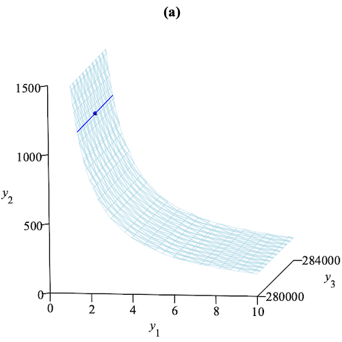
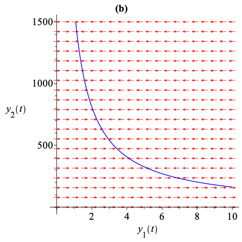
Figure 2: Critical manifolds and direction fields of our reductions of BioModel 716. (a) The surface is the critical manifold $\mathcal{M}_{\_}1^{*}\subseteq\mathcal{M}_{\_}0^{*}=\mathcal{U}$ projected from $\mathbb{R}^{4}$ into real $(y_{\_}1,y_{\_}2,y_{\_}3)$-space. The line located at $(y_{\_}1,y_{\_}2)\approx(1.4,1166.8)$ is the critical submanifold $\mathcal{M}_{\_}2^{*}\subseteq\mathcal{M}_{\_}1^{*}$. The dot located at $(y_{\_}1,y_{\_}2,y_{\_}3)\approx(1.4,1166.8,282049.2)$ is the critical submanifold $\mathcal{M}_{\_}3^{*}\subseteq\mathcal{M}_{\_}2^{*}$. Both $\mathcal{M}_{\_}1^{*}$ and $\mathcal{M}_{\_}2^{*}$ extend to $\pm\infty$ in both $y_{\_}3$ and $y_{\_}4$ direction, and $\mathcal{M}_{\_}3^{*}$ is located near $(1.4,1166.8,282049.2,1349.6)$. (b) The direction field of $T_{\_}1^{*}\circ R_{\_}1^{*}$ on $\mathcal{M}_{\_}0^{*}=\mathcal{U}$ projected from $\mathbb{R}^{4}$ into real $(y_{\_}1,y_{\_}2)$-space. The curve is the critical submanifold $\mathcal{M}_{\_}1^{*}\subseteq\mathcal{M}_{\_}0^{*}$. (c) The direction field of $T_{\_}2^{*}\circ R_{\_}2^{*}$ on $\mathcal{M}_{\_}1^{*}$ projected from $\mathbb{R}^{4}$ into real $(y_{\_}3,y_{\_}2)$-space. The line is the critical submanifold $\mathcal{M}_{\_}2^{*}\subseteq\mathcal{M}_{\_}1^{*}$. The system here is slower than the one in (b) by a factor of $125$. (d) The direction field of $T_{\_}3^{*}\circ R_{\_}3^{*}$ on $\mathcal{M}_{\_}2^{*}$ projected from $\mathbb{R}^{4}$ into real $(y_{\_}3,y_{\_}4)$-space. The dot is the critical submanifold $\mathcal{M}_{\_}3^{*}\subseteq\mathcal{M}_{\_}2^{*}$. The system here is slower than the one in (c) by another factor of $125$.

visualizes the direction fields of $T_{\_}1^{*}\circ R_{\_}1^{*}$, …, $T_{\_}3^{*}\circ R_{\_}3^{*}$ on their respective manifolds $\mathcal{M}_{\_}0^{*}$, …, $\mathcal{M}_{\_}2^{*}$ along with their respective critical manifolds $\mathcal{M}_{\_}1^{*}$, …, $\mathcal{M}_{\_}3^{*}$, where $\mathcal{M}_{\_}3^{*}$ can be derived from $\mathcal{M}_{\_}2^{*}$ by additionally equating the vector field of $T_{\_}3^{*}\circ R_{\_}3^{*}$ to zero:

$$\textstyle M_{\_}3^{*}=\bigl{[}y_{\_}1=\frac{4652377}{3335005},\quad y_{\_}2=\frac{5428474920}{4652377},\quad y_{\_}3=\frac{7051228977}{25000},\quad y_{\_}4=\frac{441466240042010928888}{327120760850763125}\bigr{]}.$$

This list $M_{\_}3^{*}$ does not explicitly occur in the output. However, its preimage $M_{\_}3$ is constructed in Algorithm 5 and justifies the presence of $(M_{\_}2,T_{\_}3,R_{\_}3)$ in the output there. The total computation time was 0.906 s.

This multiple-time scale reduction of the bird flu model emphasizes a cascade of successive relaxations of model variables. First, the population of susceptible birds relaxes. This relaxation is illustrated in Fig. 2(b). Then, the population of infected birds relaxes as shown in Fig. 2(c). Finally, the populations of susceptible and infected humans relax to a stable steady state as shown in Fig. 2(d), following a reduced dynamics described by $T_{\_}3^{*}$.

7.2 TGF-$\beta$ Pathway

BioModel 101 is a simple representation of the TGF-$\beta$ signaling pathway that plays a central role in tissue homeostasis and morphogenesis, as well as in numerous diseases such as fibrosis and cancer [76]. Concentrations over time of species Receptor 1 (RI), Receptor 2 (RII), Ligand receptor complex-plasma membrane (lRIRII), Ligand receptor complex-endosome (lRIRIIendo), Receptor 1 endosome (RIendo), and Receptor 2 endosome (RIIendo), are mapped to differential variables $y_{\_}1$, …, $y_{\_}6$, respectively. The original BioModel 101 has a change of ligand concentration at time $t=2500$. For our computation here, we ignore this discrete event. The input system is given by

$$S=\bigl{[}\textstyle{\frac{\operatorname{d}\!{}}{\operatorname{d}\!{t}}y_{\_}{1}} =\textstyle{-\frac{1}{100}y_{\_}{1}y_{\_}{2}-\frac{90277}{250000}y_{\_}{1}+\frac{33333}{1000000}y_{\_}{4}+\frac{33333}{1000000}y_{\_}{5}+8},$$

$$\textstyle{\frac{\operatorname{d}\!{}}{\operatorname{d}\!{t}}y_{\_}{2}} =\textstyle{-\frac{1}{100}y_{\_}{1}y_{\_}{2}-\frac{90277}{250000}y_{\_}{2}+\frac{33333}{1000000}y_{\_}{4}+\frac{33333}{1000000}y_{\_}{6}+4},$$

$$\textstyle{\frac{\operatorname{d}\!{}}{\operatorname{d}\!{t}}y_{\_}{3}} =\textstyle{\frac{1}{100}y_{\_}{1}y_{\_}{2}-\frac{152777}{250000}y_{\_}{3}},$$

$$\textstyle{\frac{\operatorname{d}\!{}}{\operatorname{d}\!{t}}y_{\_}{4}} =\textstyle{\frac{33333}{100000}y_{\_}{3}-\frac{33333}{1000000}y_{\_}{4}},$$

$$\textstyle{\frac{\operatorname{d}\!{}}{\operatorname{d}\!{t}}y_{\_}{5}} =\textstyle{\frac{33333}{100000}y_{\_}{1}-\frac{33333}{1000000}y_{\_}{5}},$$

$$\textstyle{\frac{\operatorname{d}\!{}}{\operatorname{d}\!{t}}y_{\_}{6}} =\textstyle{\frac{33333}{100000}y_{\_}{2}-\frac{33333}{1000000}y_{\_}{6}}\bigr{]}.$$

We choose $\varepsilon_{\_}*=\frac{1}{5}$, $p=1$, and select $D=(0,-4,-1,-2,-1,-5)$ from the tropical equilibrium. Our back-transformed reduced systems read as follows:

$$M_{\_}{0}^{*}=\bigl{[} \ \bigr{]}, T_{\_}{1}^{*}=\bigl{[} \textstyle{\frac{\operatorname{d}\!{}}{\operatorname{d}\!{t}}y_{\_}{1}}=\textstyle{5\cdot\left(-\frac{1}{500}y_{\_}{1}y_{\_}{2}+\frac{8}{5}\right)}\bigr{]},$$

$$R_{\_}{1}^{*}=\bigl{[} \textstyle{\frac{\operatorname{d}\!{}}{\operatorname{d}\!{t}}y_{\_}{2}}=0,\quad\textstyle{\frac{\operatorname{d}\!{}}{\operatorname{d}\!{t}}y_{\_}{3}}=0,\quad\textstyle{\frac{\operatorname{d}\!{}}{\operatorname{d}\!{t}}y_{\_}{4}}=0,\quad\textstyle{\frac{\operatorname{d}\!{}}{\operatorname{d}\!{t}}y_{\_}{5}}=0,$$

$$\textstyle{\frac{\operatorname{d}\!{}}{\operatorname{d}\!{t}}y_{\_}{6}}=0\bigr{]},$$

$$M_{\_}{1}^{*}=\bigl{[} \textstyle{y_{\_}{1}y_{\_}{2}}=\textstyle{800}\bigr{]}, T_{\_}{2}^{*}=\bigl{[} \textstyle{\frac{\operatorname{d}\!{}}{\operatorname{d}\!{t}}y_{\_}{3}}=\textstyle{1\cdot\left(-\frac{152777}{250000}y_{\_}{3}+8\right)}\bigr{]},$$

$$R_{\_}{2}^{*}=\bigl{[} \textstyle{\frac{\operatorname{d}\!{}}{\operatorname{d}\!{t}}y_{\_}{2}}=0,\quad\textstyle{\frac{\operatorname{d}\!{}}{\operatorname{d}\!{t}}y_{\_}{4}}=0,\quad\textstyle{\frac{\operatorname{d}\!{}}{\operatorname{d}\!{t}}y_{\_}{5}}=0,\quad\textstyle{\frac{\operatorname{d}\!{}}{\operatorname{d}\!{t}}y_{\_}{6}}=0\bigr{]},$$

$$M_{\_}{2}^{*}=\bigl{[} \textstyle{y_{\_}{1}y_{\_}{2}}=\textstyle{800}, T_{\_}{3}^{*}=\bigl{[} \textstyle{\frac{\operatorname{d}\!{}}{\operatorname{d}\!{t}}y_{\_}{2}}=\textstyle{\frac{1}{5}\cdot\left(-\frac{90277}{50000}y_{\_}{2}+\frac{33333}{200000}y_{\_}{6}\right)}\bigr{]},$$

$$\textstyle{y_{\_}{3}}=\textstyle{\frac{2000000}{152777}}\bigr{]}, R_{\_}{3}^{*}=\bigl{[} \textstyle{\frac{\operatorname{d}\!{}}{\operatorname{d}\!{t}}y_{\_}{4}}=0,\quad\textstyle{\frac{\operatorname{d}\!{}}{\operatorname{d}\!{t}}y_{\_}{5}}=0,\quad\textstyle{\frac{\operatorname{d}\!{}}{\operatorname{d}\!{t}}y_{\_}{6}}=0\bigr{]}.$$

The total computation time was 0.906 s.

The multiple-time scale reduction of the TGF-$\beta$ model emphasizes a cascade of successive relaxations of concentrations of different species. First, the concentration of receptor 1 relaxes rapidly. Then follows the membrane complex, and, even slower, the relaxation of receptor 2.

7.3 Caspase Activation Pathway

BioModel 102 is a quantitative kinetic model that examines the intrinsic pathway of caspase activation that is essential for apoptosis induction by various stimuli including cytotoxic stress [43]. Species concentrations over time are mapped to differential variables $y_{\_}1$, …, $y_{\_}{13}$ as described in Table 1.

Table 1: Mapping of species concentrations to differential variables for BioModel 102

Species	Species variable	Differential variable
APAF-1	A	$y_{\_}{1}$
Caspase 9	C9	$y_{\_}{2}$
Caspase 9-XIAP complex	C9X	$y_{\_}{3}$
XIAP	X	$y_{\_}{4}$
APAF-1-Caspase 9-XIAP complex	AC9X	$y_{\_}{5}$
APAF-1-Caspase 9 complex	AC9	$y_{\_}{6}$
Caspase 3	C3	$y_{\_}{7}$
Caspase 3 cleaved	C3star	$y_{\_}{8}$
Caspase 3 cleaved-XIAP complex	C3starX	$y_{\_}{9}$
Caspase 9 cleaved-XIAP complex	C9starX	$y_{\_}{10}$
Caspase 9 cleaved	C9star	$y_{\_}{11}$
APAF-1-Caspase 9 cleaved complex	AC9star	$y_{\_}{12}$
APAF-1-Caspase 9 cleaved-XIAP complex	AC9starX	$y_{\_}{13}$

The input system is given by

$$S=\bigl{[}\phantom{{}_{\_}3}\textstyle{\frac{\operatorname{d}\!{}}{\operatorname{d}\!{t}}y_{\_}{1}} =\textstyle{-\frac{1}{500}y_{\_}{1}y_{\_}{2}-\frac{1}{500}y_{\_}{1}y_{\_}{3}-\frac{1}{500}y_{\_}{1}y_{\_}{10}-\frac{1}{500}y_{\_}{1}y_{\_}{11}-\frac{1}{1000}y_{\_}{1}+\frac{1}{10}y_{\_}{5}+\frac{1}{10}y_{\_}{6}+\frac{1}{10}y_{\_}{12}}$$

$$\quad\quad\textstyle{{}+\frac{1}{10}y_{\_}{13}+\frac{1}{50}},$$

$$\textstyle{\frac{\operatorname{d}\!{}}{\operatorname{d}\!{t}}y_{\_}{2}} =\textstyle{-\frac{1}{500}y_{\_}{1}y_{\_}{2}-\frac{1}{1000}y_{\_}{2}y_{\_}{4}-\frac{1}{5000}y_{\_}{2}y_{\_}{8}-\frac{1}{1000}y_{\_}{2}+\frac{1}{1000}y_{\_}{3}+\frac{1}{10}y_{\_}{6}+\frac{1}{50}},$$

$$\textstyle{\frac{\operatorname{d}\!{}}{\operatorname{d}\!{t}}y_{\_}{3}} =\textstyle{-\frac{1}{500}y_{\_}{1}y_{\_}{3}+\frac{1}{1000}y_{\_}{2}y_{\_}{4}-\frac{1}{500}y_{\_}{3}+\frac{1}{10}y_{\_}{5}},$$

$$\textstyle{\frac{\operatorname{d}\!{}}{\operatorname{d}\!{t}}y_{\_}{4}} =\textstyle{-\frac{1}{1000}y_{\_}{2}y_{\_}{4}+\frac{1}{1000}y_{\_}{3}-\frac{1}{1000}y_{\_}{4}y_{\_}{6}-\frac{3}{1000}y_{\_}{4}y_{\_}{8}-\frac{1}{1000}y_{\_}{4}y_{\_}{11}-\frac{1}{1000}y_{\_}{4}y_{\_}{12}-\frac{1}{1000}y_{\_}{4}}$$

$$\quad\quad\textstyle{{}+\frac{1}{1000}y_{\_}{5}+\frac{1}{1000}y_{\_}{9}+\frac{1}{1000}y_{\_}{10}+\frac{1}{1000}y_{\_}{13}+\frac{1}{25}},$$

$$\textstyle{\frac{\operatorname{d}\!{}}{\operatorname{d}\!{t}}y_{\_}{5}} =\textstyle{\frac{1}{500}y_{\_}{1}y_{\_}{3}+\frac{1}{1000}y_{\_}{4}y_{\_}{6}-\frac{51}{500}y_{\_}{5}},$$

$$\textstyle{\frac{\operatorname{d}\!{}}{\operatorname{d}\!{t}}y_{\_}{6}} =\textstyle{\frac{1}{500}y_{\_}{1}y_{\_}{2}-\frac{1}{1000}y_{\_}{4}y_{\_}{6}+\frac{1}{1000}y_{\_}{5}-\frac{1}{5000}y_{\_}{6}y_{\_}{8}-\frac{101}{1000}y_{\_}{6}},$$

$$\textstyle{\frac{\operatorname{d}\!{}}{\operatorname{d}\!{t}}y_{\_}{7}} =\textstyle{-\frac{1}{200000}y_{\_}{2}y_{\_}{7}-\frac{7}{20000}y_{\_}{6}y_{\_}{7}-\frac{1}{20000}y_{\_}{7}y_{\_}{11}-\frac{7}{2000}y_{\_}{7}y_{\_}{12}-\frac{1}{1000}y_{\_}{7}+\frac{1}{5}},$$

$$\textstyle{\frac{\operatorname{d}\!{}}{\operatorname{d}\!{t}}y_{\_}{8}} =\textstyle{\frac{1}{200000}y_{\_}{2}y_{\_}{7}-\frac{3}{1000}y_{\_}{4}y_{\_}{8}+\frac{7}{20000}y_{\_}{6}y_{\_}{7}+\frac{1}{20000}y_{\_}{7}y_{\_}{11}+\frac{7}{2000}y_{\_}{7}y_{\_}{12}-\frac{1}{1000}y_{\_}{8}+\frac{1}{1000}y_{\_}{9}},$$

$$\textstyle{\frac{\operatorname{d}\!{}}{\operatorname{d}\!{t}}y_{\_}{9}} =\textstyle{\frac{3}{1000}y_{\_}{4}y_{\_}{8}-\frac{1}{500}y_{\_}{9}},$$

$$\textstyle{\frac{\operatorname{d}\!{}}{\operatorname{d}\!{t}}y_{\_}{10}} =\textstyle{-\frac{1}{500}y_{\_}{1}y_{\_}{10}+\frac{1}{1000}y_{\_}{4}y_{\_}{11}-\frac{1}{500}y_{\_}{10}+\frac{1}{10}y_{\_}{13}},$$

$$\textstyle{\frac{\operatorname{d}\!{}}{\operatorname{d}\!{t}}y_{\_}{11}} =\textstyle{-\frac{1}{500}y_{\_}{1}y_{\_}{11}+\frac{1}{5000}y_{\_}{2}y_{\_}{8}-\frac{1}{1000}y_{\_}{4}y_{\_}{11}+\frac{1}{1000}y_{\_}{10}-\frac{1}{1000}y_{\_}{11}+\frac{1}{10}y_{\_}{12}},$$

$$\textstyle{\frac{\operatorname{d}\!{}}{\operatorname{d}\!{t}}y_{\_}{12}} =\textstyle{\frac{1}{500}y_{\_}{1}y_{\_}{11}-\frac{1}{1000}y_{\_}{4}y_{\_}{12}+\frac{1}{5000}y_{\_}{6}y_{\_}{8}-\frac{101}{1000}y_{\_}{12}+\frac{1}{1000}y_{\_}{13}},$$

$$\textstyle{\frac{\operatorname{d}\!{}}{\operatorname{d}\!{t}}y_{\_}{13}} =\textstyle{\frac{1}{500}y_{\_}{1}y_{\_}{10}+\frac{1}{1000}y_{\_}{4}y_{\_}{12}-\frac{51}{500}y_{\_}{13}}\bigr{]}.$$

We choose $\varepsilon_{\_}*=\frac{1}{2}$, $p=1$, and select $D=(-4,2,3,5,5,4,-6,-8,-4,-2,-2,0,0)$ from the tropical equilibration. Our back-transformed reduced systems read as follows:

$$M_{\_}{0}^{*}=\bigl{[} \ \bigr{]}, T_{\_}{1}^{*}=\bigl{[} \textstyle{\frac{\operatorname{d}\!{}}{\operatorname{d}\!{t}}y_{\_}{4}}=\textstyle{1\cdot\left(-\frac{3}{1000}y_{\_}{4}y_{\_}{8}+\frac{1}{25}\right)}\bigr{]},$$

$$R_{\_}{1}^{*}=\bigl{[} \textstyle{\frac{\operatorname{d}\!{}}{\operatorname{d}\!{t}}y_{\_}{5}}=0,\quad\textstyle{\frac{\operatorname{d}\!{}}{\operatorname{d}\!{t}}y_{\_}{6}}=0,\quad\textstyle{\frac{\operatorname{d}\!{}}{\operatorname{d}\!{t}}y_{\_}{12}}=0,\quad\textstyle{\frac{\operatorname{d}\!{}}{\operatorname{d}\!{t}}y_{\_}{13}}=0,$$

$$\textstyle{\frac{\operatorname{d}\!{}}{\operatorname{d}\!{t}}y_{\_}{2}}=0,\quad\textstyle{\frac{\operatorname{d}\!{}}{\operatorname{d}\!{t}}y_{\_}{3}}=0,\quad\textstyle{\frac{\operatorname{d}\!{}}{\operatorname{d}\!{t}}y_{\_}{10}}=0,\quad\textstyle{\frac{\operatorname{d}\!{}}{\operatorname{d}\!{t}}y_{\_}{11}}=0,$$

$$\textstyle{\frac{\operatorname{d}\!{}}{\operatorname{d}\!{t}}y_{\_}{1}}=0,\quad\textstyle{\frac{\operatorname{d}\!{}}{\operatorname{d}\!{t}}y_{\_}{7}}=0,\quad\textstyle{\frac{\operatorname{d}\!{}}{\operatorname{d}\!{t}}y_{\_}{9}}=0,\quad\textstyle{\frac{\operatorname{d}\!{}}{\operatorname{d}\!{t}}y_{\_}{8}}=0\bigr{]},$$

$$M_{\_}{1}^{*}=\bigl{[} \textstyle{y_{\_}{4}y_{\_}{8}}=\textstyle{\frac{40}{3}}\bigr{]}, T_{\_}{2}^{*}=\bigl{[} \textstyle{\frac{\operatorname{d}\!{}}{\operatorname{d}\!{t}}y_{\_}{5}}=\textstyle{\frac{1}{8}\cdot\left(\frac{2}{125}y_{\_}{1}y_{\_}{3}-\frac{102}{125}y_{\_}{5}\right)},$$

$$\textstyle{\frac{\operatorname{d}\!{}}{\operatorname{d}\!{t}}y_{\_}{6}}=\textstyle{\frac{1}{8}\cdot\left(\frac{2}{125}y_{\_}{1}y_{\_}{2}-\frac{101}{125}y_{\_}{6}\right)},$$

$$\textstyle{\frac{\operatorname{d}\!{}}{\operatorname{d}\!{t}}y_{\_}{12}}=\textstyle{\frac{1}{8}\cdot\left(\frac{2}{125}y_{\_}{1}y_{\_}{11}-\frac{101}{125}y_{\_}{12}\right)},$$

$$\textstyle{\frac{\operatorname{d}\!{}}{\operatorname{d}\!{t}}y_{\_}{13}}=\textstyle{\frac{1}{8}\cdot\left(\frac{2}{125}y_{\_}{1}y_{\_}{10}-\frac{102}{125}y_{\_}{13}\right)}\bigr{]},$$

$$R_{\_}{2}^{*}=\bigl{[} \textstyle{\frac{\operatorname{d}\!{}}{\operatorname{d}\!{t}}y_{\_}{2}}=0,\quad\textstyle{\frac{\operatorname{d}\!{}}{\operatorname{d}\!{t}}y_{\_}{3}}=0,\quad\textstyle{\frac{\operatorname{d}\!{}}{\operatorname{d}\!{t}}y_{\_}{10}}=0,\quad\textstyle{\frac{\operatorname{d}\!{}}{\operatorname{d}\!{t}}y_{\_}{11}}=0,$$

$$\textstyle{\frac{\operatorname{d}\!{}}{\operatorname{d}\!{t}}y_{\_}{1}}=0,\quad\textstyle{\frac{\operatorname{d}\!{}}{\operatorname{d}\!{t}}y_{\_}{7}}=0,\quad\textstyle{\frac{\operatorname{d}\!{}}{\operatorname{d}\!{t}}y_{\_}{9}}=0,\quad\textstyle{\frac{\operatorname{d}\!{}}{\operatorname{d}\!{t}}y_{\_}{8}}=0\bigr{]},$$

$$M_{\_}{2}^{*}=\bigl{[} \textstyle{y_{\_}{4}y_{\_}{8}}=\textstyle{\frac{40}{3}}, T_{\_}{3}^{*}=\bigl{[} \textstyle{\frac{\operatorname{d}\!{}}{\operatorname{d}\!{t}}y_{\_}{2}}=\textstyle{\frac{1}{16}\cdot\left(-\frac{2}{625}y_{\_}{2}y_{\_}{8}+\frac{8}{25}\right)}\bigr{]},$$

$$\textstyle{y_{\_}{1}y_{\_}{3}-51y_{\_}{5}}=0, R_{\_}{3}^{*}=\bigl{[} \textstyle{\frac{\operatorname{d}\!{}}{\operatorname{d}\!{t}}y_{\_}{3}}=0,\quad\textstyle{\frac{\operatorname{d}\!{}}{\operatorname{d}\!{t}}y_{\_}{10}}=0,\quad\textstyle{\frac{\operatorname{d}\!{}}{\operatorname{d}\!{t}}y_{\_}{11}}=0,\quad\textstyle{\frac{\operatorname{d}\!{}}{\operatorname{d}\!{t}}y_{\_}{1}}=0,$$

$$\textstyle{2y_{\_}{1}y_{\_}{2}-101y_{\_}{6}}=0, \textstyle{\frac{\operatorname{d}\!{}}{\operatorname{d}\!{t}}y_{\_}{7}}=0,\quad\textstyle{\frac{\operatorname{d}\!{}}{\operatorname{d}\!{t}}y_{\_}{9}}=0,\quad\textstyle{\frac{\operatorname{d}\!{}}{\operatorname{d}\!{t}}y_{\_}{8}}=0\bigr{]}.$$

$$\textstyle{2y_{\_}{1}y_{\_}{11}-101y_{\_}{12}}=0,$$

$$\textstyle{y_{\_}{1}y_{\_}{10}-51y_{\_}{13}}=0\bigr{]},$$

The total computation time was 8.547 s, of which Algorithm 4 took 6.188 s.

The multiple-time scale reduction of the caspase activation model emphasizes a cascade of successive relaxations. First, the inhibitor of apoptosis XIAP binds rapidly to the cleaved caspase. Then, the four APAF complexes are formed. Finally, the Caspase 9 is recruited to the apoptosome.

7.4 Avian Influenza Bird-to-Human Transmission

BioModel 709 describes bird-to-human transmission of different strains of avian influenza A viruses, such as H5N1 and H7N9 [47]. Species concentrations over time of Susceptible avians (Sa), Infected avians (Ia), Susceptible humans (Sh), Infected humans (Ih), and Recovered humans (Rh) are mapped to differential variables $y_{\_}1$, …, $y_{\_}5$, respectively. The input system is given by

$$S=\bigl{[} \textstyle{\frac{\operatorname{d}\!{}}{\operatorname{d}\!{t}}y_{\_}{1}}=\textstyle{-\frac{1}{8000000000}y_{\_}{1}^{3}+\frac{127}{20000000}y_{\_}{1}^{2}-\frac{9}{500000000}y_{\_}{1}y_{\_}{2}-\frac{1}{200}y_{\_}{1}},$$

$$\textstyle{\frac{\operatorname{d}\!{}}{\operatorname{d}\!{t}}y_{\_}{2}}=\textstyle{\frac{9}{500000000}y_{\_}{1}y_{\_}{2}-\frac{37123}{50000000}y_{\_}{2}},$$

$$\textstyle{\frac{\operatorname{d}\!{}}{\operatorname{d}\!{t}}y_{\_}{3}}=\textstyle{-\frac{3}{500000000}y_{\_}{2}y_{\_}{3}-\frac{391}{10000000}y_{\_}{3}+30},$$

$$\textstyle{\frac{\operatorname{d}\!{}}{\operatorname{d}\!{t}}y_{\_}{4}}=\textstyle{\frac{3}{500000000}y_{\_}{2}y_{\_}{3}-\frac{4445391}{10000000}y_{\_}{4}},$$

$$\textstyle{\frac{\operatorname{d}\!{}}{\operatorname{d}\!{t}}y_{\_}{5}}=\textstyle{\frac{1}{10}y_{\_}{4}-\frac{391}{10000000}y_{\_}{5}}\bigr{]}.$$

We choose $\varepsilon_{\_}*=\frac{1}{5}$, $p=1$, and select $D=(-7,0,-8,3,-2)$ from the tropical equilibration. Our back-transformed reduced systems read as follows:

$$M^{*}_{\_}{0} =\bigl{[}\ \bigr{]}, T^{*}_{\_}{1}=\bigl{[} \textstyle{\frac{\operatorname{d}\!{}}{\operatorname{d}\!{t}}y_{\_}{1}}=1\cdot\left(\textstyle{-\frac{1}{8000000000}y_{\_}{1}^{3}+\frac{127}{20000000}y_{\_}{1}^{2}}\right)\bigr{]},$$

$$R_{\_}{1}^{*}=\bigl{[} \textstyle{\frac{\operatorname{d}\!{}}{\operatorname{d}\!{t}}y_{\_}{4}}=0,\quad\textstyle{\frac{\operatorname{d}\!{}}{\operatorname{d}\!{t}}y_{\_}{2}}=0,\quad\textstyle{\frac{\operatorname{d}\!{}}{\operatorname{d}\!{t}}y_{\_}{3}}=0,\quad\textstyle{\frac{\operatorname{d}\!{}}{\operatorname{d}\!{t}}y_{\_}{5}}=0\bigr{]},$$

$$M^{*}_{\_}{1} =\bigl{[}\textstyle{y_{\_}{1}^{3}-50800y_{\_}{1}^{2}}=0\bigr{]}, T^{*}_{\_}{2}=\bigl{[} \textstyle{\frac{\operatorname{d}\!{}}{\operatorname{d}\!{t}}y_{\_}{4}}=\textstyle{\frac{1}{5}\cdot\left(\frac{3}{100000000}y_{\_}{2}y_{\_}{3}-\frac{4445391}{2000000}y_{\_}{4}\right)}\bigr{]},$$

$$R_{\_}{2}^{*}=\bigl{[} \textstyle{\frac{\operatorname{d}\!{}}{\operatorname{d}\!{t}}y_{\_}{2}}=0,\quad\textstyle{\frac{\operatorname{d}\!{}}{\operatorname{d}\!{t}}y_{\_}{3}}=0,\quad\textstyle{\frac{\operatorname{d}\!{}}{\operatorname{d}\!{t}}y_{\_}{5}}=0\bigr{]}.$$

The total computation time was 0.578 s.

The multiple-time scale reduction of this avian influenza model emphasizes a cascade of successive relaxations of different model variables. First, the susceptible bird population relaxes rapidly. The reduced equation $T_{\_}1$ and manifold $M_{\_}1$ suggest that the bird population dynamics is of the Allee type and evolves toward the stable extinct state. It follows the relaxation of infected human population that also evolves toward the extinct state, the end of the epidemics.

8 Some Remarks on Complexity

A detailed complexity analysis of our approach is beyond the scope of this article. We collect some remarks on the asymptotic worst-case complexity of various computational steps required by our algorithms:

1. the existential decision problem over real closed fields, for which we use SMT solving over QF_NRA in Algorithm 6;

2. linear programming, for which we used SMT solving over QF_LRA in Algorithm 3;

3. integer linear programming, for which we used SMT solving over QF_LIA in Algorithm 7.

Problem (i) is in single exponential time [32]. Problem (ii) is in polynomial [38] time. Problem (iii) is NP-complete; a proof can be found in [65, Theorem 18.1], where it is essentially attributed to [16]. With all these problems, the dominant complexity parameter is the number of variables, which in our context corresponds to the number $n$ of differential variables. Biological models impose reasonable upper bounds on $n$, which corresponds to the number of species occurring there. When $n$ is bounded, problem (i) becomes polynomial [32]. The same holds for problem (iii); a proof based on Lenstra’s algorithm [44] can be found in [65, Corollary 18.7a].

When characterizing the decision in l.2 of Algorithm 3 as linear programming in (ii) above, we tacitly assume that it is not applied to the tropical equilibration $\Pi$ as a whole but to each contained polyhedron independently. The number of contained polyhedra is in turn exponential in $n$, in the worst case. The motivation for the computation of a disjunctive normal form in Algorithm 4 is to support the choice of a suitable point $(d_{\_}1,\dots,d_{\_}n)$ in Algorithm 3 by providing information on the geometry of the tropical equilibration as a union of polyhedra. It is possible to omit this and accordingly drop the computation of the disjunctive normal form in l.23 of Algorithm 4 altogether. In that case, solving in l.2 of Algorithm 3 is applied to the formula $\bigwedge\bigvee\bigwedge P$ instead of $\Pi$. This is a linear decision problem over ordered fields, which is NP-complete [29], and solutions can be found in single exponential time [79].

Efficient implementations do not necessarily use theoretically optimal algorithms. At the time of writing, SMT solving and corresponding decision procedures are a very active field of research and thus subject to constant change. We deliberately refrain from going into details about the current state of the art at this point.

Beyond the examples and computation times discussed here, we currently have no systematic empirical data that would allow substantial statements on the practical performance and limits of our implementations.

9 Concluding Remarks

We provided a symbolic method for automated model reduction of biological networks described by ordinary differential equations with multiple time scales. Our method is applicable to systems with two time scales or more, superseding traditional slow-fast reduction methods that can cope withonly two time scales. We also proposed, for the first time, the automatic verification of hyperbolicity conditions required for the validity of the reduction. Our theoretical framework is accompanied by rigorous algorithms and prototypical implementations, which we successfully applied to real-world problems from the BioModels database [57].

We would like to list some open points and possible extensions of our research here. Our reduction algorithm is based on a fixed scaling (8) leading to a fixed ordering of the time scales of different variables. In our reduction scheme, different variables relax hierarchically, first the fastest ones, then the second fastest, and finally the slowest ones, which justifies our geometric picture of nested invariant manifolds. However, there are situations, e.g. in models of relaxation oscillations, when the ordering of time scales changes with time: variables that were fast can become slow at a later time, and vice versa. In order to cope with such situations, one would like to use different scalings for different time segments. One attempt to implement such a procedure has been provided in [68].

Although our proposed method identifies the full hierarchy of time scales, the subsequent reduction may stop early in this hierarchy when hyperbolic attractivity is not satisfied at some stage. One possible reason is the presence of conservation laws, also known as first integrals, at the given reduction stage. Such conservation laws force an eigenvalue zero for the Jacobian. A theorem by Schneider and Wilhelm [64] can be employed to reduce such a setting to the hyperbolically attractive case. As for the behavior of first integrals when proceeding to the reduced system, see the discussion of the non-standard case in [41] for two time scales; an extension to multiple time scales should be straightforward. Work in progress is concerned with the introduction of new slow variables, one for each independent conservation law of the fast subsystem. This is applied to networks with multiple time scales and approximate linear and polynomial conservation laws.

More generally, it is of interest to consider cases when hyperbolic attractivity fails but hyperbolicity still holds: In such cases, Cardin and Teixeira show there still exist invariant manifolds [11]. Testing for hyperbolicity is more involved than testing for hyperbolic attractivity, but in theory it is well understood, and there exists an algorithmic approach due to Routh [27]. In the case of hyperbolicity, but not attractivity, the ensuing global dynamics may be quite interesting; for instance slow-fast cycles may appear.

Concerning differentiability requirements, we check in Sect. 3.3 for smoothness of the full system. However, Fenichel’s results, and in principle also those by Cardin and Teixeira, require only sufficient finite differentiability. Therefore, given a differential equation system and a scaling, invariant manifolds and corresponding reduced systems exist for $C^{p}$ functions with fixed $p<\infty$. Going through the details will involve intricate analysis that is left to future work.

In the introduction we sketched a Michaelis–Menten system abstracting from the known numerical values for the reaction rate constants $k_{\_}1$, $k_{\_}{-1}$, $k_{\_}2$. It would be indeed interesting to work on such parametric data. In the presence of parameters, one would consider effective quantifier elimination over real closed fields [15, 80, 20, 39, 69, 70] as a generalization of SMT solving. Robust implementations are freely available [9, 19] and well supported. They have been successfully applied to problems in chemical reaction network theory during the past decade [71, 72, 78, 23, 22, 7, 21, 8, 33, 67]. Such a generalization is not quite straightforward. With the tropical scaling in Sect. 2.2, Algorithm 2 would introduce logarithms of polynomials in the parametric coefficients, which is not compatible with the logic framework used here. Similar tropicalization methods, which are unfortunately not compatible with our abstract view on scaling in Sect. 2.1, require only logarithms of individual parametric coefficients [63]. Such a more special form would allow the use of abstraction in the logic engine.

From a point of view of user-oriented software, it would be most desirable to develop automatic strategies for determining good values for $\varepsilon_{\_}*$ and for choices of $(d_{\_}1,\dots,d_{\_}n)$ from the tropical equilibration in Algorithm 3.

Appendix A Further Computational Examples

Recall that in Sect. 7 we have discussed computations for several systems from the BioModels database [57]. While the focus there was on biological results, we discuss here examples where reduction stops at $\ell<m$ for various reasons. Again, we have conducted our computations on a standard desktop computer with a 3.3 GHz 6-core Intel 5820K CPU and 16 GB of main memory. Computation times listed are CPU times.

A.1 Hypertoxiticy of a Painkiller

BioModel 609 describes the metabolism and the related hepatotoxicity of acetaminophen, a pain killer [60]. The species concentrations over time of Sulphate PAPS, GSH, NAPQI, Paracetamol APAP, and Protein adducts are mapped to differential variables $y_{\_}1$, …, $y_{\_}5$, respectively. The input system is given by

$$S=\bigl{[} \textstyle{\frac{\operatorname{d}\!{}}{\operatorname{d}\!{t}}y_{\_}{1}}=\textstyle{-226000000000000y_{\_}{1}y_{\_}{4}-2y_{\_}{1}+\frac{53}{2000000000000000}},$$

$$\textstyle{\frac{\operatorname{d}\!{}}{\operatorname{d}\!{t}}y_{\_}{2}}=\textstyle{-1600000000000000000y_{\_}{2}y_{\_}{3}-2y_{\_}{2}+\frac{687}{50000000000000000}},$$

$$\textstyle{\frac{\operatorname{d}\!{}}{\operatorname{d}\!{t}}y_{\_}{3}}=\textstyle{-1600000000000000000y_{\_}{2}y_{\_}{3}-\frac{220063}{2000}y_{\_}{3}+\frac{63}{200}y_{\_}{4}},$$

$$\textstyle{\frac{\operatorname{d}\!{}}{\operatorname{d}\!{t}}y_{\_}{4}}=\textstyle{-226000000000000y_{\_}{1}y_{\_}{4}+\frac{63}{2000}y_{\_}{3}-\frac{661}{200}y_{\_}{4}},$$

$$\textstyle{\frac{\operatorname{d}\!{}}{\operatorname{d}\!{t}}y_{\_}{5}}=\textstyle{110y_{\_}{3}}\bigr{]}.$$

Since there is only one monomial on the right hand side of the equation for $\frac{\operatorname{d}\!{}}{\operatorname{d}\!{t}}y_{\_}5$, equilibration is impossible. This causes Algorithm 4 to return in l.23 a disjunctive normal form $\Pi$ equivalent to “false,” which describes the empty set. Hence Algorithm 3 returns $\bot$, and Algorithm 1 returns the empty list. The total computation time was 0.006 s.

A.2 Transmission Dynamics of Rabies

BioModel 726 examines the transmission dynamics of rabies between dogs and humans [61]. Species concentrations over time are mapped to differential variables $y_{\_}1$, …, $y_{\_}{8}$ as described in Table 2.

Table 2: Mapping of species concentrations to differential variables for BioModel 726

Species	Species variable	Differential variable
Susceptible dogs	Sd	$y_{\_}1$
Exposed dogs	Ed	$y_{\_}2$
Infectious dogs	Id	$y_{\_}3$
Recovered dogs	Rd	$y_{\_}4$
Susceptible humans	Sh	$y_{\_}5$
Exposed humans	Eh	$y_{\_}6$
Infectious humans	Ih	$y_{\_}7$
Recovered humans	Rh	$y_{\_}8$

The input system is given by

$$S=\bigl{[} \textstyle{\frac{\operatorname{d}\!{}}{\operatorname{d}\!{t}}y_{\_}{1}}=\textstyle{-\frac{79}{500000000}y_{\_}{1}y_{\_}{3}-\frac{17}{100}y_{\_}{1}+\frac{18}{5}y_{\_}{2}+y_{\_}{4}+3000000},$$

$$\textstyle{\frac{\operatorname{d}\!{}}{\operatorname{d}\!{t}}y_{\_}{2}}=\textstyle{\frac{79}{500000000}y_{\_}{1}y_{\_}{3}-\frac{617}{100}y_{\_}{2}},$$

$$\textstyle{\frac{\operatorname{d}\!{}}{\operatorname{d}\!{t}}y_{\_}{3}}=\textstyle{\frac{12}{5}y_{\_}{2}-\frac{27}{25}y_{\_}{3}},$$

$$\textstyle{\frac{\operatorname{d}\!{}}{\operatorname{d}\!{t}}y_{\_}{4}}=\textstyle{\frac{9}{100}y_{\_}{1}+\frac{9}{100}y_{\_}{2}-\frac{27}{25}y_{\_}{4}},$$

$$\textstyle{\frac{\operatorname{d}\!{}}{\operatorname{d}\!{t}}y_{\_}{5}}=\textstyle{-\frac{229}{100000000000000}y_{\_}{3}y_{\_}{5}-\frac{3}{1000}y_{\_}{5}+\frac{18}{5}y_{\_}{6}+y_{\_}{8}+15400000},$$

$$\textstyle{\frac{\operatorname{d}\!{}}{\operatorname{d}\!{t}}y_{\_}{6}}=\textstyle{\frac{229}{100000000000000}y_{\_}{3}y_{\_}{5}-\frac{6543}{1000}y_{\_}{6}},$$

$$\textstyle{\frac{\operatorname{d}\!{}}{\operatorname{d}\!{t}}y_{\_}{7}}=\textstyle{\frac{12}{5}y_{\_}{6}-\frac{1343}{1000}y_{\_}{7}},$$

$$\textstyle{\frac{\operatorname{d}\!{}}{\operatorname{d}\!{t}}y_{\_}{8}}=\textstyle{\frac{27}{50}y_{\_}{6}-\frac{1003}{1000}y_{\_}{8}}\bigr{]}.$$

We choose $\varepsilon_{\_}*=\frac{1}{5}$, $p=1$, and Algorithm 3 selects $D=(-10,-10,-11,-9,-14,-7,-8,-7)$ from the tropical equilibration. Algorithm 1 then yields the following scaled and truncated system with three time scales:

$$T_{\_}{1}=\bigl{[}\textstyle{\frac{\operatorname{d}\!{}}{\operatorname{d}\!{\tau}}x_{\_}{1}} =\textstyle{1\cdot\left(-\frac{395}{256}x_{\_}{1}x_{\_}{3}+\frac{18}{25}x_{\_}2\right)},$$

$$\textstyle{\frac{\operatorname{d}\!{}}{\operatorname{d}\!{\tau}}x_{\_}{2}} =\textstyle{1\cdot\left(\frac{395}{256}x_{\_}{1}x_{\_}{3}-\frac{617}{500}x_{\_}2\right)},$$

$$\textstyle{\frac{\operatorname{d}\!{}}{\operatorname{d}\!{\tau}}x_{\_}{6}} =\textstyle{1\cdot\left(\frac{28625}{16384}x_{\_}{3}x_{\_}{5}-\frac{6543}{5000}x_{\_}6\right)}\bigr{]},$$

$$T_{\_}{2}=\bigl{[}\textstyle{\frac{\operatorname{d}\!{}}{\operatorname{d}\!{\tau}}x_{\_}{3}} =\textstyle{\delta\cdot\left(\frac{12}{25}x_{\_}{2}-\frac{27}{25}x_{\_}{3}\right)},$$

$$\textstyle{\frac{\operatorname{d}\!{}}{\operatorname{d}\!{\tau}}x_{\_}{4}} =\textstyle{\delta\cdot\left(\frac{9}{20}x_{\_}{1}+\frac{9}{20}x_{\_}{2}-\frac{27}{25}x_{\_}{4}\right)},$$

$$\textstyle{\frac{\operatorname{d}\!{}}{\operatorname{d}\!{\tau}}x_{\_}{7}} =\textstyle{\delta\cdot\left(\frac{12}{25}x_{\_}{6}-\frac{1343}{1000}x_{\_}{7}\right)},$$

$$\textstyle{\frac{\operatorname{d}\!{}}{\operatorname{d}\!{\tau}}x_{\_}{8}} =\textstyle{\delta\cdot\left(\frac{27}{50}x_{\_}{6}-\frac{1003}{1000}x_{\_}{8}\right)}\bigr{]},$$

$$T_{\_}{3}=\bigl{[}\textstyle{\frac{\operatorname{d}\!{}}{\operatorname{d}\!{\tau}}x_{\_}{5}} =\textstyle{\delta^{5}\cdot\left(\frac{4928}{3125}-\frac{15}{8}x_{\_}{5}\right)}\bigr{]}.$$

Equating the right hand sides $F_{\_}1$ of the differential equations in $T_{\_}1$ to zero equivalently yields

$$M_{\_}1=[-9875x_{\_}{1}x_{\_}{3}+4608x_{\_}{2}=0,\quad 49375x_{\_}{1}x_{\_}{3}-39488x_{\_}{2}=0,\quad 17890625x_{\_}{3}x_{\_}{5}-13400064x_{\_}{6}=0].$$

In l.1 of Algorithm 6, $U\circ M_{\_}1$ is tested for satisfiability. This fails, which means that the corresponding manifold $\mathcal{M}_{\_}1$ is empty over the positive first orthant. Consequently, Algorithms 5, 8, and 9 return empty lists. The total computation time was 0.921 s.

A.3 Negative Feedback Loop Between Tumor Suppressor and Oncogene

BioModel 156 describes the dynamics of a negative feedback loop between the tumor suppressor protein p53 and the oncogene protein Mdm2 in human cells [30]. The species concentrations over time for P53 (x), Mdm2 (y), and Precursor Mdm2 (y0) are mapped to differential variables $y_{\_}1$, …, $y_{\_}3$, respectively. The input system is given by

$$S=\bigl{[} \textstyle{\frac{\operatorname{d}\!{}}{\operatorname{d}\!{t}}y_{\_}{1}}=\textstyle{-\frac{37}{10}y_{\_}{1}y_{\_}{2}+2y_{\_}{1}},$$

$$\textstyle{\frac{\operatorname{d}\!{}}{\operatorname{d}\!{t}}y_{\_}{2}}=\textstyle{-\frac{9}{10}y_{\_}{2}+\frac{11}{10}y_{\_}{3}},$$

$$\textstyle{\frac{\operatorname{d}\!{}}{\operatorname{d}\!{t}}y_{\_}{3}}=\textstyle{\frac{3}{2}y_{\_}{1}-\frac{11}{10}y_{\_}{3}}\bigr{]}.$$

We choose $\varepsilon_{\_}*=\frac{1}{2}$, $p=1$, and select $D=(2,1,1)$. Algorithm 1 then yields the following scaled and truncated system with two time scales:

$$T_{\_}{1}=\bigl{[}\textstyle{\frac{\operatorname{d}\!{}}{\operatorname{d}\!{\tau}}x_{\_}{1}} =\textstyle{1\cdot\left(-\frac{37}{40}x_{\_}{1}x_{\_}{2}+x_{\_}1\right)}\bigr{]},$$

$$T_{\_}{2}=\bigl{[}\textstyle{\frac{\operatorname{d}\!{}}{\operatorname{d}\!{\tau}}x_{\_}{2}} =\textstyle{\delta\cdot\left(-\frac{9}{10}x_{\_}{2}+\frac{11}{10}x_{\_}{3}\right)},$$

$$\textstyle{\frac{\operatorname{d}\!{}}{\operatorname{d}\!{\tau}}x_{\_}{3}} =\textstyle{\delta\cdot\left(\frac{3}{4}x_{\_}{1}-\frac{11}{10}x_{\_}{3}\right)}\bigr{]}.$$

Analogously to the previous section we obtain $M_{\_}1=[-37x_{\_}{1}x_{\_}{2}+40x_{\_}{1}=0]$, for which we find $\mathcal{M}_{\_}1$ to be non-empty over the positive first orthant in l.1 of Algorithm 6. However in l.20, the test for hyperbolic attractivity fails with $M_{\_}1$ and the Hurwitz conditions

$$\textstyle\Gamma=\left\{\frac{37}{40}x_{\_}2-1>0\right\},$$

so that “false” is returned. Therefore, Algorithm 5 breaks the for-loop in l.10 with $k=1$ and returns the empty list in l.19. Obviously, the simplified and back-translated systems are empty lists as well. The total computation time was 0.453 s.

A.4 CD4 T-Cells in the Spread of HIV

BioModel 663 describes how CD4 T-cells can influence the spread of the HIV infection [81]. Species concentrations over time for Infected T-cells (x), Uninfected T-cells (y), and Free viruses (v) are mapped to variables $y_{\_}1$, …, $y_{\_}3$, respectively. The input system is given by

$$S=\bigl{[} \textstyle{\frac{\operatorname{d}\!{}}{\operatorname{d}\!{t}}y_{\_}{1}}=\textstyle{-\frac{1}{10}y_{\_}{1}^{2}y_{\_}{3}-\frac{1}{10}y_{\_}{1}y_{\_}{2}y_{\_}{3}+\frac{4}{5}y_{\_}{1}y_{\_}{3}-\frac{1}{10}y_{\_}{1}},$$

$$\textstyle{\frac{\operatorname{d}\!{}}{\operatorname{d}\!{t}}y_{\_}{2}}=\textstyle{-\frac{1}{10}y_{\_}{1}y_{\_}{2}y_{\_}{3}+\frac{1}{5}y_{\_}{1}y_{\_}{3}-\frac{1}{10}y_{\_}{2}^{2}y_{\_}{3}+y_{\_}{2}y_{\_}{3}-\frac{1}{5}y_{\_}{2}},$$

$$\textstyle{\frac{\operatorname{d}\!{}}{\operatorname{d}\!{t}}y_{\_}{3}}=\textstyle{y_{\_}{2}-\frac{1}{2}y_{\_}{3}}\bigr{]}.$$

We choose $\varepsilon_{\_}*=\frac{1}{2}$, $p=5$, and $D=(1,4,3)$. The choice of $p=5$ causes fractional powers of numbers in the scaled and truncated system

$$\textstyle T_{\_}{1} =\textstyle\left[\frac{\operatorname{d}\!{}}{\operatorname{d}\!{\tau}}x_{\_}{3}=1\cdot\left(x_{\_}{2}-x_{\_}{3}\right)\right],$$

$$\textstyle T_{\_}{2} =\textstyle\left[\frac{\operatorname{d}\!{}}{\operatorname{d}\!{\tau}}x_{\_}{2}=\delta^{7}\cdot\left(\frac{4}{5}\sqrt[5]{4}\,x_{\_}{1}x_{\_}{3}-\frac{4}{5}\sqrt[5]{4}\,x_{\_}{2}\right)\right],$$

$$\textstyle T_{\_}{3} =\textstyle\left[\frac{\operatorname{d}\!{}}{\operatorname{d}\!{\tau}}x_{\_}{1}=\delta^{12}\cdot\left(\frac{4}{5}\sqrt[5]{4}\,x_{\_}{1}x_{\_}{3}-\frac{4}{5}\sqrt[5]{4}\,x_{\_}{1}\right)\right].$$

However, such input is not accepted with the SMT logic QF_NRA used in Algorithm 6. As discussed in Sect. 3.2, we catch the corresponding error from the SMT solver, convert to floats, and restart, which solves the problem.

Similarly to the previous example, the Hurwitz test in l.20 of Algorithm 6 succeeds for $k=1$ but fails for $k=2$ in Algorithm 5. Since there are fewer than two reduced systems, we return the empty list. Consequently, the list of simplified reduced systems and the corresponding list of back-transformed systems are empty as well. The total computation time was 0.390 s.

References

- [1] Clark Barrett, Christopher L. Conway, Morgan Deters, Liana Hadarean, Dejan Jovanović, Tim King, Andrew Reynolds, and Cesare Tinelli. CVC4. In G. Gopalakrishnan and S. Qadeer, editors, Proc. CAV 2011, volume 6806 of LNCS, pages 171–177. Springer, 2011. doi:10.1007/978-3-642-22110-1_14.
- [2] Clark Barrett, Pascal Fontaine, and Cesare Tinelli. The SMT-LIB standard: Version 2.6. Technical report, Department of Computer Science, The University of Iowa, 2017.
- [3] Thomas Becker, Volker Weispfenning, and Heinz Kredel. Gröbner Bases, a Computational Approach to Commutative Algebra, volume 141 of Graduate Texts in Mathematics. Springer, 1993. doi:10.1007/978-1-4612-0913-3.
- [4] Tristram Bogart, Anders Nedergaard Jensen, David Speyer, Bernd Sturmfels, and Rekha R. Thomas. Computing tropical varieties. J. Symb. Comput., 42(1–2):54–73, January–February 2007. doi:10.1016/j.jsc.2006.02.004.
- [5] François Boulier, François Fages, Ovidiu Radulescu, Satya S. Samal, Aandreas Schuppert, Werner M. Seiler, Thomas Sturm, Sebastian Walcher, and Anderas Weber. The SYMBIONT project: Symbolic methods for biological networks. F1000Research, 7(1341), August 2018. doi:10.7490/f1000research.1115995.1.
- [6] François Boulier, François Fages, Ovidiu Radulescu, Satya S. Samal, Andreas Schuppert, Werner M. Seiler, Thomas Sturm, Sebastian Walcher, and Andreas Weber. The SYMBIONT project: Symbolic methods for biological networks. ACM Communications in Computer Algebra, 52(3):67–70, December 2018. doi:10.1145/3313880.3313885.
- [7] Russell Bradford, James H. Davenport, Matthew England, Hassan Errami, Vladimir Gerdt, Dima Grigoriev, Charles Hoyt, Marek Košta, Ovidiu Radulescu, Thomas Sturm, and Andreas Weber. A case study on the parametric occurrence of multiple steady states. In M. Burr, editor, Proc. ISSAC 2017, pages 45–52. ACM, 2017. doi:10.1145/3087604.3087622.
- [8] Russell Bradford, James H. Davenport, Matthew England, Hassan Errami, Vladimir Gerdt, Dima Grigoriev, Charles Hoyt, Marek Košta, Ovidiu Radulescu, Thomas Sturm, and Andreas Weber. Identifying the parametric occurrence of multiple steady states for some biological networks. J. Symb. Comput., 98:84–119, May–June 2020. doi:10.1016/j.jsc.2019.07.008.
- [9] Christopher W. Brown. QEPCAD B: A program for computing with semi-algebraic sets using CADs. ACM SIGSAM Bulletin, 37(4):97–108, December 2003. doi:10.1145/968708.968710.
- [10] Bruno Buchberger. Ein Algorithmus zum Auffinden der Basiselemente des Restklassenringes nach einem nulldimensionalen Polynomideal. Doctoral dissertation, Mathematical Institute, University of Innsbruck, Innsbruck, Austria, 1965.
- [11] Pedro T. Cardin and Marco A. Teixeira. Fenichel theory for multiple time scale singular perturbation problems. SIAM J. Appl. Dyn. Syst., 16(3):1425–1452, January 2017. doi:10.1137/16m1067202.
- [12] Pedro T. Cardin and Marco A. Teixeira. Corrigendum: Fenichel theory for multiple time scale singular perturbation problems. SIAM J. Appl. Dyn. Syst., 18(2):1223, January 2019. doi:10.1137/19M1241660.
- [13] Alessandro Cimatti, Alberto Griggio, Bastiaan Schaafsma, and Roberto Sebastiani. The MathSAT5 SMT solver. In N. Piterman and S. A. Smolka, editors, Proc. TACAS 2013, volume 7795 of LNCS, pages 93–107. Springer, 2013. doi:10.1007/978-3-642-36742-7_7.
- [14] George E. Collins. Quantifier elimination for the elementary theory of real closed fields by cylindrical algebraic decomposition. In H. Brakhage, editor, Automata Theory and Formal Languages. 2nd GI Conference, volume 33 of LNCS, pages 134–183. Springer, 1975. doi:10.1007/3-540-07407-4_17.
- [15] George E. Collins and Hoon Hong. Partial cylindrical algebraic decomposition for quantifier elimination. J. Symb. Comput., 12(3):299–328, September 1991. doi:10.1016/S0747-7171(08)80152-6.
- [16] Stephen A. Cook. The complexity of theorem-proving procedures. In Proc. STOC ’71, pages 151–158. ACM Press, New York, NY, 1971. doi:10.1145/800157.805047.
- [17] Florian Corzilius, Gereon Kremer, Sebastian Junges, Stefan Schupp, and Erika Ábrahám. SMT-RAT: An open source C++ toolbox for strategic and parallel SMT solving. In M. Heule and S. Weaver, editors, Proc. SAT 2015, volume 9340 of LNCS, pages 360–368. Springer, 2015. doi:10.1007/978-3-319-24318-4_26.
- [18] Haskell B. Curry and Robert Feys. Combinatory Logic, volume I of Studies in Logic and the Foundations of Mathematics. North Holland Publishing Company, Amsterdam, The Netherlands, 1958.
- [19] Andreas Dolzmann and Thomas Sturm. Redlog: Computer algebra meets computer logic. ACM SIGSAM Bulletin, 31(2):2–9, June 1997. doi:10.1145/261320.261324.
- [20] Andreas Dolzmann, Thomas Sturm, and Volker Weispfenning. Real quantifier elimination in practice. In B. H. Matzat, G.-M. Greuel, and G. Hiss, editors, Algorithmic Algebra and Number Theory, pages 221–247. Springer, 1998. doi:10.1007/978-3-642-59932-3_11.
- [21] Matthew England, Hassan Errami, Dima Grigoriev, Ovidiu Radulescu, Thomas Sturm, and Andreas Weber. Symbolic versus numerical computation and visualization of parameter regions for multistationarity of biological networks. In Proc. CASC 2017, volume 10490 of LNCS, pages 93–108. Springer, 2017. doi:10.1007/978-3-319-66320-3_8.
- [22] Hassan Errami, Markus Eiswirth, Dima Grigoriev, Werner M. Seiler, Thomas Sturm, and Andreas Weber. Detection of Hopf bifurcations in chemical reaction networks using convex coordinates. J. Comput. Phys., 291:279–302, June 2015. doi:10.1016/j.jcp.2015.02.050.
- [23] Hassan Errami, Werner M. Seiler, Thomas Sturm, and Andreas Weber. On Muldowney’s criteria for polynomial vector fields with constraintsja. In V. P. Gerdt, W. Koepf, E. W. Mayr, and E. V. Vorozhtsov, editors, Proc. CASC 2011, volume 6885 of LNCS, pages 135–143. Springer, 2011. doi:10.1007/978-3-642-23568-9_11.
- [24] Martin Feinberg. Foundations of Chemical Reaction Network Theory, volume 202 of Applied Mathematical Sciences. Springer, 2019. doi:10.1007/978-3-030-03858-8.
- [25] Neil Fenichel. Geometric singular perturbation theory for ordinary differential equations. J. Differ. Equations, 31(1):53–98, January 1979. doi:10.1016/0022-0396(79)90152-9.
- [26] Stephen Forrest. Integration of SMT-LIB support into Maple. In M. England and V. Ganesch, editors, Proc. Satisfiability Checking and Symbolic Computation 2017, volume 1974 of CEUR Workshop Proceedings. CEUR-WS, Kaiserslautern, Germany, July 2017. doi:10.1145/3055282.3055285.
- [27] Feliks R. Gantmacher. The Theory of Matrices. Vol. 2. Transl. from the Russian by K. A. Hirsch. Providence, RI: AMS Chelsea Publishing, reprint of the 1959 translation edition, 1998.
- [28] Marco Gario and Andrea Micheli. PySMT: A solver-agnostic library for fast prototyping of SMT-based algorithms. In SMT Workshop 2015. 13th International Workshop on Satisfiability Modulo Theories, Affiliated With the 27th International Conference on Computer Aided Verification, San Francisco, CA, July 2015.
- [29] Joachim von zur Gathen and Malte Sieveking. Weitere zum Erfüllungsproblem polynomial äquivalente kombinatorische Aufgaben. In Komplexität von Entscheidungsproblemen, volume 43 of LNCS, chapter 4, pages 49–71. Springer, 1976. doi:10.1007/3-540-07805-3_5.
- [30] Naama Geva-Zatorsky, Nitzan Rosenfeld, Shalev Itzkovitz, Ron Milo, Alex Sigal, Erez Dekel, Talia Yarnitzky, Yuvalal Liron, Paz Polak, Galit Lahav, and Uri Alon. Oscillations and variability in the p53 system. Mol. Syst. Biol., 2(1):2006–0033, June 2006. doi:doi.org/10.1038/msb4100068.
- [31] Alexandra Goeke, Sebastian Walcher, and Eva Zerz. Determining “small parameters” for quasi-steady state. J. Differ. Equations, 259(3):1149–1180, August 2015. doi:10.1016/j.jde.2015.02.038.
- [32] Dima Grigoriev. Complexity of deciding Tarski algebra. J. Symb. Comput., 5(1–2):65–108, February–April 1988. doi:10.1016/S0747-7171(88)80006-3.
- [33] Dima Grigoriev, Alexandru Iosif, Hamid Rahkooy, Thomas Sturm, and Andreas Weber. Efficiently and effectively recognizing toricity of steady state varieties. Math. Comput. Sci., 2020. In press. doi:10.1007/s11786-020-00479-9.
- [34] Frederick G. Heineken, Henry M. Tsuchiya, and Rutherford Aris. On the mathematical status of the pseudo-steady state hypothesis of biochemical kinetics. Math. Biosci., 1(1):95–113, March 1967. doi:10.1016/0025-5564(67)90029-6.
- [35] Frank Hoppensteadt. On systems of ordinary differential equations with several parameters multiplying the derivatives. J. Differ. Equations, 5(1):106–116, January 1969. doi:10.1016/0022-0396(69)90106-5.
- [36] Adolf Hurwitz. Ueber die Bedingungen, unter welchen eine Gleichung nur Wurzeln mit negativen reellen Theilen besitzt. Math. Ann., 46:273–284, June 1895. doi:10.1007/BF01446812.
- [37] IEEE Std. 754-2019, July 2019. IEEE Standard for Floating-Point Arithmetic. doi:10.1109/IEEESTD.2019.8766229.
- [38] Leonid G. Khachiyan. A polynomial algorithm in linear programming. Soviet Math. Dokl., 20(1):191–194, 1979.
- [39] Marek Košta. New Concepts for Real Quantifier Elimination by Virtual Substitution. Doctoral dissertation, Saarland University, Germany, December 2016. doi:10.22028/D291-26679.
- [40] Niclas Kruff and Sebastian Walcher. Coordinate-independent singular perturbation reduction for systems with three time scales. Math. Biosci. Eng., 16(5):5062–5091, June 2019. doi:10.3934/mbe.2019255.
- [41] Christian Lax and Sebastian Walcher. Singular perturbations and scaling. Discrete Cont. Dyn.-B, 25(1):1–29, January 2020. doi:10.3934/dcdsb.2019170.
- [42] Hanl Lee and Angelyn Lao. Transmission dynamics and control strategies assessment of avian influenza A (H5N6) in the Philippines. Infectious Disease Modelling, 3:35–59, March 2018. doi:10.1016/j.idm.2018.03.004.
- [43] Stefan Legewie, Nils Blüthgen, and Hanspeter Herzel. Mathematical modeling identifies inhibitors of apoptosis as mediators of positive feedback and bistability. PLoS Comput. Biol., 2(9):e120, September 2006. doi:10.1371/journal.pcbi.0020120.
- [44] Hendrik W. Lenstra, Jr. Integer programming with a fixed number of variables. Math. Oper. Res., 8(4):538–548, November 1983. doi:10.1287/moor.8.4.538.
- [45] Grigoriĭ L. Litvinov. Maslov dequantization, idempotent and tropical mathematics: A brief introduction. J. Math. Sci., 140(3):426–444, January 2007. doi:10.1007/s10958-007-0450-5.
- [46] Grigoriĭ L. Litvinov and Sergej N. Sergeev. Tropical and Idempotent Mathematics: International Workshop TROPICAL-07, Tropical and Idempotent Mathematics, August 25–30, 2007, Independent University of Moscow and Laboratory J.-V. Poncelet, volume 495 of Contemporary Mathematics. AMS, 2009.
- [47] Sanhong Liu, Shigui Ruan, and Xinan Zhang. Nonlinear dynamics of avian influenza epidemic models. Math. Biosci., 283:118–135, January 2017. doi:10.1016/j.mbs.2016.11.014.
- [48] Christoph Lüders. Computing tropical prevarieties with satisfiability modulo theories (SMT) solvers. In P. Fontaine, K. Korovin, I. S. Kotsireas, P. Rümmer, and S. Tourret, editors, Proc. SC-Square 2020, Co-Located With IJCAR 2020, volume 2752 of CEUR Workshop Proceedings, pages 189–203. CEUR-WS, June–July 2020. URL: http://ceur-ws.org/Vol-2752/paper14.pdf.
- [49] Aaron Meurer, Christopher P. Smith, Mateusz Paprocki, Ondřej Čertík, Sergey B. Kirpichev, Matthew Rocklin, Amit Kumar, Sergiu Ivanov, Jason K. Moore, Sartaj Singh, Thilina Rathnayake, Sean Vig, Brian E. Granger, Richard P. Muller, Francesco Bonazzi, Harsh Gupta, Shivam Vats, Fredrik Johansson, Fabian Pedregosa, Matthew J. Curry, Andy R. Terrel, Štěpán Roučka, Ashutosh Saboo, Isuru Fernando, Sumith Kulal, Robert Cimrman, and Anthony Scopatz. SymPy: Symbolic computing in Python. PeerJ Computer Science, 3:e103, January 2017. doi:10.7717/peerj-cs.103.
- [50] Grigory Mikhalkin. Enumerative tropical algebraic geometry in . J. Amer. Math. Soc., 18(2):313–377, January 2005. doi:10.1090/S0894-0347-05-00477-7.
- [51] Leonardo de Moura and Nikolaj Bjørner. Z3: An efficient SMT solver. In C. R. Ramakrishnan and J. Rehof, editors, Proc. TACAS 2008, volume 4963 of LNCS, pages 337–340. Springer, 2008. doi:10.1007/978-3-540-78800-3_24.
- [52] Robert Nieuwenhuis, Albert Oliveras, and Cesare Tinelli. Solving SAT and SAT modulo theories: From an abstract Davis–Putnam–Logemann–Loveland procedure to DPLL(T). J. ACM, 53(6):937–977, November 2006. doi:10.1145/1217856.1217859.
- [53] Kaspar Nipp. An algorithmic approach for solving singularly perturbed initial value problems. In U. Kirchgraber and H. Walther, editors, Dynamics Reported, volume 1, pages 173–263. John Wiley & Sons and B. G. Teubner, 1988. doi:10.1007/978-3-322-96656-8_4.
- [54] Vincent Noel, Dima Grigoriev, Sergei Vakulenko, and Ovidiu Radulescu. Tropical geometries and dynamics of biochemical networks application to hybrid cell cycle models. In J. Feret and A. Levchenko, editors, Proc. SASB 2011, volume 284 of ENTCS, pages 75–91. Elsevier, 2012. doi:10.1016/j.entcs.2012.05.016.
- [55] Vincent Noel, Dima Grigoriev, Sergei Vakulenko, and Ovidiu Radulescu. Tropicalization and tropical equilibration of chemical reactions. In G. L. Litvinov and S. N. Sergeev, editors, Tropical and Idempotent Mathematics and Applications, volume 616 of Contemporary Mathematics, pages 261–277. AMS, 2014. doi:10.1090/conm/616/12316.
- [56] Lena Noethen and Sebastian Walcher. Quasi-steady state and nearly invariant sets. SIAM J. Appl. Math., 70(4):1341–1363, January 2009. doi:10.1137/090758180.
- [57] Nicolas Le Novère, Benjamin Bornstein, Alexander Broicher, Mélanie Courtot, Marco Donizelli, Harish Dharuri, Lu Li, Herbert Sauro, Maria Schilstra, Bruce Shapiro, Jacky L. Snoep, and Michael Hucka. BioModels database: A free, centralized database of curated, published, quantitative kinetic models of biochemical and cellular systems. Nucleic acids res., 34(suppl_1):D689–D691, January 2006. doi:10.1093/nar/gkj092.
- [58] Ovidiu Radulescu, Alexander N. Gorban, Andrei Zinovyev, and Vincent Noel. Reduction of dynamical biochemical reactions networks in computational biology. Front. Genet., 3:131, July 2012. doi:10.3389/fgene.2012.00131.
- [59] Ovidiu Radulescu, Sergei Vakulenko, and Dima Grigoriev. Model reduction of biochemical reactions networks by tropical analysis methods. Math. Model. Nat. Pheno., 10(3):124–138, June 2015. doi:10.1051/mmnp/201510310.
- [60] Dennis Reddyhoff, John Ward, Dominic Williams, Sophie Regan, and Steven Webb. Timescale analysis of a mathematical model of acetaminophen metabolism and toxicity. J. Theor. Biol, 386:132–146, December 2015. doi:10.1016/j.jtbi.2015.08.021.
- [61] Shigui Ruan. Modeling the transmission dynamics and control of rabies in China. Math. Biosci., 286:65–93, April 2017. doi:10.1016/j.mbs.2017.02.005.
- [62] Satya S. Samal, Dima Grigoriev, Holger Fröhlich, and Ovidiu Radulescu. Analysis of reaction network systems using tropical geometry. In V. Gerdt, W. Koepf, W. Seiler, and E. Vorozhtsov, editors, Proc. CASC 2015, volume 9301 of LNCS, pages 424–439. Springer, 2015. doi:10.1007/978-3-319-24021-3_31.
- [63] Satya S. Samal, Dima Grigoriev, Holger Fröhlich, Andreas Weber, and Ovidiu Radulescu. A geometric method for model reduction of biochemical networks with polynomial rate functions. B. Math. Biol., 77(12):2180–2211, October 2015. doi:10.1007/s11538-015-0118-0.
- [64] Klaus R. Schneider and Thomas Wilhelm. Model reduction by extended quasi-steady-state approximation. J. Math. Biol., 40(5):443–450, May 2000. doi:10.1007/s002850000026.
- [65] Alexander Schrijver. Theory of Linear and Integer Programming. John Wiley & Sons, Chichester, 1998. doi:10.1002/oca.4660100108.
- [66] Lee A. Segel and Marshall Slemrod. The quasi-steady-state assumption: A case study in perturbation. SIAM Rev., 31(3):446–477, September 1989. doi:10.1137/1031091.
- [67] Werner M. Seiler, Matthias Seiß, and Thomas Sturm. A logic based approach to finding real singularities of implicit ordinary differential equations. Math. Comput. Sci., 2020. In press. doi:10.1007/s11786-020-00485-x.
- [68] Jasha Sommer-Simpson, John Reinitz, Leonid Fridlyand, Louis Philipson, and Ovidiu Radulescu. Hybrid reductions of computational models of ion channels coupled to cellular biochemistry. In E. Bartocci, P. Lio, and N. Paoletti, editors, Proc. CMSB 2016, volume 9859 of LNCS, page 273. Springer, 2016. doi:10.1007/978-3-319-45177-0_17.
- [69] Thomas Sturm. A survey of some methods for real quantifier elimination, decision, and satisfiability and their applications. Math. Comput. Sci., 11(3–4):483–502, December 2017. doi:10.1007/s11786-017-0319-z.
- [70] Thomas Sturm. Thirty years of virtual substitution: Foundations, techniques, applications. In C. Arreche, editor, Proc. ISSAC 2018, pages 11–16. ACM, July 2018. doi:10.1145/3208976.3209030.
- [71] Thomas Sturm and Andreas Weber. Investigating generic methods to solve Hopf bifurcation problems in algebraic biology. In K. Horimoto, editor, Proc. Algebraic Biology 2008, volume 5147 of LNCS, pages 200–215. Springer, 2008. doi:10.1007/978-3-540-85101-1_15.
- [72] Thomas Sturm, Andreas Weber, Essam O. Abdel-Rahman, and M’hammed El Kahoui. Investigating algebraic and logical algorithms to solve Hopf bifurcation problems in algebraic biology. Math. Comput. Sci., 2(3):493–515, March 2009. doi:10.1007/s11786-008-0067-1.
- [73] Alfred Tarski. A decision method for elementary algebra and geometry. Prepared for publication by J. C. C. McKinsey. RAND Report R109, August 1, 1948, Revised May 1951, Second Edition, RAND, Santa Monica, CA, 1957.
- [74] Andrei Nikolaevich Tikhonov. Systems of differential equations containing small parameters in the derivatives. Mat. Sb. (N. S.), 73(3):575–586, 1952.
- [75] Mauro Valorani and Samuel Paolucci. The G-scheme: A framework for multi-scale adaptive model reduction. J. Comput. Phys., 228(13):4665–4701, July 2009. doi:10.1016/j.jcp.2009.03.011.
- [76] Jose M. G. Vilar, Ronald Jansen, and Chris Sander. Signal processing in the TGF- superfamily ligand-receptor network. PLoS Comput. Biol., 2(1):e3, January 2006. doi:10.1371/journal.pcbi.0020003.
- [77] Oleg Viro. Dequantization of real algebraic geometry on logarithmic paper. In C. Casacuberta, R. M. Miró-Roig, J. Verdera, and S. Xambó-Descamps, editors, European Congress of Mathematics, volume 201 of Progress in Mathematics, pages 135–146. Springer, 2001. doi:10.1007/978-3-0348-8268-2_8.
- [78] Andreas Weber, Thomas Sturm, and Essam O. Abdel-Rahman. Algorithmic global criteria for excluding oscillations. B. Math. Biol., 73(4):899–916, April 2011. doi:10.1007/s11538-010-9618-0.
- [79] Volker Weispfenning. The complexity of linear problems in fields. J. Symb. Comput., 5(1–2):3–27, February–April 1988. doi:10.1016/S0747-7171(88)80003-8.
- [80] Volker Weispfenning. Quantifier elimination for real algebra—the quadratic case and beyond. Appl. Algebr. Eng. Comm., 8(2):85–101, February 1997. doi:10.1007/s002000050055.
- [81] Dominik Wodarz and Dean H. Hamer. Infection dynamics in HIV-specific CD4 T cells: Does a CD4 T cell boost benefit the host or the virus? Math. Biosci., 209(1):14–29, September 2007. doi:10.1016/j.mbs.2007.01.007.