Next-generation non-local van der Waals density functional

Abstract

The fundamental ideas for a non-local density functional theory—capable of reliably capturing van der Waals interactions—were already conceived in the 1990’s. In 2004, a seminal paper introduced the first practical non-local exchange-correlation functional called vdW-DF, which has become widely successful and laid the foundation for much further research. However, since then, the functional form of vdW-DF has remained unchanged. Several successful modifications paired the original functional with different (local) exchange functionals to improve performance and the successor vdW-DF2 also updated one internal parameter. Bringing together different insights from almost two decades of development and testing, we present the next-generation non-local correlation functional called vdW-DF3, in which we change the functional form while staying true to the original design philosophy. Although many popular functionals show good performance around the binding separation of van der Waals complexes, they often result in significant errors at larger separations. With vdW-DF3, we address this problem by taking advantage of a recently uncovered and largely unconstrained degree of freedom within the vdW-DF framework that can be constrained through empirical input, making our functional semi-empirical. For two different parameterizations, we benchmark vdW-DF3 against a large set of well-studied test cases and compare our results with the most popular functionals, finding good performance in general for a wide array of systems and a significant improvement in accuracy at larger separations. Finally, we discuss the achievable performance within the current vdW-DF framework, the flexibility in functional design offered by vdW-DF3, as well as possible future directions for non-local van der Waals density functional theory.

I Introduction

Systems with van der Waals interactions are ubiquitous in nature and they determine the structure of a vast and diverse array of materials around us, reaching from cement to DNA. These materials are often of scientific and technological importance, such as for gas storage and sequestration,^{1; 2; 3} sensing,⁴ catalysis,⁵ organic electronics,^{6; 7} and molecular crystals in pharmaceutical,⁸ ferroelectric,^{9; 10} and photovoltaic applications.^{11; 12} It is therefore surprising that capturing these interactions with standard materials modeling techniques such as density functional theory (DFT) is still very challenging. Thus, a major effort has been devoted to the inclusion of van der Waals forces within DFT over the last two decades.^{13; 14; 15; 16; 17; 18; 19; 20; 21; 22; 23; 24; 25; 26; 27; 28; 29; 30} Within these developments, the non-local vdW-DF family of functionals was a major breakthrough and stands out in that it can be evaluated from knowledge of the density alone.^{27; 29; 30; 28; 31} It became popular because of its ability to provide accurate results for binding energies and geometries of systems involving widely different chemical compositions, ranging from typical van der Waals complexes to adsorption on metallic surfaces.^{29; 32; 30} However, the emphasis in vdW-DF’s design has always been on accurately describing systems at typical van der Waals separations, i.e. 3–4 Å. As a result, errors in interaction energies for larger—but yet still relevant—separations often exceed the 100% mark.^{33; 34; 35} With the more recent shift in research focus to truly extended systems such as layered materials and surface adsorption, this issue becomes highly pertinent.

The vdW-DF framework was published in 2004,²⁷ with the original functional form referred to here as vdW-DF1. Later improvements^{36; 37; 38; 39; 40; 41} focused on optimizing the local exchange with which vdW-DF is paired, while the successor vdW-DF2 ^{42; 43} also updated an internal parameter in the non-local correlation part. All of these improvements provided essential insight that informed the direction of further research and eventually led to our current development. Overall, the vdW-DF family is remarkably successful and widely used; considering the framework itself and all its offsprings,^{38; 36; 44; 41; 28; 40; 43; 45; 37; 27; 39; 46} to date it has received almost 12,000 citations.

However, all improvements of vdW-DF thus far have left its fundamental framework unchanged since its inception. Here, we present an updated framework for next-generation van der Waals density functionals. This new framework is entirely built on the original framework,^{27; 29} which is rigorously derived from a many-body starting point^{47; 48; 49; 30; 50} and observes all the same constraints. In our new development, we utilize a recently uncovered and largely unconstrained degree of freedom in the underlying vdW-DF plasmon dispersion model.⁵¹ This newly found flexibility allows us to design a new functional form with two new parameterizations that improve the performance at important mid-range and larger separations without sacrificing performance at binding separations—overcoming this long-standing issue. We achieve this by constraining this new degree of freedom in the plasmon dispersion model through optimization to accurate quantum chemistry results for reference systems. Our new non-local correlation functional form is a logical extension and successor of the original vdW-DF1²⁷ and vdW-DF2-type ⁴³ functionals and hence we call it vdW-DF3.

II Theory

II.1 Lessons Learned from Successive
Developments of vdW-DF

The original vdW-DF1 of 2004 was of tremendous importance in establishing the ability to describe van der Waals forces at the pure DFT level. It introduced a non-local correlation energy functional of the electron density $n(\mathbf{r})$ taking the form of a six-dimensional integral

$$E_{\rm c}^{\rm nl}[n]=\frac{1}{2}\int\!d^{3}\mathbf{r}\int\!d^{3}\mathbf{r^{\prime}}\;n(\mathbf{r})\,\Phi(\mathbf{r},\mathbf{r^{\prime}})\,n(\mathbf{r^{\prime}})\;,$$ (1)

where the kernel $\Phi(\mathbf{r},\mathbf{r^{\prime}})$ connects different regions of space and is derived from the adiabatic connection formula (ACF), see Section II.2. This non-local correlation energy functional includes both short- and long-range contributions, but vanishes seamlessly in the homogeneous electron-gas limit. In vdW-DF, the non-local correlation part is therefore paired with that of the local density approximation (LDA), $E_{\rm c}[n]=E_{\rm c}^{\rm LDA}[n]+E_{\rm c}^{\rm nl}[n]$. The exchange part of vdW-DF, on the other hand, is evaluated at the generalized-gradient level (GGA). The GGA exchange can be expressed as a modulation of the LDA exchange as

$$E^{\rm GGA}_{\rm x}[n]=\int\!d^{3}\mathbf{r}\;n(\mathbf{r})\,\epsilon_{\rm x}^{\rm hom}\big{(}n(\mathbf{r})\big{)}\,F_{\rm x}(s)\;,$$ (2)

where $\epsilon_{\rm x}^{\rm hom}$ is the exchange-per-particle in the homogenous electron gas and the exchange enhancement factor $F_{\rm x}(s)$ is a function of the reduced gradient $s(\mathbf{r})\propto|\nabla n(\mathbf{r})|/n(\mathbf{r})^{4/3}$. In what follows, we briefly review various vdW-DF developments and draw up a number of lessons learned from them, which—in turn—influenced our functional design.

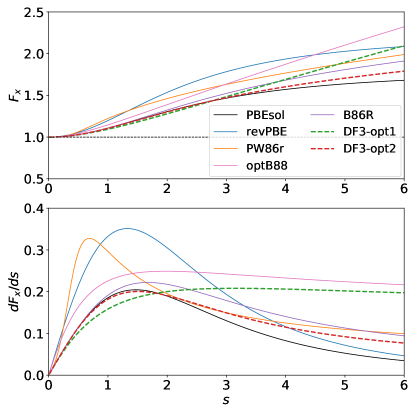
Figure 1: (top) Exchange enhancement factors $F_{\rm x}(s)$ and (bottom) their derivatives for selected functionals.

In vdW-DF1, revPBE exchange^{52; 53} was chosen as the GGA exchange. This choice was based on the fact that its rapidly increasing $F_{\rm x}(s)$ in the $s=0.5-2$ range, as shown in Fig. 1, ensures that nonphysical binding effects from the exchange energy are kept at a minimum.^{27; 42} However, the choice of revPBE also leads to a consistent overestimation of binding separations, occasionally causing incorrect bonding predictions.^{54; 55; 56; 32} After a number of studies had established both the capabilities and shortcomings of vdW-DF1,^{57; 58; 59; 60; 29; 61} the turn of the previous decade saw a string of important improvements. First, Murray et al. ⁴² demonstrated that a generally less rapidly but increasing $F_{\rm x}(s)$ for all values of $s$ (as well as in the asymptote) could also be used to avoid spurious binding from the exchange energy. They did so by reparameterizing the Perdew-Wang functional of 1986 (PW86r) ⁶² and showed that $F_{\rm x}(s)\propto s^{2/5}$ for large values of $s$ is well suited to reproduce the Hartree-Fock exchange interaction curves beyond binding separations. This insight was used in the design of the successor vdW-DF2 ⁴³ which utilizes PW86r exchange, but also changes an internal parameter from $Z_{ab}^{\text{DF1}}=-0.8491$ to $Z_{ab}^{\text{DF2}}=-1.887$. This switch effectively reduces the polarizability of a given density region, but more so for highly inhomogeneous low-density regions than for high density ones.⁶³ Through these changes, vdW-DF2 obtains a significantly improved accuracy for molecular dimers; however, for solids, layered systems, and some adsorption systems, the development did not resolve the overestimation issues of vdW-DF1, which in some cases even worsened.^{39; 30; 64; 65} This surprising worsening is possibly related to the fact that the derivative of $F_{\rm x}(s)$ of PW86r is larger than that of revPBE around $s=0.5$, see Fig. 1, as $dF_{\rm x}(s)/ds$ is linked to the force exerted by the repulsive wall.

Around the same time, Cooper³⁶ demonstrated that the systematic overestimation of binding separations could be avoided by using a “soft” exchange functional, i.e. having an exchange enhancement factor $F_{\rm x}(s)$ that increases slowly with $s$ for small values of $s<1$. Similarly, the exchange functionals optB86b³⁹ for vdW-DF1 correlation and B86R for vdW-DF2 correlation explicitly set the low-$s$ limit to that of the gradient expansion $\mu_{\rm GEA}$ used in the soft PBEsol,⁶⁷ resulting in significant improvements of lattice constants for solids. The various enhancement factors and their performance for different systems have been compared and analyzed in the context of vdW-DF in e.g. Refs. (42; 30; 50). To summarize, the following was learned. $\blacksquare$ Lesson 1: The specific shape of $F_{\rm x}(s)$ strongly impacts the bonding in vdW-DF and must be part of any functional design. The small-$s$ limit should be soft, i.e. similar to PBEsol ⁶⁷ in the small $s$ regime, to provide accurate solid lattice constants and $F_{\rm x}(s)$ should be asymptotically increasing (i.e. with a positive non-zero derivative in the asymptotic $s$ limit) rather than going to a constant to avoid spurious binding from the exchange energy. This insight was also used in the CX ⁴⁰ exchange functional designed for vdW-DF1 correlation. While several GGA functionals approach a constant value in the asymptote (such as PBE and PBEsol) or for large $s$ do not exhibit monotonically and asymptotically increasing $F_{\rm x}(s)$ (such as PW91⁶⁸), this continued increase is essential within the vdW-DF framework to avoid spurious binding stemming from the exchange part of the exchange-correlation functional.⁴² We also note that the analysis and discussion of $F_{\rm x}(s)$ as a function of $s$ has a long history, predating the vdW-DF development.^{69; 70; 71}

Instead of updating the non-empirical criteria used in the design of $F_{\rm x}(s)$, Klimes et al. ³⁷ fitted $F_{\rm x}(s)$ directly to the binding energies of the S22 data set of molecular dimers keeping the vdW-DF1 correlation fixed for a set of functional forms. These variants are therefore labeled as semi-empirical or “reference system optimized”. Their approach was surprisingly effective in the sense that it not only improved binding energies for molecular dimers, as would be expected, but also reduced the overestimation of binding energies and improved performance for several other classes of systems such as adsorption on coinage metals. This is in particular the case for the optB88 ³⁷ functional, which also arrived at a quite soft (i.e. slowly increasing with $s$) small-$s$ from, but a rapidly increasing high-$s$ form. This provides our next lesson. $\blacksquare$ Lesson 2: Within vdW-DF, reference-system optimization to specific benchmark sets has the potential to provide versatile functionals. A likely reason for this is the rigorously derived non-local correlation model of vdW-DF, which is based on exact constraints (see Section II.2). The fitting to reference data was also used successfully within the vdW-DF framework in the construction of BEEF-vdW.³⁸ Fitting to reference data is a common strategy in DFT functional development more generally, done extensively for example in the popular Minnesota functionals.^{72; 73}

As of today, the optB88, optB86b, and CX exchange for vdW-DF1 and B86R for vdW-DF2 are all actively used for broad classes of van der Waals bonded materials and all have quite comparable overall performance, with B86R possibly being slightly better for solids ⁶⁵ while optB88 is the only one providing satisfactory results for rare gas dimers.⁷⁴ $\blacksquare$ Lesson 3: It is not clear whether vdW-DF1 or vdW-DF2 correlation is the best starting point for designing improved functionals, but in any case a suitable exchange partner must be constructed once the correlation functional is updated. In addition, the similar performance of the best vdW-DF1 and vdW-DF2 variants indicate that tuning $Z_{ab}$ is not sufficient to greatly improve performance. We also note that both B88⁷⁵ and B86b⁷⁶ would be suitable starting points for reparameterizations of $F_{\rm x}(s)$. This is less true for CX, as it was designed solely for the vdW-DF1 correlation and is not as widely available in various codes, though this is being remedied.⁷⁷

Finally, in our recent work we found that tuning the momentum dependence of the plasmon-pole model within vdW-DF provides an additional degree of freedom that is fully consistent with the original constraint-based design philosophy and that can be used to tailor various aspects of the vdW-DF performance.⁵¹ In particular, we learned two important points. $\blacksquare$ Lesson 4: The plasmon-pole model is the key for improving the ability to simultaneously describe short- and long-range contributions to van der Waals interactions and thus also its ability to describe both small dimers and extended systems accurately. And, the asymptotic behavior of any vdW-DF functional has limited influence on the binding curves over physically relevant distances.

All these lessons laid the foundation for our design of vdW-DF3.

II.2 Review of the Original vdW-DF Framework

The kernel $\Phi(\mathbf{r},\mathbf{r^{\prime}})$ in Eq. (1) can be rigorously derived through a second-order expansion of the ACF. The expansion is in terms of an effective plasmon propagator $S$, which describes virtual charge-density fluctuations of the electron gas and has poles for real frequencies at the effective plasmon frequency $\omega_{\mathbf{q}}$, where $\mathbf{q}$ is the momentum of the plasmon.^{27; 30} Written explicitly including the kernel $\Phi(\mathbf{r},\mathbf{r^{\prime}})$, Eq. (1) takes the form:

$$E_{\rm c}^{\rm nl}[n] = \int_{0}^{\infty}\frac{du}{4\pi}\int\frac{d^{3}\mathbf{q}}{(2\pi)^{3}}\frac{d^{3}\mathbf{q}^{\prime}}{(2\pi)^{3}}\times$$ (3)

$$\big{[}1-(\hat{\mathbf{q}}\cdot\hat{\mathbf{q}}^{\prime})^{2}\big{]}\;S_{\mathbf{q},\mathbf{q^{\prime}}}({\rm i}u)S_{\mathbf{q}^{\prime},\mathbf{q}}({\rm i}u)\;,$$

where $S$ is given by:

$$S_{\mathbf{q},\mathbf{q^{\prime}}}({\rm i}u) = \frac{1}{2}\Big{[}\tilde{S}_{\mathbf{q},\mathbf{q^{\prime}}}({\rm i}u)+\tilde{S}_{-\mathbf{q^{\prime}},-\mathbf{q}}({\rm i}u)\Big{]}$$ (4a)

$$\tilde{S}_{\mathbf{q},\mathbf{q^{\prime}}}({\rm i}u) = \int\!d^{3}\mathbf{r}\;\frac{e^{-{\rm i}(\mathbf{q}-\mathbf{q}^{\prime})\cdot\mathbf{r}}\;4\pi n(\mathbf{r})}{\big{(}{\rm i}u+\omega_{\mathbf{q}}(\mathbf{r})\big{)}\big{(}(-{\rm i}u+\omega_{\mathbf{q^{\prime}}}(\mathbf{r})\big{)}}$$ (4b)

Here, $u=-{\rm i}\,\omega$ is the imaginary frequency and $4\pi n(\mathbf{r})$ is the square of the classical plasmon frequency. Note that there are two symmetric two-point $S$ in Eq. (3), each of which contains one density and one spatial integral (see Eq. (4b)), leading to the two densities and spatial integrals in Eq. (1). This particular form of $S$ is chosen such that it can fulfill four important physical constraints, i.e. time invariance, charge conversation, the $f$-sum rule, and maintaining self-correlation at large $q$.^{27; 30} These constrains are at the heart of vdW-DF and make it a powerful and transferable tool for capturing van der Waals interactions in vastly different systems.

As the main ingredient in Eq. (4b), the dispersion model for $\omega_{\mathbf{q}}$ comes into focus. The small-$q$ limit of $\omega_{\mathbf{q}}$ has to be a constant (i.e. independent of $q$). On the other hand, for the choice of $S$ in Eq. (4b), the above constraints are fulfilled if the plasmon dispersion has the large-$q$ limit of $\lim_{q\to\infty}\omega_{\mathbf{q}}(\mathbf{r})=q^{2}/2$. For $q$ values in-between, the dispersion is not known. As such vdW-DF uses a switching function $h$ that smoothly switches between the two known limits. In particular, vdW-DF defines for the plasmon dispersion

$$\omega_{\mathbf{q}}(\mathbf{r})=\frac{q^{2}}{2}\cdot\frac{1}{h\big{(}q/q_{0}(\mathbf{r})\big{)}}\;,$$ (5)

where the switching function $h$ determines the relation between density-density fluctuations and electromagnetic induction at different length scales. To facilitate the numerical evaluation, the vdW-DF framework uses only one length scale $\sim 1/q_{0}\big{(}n(\mathbf{r})\big{)}$ in the switching function, which depends on the density and parameterizes the local response of the electron gas. $q_{0}(\mathbf{r})$ is determined by the requirement that the first-order expansion of the ACF in $S$ reproduces a generalized gradient approximation-type local exchange-correlation (XC) functional. This XC functional is referred to as the internal functional, $\epsilon^{\rm int}_{\rm xc}$, and is in general different from the total exchange-correlation functional. The first-order expansion then yields for the internal functional²⁷

$$\epsilon^{\rm int}_{\rm xc}(\mathbf{r}) =\pi\int\frac{d^{3}\mathbf{q}}{(2\pi)^{3}}\left[\frac{1}{\omega_{\mathbf{q}}(\mathbf{r})}-\frac{2}{q^{2}}\right]$$

$$=2\pi\int\frac{d^{3}\mathbf{q}}{(2\pi)^{3}}\frac{1}{q^{2}}\left[h\big{(}q/q_{0}(\mathbf{r})\big{)}-1\right]$$

$$=-\frac{1}{\pi}\,q_{0}(\mathbf{r})\int_{0}^{\infty}dy\,[1-h(y)]\;.$$ (6)

If we set

$$\int_{0}^{\infty}dy\,[1-h(y)]=\frac{3}{4}\;,$$ (7)

then $q_{0}(\mathbf{r})$ takes a particularly simple form of a modulated Fermi wave vector $k_{\rm F}^{3}(\mathbf{r})=3\pi^{2}n(\mathbf{r})$, i.e. $q_{0}(\mathbf{r})=-(4\pi/3)\,\epsilon^{\rm int}_{\rm xc}(\mathbf{r})=\big{(}\epsilon^{\rm int}_{\rm xc}(\mathbf{r})/\epsilon_{\rm x}^{\rm LDA}(\mathbf{r})\big{)}\,k_{\rm F}(\mathbf{r})$. For practical purposes, the internal functional is approximated as LDA exchange correlation plus simple quadratic exchange gradient corrections of the form $-Z_{ab}^{\text{DF1(2)}}s^{2}/9$, which differ in vdW-DF1 and vdW-DF2 because their $Z_{ab}$ are different. Both these functionals represent two different directions for design philosophies and yield varying levels of accuracy for different classes of materials.³⁰

Obvious constraints on $h(y)$ are Eq. (7) and that $\lim_{y\to\infty}h(y)=1$ to fulfill the large-$q$ limit of $\omega_{\mathbf{q}}(\mathbf{r})$. A third constraint, i.e. $h(0)=0$, corresponds to charge conservation of the spherical XC hole model of the internal functional.⁴⁹ The original vdW-DF framework chooses a particular simple switching function that fulfills all of those constraints trivially as $h_{\rm orig}(y)=1-\exp(-\gamma y^{2})$, where $\gamma=4\pi/9$. However, the three constraints do still leave considerable freedom and more complicated forms of $h$ are conceivable—yet, staying completely within the original framework and thus inheriting its constraint-based transferability.

As a final point, the dispersion model for $\omega_{\mathbf{q}}$ increases with $q$, which effectively dampens the dispersion correction compared to the asymptotic response. Thus, tuning the dispersion model is somewhat reminiscent of optimizing damping functions in dispersion-correction schemes that start from an asymptotic formula.⁷⁸ However, there are important distinctions between damping in vdW-DF and dispersion-corrected methods or semi-empirical non-local correlation functionals such as VV10: In vdW-DF, the total non-local correlation has both short-range repulsion and long-range attraction components and the wiggle-room in possible dispersion models is highly constrained by the large-$q$ limit and the integral in Eq. (7).

II.3 New Development

We have recently demonstrated that the freedom in choosing the $h$ function can be exploited to significantly improve the notoriously bad $C_{6}$ coefficients that derive from the vdW-DF framework.⁵¹ From our work it became obvious that this newly found freedom directly translates into a significantly expanded design freedom (Lesson 4). Although our focus in Ref. (51) was on the asymptote, we nonetheless gained some general insight into what aspects of $h$ lead to what outcomes. In this regard, the fixing of the $C_{6}$ coefficients was a simpler task, as they are proportional to $\lim_{y\to 0}h(y)/y^{2}$; the problem of fixing the $C_{6}$ coefficients (asymptotic behavior) is thus separable from improving the binding (short-range behavior) and a relatively simple $h$ function is sufficient.

In our new development, we explore a larger space of $h$ functions in order to improve the general accuracy for short, medium, and long separations. This problem is vastly more complicated compared to the $C_{6}$ coefficients as it does not separate and competing interests have to be balanced. The accurate description of interactions beyond the binding separation is important for e.g. surface-molecule vibrations and related zero-point energies^{33; 79} as well as inter-layer binding and surface adsorption, for which it has been nicely demonstrated in Ref. (63)—in particular for non-planar molecules such as C₆₀.

Based on what we learned from our work on the $C_{6}$ coefficient, combined with an extensive amount of trial and error, we identified a new switching function which is both smooth and more flexible, in the form of

$$h(y)=1-\frac{1}{1+\gamma y^{2}+(\gamma^{2}-\beta)y^{4}+\alpha y^{8}}\;.$$ (8)

$\alpha$, $\beta$, and $\gamma$ are adjustable parameters in this model, albeit one of them is constrained by Eq. (7); we describe in Sec. II.4 how we determine the values of those parameters with the help of an optimization scheme (Lesson 2). This particular form of $h$ has a small-$y$ expansion of the form

$$h(y)=\gamma y^{2}-\beta y^{4}+(2\beta\gamma-\gamma^{3})y^{6}+\dots$$ (9)

or equivalently,

$$\omega_{\mathbf{q}}(\mathbf{r})\sim y^{2}/h(y)=$$

$$= 1/\gamma+\beta y^{2}/\gamma^{2}+(\beta^{2}/\gamma^{3}-2\beta/\gamma+\gamma)y^{4}+\dots$$

This allows a clear interpretation of the parameters, as the $\gamma$ parameter sets the long-range van der Waals interactions, whereas the $\beta$ parameter is the leading-order term causing damping of van der Waals interactions at shorter ranges. Finally, the $\alpha y^{8}$ term ensures that Eq. (7) can be fulfilled without interfering with the series expansions determining the long- and medium-range behavior of the functional. The particular form of $h$ is in part inspired by the so-called vdW-DF-09 from Vydrov and Voorhis,⁴⁶ which does not fulfill Eq. (7), and was designed just prior to the release of the more well-known VV09 and VV10.^{20; 22} Note that, while Eq. (II.3) does not contain the exponential term of the original $h$ function, it can be made into a form very similar to $h_{\rm orig}(y)$ in the more relevant $0<y<2$ range.

The $h$ function in Eq. (8) provides an independent parameter for the $y^{2}$ term in the series expansion of $\omega_{\mathbf{q}}(\mathbf{r})$, Eq. (II.3). This freedom can be beneficial for fine-tuning the strength of the van der Waals interactions in the mid-range, a few Å  away from the optimum binding separations. However, when trying to minimize the error in interaction energy of van der Waals complexes from binding distances to mid-range and larger distances, we find the somewhat surprising result that the optimal $\beta$ is close to 0, so that we actually approximate it with $\beta=0$. This simplifies Eqs. (8) – (II.3) and we thus define our $h$ function for vdW-DF3 as

$$h_{\rm DF3}(y)=1-\frac{1}{1+\gamma y^{2}+\gamma^{2}y^{4}+\alpha y^{8}}\;,$$ (11)

which leads to the small-$y$ expansions

$$h_{\rm DF3}(y) = \gamma y^{2}-\gamma^{3}y^{6}+\dots$$ (12)

$$y^{2}/h_{\rm DF3}(y) = 1/\gamma+\gamma y^{4}+\dots$$ (13)

The quadratic term in $y^{2}/h_{\rm DF3}(y)$ is absent, which correspond to the long-range limit of vdW-DF being well suited to describe the entire long-to-mid range van der Waals interactions; at the same time $\beta=0$ also allows a sharper damping of van der Waals interactions in the mid-to-short range because of a larger $\alpha$ term, corresponding to a faster increase of $h$ at $y\gtrsim 1$. Note that in this context “long-range” in our design does not correspond to the asymptotic limit, but rather corresponds to separations of about 5 – 6 Å beyond the optimum separation.

Figure 2 compares three different $h$ functions. Although all these switching functions appear very similar when plotted vs. $y$, a different picture emerges when plotting the physically relevant quantity $y^{2}/h(y)$, which shows stark difference for $y<0.8$. As both vdW-DF1 and vdW-DF2 correlation is in use in standard functionals today and their performance is comparable (Lesson 3), for our new functional form we want to explore possibilities for improvements both within the vdW-DF1 and vdW-DF2 design philosophies and thus present two different parameterizations, which we call $h_{\text{DF3-opt1}}$ and $h_{\text{DF3-opt2}}$. Both functions are nearly constant for $y^{2}/h_{\rm DF3}(y)$ within $0<y<0.3$, which is related to $\beta=0$. In contrast, for $h_{\rm orig}$ this function behaves quadratic for small $y$. All plotted $h$ functions have intercepts at different values $\lim_{y\to 0}y^{2}/h(y)=1/\gamma$ because they all have different values for $\gamma$. This intercept is directly related to the asymptotic behavior of the functional and different degrees of accuracy for the corresponding $C_{6}$ coefficients can thus be expected.⁵¹

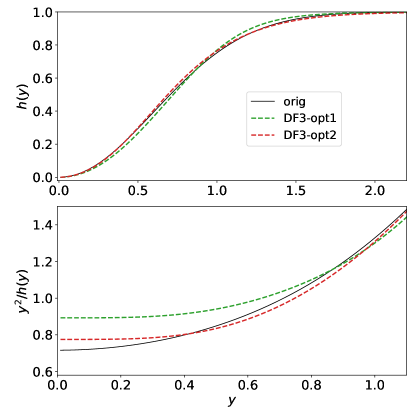
Figure 2: (top) Directly comparing the various $h$ functions shows only minimal changes. (bottom) Looking at $y^{2}/h(y)$, which is proportional to the plasmon dispersion $\omega_{\mathbf{q}}$, is much more revealing. The switching function $h_{\rm orig}$ is taken from Ref. (27). Note the different scales on the horizontal axes in both panels. The parameters for $h_{\text{DF3-opt1}}$ and $h_{\text{DF3-opt2}}$ in Eq. (11) are $(\alpha=0.94950,\gamma=1.12)$ and $(\alpha=0.28248,\gamma=1.29)$, respectively.

Our new switching functions $h_{\text{DF3-opt1}}$ and $h_{\text{DF3-opt2}}$ constitute a significant change of the original vdW-DF framework. Any such modifications require careful attention to rebalancing the exchange part in Eq. (2) (Lesson 1). As the exchange largely determines the local screening effects that characterize the chemical binding, we choose to rebalance it through a reparameterization of the free parameters within the enhancement factors $F_{\rm x}$(s) of a GGA-based exchange. Since $h_{\text{DF3-opt1}}$ and $h_{\text{DF3-opt2}}$ are noticeably different, they both need their own exchange reparameterization. Based on the requirements of the $s$ dependence of $F_{\rm x}$ (Lesson 1), we use

$$F_{\rm x}^{\text{DF3-opt1}}(s) = 1+\frac{\mu s^{2}}{1+\mu\,s\,\operatorname{arcsinh}(c\,s)/\kappa}$$ (14)

$$F_{\rm x}^{\text{DF3-opt2}}(s) = 1+\frac{\mu s^{2}}{(1+\mu s^{2}/\kappa)^{4/5}}\;,$$ (15)

where $c=2^{4/3}(3\pi^{2})^{1/3}$. These exchange functionals are inspired by optB88³⁷ and B86R,⁴¹ which have previously been paired successfully with vdW-DF1 and vdW-DF2. To describe ‘weakly homogeneous’ systems, such as solids, layered structures and surfaces, we choose $\mu=\mu_{\rm PBEsol}=10/81$ for both forms (Lesson 1). However, the larger density-gradient region $1<s<4$, which directly influences the non-local binding regions, needs to be optimized with respect to our new vdW-DF3 non-local functional, which we achieve through including $\kappa$ in our optimization scheme in Sec. II.4. Figure 1 shows the differences in the various enhancement factors and their first derivatives. In both cases, the enhancement factors and their derivatives are reduced at larger gradients ($1<s<4$), indicating that these semi-local exchange functionals become less repulsive at higher density gradients compared to the original functional forms that inspired them, i.e. optB88 and B86R. Finally, we note that both the $F_{\rm x}(s)$ of DF3-opt2 has a shape that is quite similar to that of B86R and $h(y)$ that is quite similar to that of the original vdW-DF, indicating the suitability of B86R for the vdW-DF2 correlation. DF3-opt1, on the other hand, has no such close similarity with previous functionals.

II.4 Optimization Scheme

Our original theoretical development leaves three adjustable parameters, i.e. $\beta$ and $\gamma$ from the proposed new switching function in Eq. (8)—we constrain $\alpha$ for every pair of $\beta$ and $\gamma$ through Eq. (7)—and $\kappa$ from the enhancement factor in Eqs. (14) and (15). Since there are two different enhancement factors with possibly different values for $\kappa$, in principle we have to perform two three-dimensional optimizations. We are using a reference-system optimization (Lesson 2), where our parameters are optimized with reference to high-level quantum chemistry (QC) results at the CCSD(T) level of the S22$\times$5 dataset.⁸⁰ The quantity to be minimized is the deviation of our calculated interaction energies from the CCDS(T) reference for all 22 systems and all 5 separations. To avoid making the optimization dominated by the large molecular dimers with large binding energies, the target to be minimized should be a relative rather than an absolute energy difference. In particular, we considered the following two measures: mean absolute relative deviation (MARD) and a differently weighted variant which we call weighted mean absolute relative deviation (WMARD), defined as

$${\rm MARD} = \frac{1}{n}\sum_{\rm sep=1}^{n}{\rm MARD_{sep}}\hskip 20.00003pt$$ (16)

$${\rm WMARD} = \frac{1}{n}\sum_{\rm sep=1}^{n}{\rm WMARD_{sep}}$$ (17)

where

$${\rm MARD_{sep}} = \frac{1}{m}\sum_{\rm sys=1}^{m}|E^{\rm DFT}_{\rm sys,sep}-E^{\rm QC}_{\rm sys,sep}|/E^{\rm QC}_{\rm sys,sep}\hskip 20.00003pt$$ (18)

$${\rm WMARD_{sep}} = \frac{1}{m}\sum_{\rm sys=1}^{m}|E^{\rm DFT}_{\rm sys,sep}-E^{\rm QC}_{\rm sys,sep}|/E^{\rm QC}_{\rm sys,opt}$$ (19)

For the S22$\times$5 set used in our optimization we have $n=5$ and $m=22$. Note that MARD puts the deviation in relation to the QC result at that separation and thus treats all separations on the same basis. However, when using MARD we found that the optimization equally weights large percentage deviations at large separations, which, however, may on the absolute scale only be in the sub-meV range—to the detriment of performance around the binding separation. We thus weigh the deviation by the interaction energy at the optimal separation, $E^{\rm QC}_{\rm sys,opt}$ (where “opt” is the one separation out of the five for which the interaction energy is largest), and optimize WMARD instead.

Table 1: Optimum parameters for vdW-DF3-opt1 and vdW-DF3-opt2. We set $\beta$ to zero and constrained $\alpha$ through Eq. (7), leaving only $\gamma$ and $\kappa$ as adjustable parameters.

functional	$Z_{ab}$	$h$ function	$\alpha$	$\beta$	$\gamma$	exchange	form	$\kappa$	$\mu$
DF3-opt1	$Z_{ab}^{\text{DF1}}=-0.8491$	$h_{\text{DF3}}$	0.94950	0	1.12	$F_{\rm x}^{\text{DF3-opt1}}$	B8875	1.10	$\mu_{\rm PBEsol}$ = 10/81
DF3-opt2	$Z_{ab}^{\text{DF2}}=-1.887$	$h_{\text{DF3}}$	0.28248	0	1.29	$F_{\rm x}^{\text{DF3-opt2}}$	B86b76	0.58	$\mu_{\rm PBEsol}$ = 10/81

The optimization is now performed on a grid for all three parameters, where we use a coarse grid at first and later a finer grid around the minimum. Note that each point in this three-dimensional space requires $22\times 5+22\times 2=154$ (dimers + monomers) calculations, which quickly becomes cost prohibitive. We thus decouple the exchange degree of freedom from the $h$-function degrees of freedom and transform the three dimensional optimization into a one-dimensional and two-dimensional optimization. This can be achieved through performing non-selfconsistent calculations and extracting the exchange energy as a function of $\kappa$ (which is almost entirely independent of $\beta$ and $\gamma$) and the non-local correlation as a function of $\beta$ and $\gamma$ (which also to a good approximation can be viewed as independent of $\kappa$). The total energy of any point in the three-dimensional space can then be reconstructed by adding the various contributions on the fly to optimize WMARD. In the end, we verified all our results with fully self-consistent calculations and our numbers reported here in all tables and figures are the results of fully self-consistent calculations. Although this approach constitutes a tremendous reduction in computational effort, we still performed roughly 50,000 non-selfconsistent calculations.

As mentioned in the previous section, we found optimized $\beta$ values that are a small positive number and zero for DF3-opt1 and DF3-opt2, respectively, so we chose to set $\beta=0$ and thus reduce the amount of parameters in our functionals down to two. Our optimized values for $\alpha$, $\gamma$, and $\kappa$ are collected in Table 1. It is conceivable that the global WMARD minimum, in particular for DF3-opt2, might occur for negative $\beta$, but this breaks formal constraints of the vdW-DF construction. Even though $\beta$ came out to be zero, we chose to present our formalism including $\beta$ as this additional parameter could be important in the design of vdW-DF3 variants based on broader benchmark sets, or perhaps in the construction of special-purpose functionals (in combination with carefully selected exchange functionals) such as for the description of molecular crystals⁸² or surface adsorption processes of importance to catalysis.⁸³

III Computational Details

All our calculations were performed with the quantum espresso (QE) package,⁸⁴ where we modified the kernel generation routines to implement our new functionals vdW-DF3-opt1 and vdW-DF3-opt2; these functionals are now available in the latest official version of QE. We used PBE GBRV ultrasoft pseudopotentials because of their excellent transferability.⁸⁵ The wave-function and density cutoffs were set to $\sim$680 eV (50 Ryd) and $\sim$8200 eV (600 Ryd), respectively. Self-consistent calculations were performed with an energy convergence criterion of $\sim$1.36$\times 10^{-7}$ eV ($1\times 10^{-8}$ Ryd) and, where applicable, a force convergence criterion of $\sim$2.6$\times 10^{-5}$ eV/Å ($1\times 10^{-6}$ Ryd/Bohr) was used for structure relaxations. For all calculations including metals/semiconductors a Gaussian smearing with a spread of $\sim$100 meV (7.35 mRyd) was used. Benchmarking of our new functionals has been done on the molecular dimer datasets S22$\times$5 and S66$\times$8, the G2–1 and G2RC sets, a set of solids, layered structures, molecular crystals, and benzene adsorption on Cu/Ag/Au surfaces. We compare the performance of our new functionals with other, well-used dispersion-corrected exchange-correlation functionals such as vdW-DF (vdW-DF1),²⁷ vdW-DF1-optB88,³⁷ vdW-DF1-cx,^{40; 32} vdW-DF2,⁴³ vdW-DF2-B86R,⁴¹ rVV10,⁸⁶ and SCAN+rVV10,⁸⁷ and we use the following corresponding short names in all tables and figures: DF1, DF1-optB88, DF1-cx, DF2, DF2-B86R, VV, and SCAN+VV, respectively. For the molecular dimers, we calculated all SCAN+VV values; for solids, layered structures, and adsorption on coinage metals we took readily available values from the literature, but for our molecular crystals we found no published SCAN+VV data.

For calculations on the dimer sets, spurious interactions due to the period boundary conditions in QE were minimized by padding dimers and monomers with at least 15 Å of vacuum. A list of 22 metals, semiconductors, and ionic salts were also used as in Ref. (39) except Li. A $15\times 15\times 15$ $k$-point mesh was used for these periodic solids. To calculate their lattice constants and cohesive energies, a Birch-Murnaghan equation-of-state was used and the individual atom energies were calculated in a box surrounded by at least 15 Å of vacuum. Results for cohesive energies and lattice constants are in addition compared to PBE⁸⁸ and PBEsol.⁶⁷ The reference data on zero-point corrected experimental lattice constants and atomization energies are taken from Ref. (39) and references therein. Several layered structures were also considered. Experimental structures were retrieved from the Inorganic Crystal Structure Database (ICSD). Following the procedure in Refs. (87; 89; 90), these layered structures were relaxed along the inter-layer axis ($c$-axis) with $12\times 12\times 6$ $k$-points, keeping the $a$-lattice constant at its experimental value. Inter-layer binding energies have been calculated using single layers with fixed $a$-lattice constant and with at least 12 Å vacuum along the $c$-axis, using a $12\times 12\times 1$ $k$-mesh. The corresponding reference data is taken from RPA calculations in Ref. (90) and references therein. The molecular crystal dataset X23 was also studied. Here, calculations were performed starting from structures provided in Ref. (91), followed by an optimization of all structural degrees of freedom. Finally, benzene adsorption on the (111) surface of the coinage metals Cu, Ag, and Au have also been used as a benchmark, using the reference data in Refs. (92; 93; 94; 95; 87). Six layers were used to form the metallic slab,⁹² keeping the three bottom layers fixed and using a 9 Å vacuum. Calculations were performed with a $4\times 4\times 1$ $k$-mesh.

IV Results

To investigate the performance of vdW-DF3-opt1 and vdW-DF3-opt2, we benchmark those functionals on an extensive list of systems reaching from molecular dimers to periodic systems including solids, layered systems, molecular crystals, and surface adsorption on coinage metals. We compare our results with the most popular functionals, finding good performance in general for a wide array of systems and a significant improvement in accuracy at larger separations.

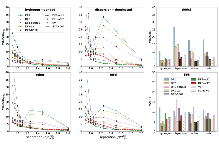
Figure 3: Statistical analysis for the S66$\times$8 and S66 datasets in reference to QC data at the CCSD(T) level. The four left figures show WMARD_sep from Eq. (19), summed over different S66$\times$8 subgroups. Separation is given in units of the optimal QC separation $d^{\rm QC}_{\rm opt}$. The top right panel shows WMARD from Eq. (17). The bottom right plot shows MARD for the optimal binding energy of the S66 dataset. We compare our results also to VV and SCAN+VV, but we separate them as they are fundamentally different approaches and should not be understood as improvements within the vdW-DF family.

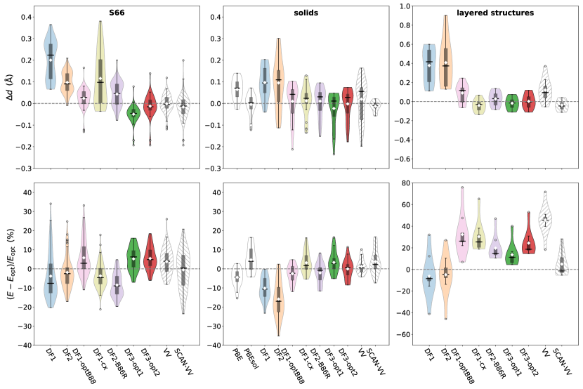
Figure 4: Violin plots overlaid on box plots of the deviations from reference data for the different functionals. Violin plots represent the data distribution and are based on a Gaussian kernel density estimation using the Scott’s rule,⁹⁶ as implemented in matplotlib. In the box plot, the boxes hold 50% of the data, with equal number of data points above and below the median deviation (full black line). Whiskers indicate the range of data falling within 1.5 $\times$ box-length beyond the upper and lower limits of the box. Outliers beyond this range are indicated with circular makers. Diamonds mark the mean deviation. (left) Set of 66 molecular dimers: reference data taken from CCSD(T);⁹⁷ results in terms of $d$ (dimer separation) and $E_{\rm opt}$ (binding energy). (middle) Set of 22 solids: reference data taken from zero-point corrected experiments;⁹⁸ $d$ refers to lattice constant and $E_{\rm opt}$ to atomization energy. (right) Set of 9 layered structures: reference data taken from RPA calculations;^{89; 90} $d$ refers to layer separation and $E_{\rm opt}$ to layer binding energy. SCAN+VV data for solids and layered structures taken from Ref. (87).

IV.1 Molecular Systems

The two adjustable parameters of our functionals (see Table 1) have been fitted to minimize the WMARD of the S22$\times$5 dataset,⁸⁰ as described in Sec. II.4. A comparison for this dataset is thus biased by construction and we will not go into extensive details here. Appendix A holds a statistical summary and detailed results for each dimer are provided in the Supporting Information. Overall, both our new functionals have a WMARD of less than 4% and perform best in our comparison group. The performance is particularly good for dispersion-dominated complexes. Even though we optimized WMARD, MARD also shows significant improvements.

The more diverse and larger S66$\times$8 set of molecular dimers is our first proper benchmark.⁹⁷ Similar to S22$\times$5, this set is comprised of 23 hydrogen bonded complexes, 23 dispersion-dominated complexes, and 20 complexes with various other kinds of interactions. Interaction energies at the CCSD(T) level are reported for eight different separations—two at separations below the optimal binding distance, one at the optimal binding distance, and five separations that are larger, up to twice the optimal binding separation. The WMARD defined in Eq. (17) for the S66$\times$8 set is given in the upper right panel of Fig. 3; a summary of statistical information can be found in Appendix A and detailed results for each dimer are provided in the Supporting Information. As S66$\times$8 is quite similar to the S22$\times$5 set, our two functionals also here perform best with a WMARD of 4.7% and 4.9%, although it has gone up by approximately one percentile. For dispersion dominated and mixed complexes DF3-opt1 performs better than all other tested with a WMARD of 4.7% and 3.5%, respectively. DF3-opt2 has slightly higher WMARD for dispersion-dominated system (6.2%), but is also very accurate (3.7%) for mixed complexes.

A more detailed picture of the performance for the S66$\times$8 emerges in Fig. 3, which provides WMARD_sep from Eq. (19), summed over all three subgroups as well as for all 66 complexes. The plots reveal that both DF3-opt1 and DF3-opt2 accurately describe interaction energies at equilibrium separation and beyond for each interaction type. In particular, we consider the “dispersion-dominated” panel amongst the most pertinent results of our study. It shows that DF3-opt1, and to a somewhat lesser extent DF3-opt2, agrees well with the quantum-chemical reference data for dispersion-bound systems beyond equilibrium separations—whereas several popular functionals give quite large errors in this regime—and thus confirms that we have achieved our goal of overcoming this longstanding problem. For hydrogen-bonded systems DF3-opt1 turns out to be less accurate than DF1-cx, DF2-B86R, and DF1-optB88 around the binding separation, but still has good performance similar to SCAN+VV and VV and shows a significant improvement over vdW-DF1 and PBE+D3.⁹⁹ DF3-opt2 shows an accuracy quite similar to DF3-opt1, but with somewhat better performance for hydrogen-bonded systems and short separations, at the cost of lower accuracy for dispersion-dominated systems. The reason that DF3-opt1 (and to a lesser extent DF3-opt2) is less accurate for hydrogen-bonded systems around the binding separation may be related to the smaller $dF_{\rm x}(s)/ds$ at around $s\approx 0.5-2$ compared to e.g. B86R or optB88.⁴⁰ Our analysis of $s$ values shows that this range is the most relevant for binding in hydrogen-bonded molecular dimers. Furthermore, a comparison of various forms of $F_{\rm x}(s)$ and $dF_{\rm x}(s)/ds$ and their influence on performance for different systems and types of interactions has been done in e.g. Refs. (42; 30; 50). In addition, in Section V we provide further discussion on the inherent trade-offs in vdW-DF design and give arguments that increased values of $dF_{\rm x}(s)/ds$ in this range can improve performance for hydrogen-bonded systems.

In addition, we also provide data for the S66 data set,⁹⁷ which contains the same molecular dimers as the S66$\times$8 set but uses the optimal binding separation rather than looking at eight explicit separations. Thus, in our comparison, we also fully optimize the binding separation with the various functionals. The MARD of the resulting optimized binding energies is given in the bottom right panel of Fig. 3 and statistical data for the deviations in optimal binding separation and binding energy are analyzed in the left column of Fig. 4 in the form of violin plots and box plots; additional data is available in the Supporting Information. Again, we find that DF3-opt1 and DF3-opt2 perform very well. In particular, the violin plots reveal that our new functionals provide rather compact results with less spread in comparison to other functionals.

As a simple check that our reparameterization of the non-local correlation and semilocal exchange does not cause vdW-DF3 to fail in basic chemistry areas, we test our two functionals for the G2–1^{100; 101} set of molecular atomization energies as well as the G2RC¹⁰¹ set for reaction energies. Results are depicted in Fig. 5; additional information is available in Appendix A and the Supporting Information. Most functionals perform similar for both tests—typically comparable to PBE as expected¹⁰² and better than PBEsol—with small deviations in spread and mean/median.

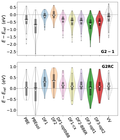
Figure 5: Violin plots of deviations for the atomization energies of the G2–1 set and reaction energies of the G2RC set. Reference data taken from Refs. (103; 104). See caption of Fig. 4 for further details.

IV.2 Solids

Within DF3-opt1 and DF3-opt2 the non-local correlation is purposefully combined with an exchange energy that has a smaller, PBEsol-like enhancement factor for small $s$, i.e. $F_{\rm x}^{\text{DF3-opt}}(s)=1+\mu_{\rm PBEsol}s^{2}+\dots$, which significantly improves lattice constants of solids. In Fig. 4 we collect statistical information in the form of violin plots combined with box plots for a set of 22 standard solids and provide deviations for lattice constants and atomization energies. As reference we use results from zero-point corrected experiments.⁹⁸ Further numerical data is provided in Appendix A. Clearly, PBEsol and SCAN+VV provide an accurate description of lattice constants. However, DF3-opt1 and DF3-opt2, together with other recent functionals also show good performance. In terms of atomization energies, we find several functionals that perform well and even better than PBE, including our new functionals. In particular, DF3-opt2 has a mean and median deviation of essentially zero. Within the vdW-DF family of functionals, DF3-opt1 and DF3-opt2 retain this significant advancement in vdW-DF design, as the original functionals DF1 and DF2 both overestimate lattice constants for solids.

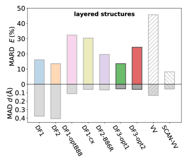
Figure 6: MARD of layer binding energy and MAD of layer separation for a set of layered structures. SCAN+VV data taken from Ref. (87).

IV.3 Layered Structures

We also benchmark our functionals for a set of 9 layered structures against RPA reference calculations^{89; 90} and results are given in the right column of Fig. 4. Futher details are provided in Appendix A, also see Ref. (65). While the original DF1 and DF2 significantly overestimate the layer separation, much improvement can be seen for all other vdW-DF functionals. In particular, DF3-opt2 has a mean deviation of zero and a compact spread, closely followed by DF3-opt1. Improvements for the layer binding energy are mostly observed in smaller spreads for newer vdW-DF functionals. While SCAN+VV is remarkably accurate for these systems, DF3-opt1 performs best out of all vdW-DF functionals. The progress made by our two functionals within the vdW-DF family can better be seen in Fig. 6, where we show the MARD of layer binding energy and MAD of layer separation. The original DF1 and DF2 functionals had a reasonable MARD for the energy, but their MAD in layer separation rendered them inapplicable for layered structures. Further developments like DF1-optB88, DF1-cx, and DF2-B86R corrected that behavior, but to the detriment of MARD in energy. DF3-opt1 now noticeably reduces the MARD in energy again (and also the spread, see Fig. 4) while having the lowest MAD in layer separation of any tested functional.

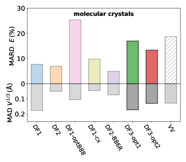
Figure 7: MARD of the cohesive energy per monomer (with respect to separation into molecules) and MAD of the third-root volume for the X23 dataset of molecular crystals.

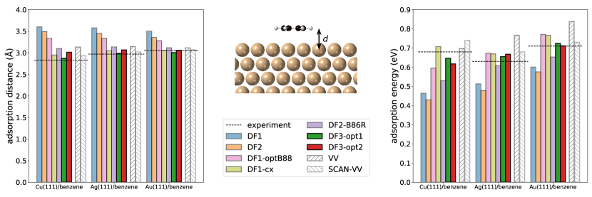
Figure 8: (left) Adsorption distance (Å) and (right) adsorption energy (eV) for benzene on Cu, Ag, and Au. Experimental reference values are taken from Ref. (95). The inset shows the adsorption geometry.

IV.4 Molecular Crystals

An important benchmark for all van der Waals functionals are molecular crystals.^{30; 106; 12; 65; 107; 108; 82; 91} We have calculated the optimized volume and the cohesive energy per monomer (with respect to separation into molecules) for the X23 dataset of molecular crystals.¹⁰⁹ Results are depicted in Fig. 7; a summary of statistical data is available in Appendix A and detailed results for each crystal are provided in the Supporting Information. Looking at the third-root volume (as an average representative of lattice constants), we see that our vdW-DF3 functionals are comparable to VV and DF1, but they are less accurate than the other functionals. For the cohesive energy, our functionals are noticeably more accurate than DF1-optB88 and somewhat better that VV. Nonetheless, we do not recommend our two vdW-DF3 functional variants for molecular crystals, as better options are available. The underestimation of vdW-DF3 volumes can be linked to the shape of $F_{\rm x}(s)$ and $dF_{\rm x}(s)/ds$ as shown in Ref. (82) and is the result of a conscious trade-off we made for our $\kappa$ values in Eqs. (14) and (15), see the discussion in Section V. For the underestimation of cohesive energies, we speculate that the enhancement factor also plays an important role, but other well-known effects such as the delocalization error may also contribute—again, see Section V for more discussion. Although molecular crystals are bound by much the same interactions as present in our fitting set, the relative spatial configurations/orientations between molecules in the X23 can differ from those present in the S22$\times$5 and molecular crystals are denser in the sense that the average shortest distances between molecules in S22 is 13% larger than in the X23 set. In addition, many-body dispersion effects play a significant role in the molecular crystals of the X23 set, while they are rather small in molecular dimers.¹¹⁰

IV.5 Benzene Adsorption on Cu/Ag/Au (111)

Finally, we benchmark our new functionals also against molecular adsorption on coinage metals, which are challenging systems.³² In particular, we study the adsorption of benzene on the (111) surface of Cu, Ag, and Au. A summary of statistical data is available in Appendix A. In Fig. 8 we show the benzene adsorption distance from the surface and its adsorption energy and we see that the original DF1 and DF2 functionals significantly overestimate the binding separations, resulting in dramatic consequences for surface corrugation.⁷⁹ This figure also shows nicely the progress that has been made within the vdW-DF family, with DF3-opt1 providing distances that are almost spot-on the reference data and very accurate energies, closely followed by DF3-opt2. This good performance could be related to the excellence performance for dispersion-dominated systems in Fig. 3 for larger-than-binding separations. The adsorbed molecule interacts with the surface through dispersion forces not only with its footprint directly vertically underneath at typical binding distances, but also with the horizontally surrounding surface at larger-than-binding separations—and this is where our new functionals excel. The importance of such horizontal interactions beyond-binding separations has been demonstrated in Ref. (63). This aspect is also intimately linked to—and paralleled by—our improved performance for layered systems.

V Balancing Competing Interests — What can be Expected from the vdW-DF Framework?

The results in the previous sections showed that our new functionals vdW-DF3-opt1 and vdW-DF3-opt2 perform very well. The main advancement is the greatly increased performance for dispersion-dominated molecular dimers, especially at larger-than-binding separations, see Fig. 3. Although we also see improved and generally good performance for many other systems, we would like to point out that performance—although still good and comparable to SCAN+VV and VV and better than vdW-DF1 and PBE+D3—is somewhat less accurate for hydrogen-bonded systems at their equilibrium separation.

We have noticed this trend early on and investigated measures to also achieve highly accurate performance for hydrogen-bonded systems at the equilibrium separation. These systems are very much controlled by the choice of exchange and we have investigated further parameterized versions of Eq. (14), where changing $c$ in conjunction with $\kappa$ would, in fact, lead exactly to the desired improvement and we see good performance for hydrogen-bonded dimers around the equilibrium separation and molecular crystals. However, through this higher dimensional parameter search (and other avenues we have investigated) we learned an important lesson: With our new development, the overall vdW-DF framework is coming to its performance limits. Although possible new $h$-functions provide additional degrees of freedom that allow for improvements of many aspects of particular systems, we now see that further improvements are only possible to the detriment of other areas. In our case, improving the hydrogen-bonded systems at binding separation would lead to a decrease in accuracy for dispersion bound dimers, layered systems, and surface adsorption.

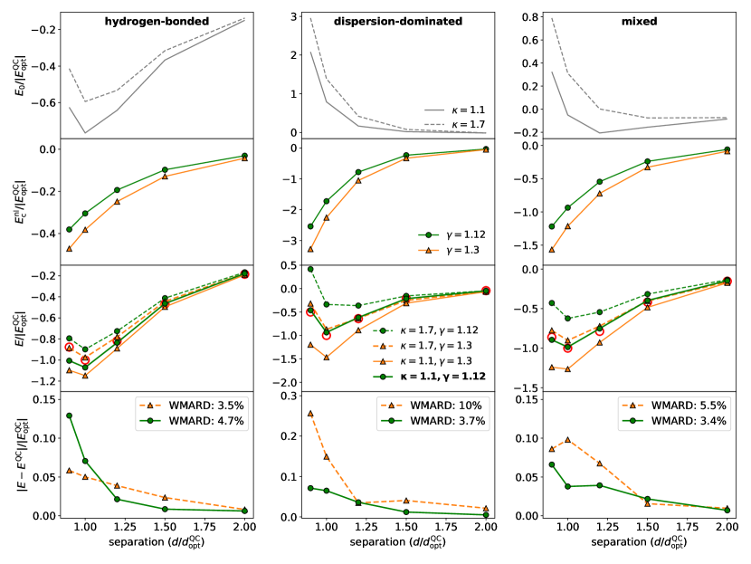
Figure 9: Split-up of the total energy into its non-local contribution (first row) and the rest (second row), i.e. $E=E_{\rm c}^{\rm nl}+E_{0}$ (third row), averaged over hydrogen-bonded, dispersion-dominated, and mixed dimers of the S22$\times$5 dataset. All energies are reported relative to the QC energy at the optimal separation $E_{\rm opt}^{\rm QC}$ and have been averaged over all dimers in that set. In the third row, QC reference data are indicated by red circles. Curves in third row combine the style from the top panel and color from the middle panel. In the fourth row, we show ${\rm WMARD_{sep}}$ from Eq. (19) for DF3-opt1 with $\kappa=1.1$/$\gamma=1.12$ and the functional with $\kappa=1.7$/$\gamma=1.3$; the legend gives the mean over all five distances.

We show in Fig. 9 how the balancing of competing interests plays out for the case of hydrogen-bonded molecular dimers vs. dispersion-dominated molecular dimers in Fig. 3. In particular, we study the split-up of the total energy into its non-local contribution $E_{\rm c}^{\rm nl}$ and the rest $E_{0}$, i.e. $E=E_{\rm c}^{\rm nl}+E_{0}$. Figure 9 shows this split-up as a function of our parameters $\kappa$ and $\gamma$. Our choice for DF3-opt1 was $\kappa=1.1$/$\gamma=1.12$, leading to very good performance for dispersion-dominated systems and somewhat less accuracy for hydrogen-bonded systems around and below the binding separation. However, we see that a choice of $\kappa=1.7$/$\gamma=1.3$ would have reversed those roles. In the Supporting Information we show the shape of $F_{\rm x}(s)$ and $dF_{\rm x}(s)/ds$ for the $\kappa=1.7$ parameterization in comparison to the ones in Fig. 1—one can see that the derivative starts to be noticeably larger for $\kappa=1.7$ compared to $\kappa=1.1$ for $s>0.5$. The choice of optimizing WMARD of the S$22\times 5$ set as described in Sec. II.4 resulted in dispersion-bonded systems being favored at the expensive of hydrogen-bonded systems. This is because the dispersion part is far more sensitive to the parameter choice for the dispersion-bonded systems, as can be seen in Fig. 9. The hydrogen-bonded part of WMARD is also significantly smaller in magnitude compared to the dispersion-dominated part. Our choice is in line with the fact that dispersion-bonded systems were the original target of the vdW-DF development and because of their impact on a large class of relevant problems in surface adsorption and layered structures. We speculate that our choice of $\kappa$ in vdW-DF3-opt1 and vdW-DF3-opt2 is also responsible for the lower accuracy in molecular crystals. We note in this context that the overall MAD of the S$22\times 5$ set is in fact smaller for $\kappa=1.7$/$\gamma=1.3$, i.e. 11.0 meV compared to 13.2 meV for vdW-DF3-opt1, but the latter has a considerable smaller MARD, i.e. 8.3% compared to 18.6% for $\kappa=1.7$/$\gamma=1.3$. Finally, the fourth column of Fig. 9 highlights the reasons for our choice of $\kappa$ and $\gamma$: While better performance in terms of WMARD could have been achieved for hydrogen-bonded systems with a choice of $\kappa=1.7$/$\gamma=1.3$, that same choice would result in noticeably reduced performance for dispersion-dominated and mixed systems (see legend of fourth row in Fig. 9).

To describe van der Waals interactions and non-covalent interactions beyond van der Waals interactions—in particular halogen- and hydrogen-bonded systems—with high accuracy at the same time is a long-standing problem within DFT and has been linked to the delocalization error resulting from incomplete self-interaction correction.^{111; 112; 113} This error is present in vdW-DF through the choice of (semi)local exchange and correlation and it is conceivable that the trade-off and reduced accuracy in certain systems are related to this error. Recently, a BEEF-vdW+$U$ method has been developed that tries to counteract the delocalization error through a Hubbard $U$ type correction and does indeed show improved results, albeit for strongly correlated systems where the error is more prominent.¹¹⁴ In this context, we would also like to point out that PBE+D3⁷⁸ has good performance for molecular dimers⁹⁹ and at the same time very good performance for molecular crystals, see Ref. (109) and the Supporting Information for a comparison. This points towards a particular quality of PBE+D3 that is capable to overcome the trade-off inherent in vdW-DF. Reference (115) shows that the good MARD for cohesive energies of PBE+D3 for molecular crystals almost triples to 16%—quite comparable to vdW-DF3—when higher multipole interactions are neglected, giving important insight that may help future vdW-DF developments. PBE+D3 does, however, have difficulties with surface adsorption and layered structures.^{65; 116}

Through the various improvements of the vdW-DF framework over the years we have reached a point where the performance of the original vdW-DF framework has been pushed to its limit and the fundamental design choices are now becoming the bottleneck. We see three exciting ways forward: (i) the inclusion of some fraction of exact exchange in the pairing with the vdW-DF non-local correlation. This is already ongoing work and shows promise.^{102; 117} This approach has the potential to overcome the current trade-off we encountered between hydrogen-bonded systems and dispersion-dominated systems—in particular with the additional degree of freedom in $h(y)$—and also provides a systematic improvement of the delocalization error.¹¹³ (ii) New functionals within the vdW-DF family could be developed for specific applications, rebalancing our choice. Such functionals would be somewhat limited in scope, but can show very good accuracy for the situation they have been designed for. Applications of particular interest may be adsorption systems, molecular crystals, or transition-state theory calculations. (iii) Alternatively, it is possible to fundamentally change the vdW-DF framework and deviate from its original design philosophy. We see this as the only option to achieve high accuracy for all systems at the same time and thus truly generate a general-purpose functional. So, where would one even start thinking about such a fundamental change? Below Eq. (5) we point out that vdW-DF uses only a single length-scale to parameterize its plasmon-dispersion model. Already in the 2004 paper we see that this is an approximation made for convenience,²⁷ and the introduction of a second length scale would be beneficial. It is, in fact, surprising that the vdW-DF framework captures such a diverse group of vastly different types of materials so reasonably well. Another possible direction could be to update the rather simple vdW-DF plasmon-dispersion model altogether, maybe along the lines of the VV functionals, from which much can be learned. Finally, it is conceivable that a focus on different physical constraints leads to a more accurate form for $S$ in Eq. (4a) or maybe $S$ could be approximated through better models for the response function. However, common to several of these directions would be that they fundamentally change the vdW-DF framework and design philosophy to such a point that they present completely new directions and thus would likely no longer carry the original vdW-DF name.

VI Conclusions

We have presented the next-generation non-local van der Waals density functional vdW-DF3. It is entirely built within the design guidelines of the original vdW-DF, but takes advantage of a newly discovered degree of freedom within the framework to significantly improve performance, in particular for beyond-binding separations. At the same time, we show that—by observing the vdW-DF constraints and building on lessons learned in successive developments—vdW-DF3 can retain the same wide transferability as earlier variants. This finding is based on benchmarking on a wide array of systems, in which we also compare with earlier van der Waals functionals, allowing us to document successive improvements. While we find generally good performance of vdW-DF3 for many systems, the most striking improvement is found for dispersion-dominated systems beyond binding separation. Our analysis also indicates that, with recent developments in general and vdW-DF3 in particular, the vdW-DF framework is operating close to its limits in terms of overall accuracy. This is also evident through the similarity of the DF3-opt2 parametrization of vdW-DF3 and the DF2-B86R functional. However, as the vdW-DF3 design is more flexible than its predecessors, it opens the door for functionals tailored to more specific classes of systems, which will likely cause some worsening in other areas. Finally, we provide an outlook for research directions that could overcome the fundamental bottlenecks of the vdW-DF framework and lead to further improvements for even broader classes of systems.

Appendix A Statistical Data

Table 2: Comparison of mean deviation (MD), mean absolute deviation (MAD), mean absolute relative deviation (MARD) from Eq. (16) and weighted mean absolute relative deviation (WMARD) from Eq. (17) for the interaction energies of the S22$\times$5 set of molecular dimers for all separations. Deviations are reported with respect to quantum chemistry calculations at the CCSD(T) level from Ref. (80).

Complex	DF1	DF2	DF1-optb88	DF1-cx	DF2-B86R	DF3-opt1	DF3-opt2	VV	SCAN-VV
Hydrogen bonded complexes (7)
MD [meV]	54.05	31.27	0.84	10.53	9.09	$-$24.26	$-$12.01	$-$18.84	$-$21.11
MAD [meV]	60.71	34.48	9.40	17.55	11.00	28.42	14.29	20.02	28.75
MARD [%]	14.36	7.01	3.17	6.28	3.02	6.25	3.81	5.11	7.41
WMARD [%]	11.04	5.63	2.17	4.00	2.08	4.72	2.64	3.83	4.71
Complexes with predominant dispersion contribution (8)
MD [meV]	29.40	30.84	$-$6.23	2.99	21.57	4.67	3.99	12.75	14.14
MAD [meV]	58.14	36.82	14.59	26.04	21.77	6.25	5.78	15.23	15.12
MARD [%]	135.84	74.36	41.29	67.94	42.88	12.44	13.98	33.09	67.42
WMARD [%]	32.78	17.88	9.92	18.82	13.23	3.67	3.69	7.32	10.11
Mixed complexes (7)
MD [meV]	17.40	19.25	1.96	5.58	16.00	3.15	3.89	6.60	6.24
MAD [meV]	28.61	19.91	6.67	15.23	16.07	5.91	5.54	7.73	10.34
MARD [%]	26.29	15.10	8.35	17.08	12.24	5.71	6.47	7.12	12.55
WMARD [%]	16.97	11.06	4.30	9.24	8.94	3.62	3.51	4.84	6.56
Average over all separation for all complexes (22)
MD [meV]	33.43	27.29	$-$1.37	6.21	15.83	$-$5.02	$-$1.13	0.74	0.41
MAD [meV]	49.56	30.70	10.42	19.90	16.53	13.19	8.41	14.37	17.94
MARD [%]	62.33	34.08	18.68	32.14	20.45	8.33	8.35	15.92	30.87
WMARD [%]	20.83	11.81	5.67	11.06	8.32	3.99	3.30	5.42	7.26

Table 3: Comparison of various statistical measures for the interaction energies of the S66$\times$8 set of molecular dimers for all separations. See caption of Table 2 for more details. Reference data taken from Ref. (97).

System	DF1	DF2	DF1-optb88	DF1-cx	DF2-B86R	DF3-op1	DF3-opt2	VV	SCAN-VV
Hydrogen bonded complexes (23)
MD [meV]	32.88	12.81	$-$3.01	6.47	4.32	$-$21.20	$-$14.89	$-$17.43	$-$18.08
MAD [meV]	39.45	17.44	7.29	13.87	9.00	22.19	15.27	17.89	20.65
MARD [%]	12.92	4.85	3.36	6.40	3.13	6.46	5.47	5.74	6.27
WMARD [%]	10.00	3.94	2.22	4.12	2.53	5.79	4.60	4.98	5.04
Complexes with predominant dispersion contribution (23)
MD [meV]	7.65	7.52	$-$17.68	$-$2.30	14.19	$-$4.13	-6.41	$-$0.57	10.09
MAD [meV]	38.54	20.27	18.02	21.08	15.04	5.91	7.38	8.05	10.87
MARD [%]	69.98	29.83	35.14	42.89	17.45	10.59	12.00	14.74	16.14
WMARD [%]	26.31	13.52	13.35	14.89	9.73	4.73	6.18	5.74	7.85
Others (20)
MD [meV]	14.69	12.75	$-$2.65	4.99	13.68	$-$1.49	$-$1.68	1.79	1.68
MAD [meV]	28.00	16.14	7.76	15.58	13.93	5.57	5.55	6.31	9.62
MARD [%]	28.62	14.17	10.62	18.80	11.74	4.87	6.24	5.91	9.70
WMARD [%]	17.94	10.12	5.19	10.25	8.88	3.54	3.74	4.12	6.07
Average over all separation for all complexes (66)
MD [meV]	18.57	10.95	$-$8.02	2.97	10.59	$-$9.28	$-$7.93	$-$5.73	$-$2.28
MAD [meV]	35.66	18.03	11.17	16.90	12.60	11.48	9.58	10.95	13.90
MARD [%]	37.56	16.38	16.64	22.87	10.73	7.42	7.98	8.93	10.75
WMARD [%]	18.09	9.15	7.00	9.73	6.96	4.74	4.89	4.98	6.33

Table 4: Comparison of various statistical measures for the atomization energies of molecules from the G2–1 set^{100; 101} and reaction energies from the G2RC set.¹⁰¹ Reference data taken from Refs. (103; 104). For the G2RC set we also report the root-mean-square deviation (RMSD) for easier comparison with Ref. (103). Further details are available in the Supporting Information.

System	PBE	PBEsol	DF1	DF2	DF1-optB88	DF1-cx	DF2-B86R	DF3-opt1	DF3-opt2	VV
G2–1
MD [eV]	$-$0.39	$-$0.76	$-$0.12	$-$0.03	$-$0.37	$-$0.48	$-$0.47	$-$0.65	$-$0.52	$-$0.23
MAD [eV]	0.49	0.79	0.24	0.26	0.40	0.50	0.49	0.66	0.54	0.38
MARD [%]	9.04	12.47	5.15	5.16	7.90	8.70	8.64	10.85	9.19	7.72
G2RC
MD [eV]	0.04	$-$0.09	0.29	0.33	0.15	0.10	0.11	0.02	0.08	0.11
MAD [eV]	0.30	0.45	0.35	0.43	0.28	0.33	0.29	0.34	0.30	0.25
RMSD [eV]	0.36	0.53	0.43	0.51	0.36	0.42	0.37	0.43	0.38	0.33

Table 5: Lattice constants [Å] and atomization energies [eV] for selected solids. Zero-point corrected experimental lattice constants and atomization energies are taken from Ref. (39; 98; 87) and references therein; SCAN-VV data taken from Ref. (87).

System	expt.	PBE	PBEsol	DF1	DF2	DF1-optB88	DF1-cx	DF2-B86R	DF3-opt1	DF3-opt2	VV	SCAN-VV
Lattice constants
Cu	3.60	3.63	3.56	3.69	3.75	3.62	3.57	3.59	3.57	3.59	3.65	3.54
Ag	4.06	4.15	4.05	4.25	4.33	4.14	4.07	4.11	4.08	4.10	4.17	4.06
Pd	3.88	3.95	3.88	4.01	4.09	3.94	3.89	3.92	3.90	3.91	3.98	3.88
Rh	3.79	3.83	3.78	3.88	3.95	3.84	3.79	3.81	3.80	3.81	3.87	3.77
Na	4.21	4.20	4.17	4.21	4.14	4.15	4.24	4.17	4.14	4.15	4.13	4.15
K	5.21	5.28	5.21	5.31	5.20	5.21	5.32	5.24	5.22	5.21	5.14	5.23
Rb	5.58	5.67	5.57	5.60	5.51	5.49	5.59	5.53	5.48	5.51	5.46	5.59
Cs	6.04	6.16	6.01	6.00	5.93	5.83	5.90	5.89	5.80	5.86	5.84	6.05
Ca	5.55	5.53	5.46	5.54	5.48	5.44	5.46	5.46	5.41	5.44	5.46	5.52
Sr	6.05	6.03	5.92	6.07	6.02	5.92	5.93	5.94	5.88	5.92	5.93	6.04
Ba	5.00	5.02	4.88	5.07	5.05	4.91	4.87	4.92	4.85	4.90	4.92	4.98
Al	4.02	4.04	4.01	4.09	4.09	4.06	4.03	4.04	4.03	4.04	4.03	4.00
LiF	3.96	4.07	4.01	4.11	4.08	4.03	4.06	4.04	4.00	4.02	4.03	3.94
LiCl	5.06	5.15	5.06	5.22	5.21	5.12	5.11	5.11	5.06	5.09	5.11	5.04
NaF	4.58	4.72	4.65	4.76	4.70	4.66	4.71	4.67	4.62	4.65	4.65	4.53
NaCl	5.57	5.70	5.61	5.75	5.70	5.63	5.67	5.64	5.58	5.61	5.61	5.51
MgO	4.18	4.26	4.22	4.28	4.29	4.23	4.23	4.23	4.21	4.23	4.25	4.17
C	3.54	3.57	3.56	3.59	3.61	3.58	3.57	3.57	3.57	3.57	3.59	3.55
SiC	4.34	4.38	4.36	4.40	4.43	4.38	4.37	4.38	4.37	4.37	4.40	4.35
Si	5.42	5.47	5.44	5.51	5.55	5.48	5.44	5.46	5.45	5.46	5.50	5.42
Ge	5.64	5.76	5.67	5.84	5.94	5.73	5.67	5.71	5.68	5.70	5.80	5.63
GaAs	5.64	5.75	5.67	5.84	5.93	5.74	5.68	5.72	5.69	5.71	5.79	5.64
MD [Å]	—	0.06	0.00	0.10	0.09	0.01	0.01	0.01	$-$0.02	$-$0.002	0.02	$-$0.01
MAD [Å]	—	0.07	0.04	0.10	0.13	0.07	0.06	0.06	0.06	0.06	0.09	0.02
MARD [%]	—	1.44	0.73	2.20	2.75	1.47	1.14	1.17	1.10	1.12	1.80	0.43
Atomization energies
Cu	3.52	3.53	4.10	3.07	2.89	3.59	3.90	3.70	3.95	3.79	3.72	4.04
Ag	2.98	2.52	3.09	2.29	2.15	2.76	2.98	2.79	3.07	2.88	2.89	3.08
Pd	3.94	3.74	4.46	3.36	3.16	4.00	4.32	4.09	4.39	4.19	4.13	4.59
Rh	5.78	5.74	6.68	4.99	4.69	6.06	6.72	6.26	6.73	6.44	5.92	5.60
Na	1.12	1.05	1.12	0.96	0.96	0.99	1.20	1.01	1.06	1.04	1.07	1.14
K	0.94	0.86	0.92	0.82	0.73	0.85	0.90	0.84	0.89	0.86	0.94	0.91
Rb	0.86	0.77	0.83	0.77	0.66	0.78	0.81	0.76	0.82	0.79	0.87	0.82
Cs	0.81	0.71	0.78	0.79	0.64	0.76	0.77	0.72	0.79	0.75	0.87	0.75
Ca	1.86	1.91	2.10	1.66	1.40	1.86	2.04	1.87	2.02	1.91	2.00	2.17
Sr	1.73	1.61	1.81	1.42	1.12	1.61	1.78	1.60	1.76	1.63	1.73	1.91
Ba	1.91	1.88	2.13	1.79	1.49	1.99	2.14	1.95	2.13	1.99	2.10	2.15
Al	3.43	3.47	3.81	2.90	2.52	3.24	3.64	3.43	3.58	3.49	3.41	3.71
LiF	4.46	4.39	4.49	4.44	4.57	4.56	4.44	4.49	4.59	4.55	4.55	4.49
LiCl	3.59	3.36	3.49	3.42	3.44	3.54	3.51	3.49	3.59	3.54	3.53	3.58
NaF	3.97	3.89	3.96	3.97	4.08	4.04	4.02	3.97	3.98	4.01	4.03	4.00
NaCl	3.34	3.09	3.20	3.18	3.19	3.26	3.29	3.19	3.29	3.23	3.24	3.33
MgO	5.20	5.11	5.38	4.95	4.93	5.06	5.27	5.20	5.26	5.26	5.26	5.34
C	7.55	7.70	8.18	7.13	6.87	7.60	7.89	7.76	7.97	7.85	7.61	7.60
SiC	6.48	6.38	6.79	5.95	5.72	6.38	6.61	6.48	6.68	6.56	6.34	6.55
Si	4.68	4.51	4.86	4.19	4.00	4.55	4.75	4.62	4.80	4.69	4.57	4.82
Ge	3.92	3.69	4.08	3.30	3.31	3.82	3.98	3.84	4.05	3.91	3.86	4.10
GaAs	3.34	3.13	3.54	2.85	2.80	3.27	3.40	3.27	3.50	3.34	3.35	3.47
MD [eV]	—	$-$0.11	0.20	$-$0.33	$-$0.46	$-$0.04	0.13	$-$0.004	0.16	0.06	0.03	0.12
MAD [eV]	—	0.13	0.23	0.33	0.48	0.10	0.16	0.10	0.18	0.12	0.08	0.15
MARD [%]	—	5.03	6.24	10.19	16.31	4.08	4.87	4.24	5.08	3.99	2.90	5.47

Table 6: Layer separation [Å] and layer binding energies [meV/Ų] for selected layered structures. Reference data for the separation is taken from experiment and for the binding energy from RPA, as detailed in Ref. (89; 90) and references therein. SCAN-VV data taken from Ref. (87).

System	ref.	DF1	DF2	DF1-optB88	DF1-cx	DF2-B86R	DF3-opt1	DF3-opt2	VV	SCAN-VV
Layer separation
BN	3.35	3.54	3.47	3.28	3.21	3.26	3.24	3.23	3.29	3.24
graphite	3.35	3.55	3.49	3.34	3.28	3.31	3.31	3.29	3.35	3.27
HfS2	5.84	5.95	6.00	5.82	5.75	5.78	5.74	5.77	5.87	5.79
HfSe2	6.16	6.46	6.53	6.30	6.23	6.27	6.22	6.26	6.39	6.14
HfTe2	6.65	7.25	7.27	6.78	6.55	6.67	6.59	6.63	6.81	6.69
MoS2	6.15	6.62	6.57	6.26	6.12	6.18	6.14	6.15	6.24	6.14
MoSe2	6.46	7.03	7.02	6.62	6.45	6.54	6.48	6.51	6.62	6.51
PdTe2	5.11	5.65	6.02	5.36	5.14	5.25	5.19	5.23	5.48	5.00
WS2	6.16	6.58	6.53	6.28	6.15	6.21	6.17	6.18	6.26	6.12
MD [Å]	—	0.58	0.59	0.12	$-$0.07	0.03	$-$0.03	$-$0.01	0.15	$-$0.04
MAD [Å]	—	0.58	0.59	0.16	0.09	0.10	0.08	0.09	0.18	0.06
MARD [%]	—	6.81	7.26	1.96	1.30	1.31	1.13	1.29	2.35	1.22
Layer binding energy
BN	14.4	19.02	18.30	25.33	23.80	21.17	20.17	22.04	24.73	18.45
graphite	18.3	20.54	20.21	27.00	25.27	23.28	21.01	23.95	26.81	20.30
HfS2	16.1	15.08	16.33	21.51	20.20	19.16	17.90	20.25	23.42	15.85
HfSe2	17.0	15.68	16.22	21.38	20.48	19.08	18.08	19.94	23.76	16.10
HfTe2	18.6	15.72	16.04	22.71	24.55	21.97	21.37	23.04	26.93	17.99
MoS2	20.5	18.76	19.61	25.73	24.36	23.28	21.41	24.14	29.74	19.89
MoSe2	19.6	17.52	18.10	24.73	24.37	22.34	21.11	23.04	29.61	19.33
PdTe2	40.1	23.59	21.73	42.86	51.60	44.33	46.73	45.95	47.43	41.74
WS2	20.2	18.07	18.84	25.83	24.23	23.17	21.42	23.97	29.97	23.38
MD [meV/Å2]	—	$-$2.31	$-$2.16	5.81	5.43	3.67	2.71	4.61	8.62	0.91
MAD [meV/Å2]	—	3.84	3.50	5.81	5.43	3.67	2.71	4.61	8.62	1.50
MARD [%]	—	16.08	13.53	32.36	26.31	19.60	13.55	24.38	45.67	8.15

Table 7: Comparison of various statistical measures for the cohesive energy per monomer (with respect to separation into molecules) [eV] and the third-root volume [Å] for the X23 set of molecular dimers. Reference data taken from Ref. (109). Further details are available in the Supporting Information.

System	DF1	DF2	DF1-optb88	DF1-cx	DF2-B86R	DF3-opt1	DF3-opt2	VV
Cohesive energy
vdW-bonded systems (10)
MD [eV]	$-$0.083	$-$0.051	$-$0.228	$-$0.074	0.002	$-$0.097	$-$0.088	$-$0.151
MAD [eV]	0.083	0.065	0.228	0.074	0.036	0.097	0.088	0.151
MARD [%]	12.81	9.84	31.62	10.43	4.46	13.84	12.51	20.74
Hydrogen-bonded systems (13)
MD [eV]	0.002	$-$0.019	$-$0.195	$-$0.082	$-$0.035	$-$0.177	$-$0.127	$-$0.160
MAD [eV]	0.042	0.048	0.195	0.088	0.052	0.177	0.127	0.160
MARD [%]	3.74	4.73	20.51	9.33	5.32	19.34	13.99	17.21
Average over all systems (23)
MD [eV]	$-$0.035	$-$0.033	$-$0.209	$-$0.079	$-$0.019	$-$0.142	$-$0.110	$-$0.156
MAD [eV]	0.060	0.055	0.209	0.082	0.045	0.142	0.110	0.156
MARD [%]	7.68	6.95	25.34	9.81	4.95	16.95	13.34	18.74
$\sqrt[3]{V}$
vdW-bonded systems (10)
MD [Å]	0.176	0.019	$-$0.105	0.035	$-$0.072	$-$0.169	$-$0.132	$-$0.139
MAD [Å]	0.176	0.048	0.105	0.051	0.072	0.169	0.132	0.139
MARD [%]	2.54	0.69	1.47	0.77	0.99	2.37	1.85	1.96
Hydrogen-bonded systems (13)
MD [Å]	0.176	0.045	$-$0.106	$-$0.010	$-$0.075	$-$0.175	$-$0.128	$-$0.119
MAD [Å]	0.176	0.053	0.106	0.042	0.075	0.175	0.128	0.119
MARD [%]	2.60	0.75	1.65	0.64	1.18	2.70	1.98	1.86
Average over all systems (23)
MD [Å]	0.176	0.034	$-$0.106	0.010	$-$0.074	$-$0.172	$-$0.130	$-$0.128
MAD [Å]	0.176	0.051	0.106	0.046	0.074	0.172	0.130	0.128
MARD [%]	2.57	0.72	1.57	0.70	1.10	2.56	1.92	1.90

Table 8: Adsorption distance [Å] defined as the carbon–metal distance, adsorption energy [eV], and their relative deviation (RD) for benzene adsorbed on the (111) surface of Cu, Ag, and Au. Reference data is available in Refs. (92; 93; 94; 95; 87). For SCAN-VV we report the distance between the surface and the center of mass of the benzene molecule.⁸⁷

System	expt.	DF1	DF2	DF1-optB88	DF1-cx	DF2-B86R	DF3-opt1	DF3-opt2	VV	SCAN-VV
Cu(111)/benzene
distance [Å]	2.83	3.60	3.49	3.34	2.95	3.10	2.87	3.01	3.13	2.93
RD [%]	—	27.92	24.05	18.62	4.51	10.13	1.86	7.04	11.31	3.53
energy [eV]	0.68$\pm$0.04	0.464	0.430	0.595	0.708	0.530	0.646	0.617	0.697	0.740
RD [%]	—	$-$31.74	$-$36.82	$-$12.52	4.06	$-$22.04	$-$4.95	$-$9.20	2.50	8.82
Ag(111)/benzene
distance [Å]	2.97	3.58	3.45	3.33	3.05	3.14	2.99	3.07	3.14	3.02
RD [%]	—	20.44	16.05	12.24	2.64	5.61	0.54	3.28	5.85	1.68
energy [eV]	0.63$\pm$0.05	0.513	0.478	0.673	0.669	0.608	0.655	0.668	0.767	0.680
RD [%]	—	$-$18.63	$-$24.10	6.82	6.20	$-$3.47	4.02	5.99	21.71	7.94
Au(111)/benzene
distance [Å]	3.05	3.50	3.36	3.28	3.06	3.12	3.01	3.06	3.11	3.07
RD [%]	—	14.81	10.15	7.55	0.20	2.18	1.47	0.28	2.10	0.66
energy [eV]	0.71$\pm$0.03	0.601	0.575	0.771	0.767	0.653	0.724	0.712	0.839	0.730
RD [%]	—	$-$15.39	$-$18.97	8.57	7.97	$-$8.00	1.96	0.21	18.11	2.82

Associate Content

Supporting Information

The Supporting Information is available free of charge at https://pubs.acs.org/doi/…

• Additional and more detailed computational results of the S22, S22$\times$5, S66, S66$\times$8, G2–1, G2RC, and X23 datasets; additional graphs of the exchange enhancement factor (XLSX)

For Table of Contents Only

References

- Tan et al. (2016) Tan, K.; Zuluaga, S.; Fuentes, E.; Mattson, E. C.; Veyan, J.-F.; Wang, H.; Li, J.; Thonhauser, T.; Chabal, Y. J. Trapping gases in metal-organic frameworks with a selective surface molecular barrier layer. Nat. Commun. 2016, 7, 13871.
- Wang et al. (2018) Wang, H. et al. Topologically guided tuning of Zr-MOF pore structures for highly selective separation of C6 alkane isomers. Nat. Commun. 2018, 9, 1745.
- Li et al. (2017) Li, B.; Dong, X.; Wang, H.; Ma, D.; Tan, K.; Jensen, S.; Deibert, B. J.; Butler, J.; Cure, J.; Shi, Z.; Thonhauser, T.; Chabal, Y. J.; Han, Y.; Li, J. Capture of organic iodides from nuclear waste by metal-organic framework-based molecular traps. Nat. Commun. 2017, 8, 485.
- Jensen et al. (2019) Jensen, S.; Tan, K.; Lustig, W. P.; Kilin, D. S.; Li, J.; Chabal, Y. J.; Thonhauser, T. Structure-Driven Photoluminescence Enhancement in a Zn-Based Metal-Organic Framework. Chem. Mater. 2019, 31, 7933–7940.
- Cure et al. (2019) Cure, J. et al. High stability of ultra-small and isolated gold nanoparticles in metal-organic framework materials. J. Mater. Chem. A 2019, 7, 17536–17546.
- Diemer et al. (2017) Diemer, P. J.; Hayes, J.; Welchman, E.; Hallani, R.; Pookpanratana, S. J.; Hacker, C. A.; Richter, C. A.; Anthony, J. E.; Thonhauser, T.; Jurchescu, O. D. The Influence of Isomer Purity on Trap States and Performance of Organic Thin-Film Transistors. Adv. Electron. Mater. 2017, 3, 1600294.
- Gomez-Bombarelli et al. (2016) Gomez-Bombarelli, R. et al. Design of efficient molecular organic light-emitting diodes by a high-throughput virtual screening and experimental approach. Nat. Mater. 2016, 15, 1120.
- Reilly and Tkatchenko (2014) Reilly, A. M.; Tkatchenko, A. Role of Dispersion Interactions in the Polymorphism and Entropic Stabilization of the Aspirin Crystal. Phys. Rev. Lett. 2014, 113, 055701.
- Lee et al. (2012) Lee, K.; Kolb, B.; Thonhauser, T.; Vanderbilt, D.; Langreth, D. C. Structure and energetics of a ferroelectric organic crystal of phenazine and chloranilic acid. Phys. Rev. B 2012, 86, 104102.
- Ishibashi et al. (2018) Ishibashi, S.; Horiuchi, S.; Kumai, R. Computational findings of metastable ferroelectric phases of squaric acid. Phys. Rev. B 2018, 97, 184102.
- Kronik and Tkatchenko (2014) Kronik, L.; Tkatchenko, A. Understanding Molecular Crystals with Dispersion-Inclusive Density Functional Theory: Pairwise Corrections and Beyond. Acc. Chem. Res. 2014, 47, 3208–3216.
- Rangel et al. (2016) Rangel, T.; Berland, K.; Sharifzadeh, S.; Brown-Altvater, F.; Lee, K.; Hyldgaard, P.; Kronik, L.; Neaton, J. B. Structural and excited-state properties of oligoacene crystals from first principles. Phys. Rev. B 2016, 93, 115206.
- Grimme (2004) Grimme, S. Accurate description of van der Waals complexes by density functional theory including empirical corrections. J. Comput. Chem. 2004, 25, 1463–1473.
- Grimme et al. (2007) Grimme, S.; Antony, J.; Schwabe, T.; Mück-Lichtenfeld, C. Density functional theory with dispersion corrections for supramolecular structures, aggregates, and complexes of (bio)organic molecules. Org. Biomol. Chem. 2007, 5, 741–758.
- Grimme (2011) Grimme, S. Density functional theory with London dispersion corrections. WIREs Comput. Mol. Sci. 2011, 1, 211–228.
- Tkatchenko and Scheffler (2009) Tkatchenko, A.; Scheffler, M. Accurate Molecular van der Waals Interactions from Ground-State Electron Density and Free-Atom Reference Data. Phys. Rev. Lett. 2009, 102, 073005.
- Tkatchenko et al. (2012) Tkatchenko, A.; DiStasio, R. A.; Car, R.; Scheffler, M. Accurate and Efficient Method for Many-Body van der Waals Interactions. Phys. Rev. Lett. 2012, 108, 236402.
- Ambrosetti et al. (2014) Ambrosetti, A.; Reilly, A. M.; DiStasio, R. A.; Tkatchenko, A. Long-range correlation energy calculated from coupled atomic response functions. J. Chem. Phys. 2014, 140, 18A508.
- Ambrosetti et al. (2016) Ambrosetti, A.; Ferri, N.; DiStasio, R. A.; Tkatchenko, A. Wavelike charge density fluctuations and van der Waals interactions at the nanoscale. Science 2016, 351, 1171–1176.
- Vydrov and Van Voorhis (2009) Vydrov, O. A.; Van Voorhis, T. Nonlocal van der Waals Density Functional Made Simple. Phys. Rev. Lett. 2009, 103, 063004.
- Vydrov and Van Voorhis (2010) Vydrov, O. A.; Van Voorhis, T. Dispersion interactions from a local polarizability model. Phys. Rev. A 2010, 81, 062708.
- Vydrov and Van Voorhis (2010) Vydrov, O. A.; Van Voorhis, T. Nonlocal van der Waals density functional: The simpler the better. J. Chem. Phys. 2010, 133, 244103.
- Grimme et al. (2016) Grimme, S.; Hansen, A.; Brandenburg, J. G.; Bannwarth, C. Dispersion-Corrected Mean-Field Electronic Structure Methods. Chem. Rev. 2016, 116, 5105–5154.
- Szalewicz (2012) Szalewicz, K. Symmetry-Adapted Perturbation Theory of Intermolecular Forces. WIREs Comput. Mol. Sci. 2012, 2, 254–272.
- Burns et al. (2011) Burns, L. A.; Vazquez-Mayagoitia, A.; Sumpter, B. G.; Sherrill, C. D. Density-Functional Approaches to Noncovalent Interactions: A Comparison of Dispersion Corrections (DFT-D), Exchange-Hole Dipole Moment (XDM) Theory, and Specialized Functionals. J. Chem. Phys. 2011, 134, 084107.
- Klimes and Michaelides (2012) Klimes, J.; Michaelides, A. Perspective: Advances and Challenges in Treating van der Waals Dispersion Forces in Density Functional Theory. J. Chem. Phys. 2012, 137, 120901.
- Dion et al. (2004) Dion, M.; Rydberg, H.; Schröder, E.; Langreth, D. C.; Lundqvist, B. I. van der Waals Density Functional for General Geometries. Phys. Rev. Lett. 2004, 92, 246401.
- Thonhauser et al. (2015) Thonhauser, T.; Zuluaga, S.; Arter, C. A.; Berland, K.; Schröder, E.; Hyldgaard, P. Spin Signature of Nonlocal Correlation Binding in Metal-Organic Frameworks. Phys. Rev. Lett. 2015, 115, 136402.
- Langreth et al. (2009) Langreth, D. C. et al. A density functional for sparse matter. J. Phys.: Condens. Matter 2009, 21, 084203.
- Berland et al. (2015) Berland, K.; Cooper, V. R.; Lee, K.; Schröder, E.; Thonhauser, T.; Hyldgaard, P.; Lundqvist, B. I. van der Waals forces in density functional theory: A review of the vdW-DF method. Rep. Prog. Phys. 2015, 78, 066501.
- Hyldgaard et al. (2020) Hyldgaard, P.; Jiao, Y.; Shukla, V. Screening nature of the van der Waals density functional method: A review and analysis of the many-body physics foundation. J. Phys.: Condens. Matter 2020, 32, 393001.
- Berland et al. (2014) Berland, K.; Arter, C. A.; Cooper, V. R.; Lee, K.; Lundqvist, B. I.; Schröder, E.; Thonhauser, T.; Hyldgaard, P. van der Waals density functionals built upon the electron-gas tradition: Facing the challenge of competing interactions. J. Chem. Phys. 2014, 140, 18A539.
- Lee et al. (2011) Lee, K.; Kelkkanen, A. K.; Berland, K.; Andersson, S.; Langreth, D. C.; Schröder, E.; Lundqvist, B. I.; Hyldgaard, P. Evaluation of a Density Functional with Account of van der Waals Forces Using Experimental Data of H2 Physisorption on Cu (111). Phys. Rev. B 2011, 84, 193408.
- Hujo and Grimme (2011) Hujo, W.; Grimme, S. Comparison of the Performance of Dispersion-Corrected Density Functional Theory for Weak Hydrogen Bonds. Phys. Chem. Chem. Phys. 2011, 13, 13942.
- Gould et al. (2018) Gould, T.; Johnson, E. R.; Tawfik, S. A. Are dispersion corrections accurate outside equilibrium? A case study on benzene. Beilstein J. Org. Chem. 2018, 14, 1181–1191.
- Cooper (2010) Cooper, V. R. van der Waals density functional: An appropriate exchange functional. Phys. Rev. B 2010, 81, 161104(R).
- Klimeš et al. (2010) Klimeš, J.; Bowler, D. R.; Michaelides, A. Chemical accuracy for the van der Waals density functional. J. Phys. Condens. Matter 2010, 22, 022201.
- Wellendorff et al. (2012) Wellendorff, J.; Lundgaard, K. T.; Møgelhøj, A.; Petzold, V.; Landis, D. D.; Nørskov, J. K.; Bligaard, T.; Jacobsen, K. W. Density functionals for surface science: Exchange-correlation model development with Bayesian error estimation. Phys. Rev. B 2012, 85, 235149.
- Klimeš et al. (2011) Klimeš, J.; Bowler, D. R.; Michaelides, A. van der Waals density functionals applied to solids. Phys. Rev. B 2011, 83, 195131.
- Berland and Hyldgaard (2014) Berland, K.; Hyldgaard, P. Exchange functional that tests the robustness of the plasmon description of the van der Waals density functional. Phys. Rev. B 2014, 89, 035412.
- Hamada (2014) Hamada, I. van der Waals density functional made accurate. Phys. Rev. B 2014, 89, 121103(R).
- Murray et al. (2009) Murray, E. D.; Lee, K.; Langreth, D. C. Investigation of Exchange Energy Density Functional Accuracy for Interacting Molecules. J. Chem. Theory Comput. 2009, 5, 2754–2762.
- Lee et al. (2010) Lee, K.; Murray, E. D.; Kong, L.; Lundqvist, B. I.; Langreth, D. C. Higher-accuracy van der Waals density functional. Phys. Rev. B 2010, 82, 081101(R).
- Thonhauser et al. (2007) Thonhauser, T.; Cooper, V. R.; Li, S.; Puzder, A.; Hyldgaard, P.; Langreth, D. C. van der Waals density functional: Self-consistent potential and the nature of the van der Waals bond. Phys. Rev. B 2007, 76, 125112.
- Rydberg et al. (2003) Rydberg, H.; Dion, M.; Jacobson, N.; Schröder, E.; Hyldgaard, P.; Simak, S. I.; Langreth, D. C.; Lundqvist, B. I. van der Waals Density Functional for Layered Structures. Phys. Rev. Lett. 2003, 91, 126402.
- Vydrov and Van Voorhis (2009) Vydrov, O. A.; Van Voorhis, T. Improving the accuracy of the nonlocal van der Waals density functional with minimal empiricism. J. Chem. Phys. 2009, 130, 104105.
- Rydberg (2001) Rydberg, H. Nonlocal Correlations in Density Functional Theory. Ph.D. thesis, Chalmers University of Technology and Göteborg University, 2001.
- Berland (2012) Berland, K. Connected by Voids: Interactions and Screening in Sparse Matter. Ph.D. thesis, Chalmers University of Technology, 2012.
- Hyldgaard et al. (2014) Hyldgaard, P.; Berland, K.; Schröder, E. Interpretation of van der Waals density functionals. Phys. Rev. B 2014, 90, 075148.
- Schröder et al. (2017) Schröder, E.; Cooper, V. R.; Berland, K.; Lundqvist, B. I.; Hyldgaard, P.; Thonhauser, T. In Non-Covalent Interactions in Quantum Chemistry and Physics, Theory Applications; de la Roza, A. O., DiLabio, G. A., Eds.; Elsevier: Amsterdam, 2017; Chapter 8, pp 241–274.
- Berland et al. (2019) Berland, K.; Chakraborty, D.; Thonhauser, T. van der Waals density functional with corrected C6 coefficients. Phys. Rev. B 2019, 99, 195418.
- Perdew et al. (1996) Perdew, J. P.; Burke, K.; Wang, Y. Generalized gradient approximation for the exchange-correlation hole of a many-electron system. Phys. Rev. B 1996, 54, 16533–16539.
- Zhang and Yang (1998) Zhang, Y.; Yang, W. Comment on “Generalized Gradient Approximation Made Simple”. Phys. Rev. Lett. 1998, 80, 890–890.
- Hamada and Otani (2010) Hamada, I.; Otani, M. Comparative van der Waals Density-Functional Study of Graphene on Metal Surfaces. Phys. Rev. B 2010, 82, 153412.
- Yildirim et al. (2013) Yildirim, H.; Greber, T.; Kara, A. Trends in Adsorption Characteristics of Benzene on Transition Metal Surfaces: Role of Surface Chemistry and van der Waals Interactions. J. Phys. Chem. C 2013, 117, 20572–20583.
- Liu et al. (2012) Liu, W.; Carrasco, J.; Santra, B.; Michaelides, A.; Scheffler, M.; Tkatchenko, A. Benzene adsorbed on metals: Concerted effect of covalency and van der Waals bonding. Phys. Rev. B 2012, 86, 245405.
- Chakarova-Kack et al. (2006) Chakarova-Kack, S. D.; Schröder, E.; Lundqvist, B. I.; Langreth, D. C. Application of van der Waals Density Functional to an Extended System: Adsorption of Benzene and Naphthalene on Graphite. Phys. Rev. Lett. 2006, 96, 146107.
- Cooper et al. (2008) Cooper, V. R.; Thonhauser, T.; Puzder, A.; Schröder, E.; Lundqvist, B. I.; Langreth, D. C. Stacking interactions and the twist of DNA. J. Am. Chem. Soc. 2008, 130, 1304–1308.
- Kleis et al. (2008) Kleis, J.; Schröder, E.; Hyldgaard, P. Nature and Strength of Bonding in a Crystal of Semiconducting Nanotubes: van der Waals Density Functional Calculations and Analytical Results. Phys. Rev. B. 2008, 77, 205422.
- Román-Pérez and Soler (2009) Román-Pérez, G.; Soler, J. M. Efficient Implementation of a van der Waals Density Functional: Application to Double-Wall Carbon Nanotubes. Phys. Rev. Lett. 2009, 103, 096102.
- Toyoda et al. (2009) Toyoda, K.; Nakano, Y.; Hamada, I.; Lee, K.; Yanagisawa, S.; Morikawa, Y. First-principles study of benzene on noble metal surfaces: Adsorption states and vacuum level shifts. Surf. Sci. 2009, 603, 2912–2922.
- Perdew and Wang (1986) Perdew, J. P.; Wang, Y. Accurate and simple density functional for the electronic exchange energy: Generalized gradient approximation. Phys. Rev. B 1986, 33, 8800–8802.
- Berland and Hyldgaard (2013) Berland, K.; Hyldgaard, P. Analysis of van der Waals density functional components: Binding and corrugation of benzene and C60 on boron nitride and graphene. Phys. Rev. B 2013, 87, 205421.
- Bjorkman et al. (2012) Bjorkman, T.; Gulans, A.; Krasheninnikov, A. V.; Nieminen, R. M. Are We van der Waals Ready? J. Phys.: Condens. Matter 2012, 24, 424218.
- Tran et al. (2019) Tran, F.; Kalantari, L.; Traoré, B.; Rocquefelte, X.; Blaha, P. Nonlocal van der Waals functionals for solids: Choosing an appropriate one. Phys. Rev. Mater. 2019, 3, 063602.
- Note (1) This functional is occasionally called rev-vdW-DF2,41 but we do not employ this nomenclature, as it was only the exchange that was revised.
- Perdew et al. (2008) Perdew, J. P.; Ruzsinszky, A.; Csonka, G. I.; Vydrov, O. A.; Scuseria, G. E.; Constantin, L. A.; Zhou, X.; Burke, K. Restoring the Density-Gradient Expansion for Exchange in Solids and Surfaces. Phys. Rev. Lett. 2008, 100, 136406.
- Perdew et al. (1992) Perdew, J. P.; Chevary, J. A.; Vosko, S. H.; Jackson, K. A.; Pederson, M. R.; Singh, D. J.; Fiolhais, C. Atoms, molecules, solids, and surfaces: Applications of the generalized gradient approximation for exchange and correlation. Phys. Rev. B 1992, 46, 6671–6687.
- Lacks and Gordon (1993) Lacks, D. J.; Gordon, R. G. Pair interactions of rare-gas atoms as a test of exchange-energy-density functionals in regions of large density gradients. Phys. Rev. A 1993, 47, 4681–4690.
- Zhang et al. (1997) Zhang, Y.; Pan, W.; Yang, W. Describing van der Waals Interaction in diatomic molecules with generalized gradient approximations: The role of the exchange functional. J. Chem. Phys. 1997, 107, 7921–7925.
- Kannemann and Becke (2009) Kannemann, F. O.; Becke, A. D. van der Waals Interactions in Density-Functional Theory: Rare-Gas Diatomics. J. Chem. Theory Comput. 2009, 5, 719–727.
- Yu et al. (2016) Yu, H. S.; He, X.; Li, S. L.; Truhlar, D. G. MN15: A Kohn–Sham global-hybrid exchange–correlation density functional with broad accuracy for multi-reference and single-reference systems and noncovalent interactions. Chem. Sci. 2016, 7, 5032–5051.
- Yu et al. (2016) Yu, H. S.; He, X.; Truhlar, D. G. MN15-L: A New Local Exchange-Correlation Functional for Kohn–Sham Density Functional Theory with Broad Accuracy for Atoms, Molecules, and Solids. J. Chem. Theory Comput. 2016, 12, 1280–1293.
- Tran and Hutter (2013) Tran, F.; Hutter, J. Nonlocal van der Waals functionals: The case of rare-gas dimers and solids. J. Chem. Phys. 2013, 138, 204103.
- Becke (1988) Becke, A. D. Density-functional exchange-energy approximation with correct asymptotic behavior. Phys. Rev. A 1988, 38, 3098–3100.
- Becke (1986) Becke, A. D. On the large‐gradient behavior of the density functional exchange energy. J. Chem. Phys. 1986, 85, 7184–7187.
- Larsen et al. (2017) Larsen, A. H.; Kuisma, M.; Löfgren, J.; Pouillon, Y.; Erhart, P.; Hyldgaard, P. libvdwxc: A library for exchange-correlation functionals in the vdW-DF family. Model. Simul. Mater. Sci. Eng. 2017, 25, 065004.
- Grimme et al. (2010) Grimme, S.; Antony, J.; Ehrlich, S.; Krieg, H. A consistent and accurate ab initio parametrization of density functional dispersion correction (DFT-D) for the 94 elements H–Pu. J. Chem. Phys. 2010, 132, 154104.
- Lee et al. (2012) Lee, K.; Berland, K.; Yoon, M.; Andersson, S.; Schröder, E.; Hyldgaard, P.; Lundqvist, B. I. Benchmarking van der Waals density functionals with experimental data: Potential-energy curves for H2 molecules on Cu (111), (100) and (110) surfaces. J. Phys.: Condens. Matter 2012, 24, 424213.
- Gráfová et al. (2010) Gráfová, L.; Pitoňák, M.; Řezáč, J.; Hobza, P. Comparative Study of Selected Wave Function and Density Functional Methods for Noncovalent Interaction Energy Calculations Using the Extended S22 Data Set. J. Chem. Theory Comput. 2010, 6, 2365–2376.
- Note (2) The exchange part depends on and only through the changes in density in fully self-consistent calculations. The same is true for the dependence of the non-local correlation on .
- Peng et al. (2019) Peng, Q.; Wang, G.; Liu, G.-R.; De, S. van der Waals Density Functional Theory vdW-DFq for Semihard Materials. Cryst. 2019, 9, 243.
- Nattino et al. (2016) Nattino, F.; Migliorini, D.; Kroes, G.-J.; Dombrowski, E.; High, E. A.; Killelea, D. R.; Utz, A. L. Chemically Accurate Simulation of a Polyatomic Molecule-Metal Surface Reaction. J. Phys. Chem. Lett. 2016, 7, 2402–2406.
- Giannozzi et al. (2017) Giannozzi, P. et al. Advanced capabilities for materials modelling with Quantum ESPRESSO. J. Phys.: Condens. Matter 2017, 29, 465901.
- Garrity et al. (2014) Garrity, K. F.; Bennett, J. W.; Rabe, K. M.; Vanderbilt, D. Pseudopotentials for high-throughput DFT calculations. Comput. Mater. Sci. 2014, 81, 446–452.
- Sabatini et al. (2013) Sabatini, R.; Gorni, T.; de Gironcoli, S. Nonlocal van der Waals density functional made simple and efficient. Phys. Rev. B 2013, 87, 041108(R).
- Peng et al. (2016) Peng, H.; Yang, Z.-H.; Perdew, J. P.; Sun, J. Versatile van der Waals Density Functional Based on a Meta-Generalized Gradient Approximation. Phys. Rev. X 2016, 6, 041005.
- Perdew et al. (1996) Perdew, J. P.; Burke, K.; Ernzerhof, M. Generalized Gradient Approximation Made Simple. Phys. Rev. Lett. 1996, 77, 3865–3868.
- Björkman et al. (2012) Björkman, T.; Gulans, A.; Krasheninnikov, A. V.; Nieminen, R. M. van der Waals Bonding in Layered Compounds from Advanced Density-Functional First-Principles Calculations. Phys. Rev. Lett. 2012, 108, 235502.
- Björkman (2014) Björkman, T. Testing several recent van der Waals density functionals for layered structures. J. Chem. Phys. 2014, 141, 074708.
- Reilly and Tkatchenko (2013) Reilly, A. M.; Tkatchenko, A. Understanding the role of vibrations, exact exchange, and many-body van der Waals interactions in the cohesive properties of molecular crystals. J. Chem. Phys. 2013, 139, 024705.
- Berland et al. (2009) Berland, K.; Einstein, T. L.; Hyldgaard, P. Rings sliding on a honeycomb network: Adsorption contours, interactions, and assembly of benzene on Cu (111). Phys. Rev. B 2009, 80, 155431.
- Liu et al. (2013) Liu, W.; Ruiz, V. G.; Zhang, G.-X.; Santra, B.; Ren, X.; Scheffler, M.; Tkatchenko, A. Structure and energetics of benzene adsorbed on transition-metal surfaces: Density-functional theory with van der Waals interactions including collective substrate response. New J. Phys. 2013, 15, 053046.
- Bilic et al. (2006) Bilic, A.; Reimers, J. R.; Hush, N. S.; Hoft, R. C.; Ford, M. J. Adsorption of Benzene on Copper, Silver, and Gold Surfaces. J. Chem. Theory Comput. 2006, 2, 1093–1105.
- Maaß et al. (2018) Maaß, F.; Jiang, Y.; Liu, W.; Tkatchenko, A.; Tegeder, P. Binding energies of benzene on coinage metal surfaces: Equal stability on different metals. J. Chem. Phys. 2018, 148, 214703.
- Scott (1979) Scott, D. W. On Optimal and Data-Based Histograms. Biometrika 1979, 66, 605–610.
- Řezáč et al. (2011) Řezáč, J.; Riley, K. E.; Hobza, P. S66: A Well-balanced Database of Benchmark Interaction Energies Relevant to Biomolecular Structures. J. Chem. Theory Comput. 2011, 7, 2427–2438.
- Csonka et al. (2009) Csonka, G. I.; Perdew, J. P.; Ruzsinszky, A.; Philipsen, P. H. T.; Lebègue, S.; Paier, J.; Vydrov, O. A.; Ángyán, J. G. Assessing the performance of recent density functionals for bulk solids. Phys. Rev. B 2009, 79, 155107.
- Goerigk et al. (2011) Goerigk, L.; Kruse, H.; Grimme, S. Benchmarking Density Functional Methods against the S66 and S668 Datasets for Non-Covalent Interactions. ChemPhysChem 2011, 12, 3421–3433.
- Curtiss et al. (1991) Curtiss, L. A.; Raghavachari, K.; Trucks, G. W.; Pople, J. A. Gaussian‐2 theory for molecular energies of first‐ and second‐row compounds. J. Chem. Phys. 1991, 94, 7221–7230.
- Curtiss et al. (1997) Curtiss, L. A.; Raghavachari, K.; Redfern, P. C.; Pople, J. A. Assessment of Gaussian-2 and density functional theories for the computation of enthalpies of formation. J. Chem. Phys. 1997, 106, 1063–1079.
- Berland et al. (2017) Berland, K.; Jiao, Y.; Lee, J.-H.; Rangel, T.; Neaton, J. B.; Hyldgaard, P. Assessment of two hybrid van der Waals density functionals for covalent and non-covalent binding of molecules. J. Chem. Phys. 2017, 146, 234106.
- (103) GMTKN55 – A database for general main group thermochemistry, kinetics, and non-covalent interactions. https://www.chemie.uni-bonn.de/pctc/mulliken-center/software/GMTKN/gmtkn55.
- Paier et al. (2005) Paier, J.; Hirschl, R.; Marsman, M.; Kresse, G. The Perdew–Burke–Ernzerhof exchange-correlation functional applied to the G2–1 test set using a plane-wave basis set. J. Chem. Phys. 2005, 122, 234102.
- Note (3) We chose this set as the intersection of the sets given in Refs. (37; 39; 87).
- Berland et al. (2011) Berland, K.; Borck, Ø.; Hyldgaard, P. van der Waals density functional calculations of binding in molecular crystals. Comp. Phys. Commun. 2011, 182, 1800–1804.
- Carter and Rohl (2014) Carter, D. J.; Rohl, A. L. Benchmarking Calculated Lattice Parameters and Energies of Molecular Crystals Using van der Waals Density Functionals. J. Chem. Theory Comp. 2014, 10, 3423–3437.
- Otero-de-la Roza and Johnson (2012) Otero-de-la Roza, A.; Johnson, E. R. A benchmark for non-covalent interactions in solids. J. Chem. Phys. 2012, 137, 054103.
- Moellmann and Grimme (2014) Moellmann, J.; Grimme, S. DFT-D3 Study of Some Molecular Crystals. J. Phys. Chem. C 2014, 118, 7615–7621.
- Kronik and Tkatchenko (2014) Kronik, L.; Tkatchenko, A. Understanding Molecular Crystals with Dispersion-Inclusive Density Functional Theory: Pairwise Corrections and Beyond. Acc. Chem. Res. 2014, 47, 3208–3216.
- Cohen et al. (2008) Cohen, A. J.; Mori-Sánchez, P.; Yang, W. Insights into Current Limitations of Density Functional Theory. Science 2008, 321, 792–794.
- Otero-de-la Roza et al. (2014) Otero-de-la Roza, A.; Johnson, E. R.; DiLabio, G. A. Halogen Bonding from Dispersion-Corrected Density-Functional Theory: The Role of Delocalization Error. J. Chem. Theory Comput. 2014, 10, 5436–5447.
- Otero-de-la Roza et al. (2019) Otero-de-la Roza, A.; LeBlanc, L. M.; Johnson, E. R. Dispersion XDM with Hybrid Functionals: Delocalization Error and Halogen Bonding in Molecular Crystals. J. Chem. Theory Comput. 2019, 15, 4933–4944.
- Li et al. (2019) Li, Y.; Zheng, Y.-S.; Zhu, Y.-A.; Sui, Z.-J.; Zhou, X.-G.; Chen, D.; Yuan, W.-K. BEEF-vdW+ method applied to perovskites: Thermodynamic, structural, electronic, and magnetic properties. J. Phys.: Condens. Matter 2019, 31, 145901.
- Stöhr et al. (2019) Stöhr, M.; Van Voorhis, T.; Tkatchenko, A. Theory and practice of modeling van der Waals interactions in electronic-structure calculations. Chem. Soc. Rev. 2019, 48, 4118–4154.
- Reckien et al. (2014) Reckien, W.; Eggers, M.; Bredow, T. Theoretical study of the adsorption of benzene on coinage metals. Beilstein J. Org. Chem. 2014, 10, 1775–1784.
- Jiao et al. (2018) Jiao, Y.; Schröder, E.; Hyldgaard, P. Extent of Fock-exchange mixing for a hybrid van der Waals density functional? J. Chem. Phys. 2018, 148, 194115.