A unified accreting magnetar model for long-duration gamma-ray bursts and some stripped-envelope supernovae

Abstract

Both the long-duration gamma-ray bursts (LGRBs) and the Type I superluminous supernovae (SLSNe I) have been proposed to be primarily powered by central magnetars. A correlation, proposed between the initial spin period ($P_{0}$) and the surface magnetic field ($B$) of the magnetars powering the X-ray plateaus in LGRB afterglows, indicates a possibility that the magnetars have reached an equilibrium spin period due to the fallback accretion. The corresponding accretion rates are inferred as $\dot{M}\approx 10^{-4}-10^{-1}$ M_⊙ s^-1, and this result holds for the cases of both isotropic and collimated magnetar wind. For the SLSNe I and a fraction of engine-powered normal type Ic supernovae (SNe Ic) and broad-lined subclass (SNe Ic-BL), the magnetars could also reach an accretion-induced spin equilibrium, but the corresponding $B-P_{0}$ distribution suggests a different accretion rate range, i.e., $\dot{M}\approx 10^{-7}-10^{-3}$ M_⊙ s^-1. Considering the effect of fallback accretion, magnetars with relatively weak fields are responsible for the SLSNe I, while those with stronger magnetic fields could lead to SNe Ic/Ic-BL. Some SLSNe I in our sample could arise from compact progenitor stars, while others that require longer-term accretion may originate from the progenitor stars with more extended envelopes or circumstellar medium.

1 Introduction

Rapidly rotating magnetars are promising central engine candidates for some transient astrophysical phenomena. They compete with black holes (BHs) to be the central engines of the gamma-ray bursts (GRBs; e.g., Usov, 1992; Dai, & Lu, 1998; Zhang, & Mészáros, 2001). They have been also proposed to power the X-ray flares and plateaus (shallow decays) in some GRB afterglows (e.g., Dai et al., 2006; Zhang et al., 2006; Rowlinson et al., 2010; Dall’Osso et al., 2011; Rowlinson et al., 2013; Lü, & Zhang, 2014; Li et al., 2018; Lin et al., 2018; Stratta et al., 2018). In addition, the magnetar-powered model is invoked to interpret the luminosity evolution of different subclasses of supernovae (SNe; e.g., Kasen, & Bildsten, 2010; Woosley, 2010), such as the normal SNe Ic (e.g., Taddia et al., 2018, 2019), broad-lined SNe Ic (SNe Ic-BL; e.g., Wang et al., 2017a, b), and Type I superluminous supernovae (SLSNe I; e.g., Inserra et al., 2013; Liu et al., 2017; Nicholl et al., 2017; Yu et al., 2017; Blanchard et al., 2018; Villar et al., 2018; Blanchard et al., 2019; Lin et al., 2020).

In those models, magnetars are usually treated as isolated neutron stars (NSs) which spin down due to the magnetic dipole radiation. In the context of core-collapse explosion, however, the stellar debris could circulate into a disk and interact with a nascent magnetar, which has a strong influence on the spin evolution and outflows of the magnetar (magnetic propeller; e.g., Piro & Ott, 2011; Metzger et al., 2018). For a given accretion rate, the magnetar could reach an equilibrium spin period, i.e., $P_{\mathrm{eq}}\propto B^{6/7}$, where $B$ is the surface magnetic field of the magnetar. Such a model has been invoked and further developed to study the diverse X-ray light curves of long- and short-duration GRB (LGRB and SGRB) afterglows (Dai & Liu, 2012; Gompertz et al., 2014; Gibson et al., 2017, 2018), since magnetar-disk system could be formed in the cases of both core-collapse explosion and binary compact star mergers. Assuming that the magnetar wind is collimated, Stratta et al. (2018) find a correlation between the surface magnetic field ($B$) and the initial spin period ($P_{0}$) of isolated magnetar engines for X-ray plateaus in GRB afterglows, in agreement with the $B\propto P_{\mathrm{eq}}^{7/6}$ relation for the accreting magnetars.

Based on the magnetic propeller model, we tentatively explore the properties of a portion of LGRBs and SNe that can be explained by considering a magnetar as a dominant power source. Our paper is organized as follows. In Section 2, we collect a sample of transients that are potentially powered by magnetars, including LGRBs with X-ray plateaus, SLSNe I, SNe Ic and SNe Ic-BL. In Section 3, we show the $B-P_{0}$ distribution inferred from isolated magnetars as the central engines for different types of transients, and further discuss its physical implications. A summary is given in Section 4.

2 Data and sample selection

Li et al. (2018) systematically studied GRB X-ray plateaus, which are selected from the Neil Gehrels $Swift$/XRT data observed during 2004 December $-$ 2017 May, and concluded that 19 LGRB X-ray plateaus could be explained by the energy injection from isotropic magnetar wind. Assuming that the magnetar wind is collimated in the plateau phase, however, Lü, & Zhang (2014) found more potentially magnetar-powered events from the XRT data obtained between 2005 January and 2013 August. Note that four X-ray plateaus in LGRB afterglows (GRB 060526, GRB 061110A, GRB 070110 and GRB 120422A) can be explained in both scenarios. We include both of the above two magnetar candidate samples in the following analysis, since the wind configuration is still debated.

Table 1: The samples, models and references

Transients	Number	Power source	References
LGRB X-ray plateaus	19	Magnetar (isotropic wind)	Li et al. (2018)
LGRB X-ray plateaus	36	Magnetar (collimated wind)	Lü, & Zhang (2014)
SLSNe I	61	Magnetar	Nicholl et al. (2017); Blanchard et al. (2018);
			Villar et al. (2018); Blanchard et al. (2019);
			Lin et al. (2020)
SNe Ic-BL without detected LGRBs	11	Magnetar/Magnetar+56Ni	Wang et al. (2017a)
LGRB-SNe	2	Magnetar/Magnetar+56Ni	Greiner et al. (2015); Wang et al. (2017b)
SNe Ic	2	Magnetar+56Ni	Taddia et al. (2018, 2019)

The sample of SLSNe I are mainly collected from Nicholl et al. (2017) and Villar et al. (2018), which analyzed multi-band light curves of a total of 58 spectroscopically identified SLSNe I based on magnetar-powered model. In addition, three more SLSNe I (PS16aqv, SN 2017dwh and SN 2018hti; Blanchard et al., 2018, 2019; Lin et al., 2020) are also included in our sample.

Wang et al. (2017a) invoked magnetar as an alternative energy source to model the light curves and velocity evolution of 11 SNe Ic-BL without detections of companion LGRBs. For SN 2007ru, SN 2010ah and PTF10qts, we collect $B$ and $P_{0}$ inferred from the pure-magnetar model, while the parameters for the other 8 events are determined based on the fits with the magnetar plus ⁵⁶Ni model, which provides better fits with lower $\chi^{2}/$d.o.f. values.

Magnetar model is also proposed to account for the high luminosity of SN 2011kl (Greiner et al., 2015; Wang et al., 2017c), which is associated with ultra-long GRB 111209A. Wang et al. (2017b) fitted the bolometric light curve of SN 1998bw (associated with GRB 980425) with magnetar plus ⁵⁶Ni model, and found that the peak and tail of the light curve can be explained by magnetar spin-down. In addition to these two SNe associated with LGRBs (LGRB-SNe), two normal SNe Ic (iPTF15dtg, Taddia et al., 2019; PTF11mnb, Taddia et al., 2018) that are also likely powered by magnetars are included in our sample.

The information of our sample is tabulated in Table 1. From the references listed in Table 1, we collect the parameters ($B$ and $P_{0}$) inferred from the models that invoke a magnetar as the dominant energy source.

3 $B-P$ distribution

3.1 X-ray plateaus in LGRB afterglows

The X-ray plateaus in some LGRB afterglows are observed to persist for $\sim 100-10^{5}$ s before the steeper decline. Assuming that the X-ray plateaus are powered by the isotropic wind from the magnetars, the light curves can be used to constrain the surface magnetic field and initial spin period of magnetars. As seen in Figure 1, magnetars with $P_{0}\sim 1$ ms usually possess $B\sim 10^{14}-10^{15}$ G, while those with $P_{0}\gtrsim 10$ ms are accompanied by strong magnetic field of $B\sim 10^{15}-10^{16}$ G. We perform a linear fit (See Appendix B for the detailed descriptions of the fitting) to the $\log B-\log P_{0}$ distribution, and find

$$\log B=14.6^{+0.04}_{-0.05}+(1.13^{+0.11}_{-0.09})\log P_{0},$$ (1)

where $P_{0}$ is in unit of millisecond. Such a correlation is consistent with the spin equilibrium state for the accreting magnetars ($B\propto P_{\mathrm{eq}}^{7/6}$ for a given accretion rate; e.g., Piro & Ott, 2011; see also Equation (A3)). It implies that the initial spin period inferred from observations ($P_{0}$) could deviate from that of the magnetar at birth, but possibly corresponds to the equilibrium spin period as a result of interaction between the magnetar and surrounding accretion disk. The accretion rates of the disks are inferred as $\dot{M}\approx 10^{-4}-0.1$ M_⊙ s^-1. We further estimate the evolutionary timescales for these magnetars to reach the spin equilibrium ($t_{\mathrm{ev}}\propto B^{-8/7}\dot{M}^{-3/7}$; Metzger et al., 2018; see also Equation (A4)), which turn out to be $\sim 0.1-1000$ s. We consider $t_{\mathrm{ev}}$ as the lower limits for the accretion timescales ($t_{\mathrm{acc}}$) and show them in Figure 2. Assuming $M_{\mathrm{d}}\sim\dot{M}t_{\mathrm{acc}}$, the total mass of accretion disk can be constrained to be $M_{\mathrm{d}}\gtrsim 10^{-3}-0.5$ M_⊙. We caution that, a magnetar could possibly collapse into a BH, if it accretes a significant amount of materials and exceeds the maximum mass of a stable NS. Hence, we assume an accretion disk mass of $\lesssim 1$ M_⊙. Such a disk mass corresponds to an accretion timescale of $\lesssim 10-10^{4}$ s, in agreement with the fallback timescale derived for Wolf-Rayet (WR) stars, i.e. $\sim 10^{2}-10^{5}$ s; for a shorter timescale, the fallback materials could come from the core of the progenitors, which suggests an origin of compact progenitor stars for some LGRBs (e.g., Campana et al., 2006; Woosley & Heger, 2006).

Notice that only $\sim 20\%$ X-ray plateaus out of Li et al. (2018) sample (including LGRB and SGRB X-ray plateaus) are consistent with the energy budget of magnetars, if the magnetar wind is isotropic. They argue that the BHs could be the central engines for most of the X-ray plateaus. If fallback accretion plays a role in the evolution of magnetars, the accreting magnetars could maintain the spin equilibrium on a longer timescale in the presence of an accretion disk, which may provide a natural explanation for the energy that is beyond the millisecond magnetar budget in some cases. Actually, the configuration of magnetar wind is still debated in the context of LGRB afterglow. Magnetar wind could escape via a collimated jet shortly after the SN explosion (Bucciantini et al., 2009); on a longer timescale, wind could still be channeled into the polar region where the preceding jet drill its way out of the stellar envelope. A large number of X-ray plateaus can be explained by the injection of collimated magnetar wind alongside the GRB jets (Lü, & Zhang, 2014; Stratta et al., 2018). In Figure 1, we compare the $B-P_{0}$ distributions that are derived from different wind models. Although the broader distributions are suggested in the case of collimated wind, they also follow a similar $B-P_{0}$ correlation (see also Appendix B), i.e.

$$\log B=14.44^{+0.03}_{-0.03}+(1.22^{+0.07}_{-0.06})\log P_{0}.$$ (2)

And the inferred mass inflow rates are similar to those obtained by Stratta et al. (2018) and are also consistent with the results based on the isotropic wind model. Therefore, both results suggest that the central magnetars could experience interactions with the surrounding accretion disks and finally reach a spin equilibrium.

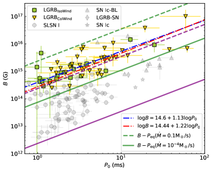
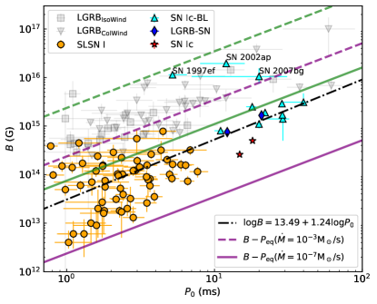
Figure 1: Left panel: $B-P_{0}$ distribution for the magnetar engines of LGRB X-ray plateaus (green squares for the isotropic wind model; yellow triangles for the collimated wind model), SLSNe I (gray circles), SNe Ic-BL without LGRBs (gray triangles), LGRB-SNe (gray diamonds) and the normal SNe Ic (gray stars). We show the fitting results for LGRB X-ray plateaus (blue dashed-dotted line for the isotropic wind model represented by Equation 1; red dashed-dotted line for the collimated wind model shown by Equation 2). The expected $B-P_{\mathrm{eq}}$ correlations (Equation A3) are displayed assuming accretion rates $\dot{M}=0.1$ (green dashed line), $10^{-3}$ (purple dashed line), $10^{-4}$ (green solid line) and $10^{-7}$ (purple solid line) M_⊙ s^-1, respectively. Right panel: We highlight the $B-P_{0}$ distribution for SLSNe I (orange circles), SNe Ic-BL without LGRBs (cyan triangles), LGRB-SNe (blue diamonds) and the normal SNe Ic (red stars). The black dashed-dotted line represents the best-fit correlation for these SNe (Equation 3). SN 1997ef, SN 2002ap and SN 2007bg are labeled due to their significant deviations from the fitting result. The LGRB X-ray plateaus are marked in gray symbols. Data references are given in Table 1.

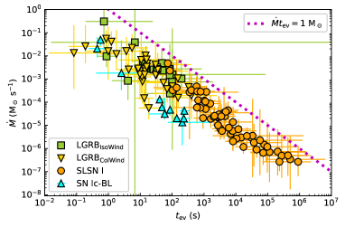
Figure 2: The accretion rate ($\dot{M}$; Equation A3) versus the lower limit of accretion timescale ($t_{\mathrm{ev}}$; Equation A4) inferred for the magnetar engines of LGRB X-ray plateaus (green squares for the isotropic wind model; yellow triangles for the collimated wind model), SLSNe I (orange circles) and SNe Ic-BL without detections of LGRBs (cyan triangles).

3.2 SLSNe I, SNe Ic and SNe Ic-BL

Core-collapse SNe usually reach their peak luminosities at tens of days after explosion. Around that time, magnetar wind should be near-isotropic and contributes most of the rotation energy to heat and/or accelerate the ejecta.

Based on the model fits to the light curves (Nicholl et al., 2017; Blanchard et al., 2018; Villar et al., 2018; Blanchard et al., 2019; Lin et al., 2020), the magnetar engines of SLSNe I are characterized by magnetic field of $10^{12}<B\lesssim 10^{14}$ G and spin with a short period of $1\lesssim P_{0}<10$ ms (Figure 1). The magnetars with longer initial spin period appear to have stronger magnetic field. This correlation possibly suggests that the engine timescale is roughly comparable to the diffusion timescale of ejecta, which corresponds to $B\propto P_{0}$ (Nicholl et al., 2017). If the physics of accretion-induced spin equilibrium could apply to the cases of SLSNe I, the inferred accretion rates based on Equation (A3) mainly fall between $10^{-7}-10^{-3}$ M_⊙ s^-1.

SNe Ic-BL might be accompanied by the birth of magnetars, since an upper limit of the kinetic energy of SNe Ic-BL (i.e. $\sim$ a few $10^{52}$ erg s^-1, model dependent though) is comparable to the maximum rotation energy of a millisecond magnetar (Mazzali et al., 2014). Moreover, some SNe Ic-BL (e.g., SN2010ay and PTF10vqv) are unlikely to be explained by radioactive ⁵⁶Ni model and hence magnetar is invoked as a dominant power source (Wang et al., 2017a). As seen from Figure 1, most SNe Ic-BL without coincident LGRBs in our sample invoke a magnetar with $P_{0}\gtrsim 10$ ms and $B\sim 10^{15}$ G, while some events require the magnetic field to be as strong as $\sim 10^{16}$ G. Associated with GRB 980425, SN 1998bw requires $B\approx 1.66\times 10^{15}$ G for the central magnetar, in agreement with most of its non-GRB peers. Compared with the SLSNe I magnetars, the magnetar candidates for SNe Ic-BL have stronger magnetic field and longer initial spin period.

Greiner et al. (2015) reported the observations of a luminous SN Ic SN 2011kl (associated with GRB 111209A), which has intermediate luminosity lying between typical SNe Ic-BL and SLSNe I. Following their fitting results, SN 2011kl could be also powered by a magnetar with an initial spin period of $P_{0}\approx 12$ ms and magnetic field of $B\approx 7.5\times 10^{14}$ G. Two normal SNe Ic (iPTF15dtg and PTF11mnb) require weaker magnetic field than most SNe Ic-BL and LGRB-SNe in our sample (Taddia et al., 2018, 2019).

We note that, although SLSNe I exhibit distinct spectral features at early times (e.g., Quimby et al., 2011, 2018), their post-peak spectra eventually evolve to resemble those of SNe Ic/Ic-BL (Pastorello et al., 2010; Liu et al., 2017; Blanchard et al., 2019; Nicholl et al., 2019). This suggests an underlying connection among these subtypes of SNe. By fitting the $B-P_{0}$ distribution of our SNe samples (including SLSNe I, SNe Ic and SNe Ic-BL), the following correlation (see also the fitting procedure described in Appendix B) is derived

$$\log B=13.49^{+0.1}_{-0.1}+(1.24^{+0.14}_{-0.14})\log P_{0},$$ (3)

which is consistent with $B-P_{\mathrm{eq}}$ correlation expected for the accreting magnetars at the spin equilibrium state. Although SNe Ic/Ic-BL require different properties of magnetars than SLSNe I, similar accretion rates are inferred for most SNe in our sample. Therefore, nascent magnetar plus the accretion disk system provide a unified picture to explain the production of SLSNe I, SNe Ic and SNe Ic-BL. Based on the magnetic propeller model, the central magnetar with low magnetic field will be accelerated to a millisecond spin period, responsible for the energy source powering an SLSN I; conversely, stronger magnetic field leads to longer equilibrium spin period of a magnetar, and it hence produces an SN Ic/Ic-BL.

Assuming that magnetars can always reach the spin equilibrium state, the lower limits for accretion timescales in the cases of SLSNe I are estimated as $t_{\mathrm{ev}}\sim 10^{2}-10^{6}$ s based on Equation (A4), while SNe Ic-BL show a similar $t_{\mathrm{ev}}$ distribution to LGRB X-ray plateaus (Figure 2). Although the limits of accretion timescales for most SLSNe I are consistent with the fallback timescale for the envelopes of the compact progenitor stars, a fraction of SLSNe I require longer accretion timescales. Assuming that the accretion timescale ($t_{\mathrm{acc}}$) is equivalent to the fallback timescale, the long-term accretion could be due to the fallback of the stellar envelope from large radii or inner ejecta that cannot escape from the central object (Chevalier, 1989; Dexter & Kasen, 2013). Since early-time bumps observed in some events could be attributed to the cooling of an shocked envelope with a radius of $\gtrsim 500R_{\odot}$ (e.g., Piro, 2015; Nicholl & Smartt, 2016; Smith et al., 2016), the immediate progenitors of a portion of SLSNe I could be surrounded by largely extended envelopes, in agreement with the first possible scenario allowing for the late accretion. Alternatively, those bumps might suggest the possible existence of circumstellar medium (CSM; Leloudas et al., 2012). In this scenario, reversed shock could be produced by the ejecta-CSM interaction. Then inner layer of the ejecta would be decelerated by the reverse shock and finally bound to the gravity of the newborn magnetar, contributing to the late accretion. It remains unknown whether SLSNe I could be associated with LGRBs. But it might be a challenge for an LGRB jet to push through the extended envelope or CSM surrounding the progenitor stars of some SLSNe I. For this subclass of SLSNe I, the magnetic field strength is found to be lower than $10^{14}$ G, which is inconsistent with the magnetic field required by LGRBs.

Figure 3 shows some examples of the spin-down luminosity (magnetic dipole radiation luminosity) evolution of isolated magnetars with $B=10^{14}-10^{16}$ G and $P=10-100$ ms. The spin-down luminosities of those magnetars usually decline below $10^{44}$ erg s^-1 after 10 days since explosion, which are insufficient to power SLSNe I according to the Arnett’s rule (the peak luminosity equals the heating luminosity at peak time). Based on the peak luminosity statistics conducted by Prentice et al. (2016), the majority of normal SNe Ic peak at a luminosity of log$(L_{\mathrm{p,Ic}})\approx 41.5-43$ and at an epoch of $10-23$ days after explosion. Since the spin-down luminosities can match the peak luminosities of normal SN Ic during their peak time, it is possible that those magnetars can produce emissions resembling the normal SNe Ic. For an accretion rate between $10^{-7}-10^{-4}$ M_⊙ s^-1, the accreting magnetars with magnetic field of $\sim 10^{14}-10^{15}$ G could reach an equilibrium spin period of $10-100$ ms, and hence possibly power normal SNe Ic. iPTF15dtg exhibits slowly declining light curves and strong Oi $\lambda$7774 emission at late phase, which can be explained in the magnetar-powered scenario (Taddia et al., 2019; Nicholl et al., 2019). However, most SNe Ic lack the engine-powered signatures, and ⁵⁶Ni decay may be the power source. SLSNe I and SNe Ic-BL are preferentially found in dwarf galaxies with low metallicity (e.g., Lunnan et al., 2014; Perley et al., 2016; Schulze et al., 2018; Modjaz et al., 2020). With such low metallicity, stellar wind from massive progenitor stars might be reduced and hence the angular momentum can be sustained to help form a rapidly rotating magnetar. As most SNe Ic prefer higher metallicity environments (e.g., Modjaz et al., 2020), it is thus expected that only a small subset of SNe Ic are accompanied by the birth of magnetars.

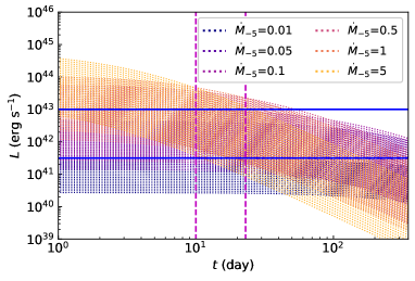
Figure 3: The spin-down luminosity evolution of magnetars with $B$ and $P_{0}$, which are adopted (1) from the parameter space limited to $B\in[10^{14},10^{16}]$ G and $P_{0}\in[10,100]$ ms, and (2) based on the $B-P$ relation for an accreting magnetar with the accretion rates $\dot{M}_{-5}=\dot{M}/(10^{-5}M_{\odot}/s)=0.01,0.05,0.1,0.5,1,5$, respectively. The blue horizon lines show the peak luminosity range of the normal SNe Ic ($41.5<\log L_{\mathrm{p,Ic}}<43$), and the purple vertical lines mark the major range of the peak time ($\approx 10-23$ days; Prentice et al., 2016).

4 Discussions and conclusions

By involving the fallback accretion effect in the magnetar-powered scenario, we tentatively shed light on the correlation between the surface magnetic field ($B$) and initial spin period ($P_{0}$) of magnetar candidates that can account for the emissions of transients, such as LGRB X-ray plateaus, SLSNe I, SNe Ic and SNe Ic-BL.

In the context of the LGRB with X-ray plateaus, it is still debated whether the magnetar wind is isotropic and collimated in the plateau phase. No matter which wind configuration, however, the initial spin periods and the surface magnetic field of the magnetars are found to follow a positive correlation in agreement with $B\propto P_{0}^{7/6}$, suggesting that fallback accretion could play a role in the spin evolution of the magnetars. Thus, the initial spin period inferred from observations could correspond to the equilibrium spin period as a result of interaction between magnetar and surrounding accretion disk. Based on the magnetic propeller model, the accretion rates of the surrounding disks are inferred to be $\dot{M}\approx 10^{-4}-10^{-1}$ M_⊙ s^-1 and the lower limits for the required accretion timescales are shorter than 1000 s, which are comparable to or shorter than the fallback timescale of the envelope of a WR star. This result is consistent with the proposal of compact progenitor stars as the progenitors of LGRBs, assuming that disk materials fall back from stellar envelope.

Magnetars are also invoked as an alternative engine to power SNe. On a timescale comparable to the rise time of core-collapse SNe, the magnetar wind should be isotropic. For SLSNe I, SNe Ic and SNe Ic-BL in our magnetar-powered sample, $B-P_{0}$ distribution is found to be also consistent with the physics of accretion-induced spin equilibrium. The inferred accretion rates can be as low as $\dot{M}\approx 10^{-7}-10^{-3}$ M_⊙ s^-1. Based on the magnetic propeller model, the central magnetars with low magnetic fields will be accelerated to a millisecond spin period, and may be able to power SLSNe I; conversely, those with stronger magnetic fields could result in longer equilibrium spin period, which could explain a portion of SNe Ic/Ic-BL.

For SLSNe I, the accretion timescales are required to be $t_{\mathrm{acc}}\gtrsim 10^{2}-10^{6}$ s. Assuming that accretion timescale is approximately equal to the fallback time, some SLSNe I of our sample could be produced in the explosions of typical WR stars, while the others that require longer-term accretion could originate from the progenitor stars surrounded by more extended envelopes or CSM, which reconciles with the implication of the early bumps observed in some events (e.g., Leloudas et al., 2012; Piro, 2015; Nicholl & Smartt, 2016; Smith et al., 2016).

Above discussions are based on a simple method, with which we estimate the constant accretion rates from $B-P_{0}$ distribution inferred from the magnetar-powered models. However, besides the early-time accretion with constant rate, the late-time decline of accretion rate can also influence the spin period of the magnetar and hence magnetar outflow can deviate from the magnetic dipole radiation luminosity evolution (e.g., Piro & Ott, 2011; Metzger et al., 2018). We expect that more observations and detailed modeling work in the future will provide further clues for the nature of these GRBs and stripped-envelope SNe.

Appendix A magnetic propeller model

The interaction between a magnetar with its surrounding disk has an effect on the spin evolution and hence the outflows of the magnetar (e.g., Piro & Ott, 2011; Gompertz et al., 2014; Gibson et al., 2017, 2018; Metzger et al., 2018). The interaction process depends on the relative locations of Alfvén radius ($r_{\mathrm{m}}$), co-rotation radius ($r_{\mathrm{c}}$) and light cylinder radius ($r_{\mathrm{L}}$). Alfvén radius is usually considered as the inner radius of the disk, where the ram pressure of the inflowing materials balances with the magnetic pressure of the magnetar. It can be given by

$$r_{\mathrm{m}}=(GM)^{-1/7}R^{12/7}B^{4/7}\dot{M}^{-2/7},$$ (A1)

where $G$ is the gravitational constant, $M$/$R$/$B$ denotes the mass/radius/magnetic field strength of the central magnetar, and $\dot{M}$ is the mass inflow rate at the inner edge of the disk. Given that inflowing materials rotate at the local Keplerian angular velocity, i.e. $\Omega_{\mathrm{K}}=(GM/r^{3})^{1/2}$, their co-rotation with the magnetar, occurs at a radius of

$$r_{\mathrm{c}}=(GM/\Omega^{2})^{1/3},$$ (A2)

where $\Omega=2\pi/P$ and $P$ are the angular velocity and spin period of the magnetar, respectively. The radius of the light cylinder is defined as $r_{\mathrm{L}}=c/\Omega$, inside which the magnetic field lines are usually considered to rotate rigidly with the magnetar.

If $r_{\mathrm{m}}<r_{\mathrm{c}}<r_{\mathrm{L}}$, materials at inner edge of the disk revolve faster than the local magnetic field lines and tend to be funneled before falling onto the surface of the magnetar. Thus, the magnetar gain its angular momentum and subsequently the co-rotation radius decreases until $r_{\mathrm{c}}\sim r_{\mathrm{m}}$. Conversely if $r_{\mathrm{c}}<r_{\mathrm{m}}<<r_{\mathrm{L}}$, the slow-rotating inner disk is speeded up to a super-Keplerian velocity by the magnetar, which results in mass ejection from disk and sharp spin-down of the magnetar (propeller regime). The spin-down of the magnetar, in return, leads to an increase of $r_{\mathrm{c}}$. Consequently, such a magnetar-disk system tends to evolve towards $r_{\mathrm{c}}=r_{\mathrm{m}}$ if the spin evolution of the magnetar is dominated by the interaction with the accretion disk. When $r_{\mathrm{c}}$ equals $r_{\mathrm{m}}$, the accreting magnetar would reach an equilibrium spin period (e.g., Piro & Ott, 2011)

$$P_{\mathrm{eq}}=2\pi(GM)^{-5/7}R^{18/7}B^{6/7}\dot{M}^{-3/7}.$$ (A3)

The equilibrium spin period is independent of the initial spin period of magnetar but correlates with the magnetic field strength and mass inflow rate. With $M=1.4$ M_⊙ and $R=12$ km, therefore, the accretion rate can be estimated from the $B-P$ distribution for accreting magnetars.

Assuming a constant accretion rate, the evolutionary timescale, before a magnetar reaches such a spin equilibrium, can be estimated by (Metzger et al., 2018)

$$t_{\mathrm{ev}}\approx\frac{2\pi I/P_{\mathrm{eq}}}{\dot{M}(GMr_{\mathrm{m}})^{1/2}}=(GM)^{2/7}IR^{-8/7}B^{-8/7}\dot{M}^{-3/7},$$ (A4)

where $I=0.35MR^{2}$ is the moment of inertia. The larger accretion rate and stronger magnetic field correspond to shorter timescale $t_{\mathrm{ev}}$. For an accreting magnetar that spins with an equilibrium period, an estimate of $t_{\mathrm{ev}}$ can be considered as the lower limit for the accretion timescale ($t_{\mathrm{acc}}$).

Appendix B Likelihood function for a linear fit

For fitting a linear function ($y=mx+c$) to data with errors on both variables, the likelihood function can be given by (D’Agostini, 2005)

$$f\propto\prod\limits_{i}\frac{1}{\sqrt{\sigma^{2}_{y_{i}}+m^{2}\sigma^{2}_{x_{i}}}}\exp\left[-\frac{(y_{i}-mx_{i}-c)^{2}}{2(\sigma^{2}_{y_{i}}+m^{2}\sigma^{2}_{x_{i}})}\right],$$ (B1)

where $x_{i}$ and $y_{i}$ are the observational quantities, and $\sigma_{x_{i}}$ and $\sigma_{y_{i}}$ are the corresponding errors.

If there exists the extra variability of data, which can be parameterized as $\sigma_{v}$, the likelihood function is modified as (D’Agostini, 2005)

$$f\propto\prod\limits_{i}\frac{1}{\sqrt{\sigma^{2}_{v}+\sigma^{2}_{y_{i}}+m^{2}\sigma^{2}_{x_{i}}}}\exp\left[-\frac{(y_{i}-mx_{i}-c)^{2}}{2(\sigma^{2}_{v}+\sigma^{2}_{y_{i}}+m^{2}\sigma^{2}_{x_{i}})}\right],$$ (B2)

By fitting the $\log B-\log P_{0}$ distribution of LGRB X-ray plateaus with Equation (B1) as the likelihood function, we obtain the correlations, i.e. Equation (1) for the isotropic wind model and Equation (2) for the collimated wind model. However, the extra variability of data ($\sigma_{v}$) should be considered for our SN sample, given the different models (see references listed in Table 1 for details) and the lack of stringent constraint on the magnetar or ⁵⁶Ni contribution. In fitting, the mean uncertainties of data is adopted as the errors for the likelihood function. For the two SNe Ic, the uncertainties of $B$ and $P_{0}$ are not given in the literature, so we set the half of the values as the corresponding uncertainties. The fitting result for the SN sample is given in Equation (3) with $\sigma_{v}=0.52^{+0.05}_{-0.04}$.

References

- Antoniadis et al. (2013) Antoniadis, J., Freire, P. C. C., Wex, N., et al. 2013, Science, 340, 448
- Blanchard et al. (2018) Blanchard, P. K., Nicholl, M., Berger, E., et al. 2018, ApJ, 865, 9
- Blanchard et al. (2019) Blanchard, P. K., Nicholl, M., Berger, E., et al. 2019, ApJ, 872, 90
- Bucciantini et al. (2009) Bucciantini, N., Quataert, E., Metzger, B. D., et al. 2009, MNRAS, 396, 2038
- Campana et al. (2006) Campana, S., Mangano, V., Blustin, A. J., et al. 2006, Nature, 442, 1008
- Chevalier (1989) Chevalier, R. A. 1989, ApJ, 346, 847
- D’Agostini (2005) D’Agostini, G. 2005, physics/0511182
- Dai & Liu (2012) Dai, Z. G., & Liu, R.-Y. 2012, ApJ, 759, 58
- Dai, & Lu (1998) Dai, Z. G., & Lu, T. 1998, A&A, 333, L87
- Dai et al. (2006) Dai, Z. G., Wang, X. Y., Wu, X. F., et al. 2006, Science, 311, 1127
- Dall’Osso et al. (2011) Dall’Osso, S., Stratta, G., Guetta, D., et al. 2011, A&A, 526, A121
- Demorest et al. (2010) Demorest, P. B., Pennucci, T., Ransom, S. M., et al. 2010, Nature, 467, 1081
- Dexter & Kasen (2013) Dexter, J., & Kasen, D. 2013, ApJ, 772, 30
- Gibson et al. (2017) Gibson, S. L., Wynn, G. A., Gompertz, B. P., et al. 2017, MNRAS, 470, 4925
- Gibson et al. (2018) Gibson, S. L., Wynn, G. A., Gompertz, B. P., et al. 2018, MNRAS, 478, 4323
- Gompertz et al. (2014) Gompertz, B. P., O’Brien, P. T., & Wynn, G. A. 2014, MNRAS, 438, 240
- Greiner et al. (2015) Greiner, J., Mazzali, P. A., Kann, D. A., et al. 2015, Nature, 523, 189
- Inserra et al. (2013) Inserra, C., Smartt, S. J., Jerkstrand, A., et al. 2013, ApJ, 770, 128
- Kasen, & Bildsten (2010) Kasen, D., & Bildsten, L. 2010, ApJ, 717, 245
- Koesterke & Hamann (1995) Koesterke, L., & Hamann, W.-R. 1995, A&A, 299, 503
- Lasky et al. (2014) Lasky, P. D., Haskell, B., Ravi, V., et al. 2014, Phys. Rev. D, 89, 047302
- Leloudas et al. (2012) Leloudas, G., Chatzopoulos, E., Dilday, B., et al. 2012, A&A, 541, A129
- Li et al. (2018) Li, L., Wu, X.-F., Lei, W.-H., et al. 2018, ApJS, 236, 26
- Lin et al. (2018) Lin, W.-L., Wang, L.-J., & Dai, Z.-G. 2018, ApJ, 855, 67
- Lin et al. (2020) Lin, W. L., Wang, X. F., Li, W. X., et al. 2020, MNRAS, 497, 318
- Liu et al. (2017) Liu, Y.-Q., Modjaz, M., & Bianco, F. B. 2017, ApJ, 845, 85
- Liu et al. (2017) Liu, L.-D., Wang, S.-Q., Wang, L.-J., et al. 2017, ApJ, 842, 26
- Lü, & Zhang (2014) Lü, H.-J., & Zhang, B. 2014, ApJ, 785, 74
- Lunnan et al. (2014) Lunnan, R., Chornock, R., Berger, E., et al. 2014, ApJ, 787, 138
- Maeda et al. (2003) Maeda, K., Mazzali, P. A., Deng, J., et al. 2003, ApJ, 593, 931
- Margalit & Metzger (2017) Margalit, B., & Metzger, B. D. 2017, ApJ, 850, L19
- Mazzali et al. (2014) Mazzali, P. A., McFadyen, A. I., Woosley, S. E., et al. 2014, MNRAS, 443, 67
- Metzger et al. (2018) Metzger, B. D., Beniamini, P., & Giannios, D. 2018, ApJ, 857, 95
- Modjaz et al. (2020) Modjaz, M., Bianco, F. B., Siwek, M., et al. 2020, ApJ, 892, 153
- Nicholl et al. (2019) Nicholl, M., Berger, E., Blanchard, P. K., et al. 2019, ApJ, 871, 102
- Nicholl et al. (2017) Nicholl, M., Guillochon, J., & Berger, E. 2017, ApJ, 850, 55
- Nicholl & Smartt (2016) Nicholl, M., & Smartt, S. J. 2016, MNRAS, 457, L79
- Pastorello et al. (2010) Pastorello, A., Smartt, S. J., Botticella, M. T., et al. 2010, ApJ, 724, L16
- Perley et al. (2016) Perley, D. A., Quimby, R. M., Yan, L., et al. 2016, ApJ, 830, 13
- Piro (2015) Piro, A. L. 2015, ApJ, 808, L51
- Piro & Ott (2011) Piro, A. L., & Ott, C. D. 2011, ApJ, 736, 108
- Prentice et al. (2016) Prentice, S. J., Mazzali, P. A., Pian, E., et al. 2016, MNRAS, 458, 2973
- Quimby et al. (2018) Quimby, R. M., De Cia, A., Gal-Yam, A., et al. 2018, ApJ, 855, 2
- Quimby et al. (2011) Quimby, R. M., Kulkarni, S. R., Kasliwal, M. M., et al. 2011, Nature, 474, 487
- Rowlinson et al. (2013) Rowlinson, A., O’Brien, P. T., Metzger, B. D., et al. 2013, MNRAS, 430, 1061
- Rowlinson et al. (2010) Rowlinson, A., O’Brien, P. T., Tanvir, N. R., et al. 2010, MNRAS, 409, 531
- Schulze et al. (2018) Schulze, S., Krühler, T., Leloudas, G., et al. 2018, MNRAS, 473, 1258
- Smith et al. (2016) Smith, M., Sullivan, M., D’Andrea, C. B., et al. 2016, ApJ, 818, L8
- Stratta et al. (2018) Stratta, G., Dainotti, M. G., Dall’Osso, S., et al. 2018, ApJ, 869, 155
- Taddia et al. (2018) Taddia, F., Sollerman, J., Fremling, C., et al. 2018, A&A, 609, A106
- Taddia et al. (2019) Taddia, F., Sollerman, J., Fremling, C., et al. 2019, A&A, 621, A64
- Usov (1992) Usov, V. V. 1992, Nature, 357, 472
- Villar et al. (2018) Villar, V. A., Nicholl, M., & Berger, E. 2018, ApJ, 869, 166
- Wang et al. (2017a) Wang, L. J., Cano, Z., Wang, S. Q., et al. 2017a, ApJ, 851, 54
- Wang et al. (2017b) Wang, L. J., Yu, H., Liu, L. D., et al. 2017b, ApJ, 837, 128
- Wang et al. (2017c) Wang, S.-Q., Cano, Z., Wang, L.-J., et al. 2017c, ApJ, 850, 148
- Woosley (2010) Woosley, S. E. 2010, ApJ, 719, L204
- Woosley & Heger (2006) Woosley, S. E., & Heger, A. 2006, ApJ, 637, 914
- Young et al. (2010) Young, D. R., Smartt, S. J., Valenti, S., et al. 2010, A&A, 512, A70
- Yu et al. (2017) Yu, Y.-W., Zhu, J.-P., Li, S.-Z., et al. 2017, ApJ, 840, 12
- Zhang et al. (2006) Zhang, B., Fan, Y. Z., Dyks, J., et al. 2006, ApJ, 642, 354
- Zhang, & Mészáros (2001) Zhang, B., & Mészáros, P. 2001, ApJ, 552, L35